





1 Introduction
From snap judgments in job interviews to the algorithmic screening of online profiles, both humans and artificial intelligence are increasingly tasked with forming consequential impressions from complex, high-dimensional data. Humans can evaluate others in as little as 100 milliseconds, with these rapid assessments predicting outcomes from hiring decisions to electoral results (Ambady & Rosenthal, Reference Ambady and Rosenthal1992; Todorov et al., Reference Todorov, Mandisodza, Goren and Hall2005). Similarly, modern AI systems now analyze vast streams of text, image, and behavioral data to make their own judgments about personality, competence, and risk. Despite this parallel function, we lack a unified theoretical and methodological framework to deconstruct and compare the judgmental processes of both human and artificial perceivers on equal terms.
The challenge of formally modeling judgment is not new. For decades, researchers have relied on Brunswik’s (Reference Brunswik1955) lens model, and its statistical formulation in Tucker’s (Reference Tucker1964) lens model equation (LME), to understand how perceivers use available cues to achieve accuracy. This framework, which underpins foundational theories like Funder’s (Reference Funder1995) Realistic Accuracy Model, has been invaluable for demonstrating how traits are perceived via relevant and detectable cues across diverse domains (Wallace & Biesanz, Reference Wallace and Biesanz2021; Rule & Ambady, Reference Rule and Ambady2008). However, the LME was conceived for a low-dimensional world, requiring researchers to hand-select a small number of potential cues. It is ill-equipped to handle the “curse of dimensionality” (Hastie et al., Reference Hastie, Tibshirani and Friedman2009) inherent in modern data, such as the thousands of dimensions generated by large language model (LLM) embeddings, which have become a cornerstone for quantifying language (Grimmer et al., Reference Grimmer, Roberts and Stewart2022).
To bridge this critical gap, we introduce the double machine learning lens model (DML-LM). By integrating the causal inference principles of double machine learning (Chernozhukov et al., Reference Chernozhukov, Chetverikov, Demirer, Duflo, Hansen, Newey and Robins2018) with the classic LME, our approach provides a robust and flexible method for analyzing how accuracy is achieved in high-dimensional settings. This innovation allows researchers to finally leverage the full richness of modern data representations, from complex text embeddings to video representations, within a structured and interpretable accuracy model.
Central to our framework is a unifying and interpretable statistic: the proportion of mediated accuracy (PoMA). PoMA provides a single, intuitive metric that quantifies the proportion of total judgmental accuracy—whether from a human or an AI—that can be statistically explained by a given set of cues. Formally, it represents the ratio of the indirect effect to the total effect (
$1 - \tau '/\tau $
 ), where
$\tau $
), where
$\tau $
 and
$\tau '$
and
$\tau '$
 denote the total and direct effects, respectively, quantifying the proportion of accuracy explained by the mediators. This allows for a principled, apples-to-apples comparison between different cue sets (e.g., traditional dictionaries vs. LLM embeddings) and different analytical models. By using PoMA, researchers can systematically evaluate how well their models capture the information used in a perceptual judgment, providing a clear path forward for dissecting the mechanisms of human intuition and algorithmic decision-making alike.
2 Theoretical and methodological framework
2.1 The lens model
By using multiple regressions to model both perceiver judgments and the validity measure (e.g., perceived intelligence and someone’s actual intelligence quotient) as a linear combination of behavioral cues, Tucker (Reference Tucker1964) quantitatively formalized Brunswik’s (Reference Brunswik1955) lens model as the LME. Specifically, by regressing our validity variable X and judgment variable Y on a vector of behavioral cues Z (where k is the number of cues), we obtain the following regression equations:

The residuals are defined as

The first parameter of interest from Tucker’s lens model, called achievement accuracy (
$r_a$
 ), is defined as the observed correlation between judgment scores and validity scores. From the above equations, the four components of the achievement correlation can be readily derived. The variance in the validity variable X and judgment variable Y can be decomposed into two components: the variance explained by the model,
$\mathrm {Var}(\hat {X})$
), is defined as the observed correlation between judgment scores and validity scores. From the above equations, the four components of the achievement correlation can be readily derived. The variance in the validity variable X and judgment variable Y can be decomposed into two components: the variance explained by the model,
$\mathrm {Var}(\hat {X})$
 , and the residual variance,
$\mathrm {Var}(e_{X})$
, and the residual variance,
$\mathrm {Var}(e_{X})$
 , which are orthogonal under ordinary least squares (OLS) regression. This yields us our traditional
$R^2$
, which are orthogonal under ordinary least squares (OLS) regression. This yields us our traditional
$R^2$
 values, interpreted as the proportion of explained variance.
$R^2$
values, interpreted as the proportion of explained variance.
$R^2$
 can also be expressed in terms of
$\text {Var}(e)$
can also be expressed in terms of
$\text {Var}(e)$
 which is mathematically equivalent to the former definition under OLS, but in general, represents how much better at the model is at predicting the outcome when compared to the average (a negative
$R^2$
which is mathematically equivalent to the former definition under OLS, but in general, represents how much better at the model is at predicting the outcome when compared to the average (a negative
$R^2$
 means the average would have been a better predictor than the model, which is possible under machine learning models but not under OLS):

$R^2_Y$
 measures the degree to which the set of cues Z are used by judges, whereas
$R^2_X$
measures the degree to which the set of cues Z are used by judges, whereas
$R^2_X$
 quantifies the degree to which the set of Z cues are related to the validity measure. The square roots of these measures (i.e., the multiple correlation R) are called the response consistency and environmental predictability coefficients, respectively (Karelaia & Hogarth, Reference Karelaia and Hogarth2008; Osterholz et al., Reference Osterholz, Breil, Nestler, Back, Letzring and Spain2021). Researchers also use these coefficients as measures of how valid the cues are and how much they are used by perceivers (Borkenau et al., Reference Borkenau, Mosch, Tandler and Wolf2016). Since these measures reflect how well the models can predict validity measure and perceiver ratings, they reflect the degree to which the entire set of cues is relevant and available (with respect to the validity measure), or detectable and utilized (with respect to the perceiver ratings; Funder, Reference Funder1995).
Two other useful statistics can be computed. The matching coefficient G (also called cue sensitivity) represents the degree of alignment between a perceiver’s usage of behavioral cues and the target itself, and is computed as the correlation between predicted values of both regression models,
$\mathrm {Cor} (\hat {X}, \hat {Y})$
 . For example, if perceivers generally use the tone of a warm voice as an indicator for agreeableness, and a warm voice tone is in fact associated with a target’s agreeableness, then G will be relatively high. The unmodeled knowledge coefficient C is computed as the correlation between the residuals of both regression models,
$\mathrm {Cor}(e_{X}, e_{Y})$
. For example, if perceivers generally use the tone of a warm voice as an indicator for agreeableness, and a warm voice tone is in fact associated with a target’s agreeableness, then G will be relatively high. The unmodeled knowledge coefficient C is computed as the correlation between the residuals of both regression models,
$\mathrm {Cor}(e_{X}, e_{Y})$
 . If perceivers had high accuracy achievement
$r_a$
. If perceivers had high accuracy achievement
$r_a$
 of strangers’ agreeableness using warm voice tone as a valid indicator, but warm voice tone wasn’t assessed and included in the regression model as a cue, then the unmodeled knowledge coefficient C might be high. Importantly, C can also indicate that cues are being used in a non-linear or non-additive manner that is not captured by the linear model.
By applying scaling terms to G and C, we can decompose total achievement
$r_a$
 into two components: modeled knowledge (
$G R_X R_Y$
into two components: modeled knowledge (
$G R_X R_Y$
 ) and unmodeled knowledge (
$C \sqrt {1-R^2_X} \sqrt {1-R^2_Y}$
) and unmodeled knowledge (
$C \sqrt {1-R^2_X} \sqrt {1-R^2_Y}$
 ). Using these scaled coefficients, we can compute the proportion of achievement that is modeled and not modeled by dividing by
$r_a$
). Using these scaled coefficients, we can compute the proportion of achievement that is modeled and not modeled by dividing by
$r_a$
 . For instance, perceivers might have an achievement of 0.5 for assessing agreeableness in strangers, where
$60\%$
. For instance, perceivers might have an achievement of 0.5 for assessing agreeableness in strangers, where
$60\%$
 (0.3) is modeled through warm voice tone, and
$40\%$
(0.3) is modeled through warm voice tone, and
$40\%$
 (0.2) is left unexplained by unknown factors (e.g., smiling and nodding). This is how Tucker (Reference Tucker1964) formally quantified Brunswik’s (Reference Brunswik1955) lens model into the LME:

This decomposition is an equality under OLS when
$k < n$
 ; under other modeling frameworks, it serves as an approximation.
2.2 Connecting the lens model and classical mediation
Although lens models are a staple for researchers conducting accuracy studies, equivalent models like the classical mediation model are used in this context as well. For instance, Stavrova and Haarmann (Reference Stavrova and Haarmann2020) fit several accuracy models using various text-based emotions via the linguistic inquiry word count (LIWC; Tausczik & Pennebaker, Reference Tausczik and Pennebaker2010) to mediate the relationship between self- and other-rated life satisfaction to identify valid and utilized textual cues. Mediation models offer a structure that is conceptually similar to the lens model, especially when considering multiple mediators. In a multiple mediator model, the relationship between an independent variable (X) and a dependent variable (Y) is transmitted through a set of k mediators (
$M_1, M_2, \ldots , M_k$
 ). The model is given by the following equations: 1) the effect of X on each mediator
$M_i$
). The model is given by the following equations: 1) the effect of X on each mediator
$M_i$
 (Path
$a_i$
(Path
$a_i$
 ):
$\hat {M}_i = a_{0,i} + a_i X \quad (\text {for } i=1, \ldots , k)$
):
$\hat {M}_i = a_{0,i} + a_i X \quad (\text {for } i=1, \ldots , k)$
 ; 2) the effect of all mediators on Y and the direct effect of X on Y (Paths
$b_i$
; 2) the effect of all mediators on Y and the direct effect of X on Y (Paths
$b_i$
 and
$\tau '$
and
$\tau '$
 ):
$\hat {Y} = b_0 + \sum _{i=1}^{k} b_i M_i + \tau 'X$
):
$\hat {Y} = b_0 + \sum _{i=1}^{k} b_i M_i + \tau 'X$
 ; and 3) the total effect of X on Y (Path
$\tau $
; and 3) the total effect of X on Y (Path
$\tau $
 ):
$\hat {Y} = \tau _0 + \tau X.$
):
$\hat {Y} = \tau _0 + \tau X.$

In a way that is analogous to the lens model’s decomposition of achievement, the mediation framework decomposes the total effect into a direct effect and the sum of all specific indirect effects. This decomposition is given by the expression:

where
$\tau $
 is the Total Effect,
$\tau '$
is the Total Effect,
$\tau '$
 is the Direct Effect, and
$\sum _{i=1}^{k} a_i b_i$
is the Direct Effect, and
$\sum _{i=1}^{k} a_i b_i$
 is the Total Indirect Effect. Thus, by fitting a mediation model using a set of cues as mediators, the classic mediation framework can also decompose accuracy (the total effect,
$\tau $
is the Total Indirect Effect. Thus, by fitting a mediation model using a set of cues as mediators, the classic mediation framework can also decompose accuracy (the total effect,
$\tau $
 ) into accuracy that is mediated through the various indirect paths (
$a_i b_i$
) into accuracy that is mediated through the various indirect paths (
$a_i b_i$
 ), or accuracy that is not captured by the mediators in linear models (the direct path,
$\tau '$
), or accuracy that is not captured by the mediators in linear models (the direct path,
$\tau '$
 ).
).
2.3 A helpful heuristic and unifying statistic: Proportion of mediated accuracy (PoMA)
To find common language between these two frameworks with disparate terminology and to lay the groundwork for incorporating double machine learning later in this article, we capitalize on this proportion of mediated accuracy concept, which we will term as
$\text {PoMA}$
 . This measure adapts the well-known proportion-mediated effect size from the mediation literature (e.g., MacKinnon, Reference MacKinnon2008; Preacher & Kelley, Reference Preacher and Kelley2011; Wen & Fan, Reference Wen and Fan2015) to the accuracy context. For the multiple mediation model, it is well known that
$\text {PoMA}_{\text {mediation}}$
. This measure adapts the well-known proportion-mediated effect size from the mediation literature (e.g., MacKinnon, Reference MacKinnon2008; Preacher & Kelley, Reference Preacher and Kelley2011; Wen & Fan, Reference Wen and Fan2015) to the accuracy context. For the multiple mediation model, it is well known that
$\text {PoMA}_{\text {mediation}}$
 can be calculated through the product-of-coefficients approach (
$\frac {\sum a_i b_i}{\tau }$
can be calculated through the product-of-coefficients approach (
$\frac {\sum a_i b_i}{\tau }$
 ) or through the difference-in-coefficients approach (
$\frac {\tau - \tau '}{\tau }$
) or through the difference-in-coefficients approach (
$\frac {\tau - \tau '}{\tau }$
 ). The former and the latter are equivalent under OLS but not under non-linear conditions like probit, logistic, or most machine learning models (MacKinnon, Reference MacKinnon2008). Since the lens model uses a standardized residual correlation (C) and regression models that yield partial coefficients with respect to other cues Z (not equivalent to mediation’s
$a_i$
). The former and the latter are equivalent under OLS but not under non-linear conditions like probit, logistic, or most machine learning models (MacKinnon, Reference MacKinnon2008). Since the lens model uses a standardized residual correlation (C) and regression models that yield partial coefficients with respect to other cues Z (not equivalent to mediation’s
$a_i$
 or
$b_i$
or
$b_i$
 ), some scaling has to be done to equate a
$\text {PoMA}_{\text {lens}}$
), some scaling has to be done to equate a
$\text {PoMA}_{\text {lens}}$
 with a
$\text {PoMA}_{\text {mediation}}$
with a
$\text {PoMA}_{\text {mediation}}$
 . The difference-in-coefficients method yields the most promising equivalenceFootnote
1
:
. The difference-in-coefficients method yields the most promising equivalenceFootnote
1
:

2.4 Challenges from high-dimensional data
While this percentage-based interpretation provides valuable insights in accuracy studies, applying these models to modern, high-dimensional data presents significant challenges. When the number of potential cues exceeds the number of observations, a common scenario with text embeddings containing hundreds or thousands of dimensions, traditional regression approaches fail. Even when the sample size is not surpassed, the assumption that high-dimensional relationships between cues, perceptions, and judgments are strictly linear and without interaction becomes untenable (for more on known limitations of mediation and equivalent models, see MacKinnon, Reference MacKinnon2008). These modeling limitations have prevented researchers from leveraging rich, high-dimensional representations of text and other complex stimuli in accuracy research.
Furthermore, using machine learning algorithms introduces a statistical complexity for the classic lens model decomposition. Unlike OLS regression, the predictions and residuals from machine learning models are not guaranteed to be independent, especially under cross-validation (Hastie et al., Reference Hastie, Tibshirani and Friedman2009). This violates a core assumption that allows for the simple decomposition of accuracy into modeled and unmodeled components seen in the classic LME. To maintain mathematical integrity, the equation must be generalized to account for these additional covariance terms, a technical expansion that is detailed in Appendix A. Figure 1 illustrates the conceptual differences between the traditional lens model and the proposed DML framework.
Comparison of the traditional lens model and the double machine learning framework.
Note: The left panel illustrates the classic Brunswik lens model, where a validity measure (X) and a judgment (Y) are modeled as linear combinations of k cues (Z). The right panel depicts the double machine learning (DML) framework, which uses machine learning models (
$m_0$
 and
$g_0$
and
$g_0$
 ) to partial out high-dimensional confounders (Z) to estimate the direct effect (
$\check {\beta }_1$
) to partial out high-dimensional confounders (Z) to estimate the direct effect (
$\check {\beta }_1$
 ) of X on Y.

Figure 1 Long description
The diagram consists of two panels.
Left Panel: Brunswik lens model.
* At the center is a vertical stack of square nodes labeled Z sub 1, Z sub 2, Z sub 3, a vertical ellipsis, and Z sub k.
* To the left is a square node X. To the right is a square node Y.
* Straight arrows point from each Z node in the center stack outward to both X and Y.
* Above the stack, a square node X-hat on the left and Y-hat on the right are connected by a curved arrow labeled G.
* Below the stack, circular nodes epsilon sub X on the left and epsilon sub Y on the right have arrows pointing up to X and Y respectively. A curved arrow labeled C connects epsilon sub X and epsilon sub Y.
Right Panel: Double machine learning D M L framework.
* The center vertical stack of Z nodes remains the same.
* To the left is square node X and to the right is square node Y.
* Instead of direct arrows from every Z node, the Z stack is grouped. An arrow labeled m sub 0 (Z) points from the Z group to X. An arrow labeled g sub 0 (Z) points from the Z group to Y.
* The top section with X-hat, Y-hat, and curved arrow G is identical to the left panel.
* In the bottom section, circular nodes epsilon sub X and epsilon sub Y have arrows pointing up to X and Y. They are connected by a straight horizontal arrow pointing from epsilon sub X to epsilon sub Y, labeled beta-check sub 1.
For our purposes, however, the primary goal remains conceptual: to partition total accuracy into the portion explained by our cues and the portion that remains unexplained. The PoMA statistic continues to serve this purpose well. Therefore, our proposed framework adopts an estimation strategy to achieve a robust estimate of this fundamental split, focusing on the unmodeled relationship after the influence of all textual cues has been partialled out.
2.5 Double machine learning
From the domain of econometrics, double machine learning has emerged as a method for partialling out high-dimensional confounding variables (a large numbers of potential confounders, possibly exceeding the sample size) to enable unbiased estimation of regression coefficients (Chernozhukov et al., Reference Chernozhukov, Chetverikov, Demirer, Duflo, Hansen, Newey and Robins2018). Chernozhukov demonstrated that using non-parametric machine learning algorithms
$m_0$
 and
$g_0$
and
$g_0$
 (e.g., random forests, neural networks, etc.) to directly partial out high-dimensional confounding variables Z on an independent variable X and dependent variable Y can result in a biased estimate of the slope parameter
$\beta _1$
(e.g., random forests, neural networks, etc.) to directly partial out high-dimensional confounding variables Z on an independent variable X and dependent variable Y can result in a biased estimate of the slope parameter
$\beta _1$
 (denoted as
$\theta $
(denoted as
$\theta $
 in their paper).
Chernozhukov et al. (Reference Chernozhukov, Chetverikov, Demirer, Duflo, Hansen, Newey and Robins2018) optimize for an alternative score function while using a technique called Neyman orthogonalization to prevent regularization biases from biasing the estimation of
$\beta _1$
 , where
$e_{X} = X - \hat {m}_0(Z)$
, where
$e_{X} = X - \hat {m}_0(Z)$
 (
$\hat {m}_{0}$
(
$\hat {m}_{0}$
 estimated using an auxiliary sample
$I^{c}$
estimated using an auxiliary sample
$I^{c}$
 ). By implementing Neyman orthogonalization alongside a cross-fitting procedure (sample-splitting and then swapping the roles of main and auxiliary samples to produce multiple estimates for averaging into a final statistic
$\check {\beta }_{1}$
). By implementing Neyman orthogonalization alongside a cross-fitting procedure (sample-splitting and then swapping the roles of main and auxiliary samples to produce multiple estimates for averaging into a final statistic
$\check {\beta }_{1}$
 ), they found that
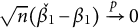
$\sqrt {n}(\check {\beta _{1}} - \beta _{1}) \xrightarrow {p} 0$
), they found that
$\sqrt {n}(\check {\beta _{1}} - \beta _{1}) \xrightarrow {p} 0$
 . In sum, removal of regularization biases through orthogonalization and cross-fitting made
$\beta _1$
. In sum, removal of regularization biases through orthogonalization and cross-fitting made
$\beta _1$
 estimation robust to errors in estimating
$m_0$
estimation robust to errors in estimating
$m_0$
 and
$g_0$
and
$g_0$
 , producing an unbiased and consistent estimator
$\check {\beta }_{1}$
, producing an unbiased and consistent estimator
$\check {\beta }_{1}$
 for regressing Y on X while addressing high-dimensional confounders (denoted as
$\check \theta $
for regressing Y on X while addressing high-dimensional confounders (denoted as
$\check \theta $
 in their paper). Theorems 3.1 and 3.2 in Chernozhukov’s paper outline the point estimate and asymptotic variance of
$\check {\beta }_1$
in their paper). Theorems 3.1 and 3.2 in Chernozhukov’s paper outline the point estimate and asymptotic variance of
$\check {\beta }_1$
 , translated using our notation below:


2.5.1 Connecting DML to the mediation and lens model
Although mediation and lens models are not necessarily concerned about confounders, DML does share many similarities with the lens model in terms of structure. Both frameworks use a set of variables Z to predict X and Y variables. Both yield a direct effect akin to a regression coefficient (Chernozhukov’s
$\check {\beta _{1}}$
 and the lens model’s
$C \sqrt {\frac {1-R^2_{Y}}{1-R^2_{X}}}$
and the lens model’s
$C \sqrt {\frac {1-R^2_{Y}}{1-R^2_{X}}}$
 , comparable to the mediation framework’s
$\tau '$
, comparable to the mediation framework’s
$\tau '$
 ).
).
We can apply the difference-in-coefficients approach to get an estimate of
$\text {PoMA}$
 for the double machine learning approach, and although these estimates will not yield the same values as the product-of-coefficients approach under non-linear models, this coefficient can be easily interpreted as the reduction in total effect after using cross-fitted machine learning methods to control for a set of high-dimensional confounders. Thus,
$\text {PoMA}_{\text {DML}}$
for the double machine learning approach, and although these estimates will not yield the same values as the product-of-coefficients approach under non-linear models, this coefficient can be easily interpreted as the reduction in total effect after using cross-fitted machine learning methods to control for a set of high-dimensional confounders. Thus,
$\text {PoMA}_{\text {DML}}$
 would be interpreted as the proportion of accuracy reduced by controlling cues with machine learning. In the causal mediation framework, this is a function of what is referred to as the controlled direct effect (not to be confused with the natural direct effect; Imai et al., Reference Imai, Keele and Tingley2010). By establishing a baseline total effect of
$\beta _{1}$
would be interpreted as the proportion of accuracy reduced by controlling cues with machine learning. In the causal mediation framework, this is a function of what is referred to as the controlled direct effect (not to be confused with the natural direct effect; Imai et al., Reference Imai, Keele and Tingley2010). By establishing a baseline total effect of
$\beta _{1}$
 (a simple regression coefficient from regressing Y on X that is the same as
$\tau $
(a simple regression coefficient from regressing Y on X that is the same as
$\tau $
 in mediation), we can express this proportion with the following equation:

Despite nuanced differences between causal and classical mediation frameworks, modern high-dimensional mediation researchers still use measures analogous to
$\text {PoMA}$
 for their ease of use and interpretability, like Chang et al.’s Global Mediation Percentage (Reference Chang, Fang, Gorczyca, Batmanghelich and Tseng2025). Because these are ratio measures, researchers should ensure they have sufficient sample size and an effect size that does not hover too close to zero to avoid estimate instability (MacKinnon, Reference MacKinnon2008).
Finally, it is important to emphasize where the Brunswikian lens model and double machine learning overlap and where they diverge. They are similar in that both implement orthogonalization (i.e., creating residuals by regressing X and Y on Z). However, the lens model does not incorporate cross-fitting. Rather, the regression models make predictions and residuals on the same sample observations on which they were trained. For flexible machine learning methods that can memorize the training data, this can result in prediction accuracy that looks artificially high due to overfitting, residuals with much less variance, and an artificially high
$\text {PoMA}$
 that is not robust. By implementing Chernozhukov et al.’s cross-fitting, we can obtain lens model statistics (including
$R^2$
that is not robust. By implementing Chernozhukov et al.’s cross-fitting, we can obtain lens model statistics (including
$R^2$
 , C, and
$\text {PoMA}$
, C, and
$\text {PoMA}$
 ) that are more valid, less biased, and more generalizable.
3 The present study
To evaluate the use of flexible machine learning methods within the lens model framework, the present study introduces the DML-LM, a method for deconstructing judgment processes in flexible and high-dimensional settings, enabling the investigation of both human and artificial perceivers of complex data types with potentially non-linear and interactive relationships. We note that while we use anthropomorphic terms like “perception,” “judgment,” and “assessment” to describe AI outputs to maintain conceptual consistency with the lens model literature, these terms refer strictly to the model’s statistical classifications and do not imply conscious awareness. The DML-LM introduced here is modality-agnostic, making it ideal for building.
Our primary aims are designed to first establish the performance of various text representations, learning algorithms, and dimensionality reduction techniques, and then to apply a balanced approach (in terms of parsimony and predictiveness) to a rich, real-world dataset. This involves three key steps:
1. Which text representation is most effective? First, we must first identify the highest-quality inputs. To do this, we leverage our largest available dataset (
$n = 9,513$
 ) to compare the efficacy of different text representation methods, from traditional LIWC dictionaries to modern language model embeddings (all-MiniLM-L6-v2 and NV-Embed-v2). This comparison, focused on the AI Accuracy model, allows us to determine which method best captures the cues relevant to perceptual accuracy.
2. What is the optimal analytical pipeline? We then conduct a comparison of 45 analytical models, systematically contrasting various machine learning algorithms (OLS, Ridge, Lasso, XGBoost, and Random Forest) and dimensionality levels. This allows us to identify the most effective and robust combination of techniques for predicting outcomes and maximizing the explained accuracy (
$\text {PoMA}$
 ) within the DML-LM.
3. How do we apply the DML-LM to deconstruct judgment? With an optimal pipeline established, we apply the full framework twice to analyze 9,513 aspirational essays written by 11-year-olds in 1969. We conduct the core analyses of AI Accuracy (on the full dataset), human accuracy (on a subset with complete human ratings,
$n = 547$
 ), and their consensus to deconstruct how humans and AI perceives social class from text. This serves as a powerful case study for uncovering the specific linguistic mechanisms that drive algorithmic bias and the “kernel-of-truth” phenomenon.
By achieving these aims, we demonstrate the utility of the DML-LM as a comprehensive and flexible toolkit for dissecting the perceptual models of both human and artificial agents. This research paves the way for a new generation of studies into person perception, stereotypes, and algorithmic fairness that are more accurate and transparent.
3.1 Methods
3.1.1 Data source
This study utilizes data from the National Child Development Study (NCDS), a highly influential and ongoing longitudinal cohort study that has followed the lives of all individuals born in a single week of March 1958 across England, Scotland, and Wales. The richness and breadth of the NCDS make it an unparalleled resource for life-course research. For the present study, we analyzed 9,513 aspirational essays collected in 1969 when the cohort members were 11 years old. Participants were given the prompt: “Imagine you are now 25 years old. Write about the life you are leading, your interests, your home life, and your work.” The resulting essays averaged 197.7 words in length (
$SD = 105.6$
 ). These texts provide a unique window into the hopes and societal understandings of children from that era. Crucially, extensive demographic information, including the social class validity used in this study, was collected concurrently through home interviews with parents and standardized assessments with the children, providing a rich context for the essay data. All study procedures were approved by the University of British Columbia’s Behavioral Research Ethics Board (BREB No. H20-01189).
3.2 Measures
3.2.1 Social class validity
The ground-truth measure of each child’s social class was based on the Registrar General’s Social Classes (RGSC) classification of their father’s occupation, as recorded in 1969. The RGSC was the United Kingdom’s official social classification system for much of the 20th century and provides a reliable indicator of socioeconomic standing for the period. This five-point ordinal scale ranks occupations by their perceived standing in the community: Class I (professional occupations, e.g., doctor and lawyer), Class II (managerial/technical, e.g., teacher and manager), Class III (skilled, both manual and non-manual, e.g., carpenter and clerk), Class IV (partially skilled, e.g., farm worker and bus conductor), and Class V (unskilled, e.g., laborer and cleaner). For our analyses, these classes were reverse-coded (1–5) so that higher values indicate higher social class
$(M = 2.92, SD = 0.89)$
 .
.
3.2.2 Social class judgment
To generate a set of perceptual judgments, we used a leading quantized, open-source LLM (AWQ Qwen 2.5 32B; Qwen et al., Reference Qwen, Yang, Zhang, Hui, Zheng, Yu, Li, Liu, Huang, Wei, Lin, Yang, Tu, Zhang, Yang, Yang, Zhou, Lin, Dang and Qiu2024) to rate each of the 9,513 essays. The use of a quantized model allows for efficient processing on local hardware of the large dataset without a prohibitive loss in performance (Lin et al., Reference Lin, Tang, Tang, Yang, Chen, Wang, Xiao, Dang, Gan and Han2024). The AI was prompted with an adapted version of the well-validated MacArthur Scale of Subjective Social Status (see Appendix B). This prompt frames the task in intuitive terms, asking the AI to place the essay writer’s family on a 10-point ladder representing their standing in society, from the “worst off” at the bottom to the “best off” at the top. The resulting AI ratings demonstrated substantial consistency with averaged ratings from 10 human raters (randomly selected from an overall pool of 600 human raters) who performed the same task
$(r(545) = 0.65)$
 , suggesting the AI’s perceptual model shares significant variance with human social perception. The achievement accuracy, or the zero-order correlation between the AI’s judgments and the actual social class validity, was modest but significant
$(r(9511) = 0.24, \ p<0.001)$
, suggesting the AI’s perceptual model shares significant variance with human social perception. The achievement accuracy, or the zero-order correlation between the AI’s judgments and the actual social class validity, was modest but significant
$(r(9511) = 0.24, \ p<0.001)$
 , indicating the AI was capturing some signal of social class from the text, and to a similar magnitude as human perceivers (
$r(545) = 0.26, \ p < 0.001$
, indicating the AI was capturing some signal of social class from the text, and to a similar magnitude as human perceivers (
$r(545) = 0.26, \ p < 0.001$
 ). See Appendix C for details on our 600 human perceivers and Appendix D for the distributions of social class judgments and the validity measure. In our application, the validity measure X is actual social class, and we examine two sets of judgments Y: AI perception and human perception.
3.3 Text representation methods
To quantify the textual cues within the essays that could potentially mediate the AI’s accuracy (these represent different methods to identify and assess the set of Z cue variables), we compared three distinct and representative methods, spanning from traditional to state-of-the-art.
3.3.1 Linguistic inquiry and word count
Representing a classic, theory-driven approach, we used the LIWC-22 software to analyze the essays. This method works by counting the percentage of words in a text that fall into 118 predefined psychological and linguistic categories (e.g., analytic, affect, and power; Boyd et al., Reference Boyd, Ashokkumar, Seraj and Pennebaker2022). The strength of LIWC lies in its interpretability, but its reliance on fixed dictionaries means it cannot capture semantic meaning, context, or novel language use. A small percentage (0.07%) of data points were invalid or missing upon exiting LIWC-22, primarily involving the Tone variable. We used scikit-learn’s Iterative Imputer to resolve these data points to refrain from using listwise deletion.
3.3.2 All-MiniLM-L6-v2 embeddings
Using knowledge distillation (training a language model by having it learn from the self-attention module of a larger language model), Wang et al. (Reference Wang, Bao, Huang, Dong and Wei2021) created the popular sentence-transformer model, MiniLMv2—capable of retaining comparable performance to the teacher model, BERT-base. We used a six-layer version of this lightweight embedding model to generate a 384-dimensional vector embedding for each essay. Consisting of only 22.7M parameters, this model is capable of running on most modern machines locally, while still capturing the semantic meaning of the entire essay in a dense numerical vector. This model is optimized for speed, making it a practical choice for many applications, and provides a strong baseline for the performance of compact language models.
3.3.3 NV-Embed-v2 embeddings
To assess the capabilities of a larger, state-of-the-art model, we also generated 4,096-dimensional vector embeddings for each essay using NV-Embed-v2, a 7.85B parameter embedding model (Lee et al., Reference Lee, Roy, Xu, Raiman, Shoeybi, Catanzaro and Ping2025). The larger parameter count, along with a novel latent attention mechanism for better pooled embedding output provide the theoretical capacity to capture more subtle and complex nuances of language, potentially leading to higher predictive accuracy at the cost of increased computational resources.
By including these three methods, our analysis is designed to span the full spectrum of text representation, from classic, interpretable dictionaries to efficient, modern embeddings and large-scale, high-performance models.
4 Data analytic plan
Our analytical approach sought to systematically uncover a model that balances parsimony and predictive power. This involved three major phases: first, establishing an optimal methodological pipeline; second, applying the full DML-LM framework to the data; and third, performing supplementary and interpretive analyses to validate and understand the results.
4.1 Phase 1: Establishing the optimal analytical pipeline
It was necessary to identify the most effective combination of text representations and learning algorithms given the many permutations. To do this, we conducted a comparison of 45 models crossing three text feature sets, five learning algorithms, and three dimensionalities. This comparison leveraged our largest available dataset (
$n = 9,513$
 ) consisting of AI Accuracy data, with performance robustly estimated using a five-fold cross-validation procedure for all models to ensure generalizability. Our three distinct text representation methods (LIWC dictionaries, all-MiniLM-L6-v2 embeddings, and NV-Embed-v2 embeddings) were evaluated under five learning algorithms (OLS, Ridge Regression, Lasso Regression, XGBoost, and Random Forest) chosen to span a spectrum of complexity and assumptions. These were applied to the data at three levels of dimensionality (Full dimensionality, 200 principal components, and the top six most predictive principal components; see Figure 2 for a conceptual visualization) to examine how model performance is retained as models move toward parsimony.
Conceptual illustration of dimensionality reduction techniques for the DML-LM.
Note: A conceptual illustration of how different approaches handle the high-dimensional cues (Z). Panel (a) represents the full, unstructured feature set. Panel (b) illustrates a dimensionality reduction (e.g., principal component analysis), where the original features are combined into a smaller set of broader components. Panel (c) depicts a feature selection approach (e.g., Lasso) which identifies and retains a sparse subset of the most important original features.

Figure 2 Long description
The diagram consists of three vertically stacked panels labeled a, b, and c. Each panel shares a common structural layout with a central vertical rectangle containing a set of cues Z, flanked by variables X on the left and Y on the right.
* Panel a shows the central rectangle filled with a dense, unstructured cloud of small dots of varying grayscale intensities. Arrows point from the rectangle to m sub 0 hat (Z) on the left and g sub 0 hat (Z) on the right, which then point to X and Y respectively. At the bottom, epsilon sub X and epsilon sub Y are connected by a horizontal arrow labeled beta sub 1 check.
* Panel b maintains the same external structure but overlays the central cloud of dots with several large, thick black circles. These circles encompass groups of the original dots, representing the aggregation of features into broader components.
* Panel c maintains the same external structure but modifies the central rectangle. Most of the original dots and several circles are now rendered in light gray dashed lines. Only a small, sparse subset of four thick black circles remains highlighted, representing the selection of specific important features.
4.1.1 Learning algorithms
The predictive performance of several statistical learning algorithms was evaluated. These models were chosen to span a range of functional forms and complexities, from a simple linear baseline to powerful, non-linear ensemble methods.
Ordinary least squares: OLS was included as a simple, interpretable baseline. It identifies the optimal linear model by minimizing the sum of the squared differences between observed and predicted outcomes (i.e., the sum of squared residuals). While its coefficients are easily interpretable, the reliability of OLS depends on strict statistical assumptions, including linearity in parameters, independence of errors, and homoscedasticity (Greene, Reference Greene2003). In high-dimensional settings, where the number of features is large relative to the number of observations, OLS models are highly susceptible to overfitting and exhibit high variance, providing a crucial benchmark against which the performance gains from more complex models can be measured (Hastie et al., Reference Hastie, Tibshirani and Friedman2009).
Ridge and lasso regression: To directly address the challenges of high-dimensionality within a linear framework, two regularized regression models were included. Both methods augment the OLS loss function with a penalty term to constrain the size of the coefficients, thereby reducing model variance. To ensure an optimal level of regularization was applied, we used cross-validating versions of each model. Ridge regression, which uses an
$L_2$
 penalty (
$\lambda \sum _{j=1}^{p} \beta _j^2$
penalty (
$\lambda \sum _{j=1}^{p} \beta _j^2$
 ) to handle multicollinearity (Hoerl & Kennard, Reference Hoerl and Kennard1970), was implemented with RidgeCV, which uses efficient leave-one-out cross-validation to select the best regularization strength. In contrast, Lasso regression, which uses an
$L_1$
) to handle multicollinearity (Hoerl & Kennard, Reference Hoerl and Kennard1970), was implemented with RidgeCV, which uses efficient leave-one-out cross-validation to select the best regularization strength. In contrast, Lasso regression, which uses an
$L_1$
 penalty (
$\lambda \sum _{j=1}^{p} |\beta _j|$
penalty (
$\lambda \sum _{j=1}^{p} |\beta _j|$
 ) to perform automatic feature selection (Tibshirani, Reference Tibshirani1996), was tuned via an internal five-fold cross-validation through LassoCV. Although ridge and lasso regression are capable of using interaction terms, no interaction terms were included due to the lack of apriori theory behind why certain embeddings or feature sets would interact with each other, and the overwhelming number of potential combinations for all possible interactions. For automatic detection of complex interactions and greater flexibility beyond linear models, we turn to machine learning methods like extreme gradient boosting (XGBoost) and random forests, detailed below.
XGBoost: As a powerful, non-linear model, XGBoost was included. XGBoost is a highly efficient implementation of the gradient boosting framework that sequentially builds decision trees to correct prior errors (Chen & Guestrin, Reference Chen and Guestrin2016). To provide a fair, out-of-the-box baseline, the model was run with the default hyperparameters from the xgboost library without specific tuning, allowing for a direct comparison against other standard models without extensive, model-specific optimization. For computational efficiency, the GPU tree construction method was used.
Random forest: A second non-linear ensemble method, Random Forest, was also included. A Random Forest operates by constructing a multitude of decision trees at training time and outputting their mean prediction (Breiman, Reference Breiman2001). We utilized an implementation with 100 trees and allowed trees to grow to their maximum depth. While many studies employ larger ensembles (e.g., 500 or 1,000 trees; Belgiu & Drăguţ, Reference Belgiu and Drăguţ2016; Probst et al., Reference Probst, Wright and Boulesteix2019), methodological research indicates that the vast majority of predictive gains are realized within the first 100 trees (Oshiro et al., Reference Oshiro, Perez and Baranauskas2012). Robustness checks conducted with 1,000 trees confirmed that increasing the ensemble size yielded consistent substantive conclusions. While we observed variation in judgmental matching, which increased from 0.65 to 0.74 as predictions stabilized to parity with linear benchmarks (e.g., Lasso on 200 PCs yielded
$G \approx 0.74$
 ), this improvement does not alter the study’s core findings. Given our specific focus on decomposing accuracy to determine the extent to which cues capture judgment, the primary estimands of interest are the unmodeled direct effect, the unmodeled knowledge, and the resulting PoMA. These critical parameters remained robust to hyperparameter tuning. Specifically,
$\check {\beta }$
), this improvement does not alter the study’s core findings. Given our specific focus on decomposing accuracy to determine the extent to which cues capture judgment, the primary estimands of interest are the unmodeled direct effect, the unmodeled knowledge, and the resulting PoMA. These critical parameters remained robust to hyperparameter tuning. Specifically,
$\check {\beta }$
 remained virtually identical across conditions (
$\Delta < 0.001$
remained virtually identical across conditions (
$\Delta < 0.001$
 ), resulting in a negligible shift in the final PoMA metric (change of
$< 0.001$
), resulting in a negligible shift in the final PoMA metric (change of
$< 0.001$
 , e.g., 0.599 vs. 0.598). Because the 1,000-tree specification required a 20-fold increase in computational cost without changing the estimate of cue-based accuracy, we retained the 100-tree specification for the final analysis to prioritize reproducibility and efficiency.
4.1.2 Feature sets of decreasing dimensionality
To assess model performance under varying levels of complexity, three distinct feature sets were created. The first utilized the full dimensionality of the feature sets to establish a performance baseline. The second employed principal component analysis (PCA) to create a reduced feature set, retaining 200 components for the embedding methods and 30 for LIWC. While other dimensionality reduction techniques exist, PCA was selected due to its ubiquity across computer science, statistics, and psychology, as well as its specific efficacy with LLM embeddings. Recent work indicates that embeddings reduced by 50% via PCA retain over 90% of their predictive performance (Takeshita et al., Reference Takeshita, Takeshita, Ruffinelli and Ponzetto2025). Indeed, LLM embeddings exhibit substantial redundancy; removing even 90% of dimensions often results in less than 10% performance degradation (Kataiwa et al., Reference Kataiwa, Hakaze and Ohki2025; Takeshita et al., Reference Takeshita, Takeshita, Ruffinelli and Ponzetto2025; Tsukagoshi & Sasano Reference Tsukagoshi and Sasano2025). Furthermore, psychological research suggests that despite their high dimensionality, the semantic structure of LLM embeddings can effectively be mapped onto the same low-dimensional subspace as human semantics—specifically the three dimensions of evaluation, potency, and activity described by Osgood et al.’s (Reference Osgood, Suci and Tannenbaum1957) Semantic Differential (Kozlowski et al., Reference Kozlowski, Dai and Boutyline2025). Taken together, PCA represents an effective strategy for isolating the core semantic dimensions that mediate the relationship between social class and judgment while systematically pruning redundant dimensions.
To ensure features with larger scales did not disproportionately influence the analysis, particularly regarding the coefficient shrinkage in lasso and ridge regression, all data were standardized before and after the PCA transformation. This number of components was chosen as a way to reduce the subspace to a reasonable dimensionality and level of explained variance (94.7% for MiniLM, 73.7% for NV-Embed, and 61.7% for LIWC). Critically, while the DML framework is capable of handling highly complex non-linear associations, we utilized PCA, a linear reduction technique, to preserve the option for interpretability. Note that while PCA itself is a linear transformation, the resulting components can still be used as inputs to non-linear modeling approaches such as XGBoost, preserving the capacity to capture non-linear relationships in subsequent modeling stages. This choice serves a diagnostic function: by comparing the performance of these linear features against flexible non-linear estimators, we can empirically determine if substantial predictive power is lost to linearity. The negligible performance gap observed in this study validates that these interpretable linear components effectively capture the signal without sacrificing the explanatory power of more complex models. Finally, a highly parsimonious set with only six components was created to test model performance under conditions of extreme simplicity, a choice justified by its analogy to traditional psychological studies that rely on a small handful of core predictors (Cooksey, Reference Cooksey1996).
4.1.3 Performance evaluation
Performance was systematically evaluated using metrics central to the DML-LM, including judgmental consistency (
$R^2_Y$
 ), environmental predictability (
$R^2_X$
), environmental predictability (
$R^2_X$
 ), and
$\text {PoMA}$
), and
$\text {PoMA}$
 . For robustness and comparability with the classic literature, these were supplemented with traditional lens model statistics, such as the matching coefficient and the residual correlation. To ensure our estimates are generalizable and not susceptible to overfitting, all models were evaluated using a five-fold cross-validation procedure. We report the mean cross-validated
$R^2$
. For robustness and comparability with the classic literature, these were supplemented with traditional lens model statistics, such as the matching coefficient and the residual correlation. To ensure our estimates are generalizable and not susceptible to overfitting, all models were evaluated using a five-fold cross-validation procedure. We report the mean cross-validated
$R^2$
 across all folds, supplemented by the simple value-prediction correlation (e.g.,
$\text {Corr}(X, \hat {X})$
across all folds, supplemented by the simple value-prediction correlation (e.g.,
$\text {Corr}(X, \hat {X})$
 ), which offers a more stable and intuitive measure of predictive accuracy, particularly in settings where
$R^2$
), which offers a more stable and intuitive measure of predictive accuracy, particularly in settings where
$R^2$
 values can be negative (Hastie et al., Reference Hastie, Tibshirani and Friedman2009).
4.2 Phase 2: Applying the DML-LM to decompose human–AI accuracy
Upon establishing a model pipeline that balanced parsimony, computational efficiency, and predictive power, we applied the DML-LM across three analyses. First, we used the DML-LM to fit an AI-accuracy model utilizing the full dataset (
$n=9,513$
 ), regressing AI ratings on the validity measure. Second, we fit a human-accuracy model utilizing the subset of data with complete human ratings (
$n=547$
), regressing AI ratings on the validity measure. Second, we fit a human-accuracy model utilizing the subset of data with complete human ratings (
$n=547$
 ), regressing human ratings on the validity measure. Finally, we applied the DML-LM to fit a human–AI consensus model by regressing AI ratings on human ratings, an approach analogous to studies that reconcile data from different sources like parents and teachers (Fleece & Teglasi, Reference Fleece and Teglasi2024). This allowed us to understand the model’s shared cue utilization and the extent to which unmeasured cues were shared between human and AI ratings. The same performance metrics from first analytic phase are reported across all three applications of the DML-LM.
4.3 Phase 3: Interpretive analysis of core cues
To move from prediction to explanation, we conducted a two-part interpretive analysis involving post-lasso coefficients and topic modeling to understand the magnitude of cue utilization and validity, as well as the substance of specific principal components.
4.3.1 Post-lasso coefficients
First, to obtain non-shrunken estimates of the specific weight of each principal component in our final model, we employed a post-Lasso OLS approach. While the main Lasso procedure is ideal for feature selection and building robust predictive models, its coefficients are intentionally shrunk toward zero and are thus biased, a property that improves out-of-sample prediction but makes the coefficients themselves unsuitable for direct inferential interpretation (Tibshirani, Reference Tibshirani1996). To generate estimates suitable for inference, the post-selection OLS method refits a standard OLS model using only the subset of features that were selected by the Lasso algorithm. This technique yields asymptotically unbiased coefficients and permits valid statistical inference for the selected predictors, overcoming the challenges posed by Lasso’s original, shrunken estimates (Belloni & Chernozhukov, Reference Belloni and Chernozhukov2013; Hastie et al., Reference Hastie, Tibshirani and Friedman2009). The validity of this naïve post-selection approach is further supported by recent work, where Zhao et al. (Reference Zhao, Witten and Shojaie2021) established that with sufficiently large samples, the variable set selected by the lasso can be considered deterministic with high probability. This finding provides an asymptotic justification for applying standard inferential tools directly to the post-selection OLS model to achieve valid inference.
4.3.2 BERTopic model for topic-variable associations
To translate the opaque principal components into interpretable constructs, we first selected the 15 most impactful components for analysis. This selection was based on the magnitude of their post-Lasso OLS feature weights in a model predicting a composite of the validity measure, AI ratings, and human ratings. Next, using a methodology inspired by BERTopic (Grootendorst, Reference Grootendorst2022), we generated topic-based descriptions for the positive and negative poles of these 15 components. We began by using UMAP to reduce the essay embeddings to three dimensions, which we then clustered into hundreds of high-resolution topics with HDBSCAN. For each topic cluster, we extracted representative keywords using a class-based TF-IDF algorithm and calculated the cluster’s mean score on our main variables (the 15 PCs, validity, and AI/human judgments). A topic was defined as “high” or “low” on a variable if its mean score fell in the top or bottom quartile of all topic means, respectively. Finally, to visualize these relationships, we plotted the topic clusters in the 3D UMAP space and drew lines connecting the highest- and lowest-scoring cluster for each PC. To clarify the thematic content of each PC’s poles, we also generated word clouds based on the vocabulary of its six most extreme topic clusters (the top three and bottom three).
5 Results
5.1 The macro view: Which models performed best?
5.1.1 Language model embeddings surpass dictionary methods
A clear performance hierarchy emerged among the text representation methods. State-of-the-art language model embeddings significantly outperformed the traditional LIWC dictionary-based approach across all key metrics. The optimal model, combining the NV-Embed feature set with OLS, Lasso, or Ridge regression and 200 principal components, achieved the highest cross-validated environmental predictability (
$R^2_{X}= 0.11$
 ) and judgmental consistency (
$R^2_{Y_{AI}}=0.56$
) and judgmental consistency (
$R^2_{Y_{AI}}=0.56$
 ). The Lasso model using MiniLM embeddings also proved highly effective, performing about four-fifths of the NV-Embed embedding performance (
$R^2_{X} = 0.09$
). The Lasso model using MiniLM embeddings also proved highly effective, performing about four-fifths of the NV-Embed embedding performance (
$R^2_{X} = 0.09$
 ,
$R^2_{Y_{AI}}=0.44$
,
$R^2_{Y_{AI}}=0.44$
 ), with OLS and Ridge offering near identical performance. Both NV-Embed and Mini-LM embedding methods substantially exceeded the performance of the best LIWC-based model (
$R^2_{X}$
), with OLS and Ridge offering near identical performance. Both NV-Embed and Mini-LM embedding methods substantially exceeded the performance of the best LIWC-based model (
$R^2_{X}$
 = 0.06,
$R^2_{Y_{AI}}$
= 0.06,
$R^2_{Y_{AI}}$
 = 0.34; see Figure 3). See Table 1 for the complete set of results.
Model performance in predicting AI judgments and the social class validity.
Note: The scatterplots compare the cross-validated (CV) judgmental consistency (
$R^2_{Y_{AI}}$
 ) against the environmental predictability (
$R^2_X$
) against the environmental predictability (
$R^2_X$
 ) for five learning algorithms (OLS, XGBoost, Lasso, Ridge, and Random Forest [RF]) across three text representation methods (LIWC, MiniLM, and NV-Embed). Marker color corresponds to the dimensionality of the feature sets used, where black is the full dimensionality, dark gray is the complete set of 200 PCs (or 30, in the case of LIWC), and light gray is the set of top 6 PCs. Two data points representing models with full NV-Embed features were omitted to improve axis scaling: OLS (
$R^2_{X} = -0.94$
) for five learning algorithms (OLS, XGBoost, Lasso, Ridge, and Random Forest [RF]) across three text representation methods (LIWC, MiniLM, and NV-Embed). Marker color corresponds to the dimensionality of the feature sets used, where black is the full dimensionality, dark gray is the complete set of 200 PCs (or 30, in the case of LIWC), and light gray is the set of top 6 PCs. Two data points representing models with full NV-Embed features were omitted to improve axis scaling: OLS (
$R^2_{X} = -0.94$
 ) and Ridge (
$R^2_{X} = -0.68$
) and Ridge (
$R^2_{X} = -0.68$
 ).
).

Figure 3 Long description
A three-panel scatterplot series. All panels share a common Y-axis labeled R super 2 sub Y sub A I (C V) ranging from 0.1 to 0.7, and an X-axis labeled R super 2 sub X (C V) ranging from -0.1 to 0.1.
* Legend: Five algorithms are represented by shapes: O L S (circle), X G Boost (square), Lasso (star), Ridge (diamond), and R F (triangle). Feature dimensionality is indicated by color: black (Full), dark gray (P C A), and light gray (Few).
* L I W C Panel: Data points are clustered in the lower-left and center. Squares (X G Boost) are positioned on the left near X equals -0.1. A cluster of triangles, stars, and diamonds appears on the right between X equals 0 and 0.1, with Y-values between 0.2 and 0.4.
* Mini L M Panel: Shows a tighter upward trend. Black and dark gray markers for O L S, Lasso, and Ridge are concentrated in the top-right quadrant near X equals 0.1 and Y equals 0.4. Light gray markers (Few features) are lower and further left.
* N V-Embed Panel: Displays the highest performance. Data points extend further toward the top-right corner. The Lasso star and Ridge diamond reach the highest Y-values, approximately 0.55 to 0.6, at X values slightly above 0.1. X G Boost squares remain on the left side of the plot near X equals -0.1 to 0.
Performance metrics for five machine learning algorithms across text representations

Table 1 Long description
The table contains 13 columns: Learner, Text, Dim, check beta, S E, p, R super 2 sub Y sub AI, R super 2 sub X, G, C, r sub X comma hat X, r sub AI comma hat AI, and PoMA.
* Header Row: O L S with no text representation shows a check beta of 0.368 and p less than 0.001.
* NV-Embed models section: O L S, XGBoost, Lasso, Ridge, and Random Forest are evaluated. For O L S with Full dimensionality, R super 2 sub Y sub AI is 0.254 and PoMA is 91.00%. As dimensionality moves from Full to PCs to Few, PoMA generally decreases, reaching 54.77% for O L S Few.
* MiniLM models section: Similar algorithms are evaluated. O L S Full shows a PoMA of 73.12%, while Random Forest Few shows a PoMA of 58.20%. The p-values for all entries remain less than 0.001.
* LIWC models section: This section shows generally lower performance. O L S Full has a PoMA of 52.96%, which drops to 37.29% for O L S Few. Random Forest Few has the lowest PoMA in this section at 41.01%.
Dimensionality (Dim) is categorized as Full (all features), PCs (principal components), or Few (top 6 features).
Note: This table compares five machine learning algorithms (OLS, XGBoost, Lasso, Ridge, and Random Forest) based on text representation (NV-Embed, MiniLM, and LIWC), learner type, and dimensionality reduction approach. Performance is evaluated using cross-validated (CV) R-squared values for AI judgments (
$R^2_{Y_{\text {AI}}}$
 ) and the validity measure (
$R^2_X$
) and the validity measure (
$R^2_X$
 ), lens model statistics (G, C), value-prediction correlations (r), and the percentage of mediated accuracy (PoMA expressed as a percentage). Dim = dimensionality/features; Full = all features; PCs = principal components (200 for embeddings, 30 for LIWC); and Few = top 6 features selected by feature importance.
5.1.2 Regularized linear models outperform non-linear and unregularized approaches
Across all feature sets, regularized linear models (Lasso and Ridge) demonstrated the most robust and balanced performance. In contrast, the more flexible, non-linear XGBoost model consistently failed to generalize to the real-world criterion, producing negative environmental predictability scores (e.g.,
$R^2_{X}$
 =
$-$
=
$-$
 0.03). The value-prediction correlations provide crucial context for this result: despite the negative
$R^2$
0.03). The value-prediction correlations provide crucial context for this result: despite the negative
$R^2$
 , the correlation between XGBoost’s predictions and actual social class was still positive (e.g.,
$\text {Corr}(X, \hat {X})$
, the correlation between XGBoost’s predictions and actual social class was still positive (e.g.,
$\text {Corr}(X, \hat {X})$
 = 0.22 for NV-Embed). This indicates that the model’s predictions were directionally correct but had such high variance that they performed worse than a simple baseline model predicting the mean. At the other extreme, unregularized OLS regression on high-dimensional data suffered from severe overfitting, producing a catastrophic
$R^2_{X}$
= 0.22 for NV-Embed). This indicates that the model’s predictions were directionally correct but had such high variance that they performed worse than a simple baseline model predicting the mean. At the other extreme, unregularized OLS regression on high-dimensional data suffered from severe overfitting, producing a catastrophic
$R^2_{X}$
 of
$-$
of
$-$
 0.94 with the full NV-Embed feature set. Interestingly, OLS using the PCA-reduced NV-Embed embeddings produced very strong performance, yielding nearly identical results to the ridge and lasso models. These results illustrate the utility of combining regularization, high-quality embeddings, and data-reduction techniques for producing optimal perception models among linear models.
5.2 Meso-level analysis: The trade-off between parsimony and explanatory power
5.2.1 The impact of dimensionality on predictive performance
The analysis revealed a trade-off between model parsimony and explanatory power. For instance, reducing the 4,096 NV-Embed dimensions to 200 PCs often brought minimal performance reductions (and in OLS, it drastically improved the overfitting issue). However, by selecting only the top six most predictive components, performance was reduced by a noticeable amount. For instance,
$R^2_{Y_{AI}}$
 fell by 39% for NV-Embed, 21% for MiniLM, and 20% for LIWC when comparing models using lasso regression with the full set versus top six PCs. Thus, the subsequent analyses opted to analyze the full set of 200 components, although it was insightful to discover that six components alone can capture the majority of the variance explained.
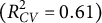
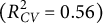
By applying the NV-Embed 200 component model using post-lasso learners onto the human-perception subset of the data, we see that human perceptions (
$R^2_{Y_{HU}} = 0.61$
 ) are explained comparably, even marginally superior to the AI perceptions (
$R^2_{Y_{AI}} = 0.56$
) are explained comparably, even marginally superior to the AI perceptions (
$R^2_{Y_{AI}} = 0.56$
 ), and then the validity measure remain weakly explained (
$R^2_{X} = 0.11$
), and then the validity measure remain weakly explained (
$R^2_{X} = 0.11$
 ; see Table 2 and Figure 4). Percentage of mediated accuracy was very large for both human and AI perceptions, at 112.6% (exceeding 100% due to stochastic fluctuations in the cross-fitting procedure; see Figure 4) and 85.9%, respectively. Importantly, the direct effect between humans perception of social class and the social class validity became non-significant after controlling for the cues (
$\check {\beta } = -0.03, \ SE = 0.02, \ z = -1.45, \ 95\% \text {CI} = [-0.076, 0.011], \ p = 0.15$
; see Table 2 and Figure 4). Percentage of mediated accuracy was very large for both human and AI perceptions, at 112.6% (exceeding 100% due to stochastic fluctuations in the cross-fitting procedure; see Figure 4) and 85.9%, respectively. Importantly, the direct effect between humans perception of social class and the social class validity became non-significant after controlling for the cues (
$\check {\beta } = -0.03, \ SE = 0.02, \ z = -1.45, \ 95\% \text {CI} = [-0.076, 0.011], \ p = 0.15$
 ). For AI perception, the direct effect was small but significant (
$\check {\beta } = 0.03, \ SE = 0.01, \ z = 4.63, \ 95\% \text {CI} = [0.02, 0.05], \ p < 0.001$
). For AI perception, the direct effect was small but significant (
$\check {\beta } = 0.03, \ SE = 0.01, \ z = 4.63, \ 95\% \text {CI} = [0.02, 0.05], \ p < 0.001$
 ) Furthermore, the covariation between humans and AI perception was reduced by 51.2% by controlling for these 200 principal components, indicating that the current cue set well explains the cues that used by both humans and AI, but do not fully explain their shared use. On a similar note, the policy similarities were fairly high between humans and AI (
$G = 0.88$
) Furthermore, the covariation between humans and AI perception was reduced by 51.2% by controlling for these 200 principal components, indicating that the current cue set well explains the cues that used by both humans and AI, but do not fully explain their shared use. On a similar note, the policy similarities were fairly high between humans and AI (
$G = 0.88$
 ), and were a touch lower for the AI and humans in terms of the validity measure (G = 0.75 and 0.71, respectively). On a similar note to the PoMAs, only small amounts of residual correlation remains (
$C = 0.05$
), and were a touch lower for the AI and humans in terms of the validity measure (G = 0.75 and 0.71, respectively). On a similar note to the PoMAs, only small amounts of residual correlation remains (
$C = 0.05$
 and
$C = 0.01$
and
$C = 0.01$
 for AI and humans, respectively).
Decomposition of accuracy: OLS total effects and DML direct effects for human and AI judgments

Table 2 Long description
The table is divided into three sections.
Panel A: Total effects (O L S). Columns include Path, beta, S E, t, 95% C I, and n.
* Path X to A I: beta 0.239, S E 0.010, t 24.02***, C I [0.220, 0.259], n 9,513.
* Path X to H U: beta 0.255, S E 0.041, t 6.16***, C I [0.174, 0.336], n 547.
* Path H U to A I: beta 0.669, S E 0.032, t 21.02***, C I [0.607, 0.732], n 547.
Panel B: Direct effects (D M L). Columns include Path, beta-check, S E, z, 95% C I, and P o M A.
* Path X to A I: beta-check 0.034, S E 0.007, z 4.63***, C I [0.019, 0.048], P o M A 85.9%.
* Path X to H U: beta-check minus 0.032, S E 0.022, z minus 1.45, C I [minus 0.076, 0.011], P o M A 112.6%.
* Path H U to A I: beta-check 0.327, S E 0.061, z 5.35***, C I [0.207, 0.446], P o M A 51.2%.
Panel C: Model performance. Columns include Outcome, Feat., R-squared C V, R-squared I S, C, and G.
* Outcome X: Feat. 160/200, R-squared C V 0.112, R-squared I S 0.145.
* Outcome A I: Feat. 193/200, R-squared C V 0.560, R-squared I S 0.580, C 0.049, G 0.749.
* Outcome H U: Feat. 131/200, R-squared C V 0.605, R-squared I S 0.798, C 0.010, G 0.709.
* H U to A I Relationship: C 0.156 super a, G 0.877 super b.
Note: X represents validity measure, A I represents A I judgment, and H U represents human judgment. Asterisks indicate p < 0.001.
Note: Panels decompose accuracy into total (A; OLS) and direct (B; DML) effects, with model fit indices in Panel C. X = validity measure; AI = AI judgment; HU = human judgment. Panel A: OLS total effects. Panel B: DML with LASSO-selected PCs from 186 language features. PoMA = proportion of mediated accuracy. Panel C: post-LASSO estimates with PCs from 4,096-dim NV-Embed. Feat. = number of features selected/total; CV = cross-validation; IS = in-sample. ***
$p <$
 0.001.
$^{a} <$
0.001.
$^{a} <$
 HU–AI residual correlation.
$^{b} <$
HU–AI residual correlation.
$^{b} <$
 HU–AI policy similarity.
The DML-LM decomposing AI and human judgment.
Note: The model displays the results of the DML-LM analysis using 200 principal components (PCs) as cues (Z). The diagram shows the variance in the validity (X) explained by the cues (
$R^2_{CV} = 0.112$
 ), the variance in AI and Human (HU) judgments explained by cues (
$R^2_{CV} = 0.560$
), the variance in AI and Human (HU) judgments explained by cues (
$R^2_{CV} = 0.560$
 and
$0.605$
and
$0.605$
 , respectively), and the direct effects after accounting for the cues. The percentages represent the proportion of mediated accuracy (PoMA). The values in parentheses below each principal component (e.g., PC3) correspond to the post-LASSO coefficients for the validity measure (X), AI judgments, and Human (HU) judgments, respectively. aWe caution against over-interpreting the magnitude of this percentage exceeding 100%. As the direct effect approached zero, stochastic fluctuations inherent to the cross-fitting procedure in double machine learning likely resulted in a slightly negative, albeit non-significant, coefficient estimate. Thus, we interpret this simply as evidence that the cue set and modeling technique effectively captured the entirety of the mediated effect, treating the excess as statistical noise.

Figure 4 Long description
The diagram is structured with three main horizontal sections.
On the far left, a circle labeled epsilon sub X points to a square labeled X, which has a value R super 2 sub C V equals 0.112 below it.
In the center is a large vertical rectangle containing a list of P C s (Principal Components) with three numerical values in parentheses below each. From top to bottom, the list includes P C 3, P C 2, P C 4, P C 5, P C 6, P C 15, P C 14, P C 12, P C 13, P C 47, P C 10, P C 18, P C 17, P C 21, and P C 106, ending with a note stating 200 Total P C s (X A I H U). To the left of this box, an arrow labeled m sub 0 hat (Z) points toward X. To the right of the box, lines converge into two functions: g sub 01 hat (Z) and g sub 02 hat (Z).
On the right side, g sub 01 hat (Z) points to a square labeled A I (R super 2 sub C V equals 0.560), and g sub 02 hat (Z) points to a square labeled H U (R super 2 sub C V equals 0.605). Above A I is a circle labeled epsilon sub A I, and below H U is a circle labeled epsilon sub H U. A vertical double-headed arrow between A I and H U is labeled 0.327 (51.2%).
Three long curved arrows connect the left and right sides. The top arrow from epsilon sub X to epsilon sub A I is labeled 0.034 (85.9%). The bottom arrow from epsilon sub X to epsilon sub H U is labeled minus 0.032 (112.6% super a). A third curved arrow on the far right connects epsilon sub A I and epsilon sub H U.
5.2.2 Micro-level analysis: Deconstructing judgment in the DML-LM
To understand the cue utilization and validity of the judgment processes of the AI and human raters, we investigated the post-lasso cue utilization and validity coefficients. In particular, the top nine coefficients for each of the validity, human, and AI measures with the largest magnitude were rank ordered, selected, and then visualized, resulting in a set of 15 unique principal components.
Qualitative interpretation of valid and utilized components: Components 2–5 were the variables with largest post-lasso coefficients for all three of social class validity, AI-perceived social class, and human-perceived social class. Based on the Extreme-3-Topic-Word-Clouds, PC2 and 3 appear to measure misspellings (e.g., wood, wen, wont, woud, illegible fiche), and also football, associated with lower social class validity and perception, versus teaching (e.g., teacher, teaching, and class), is associated with higher perceived social class.
PC4 appears to differentiate between traditionally male and female interests. At the high end of PC4, we see football again, which is paradoxically associated with both low and high perceived social class (e.g., manchester, cricket, footballer topic was high in perceived social class, but scotland, football, play, was associated with lower social class perceptions). For traditionally female interests, we see nursing, hospital ward, female, daughter, babies, doctor, and so on. These topics were associated with higher perceived social class. Although PC4 globally was related to social class validity, these topics in particular were primarily related to perceptions of social class.
At the low end of PC5, we see topics that are associated with high levels of social class involving planes or being an air hostess, whereas staying home and being “maried” (poor spelling), with boys or girls and children was associated with lower perceived social class. Thus, this component appears to contrast stay-at-home responsibilities versus being an airline professional, and paradoxically, even though there were illegible fiches involved, university was also mentioned, and thus was still associated with higher levels of social class validity and perception.
Other interesting themes that emerge include college, tennis, racing, ponies, stables, horses, police, meals, dogs, dancing, ballet, and films, for instance, appear to be associated with higher levels of social class, whereas goals (perhaps related to football), and a symphony of basic vocabulary (male, female, boy, girl, army, wife, children, school pet, and mum), and also specific professions (lorry driver, train stations) and, perhaps paradoxically, aspirational living (leading good, better pay, leading a good life) appear to be associated with lower levels of social class. In particular, the particularly valid signals for low social class seem to be related to poor grammar, whereas the particularly valid signals for social class appear to be higher culture activities (ballet, horse riding), and being a teacher, university, or being an airline professional. These results do not claim to be exhaustive, but rather a mere lens into some of the dominant topics that emerge at high and low levels of social class validity and perception. For a full list of coefficients for the top 15 unique components, see Table 3. Figure 5 provides a visualization of word clouds based on different components, along with a UMAP+HDBSCAN visualization of topic clusters with lines connecting the highest and lowest scores for each topic clusters based on each of the top 15 PCs to help visualize the general effect of each component.
Principal component predictors of social class: Validity and judgment coefficients

Table 3 Long description
The table contains six columns: P C, Model, beta, S E, t, and 95% C I. Data is grouped by Principal Component (P C) identifiers.
* P C 3: Validity beta minus 0.127, t minus 13.15. A I beta minus 0.376, t minus 58.51. Human beta minus 0.385, t minus 11.74.
* P C 2: Validity beta minus 0.080, t minus 8.21. A I beta minus 0.293, t minus 43.32. Human beta minus 0.428, t minus 12.40.
* P C 4: Validity beta 0.125, t 12.91. A I beta 0.280, t 42.13. Human beta 0.319, t 9.20.
* P C 5: Validity beta minus 0.107, t minus 11.03. A I beta minus 0.153, t minus 22.62. Human beta minus 0.305, t minus 8.85.
* P C 6: Validity is blank. A I beta 0.119, t 17.60. Human beta 0.224, t 6.57.
* P C 15: Validity beta 0.070, t 7.13. A I beta 0.143, t 21.17. Human beta 0.148, t 4.31.
* P C 14: Validity beta 0.072, t 7.42. A I beta 0.079, t 11.67. Human beta 0.130, t 3.75.
* P C 12: Validity beta 0.066, t 6.81. A I beta 0.101, t 14.94. Human beta 0.154, t 4.44.
* P C 13: Validity is blank. A I beta minus 0.017, t minus 2.50. Human beta minus 0.151, t minus 4.36.
* P C 47: Validity is blank. A I beta minus 0.119, t minus 17.66. Human is blank.
* P C 10: Validity beta minus 0.056, t minus 5.74. A I beta minus 0.100, t minus 14.82. Human beta minus 0.076, t minus 2.19.
* P C 18: Validity beta 0.066, t 6.85. A I beta 0.044, t 6.50. Human beta 0.104, t 3.00.
* P C 17: Validity is blank. A I beta minus 0.086, t minus 12.76. Human beta minus 0.088, t minus 2.54.
* P C 21: Validity is blank. A I beta 0.085, t 12.58. Human beta 0.103, t 2.97.
* P C 106: Validity and A I are blank. Human beta minus 0.085, t minus 2.46.
All reported t-values are statistically significant at p less than 0.05, p less than 0.01, or p less than 0.001 levels as indicated by asterisks.
Note: Post-LASSO coefficients from principal component analysis. Validity = social class; AI = AI judgment; Human = human judgment. Dashes indicate predictors not selected by LASSO. ***p
$<$
 0.001, **p
$<$
0.001, **p
$<$
 0.01, and *p
$<$
0.01, and *p
$<$
 0.05.
0.05.
Interpreting social class perception: UMAP visualization of essay topic clusters.
Note: 3D UMAP projection of essay embeddings, clustered into topics via HDBSCAN. Cluster colors indicate the level and consensus (i.e., agreement between social class validity, AI, and human ratings) of social class judgments, as detailed in the legend. Left: For each of the 15 predictive principal components (PCs), the corresponding word cloud is generated from the combined content of the three lowest-scoring (right) and three highest-scoring (left) topic clusters. Lines then connect each PC to its single highest- and lowest-scoring cluster on the plot.

Figure 5 Long description
The left panel contains a vertical list of 15 P C labels (P C 3 down to P C 106) with numerical values. Each label is paired with two word clouds: a blue-text cloud on the left and a red-text cloud on the right. For example, P C 3 shows football and team in blue versus teacher and teaching in red. P C 2 shows wood and female in blue versus male and street in red.
The right panel is a 3D U M A P scatter plot with axes labeled U M A P 1 (4 to 10), U M A P 2 (4 to 11), and U M A P 3 (5 to 12). The plot contains numerous overlapping spheres representing topic clusters. Black lines with arrows connect specific P C labels (such as P C 12, P C 18, P C 5, P C 3, and P C 15) to specific spheres within the 3D space.
A legend in the top-right corner defines the sphere colors based on social class judgment consensus:
* Dark red: Consensus high
* Light red: Some high
* Dark gray: Opposing signals
* Light blue: Some low
* Dark blue: Consensus low
* Light gray: All middle
6 Discussion
6.1 The DML-LM reveals similar kernel-of-truth mechanisms across human and AI perceivers
A central finding of this study is that AI and human judgments of social class are largely anchored to the same kernels-of-truth, and that they have a surprising level of consensus in the way they use cues for perception. The broad levels of consensus aligns with the magnitude reported in recent human–AI comparison literature (e.g., Rathje et al., Reference Rathje, Mirea, Sucholutsky, Rao and Van Bavel2024), but this study helped to illustrate that many cues that inform our perceptions are similar, although not identical. Our results also provide strong evidence for the kernel-of-truth hypothesis (Campbell, Reference Campbell1967), showing how weak signals of an objective validity measure like social class can be magnified by both humans and AI into the large perceptual differences, aligning with social class stereotype accuracy results found in other research (Bjornsdottir, Reference Bjornsdottir2025; Eagly & Hall, Reference Eagly and Hall2025).
6.2 Re-evaluating “unmodeled knowledge” in the age of big data
The high proportion of judgmental accuracy explained by our framework challenges the long-held role of “unmodeled knowledge” in person perception. Historically, large residuals in accuracy models have been interpreted as evidence that perception is a largely ambiguous and intuitive process that defies quantification, a view advanced across phenomenological, qualitative, and critical traditions (e.g., Dreyfus, Reference Dreyfus1972; Merleau-Ponty, Reference Merleau-Ponty2012; Polkinghorne, Reference Polkinghorne1995). Our results, however, suggest that this explanatory gap may be an artifact of prior measurement limitations rather than an indication of an inherently unmeasurable process. This aligns with Funder’s (Reference Funder1995) Realistic Accuracy Model, which posits that accuracy depends on the detection of valid, context-sensitive cues. While previous research has highlighted the immense difficulty of exhaustively coding such cues (e.g., Borkenau et al., Reference Borkenau, Mosch, Tandler and Wolf2016) and often only found larger effect sizes in experimental settings (see Karelaia & Hogarth, Reference Karelaia and Hogarth2008), our findings demonstrate that high-dimensional methods can successfully capture this complexity, reframing “unmodeled knowledge” as previously under-measured knowledge.
Furthermore, our findings speak to Meehl’s (Reference Meehl1990) influential critique that researchers should prioritize the magnitude of effects over mere statistical significance. The present study identified numerous significant predictors, yet our recommended approach emphasizes examining the most dominant and interpretable components (e.g., PC2, 3, 4, and 5) that explain the most variance and carry the strongest, most theoretically coherent weights. By concentrating on these substantial effects, we refrain from over-interpreting minor cues whose statistical significance may be an artifact of high statistical power, thereby addressing Meehl’s concern.
This approach represents a paradigm that differs from building theory upon isolated and often weak effects. Instead, we first optimize for prediction, allowing complex signals to emerge from the data in an unsupervised manner. We acknowledge that these predictively strong components are composite measures that can be difficult to interpret, as evidenced by some incoherence in the thematic visualizations. Therefore, our interpretation of the dominant themes is offered as a partial but principled account of the model’s primary drivers. This allows us to begin with the premise that the phenomenon is complex, and from there, identify the powerful signals that provide a robust, data-driven foundation for theory. This is a step toward a more meaningful understanding of the mechanisms of perception.
6.2.1 The bias–variance tradeoff in a text perception setting
Our findings provide a practical illustration of the bias–variance tradeoff with somewhat surprising results. Highly flexible, low-bias models like XGBoost demonstrated poor generalization due to high variance; they fit noise in the training data, as evidenced by negative cross-validated
$R^2$
 scores indicating predictions worse than the mean. Similarly, unregularized OLS on high-dimensional feature sets failed due to extreme overfitting. This was contrary to our initial ideas that flexible machine learning models would provide superior performance in such a high-dimensional space, such as that of the 4,096 dimensions. In contrast, regularized linear models (lasso and ridge) succeeded by introducing a small amount of bias to substantially reduce variance. This constraint on coefficient estimates prevented overfitting and yielded far superior predictive performance on new data. For psychological datasets like ours, characterized by moderate size, inherent noise, and class imbalance, the stability and generalizability offered by regularization proved more effective than the high flexibility of more complex models. This suggests that high-dimensional language representations combined with PCA may perform particularly well with linear models, despite an initial sentiment that a flexible model may be the best option.
Contrary to the assumption that high-dimensional tasks require complex architectures, OLS utilizing PCA-reduced NV-Embed embeddings yielded results nearly identical to the top-performing regularized models. While Lasso offers the distinct advantage of sparsity (enhancing interpretability by zeroing out irrelevant components), the efficacy of OLS highlights that aggressive dimensionality reduction can be as effective as regularization. This finding serves as a reminder that in the bias–variance tradeoff, prioritizing variance reduction (via PCA) can often yield better generalization than increasing model flexibility.
6.2.2 Language model embeddings model text better than LIWC for perception
Consistent with a growing body of research (Koutsoumpis et al., Reference Koutsoumpis, Oostrom, Holtrop, Van Breda, Ghassemi and De Vries2022; Schwartz et al., Reference Schwartz, Eichstaedt, Kern, Dziurzynski, Ramones, Agrawal, Shah, Kosinski, Stillwell, Seligman and Ungar2013), our study confirms that modern language model embeddings significantly outperform traditional dictionary-based methods like LIWC. This performance gap stems from the inherent limitations of LIWC’s static, low-dimensional approach. Unlike embeddings, dictionary methods are not context-aware and cannot capture meaning derived from word co-occurrence, a principle central to distributional semantics (Firth, Reference Firth1957). Furthermore, LIWC’s closed-vocabulary design struggles to model misspellings, grammatical errors, or novel phrases (Schwartz et al., Reference Schwartz, Eichstaedt, Kern, Dziurzynski, Ramones, Agrawal, Shah, Kosinski, Stillwell, Seligman and Ungar2013), while embeddings leverage the high-dimensional representations that have long been recognized as essential for robust text analysis (Landauer & Dumais, Reference Landauer and Dumais1997). The practical consequence of these limitations is a significant loss of predictive power, a conclusion supported by findings that only a small fraction of LIWC variables validly predict ground-truth personality traits (Koutsoumpis et al., Reference Koutsoumpis, Oostrom, Holtrop, Van Breda, Ghassemi and De Vries2022). While LIWC’s simplicity ensures its value as a baseline, our results underscore that achieving a more powerful and valid understanding of language now necessitates the adoption of these more sophisticated techniques.
Significant performance variability exists even among different language embedding models. For instance, the smaller miniLM model demonstrated commendable performance, achieving approximately four-fifths of the predictive accuracy of the state-of-the-art NV-Embed model. The superior performance of NV-Embed is likely attributable to more advanced mechanisms, such as its novel latent attention mechanism and larger parameter count, which theoretically enable it to capture more nuanced linguistic complexities. Beyond quantitative metrics, our own qualitative observations also suggested that the thematic topics generated from the NV-Embed embeddings were more coherent and specific than those from the MiniLM model. This highlights a critical area for future research: systematically investigating how different embedding architectures, sizes, and training objectives influence their capacity to identify psychologically relevant constructs.
6.3 Broader implications and future directions
6.3.1 Advancing perception theory with multimodal data
The present study demonstrates how textual cues reveal a “kernel-of-truth” in social class stereotypes. However, a comprehensive understanding of social perception requires moving beyond a single modality. The DML-LM introduced here is modality-agnostic, making it ideal for building a more holistic model of perception by integrating multiple channels of information such as text, audio, and video.
This direction builds on a rich tradition in lens model research, which has long shown that accuracy varies across different information channels (Osterholz et al., Reference Osterholz, Breil, Nestler, Back, Letzring and Spain2021). For social class, this means modeling the potent influence of visual and auditory cues. Visual information from the face, for example, is strongly associated with class perceptions via stereotypes linking traits like competence and warmth to higher social standing (Bjornsdottir & Rule, Reference Bjornsdottir and Rule2017). Similarly, the voice acts as an “auditory face,” with speech characteristics like accent and pitch serving as powerful, if stereotypical, markers of class (Kachel et al., Reference Kachel, Simpson and Steffens2018). Beyond social class, this approach can clarify how other traits, like extraversion, are expressed through a combination of controlled cues (e.g., stylish dress) and automatic ones (e.g., expressive body movements and cheerful voice) across different modalities (Hirschmüller et al., Reference Hirschmüller, Egloff, Nestler and Back2013). Applying the DML-LM to such high-dimensional, multimodal data would allow researchers to model how cues in one modality (e.g., a confident tone of voice) interact with or override cues in another (e.g., hesitant language). This would not only enable a direct comparison of how humans and AI weigh different information streams but also fuel the development of richer, more ecologically valid theories of perception that embrace the reality that trait expression is fundamentally context-dependent (Fleece & Teglasi, Reference Fleece and Teglasi2024).
6.3.2 Modeling informant discrepancy
In a similar way how different modalities matter, researchers often grapple with why different informants, such as parents and teachers, provide divergent ratings of the same person. For instance, fewer than half of children were classified similarly by both parents and teachers on key traits like behavioral inhibition (Fleece & Teglasi, Reference Fleece and Teglasi2024). Such discrepancies arise from informant-specific effects, where the perceived relationships between traits can be an artifact of a single rater’s perspective (Biesanz & West, Reference Biesanz and West2004). The DML-LM is uniquely positioned to address this challenge by moving beyond simple comparison. By treating each informant as a “perceiver,” the DML-LM can use high-dimensional behavioral data (e.g., narrative accounts) to model their distinct judgment policies. This allows for a precise quantification of cue utilization variability across informants, where one informant weighs a specific cue heavily while another discounts it (Hirschmüller et al., Reference Hirschmüller, Egloff, Nestler and Back2013).
6.3.3 A new frontier for auditing high-stakes AI
Modeling informant discrepancy between humans and AI has never been more important, especially with AI beginning to encroach on high-stakes frontiers. For example, AI ought to be audited for the ways in which it uses cues in patient data when compared to expert physicians to reveal areas of discrepancy that may spur downstream inequalities (Ratwani et al., Reference Ratwani, Sutton and Galarraga2024). In human resources, AI-powered hiring tools have been deployed and leading to biased screening outcomes, and thus deserve auditing and understanding of the differential cue use and validity (Tilmes, Reference Tilmes2022). In finance, this framework is especially salient. For example, Fuster et al. (Reference Fuster, Goldsmith-Pinkham, Ramadorai and Walther2022) studied the U.S. mortgage market and found that shifting from traditional logistic regression models to Random Forest models for predicting a person’s probability of defaulting resulted in disproportionately disadvantaged Black and Hispanic borrowers, increasing their interest rate by nearly double for Black and Hispanic borrowers compared to White non-Hispanic borrowers. Such outcomes may arise from the model’s increased flexibility and enhanced ability to triangulate protected characteristics from permissible data. Through the DML-LM, researchers can go beyond the identification of the presence of bias, and investigate how machine learning models amplify biases, increasing transparency in the high-stakes frontiers like healthcare, employment, and finance.
6.3.4 Experimental validation through mechanistic interpretability
While the DML-LM provides a powerful diagnostic lens, the next frontier is to move from correlational observation to causal validation. This requires delving into mechanistic interpretability to reverse-engineer a model’s internal computations. A primary obstacle is polysemanticity, where neurons represent multiple unrelated concepts due to superposition, a compression strategy where models encode more features than they have neurons (Elhage et al., Reference Elhage, Hume, Olsson, Schiefer, Henighan, Kravec, Hatfield-Dodds, Lasenby, Drain, Chen, Grosse, McCandlish, Kaplan, Amodei, Wattenberg and Olah2022). Indeed, we see polysemanticity in our current results, where different principal components appear to be tapping into the same phenomenon (e.g., football for PC3 and PC4).
To overcome this, our framework can be integrated with techniques like sparse autoencoders, which decompose a model’s internal activations into more monosemantic (single-concept) features that are functionally equivalent to the “cues” in our model (Cunningham et al., Reference Cunningham, Ewart, Riggs, Huben and Sharkey2024). Once these latent features are identified, their causal role can be experimentally tested. For instance, using activation patching, a researcher could directly manipulate the model’s internal state to activate a specific feature (e.g., “formal professional language”) and measure its direct impact on the final judgment. If the manipulation reliably alters the outcome, it provides strong causal evidence that the feature is a mechanistic driver of the model’s perception. This approach enables the automated discovery of entire causal circuits within the model, moving far beyond simple cue-judgment correlations.
6.4 Limitations
While the present study introduces a robust framework for analyzing high-dimensional perception, several limitations should be acknowledged. First, the analyses were conducted on a historical dataset of essays from the 1960s. Although this provided a unique opportunity to examine perceptions of social class, the language, societal norms, and class structures of that era may not be directly generalizable to contemporary contexts. The validity variable itself, a five-point measure of the father’s occupational social class, was coarse and imbalanced, which likely constrained the predictive performance of all models and may have particularly disadvantaged complex, high-variance models like XGBoost that are sensitive to noisy data.
Second, a central challenge in this work is the interpretability of high-dimensional representations. While we demonstrated a viable approach for decoding principal components by combining topic modeling and extreme group analysis, this process remains inherently qualitative and requires careful consideration. A critical direction for future research is to develop and validate more systematic and rigorous methodologies for interpreting the otherwise opaque components derived from dimensionality reduction techniques. Establishing best practices for this process is essential for moving from statistical explanation to true theoretical understanding.
Third, while our high-dimensional text representations capture a vast amount of information, there are still other domains of perception left unmeasured. One primary variable is time. For instance, Huang et al. (Reference Huang, Prijatelj, Dulay and Scheirer2023) found reaction time and judgment confidence during perception to be a relevant cue that improved classification performance. Future studies ought to examine how the DML-LM could capture time effects, reputation effects (e.g., McAbee & Connelly, Reference McAbee and Connelly2016), and accuracy outside of a zero-acquaintance setting.
7 Conclusion
This study introduced the DML-LM as a novel framework for deconstructing and comparing the architecture of perception in the age of artificial intelligence. An application of this framework to the judgment of social class from text challenges a simple narrative of AI as an alien intelligence, revealing instead a remarkable degree of overlap with human perception. The findings indicated that both AI and human judgments are anchored to the same potent, thematic “kernels of truth” embedded in language.
The critical distinction, however, lies not in what is perceived but in how. The AI’s judgment policy was found to be substantially less sparse, systematically integrating a much broader array of textual cues than the more heuristic and parsimonious model employed by humans. While both perceivers amplify subtle, real-world patterns into powerful and potentially discriminatory heuristics, the AI’s use of a wider set of cues results in a particularly rigid and impactful form of this amplification. The implication of this finding is profound: as AI systems are increasingly integrated into high-stakes domains, it is insufficient to know that they are often accurate. The frameworks presented here provide a necessary diagnostic lens, revealing that even when an algorithm’s perception closely mirrors our own, subtle but significant differences in its process can lead to large and consequential differences in its real-world impact. This research represents a critical step toward a more nuanced understanding of AI and the development of more accurate, fair, and transparent decision-making systems.
Data availability statement
The code used for the analyses in this study is available in the Open Science Framework repository at https://osf.io/wrn6e/. The analyses were conducted using the HAAM package, which is available on both GitHub (https://github.com/raymondli-me/haam) and OSF.
Acknowledgments
This article is based on the first author’s master’s thesis, submitted to the University of British Columbia. During the preparation of this work, the authors used ChatGPT 4o and o1 (https://chat.openai.com/), Claude Opus 4 (https://claude.ai), and Gemini 2.5 Pro (https://gemini.google.com) in order to improve the clarity of writing, to assist with producing figures, and to help produce statistical code. After using these tools, the authors reviewed and edited the content and take full responsibility for the content of the publication. This manuscript is part of the special section, Integrating and Analyzing Complex High-Dimensional Data in Social and Behavioral Sciences Research. We extend our heartfelt gratitude to the co-Guest Editors, Drs Katrijn Van Deun and Eric Lock, as well as the reviewers for their invaluable and insightful feedback, which significantly enhanced this article.
Funding statement
Preparation of this manuscript was supported by the Social Sciences and Humanities Research Council (SSHRC) of Canada Grant 435-2020-0203 to J.C.B.
Competing interests
The authors declare no competing interests.
Ethical standards
This study was approved by the Behavioural Research Ethics Board of the University of British Columbia (No. H20-01189). Informed consent was obtained from all participants.
Informed consent
Informed consent was obtained from all participants.
Appendices
Appendix A: Derivation of the double machine learning lens model
Step 1: Observed variables We represent the validity
$(X)$
 and judgment
$(Y)$
and judgment
$(Y)$
 with cross-fit predictions and residuals:

where
$\hat {X} \approx \hat {m}_0(Z)$
 and
$\hat {Y} \approx \hat {g}_0(Z)$
and
$\hat {Y} \approx \hat {g}_0(Z)$
 , each estimated via cross-fitting over covariates Z. Under double machine learning, the Neyman-orthogonal structure ensures that final correlation estimates remain robust to potential estimation errors from the regularization of
$\hat {m}_0$
, each estimated via cross-fitting over covariates Z. Under double machine learning, the Neyman-orthogonal structure ensures that final correlation estimates remain robust to potential estimation errors from the regularization of
$\hat {m}_0$
 and
$\hat {g}_0$
and
$\hat {g}_0$
 .
.
Step 2: Covariance decomposition

Step 3: Variance decomposition

Define the cross-fit coefficient:

If
$\hat {X}$
 and
$e_X$
and
$e_X$
 are not orthogonal, we set

Then
$\mathrm {Var}(\hat {X}) = (R_X^2 - E_X)\,\mathrm {Var}(X)$
 and
$\mathrm {Var}(e_X) = (1 - R_X^2)\,\mathrm {Var}(X).$
and
$\mathrm {Var}(e_X) = (1 - R_X^2)\,\mathrm {Var}(X).$

Step 4: Modeled and residual covariances

We define cross-covariance parameters:

They may be non-zero for flexible ML estimators.
Step 5: Overall achievement The correlation
$r_a = \mathrm {Cor}(X,Y)$
 can be written as

which is often expanded as

If the cross-covariances vanish and
$E_X=E_Y=0$
 (pure OLS), it reduces to
$r_a = G\,\sqrt {R_X^2}\,\sqrt {R_Y^2} + C\,\sqrt {1 - R_X^2}\,\sqrt {1 - R_Y^2}.$
(pure OLS), it reduces to
$r_a = G\,\sqrt {R_X^2}\,\sqrt {R_Y^2} + C\,\sqrt {1 - R_X^2}\,\sqrt {1 - R_Y^2}.$

Step 6: Debiased unmodeled correlation Under cross-fitting with standardized residuals, C corresponds to the double-machine-learning estimator:

providing an unbiased estimate of the residual relationship between X and Y after controlling for high-dimensional Z.
Appendix B: Large language model configuration and prompting protocol
B.1 Model configuration
For the automated generation of social class ratings, we employed the Qwen/Qwen2.5-32B-Instruct-AWQ large language model, a 32-billion parameter instruction-tuned model. The model was accessed through the vLLM inference library with the following technical specifications:
-
• Quantization: Activation-aware weight quantization (AWQ) with 16-bit floating-point precision (float16) for computational efficiency.
-
• Context length: Maximum of 2,048 tokens.
-
• Hardware distribution: Two GPUs with tensor_parallel_size=2.
-
• Memory utilization: 80% GPU memory limit.
-
• Sampling temperature: 0.1 for semi-deterministic outputs.
-
• Maximum response tokens: 200 per generation.
-
• Batch processing: Essays processed in batches of 100 for computational throughput optimization.
-
• Optimization settings: Triton Flash Attention and torch.compile disabled for reproducibility.
B.2 Prompting protocol
Each essay was evaluated using a carefully structured multi-part prompt based on an adaptation of the MacArthur Scale of Subjective Social Status (Adler et al., Reference Adler, Epel, Castellazzo and Ickovics2000). The prompt instructed the model to place the child’s family on a 10-rung societal ladder and return the rating as a JSON object.
System message:

User message template:

Example model response:

Appendix C: Human perceiver data collection
C.1 Participant recruitment and demographics
In 2021, we recruited 600 participants from the United Kingdom through the Prolific online research platform to evaluate the perceived social class of essays written by 11-year-old participants in the 1958 National Child Development Study (NCDS) (Power & Elliott, Reference Power and Elliott2006; Centre for Longitudinal Studies, 2025). The study protocol received approval from the University of British Columbia’s Behavioral Research Ethics Board (BREB No. H20-01189).
Sample characteristics:
-
• Gender distribution: 304 female participants.
-
• Age: Mean = 37 years ( $SD = 13.06$
 ), Range = 18–76 years.
 -
• Nationality: All current or former U.K. residents.
-
• Ethnic composition:
-
– European ancestry: $n = 493.$
-
– East Asian: $n = 15.$
-
– Southeast Asian: $n = 9.$
-
– South Asian: $n = 31.$
-
– Middle Eastern: $n = 4.$
-
– Other backgrounds: $n = 48.$
-
-
• Compensation: £6.91 per participant.


C.2 Data collection procedure
The data collection protocol consisted of the following steps:
-
1. Participants completed a demographic questionnaire.
-
2. Participants viewed an informational video about the NCDS to provide contextual understanding.
-
3. Each participant evaluated 10 randomly assigned essays.
-
4. Participants rated the perceived social class of each essay writer’s family using an adapted MacArthur Scale.
MacArthur scale instructions: Participants were presented with a ladder image and the following prompt:
“Imagine that this ladder pictures how society is set up. At the top of the ladder are the people who are the best off—they have the most money, the highest amount of schooling, and the jobs that bring the most respect. At the bottom are people who are the worst off—they have the least money, little or no education, no job, or jobs that no one wants or respects. Where do you think the family of the person who wrote this essay would be on this ladder?”
C.3 Data processing and sample size determination
The original dataset comprised 10,511 essays written in 1969 by 11-year-old NCDS participants. From this corpus, 600 essays were randomly selected for human evaluation. Of these, 547 essays had corresponding social class validity data available for analysis.
Averaging across human raters: Each essay received ratings from an average of 10 different perceivers. The final perceived social class score for each essay was calculated as the mean of these individual ratings, resulting in 547 essays with averaged human social class judgments.
Statistical power: With a sample size of 547 essays, our study achieved 80% power to detect correlations of
$r \geq 0.12$
 between human ratings and social class validity measures, ensuring adequate sensitivity for detecting even small effect sizes in the accuracy of social class perception.
Appendix D: Distribution of social class measures
Distributions of human judgments, AI judgments, and social class validity.
Note: The figure displays histograms for the three key variables in the study. Panel (a) shows the distribution of social class ratings from human perceivers (
$n = 547$
 ) on a 10-point scale. Panel (b) shows the distribution of social class ratings from the AI model for all essays (
$n = 9,513$
) on a 10-point scale. Panel (b) shows the distribution of social class ratings from the AI model for all essays (
$n = 9,513$
 ) on the same 10-point scale. Panel (c) shows the distribution of the ground-truth social class validity measure, based on the reverse-coded 5-point Registrar General’s Social Class scale (
$n = 9,513$
) on the same 10-point scale. Panel (c) shows the distribution of the ground-truth social class validity measure, based on the reverse-coded 5-point Registrar General’s Social Class scale (
$n = 9,513$
 ). Dashed vertical lines indicate the mean for each distribution.

Figure D1 Long description
The figure consists of three side-by-side histograms.
Panel a, titled Human Rating, uses a horizontal x-axis from 0 to 10 and a vertical y-axis for Frequency from 0 to 120. The data shows a normal distribution centered around a mean of 5.52, indicated by a vertical dashed line. A box in the top right lists M = 5.52, S D = 0.89, and n = 547.
Panel b, titled A I Rating, uses a horizontal x-axis from 0 to 10 and a vertical y-axis for Frequency from 0 to 3500. The distribution is bimodal with a primary peak between 4 and 5 and a secondary peak at 3. A vertical dashed line marks the mean at 4.45. A box in the top right lists M = 4.45, S D = 1.36, and n = 9,513.
Panel c, titled Social Class, uses a horizontal x-axis from 0 to 10 and a vertical y-axis for Frequency from 0 to 6000. Note text indicates a scale of 1 to 5. The distribution is highly concentrated between 2 and 4, peaking sharply at 3. A vertical dashed line marks the mean at 2.92. A box in the top right lists M = 2.92, S D = 0.89, and n = 9,513.

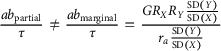


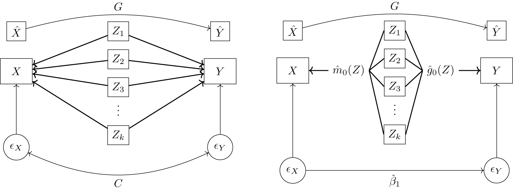


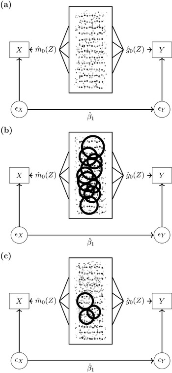
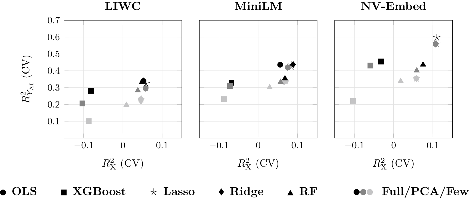


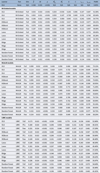
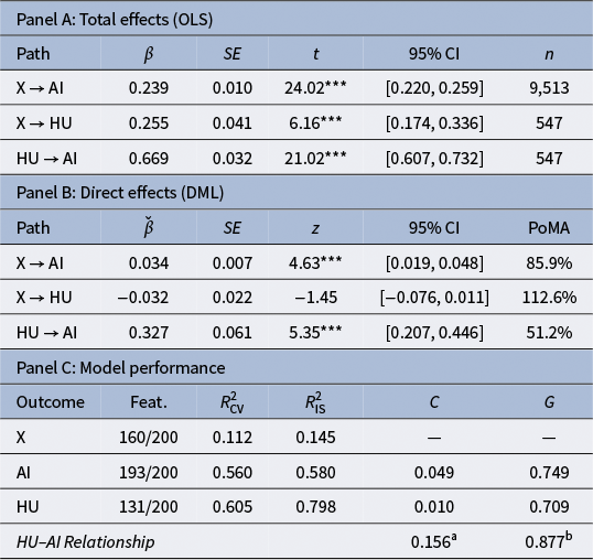
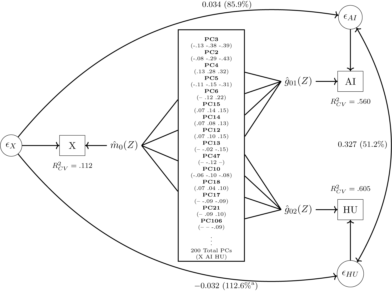


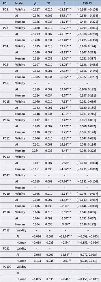
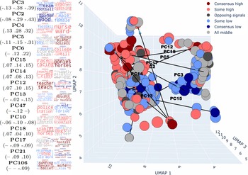
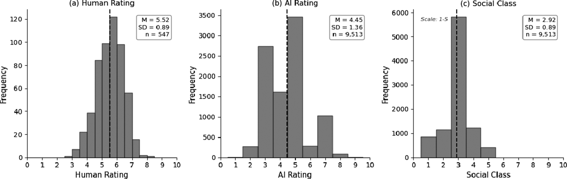


 Open access

