


1. Introduction
The Blue Lias Formation (uppermost Triassic and Lower Jurassic) comprises alternating centimetre- to metre-scale beds of homogeneous light grey limestone; light grey marl associated with homogeneous light grey limestone nodules; dark grey marl; and black, organic-rich laminated shales associated with nodules of very dark grey laminated limestone (Hallam, Reference Hallam1960; Weedon, Reference Weedon1986). Recently, it was demonstrated that hiatuses are prevalent throughout the formation in southern Britain, as inferred from field observations and from graphic correlation using the locations of numerous ammonite biohorizons (Weedon et al. Reference Weedon, Jenkyns and Page2018). The sedimentary cyclicity in the form of alternating limestones and non-limestones and alternating laminated and homogeneous (bioturbated) microfacies has been well studied (Hallam, Reference Hallam1960, Reference Hallam1964, Reference Hallam1986; Weedon, Reference Weedon1986; Raiswell, Reference Raiswell1988; Weedon et al. Reference Weedon, Jenkyns, Coe and Hesselbo1999, Reference Weedon, Jenkyns and Page2018; Arzani, Reference Arzani2006; Paul et al. Reference Paul, Allison and Brett2008). Here, we reassess the evidence for regular cyclicity and for astronomical or ‘orbital’ forcing of climate in the offshore hemipelagic Blue Lias facies using time-series analysis of high-resolution magnetic susceptibility logs.
There is a tension in some recent cyclostratigraphic studies between the interpretations of the researchers and the long-recognized incompleteness of the stratigraphic record (e.g. Ager, Reference Ager1973, who underscored stratigraphic incompleteness in general compared with the emphasis on stratigraphic continuity by Hilgen et al. Reference Hilgen, Hinnov, Aziz, Abels, Batenburg, Bosmans, de Boer, Hüsing, Kuiper, Lourens, Rivera, Tuenter, Van der Wal, Wotslaw, Zeeden, Smith, Bailey, Burgess and Fraser2015). Interval dating involves estimating the amount of time elapsed between two events, such as biostratigraphic boundaries, when the ‘absolute’ or numerical ages are unknown. With the use of this methodology there has been a tendency for many cyclostratigraphic investigators to assume that a section of particular interest can be considered to be complete (e.g. Ruhl et al. Reference Ruhl, Deenen, Abels, Bonis, Krijgsman and Kürschner2010). Conversely, many authors, notably including Darwin (Reference Darwin1859), have observed that stratigraphic records of evolutionary history are incomplete and some, such as Buckman (Reference Buckman1898, Reference Buckman1902), have convincingly demonstrated that high-resolution biostratigraphy can be used to identify local gaps (Page, Reference Page2017). The incompleteness of the stratigraphic record and its consequences for studies of evolutionary processes are well understood by palaeontologists.
Sadler (Reference Sadler1981) established quantitatively that all sedimentary sections, regardless of the associated environment, are incomplete lithostratigraphically. Analysis of pelagic strata plus numerical modelling emphasized the generality of this observation (Anders et al. Reference Anders, Krueger and Sadler1987; Sadler & Strauss, Reference Sadler and Strauss1990). Sedimentary completeness can only be meaningfully described by reference to a specific time scale (i.e. resolution) of interest (Sadler, Reference Sadler1981). The longer the total time represented by a stratigraphic interval, the lower will be the likely completeness at the selected time resolution (Sadler, Reference Sadler1981; van Andel, Reference Van Andel1981; Anders et al. Reference Anders, Krueger and Sadler1987; Sadler & Strauss, Reference Sadler and Strauss1990).
These ideas lead to a general principle for cyclostratigraphy. Since interval dating from cyclostratigraphy utilizes counts of sedimentary cycles in individual stratigraphic sections, it follows that durations estimated from single sections will nearly always be underestimates. Hence, by combining cycle counts from multiple sections, more reliable interval dating can be obtained than from counts from single sections.
Shaw (Reference Shaw1964) demonstrated that, rather than requiring a perfect knowledge of the ranges of stratigraphically valuable taxa, useful information can be obtained by comparing pairs of sections graphically (i.e. via Shaw plots). Shaw plots for multiple sections can be used to generate composite estimates of biostratigraphic ranges. Furthermore, the slope of the ‘line of correlation’ provides a measure of the relative accumulation rates between localities. However, of more significance here, Shaw plots can also be used to locate stratigraphic gaps at steps in the line of correlation.
An essential aspect of the reassessment of the evidence for astronomical forcing in the hemipelagic Blue Lias Formation is allowance for the presence of numerous stratigraphic gaps in all the sections studied. Hiatuses can cause substantial distortion of the relationship between time and depth or height in stratigraphic sections (Weedon, Reference Weedon2003; Kemp, Reference Kemp2012). Nevertheless, analysis of model time series, with randomly distributed gaps and random amounts of strata missing, has shown that spectral detection of regular cyclicity in the depth domain remains possible when large gaps are widely spaced or the gaps are small relative to the size of regular cycles (Weedon, Reference Weedon1989, Reference Weedon, Einsele, Ricken and Seilacher1991, Reference Weedon2003).
Widely spaced hiatuses can be detected using time-series characteristics in hemipelagic strata via spectrograms obtained from either moving window Fourier analysis (Meyers & Sageman, Reference Meyers and Sageman2004) or by using wavelets (Prokoph & Barthelmes, Reference Prokoph and Barthelmes1996; Prokoph & Agterberg, Reference Prokoph and Agterberg1999). Hiatuses have been located by finding ‘jumps’ in marine strontium isotopes obtained from skeletal calcite, although this requires centimetre-scale sampling (Jenkyns et al. Reference Jenkyns, Jones, Gröcke, Hesselbo and Parkinson2002; McArthur et al. Reference McArthur, Steuber, Page and Landman2016). Aside from the sedimentological evidence described by Weedon et al. (Reference Weedon, Jenkyns and Page2018), hiatus detection within the Blue Lias Formation has relied on high-resolution biostratigraphic studies, including using biohorizons (e.g. Page, Reference Page, Lord and Davis2010 a) or the correlation of stratigraphic or compositional data typically using Shaw plots (Smith, Reference Smith1989; Bessa & Hesselbo, Reference Bessa and Hesselbo1997; Deconinck et al. Reference Deconinck, Hesselbo, Debuisser, Averbuch, Baudin and Bessa2003; Weedon et al. Reference Weedon, Jenkyns and Page2018).
Here, high-resolution logs of volume magnetic susceptibility (vol. MS) from four localities (Fig. 1) are used as proxy time series for inversely varying calcium carbonate contents (Weedon et al. Reference Weedon, Jenkyns and Page2018). In this contribution, the term ‘time series’ is applied in the original formal mathematical sense (Priestley, Reference Priestley1981) to refer to any sequentially ordered discretely observed variable (i.e. regardless of whether the ordering of the data is according to stratigraphic depth/height or time). The four vol. MS logs together span the top of the last stage of the Triassic (Rhaetian) and the whole of the first stage of the Jurassic, the Hettangian (comprising the Tilmanni, Planorbis, Liasicus and Angulata zones), plus the Conybeari Subzone of the succeeding Bucklandi Zone (basal Sinemurian Stage). Note that ammonite zones are used in the sense of ‘chronozones’, as discussed by Page (Reference Page2017).
Localities of the vol. MS time series. The data from St Audries Bay and Quantock’s Head were combined into a composite section for the West Somerset Coast (Weedon et al. Reference Weedon, Jenkyns and Page2018).

After discussion of previous studies (Section 2), the time-series methodology is described in detail (Section 3), including tests for regular cyclicity using both standard (non-Bayesian) spectral analysis and Bayesian probability spectral analysis. Section 4 describes detection of different scales of regular cyclicity in depth, and an astronomical attribution is discussed in Section 5. The next section describes the lithological expression of the different scales of cyclicity, and Section 7 considers the biostratigraphic information and the relationship between biohorizons and time. The positions of the inferred astronomically forced sedimentary cycles are then used to produce local tuned time scales (Section 8). The tuned time scales provide estimates of the minimum duration of individual biohorizons and of the entire Hettangian Stage. Next, by combining the biohorizon positions with the local tuned time scales from three sites, a composite time scale is constructed that incorporates the local stratigraphic gaps (Section 9). It is shown that the estimated minimum duration of the Hettangian from combining data from multiple sections increases compared with that from the local tuned time scales. The resulting estimates differ substantially from the most recently published estimates for the length of the Hettangian Stage (Section 10). The composite time scale is also used to quantify local completeness at the 10 000 year scale and to investigate the relative timing of deposition of black, organic-rich laminated shale at different localities.
2. Previous studies of astronomical forcing of cycles in the Blue Lias Formation and the implications for the duration of the Hettangian Stage
Shukri (Reference Shukri1942) seems to have been the first to consider the possibility that sedimentary cycles in the Blue Lias might have been astronomically driven. Noting that the spacing of the limestone beds increased substantially from the Angulata Zone into the upper Bucklandi Zone at Lyme Regis, and that the cycles were therefore of varying wavelengths, he ruled out forcing by precession. He does not appear to have considered the possibility that increased accumulation rates might explain the changing spacing of the limestones. The alternative possibility is that increased water depths related to sea-level change could have progressively diminished the likelihood of forming storm-influenced hiatuses on the sea floor and thus limited the development of early diagenetic limestone in the upper interval (Waterhouse, Reference Waterhouse1999; Weedon et al. Reference Weedon, Jenkyns and Page2018).
Following the spectral analysis of securely dated Pleistocene deep-sea sediments by Hays et al. (Reference Hays, Imbrie and Shackleton1976), the Croll–Milankovitch Theory of the ice ages was resurrected (e.g. Imbrie et al. Reference Imbrie, Hays, Martinson, McIntyre, Mix, Morley, Pisias, Prell, Shackleton, Berger, Imbrie, Hays, Kukla and Saltzman1984). House (Reference House1985) suggested that, on the assumption that the limestone/mudrock alternations of the Blue Lias could be attributed to astronomical forcing, counts of cycles could be used to refine the geological time scale, essentially following the reasoning of Gilbert (Reference Gilbert1895).
Weedon (Reference Weedon1986) used digitized stratigraphic logs and Walsh spectral analysis to argue that the regular sedimentary cycles in the Blue Lias are explicable in terms of astronomical forcing of climate. However, the spectral analysis used complete logs without allowing for the possibility of changing accumulation rates. The statistical significance of the spectral peaks was tested against a white-noise model (flat spectral background) rather than a more modern approach that would test against a sloping (red-noise) spectral background. Two scales of cyclicity were detected and inferred to relate to obliquity or precession. On the then ‘traditional’ assumption that ammonite zones lasted about 1 million years each, undetected hiatuses implied completeness of 20 to 40 % at the tens of thousands of years scale (Weedon, Reference Weedon1986).
Waterhouse (Reference Waterhouse1999) studied beds 21 to 45 of the Blue Lias Formation (bed numbers of Lang, Reference Lang1924) at Lyme Regis on the Devon/Dorset border, i.e. Conybeari to middle Bucklandi subzones of the Bucklandi Zone (Sinemurian Stage). Regularity was established spectrally using raw periodograms with apparently no attempt to establish the statistical significance of spectral peaks. The interval studied corresponds to that studied by Shukri (Reference Shukri1942) and is characterized by the aforementioned large change in the spacing of the limestones. Waterhouse (Reference Waterhouse1999) inferred regular cycles in palynomorphs, but an absence of regular lithological cyclicity. However, it is likely that the lack of large spectral peaks for the lithostratigraphic data was caused by analysis of non-stationary time series (i.e. in this case, data with large changes in the scales of variation or degree of variability; Weedon, Reference Weedon2003).
Weedon et al. (Reference Weedon, Jenkyns, Coe and Hesselbo1999) obtained a high-resolution log of volume magnetic susceptibility at Lyme Regis with a fixed stratigraphic spacing of measurements at 2 cm at Lyme Regis (as utilized here and by Weedon et al. Reference Weedon, Jenkyns and Page2018). These data were used as an inverse proxy for calcium carbonate content and were subjected to spectral analysis in a series of subsections, rather than as one long record, in order to produce stationary time series by allowing for long-term (ammonite-zone scale) changes in accumulation rate. The significance of spectral peaks was assessed against a red-noise background modelled using a simple quadratic fit of the logarithm of the power versus frequency. This operation indicated the presence of regular cycles throughout the Hettangian interval. Filtering was used to locate the regular cycles in the time series and, by fixing the spacing of the cycles at an inferred astronomical period of 38 000 years for obliquity in Early Jurassic time (based on Berger & Loutre, Reference Berger, Loutre, de Boer and Smith1994), a tuned time scale was constructed. Support for predominantly obliquity-driven cycles was derived from the spectrum of the tuned data that showed spectral peaks at the scale of precession and the short eccentricity cycle (i.e. 19 ka and 100 ka, respectively). Allowing for the possibility that the section at Lyme Regis is incomplete, the tuned time scale led to an estimated minimum duration of the Hettangian Stage of ≥1.29 Ma.
Weedon & Jenkyns (Reference Weedon and Jenkyns1999) demonstrated the presence of regular sedimentary cycles in the Belemnite Marls (or Stonebarrow Marl Member of the Charmouth Mudstone Formation of Page, Reference Page, Lord and Davis2010 a) from the lower part of the Pliensbachian Stage on the Dorset coast. The cyclicity was attributed to precession and was used to estimate the rate of change of marine strontium isotopes from an interval of strata considered to be relatively complete. By assuming a near-linear change in strontium isotopes in Early Jurassic time, the durations of the Hettangian, Sinemurian and Pliensbachian stages were estimated as ≥2.86, ≥7.62 and ≥6.67 Ma, respectively. Independent of the cyclostratigraphy, a LOWESS fit of Early Jurassic strontium isotopes indicated corresponding estimates of 3.10, 6.90 and 6.60 Ma for these stages (McArthur et al. Reference McArthur, Howarth and Bailey2001; Ogg, Reference Ogg, Gradstein, Ogg and Smith2004). Although the concept of linear changes in strontium isotopes undoubtedly represents a simplification of reality (McArthur et al. Reference McArthur, Steuber, Page and Landman2016), the relative lengths of the stages implied by the data from Weedon & Jenkyns (Reference Weedon and Jenkyns1999) and from McArthur et al. (Reference McArthur, Howarth and Bailey2001) were used by Ogg (Reference Ogg, Gradstein, Ogg and Smith2004) as a methodology for subdivision of the Early Jurassic time scale (Gradstein et al. Reference Gradstein, Ogg and Smith2004).
Recently, Ruhl et al. (Reference Ruhl, Hesselbo, Hinnov, Jenkyns, Xu, Riding, Storm, Minisini, Ullmann and Leng2016) demonstrated, using the stratigraphically expanded Mochras borehole, Wales, that the duration of the Pliensbachian was at least 8.7 Ma. This latest study implied that strontium isotopes were essentially stable rather than decreasing in the Hettangian Stage and therefore not able to help estimate geological time (i.e. contrary to the interpretations of Weedon & Jenkyns, Reference Weedon and Jenkyns1999 and McArthur et al. Reference McArthur, Howarth and Bailey2001). The estimate for the duration of the Hettangian has also been revised to 2.0 Ma based on new radiometric dating from outside the UK, including Peru, and is discussed further in Section 10 (Schaltegger et al. Reference Schaltegger, Guex, Bartolini, Schoene and Ovtcharova2008; Guex et al. Reference Guex, Schoene, Bartolini, Spangenberg, Schaltegger, O’Dogherty, Taylor, Bucher and Atudorei2012; Ogg & Hinnov, Reference Ogg, Hinnov, Gradstein, Ogg, Schmitz and Ogg2012).
Paul et al. (Reference Paul, Allison and Brett2008) noted ‘bundles’ or groups of limestone beds and groups of laminated limestone beds in the lowest part of the Blue Lias Formation at Lyme Regis (Tilmanni and Planorbis zones). They inferred, without time-series analysis, that the bundles represent 100 ka eccentricity cycles.
A study of the palynology of the Blue Lias Formation, including the basal 14 m (Tilmanni and Planorbis zones) at St Audries Bay, Somerset, did use spectral analysis (Bonis et al. Reference Bonis, Ruhl and Kürschner2010). However, with just 22 samples collected at irregular intervals (with an average sample interval of 0.64 m), the inference of regular 4.7 m cycles from the spectral analysis, which they attributed to 100 ka astronomical forcing in terrestrial palynomorph concentrations, requires confirmation with much higher resolution sampling. Additionally, they inferred that 100 cm wavelength cycles in spore abundance could be attributed to precessional forcing. This interpretation also needs confirmation since the time series of spore abundance is very clearly non-stationary; nearly all the variance is concentrated in the underlying Lilstock Formation (Rhaetian). The sampling of the basal 9 m of the same interval of Blue Lias Formation in St Audries Bay by Clémence et al. (Reference Clémence, Bartolini, Gardin, Paris, Beaumont and Page2010) with 113 samples (average sample interval 0.08 m) demonstrated that, on the West Somerset Coast, the lithological cyclicity can only be resolved satisfactorily in the Tilmanni and Planorbis zones with high-resolution sampling.
Ruhl et al. (Reference Ruhl, Deenen, Abels, Bonis, Krijgsman and Kürschner2010) sampled the marls and laminated shales of the Hettangian and Lower Sinemurian Blue Lias Formation at the St Audries Bay and East Quantock’s Head sections on the West Somerset Coast. Presumably for logistical reasons, they specifically avoided sampling the limestones and laminated limestones. The irregularly spaced samples were used to construct time series relating to bulk composition with an average spacing of 0.15 m for magnetic susceptibility, and 0.28 m for %calcium carbonate (%CaCO3) and %total organic carbon (%TOC). The pairs of spectral peaks that they considered statistically significant for each variable correspond to metre-scale variations in composition, which they associated with bundles of limestones and bundles of organic carbon-rich laminated shales.
The spectral analysis of Ruhl et al. (Reference Ruhl, Deenen, Abels, Bonis, Krijgsman and Kürschner2010) was based on the Blackman–Tukey method and hence required prior interpolation of the irregularly spaced data. However, such interpolation is known to cause unwanted suppression of high-frequency variability (Schulz & Stattegger, Reference Schulz and Stattegger1997). The pairs of significant spectral peaks found for different variables in the depth domain were interpreted as resulting from one scale of astronomical forcing (short eccentricity cycles) expressed by varying wavelength cycles in the stratigraphic record reflecting varying accumulation rates. The supposedly astronomically driven sedimentary cycles detected have wavelengths varying by a factor of ∼1.6 (e.g. 5.72 m/3.62 m based on their spectral peaks for the %CaCO3 data).
The data interpolation, and/or their own explanation of low sample spacing and/or long-term changes in average accumulation rate, may explain why Ruhl et al. (Reference Ruhl, Deenen, Abels, Bonis, Krijgsman and Kürschner2010) found no evidence for regular cycles of less than 3.5 m wavelength. Individual beds of limestones and laminated shales were inferred, in the absence of spectral evidence for smaller scale regular cycles, to represent precession cycles by analogy with the Neogene Mediterranean sapropels. On the basis that each identified bundle of limestones or of laminated shales represents 100 ka, Ruhl et al. (Reference Ruhl, Deenen, Abels, Bonis, Krijgsman and Kürschner2010) estimated that the Planorbis Zone lasted 0.25 Ma, the Liasicus Zone 0.75 Ma and the Angulata Zone 0.8 Ma, or a total duration for the Hettangian of 1.8 Ma.
There are several reasons to believe that the Ruhl et al. (Reference Ruhl, Deenen, Abels, Bonis, Krijgsman and Kürschner2010) study underestimated the duration of the Hettangian Stage. Firstly, although the West Somerset composite section includes the GSSP (Global Boundary Stratotype Section and Point) for the base of the Sinemurian Stage (Bloos & Page, Reference Bloos, Page, Hall and Smith2000, Reference Bloos and Page2002), the GSSP of the base of the Hettangian Stage and the Jurassic had only just been ratified at Kuhjoch, Austria (Hillebrandt et al. Reference Hillebrandt, Krystyn, Kürschner, Bonis, Ruhl, Richoz, Schobben, Ulrichs, Bown, Kment, McRoberts, Simms and Tomãsových2013). The correlating fauna for the base of the stage has not been recorded in NW Europe. Nevertheless, correlation with the base Jurassic GSSP is possible using carbon-isotope signatures, which indicate a level around 1.5 m above the base of the Blue Lias Formation on the West Somerset Coast (Clémence et al. Reference Clémence, Bartolini, Gardin, Paris, Beaumont and Page2010; Hillebrandt et al. Reference Hillebrandt, Krystyn, Kürschner, Bonis, Ruhl, Richoz, Schobben, Ulrichs, Bown, Kment, McRoberts, Simms and Tomãsových2013). Therefore, the duration of the lowest ammonite zone of the Jurassic, the Tilmanni Zone (Page, Reference Page, Lord and Davis2010 a), needs to be added to the 1.8 Ma duration estimated by Ruhl et al. (Reference Ruhl, Deenen, Abels, Bonis, Krijgsman and Kürschner2010). Secondly, Weedon et al. (Reference Weedon, Jenkyns and Page2018) showed that the Blue Lias Formation has numerous hiatuses, so the 1.8 Ma estimate from a single section should be regarded as a minimum.
Detailed graphic correlation of the West Somerset Coast section with the Lyme Regis section showed a large increase in the accumulation rate in West Somerset at the Planorbis–Liasicus zonal boundary (Weedon et al. Reference Weedon, Jenkyns and Page2018). This interpretation is supported by the substantial increase in average thickness of the marls and shales in West Somerset, but no change in their average thickness at Lyme Regis, at the Planorbis–Liasicus zonal boundary. The implication is that the sample spacing of Ruhl et al. (Reference Ruhl, Deenen, Abels, Bonis, Krijgsman and Kürschner2010), even if sufficient for the rapidly accumulated Liasicus and Angulata zones in West Somerset, was not sufficient to resolve the sedimentary cycles in the Tilmanni and Planorbis zones. The sedimentary cycles are far thinner and more numerous in these lower levels than allowed for by Ruhl et al. (Reference Ruhl, Deenen, Abels, Bonis, Krijgsman and Kürschner2010), again suggesting an underestimate of the duration of the Hettangian Stage. Xu et al. (Reference Xu, Ruhl, Hesselbo, Riding and Jenkyns2017), in their study of black, laminated shales on the West Somerset Coast, adopted the same time scale as Ruhl et al. (Reference Ruhl, Deenen, Abels, Bonis, Krijgsman and Kürschner2010) for tuning their data. However, measurements of TOC in the Tilmanni and Planorbis zones produce a highly erratic, aliased signal, which misses many of the laminated shale beds (their fig. 6). No spectral evidence was found by Xu et al. (Reference Xu, Ruhl, Hesselbo, Riding and Jenkyns2017) for sub-100 ka cyclicity on the West Somerset Coast.
The high-resolution vol. MS logs described by Weedon et al. (Reference Weedon, Jenkyns and Page2018) were obtained from the localities shown in Figure 1. Aside from the data from Lyme Regis obtained at 2 cm intervals (Weedon et al. Reference Weedon, Jenkyns, Coe and Hesselbo1999), the fixed spacing of vol. MS measurements was 4 cm for the composite section on the West Somerset Coast (composed of data from sections at St Audries Bay and Quantock’s Head, Fig. 1; Weedon et al. Reference Weedon, Jenkyns and Page2018). The vol. MS measurements were made at 3 cm intervals at both the coastal section at Lavernock, Glamorgan (South Wales) and at Southam Quarry near Long Itchington in Warwickshire. In addition to the large change in accumulation rate at the end of the Planorbis Zone in West Somerset, there were large lateral variations in accumulation rate (Fig. 2). Weedon et al. (Reference Weedon, Jenkyns and Page2018) demonstrated that, in general, the vol. MS logs can be used as an inverse proxy for %CaCO3. The vol. MS data from the lowest 9 m of the Blue Lias in St Audries Bay, Somerset, show a close, inverse correspondence to the high-resolution calcium carbonate content record of Clémence et al. (Reference Clémence, Bartolini, Gardin, Paris, Beaumont and Page2010).
Relationship between the vol. MS logs across all four localities. The same vertical scale is used for every site in order to emphasize the large differences in accumulation rates between localities. Dashed lines at the base of the Tilmanni Zone at Lavernock and Lyme Regis and the base of the Angulata Zone at Lyme Regis indicate their location established via correlation (Section 9.b). Zone and subzone abbreviations: T – Triassic; R – Rhaetian; Tilm. and T. – Tilmanni; Plan. and Pla. – Planorbis; Joh. – Johnstoni; Lias. – Liasicus; Ang. – Angulata; Extranod. – Extranodosa; S. – Semicostatum.

3. Methods of time-series analysis
3.a. Spectral estimation
The so-called ‘direct’ method of spectral estimation based on smoothing periodogram values has been adopted here (Weedon, Reference Weedon2003). Periodogram values were obtained using the Lomb–Scargle algorithm PERIOD of Press et al. (Reference Press, Teukolsky, Vetterling and Flannery1992). The algorithm was designed specifically for processing data at irregular sample positions, but it also yields periodogram values that are identical to those from a standard discrete Fourier Transform when the data are at fixed spacing. This algorithm has been utilized in four different methods of spectral analysis applied in this study: (a) standard spectral analysis of time series obtained from the fixed sample intervals of the vol. MS logs (Section 4.b); (b) standard spectral analysis of the vol. MS log from the West Somerset Coast that excludes the levels with limestone and hence applied to irregularly spaced data (Section 4.c); (c) Bayesian probability spectral analysis (Section 3.d); and (d) standard spectral analysis of tuned vol. MS data that are irregularly spaced (Section 8a).
All the time series were first linearly detrended to avoid biasing the low-frequency part of the power spectra (Weedon, Reference Weedon2003). Linear detrending avoids biasing the low-frequency part of the spectrum that results from alternatively removing low-order polynomial fits to the time series (which amounts to applying a low-pass filter subjectively during pre-processing; Vaughan et al. Reference Vaughan, Bailey, Smith, Smith, Bailey, Burgess and Fraser2015). The first and last 5 % of the detrended data were tapered using a split cosine taper in order to minimize periodogram leakage (Priestley, Reference Priestley1981; Weedon, Reference Weedon2003). The Lomb–Scargle algorithm was applied to the detrended, tapered data, yielding the average amplitude of the sine component plus the average amplitude of the cosine component at each frequency. Since the periodogram values, as the sums of the squared sine amplitude plus the squared cosine amplitude at each frequency, have just two degrees of freedom, they provide poor estimates of the expected power spectrum (Priestley, Reference Priestley1981). Three applications of the discrete Hanning spectral window (weights 0.25, 0.5, 0.25; with end-weights 0.5, 0.5 used with the first- and last-time steps) were applied to the periodogram values to increase the degrees of freedom to eight. Eight degrees of freedom are chosen as a compromise between reducing the erratic estimates of the periodogram and retaining enough frequency resolution to be able to usefully localize spectral peaks. This increase in degrees of freedom improves the signal-to-noise ratio by a factor of two compared to the raw periodogram estimates (Priestley, Reference Priestley1981).
3.b. Locating spectral backgrounds
In order to identify whether a time series contains evidence for regular cyclicity, it is necessary to establish the statistical significance of any large spectral peaks, i.e. identify peaks emerging above the statistical confidence levels. However, before confidence levels can be applied to power spectra it is necessary to locate the spectral background. Conceptually, the intention is to identify the shape of the continuous spectrum associated with the noise components of the data. The continuous spectrum is considered independent of any superimposed quasi-periodic, and therefore narrow or line-like, spectral components that would denote the presence of regular cycles. However, it is not possible to objectively disentangle fully such mixed spectra (Priestley, Reference Priestley1981). Instead, it has become common practice to assume that the continuous spectral background corresponds to an ideal form of noise, most usually white noise (flat spectral background), first-order autoregressive (or AR1) noise (each new time-series value representing a proportion of the previous value plus a white-noise component) or a power law (a form of noise where the Log(power) decreases linearly with Log(frequency)). Most cyclostratigraphic data have ‘red noise’ (sloping background) spectral characteristics, so typically the background is modelled as AR1 noise (Mann & Lees, Reference Mann and Lees1996).
To model AR1 noise, the simplest procedure is to estimate the lag-1 autocorrelation (ρ1, ranging between 0.0 and 1.0) from the correlation of the time series with itself when offset by one time-step; although, for evenly spaced data this leads to a biased estimate (Mudelsee, Reference Mudelsee2001, Reference Mudelsee2010) and for irregularly spaced data a different procedure is required for its estimation (Mudelsee, Reference Mudelsee2002). The presence of large, regular components in the data also leads to estimates of ρ1 that are too large (i.e. having a positive bias; Mann & Lees, Reference Mann and Lees1996). Modelling the AR1 spectral background using biased ρ1 can result in a background that is too high at the lowest frequencies. This form of bias decreases the chance of detecting spectral peaks in the region of the spectrum that is often of most interest in cyclostratigraphy (Mann & Lees, Reference Mann and Lees1996). An example of a spectral background based on such ‘raw AR1 modelling’ of the background from use of standard ρ1 estimation for the power spectrum of the vol. MS log from Lavernock is shown in Figure 3a.
Methods used to locate spectral backgrounds on Log(power) versus frequency plots illustrated using a power spectrum of vol. MS from Lavernock. The top panels (a, b) show the spectral background assuming an AR1 process for describing the background noise. The middle panels (c, d, e, f) show the steps in obtaining the spectral background via the empirical smoothed window-averaging method (SWA). The bottom panel (g) shows the final results of the SWA background fitting for the Lavernock power spectrum using linear scales, including the standard Chi-squared 95 % and 99 % confidence levels and the 5 % false discovery rate (FDR) level. C. level – confidence level.

Mann & Lees (Reference Mann and Lees1996) introduced the ‘robust’ method for estimating AR1 spectral backgrounds. The method is based on finding the median of the spectral estimates in sliding windows across the spectrum, known as median smoothing. The smoothing is designed to remove the biasing effects of any especially large spectral peak before modelling the median-smoothed spectrum with an AR1 model. This exercise is achieved by minimizing the differences between the modelled AR1 spectrum and the median-smoothed spectrum. The minimization involves systematically varying the ρ1, and independently varying the mean level, as applied within the equation used to model the AR1 spectrum. The result is considered to provide a more realistic model of the spectral background than for raw AR1 modelling, especially over the low frequencies (Mann & Lees, Reference Mann and Lees1996).
Unfortunately, as shown in figure 5c of Mann & Lees (Reference Mann and Lees1996), the robust fitting can sometimes be seriously biased (too high) at high frequencies (e.g. the modelled background is far above most high-frequency spectral estimates in Fig. 3b). Furthermore, the robust AR1 technique has been criticized as sometimes producing spectral backgrounds that are far too low at the lowest frequencies, especially for the steep spectral backgrounds expected for high ρ1 (e.g. ρ1 > 0.9; Vaughan et al. Reference Vaughan, Bailey and Smith2011; Meyers, Reference Meyers2012). A low bias of the spectral background at low frequencies implies that statistical confidence levels, which reference the background, are also too low, thereby leading to an over-generous indication of the significance of any large spectral peaks (i.e. a ‘false positive’ inference or Type I error).
To avoid bias in locating spectral backgrounds, Meyers (Reference Meyers2012) introduced LOWSPEC. This technique requires initial pre-whitening of the data using the estimated ρ1 and then applying a smooth fit. The approach assumes that the ρ1 can be determined accurately (the issue tackled by using median smoothing by Mann & Lees, Reference Mann and Lees1996). Instead, in this study, the spectral background has been located using ‘smoothed window averaging’ (SWA) for red-noise spectra that represents an empirical, non-parametric procedure that makes no assumption about the underlying cause of the sloping spectral background and does not require an estimate of ρ1.
Firstly, note that directly smoothing a logarithmically transformed red-noise (hence sloping) spectrum in order to obtain an estimate of the background inevitably results in bias. The resulting smoothed spectrum underestimates the average Log(power) of the low-frequency part of the original spectrum and overestimates the average Log(power) at high frequencies (Priestley, Reference Priestley1981). This phenomenon explains the bias of the median-smoothed spectrum of Mann & Lees (Reference Mann and Lees1996). It also explains why Hays et al. (Reference Hays, Imbrie and Shackleton1976), in their analysis of Pleistocene deep-sea sediments, pre-whitened their spectra (i.e. removing the spectral background slope) before spectral smoothing, this being the inspiration for the LOWSPEC approach of Meyers (Reference Meyers2012).
SWA involves initially defining a range of test widths for the frequency windows that will be used repeatedly for simple averaging of the logarithm of the spectral estimates. In practice, for the spectral estimates with eight degrees of freedom used here, it has been found that choosing the averaging window to cover an odd number between 11 and 99 spectral estimates is satisfactory. Given a test window width, the first step in SWA processing is to find the simple average of the Log(power) estimates in consecutive, non-overlapping windows spanning the spectrum (Fig. 3c). The fact that the averages are used from non-overlapping windows is critical. Use of overlapping windows would result in the underestimation of spectral background level in the lowest frequencies and the overestimation at the highest frequencies noted earlier.
Linear interpolation is then used to fill in the spectral background between the local averages that are positioned at the centres of the averaging windows. Although in the example shown (Fig. 3d) this procedure generated a crude approximation to a typical AR1 spectral background, the SWA fit is not constrained to this shape. After linear interpolation of the averages, the lowest and highest frequency parts of the spectral background still need to be reconstructed. The starting interval is located between the lowest non-zero frequency in the spectrum and the middle of the first averaging window. Similarly, the end interval lies between the middle of the last averaging window and the Nyquist frequency. The limits of the background are approximated by choosing either continuations of the slopes of the adjacent linearly interpolated background, or by using quadratic fits (simple curves). The choice of reconstruction method depends on whichever alternative results in the best (i.e. smallest) root mean squared error (RMSE) between the reconstructed background and the original log value of the spectral estimates (Fig. 3e).
Once this processing has finished, the overall RMSE of the reconstruction across the whole width of the spectrum is noted, along with the characteristics of the end-fits. Then a new odd-integer averaging-window width is selected and the whole procedure is repeated until exhausting the full range of window widths selected for testing (e.g. spanning between 11 and 99 spectral estimates). The optimum window width is selected as the one resulting in the smallest overall RMSE. Finally, to obtain an aesthetically pleasing result, the selected reconstruction is smoothed minimally, with for example, Hanning weights until the RMSE has increased by no more than, say, 1 %. This final light-touch exercise produces a smooth, curved, rather than a ‘piece-wise linear’, reconstruction of the background (Fig. 3f).
SWA works well for most types of spectra found in cyclostratigraphy (including AR1 and mixed AR1 and moving average-type spectra). However, where white noise or a power law is suspected, there are far more suitable procedures for finding the spectral background (Clauset et al. Reference Clauset, Shalizi and Newman2009). The SWA is ‘conservative’ because the averaging unavoidably includes any potentially large spectral estimates (spectral peak values) that are not part of the spectral background being estimated (Mann & Lees, Reference Mann and Lees1996 used median estimation to avoid this problem). Hence, the SWA spectral background will be biased to be slightly too high compared to the ideal continuous background so that the confidence levels will be slightly too high and spectral peaks are less likely to be judged as significant. The direction of this bias caused by the SWA method is considered acceptable here because it reduces the likelihood of false positive results when testing for the presence of significant spectral peaks. Minimization of the RMSE is used to select the optimum spectral background fit. Window averages are used instead of medians since the null model for the spectrum is that it describes a time series consisting of noise only. The possibility that significant spectral peaks resulting from regular sedimentary cycles influence the SWA averaging/level of the spectral background is at the accepted risk of an increased likelihood of a Type II error (i.e. false negative or failing to detect a genuinely significant spectral peak).
3.c. Confidence levels and false discovery rates
A standard method for deciding whether there is evidence for regular cyclicity in a time series is to test whether a power spectral peak can be considered statistically distinguishable from the spectral background. This procedure typically requires allowance for the degrees of freedom of the spectral estimates and use of the Chi-squared distribution to set confidence levels (Priestley, Reference Priestley1981). In Neogene to Recent strata, the good stratigraphic controls allow confident transference of the data on to a time scale, often with an orbital solution as target so that only the orbital frequencies (in e.g. cycles per ka) are examined for the presence of significant spectral peaks (Hilgen et al. Reference Hilgen, Hinnov, Aziz, Abels, Batenburg, Bosmans, de Boer, Hüsing, Kuiper, Lourens, Rivera, Tuenter, Van der Wal, Wotslaw, Zeeden, Smith, Bailey, Burgess and Fraser2015). For ancient strata that lack radiometric time controls, the precise frequencies of significant spectral peaks are unknown and unspecified before the spectrum is estimated. Consequently, instead of pre-defining the specific frequency of interest (in e.g. cycles per metre), the researcher typically examines a wide range of spectral frequencies with the hope of finding a statistically significant peak or peaks.
Time series in cyclostratigraphy are hundreds or thousands of points long, and typically the power spectrum contains half that number of spectral frequencies. If, for example, a 99 % confidence level is used to establish significance then, without knowing which frequencies need testing, on average 1 % of the frequencies will yield significant spectral peaks at random that are actually false positives (Weedon, Reference Weedon2003; Mudelsee, Reference Mudelsee2010). As emphasized by Vaughan et al. (Reference Vaughan, Bailey and Smith2011), in order to avoid false positive results, allowance should be made for this ‘multiple testing’ or searching through a large number of frequency positions.
If an astronomical forcing signal is present in stratigraphic data lacking a time scale, variations in sedimentation rates will probably have broadened the spectral peaks in the depth domain. Consequently, correction for ‘multiple testing’ in spectral analysis may raise the threshold for detection of significant peaks and increase the risk of the Type II errors (Hilgen et al. Reference Hilgen, Hinnov, Aziz, Abels, Batenburg, Bosmans, de Boer, Hüsing, Kuiper, Lourens, Rivera, Tuenter, Van der Wal, Wotslaw, Zeeden, Smith, Bailey, Burgess and Fraser2015; Hinnov et al. Reference Hinnov, Wu and Fang2016; Kemp, Reference Kemp2016). However, we agree with Vaughan et al. (Reference Vaughan, Bailey and Smith2011) that, if the testing for the presence of a significant spectral peak is not restricted to a single, specific, independently pre-determined scale (frequency), owing to the absence of a firm time scale, then correction for multiple testing is essential. In other words, we believe it is better to minimize Type I errors (erroneous acceptance of the significance of a spectral peak) than to assume that an untested stratigraphic section inevitably encodes astronomical forcing of climate.
One solution for analysing periodogram data (Vaughan et al. Reference Vaughan, Bailey and Smith2011) is to apply the Šidàk correction (Abdi, Reference Abdi and Salkind2007), whereby first the tolerance of the testing is defined using α to set the proportion of acceptable false positives (e.g. α = 0.05 for 5 % false positives). The Šidàk correction equation is adjusted-α = 1 − (1 − α)1/Nest, where Nest is the number of spectral estimates excluding the value at zero frequency (Abdi, Reference Abdi and Salkind2007). A simplified, but more conservative correction is adjusted-α = α/Nest, which is called the Bonferroni correction (Abdi, Reference Abdi and Salkind2007). For example, using the Šidàk correction with 564 measurements of vol. MS, the periodogram has Nest = 564/2 = 282. If using α = 0.05 the adjusted-α = 1 − (1 − 0.05)1/282 = 0.0001819. The Chi-squared confidence level corresponding to the 5 % false alarm level (FAL) for testing one frequency is 100 % × (1 − 0.05) = 95 %. Similarly, the 5 % FAL for 282 frequencies is 100 % × (1 − 0.0001819) or 99.9818 %. This application of the Šidàk correction requires that the estimates at every frequency are independent, as is the case for a periodogram. However, the power spectra used here, constructed as smoothed periodograms, not only have higher degrees of freedom, which affects which Chi-squared values are used, but also cause correlation of the spectral estimates so that they are no longer entirely independent.
Kemp (Reference Kemp2016) and Hinnov et al. (Reference Hinnov, Wu and Fang2016) proposed alternative ways to adjust spectral analysis for multiple frequency testing, but here the false discovery rate (FDR) method is adopted. The FDR method was introduced to restrict Type I errors (false positives) and simultaneously minimize Type II errors (false negatives; Benjamini & Hochberg, Reference Benjamini and Hochberg1995). The procedure adopted was developed for astronomy by Miller et al. (Reference Miller, Genovese, Nichol, Wasserman, Connolly, Reichart, Hopkins, Schneider and Moore2001). Initially, the power at each frequency is divided by the power of the spectral background, yielding a variance ratio. Note that for the periodogram-based power spectra used here, the power at each frequency indicates the variance directly, rather than the area under the spectrum required in other spectral methods. For each variance ratio, the corresponding p value is determined using a Chi-square table, allowing for the degrees of freedom. Next the p values are ranked or ordered from the lowest to the highest of the Nest spectral estimates (i.e. ‘step 1’ of appendix B of Miller et al. Reference Miller, Genovese, Nichol, Wasserman, Connolly, Reichart, Hopkins, Schneider and Moore2001).
Given a desired p value (e.g. α = 0.05), a reference level is then determined (‘step 2’) using: j_alpha( j) = jα/(CN*Nest) where j is an integer indexing the p rank (1 to Nest) and CN is a factor that adjusts for correlation between spectral estimates. For uncorrelated estimates CN = 1.0, but larger values are used for correlated spectral estimates. We have followed Hopkins et al. (Reference Hopkins, Miller, Connolly, Genovese, Nichol and Wasserman2002), who related the number of correlated values (M) to CN using CN = Σi i −1 where i runs from 1 to M. Hopkins et al. (Reference Hopkins, Miller, Connolly, Genovese, Nichol and Wasserman2002) defined M as the number of values in their point spread function (the number of pixels in an astronomical image associated with a point astronomical source). Analogously, we have set M as the resolution bandwidth of the power spectrum divided by the spacing of the estimates so that, in this case, M = 4 and CN is ∼2.08.
In ‘step 3’, the j_alpha values are subtracted from the ordered p values. A threshold is then located (‘step 4’) by finding the highest j index where the difference is negative. The p value associated with the j index threshold corresponds to the adjusted-α for the FDR (α FDR, ‘step 5’). For example, the power level corresponding to 5 % FDR for the power spectrum of the Lavernock magnetic susceptibility time series is illustrated in Figure 3g.
To provide a partial, but independent check of the validity of the regular cycles detected using standard power spectra, in the next section an alternative analytical approach based on Bayesian statistics is introduced, as used in astronomy (Gregory, Reference Gregory2005).
3.d. Bayesian probability spectral analysis
In Bayesian statistics, explicit definition of a prior model of the system under investigation is mandatory before the start of analysis (Sivia & Skilling, Reference Sivia and Skilling2006). The prior model should incorporate all that is known so that the Bayesian analysis provides an indication (posterior probability) of the extent to which the observations that are available actually fit the prior model.
The simplest Bayesian approach to spectral analysis (Bretthorst, Reference Bretthorst1988; Gregory, Reference Gregory2005) is to construct a model of the time series as though it consists of a single sinusoidal signal of unknown frequency, with fixed amplitude and phase, plus ‘white noise’ (random, uncorrelated numbers with a Gaussian distribution around the mean). The processing is then designed to focus on determining the frequency or scale of a candidate single sinusoid and to treat any other structure in the data, including the variance of the noise and the amplitudes and phases of any other regular components, as ‘nuisance parameters’ (i.e. as though of no interest). This model of the data is then investigated by obtaining, via Bayes Theorem (Sivia & Skilling, Reference Sivia and Skilling2006), the ‘posterior probability’ that the model (or hypothesis) applies, given the data obtained together with the prior knowledge (or ‘information’) about the system under investigation.
A spectrum that is proportional to the Bayesian posterior probability that the hypothesis is true at a certain frequency can be obtained by re-scaling the periodogram, allowing for the unknown value of the ‘true’ variance of the data, to produce a ‘Student’s t distribution’ (equation 2.8 of Bretthorst, Reference Bretthorst1988; equation 13.5 of Gregory, Reference Gregory2005). The re-scaling has the effect of non-linearly amplifying the largest peak in the periodogram and suppressing smaller periodogram values. When the re-scaled periodogram is normalized by the sum of the re-scaled values, the result is a spectrum of the Bayesian posterior probability (rather than just values that are proportional to the probability; equation 13.22 of Gregory, Reference Gregory2005). Note that, because of this normalization, it is not inevitable that the largest periodogram component will have a large posterior probability (e.g. larger than 0.9).
The Bayesian probability spectrum is designed to work with a reasonably large number of time-series values (e.g. >100) that have been linearly detrended so that the mean is zero (Bretthorst, Reference Bretthorst1988). It can be used to locate the frequency of a single sinusoid very accurately (Bretthorst, Reference Bretthorst1988; Gregory, Reference Gregory2005). In some applications, such as in controlled laboratory experiments, zero-padding the data (adding zeroes to the detrended data) allows the potential for very high-resolution spectra to be exploited. However, distortions of the time–depth relationship in cyclostratigraphy results in broadening or splitting of spectral peaks (e.g. Weedon, Reference Weedon2003; Huybers & Wunsch, Reference Huybers and Wunsch2004). Hence, it has been found empirically that zero-padding to increase frequency resolution for cyclostratigraphic time series results in the Bayesian posterior probability being ‘spread out’ over multiple frequencies. Consequently, the Bayesian spectra shown here have been generated directly from the same Lomb–Scargle periodograms of the detrended, tapered data that were used to produce the standard power spectra (i.e. without using zero-padding to increase the frequency resolution).
The Bayesian probability spectra are employed here to act as an independent partial check of the validity of the significant spectral peaks identified in the standard power spectra. Since it is focused solely on locating the frequency (not the amplitude) of a potentially significant single sinusoid in the data, Bayesian spectral analysis does not use the shape of the power spectrum, such as the nature of the spectral background, to provide confidence levels (Bretthorst, Reference Bretthorst1988). If a high probability on the Bayesian probability spectrum is close to, or coincident with, the frequency of a significant spectral peak in the standard power spectrum, the Bayesian spectrum provides confirmation of a significant fixed frequency sinusoidal component in the data.
Note that the Bayesian probabilities shown only relate to the model tested (one sinusoid plus white noise plus nuisance parameters). Importantly, they do not rule out the possibility of further regular components being present (excluded from the processing as nuisance parameters). Bretthorst (Reference Bretthorst1988) described how, if multiple regular components are suspected (i.e. there is prior evidence for them), more sophisticated models can be tested. This more sophisticated testing has not been pursued here, because if the spectral peaks located on the standard spectra were used to justify testing for additional frequency components, the resulting Bayesian probability spectra could not be used as independent tests of the peak detections on the standard power spectra.
If, despite the presence of apparently significant spectral peaks on the standard power spectra, there is no frequency having a large probability in a Bayesian probability spectrum, a variety of ‘confounding factors’ could be suspected. The confounding factors relate to the limitation of the model being tested. In the current application, the most likely confounding factors are (p. 20 of Bretthorst, Reference Bretthorst1988): (a) the presence of a large-amplitude, very-low-frequency component; (b) the presence of large-amplitude correlated ‘red’ or AR1 noise compared to the amplitude of a regular sinusoidal oscillation instead of a background that can be treated as white noise; (c) the presence of more than one large-amplitude regular cycle; (d) the presence of non-stationary oscillations (e.g. the wavelengths, amplitudes and/or phases with a strong trend due to long-term increases or decreases in accumulation rates); and (e) erroneous identification of the spectral peaks in the standard power spectra as significantly different from the spectral background.
3.e. Filtering
Band-pass filtering was implemented via a finite impulse response (FIR) filter designed using the ‘optimal method’ described by Ifeachor & Jervis (Reference Ifeachor and Jervis1993). In particular, it is essential that band-pass filtering is constrained to only extract data associated with statistically significant spectral peaks. For a symmetrical band-pass filter with a selected, odd number of coefficients (65 in this case), the Remez exchange algorithm was used to determine the positions of the maxima and minima of the ripples in the pass-band and stop-band. The algorithm minimizes the difference between the ideal filter and the filter that can be realized in practice (McClellan et al. Reference McClellan, Parks and Rabiner1973; Ifeachor & Jervis, Reference Ifeachor and Jervis1993).
There is an inevitable compromise between constraining the size of the maxima in the stop-bands and reducing the width of the transition bands. In this case, the stop-band ripples were constrained to have a maximum gain of at most 0.01 (or 1 %). When multiple regular cycles were extracted by filtering (Section 6) the pass-bands were designed to have no overlap. The linear delay imposed by the FIR filter was removed using equation 6.4a of Ifeachor & Jervis (Reference Ifeachor and Jervis1993). All filtered outputs are plotted in the figures using the same horizontal and vertical scaling as the original time series to allow a fair comparison of the data with the results of filtering.
3.f. The significance of spectral peaks associated with tuned time series
Proistosescu et al. (Reference Proistosescu, Huybers and Maloof2012) argued that the significance of spectral peaks associated with any form of tuning needs to be assessed against an appropriate null model. They used a Monte Carlo approach to test the significance of spectral peaks following tuning. In their method, thousands of white-noise pseudo-time series are first converted to an AR1 process having previously established the appropriate lag-1 autocorrelation (ρ1). Then power spectra were generated for every pseudo-time series. The significance of a tuned spectral peak was judged by finding the power level corresponding to a chosen proportion of times (e.g. 95 %) that the power of the tuned data exceeded that in the pseudo-data (Proistosescu et al. Reference Proistosescu, Huybers and Maloof2012).
Unfortunately, as discussed in Section 3.b, correctly determining ρ1 is problematic, so a different form of Monte Carlo testing has been applied to the power spectra of the tuned vol. MS. Rather than estimating ρ1, the spectral background located using SWA (Section 3.b) is used to pre-whiten the power spectrum of the tuned data. Next, 10 000 pseudo-time series (white noise data), of the same length as the tuned time series, are constructed using the RAN1 and GASDEV algorithms of Press et al. (Reference Press, Teukolsky, Vetterling and Flannery1992) for generating Gaussian-distributed random numbers. Each of the 10 000 pseudo-time series is then given the same time stamps as the tuned vol. MS data, and power spectra are generated for each case. At each spectral frequency, a count is made of the number of cases when the power in the spectrum of the tuned vol. MS data exceeds the power associated with the 10 000 pseudo-data series. The counts are used to construct the ‘Monte Carlo confidence level’ (MCCL) where, for example, 100 % at a certain frequency indicates that the power of the tuned data exceeds the power for all the individual pseudo-time series.
4. Detecting regular sedimentary cycles of the Blue Lias Formation in the depth domain
4.a. Introduction
There are large lateral variations in accumulation rates (i.e. sedimentation rates plus stratigraphic gaps) in the Blue Lias Formation, as shown by Figure 2. A key assumption of the time-series analysis used here is that each locality potentially encodes a record of astronomical forcing in the form of regular sedimentary cycles that are probably distorted by locally changing sedimentation rates, undetected irregularly spaced minor and major hiatuses, bioturbation, compaction and chemical diagenesis (reviewed by Weedon, Reference Weedon2003 and see, e.g., Dalfes et al. Reference Dalfes, Schneider, Thompson, Berger, Imbrie, Hays, Kukla and Saltzman1984; Herbert, Reference Herbert, de Boer and DG1994; Pestiaux & Berger, Reference Pestiaux, Berger, Berger, Imbrie, Hays, Kukla and Saltzman1984; Schiffelbein, Reference Schiffelbein1984; Schiffelbein & Dorman, Reference Schiffelbein and Dorman1986; Weedon, Reference Weedon, Einsele, Ricken and Seilacher1991; Meyers et al. Reference Meyers, Sageman and Pagani2008; Meyers, Reference Meyers2012). The application of this key assumption differs markedly from the view of others that lithostratigraphic records are exclusively the product of random processes (e.g. Wunsch, Reference Wunsch2003, Reference Wunsch2004; Bailey, Reference Bailey2009). Diagenesis and the formation of limestones of the Blue Lias Formation has been discussed in detail by Weedon et al. (Reference Weedon, Jenkyns and Page2018), and their effect on the power spectral results is explored later (Section 4.c).
The justification for the approach adopted here is the ‘Pleistocene precedent’ (Weedon, Reference Weedon and Wright1993; Hilgen et al. Reference Hilgen, Hinnov, Aziz, Abels, Batenburg, Bosmans, de Boer, Hüsing, Kuiper, Lourens, Rivera, Tuenter, Van der Wal, Wotslaw, Zeeden, Smith, Bailey, Burgess and Fraser2015). Ruddiman et al. (Reference Ruddiman, Raymo and McIntyre1986, Reference Ruddiman, Raymo, Martinson, Clement and Backman1989) showed that, in the North Atlantic, deep-sea sediments accumulated sufficiently uniformly in the Pleistocene and Pliocene for cycles in carbonate contents to be related to astronomical forcing, even using time scales based on a few radiometrically dated geomagnetic reversals. The long intervals of data between the widely spaced dates (i.e. without any astronomical tuning) meant that effectively they demonstrated the presence of regular cycles in the depth domain using their power spectra.
Shackleton et al. (Reference Shackleton, Berger and Peltier1990) tuned East Pacific deep-sea cores to an orbital solution, to show that the then-accepted date for the last (i.e. Brunhes–Matuyama) magnetic reversal was too young. Part of the justification for their inference was the demonstration of regular oxygen-isotope cycles in the depth domain, later confirmed for multiple sites (Huybers & Wunsch, Reference Huybers and Wunsch2004). Subsequent Ar–Ar dating confirmed that the K–Ar date for this magnetic reversal was indeed too young (Singer & Pringle, Reference Singer and Pringle1996), and this led to the widespread astronomical tuning of Neogene strata (Hilgen et al. Reference Hilgen, Hinnov, Aziz, Abels, Batenburg, Bosmans, de Boer, Hüsing, Kuiper, Lourens, Rivera, Tuenter, Van der Wal, Wotslaw, Zeeden, Smith, Bailey, Burgess and Fraser2015).
Palaeogene deep-sea sediments were also shown in the depth domain to have regular cycles linked to astronomical forcing (Weedon et al. Reference Weedon, Shackleton and Pearson1997; Shackleton et al. Reference Shackleton, Crowhurst, Weedon and Laskar1999; Meyers, Reference Meyers2012; Proistosescu et al. Reference Proistosescu, Huybers and Maloof2012). Refinement of the Palaeogene time scale is now dependent on combining astronomically tuned data with radiometric dating of key boundaries (e.g. Sahy et al. Reference Sahy, Condon, Hilgen and Kuiper2017). High-precision radiometric dating of the widely exposed, uniformly accumulating mid Cretaceous hemipelagic strata in the USA shows that the sedimentary cyclicity is unambiguously related to astronomical forcing (Gilbert, Reference Gilbert1895; Sageman et al. Reference Sageman, Rich, Arthur, Birchfield and Dean1997, Reference Sageman, Singer, Meyers, Siewart, Walaszczyk, Condon, Jocha, Obradovich and Sawyer2014; Ma et al. Reference Ma, Meyers and Sageman2017). The radiometric dating for the mid Cretaceous of the USA confirms that astronomical forcing signals reside in Mesozoic strata despite criticism of time-series analysis of pre-Neogene sections (Vaughan et al. Reference Vaughan, Bailey and Smith2011).
4.b. Spectral analysis in the depth domain
Weedon et al. (Reference Weedon, Jenkyns and Page2018) inferred that the formation of beds and horizons of nodules of limestone and laminated limestone in the Blue Lias Formation were associated with pauses in sedimentation. Evidence was discussed for numerous observations indicating hiatuses, but it is not possible, given the mud-grade, hemipelagic nature of the offshore facies of the Blue Lias Formation, to locate every hiatus that could potentially affect the time-series analysis. Instead, it is expected that a number of distorting factors will have reduced the likelihood of detecting regular cycles in the depth domain (e.g. Weedon, Reference Weedon2003). Note that systematic, rather than random distortions of regular cycles in depth, caused by variations in sedimentation rate and compaction, generate spectral harmonic peaks rather than increased spectral noise. Such harmonic peaks are associated with the resulting regular, but saw-tooth, square-wave or cuspate oscillations, rather than purely sinusoidal oscillations.
The most important change in accumulation rates occurred at the end of the Planorbis Zone and start of the Liasicus Zone on the West Somerset Coast and at Lavernock. This interval was associated with a sudden change from typical Blue Lias facies of closely spaced limestone–mudrock alternations to thick mudrock-dominated facies (Weedon et al. Reference Weedon, Jenkyns and Page2018). In order to minimize the effects of the large changes in accumulation rates, the vol. MS time series were divided into subsections that are near stationary in variance (see lettered intervals in Figs 4, 5). Rapid changes in sedimentation rates associated with pelagic deposition are well known, with rates varying by up to a factor of six within a few thousand years (e.g. Huybers & Wunsch, Reference Huybers and Wunsch2004; Lin et al. Reference Lin, Khider, Lisiecki and Lawrence2014). Previous studies have used subsections of time series to mitigate distortions caused by abrupt changes in sedimentation rate, thereby producing the stationary data (near-constant mean and variance) required to avoid ‘spectral smearing’ and peak splitting (e.g. Weedon et al. Reference Weedon, Shackleton and Pearson1997, Reference Weedon, Jenkyns, Coe and Hesselbo1999, Reference Weedon, Coe and Gallois2004; Weedon & Jenkyns, Reference Weedon and Jenkyns1999; Malinverno et al. Reference Malinverno, Erba and Herbert2010; Kemp et al. Reference Kemp, Coe, Cohen and Weedon2011).
Data for (a) Lavernock and (b) Southam Quarry. Beds of light marls are shown in grey and dark marls in dark grey in the lithostratigraphic columns. Beds of laminated shale are shown in black. Limestone beds are shown as white and projecting from the lithostratigraphic columns. Laminated limestone beds are also shown as projecting and in black. Limestone nodules are shown as unfilled black ellipses within light marl beds. Laminated limestone nodules are shown as white ellipses within laminated shales. At Lavernock, the bed numbers are from Waters & Lawrence (Reference Waters and Lawrence1987). The horizontal dashed line at 1.80 m, to the right of the lithostratigraphic column for Lavernock, shows the estimated position of the base of the Tilmanni Zone given by Weedon et al. (Reference Weedon, Jenkyns and Page2018). At Southam Quarry the bed numbers follow Clements et al. (Reference Clements1975) and the biostratigraphy follows Clements et al. (Reference Clements1977). P. Sh. – Paper Shale (i.e. the name for this bed); Dual B. – Dual Bed. Figure 6 of Weedon et al. (Reference Weedon, Jenkyns and Page2018) shows more lithostratigraphic detail against the vol. MS log for Southam Quarry.

Data for (a) the West Somerset Coast and (b) Lyme Regis. For key to lithologies see caption to Figure 4. Bed numbers for Lyme Regis follow Lang (Reference Lang1924). The horizontal dashed lines at 0.60 m to the right of the lithostratigraphic column for Lyme Regis show the positions of the estimated base of the Tilmanni Zone as given by Weedon et al. (Reference Weedon, Jenkyns and Page2018). Bed numbers for the West Somerset Coast follow Whittaker & Green (Reference Whittaker and Green1983). The horizontal dashed line at 56.90 m next to the West Somerset Coast lithological log indicates the splice level between the St Audries Bay (St A) and Quantock’s Head (QH) sections discussed by Weedon et al. (Reference Weedon, Jenkyns and Page2018). Til. – Tilmanni; Plan. – Planorbis; Joh. – Johnstoni; Extr. – Extranodosa; Compl. – Complanata; Ro. – Rotiforme; GSSP – Global Boundary Stratotype Section and Point (base Sinemurian Stage). Figures 4 and 5 of Weedon et al. (Reference Weedon, Jenkyns and Page2018) show more lithostratigraphic detail against the vol. MS log for these sites.

The power spectra of vol. MS against stratigraphic height are shown in Figure 6 for Lyme Regis, Lavernock and Southam Quarry and, in the top row of Figure 7, for the West Somerset Coast. The linear power plots at the top indicate the proportions of variance at the different frequencies, whereas the Log(power) plots below illustrate the fit to the spectral background based on SWA (Section 3.b). Spectral peaks that pass the standard 95 % or 99 % confidence levels or even the level determined by the 5 % FDR (Section 3.c) are labelled with the corresponding wavelength.
Power spectra for vol. MS against stratigraphic height for Lyme Regis, Lavernock and Southam Quarry. For each subsection of data (Figs 4, 5) plots of power versus Log(frequency) are shown above Log(power) versus Log(frequency) and above the plots of Bayesian posterior probability. FDR – false discovery rate level; CL – confidence level; Bkgnd – spectral background; Cyc/m – cycles per metre; C/ka – cycles per thousand years.

Top row: power spectra for vol. MS against stratigraphic height for West Somerset formatted as for Figure 6. Bottom row: power spectra for vol. MS in the marls and shales only (non-limestones) at West Somerset. FDR – false discovery rate level; CL – confidence level; Bkgnd – spectral background; Cyc/m, C/m – cycles per metre; Cyc/ka – cycles per thousand years; E – Eccentricity; O – Obliquity; P – Precession.

All localities and sections have spectral peaks passing the 95 or 99 % levels. Both the Lavernock spectrum and Lyme Regis section D spectrum have peaks passing the 5 % FDR level. The Bayesian spectra show the posterior probability that a particular frequency is associated with at least one sinusoid in the data (Section 3.d). Remarkably, six sections have maximum posterior probabilities near or above 0.95: Lavernock (Bayesian probability 0.999); Southam Quarry section A (0.999); Lyme Regis sections A (0.985) and D (0.993); and West Somerset sections A (0.948) and B (0.949). Elevated maximum probabilities occur in West Somerset at the frequencies of two of the labelled power spectral peaks for sections C (probability 0.276 and 0.204) and D (0.282 and 0.717). The positions of the probability peaks are, in some cases, slightly offset in frequency from the peaks of the power spectra since the Bayesian analysis is based on processing the (unsmoothed) periodogram values.
The lack of elevated probabilities for Lyme Regis section B, and for Southam Quarry section B, could be attributed to one of several possible confounding factors (Section 3.d). The time series of these two subsections may not be stationary because of larger random variations in accumulation rate (jitter) compared to the other sections and/or because of the effects of hiatuses. We tested the relationship between the spectral peaks for section B at West Somerset and the unusually large excursion to high vol. MS near 31 m. The Lomb–Scargle power spectrum, generated after exclusion of the data between 30.00 and 31.40 m, shows the presence of three spectral peaks at the same frequencies as Figure 7, but the peak at 1/6.45 m is much less poorly defined. Nevertheless, the Bayesian probability for the peak at 1/2.35 m remains at 0.999.
Hence, the spectral analysis in the depth domain shows that every locality provides strong evidence for the presence of regular cyclicity (high Bayesian posterior probability and/or standard power exceeding the 5 % FDR level). The notably high Bayesian probabilities found for Lyme Regis section A, Southam Quarry section A and West Somerset sections A and B are not associated with standard power spectra that have peaks exceeding the 5 % FDR level. The lack of very high significance on these standard power spectra might be the result of using the conservative choices for finding the spectral background (Section 3.b) and/or due to variability in sedimentation rate.
4.c. Spectral analysis excluding data from limestones
As mentioned in Section 2, the time-series analysis of the West Somerset Coast locality by Ruhl et al. (Reference Ruhl, Deenen, Abels, Bonis, Krijgsman and Kürschner2010) only used samples from marls and laminated shales. Figure 5 shows the vol. MS log plotted after excluding measurements at the levels of the limestone and laminated limestone. Although the data excluding limestones are irregularly spaced, the use of the Lomb–Scargle transform (Section 3.a) allows direct analysis, thereby avoiding the bias in the shape of power spectra caused by interpolation (Schulz & Stattegger, Reference Schulz and Stattegger1997). The bottom row of Figure 7 shows the corresponding power spectra.
In general, the amount of variability (power) in the non-limestone power spectra is reduced substantially at the scales of the regular cycles previously detected simply because the limestone values were excluded. The non-limestone spectrum of section B on the West Somerset Coast most resembles the original power spectrum, since this subsection contains comparatively few limestone measurements (Fig. 5a). However, the spectra for data excluding limestones for sections A, C and D only have spectral peaks passing the 95 % confidence levels rather than above the 99 % levels. Additionally, unlike the analysis of data including limestones, these three sections lack high Bayesian probability at the scales of the dominant peaks detected earlier. Furthermore, excluding limestones from the spectral analysis means that sections B, C and D have no evidence for regular cycles with wavelengths of less than 2 m.
Visually, Figure 5a shows that much of the variability in vol. MS, and therefore %CaCO3, at the multi-metre scale occurs in the non-limestone lithologies. Nevertheless, the comparison of the spectra of the complete data with data excluding limestones (Fig. 7) demonstrates that the limestones represent a critical component of the regular cyclicity detected spectrally on the West Somerset Coast, especially at the shorter wavelengths in the upper subsections. Therefore, the exercise of excluding limestones from the spectral analysis explains many of the differences in results for the West Somerset Coast in this study compared to those of Ruhl et al. (Reference Ruhl, Deenen, Abels, Bonis, Krijgsman and Kürschner2010).
5. Astronomical forcing and regular cyclicity in the Blue Lias Formation
5.a. Frequency ratios of sedimentary and astronomical cycles
Having confirmed the presence of regular sedimentary cycles in the Blue Lias Formation, the next issue is whether the various scales of cycle at individual sites can be linked to particular astronomical forcing components. Aside from the stable 405 and 100 ka, or ‘long’ and ‘short eccentricity’ components, the obliquity and precession cycles had shorter periods in the past (Berger et al. Reference Berger, Loutre and Laskar1992; Laskar et al. Reference Laskar, Robutel, Joutel, Gastineau, Correia and Levrard2004, Reference Laskar, Fienga, Gastineau and Manche2011; Waltham, Reference Waltham2015). At 200 Ma, or around the time of the Jurassic–Triassic boundary interval, the periods of the dominant components have been estimated as ∼36.6 ka for obliquity and 21.5 and 18.0 ka for precession (table 1 of Berger et al. Reference Berger, Loutre and Laskar1992). These period values agree with the values from the ‘Milankovitch calculator’ of Waltham (Reference Waltham2015) given the errors, i.e. for 200 Ma: obliquity 37.2 ± 2.1 ka and precession components ranging from 22.33 ± 0.75 ka to 18.08 ± 0.54 ka.
House (Reference House1985), Weedon (Reference Weedon1986) and Weedon et al. (Reference Weedon, Jenkyns, Coe and Hesselbo1999) all inferred that the regular sedimentary cyclicity in the Blue Lias Formation was related to obliquity and/or precession. However, here we follow Paul et al. (Reference Paul, Allison and Brett2008) and Ruhl et al. (Reference Ruhl, Deenen, Abels, Bonis, Krijgsman and Kürschner2010) by testing whether the longest, and generally largest amplitude, regular cycles identified in the power spectra are linked to the 100 ka eccentricity cycle.
The frequency axes in Figures 6 and 7 have been plotted with logarithmic scales to allow comparison of the relative frequencies of spectral peaks from the depth domain with the relative frequency positions of the astronomical components from the time domain. Figures 3g and 6 for Lavernock illustrate the same spectrum plotted with a linear- and a logarithmic-frequency scale, respectively. By using the labelled wavelength of the longest regular cycles, and assuming periods of 100 ka, a supplemental frequency axis in cycles per ka, derived from the implied sedimentation rate, is shown below each power spectrum in Figures 6 and 7. A vertical dashed grey line labelled ‘E’ indicates the frequency of the short eccentricity cycle. Additional vertical dashed lines indicate the frequencies associated with the expected Early Jurassic periods of obliquity (labelled ‘O’), and two lines (labelled ‘P’) indicate the frequencies of the precession components (remembering that frequency = 1/period).
Assuming that the longest wavelength cycles in the depth domain are related to 100 ka eccentricity cycles then, if the significant spectral peaks of shorter wavelength cycles are related to obliquity and precession forcing, their frequencies should coincide with the vertical dashed lines labelled O and P, although a complicating factor is that distortions of frequency ratios can be caused by undetected, randomly distributed hiatuses (Weedon, Reference Weedon1989, Reference Weedon2003).
Figures 6 and 7 demonstrate that, in six out of ten cases, multiple significant spectral peaks align with both the obliquity and precession components (i.e. Lyme Regis section A; Lavernock; Southam Quarry section B; West Somerset sections A, B and D). The West Somerset section C has alignment with the obliquity component only, and Lyme Regis section C has alignment with a precession component only. Combined, these observations provide powerful evidence that the longest wavelength cycles relate to 100 ka eccentricity forcing.
Lyme Regis section B has alignment with a precession component (Fig. 6), but the cycle with a wavelength of 0.26 m does not align with obliquity. The lack of Bayesian support for at least one scale of regular cyclicity in Lyme Regis section B was previously explained (Section 4.b) in terms of confounding factors that could include large variations in accumulation rates and/or hiatuses that perhaps also caused distortion of frequency ratios. Section A at Southam Quarry only has a single peak denoting regular cyclicity. The lack of spectral evidence there for shorter wavelength cycles is explicable in terms of variations in accumulation rate causing ‘spectral smearing’.
Meyers & Sageman (Reference Meyers and Sageman2007) provided a more sophisticated method for associating multiple regular cycles with astronomical cycles by testing a large range of possible accumulation rates and quantifying the mis-matches in the positions of the spectral peaks with multiple candidate astronomical components. Nevertheless, the simple method used here is judged to be sufficient to be able to proceed with the inference that the longest wavelength cycles in the Blue Lias Formation result from a link to the short eccentricity cycle. Despite the uncertainties in the past periods of the precession and, particularly, obliquity periods and therefore frequency ratios (Waltham, Reference Waltham2015), these frequency ratios are consistent with the presence of the multiple scales of astronomical forcing in the hemipelagic ‘offshore facies’ of the Blue Lias Formation. By contrast, Sheppard et al. (Reference Sheppard, Houghton and Swan2006) showed that the storm-dominated ‘near-shore facies’ of the Blue Lias Formation, dominated by bioclast-rich, nodular limestones representing 60 to 85 % by thickness and no laminated shale beds, lacks evidence for regular cyclicity.
Ruhl et al. (Reference Ruhl, Deenen, Abels, Bonis, Krijgsman and Kürschner2010) and Xu et al. (Reference Xu, Ruhl, Hesselbo, Riding and Jenkyns2017) did not detect spectral evidence for obliquity and precession forcing on the West Somerset Coast. This result apparently is a consequence of: (a) not sampling the limestone beds (Section 4.c); (b) low-resolution sampling of the Tilmanni and Planorbis zones so that high- frequency variance was aliased to low frequencies; and (c) not subdividing their data into near-stationary time series so that long-term (i.e. at the scale of ammonite zones) variations in average accumulation rates led to ‘smearing’ of the expected higher frequency spectral peaks. The different time-series processing adopted here for the West Somerset Coast section derives in part from analysing multiple coeval sections and recognizing lateral and stratigraphic variations in accumulation rate.
5.b. Accumulation rates versus sedimentation rates
A useful perspective on the inference that the dominant cyclicity results from 100 ka forcing comes from considering the change in accumulation rates on the West Somerset Coast compared to Lyme Regis across the Planorbis–Liasicus zonal boundary (Weedon et al. (Reference Weedon, Jenkyns and Page2018). Note first that ‘accumulation rates’ refers to the measured rate of sediment build up, i.e. the sum of sedimentation rates plus the effect of hiatuses. In the West Somerset area, accumulation rates changed from about twice those at Lyme Regis in the Planorbis Zone, to about four and eight times as fast in the Liasicus and early Angulata zones (fig. 8 of Weedon et al. Reference Weedon, Jenkyns and Page2018). One would expect the changes in the sedimentation rates, as implied by the different wavelengths of inferred 100 ka cycles in different subsections in West Somerset, to be similar to the changes in accumulation rates.
Data from the Tilmanni and Planorbis zones of Lavernock, the West Somerset Coast and Lyme Regis. Biohorizon boundaries corresponding to ammonite zonal or subzonal boundaries are shown in black. At other levels, the biohorizon boundaries are shown in grey. The base of the Tilmanni Zone is shown using a dashed black line because it is not known from ammonite collection, but rather inferred from δ13Corg data in West Somerset (Clémence et al. Reference Clémence, Bartolini, Gardin, Paris, Beaumont and Page2010; Hillebrandt et al. Reference Hillebrandt, Krystyn, Kürschner, Bonis, Ruhl, Richoz, Schobben, Ulrichs, Bown, Kment, McRoberts, Simms and Tomãsových2013). The base of the Tilmanni Zone at Lavernock and Lyme Regis (black dashed line with ‘C’) has been inferred here by correlation to the West Somerset data using the composite time scale as discussed in Section 9.b. The previously inferred positions at these localities (Weedon et al. Reference Weedon, Jenkyns and Page2018) are shown by grey horizontal dashed lines to the right of the vol. MS data at 1.86 m for Lavernock and 0.60 m for Lyme Regis. The uncertainty in the positions of the biohorizon limits (i.e. tops and bases) are indicated using vertical bars to the left of the MS data. The columns to the left of the vol. MS data indicate the following lithologies: white – light marl or homogeneous limestone; grey – dark marl; black – laminated shale or laminated limestone. Lias. – Liasicus; Port. – Portlocki; Bed no. – bed numbers; Dual B. – Dual Bed; DkM/Lam. – dark marl, laminated shale or laminated limestone.

In the Tilmanni and Planorbis zones, the ratio of the wavelengths of the longest cycles 0.70 m/0.46 m (West Somerset section A versus Lyme Regis section A; Figs 6, 7) implies that the ratio of sedimentation rates between sites was × 1.5. This factor compares to a difference in accumulation rates of × 2.1 to × 2.3 between sites (fig. 8 of Weedon et al. Reference Weedon, Jenkyns and Page2018). Similarly, in the Liasicus and early Angulata zones, the ratio of sedimentation rates was between 6.45 m/0.57 m (using spectral peaks from West Somerset section B versus Lyme Regis section B) or × 11.3, and 4.03 m/0.57 m (using spectral peaks from West Somerset section C versus Lyme Regis section B) or × 7.1. These values compare to differences in accumulation rates between localities of × 8.1 to × 4.6 (fig. 8 of Weedon et al. Reference Weedon, Jenkyns and Page2018). Hence, given that these comparisons exclude the influence of hiatuses, the changes in sedimentation rate ratios are in reasonable agreement with the changes in accumulation rate ratios of Weedon et al. (Reference Weedon, Jenkyns and Page2018). The agreement supports the inference that the same (inferred 100 ka) forcing controlled the longest wavelength cyclicity detected at both West Somerset and Lyme Regis.
6. Lithostratigraphic expression of astronomical forcing
The longest wavelength cycles in each section have been isolated via band-pass filtering in the depth domain (Section 3.e) by centring on the frequencies of the longest cycles detected in Figures 6 and 7. The filter outputs are shown next to the complete logs in Figures 4 and 5. The vol. MS data from multiple localities and comparable stratigraphic levels are shown in Figures 8–10 together with the inferred 100 ka regular cycles. Selected biohorizon boundaries are also shown when they have been located at more than one site. In most cases, the biohorizon bases are very close to the tops at the scale of these plots so, for clarity, when both have been located at multiple localities, only the base or the top of each biohorizon is illustrated.
Data from the Liasicus Zone of Southam Quarry, the West Somerset Coast and Lyme Regis. Formatting follows Figure 8. The base of the Angulata Zone at Lyme Regis is shown using a dashed black line with ‘C’ where it has been inferred from the composite time scale as discussed in Section 9.b. The uncertainty in the positions of the biohorizon limits (i.e. tops and bases) are indicated using vertical bars to the left of the MS data. The columns to the left of the vol. MS data indicate the following lithologies: white – light marl or homogeneous limestone; grey – dark marl; black – laminated shale or laminated limestone. A – Angulata; E – Extranodosa; Bed no. – bed numbers; DkM/Lam. – dark marl, laminated shale or laminated limestone.

Data from the Angulata Zone and Conybeari Subzone (Bucklandi Zone) of Southam Quarry, the West Somerset Coast and Lyme Regis. Formatting follows Figure 8. The base of the Angulata Zone at Lyme Regis is shown using a dashed black line with ‘C’ where it has been inferred from the composite time scale as discussed in Section 9.b. The previously inferred position at Lyme Regis (Weedon et al. Reference Weedon, Jenkyns and Page2018) is shown by grey horizontal dashed lines to the right of the vol. MS data at 10.54 m. The uncertainty in the positions of the biohorizon limits (i.e. tops and bases) are indicated using vertical bars to the left of the MS data. The columns to the left of the vol. MS data indicate the following lithologies: white – light marl or homogeneous limestone; grey – dark marl; black – laminated shale or laminated limestone. Li. – Liasicus; La. – Laqueus; Bed no. – bed numbers; DkM/Lam. – dark marl, laminated shale or laminated limestone; St A – St Audries section; QH – Quantock’s Head section; GSSP – Global Boundary Stratotype Section and Point (base Sinemurian Stage).

Tables 1–3 show the uncertainty in biohorizon limits, and these are indicated using vertical bars to the left of the MS logs in Figures 8–10. The uncertainty in the position of the base of a biohorizon is simply the distance to the top of the underlying biohorizon limit. Similarly, the uncertainty in the top of a biohorizon is defined by the distance to the base of the next highest biohorizon. In many cases, the close spacing of biohorizons means that the uncertainty in correlations is very low (Note: biohorizon Hn6 occurs immediately above Hn5; Fig. 8).
Heights, tuned times and composite times for biohorizons on the West Somerset Coast

The heights refer to the composite West Somerset section of table 1 of Weedon et al. (Reference Weedon, Jenkyns and Page2018). Square brackets in the composite time column indicate that the value is influenced by the presence of an inferred hiatus. Bold numbers in the composite time column indicate reference levels. The base of the tuned time scale is the base of the Blue Lias Formation, whereas the base of the composite time scale is the inferred base of the Tilmanni Zone. Missing values (dashes) are indicated where a biohorizon boundary or limit has not been located precisely in the field. Uncert. – maximum uncertainty in biohorizon level; NA – not applicable.
Heights, tuned times and composite times for biohorizons at Lyme Regis, Dorset
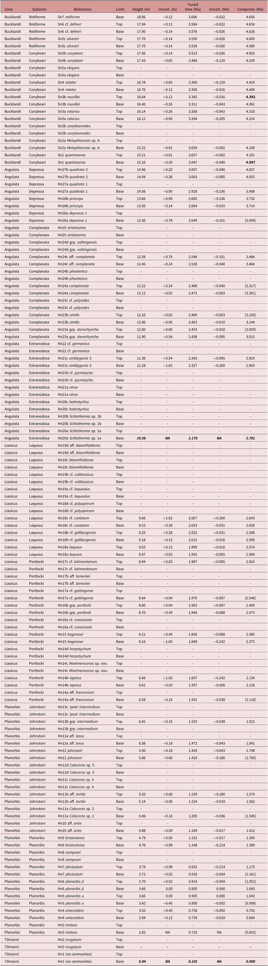
Square brackets in the composite time column indicate that the value is influenced by the presence of an inferred hiatus. Bold numbers in the composite time column indicate reference levels. The base of the tuned time scale is the base of the Blue Lias Formation, whereas the base of the composite time scale is the inferred base of the Tilmanni Zone. The data for the base of the Tilmanni Zone and the base of the Angulata Zone are shown using bold italics as these levels are determined by correlation with West Somerset on the composite time scale (Section 9). Missing values (dashes) are indicated where a biohorizon boundary or limit has not been located precisely in the field. Uncert. – maximum uncertainty in biohorizon level; NA – not applicable.
Heights, tuned times and composite times for biohorizons at Lavernock, South Glamorgan
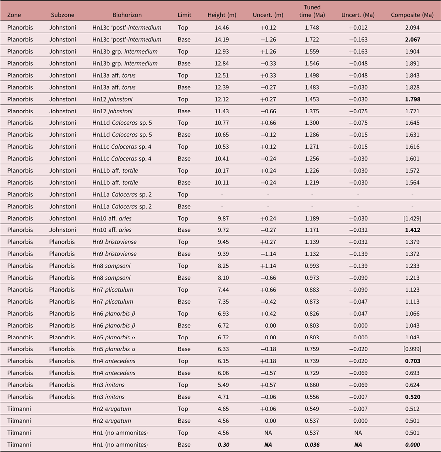
Square brackets in the composite time column indicate that the value is influenced by the presence of an inferred hiatus. Bold numbers in the composite time column indicate reference levels. The base of the tuned time scale is the base of the Blue Lias Formation, whereas the base of the composite time scale is the inferred base of the Tilmanni Zone. The data for the base of the Tilmanni Zone are shown using bold italics as these levels are determined by correlation with West Somerset on the composite time scale (Section 9). Missing values (dashes) are indicated where a biohorizon boundary has not been located precisely in the field. Uncert. – maximum uncertainty in biohorizon level; NA – not applicable.
In the Tilmanni and Planorbis zones, where the scale of the longest cycles is within a factor of two between Lyme Regis (0.46 m; Fig. 6) versus West Somerset and Lavernock (0.81 m and 0.70 m, respectively; Figs 6, 7), the cyclicity is encoded in a similar fashion at all the sites (Fig. 8). The longest wavelength cycles in vol. MS (i.e. inverse of calcium carbonate content) are usually associated with bundles or groups of a few (up to four) closely spaced limestones separated by beds of marls and/or laminated shale. This relationship changes on the West Somerset Coast in the Liasicus and Angulata zones where the bundles of limestones are more variable, but commonly the limestones are more numerous and the intervening marl and laminated shale beds can represent a far greater proportion by thickness of the whole cycle (Figs 9, 10). Additionally, in some cases, isolated limestone beds occur in the maxima in vol. MS (minima in carbonate contents) in the longest cycles in West Somerset.
These observations can be understood by focusing in more detail on the data from the Planorbis Zone at Lavernock and Lyme Regis (Fig. 11a) and on an interval including the Angulata–Bucklandi zonal boundary in West Somerset (i.e. the base Sinemurian GSSP) and Lyme Regis (Fig. 11b). The upper interval includes some of the clearest spectral evidence for regular cyclicity at these localities (West Somerset section D, Lyme Regis section C; Figs 6, 7).
(a) Data and band-pass filter outputs from the Planorbis Zones at Lavernock and Lyme Regis. The columns to the left of the vol. MS data have the same indication of lithologies as Figures 4 and 5. Band-pass filter outputs have been labelled with the inferred orbital cycles: E – eccentricity; O – obliquity; P – precession; B – base; T – top.

(Continued) (b) Data and band-pass filter outputs from around the Angulata–Bucklandi zonal boundary from the West Somerset Coast and Lyme Regis. GSSP – Global Boundary Stratotype Section and Point (base of the Sinemurian Stage).
In addition to the filter output of the longest cycles, band-pass filtering in the depth domain has been used to isolate the cycles inferred to represent obliquity and precession forcing. The filter outputs are summed and combined with the means and shown on the right for each site (Fig. 11a, b). Summing the filter outputs, representing the three scales of regular cycles in the depth domain, provides a good approximation of the original vol. MS time series. Note that minor mis-matches between the original time series and the summed data remain because the variability from very low frequencies and from very high frequencies is excluded from the filter outputs.
At Lyme Regis, the expression of the longest cycles in the Angulata and Bucklandi zones (Fig. 11b) is very similar to that observed in the Planorbis Zone (Fig. 11a). The long-wavelength minima in vol. MS (maxima in carbonate contents) at Lyme Regis are associated with one, two or three closely spaced limestone beds. The shorter wavelength cycles (inferred periods of 36.6 ka and ∼20 ka), indicated by O and P in Figure 11b for Lyme Regis, account for subdivisions of individual limestone beds and for variations in vol. MS over intervals of centimetres within the marls and shales, as shown by the variations in high-resolution %CaCO3 and %TOC data for Lyme Regis beds 13 to 23 in figure 2 of Weedon et al. (Reference Weedon, Jenkyns and Page2018).
In West Somerset, in the Tilmanni and Planorbis zones, the limestone beds are closely spaced and nearly always occur at the minima of vol. MS (maximum carbonate) in the eccentricity cycles (Fig. 8). By contrast, around the level of the Angulata–Bucklandi zonal boundary, the limestone beds are less closely spaced and are not restricted to the minima in vol. MS of the long-wavelength cycles (Fig. 11b). Some limestone beds are associated with the vol. MS minima of the inferred obliquity and precession cycles that occur at the maxima in vol. MS of the inferred eccentricity cycles. The contrast in limestone distribution in West Somerset in the Tilmanni and Planorbis zones with the distribution in the Liasicus and Angulata zones can be explained in terms of differences in average accumulation rates influencing the formation of limestone beds.
Limestone formation is believed to have been associated with astronomically driven variations in storminess and storm-related pauses in sedimentation that led to cementation within a zone of anaerobic methane oxidation that was a few tens of centimetres thick and close to the sediment–water interface (Weedon et al. Reference Weedon, Jenkyns and Page2018). In the Tilmanni and Planorbis zones in West Somerset and at Lavernock, and at Lyme Regis for the whole of the Hettangian, accumulation rates were sufficiently low that cementation starting at a particular level could continue within the zone of aerobic methane oxidation for considerable time. This process allowed single or groups of limestone beds to be formed within up to half an eccentricity cycle (50 ka), occasionally producing limestone beds ‘welded’ together (e.g. beds H26 to H28; bed 19, 23; and beds 25 to 27 at Lyme Regis). By contrast, in West Somerset, when accumulation rates were much higher in the Angulata and Bucklandi zones, cementation at a particular level apparently could not be maintained for more than half an obliquity cycle (∼18 ka) before burial below the level of limestone growth. This limitation caused limestone beds to be formed at much wider spacing and their spacing to be determined primarily by the obliquity and precession cycles rather than the short eccentricity cycles.
Hence, when accumulation rates at West Somerset were around a factor of two greater than Lyme Regis in the Tilmanni and Planorbis zones, individual limestone beds can potentially be correlated between the two sites. However, owing to substantially increased rates of accumulation at West Somerset in the Liasicus, Angulata and Bucklandi zones, individual limestone beds at Lyme Regis commonly equate to groups of limestones at West Somerset (cf. Hallam, Reference Hallam1964, Reference Hallam1986, Reference Hallam1987; Weedon, Reference Weedon1987).
7. Biohorizons and time
Each stratigraphic interval associated with an ammonite biohorizon conceptually corresponds to the total chronological range of a single named taxon, as definable by the observed morphological variation of a reference assemblage. The expression of a biohorizon in the geological record may correspond to a preservational ‘window’ that represents a proportion of the total chronological interval (Page, Reference Page2017). The intervals between biostratigraphic ‘events’, during which evolutionary changes affecting hard-part morphology can occur, facilitate the recognition of distinct index species in different biohorizons. Accordingly, biohorizonal schemes, such as that for the Hettangian–Sinemurian sequences of the Blue Lias Formation, provide discrete, non-overlapping correlative units, typically with stratigraphic intervals between biohorizons (Page, Reference Page, Lord and Davis2010 a, Reference Page2017).
Many authors such as Buckman (Reference Buckman1902), Shaw (Reference Shaw1964) and Callomon (1988) have argued that biostratigraphic boundaries can be regarded as time lines, especially by comparison with lithostratigraphic boundaries, with the exception of event beds such as volcanic ash layers/bentonites and meteoritic fallout. Living Nautilus is known to travel up to 150 km laterally in a year (Saunders & Spinoza, Reference Saunders and Spinoza1979). Page (Reference Page2017) calculated that even simply floating (planktonic) organisms could potentially circumnavigate the globe equatorially in just 2.56 years in the absence of land barriers. The planktonic larval stage and adult nektonic life style of ammonites meant there was the potential for new evolution-derived traits, or even new species, to spread rapidly over large distances. Hence, ammonite biohorizonal boundaries, at least on a local scale, can potentially be considered to be time lines. Nevertheless, the main issue in terms of time-scale construction is how accurately the biostratigraphic boundaries have been identified within the lithostratigraphic sections.
There are a variety of ways that ammonites were preserved in the Blue Lias Formation such that specifically determinable ammonite faunas can be recovered from all the different lithofacies (Paul et al. Reference Paul, Allison and Brett2008; Weedon et al. Reference Weedon, Jenkyns and Page2018). Aside from very rare concealment of intervals of less than 0.4 m thickness by modern beach sediments, continuous, systematic sampling by breaking up bedrock, analogous to breaking up borehole cores with a cross-sectional diameter of 0.3 m, supplemented by sampling from limestone surfaces sometimes tens of square metres in extent on wave-cut platforms, was achieved mainly between 2012 and 2016 on the West Somerset Coast, Lyme Regis and at Lavernock. At levels where ammonites were detected by the systematic sampling in the marls or shales, more material was examined to recover sufficient specimens for reliable taxonomic determination. The more detailed sampling typically involved packages of 0.1 m in vertical thickness or from intervals of a few centimetres to 0.3 m, representing the full vertical persistence of a characteristic fauna.
The sampling resulted in recovery of ammonite specimens from 102 levels from the base of Hn2 to the base of Sn1 on the West Somerset Coast, or an average sample spacing of 0.71 m. Similarly, 26 levels were recorded from the base of Hn4 to the base of Sn1 at Lyme Regis. Allowing for an interval lacking identifiable ammonites between 9.66 m and 11.06m, the average spacing is 0.41 m. Finally, at Lavernock, 34 levels yielded ammonite specimens between the base of Hn2 and the top of Hn14a, producing an average spacing of 0.30 m. In total, more than 3500 specifically identifiable specimens were collected and the results combined with examination of W. D. Lang’s collections from the Lyme Regis area in the Natural History Museum, London (including specimens figured by Page, Reference Page, Lord and Davis2010 a).
The positions of the biohorizon boundaries that can be reliably recognized from specimens of characteristic faunas rather than just from isolated fragments are provided to the nearest centimetre in Tables 1–3. Figure 11a, b plots both the tops and bases of biohorizons where located. In general, it is apparent from this figure that the individual biohorizon intervals occupy a small proportion of the longest wavelength cycles, i.e. representing less than 100 ka.
Both the relative thickness of strata and the numbers of the longest cycles present between specific biohorizons differ between localities (Figs 8–10). For example, in the Planorbis Subzone, the interval from the base of biohorizon Hn5 to the base of biohorizon Hn6 involves a greater thickness and more long-wavelength cycles in West Somerset compared to both Lavernock and Lyme Regis, even when allowing for the uncertainty in biohorizon limits indicated by vertical error bars (Fig. 8). Similarly, in the Johnstoni Subzone, there are more strata and more long-wavelength cycles from the top of Hn12 to the base of Hn14a at Lavernock than elsewhere (Fig. 8).
At other levels, even though overall the West Somerset sequence is far thicker than that at Lyme Regis, allowing for the uncertainties in biohorizon boundary positions, there are intervals that are anomalously thin. For example, in the Conybeari Subzone from the base of Sn2a to the top of Sn3b (Figs 10, 11b) the West Somerset interval is anomalously thin compared to Lyme Regis and has fewer long-wavelength cycles. If the biohorizon boundaries as located in the Blue Lias Formation can be treated as reliable approximations to time lines, then the anomalously reduced relative thicknesses combined with the reduced numbers of inferred 100 ka cycles between common biohorizon levels can be explained in terms of local stratigraphic gaps or sedimentologically condensed intervals. Weedon et al. (Reference Weedon, Jenkyns and Page2018) discussed the field evidence for such gaps.
8. Tuned time scales
8.a. Power spectra of the tuned data
It is now clear that tuning time series to an orbital solution can result in considerable distortions that bias the resulting power spectra (e.g. Huybers & Wunsch, Reference Huybers and Wunsch2004; Proistosescu et al. Reference Proistosescu, Huybers and Maloof2012). Even with good constraints on the overall time scale, careful processing is needed when tuning data to an orbital solution (Huybers & Aharonson, Reference Huybers and Aharonson2010; Meyers, Reference Meyers2015; Zeeden et al. Reference Zeeden, Meyers, Lourens and Hilgen2015). Here, the tuning has been conducted without reference to an orbital solution by assuming naively that the longest cycles shown as filter outputs in Figures 8–10 relate to a fixed-period (100 ka) short cycle in eccentricity forcing. Local tuned time scales have been constructed by simply fixing successive filter output vol. MS minima (carbonate maxima) at 100 ka intervals; the associated power spectra are shown in Figure 12. For each location, the start of the tuned time scale is fixed at the base of the Blue Lias Formation. Tables 1–3 list the implied tuned time-scale positions of the biohorizon boundaries and their uncertainties at West Somerset, Lyme Regis and Lavernock. Biohorizonal boundaries have not been identified in detail yet at Southam Quarry.
Power spectra of the whole of the tuned vol. MS time series for each locality. FDR – false discovery rate level; CL – confidence level; Backgnd – spectral background; E – eccentricity; O – obliquity; P – precession; MCCL – Monte Carlo confidence level; ka – thousand years.

Not surprisingly, at the frequency of the 100 ka tuning, the power spectra of the tuned data have spectral peaks exceeding the 1 % FDR (Fig. 12). Encouragingly, the spectra also have concentrations of power at or above the 99 % level for the Early Jurassic precession periods at all locations apart from Southam Quarry and above the 99 % level for obliquity at Somerset and Lyme Regis.
Significant spectral peaks occur near the frequency of Early Jurassic obliquity (i.e. 1/36.6 ka) on the West Somerset Coast at 1/50 and 1/29 ka, and at 1/43 ka at Lavernock. Similarly, spectral peaks occurring near the frequencies of Early Jurassic precession (1/21.5 and 1/18.0 ka) occur at 1/14 ka at Lyme Regis and at 1/16 ka at Lavernock. The 1/50 ka peak at West Somerset might represent a harmonic related to non-sinusoidal variations at the 100 ka scale. However, the other peaks near the obliquity and precession frequencies cannot be explained numerically as being due to either harmonics or combination tones. Instead, they most likely indicate that the tuning using 100 ka tie levels has failed to remove shorter term variations in accumulation rates and/or result from using an unrealistic perfectly fixed 100 ka period for the short eccentricity cycles.
The filter outputs of Figure 11 in the depth domain show modest variations in wavelengths of the inferred obliquity- and precession-related cycles. The differences in frequencies between the nearby peaks and the expected frequencies imply variations in accumulation rate within the 100 ka cycles of 15 to 30 % (e.g. 1/43 ka versus 1/36.6 ka; 1/14 ka versus 1/18 ka). Higher resolution tuning has not been attempted, since the strongest evidence for regular cyclicity in the depth domain resides with the longest wavelength regular cycles. Higher resolution tuning would not substantially modify the overall tuned time scales.
The spectral peaks related to tuning were tested against a null model as advocated by Proistosescu et al. (Reference Proistosescu, Huybers and Maloof2012), implemented as described in Section 3.f. In every case, the tuning at the frequency of the short eccentricity cycle exceeds the 99 % MCCL shown using dashed horizontal lines in Figure 12. At the frequency range of precession cycles, the 99 % MCCL is exceeded at Lyme Regis and at Lavernock. At the scale of obliquity cycles, the 95 % MCCL is exceeded at West Somerset and Lyme Regis. These results suggest that tuning of the longest regular cycles to the 100 ka eccentricity period is credible and useful, i.e. the increase in regularity is greater than that expected from tuning random numbers.
8.b. Shaw plots of tuned data
Graphic correlation of the positions of the biohorizon boundaries on the tuned time scales at West Somerset, Lyme Regis and Lavernock is explored in Figure 13. The figure includes the vertical and horizontal error bars associated with each Shaw plot tie-point as derived from the uncertainty in time estimates listed with the tuned time-scale ages in Tables 1–3. The tuning was intended to remove the effects of variations in sedimentation rates on the relative positions of the biohorizon boundaries at time scales longer than 100 ka. Therefore, unlike the Shaw plot of biohorizons using stratigraphic heights (fig. 8 of Weedon et al. Reference Weedon, Jenkyns and Page2018), plots using tuned time should ideally have lines of correlation that slope at 45° (the ‘1:1 line’), indicating the same time intervals between biohorizon boundaries at pairs of localities.
(a–c) Shaw plots based on the positions of the biohorizon boundaries on the tuned time scales relative to the local base of the Blue Lias Formation: (a) Lyme Regis versus West Somerset; (b) Lavernock versus Lyme Regis; (c) Lavernock versus West Somerset. Note that for each location the base of the tuned time scale is the base of the Blue Lias Formation (i.e. within the uppermost Rhaetian, Triassic). In (a) and (c) the vertical arrows emerging from the West Somerset axis and projected horizontally onto the Lyme Regis axis show the implied positions of the base of the Tilmanni Zone and the base of the Angulata Zone according to the composite time scale (Section 9.b). The uncertainty in the positions of the biohorizon limits (i.e. tops and bases) is indicated using grey vertical and horizontal bars associated with each plotted point. (d–f) Shaw plots based on the positions of the biohorizon boundaries on the composite time scale relative to the base or inferred base of the Jurassic (base of the Hettangian Stage): (d) Lyme Regis versus West Somerset; (e) Lavernock versus Lyme Regis; (f) Lavernock versus West Somerset. The base of the composite time scale is the base of the Jurassic (base of Hn1). The vertical long grey arrow emerging from the West Somerset axis and projected horizontally to the Lyme Regis axis indicates the inferred location of the base of the Angulata Zone. The uncertainty in the positions of the ‘independent’ biohorizon limits are indicated using black vertical and horizontal bars. All plotted data are listed in Tables 1–3. Ma – million years. Abbreviations for subzones: Plan. – Planorbis; John. – Johnstoni; Port. and P – Portlocki; L. – Laqueus; Ext. and Ex. – Extranodosa; Depr. and Dep. – Depressa; Conyb. and Cony. – Conybeari. Abbreviations for zones: Tilman – Tilmanni; Lias, L – Liasicus; Buckl. – Bucklandi.

In practice, the hiatuses inferred by Weedon et al. (Reference Weedon, Jenkyns and Page2018) contribute to significant deviations from the ideal line of correlation (shown as sloping grey dashed lines in Fig. 13a, b, c). Note that despite the uncertainty in the biohorizon limits, in most cases the line of correlation is tightly constrained to step-like deviations that correspond to the hiatuses discussed by Weedon et al. (Reference Weedon, Jenkyns and Page2018). On the other hand, the hiatus indicated at the base of Hn12 for Lyme Regis in Figure 13a, b, and at the base of Hn14a for Lyme Regis in Figure 13a, might result from biostratigraphic uncertainty. Despite the stratigraphic gaps, there is a noticeable tendency for the lines of correlation to repeatedly run parallel to the ideal line of correlation. This result indicates that, in the long term, these tuned sections agree fairly closely in terms of the amount of elapsed time and that the longest wavelength regular cycles at Lavernock, West Somerset and Lyme Regis have been correctly associated with the same forcing period (inferred to relate to short eccentricity cycles).
8.c. Minimum durations from the tuned time scale
Allowing for the possibility of undetected gaps, the tuned time scales provide estimates for the minimum time represented by the ammonite biohorizons. Sixty-two biohorizons are listed in Table 4 (Page, Reference Page, Lord and Davis2010a; Weedon et al. Reference Weedon, Jenkyns and Page2018) with, dependent on whether both the base and top of a biohorizon has been located in the field, minimum durations available from two sites in 25 cases and from three sites in six cases. The largest minimum duration calculated in each case is indicated in bold in Table 4.
Minimum ammonite biohorizon durations in ka based on time scales derived from tuning of the Blue Lias Formation using presumed short eccentricity cycles

Duration estimates are only available where both the top and base have been located (as listed in table 1 of Weedon et al. Reference Weedon, Jenkyns and Page2018). The largest minimum duration for each biohorizon is indicated in bold.
The range of the largest minimum durations for the biohorizons is 0.7 ka to 276 ka, averaging 19.4 ka (Table 4). Since the tuning is based on cycle boundaries at the 100 ka spacing, individual estimates of minimum durations much less than this should not be regarded as necessarily very precise. Nevertheless, considering all 62 biohorizons together, a clear pattern emerges: 58, or ∼94 %, of the largest minimum estimates across the sites are less than 41 ka and nine of these, or ∼15 % of the total, are less than 3 ka. This result is critical since it implies that the time intervals associated with ammonite biohorizons in the Hettangian of Britain represent small proportions of the 100 ka cycles in nearly every case. It also confirms the conclusion of Buckman (Reference Buckman1902) that different biohorizons (‘hemera’ in his terminology) are likely to represent a variety of durations (Page, Reference Page2017).
Tables 1–3 for the West Somerset Coast, Lavernock and Lyme Regis, also allow estimates of the minimum time between the base of one biohorizon and the next (i.e. the biohorizon plus the succeeding interval; see Page, Reference Page2017). Minimum durations are available for two sites in 21 cases and for three sites in two cases. The largest minimum durations from biohorizon base to the next biohorizon base ranges from 6.2 ka to 276 ka and averages 63.9 ka, with 42 % of estimates less than 41 ka, and 77 % less than 100 ka.
The uncertain location of the base of the Tilmanni Zone (base of Hn1) at Lyme Regis is discussed later (Section 9.b), but it is helpful to compare long comparable intervals of tuned data between West Somerset and Lyme Regis. The minimum amount of time implied by the West Somerset Coast tuned time scale between the base of the Rotiforme Subzone (base Sn5c at 3.793 Ma) and the base of the Planorbis Zone (base Hn3 at 0.808 Ma) is 2.985 Ma (Table 1). This figure differs by just 6 % from the results for Lyme Regis for the same interval: 3.539 Ma minus 0.710 Ma, or 2.829 Ma (Table 2). Since the tuning exercise adjusts for differences in sedimentation rates, but not for hiatuses, the agreement on elapsed time over the long term is indicative of surprisingly similar overall completeness at these two sites.
In terms of estimating the minimum duration of the Hettangian Stage, but in the absence of the correlating ammonite fauna in Britain, the base of the Jurassic (base Hn1) has been estimated in the West Somerset section as ∼1.5 m above the base of the Blue Lias Formation using δ13Corg data (Clémence et al. Reference Clémence, Bartolini, Gardin, Paris, Beaumont and Page2010; Hillebrandt et al. Reference Hillebrandt, Krystyn, Kürschner, Bonis, Ruhl, Richoz, Schobben, Ulrichs, Bown, Kment, McRoberts, Simms and Tomãsových2013). On the West Somerset tuned time scale, the base of Hn1 occurs at 0.280 Ma and the base of Sn1 at 3.508 Ma, so the minimum duration for the Hettangian is ∼3.23 Ma (Table 1). The base of Hn1 was estimated previously at ∼0.60 m above the base of the Blue Lias at Lyme Regis (Weedon et al. Reference Weedon, Jenkyns and Page2018). However, we delay providing an estimate of the duration of the Hettangian Stage from the tuned time scale at Lyme Regis until after reconsideration of the position of the base of the Jurassic in this locality (Section 9.b).
9. Composite time scale
9.a. Construction of the composite time scale
The scaling of the tuned time scales depends only on the location of the boundaries of the long sedimentary cycles of Figures 8–10 and not on the biostratigraphic data. It was shown in Section 8.c that 94 % of the biohorizons in the Hettangian and basal Sinemurian of southern Britain have minimum interval durations from the local tuning of less than 41 ka. By using 100 ka cycles to constrain sedimentation rates, very short-term changes in sedimentation rate cannot be resolved. Weedon et al. (Reference Weedon, Jenkyns and Page2018) argued that the formation of limestones preserving ammonites was associated with rapid deposition in storms followed by storm-related pauses in accumulation and/or erosion with the intensity and/or frequency of storms under orbital-climatic control. Consequently, it is conceivable that some biohorizons constrained here to less than a few ka actually represent very short time intervals (perhaps less than 1 ka), in some cases perhaps related to particular conditions of preservation (Page, Reference Page2017). Nevertheless, the errors in stratigraphic heights typically translate into relatively small errors on the tuned time scales, as shown by the majority of error bars in Figure 13a, b, c (Tables 1–3).
Accordingly, as an exercise, we have assumed that the biohorizon limits as currently known can be regarded as providing reliable approximations to time lines. By combining the tuned time scales with the biostratigraphic data, a ‘composite time scale’ was constructed for Lavernock, the West Somerset Coast and Lyme Regis. This procedure is analogous to the estimate of the duration of the Oligocene based on combining cyclostratigraphic and biostratigraphic data from four sites on the Ceara Rise, western equatorial Atlantic (Weedon et al. Reference Weedon, Shackleton and Pearson1997), but with an added allowance for hiatuses.
Hiatuses have been located using the steps in the Shaw plots where anomalously short intervals of tuned time occur relative to another section (Fig. 13a, b, c). They have been indicated on the composite time scale as occurring immediately below the base of biohorizons or immediately above the top of biohorizons (Figs 14, 15). Constrained by the biostratigraphic data, this method does not allow identification of very short intervals of missing record (e.g. corresponding to <50 ka). Furthermore, the distribution of hiatuses between the biostratigraphic controls is not known; between some biohorizon limits there might be many small intervals of time not represented by sediment rather than the single gaps shown. As noted in Section 8.b, the steps in the Shaw plots associated with the inferred hiatuses at Lyme Regis indicated at the base of Hn12 and Hn14a in Figure 13a, b could be eliminated by slight adjustment of the tie-points, given the comparatively large biostratigraphic uncertainty bars. Nevertheless, the composite time scale would be only minimally affected if these specific hiatuses were treated as illusory (Fig. 14).
Data from Lavernock, the West Somerset Coast and Lyme Regis shown on the Tilmanni and Planorbis zone interval of the composite time scale. The locations of the stratigraphic gaps were established using Figure 13a, b, c. Biohorizon boundaries that are located ‘independently’ are shown in grey. Biohorizon levels fixed by reference to another locality are shown in black. Biohorizon boundary levels used to define a composite time are shown in black with an arrow pointing to the referred locality. Biohorizon boundaries believed to occur at hiatuses (listed in square brackets in Tables 1–3) are not shown. At Lavernock and Lyme Regis, the dashed lines indicating the base of the Tilmanni Zone (based Hn1) are labelled ‘C’ since they were established by correlation on the composite time scale with the West Somerset Coast (Section 9.b). The columns to the left of the vol. MS data indicate the following lithologies: white – light marl or homogeneous limestone; grey – dark marl; black – laminated shale or laminated limestone. ‘E’ above the filter output columns indicates inferred short eccentricity cycles. Ma – million years; Lias. – Liasicus; Port. – Portlocki; Bed no. – bed number; DkM/Lam. – dark marl, laminated shale or laminated limestone; B – base; T – top.

Data from the West Somerset Coast and Lyme Regis shown on the Liasicus and Angulata zone and Conybeari Subzone interval of the composite time scale. Left: data from Southam Quarry on the local tuned time scale aligned to match the composite time scale at the base of the Bucklandi Zone. The locations of the stratigraphic gaps were established using Figure 13a. At Lyme Regis, the dashed line indicating the base of the Angulata Zone (based Hn20a) is labelled ‘C’ since it was established by correlation on the composite time scale with the West Somerset Coast (Section 9.b). The composite time of Top Hn14a at West Somerset was fixed by the reference time at Lavernock (Fig. 14). Biohorizon boundaries that are located ‘independently’ are shown in grey. Biohorizon levels fixed by reference to another locality are shown in black. Biohorizon boundary levels used to define a composite time are shown in black with an arrow pointing to the referred locality. Biohorizon boundaries believed to occur at hiatuses (listed in square brackets in Tables 1–3) are not shown. Within the bed number column for Lyme Regis, the grey arrow labelled ‘IC’ indicates the level of the intraclast in bed 25 described by Weedon et al. (Reference Weedon, Jenkyns and Page2018). The columns to the left of the vol. MS data indicate the following lithologies: white – light marl or homogeneous limestone; grey – dark marl; black – laminated shale or laminated limestone. ‘E’ above the filter output columns indicates inferred short eccentricity cycles. Ma – million years; P – Planorbis; J – Johnstoni; Laq. – Laqueus; Extran. – Extranodosa; Bed no. – bed number; DkM/Lam. – dark marl, laminated shale or laminated limestone; B – base; T – top.

In some cases, the indication of unrecorded time could result from an interval of condensation below the resolution of the method due, for example, to sediment starvation during maximum flooding, rather than due to storm-related erosion. Possible examples of gaps on the composite time scale due to unresolved condensation could be located near the top of the Portlocki Subzone at Lyme Regis and near the base of the Laqueus Subzone at West Somerset (Fig. 15). The time of the Portlocki–Laqueus subzonal boundary, near the middle of the Liasicus Zone, is likely to have been a period of maximum flooding during rising sea level, and hence potentially associated with condensation offshore (Hesselbo, Reference Hesselbo2008; Weedon et al. Reference Weedon, Jenkyns and Page2018).
Unlike the tuned time scales, which reference the local bases of the Blue Lias Formation, the base of the composite time scale is taken as the base of the Hettangian (base of Hn1). Segments of data between the inferred gaps represent the amount of time determined on the tuned time scales. Individual segments of tuned data have been located on the composite time scale by adopting a single reference composite time, as previously determined at another site, for a single biohorizon level (a ‘reference level’) within each segment, provided that it does not occur at the level of an inferred hiatus at either the definition site or at the correlation site. Reference levels are listed for the composite time scale in normal bold text in Tables 1–3.
The positions of the biohorizons on the composite time scale are listed in the last columns of Tables 1–3. In the tables, where a biohorizon boundary is inferred from Figure 13a, b, c to occur at a hiatus, the composite time is indicated in square brackets. We indicate how each local biohorizon top or base that does not occur at an inferred hiatus was located on the composite time scale in Figures 14 and 15 using three methods. Biohorizon limits treated as reference levels are shown as horizontal black lines, plus arrows pointing to the site or sites where the level of a segment of data has been fixed. Within each data segment there is one biohorizon top or base, shown as a horizontal black line, that is fixed using a reference level defined elsewhere. Horizontal grey lines in Figures 14 and 15 show the biohorizon limits within a segment of data that are spaced according to the local tuned time scale relative to the fixed level. Such levels are described here as ‘independent’ tie levels since they are not fixed at the reference levels. Note that the use of the reference levels means that the composite time scale has been constructed without requiring consistency in the relative phase (e.g. maxima or minima) of the inferred short eccentricity cycles between sites.
In addition to the hiatuses previously discussed by Weedon et al. (Reference Weedon, Jenkyns and Page2018), the composite time scale implies the presence of a hiatus at or very close to the Planorbis–Liasicus boundary on the West Somerset Coast, where there is an abrupt change in the average vol. MS of the non-limestone lithologies (Figs 5, 14). A stratigraphic gap at this level in this site had previously been inferred from comparison of gamma-ray logs (Bessa & Hesselbo, Reference Bessa and Hesselbo1997).
Figure 15 indicates a stratigraphic gap on the West Somerset Coast within the lower part of the Laqueus Subzone, Liasicus Zone, despite the absence of sedimentological, trace-fossil or body-fossil evidence of a gap within the associated black, laminated shales. Nevertheless, in April 2018 after initial submission of this paper, KNP observed a previously unknown interval of strata between biohorizons Hn18a and Hn18b including a limestone bed located in a previously obscured part of the foreshore at Quantocks Head, West Somerset. This location is close to an undescribed growth fault that was active during deposition of the Hettangian–Lower Sinemurian strata (Jenkyns & Senior, Reference Jenkyns and Senior1991). The new observation supports the presence of a stratigraphic gap in the section that was originally logged. The limestone bed at Quantocks Head corresponds to the limestone bed H70 at Lyme Regis. Indeed, the differences in relative thicknesses between the base of Hn18a and the top of Hn18b at these sites shown in Figure 9 could have been used to predict the possibility of missing strata on the West Somerset Coast.
Similarly, despite the lack of field evidence within laminated shales, we are confident that the significant hiatus inferred in the Planorbis Subzone, Planorbis Zone, at Lavernock just below bed 38 of Waters & Lawrence (Reference Waters and Lawrence1987) is genuine, considering the small uncertainty in the associated biohorizon limits (Figs 8, 13c).
At Lyme Regis in bed 25 in the Conybeari Subzone, Bucklandi Zone, the presence of a bored and encrusted limestone intraclast proves that some strata have been removed (Weedon et al. Reference Weedon, Jenkyns and Page2018). However, the presence of a gap below the base of Sn3b at West Somerset precludes indication of a gap on the composite time scale corresponding to bed 25 and the top of Sn3b at Lyme Regis (Fig. 15). Given the near coincidence in time of the hiatus preceding the base of Sn3b at West Somerset with the Lyme Regis data that includes missing strata in bed 25 (indicated by the ‘IC’ and a grey arrow in Fig. 15), the composite time scale certainly underestimates the duration of the Conybeari Subzone. A longer Conybeari Subzone than indicated in Figure 15 is consistent with the uncertainty in the position of the top of this subzone at Southam Quarry.
9.b. The base of the Tilmanni and Angulata zones at Lavernock and Lyme Regis
The position of the base of the Tilmanni Zone has been re-estimated at Lavernock and Lyme Regis, by correlation with the West Somerset section on the composite time scale, and hence differs from the levels inferred by Weedon et al. (Reference Weedon, Jenkyns and Page2018). The new estimates use the data below the base of Hn3 (base of Planorbis Zone) at each site on the composite time scale with the assumption that there are no gaps present in the Tilmanni Zone (Fig. 14). Given the lack of biostratigraphic data, this methodology provides a possible solution to the problem of locating the base of the Jurassic System at these sites. The composite time-scale correlations suggest that the base of the Jurassic can be revised at Lyme Regis from 0.60 m above the base of the formation previously (Weedon et al. Reference Weedon, Jenkyns and Page2018) to a figure of 0.84 m (Table 2). Similarly, this level at Lavernock has been revised from our earlier estimate of 1.86 m to 0.30 m above the base of the formation (Table 3).
Compared to the level indicated by Weedon et al. (Reference Weedon, Jenkyns and Page2018), the new estimated base of the Tilmanni Zone at Lavernock is closer to the upper maximum in δ13Ccarb of Korte et al. (Reference Korte, Hesselbo, Jenkyns, Rickaby and Spotl2009), which Clémence et al. (Reference Clémence, Bartolini, Gardin, Paris, Beaumont and Page2010) showed occurs close to the inferred level of the base Jurassic on the West Somerset Coast. Visually, the new estimates of the base of the Tilmanni Zone at Lyme Regis and Lavernock imply coincidences of similar variability of the vol. MS data in Figure 14. Independent constraints, perhaps from non-ammonite taxa such as nannofossils or other microfossils, are required to test the new estimates of the position of the base of the Tilmanni Zone at these two sites.
Based on incomplete ammonite records, the base of the Angulata Zone has been estimated to lie between 9.66 m and 11.06 m above the base of the Blue Lias Formation at Lyme Regis, while graphic correlation using stratigraphic heights indicates a level around 10.54 m (Weedon et al. Reference Weedon, Jenkyns and Page2018). The Shaw plot using the composite time scale in Figure 13d implies almost the same position at 10.56 m (i.e. within bed H77).
9.c. Shaw plot using the composite time scale
In many cases, on the composite time scale, a local biohorizon base or top is inferred to occur at a hiatus as located using the tuned time-scale data in Figure 13a, b, c. Consequently, the number of tie-points available in the Shaw plots for the composite time scale is reduced compared to the tuned time-scale plots (Fig. 13). Where the location of a biohorizon level has been fixed with reference to another section within a segment of strata between gaps (black lines without arrows in Figs 14, 15), the tie-point inevitably lies on the ideal line of correlation. Such tie-points are shown in grey in Figure 13d, e, f. On the other hand, where the position of a biohorizon level occurring between gaps has not been fixed with reference to another site (grey lines in Figs 14, 15), and is therefore considered to be somewhat ‘independent’, the corresponding tie-point is shown in black in Figure 13d, e, f with the associated uncertainty indicated by black error bars.
As seen in Figure 13d, e, f, the ‘independent’ tie-points define lines of correlation that closely approximate the ideal line of correlation. The differences between composite ages for the 26 independently located tie-points for West Somerset versus Lyme Regis range from +52 ka (for the top of Hn7 at Lyme Regis compared to the West Somerset Coast) to −32 ka with an average absolute (i.e. positive or negative) difference of 12 ka. This generally tight correspondence of the ‘independent’ tie-points to the ideal line provides support for the assumption that the biohorizon data provide relatively reliable time lines. Figures 14 and 15 provide expanded scales compared to the Shaw plots in Figure 13d, e, f and show the similarity of composite times of the independent biohorizon limits (horizontal grey lines) at the different sites.
An example of an independent tie-point lying notably off the ideal line of correlation in Figure 13d occurs near the base of the Portlocki Subzone, Liasicus Zone; this corresponds to the top of Hn14b. Figure 15 shows the anomalously large difference in times of the top of Hn14b at West Somerset and Lyme Regis compared to the good agreement of the estimated times of the base of Hn14a, the base and top of Hn15, and the base and top of Hn16b. The anomalous difference in composite time for the top of Hn14b could result from: (a) substantial error in locating the boundary in the field (e.g. too low at Lyme Regis indicated by the large vertical error bar); and/or (b) incorrect tuning of the basal Liasicus Zone at either location; and/or (c) an additional hiatus at Lyme Regis that cannot be resolved using the Shaw plot of Figure 13a.
9.d. Interval dating
Table 5 lists the minimum duration of the subzones, zones and stage according to the tuned time scales. Using the revised estimate of the base of the Tilmanni Zone (Section 9.b), the tuned time scale at Lyme Regis (Table 2) indicates a minimum duration for the Hettangian Stage of about ≥2.86 Ma, i.e. similar to the duration of ≥3.23 Ma from the tuned time scale for the West Somerset Coast (Section 8.c).
Minimum durations in Ma of the Hettangian Stage and the component ammonite subzones and zones according to the tuned time scale at each site
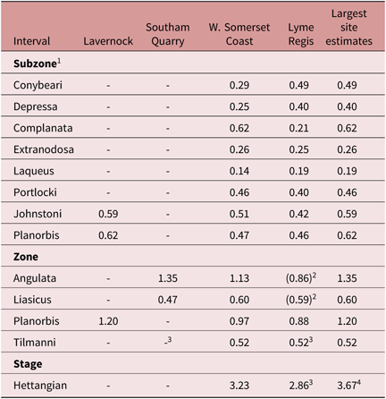
1 = Note there are no subzones within the Tilmanni Zone.
2 = Minimum duration of the Liasicus and Angulata zones at Lyme Regis based on correlation with the West Somerset Coast using the Shaw plot of Figure 13b.
3 = Base of the Tilmanni Zone at Lavernock and Lyme Regis located using the composite time scale (Section 9).
4 = The minimum duration of the Hettangian estimated here is based on the sum of the largest site estimates for each zone.
As explained in Section 1, normally cyclostratigraphic data at a single site would not be expected to produce definitive interval dating, given the likelihood of significant undetected stratigraphic gaps. An alternative way to estimate the duration of the Hettangian Stage from the tuned time scales is to consider the largest minimum duration estimates for each zone from the four localities studied. The results (Table 5) are ≥0.52 Ma for the Tilmanni Zone (West Somerset Coast); ≥1.20 Ma for the Planorbis Zone (Lavernock); ≥0.60 Ma for the Liasicus Zone (West Somerset Coast); and ≥1.35 Ma for the Angulata Zone (Southam Quarry). The total duration of the Hettangian Stage is, by this reckoning, ≥3.67 Ma, i.e. greater than the ≥2.86 and ≥3.23 Ma estimates from the single locality data of Lyme Regis and the West Somerset Coast. However, the composite time scale, by incorporating hiatuses (Section 9.a), implies that the minimum duration of the Hettangian was ≥4.10 Ma (Table 6), i.e. considerably longer than the estimates from the individual tuned time scales and somewhat longer than the estimate from pooling data from tuned time scales.
The minimum duration of the Hettangian Stage in Ma and the component ammonite subzones and zones according to the composite time scale for Lavernock, West Somerset Coast and Lyme Regis plus the estimated completeness at each site

The completeness, at the 10 ka scale, relates the minimum duration estimate from the tuned time scale of each site to the composite time scale.
1 = Base of Tilmanni Zone at Lyme Regis and Lavernock from correlation with West Somerset on the composite time scale (Section 9) assumes that there are no stratigraphic gaps.
The reliability of the composite time scale is limited by the availability of precisely located biohorizon limits. Several biohorizons have yet to be located at more than one site (Tables 1–3). Ultimately, the composite time scale needs to be tested by comparison with additional sites, ideally using radiometric dating constraints. Conversely, the current lack of biohorizon data at Southam Quarry means that this site is not part of the composite time scale. Data from this site do, however, provide an independent check on the minimum duration of the Angulata Zone according to the composite time scale.
The Southam Quarry data are plotted in Figure 15 using the tuned time scale, but with alignment with the composite time scale at the base of the Bucklandi Zone. The minimum duration implied from the tuned time scale there of ≥1.35 Ma (Table 5) is comparable, but slightly more than the ≥1.34 Ma according to the composite time scale (Table 6). Note that at Southam Quarry, minor incompleteness of the Angulata Zone is implied by (a) the presence of protrusive trace fossil Diplocraterion, indicative of minor erosion, in beds 19g, 23c and 23l (GP Weedon, unpub. D. Phil. Thesis, Univ. Oxford, 1987), and (b) by the bed-by-bed comparison with Rugby Quarry ∼14 km to the northeast described by Clements et al. (Reference Clements1977). There are ammonites present from at least as low as biohorizon Hn16 in the Portlocki Subzone, but the base of the Blue Lias Formation in Southam Quarry sits disconformably on the Upper Triassic Langport Member (Weedon et al. Reference Weedon, Jenkyns and Page2018). Hence, the Liasicus Zone is certainly far from complete there and, consequently, for this zone the corresponding tuned time scale interval is far shorter than that of the composite time scale (Fig. 15).
9.e. Stratigraphic completeness
The differences in interval durations according to the tuned time scales and the composite time scale allow calculation of local completeness. Table 6 indicates the local completeness, at the 10 ka scale (i.e. half a precession cycle), for the subzones, zones and stage. Table 5 permits calculation of local completeness at the 100 ka scale. Despite the large differences in average accumulation rates (Fig. 2), the overall completeness of the Hettangian Stage at Lyme Regis is not very different from that on the West Somerset Coast (69.8 % versus 78.8 %, respectively; Table 6).
Despite the similarity in overall completeness of these two localities, some shorter intervals are far less complete locally than others (Figs 14, 15). In the case of the Tilmanni Zone, in the absence of ammonite records, the correlation of the base of the zone from West Somerset to Lavernock and Lyme Regis assumed 100 % completeness (Section 9.b). In the Planorbis Zone, the only interval where three sites contribute to the composite time scale, Lavernock (75.5 %) appears to be more complete at the 10 ka scale than West Somerset (61.0 %) and Lyme Regis (55.3 %). The large gaps shown in the Angulata Zone at Lyme Regis (Fig. 15) probably explain for section B both the lack of significant Bayesian support for the presence of regular cyclicity (Fig. 6; Section 4.b) as well as the apparent mis-alignment of the 0.26 m spectral peak with the position of obliquity cycles (Fig. 6; Section 5.a).
9.f. Relative timing of laminated sediment deposition
The shortest duration intervals of laminated sediment deposition lasted less than 20 ka, with the pacing dictated by deposition of low-carbonate sediment (high vol. MS) as controlled by precession, obliquity and short eccentricity cycles, as seen for example in the Conybeari Subzone, Bucklandi Zone, of West Somerset and Lyme Regis (Figs 11b, 15). The longest duration intervals of continuous laminated sediment deposition lasted hundreds of thousands of years, for example in the Liasicus Zone of Southam Quarry (Fig. 15) and the Planorbis Subzone at Lavernock (Fig. 14).
The composite time scale allows comparison of the times when laminated shale was deposited in different sites. The conditions necessary for formation of individual laminated shale beds were apparently determined locally, but require further investigation to fully explain their occurrence. Consequently, individual beds cannot be confidently correlated between sites. Nevertheless, allowing for the incompleteness of the records, Lavernock, the West Somerset Coast and Lyme Regis have similar times with increased likelihood of deposition of laminated strata (a greater proportion of laminated shale or laminated limestone overall) late in the Planorbis Subzone and in the middle of the Johnstoni Subzone (Fig. 14). Similarities also exist in the timing of laminated shale deposition in the middle of the Portlocki Subzone, Liasicus Zone, at Lyme Regis and in West Somerset and possibly Southam Quarry, and in the Extranodosa Subzone and later part of the Depressa Subzone (Fig. 15).
Figure 16 shows all the vol. MS data plotted on the composite time scale together with the tuned Southam Quarry data, shown in grey, aligned using the base of the Bucklandi Zone (cf. Fig. 2). There is a lack of biohorizon controls for the Portlocki Subzone of the Liasicus Zone at both Lavernock and Southam Quarry. Nevertheless, the tuned time scales above the base of the Liasicus Zone at Lavernock, and below the top of the Liasicus Zone at Southam Quarry, imply that the maximum vol. MS of the marls and laminated shales occurred close to the time corresponding to the Portlocki–Laqueus subzone boundary as found in West Somerset and at Lyme Regis. The changes in likelihood of laminated sediment deposition and, separately, the changes in the vol. MS of the marls and laminated shales were nearly synchronous across the four sites (Fig. 16). The changes in average vol. MS were possibly linked to long-term (ammonite-zone scale) changes in sea level (Weedon et al. Reference Weedon, Jenkyns and Page2018).
Data from Lavernock, the West Somerset Coast and Lyme Regis on the complete composite time scale (compare with Fig. 2). Data from Southam Quarry in grey on the local tuned time scale have been aligned with the composite time scale using the base of the Bucklandi Zone for correlation. Dashed zonal boundaries have been located via correlations on the composite time scale (Section 9.b). ‘E’ above the filter output columns indicates inferred short eccentricity cycles. Ma – million years; Trias. – Triassic; Rha. – Rhaetian; Sinem. – Sinemurian; L. – Laqueus; Ext. – Extranodosa; Complan. – Complanata; Depr. – Depressa; Conyb. – Conybeari; GSSP – Global Boundary Stratotype Section and Point (base Sinemurian Stage).

10. The duration of the Hettangian Stage
Several estimates have been given (Section 9.d) for the duration of the Hettangian Stage: (a) ≥2.9 Ma from the tuned time scale for Lyme Regis and, separately, ≥3.2 Ma for the West Somerset Coast; (b) ≥3.7 Ma from the largest minimum tuned time-scale estimates for each zone based on all four sites (Lyme Regis, West Somerset Coast, Lavernock and Southam Quarry); and (c) ≥4.1 Ma from the composite time scale. Therefore, regardless of which estimate is used, the Hettangian Stage lasted far longer than the c. 2 Ma most recently inferred by others (Fig. 17; Schaltegger et al. Reference Schaltegger, Guex, Bartolini, Schoene and Ovtcharova2008; Ruhl et al. Reference Ruhl, Deenen, Abels, Bonis, Krijgsman and Kürschner2010; Guex et al. Reference Guex, Schoene, Bartolini, Spangenberg, Schaltegger, O’Dogherty, Taylor, Bucher and Atudorei2012; Ogg & Hinnov, Reference Ogg, Hinnov, Gradstein, Ogg, Schmitz and Ogg2012; Walker et al. Reference Walker, Geissman, Bowring and Babcock2013; Cohen et al. Reference Cohen, Finney, Gibbard and Fan2013; Ogg et al. Reference Ogg, Ogg, Gradstein, Ogg, Ogg and Gradstein2016). Note that the duration of the Hettangian indicated by Ogg & Hinnov (Reference Ogg, Hinnov, Gradstein, Ogg, Schmitz and Ogg2012) and Ogg et al. (Reference Ogg, Ogg, Gradstein, Ogg, Ogg and Gradstein2016) is derived directly from the cyclostratigraphic constraint of Ruhl et al. (Reference Ruhl, Deenen, Abels, Bonis, Krijgsman and Kürschner2010). Cohen et al. (Reference Cohen, Finney, Gibbard and Fan2013) took the boundary ages for the Hettangian directly from Ogg & Hinnov (Reference Ogg, Hinnov, Gradstein, Ogg, Schmitz and Ogg2012), while Walker et al. (Reference Walker, Geissman, Bowring and Babcock2013) simply rounded these ages to the nearest million years. However, the new cyclostratigraphic constraints are in better agreement with earlier, but fairly recent estimates of between 4.6 and 3.1 Ma (Pálfy et al. Reference Pálfy, Smith and Mortensen2000; Ogg, Reference Ogg, Gradstein, Ogg and Smith2004; Pálfy, Reference Pálfy2008; Walker & Geissman, Reference Walker and Geissman2009).
Estimates of the duration of the Hettangian Stage. Left: Geological time scales and direct dating publications indicate central estimates of between 4.6 and 1.96 Ma. Uncertainties in stage boundary ages are shown using vertical bars. Right: Constraints from cyclostratigraphy indicate a duration of the Hettangian Stage of ≥4.1 Ma. Sin. – Sinemurian.

High-precision dating of the base of the Jurassic (and base Hettangian Stage) from several regions has indicated a date close to 201.3 Ma before present (BP, Schaltegger et al. Reference Schaltegger, Guex, Bartolini, Schoene and Ovtcharova2008; Schoene et al. Reference Schoene, Guex, Bartolini, Schaltegger and Blackburn2010; Guex et al. Reference Guex, Schoene, Bartolini, Spangenberg, Schaltegger, O’Dogherty, Taylor, Bucher and Atudorei2012; Blackburn et al. Reference Blackburn, Olsen, Bowring, McLean, Kent, Puffer, McHone, Rasbury and Et-Touhami2013; Wotzlaw et al. Reference Wotzlaw, Guex, Bartolini, Gallet, Krystyn, McRoberts, Taylor, Schoene and Schaltegger2014). On the other hand, dating of the base of the Sinemurian Stage is far less certain.
The ∼201.3 Ma BP estimate for the base of the Hettangian Stage of Schaltegger et al. (Reference Schaltegger, Guex, Bartolini, Schoene and Ovtcharova2008), Schoene et al. (Reference Schoene, Guex, Bartolini, Schaltegger and Blackburn2010) and Guex et al. (Reference Guex, Schoene, Bartolini, Spangenberg, Schaltegger, O’Dogherty, Taylor, Bucher and Atudorei2012), revised by Wotzlaw et al. (Reference Wotzlaw, Guex, Bartolini, Gallet, Krystyn, McRoberts, Taylor, Schoene and Schaltegger2014), was based on U–Pb dating of zircon samples from ash beds in Peruvian sections, combined with just six levels yielding ammonites through what was inferred to be the whole of the Hettangian Stage. Inexplicably, however, the position of the base of the stage was placed just below the first occurrence of Psiloceras spelae (Hillebrandt & Krystyn), the indicator fossil of the basal Hettangian at the GSSP in Austria. Zircon sample LM4-185A was undoubtedly reworked since it is at least 2 million years older than expected given its stratigraphic position (Guex et al. Reference Guex, Schoene, Bartolini, Spangenberg, Schaltegger, O’Dogherty, Taylor, Bucher and Atudorei2012). This reworked sample was obtained just below sample LM4-19B, which was inferred to be from near the Hettangian–Sinemurian boundary (Schaltegger et al. Reference Schaltegger, Guex, Bartolini, Schoene and Ovtcharova2008; Guex et al. Reference Guex, Schoene, Bartolini, Spangenberg, Schaltegger, O’Dogherty, Taylor, Bucher and Atudorei2012). It is conceivable that sample LM4-19B also represents reworked material, and therefore the inferred upper limit of the Hettangian could actually be far younger than the 199.5 Ma BP calculated by Guex et al. (Reference Guex, Schoene, Bartolini, Spangenberg, Schaltegger, O’Dogherty, Taylor, Bucher and Atudorei2012).
The biostratigraphic placement of the top of the Hettangian–base Sinemurian in the same Peruvian sections is also problematic. The boundary was placed arbitrarily around half way between the highest identified Hettangian ammonites (Badouxia canadensis (Frebold)) and the first recorded ‘Sinemurian’ ammonite, identified as ‘Coroniceras’, representing a gap in ammonite records of 13 m (Schaltegger et al. Reference Schaltegger, Guex, Bartolini, Schoene and Ovtcharova2008). The latter ammonite was recorded around 11 m above the dated sample LM4-19B, although Guex et al. (Reference Guex, Schoene, Bartolini, Spangenberg, Schaltegger, O’Dogherty, Taylor, Bucher and Atudorei2012) showed the stage boundary occurring at the level of Badouxia canadensis (4 m below LM4-19B), despite the lack of ammonite recovery in the overlying 13 m of strata. Crucially, however, the alleged ‘Coroniceras’ and ‘Metophioceras’ specimens supposedly indicating the Sinemurian are completely unlike any European species of these genera and were recovered in the opposite stratigraphic order to that in which they might normally be expected to occur, with ‘Coroniceras’ recovered stratigraphically below ‘Metophioceras’ (e.g. Page, Reference Page, Lord and Davis2010 b). In reality, the close ribbed, non-tuberculated whorl fragments (fig. 4a, c of Schaltegger et al. Reference Schaltegger, Guex, Bartolini, Schoene and Ovtcharova2008) show strong affinities to Paracaloceras. This is a Late Hettangian arietitid genus known primarily from Mediterranean and Athabaskan/Andean province areas (sensu Page, Reference Page2008). Comparable specimens are illustrated by Longridge et al. (Reference Longridge, Smith and Tipper2008, e.g. plate 4) from the Rursicostatum Zone at the top of their Hettangian in Canada. Hence, the top of the stage may well be far higher in the Peruvian section than indicated by Schaltegger et al. (Reference Schaltegger, Guex, Bartolini, Schoene and Ovtcharova2008). So, in all probability, the Hettangian lasted much longer than the proposed 2 Ma.
The duration of 1.8 Ma for the Hettangian Stage implied by Ruhl et al. (Reference Ruhl, Deenen, Abels, Bonis, Krijgsman and Kürschner2010) from cyclostratigraphy on the West Somerset Coast has been shown in Section 2 to represent an underestimate since: (a) the Tilmanni Zone was not included in the estimate (the base of the Jurassic had only recently been ratified); (b) Planorbis Zone variability was aliased by the low-resolution sampling, and the data were interpolated, rather than analysed with the Lomb–Scargle transform, meaning that sedimentary cycles linked to 100 ka forcing were missed; and (c) there was no allowance made for missed cycles due to undetected stratigraphic gaps.
Recently, Lindström et al. (Reference Lindström, van de Schootbrugge, Hansen, Pedersen, Alsen, Thibault, Dybkjær, Bjerrum and Nielsen2017) argued that, in West Somerset, the base of the Jurassic is located at the top of the Langport Member of the Lilstock Formation rather than above the base of the overlying Blue Lias Formation indicated by Clémence et al. (Reference Clémence, Bartolini, Gardin, Paris, Beaumont and Page2010) and Hillebrandt et al. (Reference Hillebrandt, Krystyn, Kürschner, Bonis, Ruhl, Richoz, Schobben, Ulrichs, Bown, Kment, McRoberts, Simms and Tomãsových2013) and followed here. If this proves to be the case, Figure 16 shows that, on the composite time scale, the minimum duration of the Hettangian would be further increased from ≥4.1 to ≥4.3 Ma.
11. Conclusions
High-resolution logs of vol. MS have been used as an inverse proxy time series for carbonate content in the Blue Lias Formation of southern Britain. A set of conservative approaches to the processing of the standard power spectra in the depth domain have been introduced, including an empirical method for finding spectral backgrounds and the use of false discovery rates for testing the significance of spectral peaks (Section 3). The standard spectral results show that there is firm evidence for regular cyclicity at all four sites studied (Lyme Regis, West Somerset Coast, Lavernock and Southam Quarry). Bayesian probability spectra, applied for the first time to cyclostratigraphic studies, provide independent confirmation of the presence of at least one scale of regular cycle in the depth domain at each site (Section 4).
The inference that the longest wavelength regular cycles represent short eccentricity (100 ka) cycles is consistent with the frequency ratios of the depth-domain power spectra (Figs 6, 7; Section 5). This result implies that obliquity- and precession-scale variability is also encoded lithostratigraphically within the Blue Lias Formation. Since the strongest and most consistent evidence in the depth domain is for 100 ka cycles, these have been used for astronomical tuning and construction of local tuned time scales (Section 8.a). Shaw plots of the tuned data show segments of the lines of correlation that are parallel to the 1:1 line that denotes equal time intervals between common biostratigraphic levels. The lines of correlation in Figure 13a, b, c would not be parallel to the 1:1 line, aside from the ‘steps’ linked to hiatuses, if the longest regular cycles actually represent different periods in different localities, rather than a single period that is inferred to relate to the short eccentricity cycle. The tuning compensates for the effects of variations in sedimentation rate on time scales longer than 100 ka, although further refinements are needed to eliminate the effects of sub-100 ka variations.
The minimum duration of the Hettangian Stage based on local tuned time scales is ≥3.2 Ma in West Somerset, which includes the basal Sinemurian GSSP (Section 8.c) and, independently, ≥2.9 Ma at Lyme Regis (Section 9.d). Single sections will not normally provide definitive interval dating from cyclostratigraphy owing to the likelihood of local stratigraphic gaps. Utilizing the largest minimum duration of individual zones from the tuned time scales of the four sites investigated suggests a minimum duration of the Hettangian Stage of ≥3.7 Ma.
The tuned time scales imply that 94 % of the Hettangian biohorizons have minimum durations of less than 41 ka. Since they are numerous and represent short intervals of time, errors in the location of the biohorizon boundaries in the field translate into relatively small errors in time compared to the 100 ka boundary placements used in the tuned time scales (Fig. 13). The Shaw plots using the tuned time scales have steps in the lines of correlation that are interpreted as being due to hiatuses for which evidence was provided previously (Weedon et al. Reference Weedon, Jenkyns and Page2018).
By integrating the evidence for hiatuses in the Shaw plot of tuned data with the interval durations from the local tuned time scales, and assuming that biostratigraphic boundaries represent reliable time lines, a composite time scale was constructed for three sites (Lyme Regis, West Somerset and Lavernock). The exact distribution of hiatuses between the biostratigraphic controls is unknown. In some cases, the missing record indicated as a single gap might in reality be associated with several shorter gaps. Some intervals of inferred missing sedimentary record probably result from unresolved intervals of condensation, possibly due to sediment starvation during maximum flooding or peak transgression.
The composite time scale implies that, within individual subzones, the completeness at the 10 ka scale varied widely and independently in different localities. In general, variations in the likelihood of laminated sediment deposition and variations in the vol. MS of the marls and laminated shales were approximately synchronous across all four sites, the latter perhaps linked to sea-level changes (Section 9.f). By contrast, the independent distribution of most hiatuses identified at the different localities is consistent with their generation by random episodes of storm-related erosion. Exceptions to this observation are apparently near-synchronous stratigraphic gaps that might be linked to sediment starvation and maximum flooding near the Portlocki–Laqueus Subzone boundary and possible low-stand-related hiatuses in West Somerset and Lyme Regis that cover the same time interval in the Conybeari Subzone (Section 9.a). The estimated overall completeness of the Hettangian Stage at the 10 ka scale is ∼79 % for the West Somerset Coast and 70 % for Lyme Regis.
The composite time scale, by allowing for the inferred hiatuses, implies that the duration of the Hettangian Stage is ≥4.1 Ma. Several intervals of the composite time scale are constructed from data from single sites (Fig. 16). Therefore, it remains possible that within such intervals additional hiatuses might be discovered by using data from new localities. Irrespective of whether or not the biohorizon boundaries provide reliable time lines, all the new cyclostratigraphic estimates of the duration of the Hettangian Stage suggest that it lasted far longer than the ∼2 Ma implied by recent time scales (Section 10).
Since the West Somerset Coast sections studied here include the base Sinemurian GSSP, direct numerical dating of these strata will be essential for testing the inferred increased length of the Hettangian Stage (e.g. Cohen et al. Reference Cohen, Coe, Bartlett and Hawkesworth1999). If the Triassic–Jurassic (i.e. Rhaetian–Hettangian) boundary date of ∼201.3 Ma BP (Wotzlaw et al. Reference Wotzlaw, Guex, Bartolini, Gallet, Krystyn, McRoberts, Taylor, Schoene and Schaltegger2014) is correct, then the composite time scale implies a date for the Hettangian–Sinemurian boundary of ≤197.2 Ma BP.
Ruhl et al. (Reference Ruhl, Hesselbo, Hinnov, Jenkyns, Xu, Riding, Storm, Minisini, Ullmann and Leng2016) estimated the base of the Toarcian at ∼183.8 Ma BP, and their cyclostratigraphic assessment of the duration of the Pliensbachian Stage is ∼8.7 Ma, implying that the base of the Pliensbachian is ∼192.5 Ma BP. Such a figure requires that the Sinemurian Stage is shorter than previously recognized (i.e. ∼6.9 Ma instead of 7.6 Ma). If the Hettangian Stage did indeed last ≥4.1 Ma, as suggested here, and if the current estimated ages of the base of the Hettangian and base of the Pliensbachian Stage are upheld, the composite time scale implies an even shorter duration for the Sinemurian Stage (∼4.7 Ma).
Author ORCIDs
Graham P. Weedon 0000-0003-1262-9984; Hugh C. Jenkyns 0000-0002-2728-0984
Acknowledgements
We thank Linda Hinnov and two anonymous reviewers for their constructive comments. KNP would like to thank the Orchard-Wyndham estate, including the late Dr Catherine Wyndham, and the East Quantoxhead Estate, including the late Colonel Sir Walter Luttrel, for ongoing permission to sample both the estate’s foreshore areas in West Somerset. Bob Cornes and Tom Sunderland of Natural England have provided help and advice regarding permission for sampling in West Somerset and west of Lyme Regis, respectively, and Raymond Roberts of Natural Resources Wales (formerly Countryside Council for Wales) advised on the St. Mary’s Well Bay section at Lavernock. KNP would also like to thank María-José Bello-Villalba and Joseph Bello-Page for assistance in the field. On publication the magnetic susceptibility time series will be made available via www.pangaea.de.

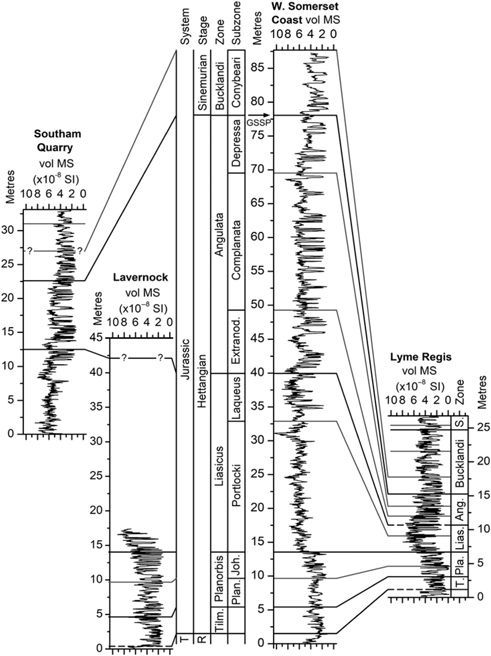

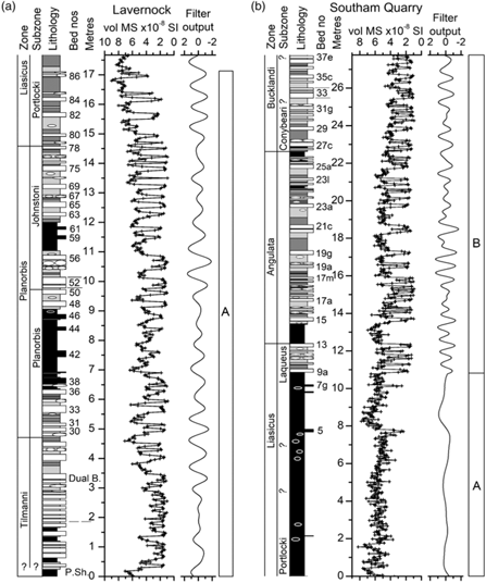

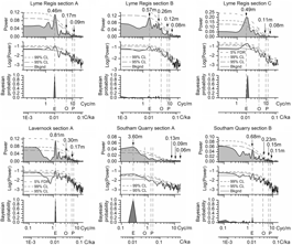

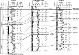


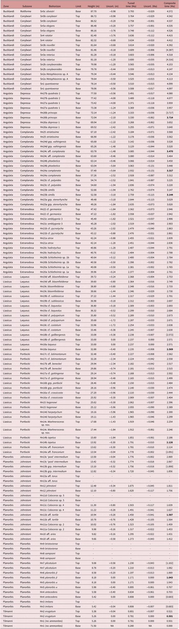
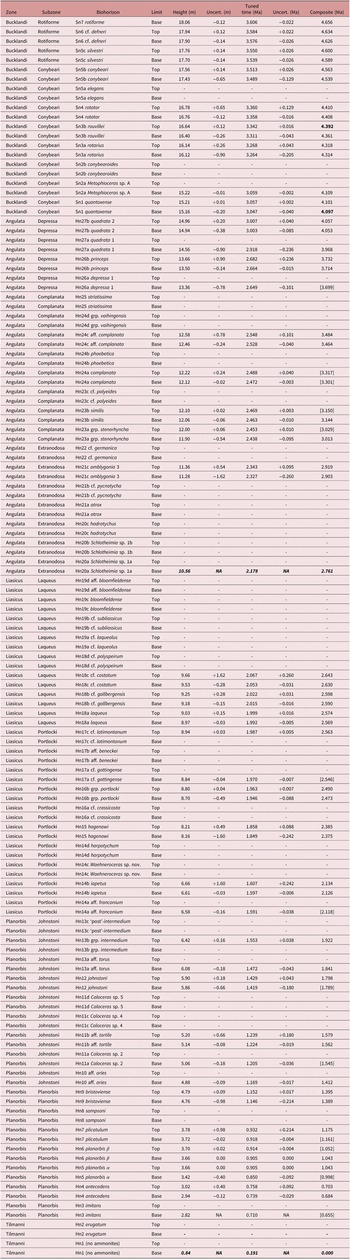


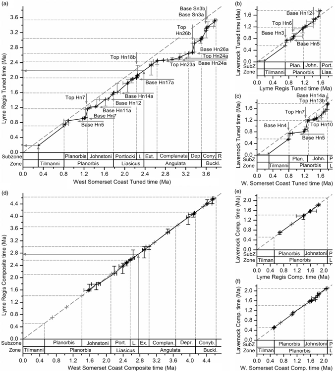


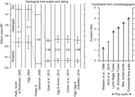

 Open access