Introduction
Cities, despite covering a small portion of the Earth, significantly impact biodiversity, resource consumption and greenhouse gas emissions (Madlener & Sunak Reference Madlener and Sunak2011). Urban green spaces, while not pristine habitats, are crucial for supporting regional and global biodiversity (Burrell et al. Reference Burrell, Evans and De Kauwe2020, Pörtner et al. Reference Pörtner, Scholes, Arneth, Barnes, Burrows and Diamond2023), providing vital ecosystem services (ESs) such as health benefits, climate regulation and socio-economic gains (Costanza et al. Reference Costanza, d’Arge, de Groot, Farber, Grasso and Hannon1997, Zhao & Lin Reference Zhao and Lin2024). Water resource regulation, underpinned by hydrological cycles, supports ecosystem health. Urban cooling mitigates heat island effects and climate change impacts. Air quality regulation reflects vegetation’s role in improving air quality. Carbon storage increases our carbon sequestration capacity for climate change mitigation. Vegetation productivity measures green space health and resilience to environmental pressures. These services underscore the multifaceted benefits of maintaining and enhancing green spaces within urban environments. New York City’s High Line Park demonstrates the substantial benefits of urban greening in developed areas (Zhang et al. Reference Zhang, Fan, Shrivastava, Homeyer, Wang and Seinfeld2022).
However, rapid urbanization has fragmented urban ecosystems, disrupting ecological processes and reducing ES supply (Geneletti & Zardo Reference Geneletti and Zardo2016). This fragmentation hinders species migration, degrades habitat quality and contributes to global biodiversity loss (Jung et al. Reference Jung, Arnell, de Lamo, García-Rangel, Lewis and Mark2021), indicating the need for sustainable urban development (McDonnell & MacGregor-Fors Reference McDonnell and MacGregor-Fors2016, Zeng et al. Reference Zeng, Koh and Wilcove2022, Neyret et al. Reference Neyret, Peter, Le Provost, Boch, Boesing and Bullock2023). Despite ecological restoration efforts, challenges such as resource constraints and human–ecological conflicts persist (Klaus & Kiehl Reference Klaus and Kiehl2021, Li et al. Reference Li, Wu, Hua and Mi2024), especially in rapidly urbanizing regions such as Beijing. Fragmentation-induced isolation further limits species migration and reproduction (Hooftman & Bullock Reference Hooftman and Bullock2012, Ribeiro et al. Reference Ribeiro, de Mello and Valente2022), exacerbating these challenges. Therefore, understanding the complex interplay between urbanization, biodiversity conservation, ES maintenance and ecological connectivity is crucial in rapidly changing landscapes.
Effective conservation planning requires balancing ecological features such as complementarity, comprehensiveness, representativeness and adequacy (Kukkala & Moilanen Reference Kukkala and Moilanen2013). Specifically, complementarity ensures that conservation areas fill ecological gaps: comprehensiveness ensures all major ecological types and species are included, representativeness ensures diverse ecosystems and species are protected and adequacy ensures that conservation areas are large enough and of high enough quality to be effective over the long term. While various spatial analysis methods exist (Geneletti & van Duren Reference Geneletti and van Duren2008, Pullinger & Johnson Reference Pullinger and Johnson2010, Zeng et al. Reference Zeng, Koh and Wilcove2022, Qian et al. Reference Qian, Zhao and Li2023), many inadequately address the trade-offs and synergies between ecological features such as habitat quality and ESs. Existing research highlights the potential alignment between biodiversity and carbon conservation (Nelson et al. Reference Nelson, Mendoza, Regetz, Polasky, Tallis and Cameron2009), but biodiversity-focused approaches often neglect socio-ecological values (He Reference He2020), while ES-centric planning may miss biodiversity synergies (Cimon-Morin et al. Reference Cimon-Morin, Darveau and Poulin2016). Furthermore, habitat quality-centric approaches may overlook areas that are critical for rare species (Bennett et al. Reference Bennett, Peterson and Gordon2009, Soto-Navarro et al. Reference Soto-Navarro, Ravilious, Arnell, De Lamo, Harfoot and Hill2020).
Maintaining landscape connectivity is vital for species dispersal, abundance and long-term viability (Ramel et al. Reference Ramel, Rey, Fernandes, Vincent, Cardoso and Broennimann2020). Fragmentation impedes movement, increasing extinction risks. Optimizing conservation strategies requires a careful evaluation of the trade-offs between ES supply, connectivity and biodiversity, particularly species abundance (O’Connor et al. Reference O’Connor, Pollock, Renaud, Verhagen, Verburg and Lavorel2021). China is among the 12 most biodiverse countries in the world, and Beijing is one of the most biodiverse megacities globally. Beijing, recognized as a ‘Biodiversity Charm City’ at CBD COP16 (Sixteenth Meeting of the Conference of the Parties to the Convention on Biological Diversity), offers a valuable opportunity to investigate urban biodiversity dynamics. In 2024, Beijing had already identified 612 terrestrial wild vertebrate species, of which birds alone constituted 519 species, as a critical node on the East Asia–Australia Migratory Bird Corridor, ranking second among G20 capital cities (Liu & Fu Reference Liu and Fu2019). Concurrently, 2088 species of vascular plants have been recorded, demonstrating the continuous improvement in Beijing’s biodiversity level (Beijing Municipal Ecology and Environment Bureau 2024). However, challenges such as habitat fragmentation and single-species plantations persist (Yang et al. Reference Yang, Zhou, Yu, Fan and Zhang2012) despite afforestation efforts, emphasizing the urgent need for effective conservation and landscape management, especially for threatened species along migratory routes (Zeng et al. Reference Zeng, Koh and Wilcove2022).
This study aims to develop a comprehensive, spatially explicit framework for conservation prioritization in rapidly urbanizing Beijing. By integrating multi-criteria spatial analysis, including ES supply modelling, landscape connectivity assessment and species distribution modelling, this framework identifies priority conservation areas and evaluates trade-offs. The resulting spatial prioritization map seeks to optimize landscape sustainability by balancing ecological and urban demands.
Methods
Study area
The study area is Beijing (39.9°N, 116.4°E), a globally significant megacity for biodiversity in northern China, encompassing 16 410 km2. Mountains in the north-west and west constitute 62% of Beijing, providing key habitats, while the south-eastern plains are densely urbanized, posing conservation prioritization challenges. Beijing experiences a temperate monsoon climate with hot, humid summers and cold, dry winters, receiving c. 600 mm of annual precipitation, mainly in summer. Significant climatic variations occur due to topography, with the mountainous regions being cooler and wetter than the plains. This altitudinal gradient shapes ecosystem and biodiversity distribution, being critical for conservation planning.
The Beijing Municipal Commission of Planning and Natural Resources (BMCPNR) has established ecological security patterns (ESPs) and nature reserves (Beijing Municipal Bureau of Gardening and Greening 2020, Beijing Municipal Government 2022). Ecological security theory informs ecosystem assessment and management (Yu Reference Yu1998). Currently, nature reserves cover 17% of Beijing’s area but only 0.3% of the metropolitan area, being insufficient for plains species conservation (Huang et al. Reference Huang, Gu, Yang and Wen2021). While achieving a 30% conservation target is geographically feasible due to mountainous regions, a more comprehensive goal is to protect the top 50% of high-priority areas across both mountains and urban zones (Beijing Municipal Government 2024). This balances ecological protection and development, preserving key habitats and biodiversity hotspots city-wide.
Assessment of ecosystem service supply
ES supply, defined as the benefits that ecosystems provide (Fang et al. Reference Fang, Xue, Zhou, Cheng, Bai and Huang2024), requires context-specific prioritization. Based on the Common International Classification of Ecosystem Services (CICES), the Beijing Urban Master Plan (2004–2020) and Beijing’s environmental challenges, we prioritized five key services: water resource regulation, urban cooling, carbon storage, air quality regulation and vegetation productivity. These services are crucial for biodiversity, ecosystem resilience and sustainable urban development (Cimon-Morin et al. Reference Cimon-Morin, Goyette, Mendes, Pellerin, Poulin and Fraser2021).
Water resource regulation service supply
We assessed hydrological services using InVEST models (Natural Capital Project 2024), specifically water yield and urban flood regulation. The water yield model estimated groundwater recharge and surface water flow distribution, which are crucial for regional water resources (Lu et al. Reference Lu, Sun, Feng and Fu2013). The flood risk regulation model assessed flood mitigation areas, being relevant to urban infrastructure and land use (Falter et al. Reference Falter, Dung, Vorogushyn, Schrter and Merz2016). Both models used precipitation, evapotranspiration, land use, soil and topography as inputs. Due to spatial overlap, we primarily focused on flood risk regulation for further analysis. The main calculation formulae are provided in Appendix S1.
Urban cooling service supply
Urban cooling service supply was assessed using land surface temperature (LST) as a key indicator, derived from MODIS, Landsat and Sentinel remote-sensing data (http://www.gisrs.cn/). LST was used to quantify the urban cooling service by reflecting the surface energy balance in the context of urban heat island analysis. We used an improved split-window algorithm for LST inversion (Rongali et al. Reference Rongali, Keshari, Gosain and Khosa2018) to retrieve LST data from spaceborne sensor infrared channels; this ensured precise LST estimations across urban and rural landscapes by incorporating atmospheric transmittance, surface emissivity and brightness temperature (Deng et al. Reference Deng, Wang, Bai, Tian, Wu and Xiao2018).
Carbon storage service supply
For carbon storage service supply, we calculated ecosystem carbon stocks from the carbon storage module of the InVEST model using land-use and carbon density data for different land-cover types (Yang et al. Reference Yang, Zhou, Yu, Fan and Zhang2012, Li et al. Reference Li, Guirui and Nianpeng2018). This process helped quantify the carbon stored in above-ground biomass, below-ground biomass, dead organic matter and soil. The formulae for calculating carbon density for each class are provided in Appendix S1.
Air quality regulation service supply
Air quality regulation service supply was assessed by focusing on particulate matter of <2.5 µm in diameter (PM2.5) dry deposition in green spaces (woodlands, grasslands, croplands). The capacity of green space structures (canopies, leaves, branches) to facilitate the dry deposition of atmospheric pollutants was used to assess the air quality regulation service. The removal quantity is considered to be dependent on the pollutant deposition rate and concentration. We used a dry deposition model (Chen et al. Reference Chen, Liu, Pan, Chen, Li and Wang2014) to calculate green space purification of PM2.5, excluding wet deposition. Model coefficients and the spatial distribution map are provided in Appendix S1.
Vegetation productivity service supply
To assess vegetation productivity service supply, we utilized net primary productivity (NPP) as a fundamental measure, reflecting the ecosystem’s capacity to produce biomass through photosynthesis. In this study, NPP serves as an indicator of the potential of green vegetation to support various ecosystem functions. In this study, NPP was assessed using MODIS data and calculated via the Carnegie–Ames–Stanford Approach (CASA) model (Field et al. Reference Field, Randerson and Malmström1995). Data requirements for the CASA model included land cover, Normalized Difference Vegetation Index (NDVI) and climate data. This calculation enabled the generation of spatial maps depicting the NPP distribution across the study area, thereby identifying regions with varying levels of vegetation productivity service supply capacity (see Appendix S1).
Landscape connectivity
To evaluate landscape connectivity comprehensively (Luque et al. Reference Luque, Saura and Fortin2012, Wang et al. Reference Wang, Qu, Zhong, Zhang, Zhang and Zhang2022), we used three complementary methods: the Integral Index of Connectivity (IIC); minimum cost resistance (MCR); and morphological spatial pattern analysis (MSPA) and the contagion index (CONTAG).
The IIC was employed to quantify the contribution of each habitat patch to overall landscape connectivity by evaluating patch size and connection strength (Pascual-Hortal & Saura Reference Pascual-Hortal and Saura2008). In this study, the IIC was used to assess how fragmentation impacts the potential for species movement across the urban landscape. We calculated the IIC using Conefor Sensinode (Saura & Torné Reference Saura and Torné2009), representing the landscape as a network of nodes (patches) and edges (connections), to assess both habitat connectivity and relative quality.
MCR employed a cost surface based on land cover and terrain to represent movement resistance, derived from the Beijing Urban Master Plan (2016–2035), with a focus on ecological sources and sinks. It calculated cumulative resistance from a source to any point, with lower values indicating higher accessibility and movement potential, thus informing landscape function analysis. MCR model details are given in Appendix S1.
MSPA classifies foreground pixels into seven mutually exclusive types: Core, Islet, Edge, Perforation, Bridge, Loop and Branch, each with indicative significance for landscape connectivity (Pedroli et al. Reference Pedroli, Pinto-Correia and Cornish2006). We used GuidosToolbox (Vogt et al. Reference Vogt, Riitters, Rambaud, D’Nnunzio, Lindquist and Pekkarinen2022) and ArcGIS 10.2 for this analysis. Green landscapes (forests, grasslands, wetlands, water bodies, urban green spaces) were extracted from land-use data as foreground; other areas were background. The analysis used a 30-m pixel size and eight-neighbour algorithm.
CONTAG was used to quantify the landscape pattern of Beijing using FRAGSTATS 4.3 (McGarigal et al. Reference McGarigal, Cushman, Neel and Ene2002), employing a method combining moving window analysis and gradient analysis. Among these, CONTAG was selected. CONTAG describes the degree of aggregation or dispersal of different patch types within a landscape (Zou et al. Reference Zou, Wang and Bai2022). Generally, a higher CONTAG value indicates greater connectivity among dominant patch types.
Habitat potential for threatened species
Habitat suitability for threatened species was modelled using MaxEnt, a maximum entropy-based machine learning approach (Guillera-Arroita et al. Reference Guillera-Arroita, Lahoz-Monfort, Elith, Gordon, Kujala and Lentini2015). MaxEnt models species distributions by estimating the most uniform distribution of their presence, constrained by environmental variables and occurrence points.
For key Beijing species, we compiled a dataset via species selection, data acquisition and refinement. Species selection, from Beijing protected species lists and conservation plans (2008–2035), identified 366 indicator species (19 amphibians, 266 birds, 30 mammals, 70 plants) based on endangered status, protection level and endemism. Historical spatial distribution data came from the Global Biodiversity Information Facility (GBIF), the China Biodiversity Map and the China Birdwatching Record Center. The dataset included species information, conservation status and coordinates.
Dataset refinement standardized coordinates, removed duplicates and filtered for species with ≥10 distribution points in Beijing (Pellissier et al. Reference Pellissier, Schmucki, Pe’er, Aunins, Brereton and Brotons2020), resulting in 65 species (7 amphibians, 19 birds, 24 mammals, 15 plants) in CSV format (Appendix S1, Tables S2–S5). Bias was addressed by: (1) checking for clustering; (2) accounting for sampling bias; (3) using bias layers from kernel density maps for background weighting; (4) area under the curve (AUC) and response curve model evaluation; and (5) visual inspection.
Environmental predictors included 25 variables: 19 climatic, 4 habitat-related and 2 human impact-related (Huang et al. Reference Huang, Zhao, Li and von Gadow2015). MaxEnt was run with default settings, a 75% training/25% validation split (Merow et al. Reference Merow, Smith and Silander2013), 10 bootstrap replicates and logistic output.
Scenario design and Zonation analysis
To compare conservation objectives, we defined four scenarios: (1) ES supply only (ESS-only): five ESs (carbon storage, etc.; w = 1); (2) landscape connectivity only (LC-only): connectivity indices (IIC, MCR, MSPA, CONTAG; w = 1); (3) habitat potential for threatened species only (HPTS-only): habitat suitability for 65 threatened species (w = 1); and (4) all equal: equal weights (w = 1) to ES supply, connectivity and threatened species habitat. Equal weighting was applied after aggregating the five ES supply, four connectivity indicators and 65 species into respective indices (Kujala et al. Reference Kujala, Lahoz-Monfort, Elith and Moilanen2018).
We used Zonation 5.0 with the Core Area Zonation (CAZ2) removal rule (Moilanen et al. Reference Moilanen, Kujala and Mikkonen2020) to optimize spatial prioritization, aiming for feature balance and complementarity, and we restricted prioritization to 50% of the landscape, aligning with city targets. Spatial prioritization in Zonation uses a marginal loss rule, aggregating conservation value loss across features via a p-norm on weighted feature distribution fractions within a cell. The marginal loss for cell i is calculated as in Equation 1. CAZ2 is a key Zonation method. Unlike additive benefit functions, CAZ derives spatial solutions from data and prioritization rules. CAZ2 (L2 norm/Euclidean distance) balances the performance and representation of limited-distribution features (Moilanen et al. Reference Moilanen, Lehtinen, Kohonen, Jalkanen, Virtanen and Kujala2022), and it was chosen over CAZ1 and CAZP for its balance.
 $${M_i} = {\left( {\mathop \sum \nolimits_{j=1}^n {{\left| {{w_j}{r_{ij}}} \right|}^p}} \right)^{{1}\over{p}}}$$
In Equation 1, M
i
denotes the marginal biodiversity loss associated with the hypothetical removal of cell I, ${r_{ij}}$
is the fraction of feature j’s distribution remaining in cell i and
${r_{ij}}$
is the fraction of feature j’s distribution remaining in cell i and ${w_j}$
is the weight assigned to feature j. p is the order of the p-norm that controls the sensitivity of the aggregation. Larger values of p give more weight to the most affected features, whereas smaller values result in a more balanced contribution across all features. Weights were used to account for both positively and negatively weighted features.
${w_j}$
is the weight assigned to feature j. p is the order of the p-norm that controls the sensitivity of the aggregation. Larger values of p give more weight to the most affected features, whereas smaller values result in a more balanced contribution across all features. Weights were used to account for both positively and negatively weighted features.
In the Zonation analysis, all features from the three groups – ES supply, connectivity and threatened species habitat – were included as individual layers. We assigned equal weights to the three groups. Within each group, all layers were also weighted equally, ensuring that each feature contributed proportionally to its group-level weight.
Top 10%, 30% and 50% priority areas were extracted from each scenario for overlap and coverage assessments.
Gap analysis
To evaluate our conservation prioritization against Beijing’s official ecological management, we used the BMCPNR’s three-tiered ESP, which has three control zones: First-level (Bottom-line), Second-level (General) and Third-level (Ideal), guiding differentiated management policies based on ecological priority and land-use activities. The Bottom-line (First-level) zone strictly protects critical ecological areas (26.45% of Beijing), including major river corridors, wetlands and core forests, preventing irreversible degradation. The General (Second-level) zone enhances ecosystem functionality and maintains healthy conditions (41.29% of Beijing), being aligned with broader spatial planning. The Ideal (Third-level) zone involves proactive, flexible management (68.55% of Beijing), optimizing green space networks and multifunctional landscapes for conservation, economic and recreational uses.
These tiers represented graduated ecological safeguards from most to least restrictive. We overlaid our Zonation conservation priorities with the ESP tiers to identify whether priority areas for threatened species, ES supply and connectivity are within ESP designations or whether under-protected priority areas remain, especially within the metropolitan region.
Results
Spatial distribution of ecosystem service supply features and priority zones
ES supply exhibited spatially heterogeneous patterns across Beijing. Flood risk mitigation was generally higher in mountainous regions, but it also was significant in the south-eastern/north-eastern plains (Appendix S1, Figs S1 & S2), suggesting localized landscape influences or drainage infrastructure. Water resource regulation increased from the urban core outwards. Urban cooling was highest in mountainous areas, large reservoirs and peri-urban/suburban green spaces (Appendix S1, Fig. S3).
Carbon storage was concentrated in western/north-western Beijing, especially the north-western protective forest belt (Appendix S1, Fig. S4). Lower carbon storage was observed in the central/eastern plains, including the urban core and on built-up land. Air quality regulation demonstrated a greyscale gradient (Appendix S1, Fig. S5), with higher supply (lighter tones) in the north-western woodlands and the lowest supply in dense urban/industrial/high-traffic zones (darker tones). Vegetation productivity decreased from the north-western mountains to the urban centre and the south-eastern plains (Appendix S1, Fig. S6), with the highest productivity observed in the north-western woodlands (lightest tones) and lowest productivity observed in urban built-up/industrial areas (darkest tones).
The Zonation analysis prioritizing the top 10% ES supply areas identified the highest-priority zones (top 10%, deep blue) as concentrated and continuous in the north-western mountains (Fig. 1a). The top 10% ES supply zones were also discernible along the central plain river corridors. A decreasing priority gradient extended outwards through the top 10–30% (blue-green), top 30–50% (green) and lower zones (yellow, orange, brown). The lowest priority (bottom 10%, brown) was in the urban core. Zonation reinforced the individual ES analyses, confirming the north-western mountains’ importance for multi-functional ESs and the strategic value of urban riverine zones.

Figure 1. Spatial priorities based on single-factor scenario analyses. (a) Priority areas based solely on ecosystem service (ES) supply, aggregated from carbon storage, water resource regulation, urban cooling service, carbon storage service, air quality regulation service and vegetation productivity. Higher values (in darker shades) denote stronger ES supply. (b) Priority areas based solely on landscape connectivity, calculated via IIC/MCR/MSPA/CONTAG (see text for definitions). Darker regions indicate greater connectivity importance. (c) Priority areas based solely on habitat potential for threatened species (MaxEnt-derived suitability). Darker shades represent higher conservation value, while lighter shades indicate lower suitability. ‘High’ denotes the top percentile of priority cells (e.g., top 10%), and ‘Low’ denotes the bottom percentile.
Connectivity and key ecological patches
Connectivity analysis showed priority areas aligned with higher ecological integrity. Small ecological patches (<1 km2) were most numerous (58.85%), but medium (1–3 km2) and large patches (3–10 km2) significantly contributed to total area (30.60% and 28.98%, respectively). Mega-patches (>10 km2), although rare (Yongding, Wenyu and Chaobai River Parks), had disproportionately high connectivity (21.82%, 27.66% and 25.38%, respectively) due to their size, location and quality, being crucial for landscape connectivity (Appendix S1, Fig. S7).
The MCR model identified three primary ecological corridors in Beijing, mainly in the north-western mountains and extending south-east (Appendix S1, Fig. S8). Urban and agricultural areas showed the highest movement resistance, whereas forests and wetlands showed the lowest such resistance. Corridors totalled c. 500 km, connecting major forest patches and protected areas.
The MSPA results (Appendix S1, Fig. S9) showed the ‘Core’ landscape as large habitat patches and ecological sources. The ‘Edge’ was the transitional zone with high exchange. ‘Bridge’, ‘Branch’ and ‘Loop’ types acted as corridors. The contributions to connectivity ranked as follows: Core > Edge > Bridge > Branch > Loop. The ‘Core’ was mainly mountain forests and large rivers, the ‘Bridge’ was medium/small rivers, the ‘Branch’ connected the Core to surroundings and the ‘Loop’ enhanced the Core’s internal connectivity.
There were high landscape CONTAG index values (Appendix S1, Fig. S10, dark blue/green; 62.3–99.8) concentrated in the north-western/western mountains and some urban south-western patches, indicating aggregated, highly connected landscapes.
The Zonation analysis for integrated connectivity (Fig. 1b) prioritized the top 10% of areas for four connectivity metrics that were most critical for connectivity. The top 10–30% of zones (green/blue) extended from core areas, forming broader networks, especially along mountains and river valleys.
Spatial patterns of threatened species
The MaxEnt models for 65 threatened species showed varying performance (Appendix S1, Tables S7–S10). Most species (61.5%, 40 species) had excellent predictive performance (AUC > 0.9), 30.8% (20 species) had good predictive performance (AUC 0.8–0.9), and 7.7% (5 species) had moderate predictive performance (AUC 0.7–0.8). No species had poor predictive performance (AUC < 0.7). Detailed results and species maps are given in Appendix S1, Fig. S12.
The Zonation analysis (Fig. 1c) indicated high-biodiversity priority areas in both the central plains and north-western mountains. In the plains, high-priority zones were observed in north-western/northern urban areas (e.g., Olympic Forest Park). In the mountains, high-priority zones included Miyun Reservoir, Western/Fragrant Hills and Baihua Mountain. Low-priority plain areas were the outer suburbs (e.g., Daxing, Tongzhou, Shunyi Districts). Low-priority mountain areas were Labagou and the farmland north of Miyun Reservoir. Woodlands were the largest habitat type (54.80% of threatened species habitat), and built-up land accounted for 22.89%.
Gap analysis
Overlays of Zonation top-priority areas (10% and 30%) with Beijing’s ESP revealed limited alignment, especially in the metropolitan area. ESP Bottom-line, General and Ideal patterns showed low coverage of top-priority zones.
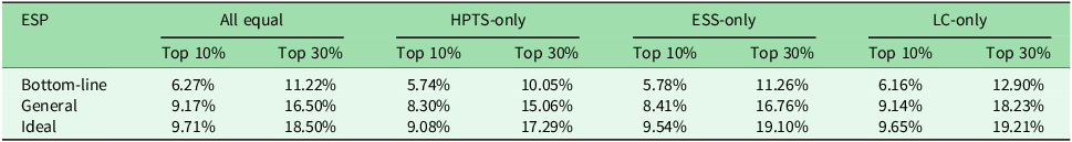
In the all equal scenario, the Bottom-line ESP covered only 6.27% of the top 10% priority areas (11.22% for the top 30%; Table 1). The Ideal ESP offered slightly better coverage (9.71% and 18.50% for the top 10% and 30%, respectively), but still leaving substantial under-protected areas. Similar low coverage trends were observed for the HPTS-only, LC-only and ESS-only scenarios with the Bottom-line ESP (Table 1).
Table 1. Spatial coverage and ecological value of top 10% and top 30% priorities in the assessed scenarios in Beijing.

ESS = ecosystem services supply; HPTS = habitat potential for threatened species; LC = landscape connectivity.
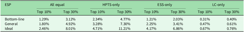
ESP overlap within the metropolitan area was even lower (Table 2). For the all equal scenario, Bottom-line ESP covered only 1.29% of the top 10% priority areas (3.12% for the top 30%). The Ideal ESP still only covered 2.46% of the top 10% zones and 8.01% of the top 30% zones. Consistently low spatial congruence in the metropolitan region was observed across all ESPs and scenarios (Table 2).
Table 2. Spatial coverage and ecological value of the top 10% and top 30% priorities in the optimal scenario in the metropolitan area of Beijing.

ESP = ecological security pattern; ESS = ecosystem services supply; HPTS = habitat potential for threatened species; LC = landscape connectivity.
ESP overlaps were spatially uneven, being concentrated in mountainous regions, especially in the ESS-only and LC-only scenarios (forested land cover). Plains overlaps were limited, with the HPTS-only scenario showing some overlap at Hanshiqiao Wetland and Huaijiu River (riverine wetlands). The all equal scenario showed sparse overlaps at scenic/World Heritage sites and in the Grand Canal regions (Appendix S1, Figs S13–S16).
In conclusion, Beijing’s ESP showed limited spatial congruency with high-priority conservation areas, particularly in metropolitan areas. The ESP and nature reserves alone were found to be insufficient to protect key ecological features, especially in urbanized plains and urban green spaces.
Conservation prioritization
High ES supply areas in the north-west partially co-occurred with biodiversity and connectivity priorities (Fig. 1). As revealed by the Zonation-based prioritization analysis, there was limited spatial overlap among the top 10% priority areas for the three criteria (Fig. 2). For example, there was only 0.62% overlap between the top 10% ES supply and connectivity areas, contrasting with 2.57% overlap between the biodiversity and ES supply top 10% zones, indicating spatial synergy. Biodiversity and urban areas showed a 1.71% overlap in the top 10% of zones, suggesting conflict. Overlap increased when considering the top 30% priority zones: 7.44% for biodiversity–urban (conflict) and 12.70% for biodiversity–ES supply (synergy). The top 10% overlap among all three features was only 0.19%, and the top 30% was 5.29%, highlighting trade-offs (Fig. 3b). These maps, derived from Zonation performance outputs, indicated potential conflicts and synergies, necessitating balanced conservation prioritization.

Figure 2. Spatial conflicts between multiple design criteria in Beijing. This heatmap compares the overlap percentages of the top 10% or top 30% priority areas among four distinct single-factor scenarios and the all equal scenario (HPTS = habitat potential for threatened species; ESS = ecosystem service supply; LC = landscape connectivity; all equal = integrated weighting). Diagonal from top-left to bottom-right represents the same scenario (no comparison), while off-diagonal cells indicate pairwise overlaps: for instance, 2.57% means that only 2.57% of the top-priority area under HPTS overlaps with the top-priority area under ESS. The colour scale (light blue to dark blue) shows increasing percentages of overlap. Low overlap values (<5%) highlight trade-offs between these design criteria, whereas higher overlaps (>20%) suggest potential synergies or similar priority zones.

Figure 3. Priority maps for (a) Beijing and (b) performance curves based on the analysis considering all three major criteria jointly. (a) Zonation-integrated scenario incorporating all major ecological features (i.e., threatened species habitat, ecosystem service (ES) supply and landscape connectivity with a positive weight). Areas in blue and green are of higher conservation priority, while areas in orange and red are of lower priority. The black outline indicates Beijing’s municipal boundary. (b) The x-axis represents the fraction of landscape lost from conservation, priority ranked from 0 (lowest) to 1 (highest). For instance, the top 30% of the landscape corresponds to ranks 0.7–1.0. The y-axis represents what remains for that feature in terms of coverage fraction of the selected feature (from 0 to 1), indicating how much of that feature (e.g., total habitat, connectivity value) is captured at a given priority threshold. Curves correspond to priority areas based on ES supply only (blue), landscape connectivity only (orange), biodiversity only (grey) or all four ecological features weighted equally (yellow). At a rank of 0.7 (top 30%), the habitat curve (grey) suggests that 77.5% of threatened species habitat is covered, indicating a relatively compact distribution.
The top 10% priority areas (Fig. 3a, dark blue) were mainly in key biodiversity and ecologically sensitive regions such as Wenyu/Sha River corridors and Imperial/Fragrant Hills. Medium- to high-priority areas (top 10–50%, green shading) were extensive in the northern/western mountains due to their undisturbed habitats. Lower-priority zones (bottom 10–50%, yellow-orange) were concentrated in central urban/south-eastern plain regions due to development pressures. This spatial pattern emphasized balancing conservation in high-priority zones with sustainable development in lower-priority areas.
Performance curves
Among the performance curves for the ESS-only, LC-only, HPTS-only and all equal scenarios, the HPTS-only scenario consistently achieved the highest coverage; the top 30% priority conservation areas captured >77.5% of threatened species habitat, demonstrating high efficiency (Fig. 3b). The ESS-only and LC-only scenarios showed lower coverage of the top 30% priority conservation areas (61.5% and 49.0%, respectively), indicating connectivity’s more diffuse distribution and less concentrated priority ranking.
The all equal curve showed moderate trade-offs, achieving c. 65.0% coverage of the top 30% priority conservation areas. Expanding conservation to 50% increased efficiency for all scenarios: all equal to >82.5%, ESS-only to 85.3%, LC-only to 74.9% and HPTS-only to 92.6%, with the curves then levelling off. Combined with Fig. 3a, this suggested expanding from a 30% to a 50% target includes mountainous regions to a significant extent, enhancing overall efficiency and supporting broader ecological sustainability across diverse landscapes.
Discussion
Our findings offer insights into ecological assets in a rapidly urbanizing megacity and considerations for balancing conservation and development.
Limited spatial overlap and trade-offs among conservation priorities
Spatial prioritization methods have been extensively developed, particularly for natural and semi-natural ecosystems, such as mountains and forests. However, there has been less focus on highly urbanized and socio-ecologically complex areas such as megacities. Previous studies have explored various frameworks for spatial prioritization, such as integrating ESs and biodiversity in the Alps (Ramel et al. Reference Ramel, Rey, Fernandes, Vincent, Cardoso and Broennimann2020), assessing ES potential across the European Union (Vallecillo et al. Reference Vallecillo, Polce, Barbosa, Perpiña, Vandecasteele, Rusch and Maes2018) and incorporating multi-hazard risks in rapidly urbanizing regions (Ou et al. Reference Ou, Lyu, Liu, Zheng and Li2022). Additionally, frameworks that combine biodiversity and carbon storage at a continental scale have been proposed (Zhu et al. Reference Zhu, Hughes, Zhao, Zhou, Ma and Shen2021). In contrast to natural areas, urban environments face greater complexity in prioritization due to rapid urbanization and habitat degradation.
The limited spatial overlap among high-priority areas for biodiversity, ES supply and connectivity (Fig. 2) highlighted the inherent trade-offs in urban–rural landscapes, especially within the top 10% zones. Minimal ES supply and connectivity overlap (0.62%) suggested that areas for water purification/carbon sequestration differ from species movement corridors. The higher biodiversity and ES supply overlap (2.57%) indicated potential synergy, possibly from co-occurring forests. However, even synergistic overlaps were modest, challenging integrated conservation within limited space. These findings align with the broader literature on trade-offs and mismatches among ESs and biodiversity priorities (Xiang et al. Reference Xiang, Zhang, Mao, Wang, Qiu and Yan2022, Shen et al. Reference Shen, Li, Wang, Wu, Liang and Zhang2023).
The performance curves (Fig. 3b) further illustrated these trade-offs. The HPTS-only scenario showed the highest efficiency for threatened species, but single-objective prioritization reduced performance for ES supply and connectivity. The all equal scenario reflected a compromise. The levelling off of the performance curves at the 50% target suggested that broader expansion into less concentrated regions (mountains) is needed for ecological sustainability, with diminishing efficiency gains. These curves offer quantitative insights for Beijing’s decision-makers regarding balancing conservation objectives and resource allocation, echoing performance curve utility in conservation prioritization (Fu et al. Reference Fu, Ding, Sun and Xu2021, Hijriyah et al. Reference Hijriyah, Utami, Hasanah, Kurniawan, Putri and Nuraeni2024).
Implications for Beijing’s ecological security pattern and urban green space management
Our gap analysis showed limited spatial congruence between Beijing’s ESP and our identified high-priority conservation areas, especially in the urban metropolitan region (Table 2). This raises concerns regarding the ESP’s effectiveness for protecting critical areas for threatened species, ES supply and connectivity, particularly in fragmented urban areas. While the ESP showed some overlap in mountains/forests, low metropolitan coverage was found to be where urban/peri-urban ecological assets are under-represented in the ESP framework. This is a critical gap, especially given urban green spaces’ increasing ecological importance in fragmented landscapes (Bourgeois et al. Reference Bourgeois, Boutreux, Vuidel, Savary, Piot and Bellec2024).
Beijing’s ESP needs refinement to better incorporate high-priority conservation areas, especially in the metropolitan region. This could involve: (1) strengthening urban/suburban green space protection (river corridors, parks, peri-urban forests) due to their disproportionate urban importance; (2) re-evaluating ESP criteria, potentially using our multi-criteria approach and gap areas; and (3) developing targeted, spatially explicit conservation policies for different landscape zones, moving beyond a one-size-fits-all approach.
Limitations and future directions
This supply-focused study, while novel and sufficiently spatially robust for Beijing’s conservation priorities, omits ES demand and complex flow processes, which future research should integrate for holistic, policy-relevant insights. Furthermore, although the 65 species assessed here represent key threatened taxa, their restricted taxonomic scope (primarily vertebrates and flagship flora) may inadequately capture broader biodiversity patterns. Expanding the scope to cultural services, health and climate resilience would improve the comprehensiveness of this research. Longitudinal studies are crucial to monitor policy effectiveness and urbanization/climate change impacts.
Despite these limitations, we provide a methodologically novel and spatially robust multifaceted assessment of conservation priorities in a megacity. Our approach highlighted the spatial heterogeneity of ecological assets, the trade-offs among different conservation objectives and the critical gaps in existing ESPs, particularly within the metropolitan region. We also provide an unprecedentedly detailed assessment of Beijing. Our findings underscored the need for a more nuanced and integrated approach to conservation planning in rapidly urbanizing megacities such as Beijing, one that effectively balances the protection of essential ecological features with the pressures of urban development. For management, our research directly informed the spatial targeting of conservation efforts by providing a spatial prioritization map that can be directly implemented in urban green space planning to maximize biodiversity and ES co-benefits, or by identifying critical ecological corridors that require urgent protection or restoration. By identifying key priority areas, highlighting the limitations of current conservation strategies and demonstrating the effectiveness of novel combinations of landscape connectivity metrics, biodiversity and ES trade-off analysis using Zonation CAZ2, this research makes a significant contribution to conservation prioritization methodologies for informing more effective and spatially targeted conservation policies in Beijing and other similar urbanizing regions worldwide.
Conclusions
We highlight the conservation prioritization challenges in Beijing of balancing biodiversity, ES supply, connectivity and urban development. Spatial analysis revealed distinct patterns: carbon storage and water supply being concentrated in the north-western mountains, while biodiversity hotspots were spatially dispersed and notably present in some urbanized areas. Gap analysis showed limited ESP coverage (9.6% of the top 10% priority zones), therefore needing improved alignment. The performance curves highlighted targeted threatened species habitat protection efficiency (83% of biodiversity in the top 30% priority areas), with expanded 50% protection enhancing overall coverage. An integrated strategy prioritizing under-protected urban and rural areas is crucial for ecological gap closure and sustainable urban growth in Beijing.
We thus provide a robust spatial framework for conservation prioritization in urbanizing megacities such as Beijing. Integrated assessment revealed that while Beijing’s mountains were vital for multi-functional assets, spatial mismatches existed between the ESP and high-priority zones, especially in the urban core. A refined, spatially targeted strategy extending beyond current protected areas is urgently needed to safeguard urban and peri-urban biodiversity and ecological functions. This research contributes to a nuanced understanding of urban ecological security and offers actionable guidance for balancing urban development with global biodiversity conservation.
Supplementary material
To view supplementary material for this article, please visit https://doi.org/10.1017/S0376892925100076.
Acknowledgements
None.
Financial support
This research was funded by the National Natural Science Foundation of China, grant number 41901220, the General project of Beijing Municipal Science & Technology Commission (KM201910016018) and Youth Backbone Individual Program of Beijing Excellent Talents Training Project.
Competing interests
The authors declare none.
Ethical standards
Not applicable.