ICESat data and processing

The Geoscience Laser Altimeter System (GLAS) on board ICESat (Reference Schutz, Zwally, Shuman, Hancock and DiMarzioSchutz and others, 2005) sampled 50–70 m diameter footprints every ∼172 m along each track, with elevation retrieval precision and accuracy of ∼2 and ∼14 cm, respectively (Reference ShumanShuman and others, 2006). ICESat’s southern limit of 86° S meant that it sampled all of Antarctica’s floating ice shelves. Between October 2003 and October 2009 when data acquisition ceased, ICESat operated in ‘campaign’ mode two or three times per year (Reference Schutz, Zwally, Shuman, Hancock and DiMarzioSchutz and others, 2005) with discrete 33 day data acquisition periods capturing the same 33 day sub-repeat cycle of a 91 day exact repeat cycle.

Our approach to estimating the GZ using ICESat repeat-track altimetry closely follows the technique described by Reference Fricker and PadmanFricker and Padman (2006) and used by Reference Fricker, Coleman, Padman, Scambos, Bohlander and BruntFricker and others (2009) and Reference Brunt, Fricker, Padman, Scambos and O’NeelBrunt and others (2010) for mapping the GZs of the Amery and Ross ice shelves, respectively. Specifically, we used GLA12, Release 428 data for the 17 ICESat campaigns between October 2003 and October 2009. We converted the ICESat locations and elevations from the TOPEX/Poseidon ellipsoid to the World Geodetic System 1984 (WGS84) ellipsoid (for consistency with other polar altimetry datasets) and applied the saturation corrections provided in GLA12. Finally, we applied our ‘rejection criteria’, which included the removal of tracks based on cloud cover and large cross-track offset. Specifically, we removed cloud-affected tracks, based on high gain values and low return energy levels. We then removed repeated passes with large cross-track offsets (greater than ∼100 m) and interpolated along-track data to a nominal reference track whose location was the average of all the repeated passes (Reference Brunt, Fricker, Padman, Scambos and O’NeelBrunt and others, 2010).

The uncertainties associated with cross-track error depend on the amount of track offset and the surface slope. While more sophisticated techniques have been developed to correct for these errors (e.g. Reference Smith, Fricker, Joughin and TulaczykSmith and others, 2009; Reference GardnerGardner and others, 2011; Reference ZwallyZwally and others, 2011), we do not use those methods here since the assumption of time-independent cross-track slope is not valid in the GZ and since they are more suited to the low-surface-slope regions of the ice-sheet interior, where the slopes are more uniform along repeat-track segments.

The GLA12, release 428, elevations have had predicted ocean and load tides removed using the GOT99.2 global ocean-tide model; however, identification of GZ features using repeat-track analysis is dependent on detecting the ice-shelf tidal response. Therefore, we ‘re-tided’ these elevations, i.e. removed the applied tidal correction from the GLA12 elevations (Reference Fricker and PadmanFricker and Padman, 2006). Maximum tidal range is typically 1–2 m for Antarctica but is up to ∼8 m in the southwestern corner of the FRIS (Reference Padman, Fricker, Coleman, Howard and ErofeevaPadman and others, 2002).

Estimation of grounding zone points

We performed ICESat repeat-track analysis on a track-bytrack basis, following the method described by Reference Brunt, Fricker, Padman, Scambos and O’NeelBrunt and others (2010). We first approximately located the FRIS GL visually, using the GL from MOA (J. Bohlander and T. Scambos, http://nsidc.org/data/atlas/news/antarctic_coastlines.html) overlaid on MODIS MOA imagery (Reference Scambos, Haran, Fahnestock, Painter and BohlanderScambos and others, 2007). For each track, we extracted the segment of the track that straddled the GL and then applied our rejection criteria. We interpolated the remaining repeated passes to a center-line reference track, using an along-track interpolation interval of 200 m. We determined a mean along-track elevation profile, h_i (x), and defined the ‘elevation anomaly’, , for each repeated pass as the difference of each elevation profile from h_i (x); this is the same as referencing the profiles to a zero mean. This procedure resulted in a set of elevation anomaly profiles for each track.

The method of estimating the GZ points for each ICESat track is illustrated in Figure 2. For each track, we located point I_b (the break-in-slope) by examining the shape of the surface topography in the set of ICESat elevation profiles (Fig. 2a, top panel); it is usually within ∼2 km of the MOA GL estimate. For this study, we are mapping more features of the GZ than MOA is capable of; however, with respect to our focus on ice plains, we are also interested in the regions where the separation of MOA and ICESat GL points is >2 km.

Fig. 2. Example of the estimation of GZ parameters (points I_b, F, H and C) from ICESat repeat-track analysis applied to two tracks that cross the FRIS GZ approximately normal to the MOA GL (see Fig. 3 for track locations). (a) Track 25, near Carlson Inlet. Top: set of ‘re-tided’ ICESat surface elevation profiles relative to WGS84 ellipsoid for all valid repeated passes of track 25. Bottom: set of elevation anomalies, calculated by subtracting the reference elevation profile (i.e. the mean of all elevation profiles) from the individual elevation profiles. At the right are the tide height predictions from the CATS 2008a tide model (also referenced to zero mean; Reference Padman, Fricker, Coleman, Howard and ErofeevaPadman and others, 2002) that correspond to each repeated pass. (b) Track 153, across a known ice plain near Institute Ice Stream. Top: similar to (a) but, in the presence of an ice plain, the first break-in-slope is the coupling point, C. Bottom: as in (a); however, point F migrates several kilometers with the tide, through the range delimited by F1 and F2.

We estimated points F and H from analysis of the set of elevation anomaly profiles (Fig 2a, bottom panel). For each track, we used the latitude and longitude associated with point I_b, and the times of each repeated pass, to predict the tidal heights using the Circum-Antarctic Tidal Simulation version 2008a (‘CATS 2008a’), an update to the inverse model reported by Reference Padman, Fricker, Coleman, Howard and ErofeevaPadman and others (2002). Predictions were made for the nearest water point in the CATS2008a 4 km grid. Tidal height predictions facilitate the estimation of points F and H in the elevation anomaly profiles by distinguishing tidal signal from other sources of elevation anomalies such as sampling of static topography by nonexact repeated tracks, accumulation or dynamic thinning (Reference Brunt, Fricker, Padman, Scambos and O’NeelBrunt and others, 2010). We interpret the region where the elevation anomaly is close to zero (Fig. 2a, bottom panel, to the left of point F) as fully grounded ice, and the region where the elevation anomaly is close to the tidal predictions (Fig. 2a, bottom panel, to the right of point H) as freely floating (hydrostatic) ice shelf.

If an ice plain is present, there is often more than one break-in-slope, making our interpretation of the ICESat repeat-track data slightly more complex. On ice plains, point C, the coupling point described by Reference Corr, Doake, Jenkins and VaughanCorr and others (2001), is generally the first break-in-slope in the vicinity of the GZ. Figure 2b, top panel, illustrates this for track 153, across an ice plain in the mouth of Institute Ice Stream. Ice plains also make the estimation of point F more difficult, as the typically low bedrock slopes allow point F to migrate longitudinally several kilometers with the tide; F1 in the bottom panel of Figure 2b is an estimate of point F from a set of repeated passes made at low tidal states, while F2 is an estimate made from repeated passes at high tidal states. The difference between the two estimates of point F (F1 and F2) in this example is ∼2 km.

The two tracks used as examples in Figure 2 cross the FRIS GZ approximately normal to the MOA GL. For tracks that cross the GL obliquely, care is required when interpreting GZ structure and time dependence from relative along-track distances of specific features.

Mapping the FRIS grounding zone

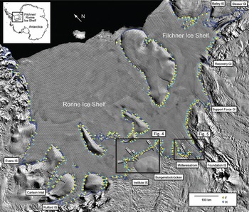
We estimated the location of 431 sets of GZ points (I_b, F and H) for the FRIS, including its perimeter, islands and ice rises (Fig. 3). The FRIS GZ is included in a continent-scale, ICESat-derived GZ dataset (K.M. Brunt and others, http://nsidc.org/data/nsidc-0469.html). These discrete GZ estimates have also been used in conjunction with Landsat-7 Enhanced Thematic Mapper Plus imagery to create a continuous, high-resolution Antarctic GL dataset, which describes the loci of points H and I_b (Reference BindschadlerBindschadler and others, 2011; R. Bindschadler and others, http://www.nsidc.org/data/nsidc-0489.html).

Fig. 3. Estimated locations of ICESat-derived GZ surface features (point F, yellow, and point H, cyan) around the perimeter of the FRIS including its islands and ice rises. Nominal ICESat ground tracks are shown as black lines. ICESat tracks used in Figures 2, 4 and 5 are thicker and numbered in white. Background MODIS MOA image and MOA GL (blue line) from US National Snow and Ice Data Center (NSIDC) (J. Bohlander and T. Scambos, http://nsidc.org/data/atlas/news/antarctic_coastlines.html; Reference Scambos, Haran, Fahnestock, Painter and BohlanderScambos and others, 2007).

Similar to the results of Reference Brunt, Fricker, Padman, Scambos and O’NeelBrunt and others (2010) for the Ross Ice Shelf, most ICESat estimates of point F are within ∼2 km of the MOA GL. Points F and H are usually easy to identify, in part due to the large tidal range in the southern Weddell Sea (Reference Fricker and PadmanFricker and Padman, 2002; Reference Padman, Fricker, Coleman, Howard and ErofeevaPadman and others, 2002). Since the ICESat tracks are not necessarily normal to the GL, estimating the width of the flexural boundary between points F and H requires a conversion from along-track distance to cross-GL distance (to account for the crossing angle). We use the trend of the MOA GL as a guide to local GL orientation. After this rotation, the mean GZ width (F–H) is ∼5.2 km with a standard deviation of 2.7 km. In one case, the GZ width exceeds 10 km. We expect that GZ width depends on factors such as ice thickness and basal slope, but a study of these dependencies is beyond the scope of the present paper. (Reference BindschadlerBindschadler and others (2011, fig. 12) provide estimates of the relationship between ice thickness and the distance between points I_b and H.)

Mapping GZ features with ICESat repeat-track analysis becomes more challenging under certain circumstances: (1) large spacing between ICESat tracks (i.e. tracks are more coarsely spaced approaching the equator); (2) a small tidal range in the sampled set of campaigns; (3) high surface roughness; and (4) persistent cloud cover. The spacing of ICESat tracks on the FRIS is ∼5.5 km in the southeastern part of the ice shelf (near Foundation Ice Stream) but ∼19 km in the northwest part of the ice shelf (near the southern Antarctic Peninsula), where persistent cloud cover also degrades the GZ mapping. Full tidal range for the FRIS perimeter is generally large (>3 m; Reference Padman, Fricker, Coleman, Howard and ErofeevaPadman and others, 2002). The FRIS surface is roughest in areas where the fast-flowing ice streams meet the ice shelf, especially near the outlets of Bailey Ice Stream and Slessor and Recovery glaciers on the eastern edge of the Filchner Ice Shelf. As a result, we obtained few reliable GZ location estimates in this area.

Detection of ice plains

Our analysis of ICESat altimetry confirmed the presence of three significant ice plains in the southern FRIS: (1) on Institute Ice Stream (Reference Scambos, Bohlander, Raup and HaranScambos and others, 2004); (2) to the east of Institute Ice Stream on the northern flank of Bungenstockrücken (Reference Fricker and PadmanFricker and Padman, 2006); and (3) west of Foundation Ice Stream, downstream of Möllereisstrom (Reference Lambrecht, Sandhager, Vaughan and MayerLambrecht and others, 2007) (Fig. 3). We present mapping results for each of these regions, then compare them to develop a classification scheme for ice plains.

Bedrock slope estimates

Through analogy with better-surveyed ice plains on Pine Island Glacier and Whillans Ice Stream, we assume that the grounded ice downstream of the coupling point C is only lightly grounded. We have not estimated the hydrostatic anomalies along the ICESat tracks across the FRIS ice plains because gridded datasets do not exist at sufficiently small, O(1)km, length scales across the GZ. Nevertheless, as Figures 2b, 4 and 5 illustrate, ice surface elevation can change by O(10)m over a single ice plain. If the ice remains grounded at all stages of the tidal cycle, we cannot estimate bed-slope magnitude or direction from the ICESat elevation data. For regions of ephemeral grounding, however, we know that the ice is approximately hydrostatically balanced throughout the region. Thus, to first order, the apparent bed slope in the direction of the ICESat track is given by

where ρ _i and ρ_o are mean ice and ocean densities, respectively. Ignoring the surface low-density firn layer, and using ρ _i = 917 kg m⁻³ and ρ_o = 1028 kg m⁻³, dh _b/dx ≈–8.3dh_i /dx. This estimate of dh _b/dx should also be similar toΔh _tide/Δx, where Δh _tide is the tidal range and Δx is the along-track separation between the two estimates of point F (F1 and F2).

For Institute Ice Plain (Fig. 2b), dh _i/dx ≈ 2.5 × 10⁻⁴ (0.5 m in 2 km) in the region of ephemeral grounding between F1 and F2, suggesting that dh _b/dx ≈ 2 × 10⁻³. Based on tidal range, dh _b/dx is 4 m (2 km)⁻¹, or also 2 × 10⁻³. For Bungenstockrücken (Fig. 4), the surface slope between F1 and F2 is about 1 × 10⁻⁴ (1 m (10 km)⁻¹)), so that dh _b/dx∼ 1 × 10⁻³. Using tidal range, dh _b/dx is 6 m (7 km)⁻¹ (track 411) or ∼2.5 m (3 km)⁻¹ (track 69), both ∼1 × 10⁻³. That is, for both ice plains, the calculations from both approaches give similar apparent bedrock slopes, of order 10⁻³, with a downward slope towards the ice shelf.

In both cases, within the region of ephemeral grounding, ice thins seaward. This is another indication that the bedrock slopes downward toward the ice shelf, and is consistent with the GL migrating across the seaward portion of the ‘grounding zone wedge’ structure described by Reference Alley, Anandakrishnan, Dupont, Parizek and PollardAlley and others (2007). For Institute Ice Plain, (Fig. 2b), the permanently grounded ice between the coupling line and F2 thickens seaward, suggesting that the bedrock slopes upward toward the ice shelf. In contrast, the inferred bedrock slope for Bungenstockrücken Ice Plain is downward from the coupling line to F1. However, as noted previously, we cannot confirm these interpretations from the available bedrock elevation data.

Ice-plain classification

The three ice plains that we have identified on the FRIS have two common elements observed using ICESat repeat-track analysis: (1) they are regions of low surface slope (Fig. 6, top panels; downstream of point C on the surface elevation profiles), and thus the ice dynamics in these regions are subject to low gravitational driving stresses; and (2) the undulations of the local surface topography (Fig. 6, top panels) are more consistent with lightly grounded ice than with ice shelves, where the lack of a basal shear stress leads to low surface slope (Reference Benn and EvansBenn and Evans, 1998). Beyond these two common elements, the analysis of the FRIS GZ indicates that these ice plains represent three distinct classes, which are discussed below, illustrated by ICESat repeat-track profiles in Figure 6 and depicted schematically in Figure 7.

Fig. 6. The classification, and inferred life cycle, of ice plains. ICESat surface elevation profiles (top) and elevation anomalies (bottom) for (from left to right) tracks 153 (Institute Ice Plain), 411 (Bungenstockrücken Ice Plain) and 1348 (Möllereisstrom Ice Plain). Estimations of points C and the limits of point F (denoted F1 and F2) are shown as vertical lines. See Figure 3 for location of tracks and Figure 4 for campaign dates. (a) An example of an ice plain that is ‘lightly grounded’ between points C and F; (b) an example of an ice plain with evidence of ‘ephemeral grounding’ between F1 and F2; and (c) an example of a relict ice plain (‘barely floating’) with evidence of ‘ephemeral grounding’ between F1 and F2.

Fig. 7. The schematic life cycle of an ice plain at low and high (dashed line) tide, with examples from the FRIS. (a) A classic ice plain, where the region between points F and C is ‘lightly grounded’; (b) a region of ephemeral grounding, where the flotation state between F1 and F2 is dependent upon the tidal state; and (c) a relict ice plain, where ice downstream of point F has recently become fully floating but the ice surface has not yet viscously conformed to flotation.

The classical definition of an ice plain (e.g. Reference Alley, Blankenship, Rooney and BentleyAlley and others, 1989; Reference Bindschadler, Vornberger, King and PadmanBindschadler and others, 2003) includes the common elements 1 and 2 above, plus the qualification that the region must be ‘lightly grounded’. This definition is appropriate for the Whillans Ice Plain and the ice plains on Institute Ice Stream and Pine Island Glacier.

Based on the analyses presented above, we propose a revised classification of ice plains that shares the common elements 1 and 2 mentioned above, but differs by extending the ‘lightly grounded’ criterion to include regions subject to ephemeral grounding, or whose degree of grounding varies over the tidal cycle. Specifically, this would include ice plains where the limit of tidal flexure migrates rapidly with the tide (e.g. the location of point F for ICESat track 411 on Bungenstockrücken varies by almost 10 km with the semidiurnal tides of this region; Fig. 6b). Bungenstockrücken Ice Plain is narrow (∼10 km normal to the GL; Fig. 4); the ephemerally grounded zone on Möllereisstrom (between F1 and F2 in Fig. 5) is up to 5 km wide, normal to the GZ; and there is evidence of a ∼2 km migration of point F on Institute Ice Plain (Fig. 6a). While these length scales are small, 1–10 km, the timescale at which point F migrates is short (-6 hours; half the dominant semidiurnal tidal period), illustrating the highly dynamic and sensitive nature of the GZ in regions of low bedrock slope.

An ice plain like Bungenstockrücken that experiences ephemeral grounding over a significant fraction of its area may constitute the transition between a ‘lightly grounded’ ice plain and ice that has become freely floating due to recent ice-sheet thinning, which leads to retreat in the position of the GL. Similar ephemeral grounding has been observed on Thwaites Glacier (Reference Schmeltz, Rignot and MacAyealSchmeltz and others, 2001), where InSAR analysis revealed that an ice rise transitioned from fully grounded to freely floating in ∼4 years; this was attributed to rapid ice-shelf thinning. In addition, an ice rumple, observed in 1973 Landsat imagery of the ice shelf of Pine Island Glacier, had completely disappeared by 1982, as the ice shelf thinned dramatically in the intervening time (Reference JenkinsJenkins and others, 2010).

The ice plain downstream of Möllereisstrom has the common elements 1 and 2, but is distinct from Institute and Bungenstockrücken ice plains because a significant area of the adjacent floating ice has undulating surface topography that is more typical of grounded ice. The surface undulations of the relict ice plain compared to the surface undulations on the part of the ice plain that is experiencing ephemeral grounding suggest that the relict ice plain of the Möllereisstrom GZ has only recently become fully floating and has not yet had time to viscously conform to the removal of basal shear stress and hydrostatic balance. This recent change in flotation state could be due to local ice-shelf thinning, which is suggested by radar altimeter surface elevation change results (Reference ZwallyZwally and others, 2005).

We propose that the three types of ice plain described above represent three different stages of evolution experienced by an ice plain as the ice sheet near the GZ thins over time. With sufficiently thick ice, the ice plain is relatively well grounded so that short-timescale fluctuations in sea level (e.g. due to tides) have no significant impact on the grounded ice (Fig. 7a). As the ice thins, some portion of the ice plain becomes responsive to fluctuations in sea level; this region will become a band of ephemeral grounding provided that the basal slope is sufficiently small to support significant migration of the GL (Fig. 7b). The contribution of this band to the overall dynamics of the ice-sheet system presumably depends on the basal shear stress and the portion of the ice plain that is uplifted over the course of the tidal cycle.

With sufficient thinning, a portion of the ice plain will lift permanently off the bedrock/till to become part of the adjacent ice shelf (Fig. 7c). The newly decoupled portion will retain some of the characteristics of grounded ice until the zero basal shear stress at the ice/ocean interface imposes a near-zero surface slope, more consistent with an ice shelf (Reference ThomasThomas, 1979). Based on the evolution of surface features on Thwaites and Pine Island glaciers, we infer that this occurs on decadal timescales (Reference Schmeltz, Rignot and MacAyealSchmeltz and others, 2001; Reference JenkinsJenkins and others, 2010). We refer to this stage of ice-plain evolution, where the ice is now freely floating but still possesses grounded-ice-like topography, as a ‘relict ice plain’. This may be the floating margin to a remaining ice plain, such as for Möllereisstrom, or may extend landward to a regular GL (e.g. Fig. 1) at the ice-sheet coupling line, point C, once the original ice plain is fully floating.

Observations of the three different stages of evolution of an ice plain and ephemeral grounding in the southern FRIS were facilitated by three factors: low bed slopes, a strong tidal signal and dynamic thinning. We have not considered the reasons for ice thinning in the southern portion of the FRIS GZ; however, it may be caused by dynamic thinning of the ice streams, increased basal melt rate due to changes in sub-ice-shelf oceanic circulation, or a long-term decrease in accumulation. Regardless of the cause, ice plains represent regions where fairly small perturbations in background environmental conditions can have a rapid and easily observed impact. Thus, having a benchmark for the precise flotation states of ice plains around Antarctica would be beneficial for monitoring of changes in ice-sheet margins on timescales of a few years.