


1 Introduction
Smoothed particle hydrodynamics (SPH) was initially invented for astrophysical applications [Reference Benz3, Reference Davies, Ruffert, Benz and Müller7, Reference Hernquist and Katz13], but then has been commonly used for hydrodynamical problems [Reference Adami, Hu and Adams1, Reference Ellero and Adams9, Reference Hu and Adams14, Reference Tran-Duc, Phan-Thien and Khoo33]. One of the reasons for the popularity of SPH in hydrodynamics is its advantages in simulating multiphase and free-surface flows [Reference Antoci, Gallati and Sibilla2, Reference Khayyer, Gotoh, Falahaty and Shimizu16, Reference Tran-Duc, Ho and Thamwattana31]. Nowadays, applications of SPH are not only limited in hydrodynamics but also found in different areas of science and engineering [Reference Bui and Fukagawa4, Reference Cleary6, Reference Garoosi and Shakibaeinia10, Reference Libersky, Randles, Carney and Dickinson18, Reference Monaghan and Gingold22, Reference Price and Laibe27]. In particular, it has been recently applied to the mechanics of deformed structures [Reference Khayyer, Tsuruta, Shimizu and Gotoh17, Reference Zhang, Rezavand and Hu40, Reference Zhang, Zheng and Ma41].
In most SPH studies, solid structures, such as the boundaries of the simulation domain [Reference Pan, IJzermans, Jones, Thyagarajan, van Beest and Williams24] or floating structures [Reference Domínguez, Crespo, Hall, Altomare, Wu, Stratigaki, Troch, Cappietti and Gómez-Gesteira8], are assumed rigid or nondeformed. In such cases, it is unnecessary to model interactions between SPH solid particles representing the structures, and they are either fixed or move together under rigid-body constraints. Only prescribed pressure and velocity conditions at fluid–structure interfaces are required [Reference Pan, Bao and Tartakovsky25]. However, for deformable solid structures, adequate stress models are required to quantify interactions of the SPH solid particles and then the structural deformations. Physically, under external loads, elastic structures are deformed to a certain extent leading to the arising of an internal stress inside the deformed structures to resist the deformations. Within the elastic limit of the material, the arising stress can be modelled linearly proportional to local strain, $\boldsymbol \sigma =\mathbf {C}\boldsymbol \varepsilon $
, known as Hooke’s law [Reference Green and Zerna12]. The proportionality coefficient
$\boldsymbol \sigma =\mathbf {C}\boldsymbol \varepsilon $
, known as Hooke’s law [Reference Green and Zerna12]. The proportionality coefficient $\mathbf {C}$
is a function of Young’s modulus of the structures’ material. Theoretically, the strain tensor can be evaluated either in the initial configuration (Lagrangian strain) or in the current (deformed) configuration (Eulerian strain). Stress calculated in one configuration can be converted to stress in the other by a coordinate mapping between the two configurations. In the same manner, elastic stress in SPH can also be evaluated based either on the initial particle configuration, namely the initial particle configuration-based approach, or in the current particle configuration, namely the current particle configuration-based approach. Accordingly, integral and particle approximations in SPH can be performed in the initial particle configuration or the current (deformed) particle configuration, respectively. Thus, existing SPH algorithms for elasticity are divided into two groups, namely initial configuration-based (Lagrangian) and current configuration-based (Eulerian) algorithms.
$\mathbf {C}$
is a function of Young’s modulus of the structures’ material. Theoretically, the strain tensor can be evaluated either in the initial configuration (Lagrangian strain) or in the current (deformed) configuration (Eulerian strain). Stress calculated in one configuration can be converted to stress in the other by a coordinate mapping between the two configurations. In the same manner, elastic stress in SPH can also be evaluated based either on the initial particle configuration, namely the initial particle configuration-based approach, or in the current particle configuration, namely the current particle configuration-based approach. Accordingly, integral and particle approximations in SPH can be performed in the initial particle configuration or the current (deformed) particle configuration, respectively. Thus, existing SPH algorithms for elasticity are divided into two groups, namely initial configuration-based (Lagrangian) and current configuration-based (Eulerian) algorithms.
Monaghan [Reference Monaghan21] developed an SPH algorithm for elastic bodies based on the current particle configuration-based approach. In Monaghan’s algorithm, elastic stress is not calculated directly from strain but strain rate. Accordingly, the total stress is obtained by summing the deviatoric stress, which is updated by solving an evolution equation for the deviatoric stress tensor, and particle pressure, calculated by adopting an equation of state. Advantages of the algorithm are that only the current (deformed) particle configuration is involved in the calculations; it is unnecessary to store a previous particle configuration for the strain calculation; linear strain rate, instead of a complex nonlinear strain rate, is adopted due to a small deformation rate between two successive time steps; and the SPH algorithm can be straightforwardly embedded into any existing SPH solvers for hydrodynamics by just solving an extra equation for the deviatoric stress. However, this algorithm suffers from tensile instabilities, which occur as the particle configuration is stretched under the deformation. To treat the tensile instability, Monaghan added an additional stress term into the momentum equation. Accordingly, if particle pressure is negative, that is, the particle experiences a stretched deformation, a positive pressure amount is added to the momentum equation to prevent the instability. Gray et al. [Reference Gray, Monaghan and Swift11] subsequently modified the added stress term as follows: if any principle values of the particle stress are positive, that is, stretch deformation, a negative stress in the same principle direction is switched on. The modification showed better control of the instability. However, the added stress term includes a few model parameters that need to be carefully calibrated for each investigated problem. Moreover, it introduces adverse effects to the added stress term in the structural behaviours that are not well understood. In some cases where stretch deformations are large, the added stress is still unable to suppress the tensile instability, as discussed in the numerical experiments in Section 3. The modified algorithm has been adopted in several SPH studies on fluid–structure interactions in which the solid structures are hypo-elastic [Reference Antoci, Gallati and Sibilla2, Reference Liu, Shao and Li19, Reference Rafiee and Thiagarajan28, Reference Wang, Xua and Yang38, Reference Zhang, Zheng and Ma41].
To avoid tensile instabilities occurring in the spatial configuration algorithm, Vignjevic et al. [Reference Vignjevic, Reveles and Campbell34] developed a Lagrangian algorithm in which elastic forces in the deformed structure are evaluated using the first Piola–Kirchoff stress tensor. However, the divergence operator is evaluated in the material coordinates via the coordinate mapping between the two configurations. Accordingly, this approach allows weighted approximations in SPH to be carried out in the material coordinates and hence avoids tensile instabilities due to deformed particle configurations. The approach has been applied for various elastic-related problems with SPH, such as fluid–structure interaction [Reference Sun, Le Touze, Oger and Zhang29], high-velocity impact [Reference Young, Teixeira-Dias, Azevedo and Mill39], geomaterials [Reference Islam, Zhang and Peng15], or largely deformed and damaged materials [Reference Wang, Xu and Yang37]. Computationally, the algorithm is inefficient because the first Piola–Kirchoff stress tensor is not symmetric and calculated indirectly via the Cauchy stress tensor. Peer et al. [Reference Peer, Gissler, Band and Teschner26] developed an implicit SPH algorithm adopting the initial particle configuration-based approach. Accordingly, the deformation gradient of the current particle configuration with respect to the initial particle configuration is calculated. The rotation matrix for each particle is extracted from the particle’s deformation gradient matrix and then used to rotate the particle’s orientation in the initial configuration to the current orientation. To avoid the nonlinearity for the algebraic equation system in the implicit scheme, which is computationally costly, a linear strain model is used in the stress calculation. Numerical simulations showed that the investigated structures were smoothly deformed and no apparent tensile instabilities were observed. However, a limitation of the algorithm is the use of the linear strain model, which is only valid for infinitesimally small strains. For a finite/large strain of the current particle configuration relative to the initial configuration, the linear strain model is inadequate for adequately evaluating the elastic stress. In another work, instead of using the linear strain and the implicit scheme, Zhang et al. [Reference Zhang, Rezavand and Hu40] adopted an explicit scheme in which the nonlinear Green–Saint Venant strain tensor for finite strains is assumed. It resolves the issue on the infinitesimal strain in the algorithm of Peer et al. [Reference Peer, Gissler, Band and Teschner26]. However, rigid-body rotations of SPH particles are correctly calculated in Zhang’s algorithm. More specifically, the rotation matrix defined in Zhang’s algorithm is just the renormalization matrix for correcting incomplete support domain at boundaries [Reference Violeau35]. Therefore, the interacting forces between SPH particles calculated in Zhang’s algorithm are written in the initial particle configuration instead of the current particle configuration. Recently, Tran-Duc et al. [Reference Tran-Duc, Meylan and Thamwattana32] developed an initial particle configuration-based SPH algorithm for simulating dynamics of an elastic plate in interactions with water waves. The algorithm is a corrected version of Zhang’s algorithm [Reference Zhang, Rezavand and Hu40], in which the proper particle rotation is included.
In this study, the Lagrangian algorithm developed by Tran-Duc et al. [Reference Tran-Duc, Meylan and Thamwattana32] and the Eulerian algorithm of Monaghan are adopted to simulate typical problems in elasticity, including bending of an elastic beam, extension and compression of an elastic truss, and collisions of two rubber rings. Then, tensile instability and numerical errors that are caused by the largely deformed elastic structures will be qualitatively and quantitatively analysed. In addition, a contact-force model for elastic collisions and an equation of state for pressure in deformed elastic bodies are also analytically derived. The rest of the paper is organized as follows: Section 2 briefly presents the two algorithms and derivations for the equation of state and contact model for elastic collisions; Section 3 presents simulation results, numerical validations, and discussions; and finally Section 4 summarizes the crucial results of the study.
2 SPH formulation
2.1 SPH
SPH approximates a function by its convolution with a smoothing function $W(r,h)$
having compact support
$W(r,h)$
having compact support $\Omega $
,
$\Omega $
,
 $$ \begin{align} f(\mathbf{x})=\int_{\Omega}f(\mathbf{y})W(|\mathbf{x}-\mathbf{y}|,h)\,dV, \end{align} $$
which is known as the integral approximation in SPH. The smoothing function $W(r,h)$
is isotropic and has the unity property, that is,
$W(r,h)$
is isotropic and has the unity property, that is,
 $$ \begin{align*} \int_{\Omega}W(r,h)\,dV=1. \end{align*} $$
Upon a domain partition into equal sub-domains, referred as particles in SPH, the integral in equation (2.1) is written as the sum of weighted values of SPH particles within the support domain $\Omega $
, or the particle approximation,
$\Omega $
, or the particle approximation,
 $$ \begin{align*} f(\mathbf{x}) = \sum_j f(\mathbf{x_j})W(|\mathbf{x}-\mathbf{x_j}|,h)V_j. \end{align*} $$
In the same manner, the gradient of a function can be evaluated as follows:
 $$ \begin{align} \frac{\partial f(\mathbf{x})}{\partial \mathbf{x}} = \int_{\Omega} \frac{\partial f(\mathbf{y})}{\partial \mathbf{y}}W(|\mathbf{x}-\mathbf{y}|,h)\, dV. \end{align} $$
Taking integration by parts and then writing as a sum of the weighted neighbouring values, equation (2.2) becomes
 $$ \begin{align*} \frac{\partial f(\mathbf{x_i})}{\partial \mathbf{x}} = -\sum_j V_jf(\mathbf{x_j})\boldsymbol\nabla_i W_{ij}. \end{align*} $$
It is noted that $\boldsymbol \nabla _i W_{ij}=\partial W(|\mathbf {x}_i-\mathbf {x}_j|,h)/ \partial \mathbf {x}_i$
is the gradient of the weight function with respect to
$\boldsymbol \nabla _i W_{ij}=\partial W(|\mathbf {x}_i-\mathbf {x}_j|,h)/ \partial \mathbf {x}_i$
is the gradient of the weight function with respect to $\mathbf {x}_i$
and
$\mathbf {x}_i$
and $\boldsymbol \nabla _jW_{ij}=-\boldsymbol \nabla _iW_{ij}$
. The weight function plays a crucial role in the precision of the SPH approximations. In the subsequent simulations, the harmonic-like weight function is chosen, since it produces the smallest numerical errors for the SPH approximations [Reference Cabezón, García-Senz and Relaño5],
$\boldsymbol \nabla _jW_{ij}=-\boldsymbol \nabla _iW_{ij}$
. The weight function plays a crucial role in the precision of the SPH approximations. In the subsequent simulations, the harmonic-like weight function is chosen, since it produces the smallest numerical errors for the SPH approximations [Reference Cabezón, García-Senz and Relaño5],
 $$ \begin{align*} W(r_{ij},h)=\alpha_d\left\{\begin{array}[c]{ll} 1, & \eta=0,\\ \bigg(\dfrac{\sin(\pi \eta/2)}{(\pi \eta/2)}\bigg)^5, & 0<\eta\le 2, \\ 0, & \eta>2, \end{array} \right. \end{align*} $$
where $\eta =r_{ij}/h$
is the dimensionless distance between i and j,
$\eta =r_{ij}/h$
is the dimensionless distance between i and j, $\alpha _d$
for a two-dimensional support domain is
$\alpha _d$
for a two-dimensional support domain is $0.7103$
, and
$0.7103$
, and $h=1.2\triangle x$
is chosen.
$h=1.2\triangle x$
is chosen.
2.2 Eulerian algorithm
A typical Eulerian SPH algorithm was introduced by Monaghan [Reference Monaghan21]. The equation of momentum conservation for each SPH particle in the current configuration is calculated from the divergence of the particle stress
 $$ \begin{align} \mathbf{a}_i=\sum_jm_j\bigg(\frac{\boldsymbol\sigma_i}{\rho_i^2}+\frac{\boldsymbol\sigma_j}{\rho_j^2}\bigg)\cdot\boldsymbol\nabla_i W_{ij}, \end{align} $$
in which $\boldsymbol \sigma _i$
and
$\boldsymbol \sigma _i$
and $\boldsymbol \sigma _j$
are stress in particle i and particle j, respectively, and
$\boldsymbol \sigma _j$
are stress in particle i and particle j, respectively, and $\boldsymbol \nabla _iW_{ij}$
is the gradient of the weight function with respect to coordinates of particle i. Particle density is updated using the mass conservation equation
$\boldsymbol \nabla _iW_{ij}$
is the gradient of the weight function with respect to coordinates of particle i. Particle density is updated using the mass conservation equation
 $$ \begin{align*} \frac{d\rho}{dt}=\sum_jm_j\mathbf{u}_{ij}\cdot\boldsymbol\nabla W_{ij}, \end{align*} $$
and then used to calculate particle pressure on using the equation of state
 $$ \begin{align*} P_i=P_0\bigg(\frac{\rho}{\rho_0}-1\bigg). \end{align*} $$
The particle’s total stress is then written as a sum of the deviatoric stress and the particle pressure
 $$ \begin{align*} \boldsymbol\sigma_i=\boldsymbol\tau_i-P_i\mathbf{I}, \end{align*} $$
in which the deviatoric stress is achieved by solving an evolution equation,
 $$ \begin{align} \frac{d\boldsymbol\tau_i}{dt} = 2G\bigg(\dot{\boldsymbol\varepsilon}-\frac{1}{3}Tr(\dot{\boldsymbol\varepsilon})\mathbf{I}\bigg)+\boldsymbol{\tau}\mathbf{\Omega}^T + \mathbf{\Omega}\boldsymbol{\tau}. \end{align} $$
The last two terms on the right-hand side in equation (2.4) take into account contributions of rigid body rotations of SPH particles to the deviatoric stress. The rates of the strain tensor and rotation tensor are calculated from
 $$ \begin{align*} \dot{\boldsymbol\varepsilon}_i &=\boldsymbol\nabla\mathbf{u}_i+(\boldsymbol\nabla\mathbf{u}_i)^T,\\ \mathbf{\Omega}_i &=\boldsymbol\nabla\mathbf{u}_i-(\boldsymbol\nabla\mathbf{u}_i)^T. \end{align*} $$
The gradient of displacements is calculated using
 $$ \begin{align*} \boldsymbol\nabla\mathbf{u}_i = \sum_jV_j\mathbf{u}_{ji}\otimes\boldsymbol\nabla W_{ij}. \end{align*} $$
To remedy tensile instability in the deformed structure, Monaghan [Reference Gray, Monaghan and Swift11, Reference Monaghan21] introduced two additional stresses into the momentum equation (2.3),
 $$ \begin{align*} \mathbf{a}_i=\sum_jV_j\bigg(\frac{\boldsymbol\sigma_i}{\rho_i^2}+\frac{\boldsymbol\sigma_j}{\rho_j^2}+\Pi_{ij}\mathbf{I}+\mathbf{T}_{ij}f_{ij}\bigg)\cdot\boldsymbol\nabla_i W_{ij}. \end{align*} $$
The first added term is a viscous stress that has been widely used in conventional SPH schemes in hydrodynamics to dissipate/damp spurious pressure fluctuations to maintain the stability of the system [Reference Monaghan20],
 $$ \begin{align*} \Pi_{ij}=\begin{cases} ahc\dfrac{\mathbf{v}_{ij}\cdot\mathbf{r}_{ij}}{(r_{ij}^2+\epsilon)}& \text{if } \mathbf{v}_{ij}\cdot\mathbf{r}_{ij}<0, \\ 0 & \text{if } \mathbf{v}_{ij}\cdot\mathbf{r}_{ij}\ge 0. \end{cases} \end{align*} $$
The second added stress term is a tensile stress $\mathbf {T}_{ij}$
between particles i and j, defined as follows:
$\mathbf {T}_{ij}$
between particles i and j, defined as follows:
 $$ \begin{align*} \mathbf{T}_{ij} = \mathbf{T}_{i} + \mathbf{T}_{j}, \end{align*} $$
in which $\mathbf {T}_{i}$
and
$\mathbf {T}_{i}$
and $\mathbf {T}_{j}$
are the tensile stress of particle i and particle j, respectively. The tensile stress only arises when stretch deformations occur. Accordingly, the principal tensile stresses are defined as follows [Reference Gray, Monaghan and Swift11]:
$\mathbf {T}_{j}$
are the tensile stress of particle i and particle j, respectively. The tensile stress only arises when stretch deformations occur. Accordingly, the principal tensile stresses are defined as follows [Reference Gray, Monaghan and Swift11]:
 $$ \begin{align*} \bar{T}^{kk}_i = \left\{\begin{array}{ll} -\epsilon\sigma^{kk}_i/\rho^2_i& \text{if } \sigma^{kk}_i>0, \\ 0 & \text{if } \sigma^{kk}_i\le 0, \end{array} \right. \end{align*} $$
in which $\bar {\sigma }^{11}_i$
,
$\bar {\sigma }^{11}_i$
, $\bar {\sigma }^{22}_i$
,
$\bar {\sigma }^{22}_i$
, $\bar {\sigma }^{33}_i$
are the principal values of
$\bar {\sigma }^{33}_i$
are the principal values of $\boldsymbol {\sigma }_i$
. Then, the tensile stress
$\boldsymbol {\sigma }_i$
. Then, the tensile stress $\mathbf {T}_{i}$
in the current orientation of particle i is obtained by rotating the tensile stress tensor in the principal orientation,
$\mathbf {T}_{i}$
in the current orientation of particle i is obtained by rotating the tensile stress tensor in the principal orientation, $\bar {\mathbf {T}}_{i}$
, back to the current orientation, that is,
$\bar {\mathbf {T}}_{i}$
, back to the current orientation, that is, $\mathbf {T}_{i}=\mathbf {R}_{i}\bar {\mathbf {T}}_{i}\mathbf {R}^T_{i}$
. The model parameter
$\mathbf {T}_{i}=\mathbf {R}_{i}\bar {\mathbf {T}}_{i}\mathbf {R}^T_{i}$
. The model parameter $f_{ij}$
is a function of the ratio of the current particle distance to the initial particle gap,
$f_{ij}$
is a function of the ratio of the current particle distance to the initial particle gap,
 $$ \begin{align*} f_{ij}=\bigg(\frac{r_{ij}}{\triangle x}\bigg)^n, \end{align*} $$
in which $n=4$
is recommended [Reference Gray, Monaghan and Swift11].
$n=4$
is recommended [Reference Gray, Monaghan and Swift11].
2.3 Lagrangian algorithm
A Lagrangian algorithm developed by Tran-Duc et al. [Reference Tran-Duc, Meylan and Thamwattana32] is based on the initial configuration. Accordingly, the integral and particle approximations are carried out in the initial particle configuration, which is nondeformation, and therefore the continuity equation does not need to be solved for particle density. Only the momentum equation is solved for particle acceleration. Accordingly, the particle acceleration, in the orientation of the initial configuration, is written as
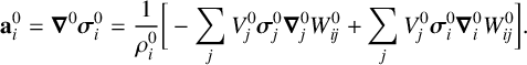 $$ \begin{align} \mathbf{a}_i^0 =\boldsymbol\nabla^0\boldsymbol\sigma^0_i= \frac{1}{\rho^0_i}\bigg[-\sum_jV^0_j\boldsymbol\sigma^0_j\boldsymbol\nabla^0_jW^0_{ij} + \sum_jV^0_j\boldsymbol\sigma^0_i\boldsymbol\nabla^0_iW^0_{ij}\bigg]. \end{align} $$
The first term on the right-hand side of equation (2.5) is the standard SPH approximation for divergence of the stress tensor, while the second term, which is identical to zero, is added to achieve the anti-symmetric property for the momentum conservation. It is noted that the identity $\boldsymbol \nabla ^0_jW^0_{ij}=-\boldsymbol \nabla ^0_iW^0_{ij}$
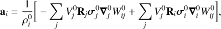
was applied in the second term. Under rotation of particle accelerations back to the current orientation, equation (2.5) is rewritten as
$\boldsymbol \nabla ^0_jW^0_{ij}=-\boldsymbol \nabla ^0_iW^0_{ij}$
was applied in the second term. Under rotation of particle accelerations back to the current orientation, equation (2.5) is rewritten as
 $$ \begin{align} \mathbf{a}_i = \frac{1}{\rho^0_i}\bigg[-\sum_jV^0_j\mathbf{R}_j\boldsymbol\sigma^0_j\boldsymbol\nabla^0_jW^0_{ij} + \sum_jV^0_j\mathbf{R}_i\boldsymbol\sigma^0_i\boldsymbol\nabla^0_iW^0_{ij}\bigg], \end{align} $$
in which $\mathbf {R}_i$
and
$\mathbf {R}_i$
and $\mathbf {R}_j$
are the rotation matrix from the initial orientation to the current orientation of particle i and j, respectively, and will be subsequently discussed.
$\mathbf {R}_j$
are the rotation matrix from the initial orientation to the current orientation of particle i and j, respectively, and will be subsequently discussed.
SPH approximations at boundaries or interfaces, where the support domain of particles is incomplete, basically suffer numerical errors. In the elasticity context, such numerical errors could lead to significantly spurious elastic forces. A renormalization matrix, as defined by Violeau [Reference Violeau35],
 $$ \begin{align*} \mathbf{N}^0_i=\bigg[\sum_jV^0_j\mathbf{r}^0_{ji}\otimes\boldsymbol\nabla^0_iW^0_{ij}\bigg]^{-1}, \end{align*} $$
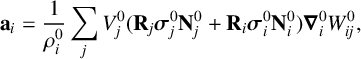
is normally used to correct gradient of the weighted approximation. Accordingly, the corrected gradient of the weight function is written as
 $$ \begin{align*} \boldsymbol\nabla^0_i\tilde{W}^0_{ij}=N^0_i\boldsymbol\nabla^0_iW^0_{ij}. \end{align*} $$
On replacing the gradient of the weight function $\boldsymbol \nabla ^0_iW^0_{ij}$
by its corrected version,
$\boldsymbol \nabla ^0_iW^0_{ij}$
by its corrected version, $\boldsymbol \nabla ^0_i\tilde {W}^0_{ij}$
, equation (2.6) is then rewritten as follows
$\boldsymbol \nabla ^0_i\tilde {W}^0_{ij}$
, equation (2.6) is then rewritten as follows
 $$ \begin{align*} \mathbf{a}_i = \frac{1}{\rho^0_i}\sum_jV^0_j(\mathbf{R}_j\boldsymbol\sigma^0_j\mathbf{N}^0_j+ \mathbf{R}_i\boldsymbol\sigma^0_i\mathbf{N}^0_i)\boldsymbol\nabla^0_iW^0_{ij}, \end{align*} $$
with noting that
 $$ \begin{align*} \boldsymbol\nabla_j^0\tilde{W}^0_{ij}=N^0_j\boldsymbol\nabla_j^0W^0_{ij}=-N^0_j\boldsymbol\nabla^0_iW^0_{ij}. \end{align*} $$
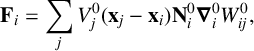
The deformation gradient of particle i is evaluated by
 $$ \begin{align*} \mathbf{F}_i=\sum_jV^0_j(\mathbf{x}_j-\mathbf{x}_i)\mathbf{N}^0_i\boldsymbol\nabla^0_iW^0_{ij}, \end{align*} $$
in which $\mathbf {x}_i$
and
$\mathbf {x}_i$
and $\mathbf {x}_j$
are coordinates of particles i and j in the current deformed object. Strain tensor of particle i is then calculated by
$\mathbf {x}_j$
are coordinates of particles i and j in the current deformed object. Strain tensor of particle i is then calculated by
 $$ \begin{align*} \boldsymbol\epsilon^0_i=\tfrac{1}{2}(\mathbf{F}_i^T\mathbf{F}_i-\mathbf{I}). \end{align*} $$
On using the second Piola–Kirchhoff stress model, the stress of particle i is evaluated as follows:
 $$ \begin{align*} \boldsymbol\sigma^0_i = 2G(\boldsymbol\epsilon^0_i - \tfrac{1}{3}Tr(\boldsymbol\epsilon^0_i)\mathbf{I}) + KTr(\boldsymbol\epsilon^0_i)\mathbf{I}. \end{align*} $$
Rotation matrix $\mathbf {R}$
is extracted from the deformation gradient tensor
$\mathbf {R}$
is extracted from the deformation gradient tensor $\mathbf {F}_i$
. For example, Müller et al. [Reference Müller, Bender, Chentanez, Macklin and Neff23] calculate the rotation matrix
$\mathbf {F}_i$
. For example, Müller et al. [Reference Müller, Bender, Chentanez, Macklin and Neff23] calculate the rotation matrix $\mathbf {R}$
via solving an optimal problem,
$\mathbf {R}$
via solving an optimal problem,
 $$ \begin{align*} \min||\mathbf{R}-\mathbf{A}||^2, \end{align*} $$
in which $||\mathbf {R}-\mathbf {A}||=\sqrt {\sum _i\sum _j(R_{ij}-A_{ij})^2}$
. The optimal rotation matrix can be achieved by adopting the following iteration scheme:
$||\mathbf {R}-\mathbf {A}||=\sqrt {\sum _i\sum _j(R_{ij}-A_{ij})^2}$
. The optimal rotation matrix can be achieved by adopting the following iteration scheme:
 $$ \begin{align*} \mathbf{R}^{k+1} = \mathbf{E(\mathbf{v}^k,\alpha_k)}\mathbf{R}^{k}, \end{align*} $$
in which $\mathbf {E}(\mathbf {v}^k,\alpha _k)$
is a rotation matrix that rotates
$\mathbf {E}(\mathbf {v}^k,\alpha _k)$
is a rotation matrix that rotates $\mathbf {R}^k$
about an axis
$\mathbf {R}^k$
about an axis $\mathbf {v^k}$
an angle
$\mathbf {v^k}$
an angle $\alpha _k$
. The elements of
$\alpha _k$
. The elements of $\mathbf {E}(\mathbf {v}^k,\alpha _k)$
are determined as follows:
$\mathbf {E}(\mathbf {v}^k,\alpha _k)$
are determined as follows:
 $$ \begin{align*} \begin{aligned} E_{11} &= \hat{v}_1^2 + (\hat{v}_2^2 + \hat{v}_3^2)\cos\alpha_k,\\ E_{22} &= \hat{v}_2^2 + (\hat{v}_1^2 + \hat{v}_3^2)\cos\alpha_k,\\ E_{33} &= \hat{v}_3^2 + (\hat{v}_1^2 + \hat{v}_2^2)\cos\alpha_k,\\ E_{12} &= \hat{v}_1\hat{v}_2(1-\cos\alpha_k)-\hat{v}_3\sin\alpha_k,\\ E_{13} &= \hat{v}_1\hat{v}_3(1-\cos\alpha_k)+\hat{v}_2\sin\alpha_k,\\ E_{23} &= \hat{v}_2\hat{v}_3(1-\cos\alpha_k)-\hat{v}_1\sin\alpha_k,\\ E_{21} &= \hat{v}_1\hat{v}_2(1-\cos\alpha_k)+\hat{v}_3\sin\alpha_k,\\ E_{31} &= \hat{v}_1\hat{v}_3(1-\cos\alpha_k)-\hat{v}_2\sin\alpha_k,\\ E_{32} &= \hat{v}_2\hat{v}_3(1-\cos\alpha_k)+\hat{v}_1\sin\alpha_k, \end{aligned} \end{align*} $$
in which $\hat {\mathbf {v}}=(\hat {v}_1,\hat {v}_2,\hat {v}_3)$
is the unit vector of the axis
$\hat {\mathbf {v}}=(\hat {v}_1,\hat {v}_2,\hat {v}_3)$
is the unit vector of the axis $\mathbf {v}^k$
, which is determined from
$\mathbf {v}^k$
, which is determined from
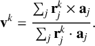 $$ \begin{align*} \mathbf{v}^k=\frac{\sum_j\mathbf{r}^k_j\times\mathbf{a}_j}{\sum_j\mathbf{r}^k_j\cdot\mathbf{a}_j}. \end{align*} $$
The notation $\mathbf {r}^k_j$
and
$\mathbf {r}^k_j$
and $\mathbf {a}_j$
represent column j of
$\mathbf {a}_j$
represent column j of $\mathbf {R}^k$
and
$\mathbf {R}^k$
and $\mathbf {A}$
, respectively. The rotation angle
$\mathbf {A}$
, respectively. The rotation angle $\alpha _k$
is defined by
$\alpha _k$
is defined by $\alpha _k=||\mathbf {v}^k||$
. The iteration scheme can be started with the rotation matrix from the previous time step if the rotating matrix is stored; however, it definitely costs more memory. Another option is using the initial coordinate axes, but it would take more iterating steps to achieve the convergence. Here, we suggest to choose
$\alpha _k=||\mathbf {v}^k||$
. The iteration scheme can be started with the rotation matrix from the previous time step if the rotating matrix is stored; however, it definitely costs more memory. Another option is using the initial coordinate axes, but it would take more iterating steps to achieve the convergence. Here, we suggest to choose $\mathbf {R}^0$
based on the matrix
$\mathbf {R}^0$
based on the matrix $\mathbf {A}$
for a faster convergence as follows:
$\mathbf {A}$
for a faster convergence as follows:
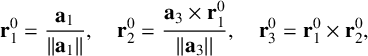 $$ \begin{align*} \mathbf{r}^0_1=\frac{\mathbf{a}_1}{||\mathbf{a}_1||},\quad \mathbf{r}^0_2=\frac{\mathbf{a}_3\times\mathbf{r}^0_1}{||\mathbf{a}_3||},\quad \mathbf{r}^0_3=\mathbf{r}^0_1\times\mathbf{r}^0_2, \end{align*} $$
in which $\mathbf {r}^0_i$
is column i of
$\mathbf {r}^0_i$
is column i of $\mathbf {R}^0$
.
$\mathbf {R}^0$
.
2.4 Equation of state
Pressure arising in a deformed elastic structure is calculated from trace of the of the stress tensor,
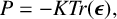 $$ \begin{align} P=-KTr(\boldsymbol\epsilon), \end{align} $$
in which K is the bulk modulus of the material and $\boldsymbol \epsilon $
is the strain tensor. It is assumed that an elastic object with dimension of
$\boldsymbol \epsilon $
is the strain tensor. It is assumed that an elastic object with dimension of $(L_1,L_2,L_3)$
is stretched by a displacement vector
$(L_1,L_2,L_3)$
is stretched by a displacement vector $\mathbf {u} = (u_1,u_2,u_3)$
. A trace of the strain tensor can be rewritten as
$\mathbf {u} = (u_1,u_2,u_3)$
. A trace of the strain tensor can be rewritten as
 $$ \begin{align} Tr(\boldsymbol\epsilon) = \epsilon_{11} + \epsilon_{22} + \epsilon_{33} = \frac{u_1}{L_1} + \frac{u_2}{L_2} + \frac{u_3}{L_3}. \end{align} $$
However, the ratio of the nondeformed volume ( $V_0$
) and the deformed volume (V) is evaluated by
$V_0$
) and the deformed volume (V) is evaluated by
 $$ \begin{align} \frac{V_0}{V}&=\frac{L_1L_2L_3}{(L_1+u_1)(L_2+u_2)(L_3+u_3)} \nonumber\\ &=\frac{1}{(1+u_1/L_1)(1+u_2/L_2)(1+u_3/L_3)}\nonumber\\ &\approx1-\bigg(\frac{u_1}{L_1}+\frac{u_2}{L_2}+\frac{u_3}{L_3}\bigg)\nonumber\\ &= 1-(\epsilon_{11} + \epsilon_{22} + \epsilon_{33}), \end{align} $$
for $u_i<<L_i$
, or
$u_i<<L_i$
, or $\epsilon _{ii}<<1$
, that is, small strains. On using the relation
$\epsilon _{ii}<<1$
, that is, small strains. On using the relation
 $$ \begin{align} \frac{\rho}{\rho_0} = \frac{V_0}{V} \end{align} $$
and equations (2.7)–(2.10), equation (2.7) can be rewritten as follows:
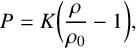 $$ \begin{align} P = K\bigg(\frac{\rho}{\rho_0}-1\bigg), \end{align} $$
which has the form of a state equation $P=P_0(\rho /\rho _0-1)$
, in which
$P=P_0(\rho /\rho _0-1)$
, in which $P_0$
equals to the bulk modulus of the material.
$P_0$
equals to the bulk modulus of the material.
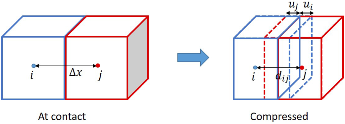
Demonstration for an elastic collision of two SPH particles.
2.5 Contact-force model for elastic collisions
As two elastic objects collide, they are locally deformed and local pressure will arise to pull the objects apart as a consequence. In SPH, we can model the repulsive force between two colliding objects as a sum of pair-wise repulsive forces between their component particles, as illustrated in Figure 1. Assuming that the distance of two particles at contact equals to the initial particle gap ( $\triangle x$
) and their distance after the collision is
$\triangle x$
) and their distance after the collision is $d_{ij}<\triangle x$
, the magnitude of the elastic force acting on each particle is equal to the pressure P, arising due to the compression, multiplied by the contact area A,
$d_{ij}<\triangle x$
, the magnitude of the elastic force acting on each particle is equal to the pressure P, arising due to the compression, multiplied by the contact area A,
 $$ \begin{align} F_r = AP. \end{align} $$
On applying the equation of state (2.11) for P and substituting $A=\triangle x^{n-1}$
(n is the dimension number), equation (2.12) can be rewritten as
$A=\triangle x^{n-1}$
(n is the dimension number), equation (2.12) can be rewritten as
 $$ \begin{align*} F_r = \triangle x^{n-1}K\bigg(\frac{\rho}{\rho_0}-1\bigg). \end{align*} $$
For particle i,
 $$ \begin{align*} F_r = \triangle x^{n-1}K_1\bigg(\frac{\rho_i}{\rho_{i,0}}-1\bigg)\approx\triangle x^{n-2}K_1u_i, \end{align*} $$
and for particle j,
 $$ \begin{align*} F_r \approx \triangle x^{n-2}K_2u_j \end{align*} $$
with noting that $u_i$
and
$u_i$
and $u_j$
are the compressing displacement of particle i and j. For the generality,
$u_j$
are the compressing displacement of particle i and j. For the generality, $K_1$
and
$K_1$
and $K_2$
are assumed different, and therefore
$K_2$
are assumed different, and therefore $u_i\ne u_j$
. Since
$u_i\ne u_j$
. Since $u_i+u_j=\triangle x- d_{ij}$
, which is the total displacement,
$u_i+u_j=\triangle x- d_{ij}$
, which is the total displacement,
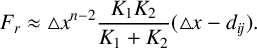 $$ \begin{align} F_r \approx \triangle x^{n-2}\frac{K_1K_2}{K_1+K_2}(\triangle x- d_{ij}). \end{align} $$
Equation (2.13) has the form of Hooke’s law with the spring coefficient defined by
 $$ \begin{align*} k=\triangle x^{n-2}\frac{K_1K_2}{K_1+K_2}. \end{align*} $$
If $K_1=K_2=K$
, that is, the colliding objects have the same bulk modulus, the spring coefficient is reduced as
$K_1=K_2=K$
, that is, the colliding objects have the same bulk modulus, the spring coefficient is reduced as $k=\triangle x^{n-2}K/2$
. Then, the interacting force acting on particle i by particle j and vice versa are written as
$k=\triangle x^{n-2}K/2$
. Then, the interacting force acting on particle i by particle j and vice versa are written as
 $$ \begin{align} \mathbf{F}^{j\rightarrow i}_r &= F_r\mathbf{e}_{ij}, \end{align} $$
 $$ \begin{align} \mathbf{F}^{i\rightarrow j}_r &= F_r\mathbf{e}_{ji}. \end{align} $$
3 Numerical results
In this section, we present some numerical experiments for typical elastic problems, including beam bending, truss extension and compression, and two-rings collision in which the objects experience large deformations. For convenience in discussions, the Eulerian algorithm developed by Monaghan [Reference Gray, Monaghan and Swift11, Reference Monaghan21] based on the current particle configuration without and with the artificial stresses is called current configuration based SPH (CCB-SPH) and current configuration based with artificial tension SPH (CCBWAT-SPH), respectively, and the Lagrangian SPH algorithm of Tran-Duc et al. [Reference Tran-Duc, Meylan and Thamwattana32] based on the initial configuration is called ICB-SPH.
3.1 Bending of a cantilever beam
The cantilevered beam is a common engineering structure that has one end fixed or supported and the other end free. On application of a vertically point-load at its free end, the beam is bent. Upon the bending, the upper side of the beam is stretched and the lower side is compressed. The beam-bending problem is simulated by adopting the three SPH schemes. In the simulations, the beam has a length of $L=0.2$
m, a thickness of
$L=0.2$
m, a thickness of $H=2$
cm and Young’s modulus of
$H=2$
cm and Young’s modulus of $E=20$
GPa; a vertical force
$E=20$
GPa; a vertical force $F_y=-250$
N is applied downward at the free end and a particle gap
$F_y=-250$
N is applied downward at the free end and a particle gap $\triangle x=2$
mm is used in all the subsequent simulations.
$\triangle x=2$
mm is used in all the subsequent simulations.
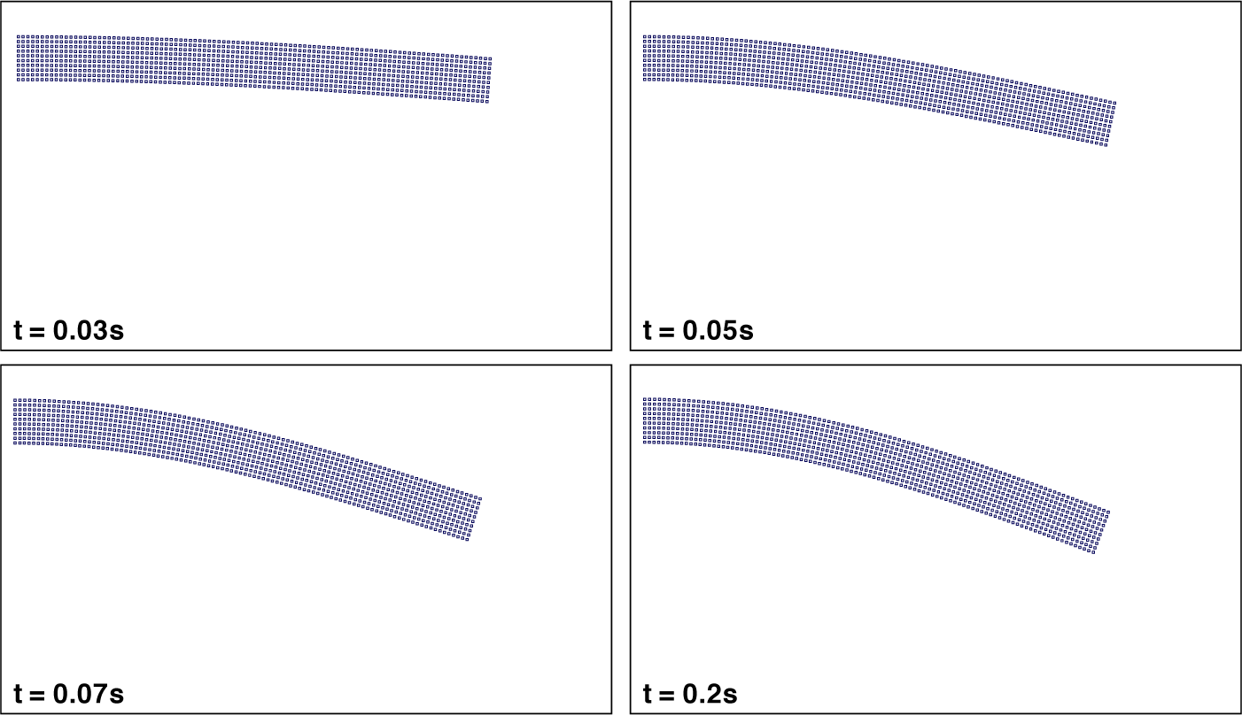
Figure 2 shows some snapshots of the beam’s deformation simulated with the CCB-SPH scheme at different points of time, $t=0.03$
s,
$t=0.03$
s, $0.05$
s,
$0.05$
s, $0.07$
s and
$0.07$
s and $0.08$
s. Upon the tension occurring in the upper region of the beam, the gap between particles is enlarged. At
$0.08$
s. Upon the tension occurring in the upper region of the beam, the gap between particles is enlarged. At $t=0.05$
s, particles’ gap near the fixed end where the curvature is high becomes significantly large compared to the initial particle gap. As a consequence, the particle distribution in that region becomes uneven. The nonuniformity becomes worse and worse until a small crack emerges shortly in the weakest region at
$t=0.05$
s, particles’ gap near the fixed end where the curvature is high becomes significantly large compared to the initial particle gap. As a consequence, the particle distribution in that region becomes uneven. The nonuniformity becomes worse and worse until a small crack emerges shortly in the weakest region at $t=0.07$
s, as observed in Figure 2. The crack continues enlarging, the beam fails to resist the load and then it breaks into two parts.
$t=0.07$
s, as observed in Figure 2. The crack continues enlarging, the beam fails to resist the load and then it breaks into two parts.
Bending of a cantilever beam simulated using the CCB-SPH algorithm. The beam has length $L=0.2$
m, thickness
$L=0.2$
m, thickness $H=2$
cm and Young’s modulus
$H=2$
cm and Young’s modulus $E=20$
GPa. A vertical load
$E=20$
GPa. A vertical load $F_y=-250$
N is applied downward at its free end.
$F_y=-250$
N is applied downward at its free end.

The emergence of uneven particle configurations near the fixed end caused the failure of the beam as simulated with CCB-SPH. Theoretically, as the gap between one SPH particle and its nearest neighbouring particles is stretched exceeding a certain value, the value of the weight-function derivative rapidly drops due to the bell-shaped form of the weight function. Simultaneously, the elastic stress gets larger due to a larger deformation gradient. As seen in equation (2.3), the interacting forces between two neighbouring particles are proportional to the product of elastic stress and the value of the weight-function derivative. Therefore, a substantial drop in the value of the weight-function derivative could decrease the interacting forces between two particles that are supposed to increase under the high stretch deformation. Consequently, the beam strength is weakened locally. Another reason for the failure is that the uneven particle configuration leads to an imbalance in the interacting forces between the two sides of a stretched particle. The higher stretched side has a smaller contribution in equation (2.3) in comparison to the opposite side.
The simulation is re-run using the CCBWAT-SPH algorithm, in which the artificial stresses are switched on. The values of the parameters of the artificial stress terms are chosen as $a=1$
,
$a=1$
, $\epsilon =0.3$
and
$\epsilon =0.3$
and $n=6$
. As observed in Figure 3, no cracks are seen in the deformed beam with the inclusion of the artificial stresses. Particle configuration in the highly stretched region near the fixed end is also seen to be more even than that in the previous simulation with CCB-SPH. The beam can withstand the applied load and reaches the equilibrium state. It can be said that the artificial stresses are successful in maintaining the particle uniformity and hence the beam strength. As the particle configuration in the upper region is stretched by the beam bending, the artificial tensile stress
$n=6$
. As observed in Figure 3, no cracks are seen in the deformed beam with the inclusion of the artificial stresses. Particle configuration in the highly stretched region near the fixed end is also seen to be more even than that in the previous simulation with CCB-SPH. The beam can withstand the applied load and reaches the equilibrium state. It can be said that the artificial stresses are successful in maintaining the particle uniformity and hence the beam strength. As the particle configuration in the upper region is stretched by the beam bending, the artificial tensile stress $\mathbf {T}_{ij}$
will arise to partly compensate for the underestimation of the elastic forces in the stretched region. It is noted that the added stress term
$\mathbf {T}_{ij}$
will arise to partly compensate for the underestimation of the elastic forces in the stretched region. It is noted that the added stress term $\Pi _{ij}$
does not directly suppress the tensile instability but only stabilizes the system by damping spurious fluctuations in the pressure field.
$\Pi _{ij}$
does not directly suppress the tensile instability but only stabilizes the system by damping spurious fluctuations in the pressure field.
Bending of a cantilever beam simulated using the CCBWAT-SPH algorithm. The beam has length $L=0.2$
m, thickness
$L=0.2$
m, thickness $H=2$
cm and Young’s modulus
$H=2$
cm and Young’s modulus $E=20$
GPa. A vertical load
$E=20$
GPa. A vertical load $F_y=-250$
N is applied downward at its free end. The values of the parameters of the artificial stress terms are
$F_y=-250$
N is applied downward at its free end. The values of the parameters of the artificial stress terms are $a=1$
,
$a=1$
, $\epsilon =0.3$
and
$\epsilon =0.3$
and $n=6$
.
$n=6$
.

The beam bending is again simulated using the ICB-SPH algorithm, and collective snapshots of the beam deformation are shown in Figure 4. Unlike the CCB-SPH scheme, the beam simulated with ICB-SPH responds very well to the load, and no failures/cracks are observed during the beam motion. The particle distribution is also seen to be uniformly stretched in the highly tensile region, and no uneven particle configurations are observed. The beam reaches the equilibrium state then. Since, in the ICB-SPH scheme, the differential operators, such as divergence and gradient, are defined on the initial configuration which is initially generated uniformly, the ICB-SPH algorithm does not experience any numerical issues related to the deformed particle configuration as in the CCB-SPH.
Bending of a cantilever beam simulated using the ICB-SPH algorithm. The beam has length $L=0.2$
m, thickness
$L=0.2$
m, thickness $H=2$
cm and Young’s modulus
$H=2$
cm and Young’s modulus $E=20$
GPa. A vertical load
$E=20$
GPa. A vertical load $F_y=-250$
N is applied downward at its free end.
$F_y=-250$
N is applied downward at its free end.
As observed in Figures 3 and 4, there is a little difference in the deflection of the beam in the equilibrium state when simulating with the CCBWAT-SPH and ICB-SPH algorithms. More specifically, the beam is bent more with the CCBWAT-SPH algorithm than with the ICB-SPH algorithm. So, a concern about which scheme produces a correct maximum deflection of the beam naturally arises. Hence, a theory for finite deflections of a cantilever beam for the verification purpose is used. Accordingly, based on the moment balance, the bending equation of a uniform cross-section beam can be written as follows [Reference Wang, Chena and Liao36]:
 $$ \begin{align*} \frac{d\theta^2}{d^2\zeta}+\alpha\cos\theta = 0, \quad 0< \zeta < 1, \end{align*} $$
in which $\theta $
is the rotational angle of the cross-section along the beam axis,
$\theta $
is the rotational angle of the cross-section along the beam axis, $\zeta =s/L$
is dimensionless longitudinal coordinate and
$\zeta =s/L$
is dimensionless longitudinal coordinate and $\alpha =F_yL^2/EI$
. Here, s is the longitudinal coordinate along the deformed beam, L is the initial beam length,
$\alpha =F_yL^2/EI$
. Here, s is the longitudinal coordinate along the deformed beam, L is the initial beam length, $I=LH^3/12$
is the moment of inertia of the beam with thickness of H and E is Young’s modulus. Boundary conditions at the fixed and free ends are
$I=LH^3/12$
is the moment of inertia of the beam with thickness of H and E is Young’s modulus. Boundary conditions at the fixed and free ends are $\theta (0)=0$
and
$\theta (0)=0$
and ${(d\theta )/(d\zeta )(1)=0}$
, respectively. Maximum vertical (
${(d\theta )/(d\zeta )(1)=0}$
, respectively. Maximum vertical ( $\delta _h$
) and horizontal (
$\delta _h$
) and horizontal ( $\delta _v$
) displacements in the equilibrium state of the beam are evaluated by
$\delta _v$
) displacements in the equilibrium state of the beam are evaluated by
 $$ \begin{align} \delta_v&=L\bigg[1-\frac{2}{\sqrt{\alpha}}(E(\mu)-E(\varphi,\mu))\bigg], \end{align} $$
 $$ \begin{align} \delta_h&=L\bigg(1-\sqrt{\frac{2\sin\theta_B}{\alpha}}\bigg),\!\qquad\qquad \end{align} $$
in which
 $$ \begin{align*}E(\mu)=\int_0^{\pi/2}\sqrt{1-\mu^2\sin^2x}\,dx\quad \text{and} \quad E(\varphi,\mu)=\int_0^{\varphi}\sqrt{1-\mu^2\sin^2x}\,dx\end{align*} $$
are the complete and incomplete integrals of the second kind, respectively, with ${\mu =\sqrt {(1+\sin \theta _B)/2}}$
and
${\mu =\sqrt {(1+\sin \theta _B)/2}}$
and $\varphi =\arcsin {(1/\sqrt {2}\mu )}$
. The two functions can be readily evaluated using computing packages, such as Matlab or Maple. An asymptotic solution for the slope at the free end (
$\varphi =\arcsin {(1/\sqrt {2}\mu )}$
. The two functions can be readily evaluated using computing packages, such as Matlab or Maple. An asymptotic solution for the slope at the free end ( $\theta _B$
), for
$\theta _B$
), for $0<\alpha <1.5$
, is written as follows [Reference Wang, Chena and Liao36]:
$0<\alpha <1.5$
, is written as follows [Reference Wang, Chena and Liao36]:
 $$ \begin{align} \theta_B &= 0.5\alpha-4.56543\times10^{-2}\alpha^3+8.02901\times10^{-3}\alpha^5 \nonumber \\ &\quad -8.59983\times10^{-4}\alpha^7+2.28499\times10^{-6}\alpha^{9}. \end{align} $$
For an infinitesimal deflection ( $\alpha <<1$
),
$\alpha <<1$
), $\delta _h\approx 0$
,
$\delta _h\approx 0$
, $\delta _v=L\alpha /3$
and
$\delta _v=L\alpha /3$
and $\theta _B=0.5\alpha $
, which are similar to the evaluations using the linear theory. Once the bending angle at the free end,
$\theta _B=0.5\alpha $
, which are similar to the evaluations using the linear theory. Once the bending angle at the free end, $\theta _B$
, is known, the vertical and horizontal displacements can be evaluated using equations (3.1) and (3.2).
$\theta _B$
, is known, the vertical and horizontal displacements can be evaluated using equations (3.1) and (3.2).
In the investigated case above, the value of $\alpha $
is
$\alpha $
is $0.75$
. On using equation (3.3),
$0.75$
. On using equation (3.3), $\theta _B$
is approximately
$\theta _B$
is approximately $0.358$
, or
$0.358$
, or $20.5^\circ $
. Then, substituting
$20.5^\circ $
. Then, substituting $\theta _B=0.358$
into equations (3.1) and (3.2) yields the maximum displacements of the beam,
$\theta _B=0.358$
into equations (3.1) and (3.2) yields the maximum displacements of the beam, $(\delta _h,\delta _v)$
= (
$(\delta _h,\delta _v)$
= ( $-6.792$
mm,
$-6.792$
mm, $-47.12$
mm). Those values in the CCBWAT-SPH and ICB-SPH simulations are (
$-47.12$
mm). Those values in the CCBWAT-SPH and ICB-SPH simulations are ( $-9.541$
mm,
$-9.541$
mm, $-58.62$
mm) and (
$-58.62$
mm) and ( $-7.096$
mm,
$-7.096$
mm, $-47.66$
mm), respectively. It can be seen that the displacements obtained from the ICB-SPH simulation are very close to the theoretical values, while the beam’s deflections obtained from the CCBWAT-SPH simulation are larger than the theoretical values in magnitude. In other words, the beam is bent more with the CCBWAT-SPH. This result also shows that although the artificial stresses terms successfully prevent the beam from cracking, they do not completely remove the tensile effect that weakens the beam, at least for the chosen values of the parameters of the artificial stresses. It is crucial to comment that calibrations for the stresses’ parameters in the CCBWAT-SPH scheme need to be done carefully for every specific problem. Its adverse effects are nontrivial to characterize.
$-47.66$
mm), respectively. It can be seen that the displacements obtained from the ICB-SPH simulation are very close to the theoretical values, while the beam’s deflections obtained from the CCBWAT-SPH simulation are larger than the theoretical values in magnitude. In other words, the beam is bent more with the CCBWAT-SPH. This result also shows that although the artificial stresses terms successfully prevent the beam from cracking, they do not completely remove the tensile effect that weakens the beam, at least for the chosen values of the parameters of the artificial stresses. It is crucial to comment that calibrations for the stresses’ parameters in the CCBWAT-SPH scheme need to be done carefully for every specific problem. Its adverse effects are nontrivial to characterize.
For a thorough comparison of the performance of the three SPH schemes, simulations in various load scenarios, $F_y$
ranging from
$F_y$
ranging from $-10$
N to
$-10$
N to $-150$
N, are carried out, and the maximum beam’s displacements are then summarized in Table 1. With the CCB-SPH scheme, the beam cannot withstand the applied load in most simulated cases except
$-150$
N, are carried out, and the maximum beam’s displacements are then summarized in Table 1. With the CCB-SPH scheme, the beam cannot withstand the applied load in most simulated cases except $-10$
N and
$-10$
N and $-25$
N. In the two cases, the vertical displacement of the beam is approximately
$-25$
N. In the two cases, the vertical displacement of the beam is approximately $19.5\%$
and
$19.5\%$
and $66.4\%$
, respectively, larger than the theoretical values. With the CCBWAT-SPH, the beam responds well in all the simulated cases. Compared with the theoretical values, the vertical displacement obtained with the CCBWAT-SPH is approximately 20%–25% larger. The vertical displacements obtained from the ICB-SPH are a few percent different from the theoretical values, as listed in Table 2.
$66.4\%$
, respectively, larger than the theoretical values. With the CCBWAT-SPH, the beam responds well in all the simulated cases. Compared with the theoretical values, the vertical displacement obtained with the CCBWAT-SPH is approximately 20%–25% larger. The vertical displacements obtained from the ICB-SPH are a few percent different from the theoretical values, as listed in Table 2.
Vertical and horizontal deflections of a bent cantilever beam ( $L=0.2$
m,
$L=0.2$
m, $H=2$
cm and
$H=2$
cm and ${E=20}$
GPa) under various load scenarios, from
${E=20}$
GPa) under various load scenarios, from $-10$
N to
$-10$
N to $-250$
N. The values are obtained from simulations adopting the CCB-SPH, CCBWAT-SPH and ICB-SPH algorithms, and the theoretical model, equations (3.1)–(3.3), for a beam with finite deflections.
$-250$
N. The values are obtained from simulations adopting the CCB-SPH, CCBWAT-SPH and ICB-SPH algorithms, and the theoretical model, equations (3.1)–(3.3), for a beam with finite deflections.

Numerical convergence for various spatial resolutions ( $\triangle x$
) for the case of cantilever beam bending. The relative errors compared with their corresponding theoretical values for the horizontal (
$\triangle x$
) for the case of cantilever beam bending. The relative errors compared with their corresponding theoretical values for the horizontal ( $\delta _h$
) and vertical (
$\delta _h$
) and vertical ( $\delta _v$
) displacements of the free end are shown for the spatial resolution varied from
$\delta _v$
) displacements of the free end are shown for the spatial resolution varied from $5$
mm down to
$5$
mm down to $0.5$
mm.
$0.5$
mm.

Convergence rate of the ICB-SPH algorithm with respect to the spatial resolution is demonstrated via simulations for $F_y=-75$
N,
$F_y=-75$
N, $-150$
N and
$-150$
N and $-250$
N. The simulations are carried out for different particle sizes from
$-250$
N. The simulations are carried out for different particle sizes from $\triangle x=5$
mm down to
$\triangle x=5$
mm down to $0.5$
mm. As summarized in Table 2, the numerical convergence is achieved for the particle size less than or equal
$0.5$
mm. As summarized in Table 2, the numerical convergence is achieved for the particle size less than or equal $0.5$
mm with the relative error to their corresponding theoretical values less than
$0.5$
mm with the relative error to their corresponding theoretical values less than $0.2$
% in all the investigated cases.
$0.2$
% in all the investigated cases.
3.2 Truss extension and compression
In the previous section, the cantilever beam underwent bending deformation by applying a vertical load at its free end. Upon the bending, the beam experienced both compression and tension at the same time-stretch along the top surface and compression along the bottom surface. Tensile instability occurred in the top surface region near the fixed end, causing the failure of the beam. There is a concern that the compression in the bottom region could have played a role in the failure. It is known that as SPH particles come close together at distances much less than the initial particle gap, known as particle clumping, interacting forces between them also decreases, because $\partial W(r,h)/\partial r\rightarrow 0$
as
$\partial W(r,h)/\partial r\rightarrow 0$
as $r\rightarrow 0$
. This is another issue in SPH which arises from the bell shape of the weight function. So, we now separately investigate a beam under pure compression and pure tension occurring along its longitudinal axis. A horizontal force
$r\rightarrow 0$
. This is another issue in SPH which arises from the bell shape of the weight function. So, we now separately investigate a beam under pure compression and pure tension occurring along its longitudinal axis. A horizontal force $F_x$
is applied to its free end to generate a pure compression or a pure tension. If
$F_x$
is applied to its free end to generate a pure compression or a pure tension. If $F_x>0$
, the beam is stretched, and vice versa. The beam has a length of
$F_x>0$
, the beam is stretched, and vice versa. The beam has a length of $L=0.2$
m, a thickness of
$L=0.2$
m, a thickness of $H=5$
cm and Young’s modulus of
$H=5$
cm and Young’s modulus of $E=2$
GPa. The beam simulated in this section has a larger aspect ratio than that in the previous section to avoid buckling instability that would occur under high compression. Again, the simulations will be carried out using the three SPH schemes in various load scenarios for comparison. The particle size of
$E=2$
GPa. The beam simulated in this section has a larger aspect ratio than that in the previous section to avoid buckling instability that would occur under high compression. Again, the simulations will be carried out using the three SPH schemes in various load scenarios for comparison. The particle size of $2$
mm is used again.
$2$
mm is used again.
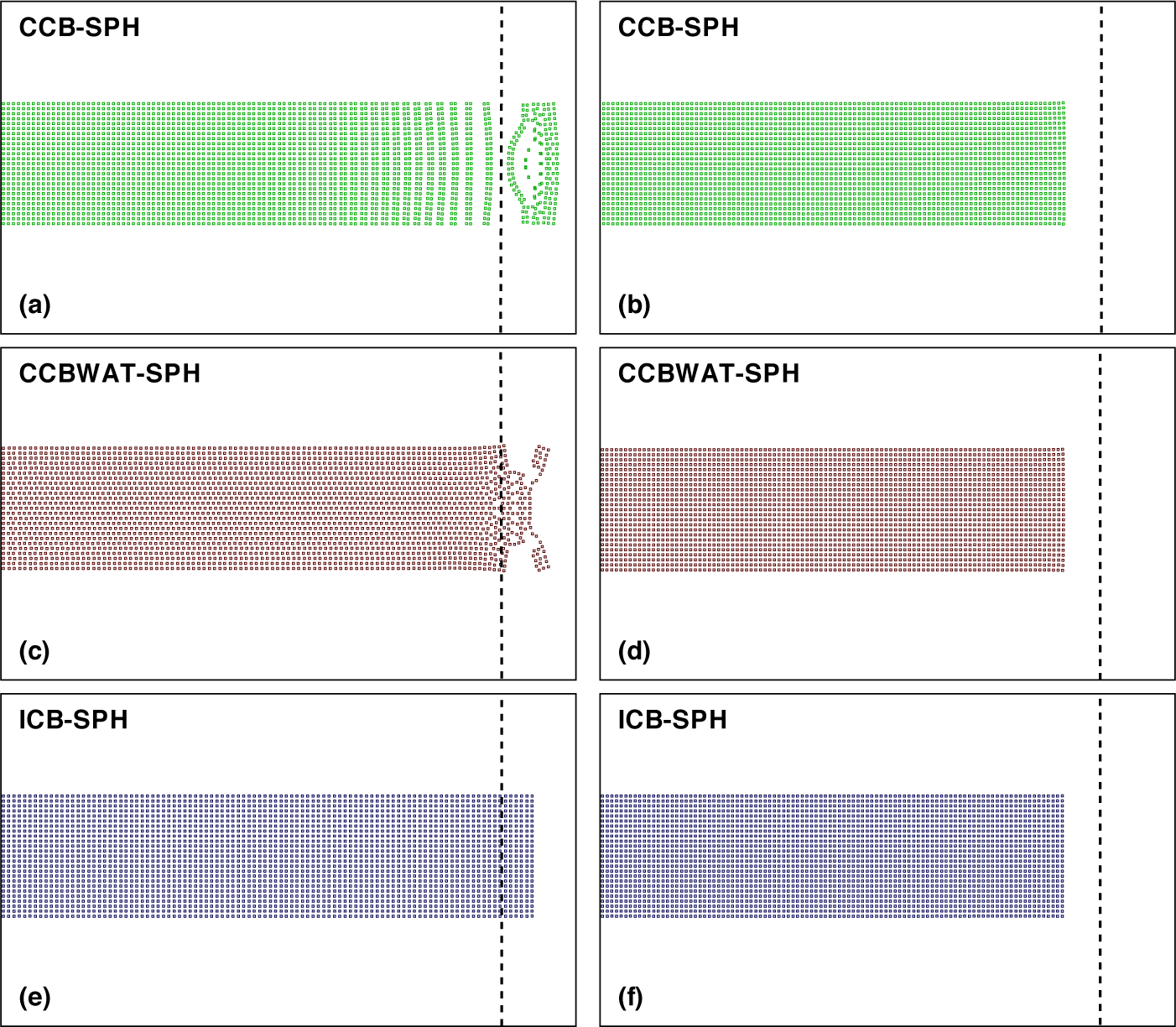
Figure 5 shows deformations of the beam under a compressive load ${F_x=-3000}$
N and a tensile load
${F_x=-3000}$
N and a tensile load $F_x=3000$
N. It can be seen that the beam simulated with the CCB-SPH scheme is broken under the tension, but it responds well to the compressive load (Figures 5(a) and 5(b)). In the compression case, the beam’s displacement is
$F_x=3000$
N. It can be seen that the beam simulated with the CCB-SPH scheme is broken under the tension, but it responds well to the compressive load (Figures 5(a) and 5(b)). In the compression case, the beam’s displacement is $-6.02$
mm, corresponding to the strain in the x-direction of
$-6.02$
mm, corresponding to the strain in the x-direction of $\varepsilon =-6.02/20=-0.301$
. Theoretically, normal stress in the x-direction can be evaluated by
$\varepsilon =-6.02/20=-0.301$
. Theoretically, normal stress in the x-direction can be evaluated by
 $$ \begin{align*} \sigma^{xx} = \frac{F_x}{A}, \end{align*} $$
in which A is the cross-sectional area of the beam. Then, displacement of the free end along the x-direction is calculated as
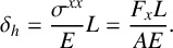 $$ \begin{align} \delta_h=\frac{\sigma^{xx}}{E}L= \frac{F_xL}{AE}. \end{align} $$
So, $\delta _h=-6$
mm in this case. It can be seen that the value obtained from the CB-SPH scheme is very close to the theoretical value in the compression case.
$\delta _h=-6$
mm in this case. It can be seen that the value obtained from the CB-SPH scheme is very close to the theoretical value in the compression case.
Stretch deformation of the cantilever beam ( $L=0.2$
m,
$L=0.2$
m, $H=5$
cm and
$H=5$
cm and $E=2$
GPa) under an axial force
$E=2$
GPa) under an axial force $F=3000$
N simulated using the CCB-SPH, CCBWAT-SPH and ICB-SPH algorithms.
$F=3000$
N simulated using the CCB-SPH, CCBWAT-SPH and ICB-SPH algorithms.

The beam simulated with the CCBWAT-SPH scheme responds well to both the tensile and compressive loads, as observed in Figures 5(c) and 5(d). The beam displacement is $7.15$
mm and
$7.15$
mm and $-6.03$
mm in the tension and compression simulations, respectively. Compared with the theoretical value, the displacement in the tension case is approximately
$-6.03$
mm in the tension and compression simulations, respectively. Compared with the theoretical value, the displacement in the tension case is approximately $20\%$
higher, while the displacement in the compression simulation is very consistent. For the simulations using the ICB-SPH (Figures 5(e) and 5(f)), the beam’s displacements are
$20\%$
higher, while the displacement in the compression simulation is very consistent. For the simulations using the ICB-SPH (Figures 5(e) and 5(f)), the beam’s displacements are $5.82$
mm and
$5.82$
mm and $-5.95$
mm, respectively, which are very close to the theoretical values.
$-5.95$
mm, respectively, which are very close to the theoretical values.
The magnitude of the applied forces is increased to $7000$
N. As observed in Figure 6, the three schemes work well in the compression simulations, and the displacement obtained from the simulations agrees with the theoretical value, as seen in Table 3. However, only the beam simulated with ICB-SPH responds well to the tensile load, and the beam is broken in the other two simulations with the CCB-SPH and CCBWAT-SPH schemes. Two more numerical experiments with the magnitude of the applied force of
$7000$
N. As observed in Figure 6, the three schemes work well in the compression simulations, and the displacement obtained from the simulations agrees with the theoretical value, as seen in Table 3. However, only the beam simulated with ICB-SPH responds well to the tensile load, and the beam is broken in the other two simulations with the CCB-SPH and CCBWAT-SPH schemes. Two more numerical experiments with the magnitude of the applied force of $1000$
N and
$1000$
N and $5000$
N are also carried out, and the beam’s displacements are summarized in Table 3 for the comparison. In the investigated cases, the numerical convergence is again achieved for the particle size, or the spatial resolution, less than or equal to
$5000$
N are also carried out, and the beam’s displacements are summarized in Table 3 for the comparison. In the investigated cases, the numerical convergence is again achieved for the particle size, or the spatial resolution, less than or equal to $0.5$
mm, as shown in Table 4.
$0.5$
mm, as shown in Table 4.
Stretch deformation of the cantilever beam ( $L=0.2$
m,
$L=0.2$
m, $H=5$
cm and
$H=5$
cm and $E=2$
GPa) under an axial force
$E=2$
GPa) under an axial force $F=7000$
N simulated using the CCB-SPH, CCBWAT-SPh and ICB-SPH algorithms.
$F=7000$
N simulated using the CCB-SPH, CCBWAT-SPh and ICB-SPH algorithms.
Horizontal displacement of the cantilever beam ( $L=0.2$
m,
$L=0.2$
m, $H=5$
cm and
$H=5$
cm and $E=2$
GPa) under various tension/compression scenarios in comparison to the theoretical values obtained using equation (3.4). The simulations adopt the CCB-SPH, CCBWAT-SPH and ICB-SPH algorithms.
$E=2$
GPa) under various tension/compression scenarios in comparison to the theoretical values obtained using equation (3.4). The simulations adopt the CCB-SPH, CCBWAT-SPH and ICB-SPH algorithms.

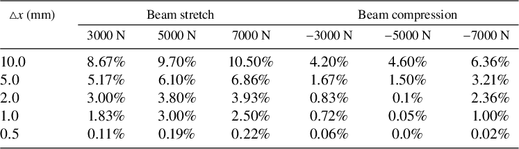
Numerical convergence for various spatial resolutions ( $\triangle x$
) for the beam pure stretch and compression. The relative errors compared with their corresponding theoretical values for the horizontal displacement (
$\triangle x$
) for the beam pure stretch and compression. The relative errors compared with their corresponding theoretical values for the horizontal displacement ( $\delta _h$
) at the free end are presented for the spatial resolution varied from
$\delta _h$
) at the free end are presented for the spatial resolution varied from $10$
mm down to
$10$
mm down to $0.5$
mm.
$0.5$
mm.
In conclusion, the three SPH schemes work very well under the compressive loads, but only the ICB-SPH can withstand all the applied tensile loads, and the beam’s displacements are very consistent with the theoretical values. The CCB-SPH scheme fails to tackle the tensile deformation in all the investigated cases, while the CCBWAT-SPH only works well for the tensile loads up to $3000$
N.
$3000$
N.
3.3 Collision of two elastic rings
Elastic collision of two moving rings is another common testing problem for the tensile instability occurring in elastic interactions with SPH [Reference Gray, Monaghan and Swift11, Reference Monaghan21, Reference Swegle, Hicks and Attaway30]. In this section, the problem is again simulated using the three SPH schemes. Two circular rings have the same diameter of $0.2$
m, a thickness of
$0.2$
m, a thickness of $1$
cm, Young’s modulus of
$1$
cm, Young’s modulus of $E=20$
GPa and move at the same constant velocity
$E=20$
GPa and move at the same constant velocity $V_r$
but in opposite directions. Upon the collision, one ring exerts forces onto the other and vice versa that causes elastic deformations in the two rings. As the stored elastic energy (from the elastic deformations) in the rings overcomes their kinetic energy, they will be repulsed back. Here, the contact force between the rings is modelled as a sum of pair-wise contact force between their component particles, as presented in Section 2.5. Accordingly, two SPH particles belonging to the two rings are assumed to interact with each other as their distance less than the initial particle gap
$V_r$
but in opposite directions. Upon the collision, one ring exerts forces onto the other and vice versa that causes elastic deformations in the two rings. As the stored elastic energy (from the elastic deformations) in the rings overcomes their kinetic energy, they will be repulsed back. Here, the contact force between the rings is modelled as a sum of pair-wise contact force between their component particles, as presented in Section 2.5. Accordingly, two SPH particles belonging to the two rings are assumed to interact with each other as their distance less than the initial particle gap $\triangle x$
and their interacting forces are evaluated using equations (2.14) and (2.15).
$\triangle x$
and their interacting forces are evaluated using equations (2.14) and (2.15).
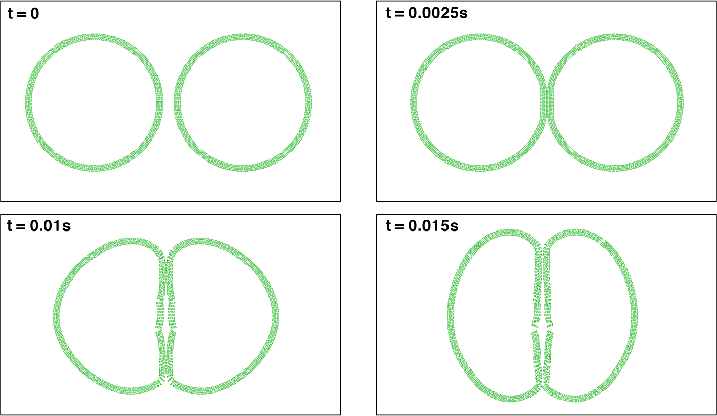
First, it is assumed that $V_r=5$
m/s. Figure 7 displays some snapshots during the rings’ collision simulated with the CCB-SPH scheme. It can be seen that cracks quickly appear along the contact region of the two rings, where the deformations are substantial, at
$V_r=5$
m/s. Figure 7 displays some snapshots during the rings’ collision simulated with the CCB-SPH scheme. It can be seen that cracks quickly appear along the contact region of the two rings, where the deformations are substantial, at $t=0.01$
s. The contact region of each ring is subsequently seen broken into pieces after
$t=0.01$
s. The contact region of each ring is subsequently seen broken into pieces after $0.02$
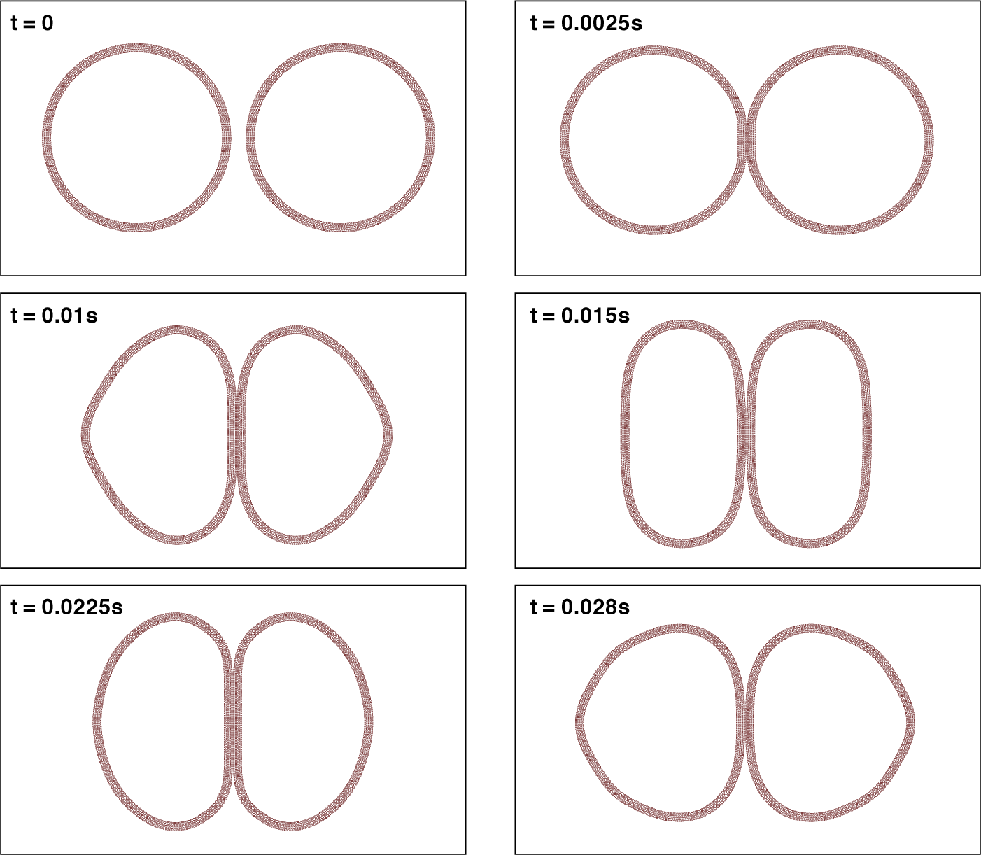
s. This phenomenon is not observed in the simulations using the CCBWAT-SPH scheme and the ICB-SPH scheme, as observed in Figures 8 and 9. Again, we can see a remarkable difference in dynamical responses of the two rings as simulated with the CCBWAT-SPH and the ICB-SPH algorithms. The added tensile and viscous stresses seem to have altered the material properties of the ring somehow in an unexpected and predicted way.
$0.02$
s. This phenomenon is not observed in the simulations using the CCBWAT-SPH scheme and the ICB-SPH scheme, as observed in Figures 8 and 9. Again, we can see a remarkable difference in dynamical responses of the two rings as simulated with the CCBWAT-SPH and the ICB-SPH algorithms. The added tensile and viscous stresses seem to have altered the material properties of the ring somehow in an unexpected and predicted way.
Collision of two elastic rings, each of which has a similar diameter of $0.2$
m, thickness of
$0.2$
m, thickness of $1$
cm, Young’s modulus of
$1$
cm, Young’s modulus of $20$
GPa and moves at a constant velocity
$20$
GPa and moves at a constant velocity $v_r=5$
m/s, are simulated using the CCB-SPH algorithm.
$v_r=5$
m/s, are simulated using the CCB-SPH algorithm.
Collision of two elastic rings, each of which has a similar diameter of $0.2$
m, thickness of
$0.2$
m, thickness of $1$
cm, Young’s modulus of
$1$
cm, Young’s modulus of $20$
GPa and moves at a constant velocity
$20$
GPa and moves at a constant velocity $v_r=5 $
m/s, is simulated using the CCBWAT-SPH algorithm.
$v_r=5 $
m/s, is simulated using the CCBWAT-SPH algorithm.
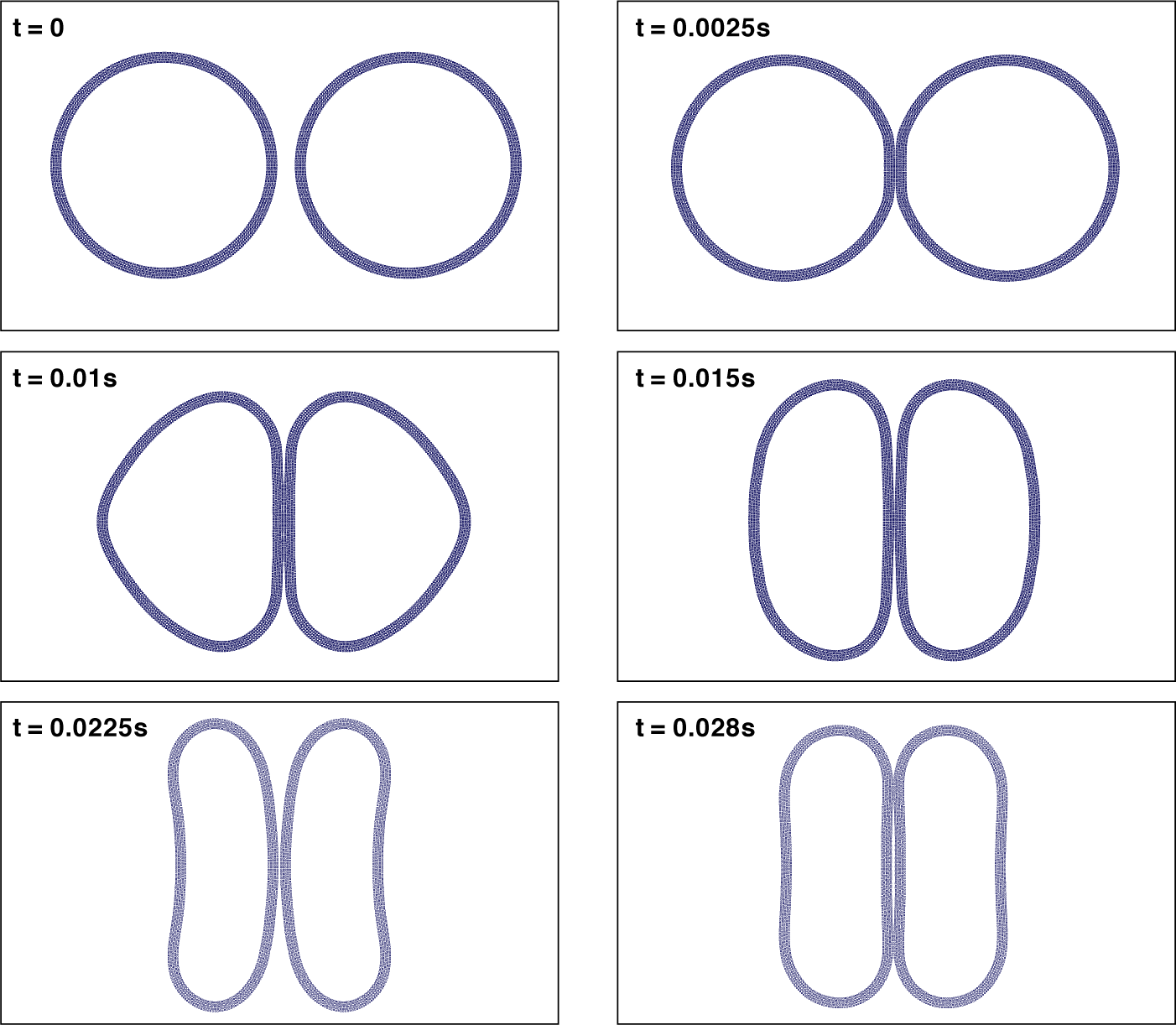
Collision of two elastic rings, each of which has a similar diameter of $0.2$
m, thickness of
$0.2$
m, thickness of $1$
cm, Young’s modulus of
$1$
cm, Young’s modulus of $20$
GPa and moves at a constant velocity
$20$
GPa and moves at a constant velocity $v_r=5$
m/s, is simulated using the ICB-SPH algorithm.
$v_r=5$
m/s, is simulated using the ICB-SPH algorithm.
To test the stability of the ICB-SPH, the rings are assumed to move at an extremely high velocity $V_r=8$
m/s. There are no cracks or odd particle configurations observed in the rings. The shape of the two rings is also seen as perfectly symmetric. As seen in Figure 10, high-frequency wave-like motions are also observed along the interface of the two rings. Such a motion is expected in strong elastic interactions where different modes and frequencies of elastic motions propagate along the rings simultaneously. As seen in Figure 10, although the two rings are significantly deformed at
$V_r=8$
m/s. There are no cracks or odd particle configurations observed in the rings. The shape of the two rings is also seen as perfectly symmetric. As seen in Figure 10, high-frequency wave-like motions are also observed along the interface of the two rings. Such a motion is expected in strong elastic interactions where different modes and frequencies of elastic motions propagate along the rings simultaneously. As seen in Figure 10, although the two rings are significantly deformed at $t=0.02$
s, the uniformity of the particle configuration is well maintained throughout the simulation. Therefore, it can be said that the ICB-SPH scheme is an ideal tool to tackle complex elastic motions with large magnitudes and high frequencies.
$t=0.02$
s, the uniformity of the particle configuration is well maintained throughout the simulation. Therefore, it can be said that the ICB-SPH scheme is an ideal tool to tackle complex elastic motions with large magnitudes and high frequencies.
Collision of two elastic rings, each of which has a similar diameter of $0.2$
m, thickness of
$0.2$
m, thickness of $1$
cm, Young’s modulus of
$1$
cm, Young’s modulus of $20$
GPa and moves at a constant velocity
$20$
GPa and moves at a constant velocity $v_r=$
8 m/s, is simulated using the ICB-SPH algorithm.
$v_r=$
8 m/s, is simulated using the ICB-SPH algorithm.
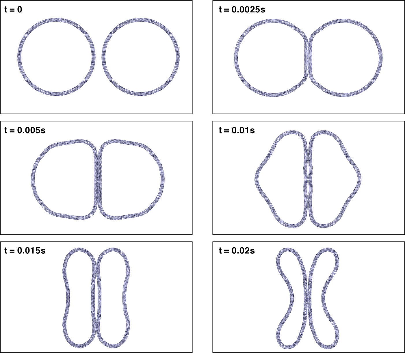
4 Conclusions
In this paper, SPH algorithms for elasticity, namely the initial configuration-based algorithm and the current configuration-based algorithm, are adopted to simulate bending of an elastic beam, extension/compression of a truss and collision of two elastic rings. The scope of the study is focusing on large elastic deformation by which the particle configuration representing the elastic structures is highly compressed and/or stretched and could lead to severe numerical errors and then instabilities for the structures. In addition, a contact force model and an equation of state are analytically developed to model the elastic collision between two rings.
For the beam-bending problem, six scenarios in which the magnitude of the vertical force is varied from $10$
N to
$10$
N to $250$
N are simulated. The simulations show that the CCB-SPH algorithm fails to maintain the structure when the force magnitude exceeds
$250$
N are simulated. The simulations show that the CCB-SPH algorithm fails to maintain the structure when the force magnitude exceeds $25$
N; with the presence of the artificial stress term, the CCBWAT-SPH algorithm can maintain the structure’s stability in all the investigated cases although numerical errors, in comparison with the corresponding theoretical values, get increasingly worse as the load is increased; and the ICB-SPH algorithm can maintain very well the uniformity of the particle configuration, as well as result in the displacement values in a very good agreement with the theoretical ones.
$25$
N; with the presence of the artificial stress term, the CCBWAT-SPH algorithm can maintain the structure’s stability in all the investigated cases although numerical errors, in comparison with the corresponding theoretical values, get increasingly worse as the load is increased; and the ICB-SPH algorithm can maintain very well the uniformity of the particle configuration, as well as result in the displacement values in a very good agreement with the theoretical ones.
For the truss extension, the CCB-SPH algorithm fails to maintain the structure in all the investigated scenarios, the CCBWAT-SPH can withstand for the load up to $3000$
N and the ICB-SPH performs well in all the cases. For the truss compression, all the algorithm can handle well the deformations, because the compressed particle configurations do not produce remarkable numerical errors for the particle approximation in SPH unless the particle distance gets smaller than
$3000$
N and the ICB-SPH performs well in all the cases. For the truss compression, all the algorithm can handle well the deformations, because the compressed particle configurations do not produce remarkable numerical errors for the particle approximation in SPH unless the particle distance gets smaller than $0.5$
of the initial particle distance at which the derivative of the weight function with respect to the particle distance is incorrectly evaluated.
$0.5$
of the initial particle distance at which the derivative of the weight function with respect to the particle distance is incorrectly evaluated.
In the simulations for the two-rings collision, large deformations and high frequency elastic oscillations cause instabilities (cracks) in the particle configuration when the CCB-SPH algorithm is used. The artificial stress term in the CCBWAT-SPH algorithm helps to reduce the effect; however, it alters the rigidity of the rings and therefore the rings are seen to be less elastic. The ICB-SPH algorithm can maintain the particle structure of the rings very well in the two tests, in which the relative velocity of the two rings is $10$
m/s and
$10$
m/s and $16$
m/s. In particular, wave-like elastic motions were also captured successfully by the ICB-SPH algorithm.
$16$
m/s. In particular, wave-like elastic motions were also captured successfully by the ICB-SPH algorithm.


 Open access