


1. INTRODUCTION
Atmospheric warming in the Antarctic Peninsula was among the strongest in the world during the latter half of the 20th century. Air temperatures rose here by over half a degree per decade between 1955 and 2005 (Turner and others, Reference Turner2005) and both surface and deep ocean temperatures in the adjacent seas increased contemporaneously (e.g. Meredith and King, Reference Meredith and King2005, Robertson and others, Reference Robertson, Visbeck, Gordon and Fahrbach2002). Atmospherically forced changes to melt intensity during this period have been strongly implicated in ice shelf thinning (e.g. Shepherd and others, Reference Shepherd, Wingham, Payne and Skvarca2003), changes to outlet glacier dynamics (e.g. Scambos and others, Reference Scambos, Bohlander, Shuman and Skvarca2004) and ice shelf collapse (e.g. Scambos and others, Reference Scambos, Hulbe, Fahnestock, Domack, Leventer, Burnett, Bindshadler, Convey and Kirby2003). For example, the collapse of the Larsen B ice shelf on the east side of the Antarctic Peninsula in 2002 has been connected with abnormally strong melt conditions observed on the Larsen C ice shelf to the south in the same year (van den Broeke, Reference van den Broeke2005). The collapse of the ice shelf has affected the way that part of the Antarctic Peninsula ice sheet flows into the sea by removing backstresses previously stabilising its outlet glaciers and has contributed a little to global sea-level rise directly (6.6 ± 1.5 µm a−1 between 1994 and 2008, Shepherd and others, Reference Shepherd2010). Since the loss of Larsen B, a two- to eightfold increase in the flow of these glaciers has been observed (Scambos and others, Reference Scambos, Bohlander, Shuman and Skvarca2004, Rignot and others, Reference Rignot, Casassa, Gogineni, Krabill, Rivera and Thomas2004). This has resulted in an ice loss equating to around one-third of the net loss from the Antarctic Peninsula ice sheet since 2002 (~9 Gta−1, Shepherd and others, Reference Shepherd2012, Berthier and others, Reference Berthier, Scambos and Shuman2012). Air temperatures across the Antarctic Peninsula have since experienced a period of cooling (Turner and others, Reference Turner2016, Oliva and others, Reference Oliva2017). However, since the Larsen Ice Shelf system is a climatically sensitive region, it is critical that we understand contemporary and potential future melting trends here specifically. The Larsen C ice shelf, for example, is much larger than Larsen B and could significantly affect the stability of the Antarctic Peninsula ice sheet, if it were to suffer a similar fate. Indeed, the remaining portion of the Larsen B ice shelf (SCAR Inlet), which currently buttresses three additional outlet glaciers, is now showing signs of weakness and imminent demise (Khazendar and others, Reference Khazendar, Borstad, Scheuchl, Rignot and Seroussi2015).
The climate over the Antarctic Peninsula is spatially heterogeneous. It stretches 1300 km from north to south and is characterised by a high (up to ~3000 m), narrow mountain chain, which affects the predominant westerly flow (e.g. van Wessem and others, Reference van Wessem2015). Air temperatures in the north of the region are typically higher than in the south, while temperatures on the west coast can be 5–10°C higher than those on the eastern side of the mountains at the same latitude (Cape and others, Reference Cape2015). Additionally, the eastern side of the Antarctic Peninsula is affected by atmospheric circulation over the Weddell Sea, changes to which have resulted in warming in recent years (Abram and others, Reference Abram2013). This warming is likely the result of stronger summer westerly winds, and an associated increase in the frequency of warm, dry, downslope winds coming off the peninsula mountains (föhn events, Marshall and others, Reference Marshall, Orr, van Lipzig and King2006). Indeed, patterns of surface melting over the Larsen Ice Shelf system are strongly influenced by föhn activity (Grosvenor and others, Reference Grosvenor, King, Choularton and Lachlan-Cope2014). Capturing the degree of this spatial variability is difficult because weather stations are sparse in space, satellite observations are sparse in time (and have difficulties with the rough terrain and typically cloudy conditions) and climate models are typically too coarse to adequately capture local scale meteorological processes (Barrand and others, Reference Barrand2013). Recent developments in regional climate modelling however, provide an opportunity by which simulations can now be reliably performed on a 5.5 km grid (regional atmospheric climate model, RACMO2.3/5.5), which is five times finer than previous capability has allowed (RACMO2.3/27, 27 km grid) and potentially offers improved model performance. While RACMO2.3/5.5 has been evaluated over the Antarctic Peninsula and is known to perform well (van Wessem and others, Reference van Wessem2016), fidelity at the regional scale does not necessarily translate to the local scale, particularly in terms of interannual variability (Medley and others, Reference Medley2013). Confidence in the ability of the model to reproduce local climate is key in model-based studies of specific regions such as individual ice shelves. Here, we evaluate both RACMO2.3/5.5 and RACMO2.3/27 estimates of temperature, atmospheric pressure and melting in the Larsen B embayment (pre- and post-collapse) using data from seven automatic weather stations (AWS) distributed widely around the area (Fig. 1). We then present RACMO-based estimates of melt and precipitation variability in the Larsen B area between 1980 and 2014 and contrast conditions before, during and after the collapse.
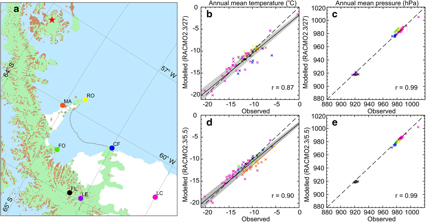
Mean annual temperature and pressure from observations and RACMO2 simulations. (a) Location of AWS stations used in evaluation, black, FL – Flask Glacier, purple, LE – Leppard Glacier, Green, FO – Foyn Point, Blue, CF – Cape Framnes, Yellow, RO – Robertson Island), pink, LC – Larsen C AWS, orange, MA – Matienzo AWS. Red star indicates location of firn core used to evaluate accumulation in RACMO2.3/5.5 in van Wessem and others (Reference van Wessem2016). Grounded ice is given in pale green, floating ice is shown in white and exposed bedrock in brown: all taken from BedMap2 (Fretwell and others, Reference Fretwell2013). Grey dotted line indicates edge of Larsen B ice shelf prior to collapse in 2002. (b–e) Modelled vs Observed mean annual temperature and pressure for all sites. Dashed lines indicate an ideal one-to-one relationship between modelled and observed values, solid lines indicate the actual fit, grey shading denotes ±1σ uncertainty on the fit. Colours represent locations as in (a) Pearson's correlation co-efficient (r) is annotated. Orange line in (d) represents a linear fit to the Matienzo data only.
2. DATA AND METHODS
2.1. RACMO2.3 regional climate model
We use the most recent version of RACMO at both low (RACMO2.3/27) and high (RACMO2.3/5.5) horizontal resolution. Details of the model can be found in van Wessem and others (Reference van Wessem2015, Reference van Wessem2016) but are summarised here. RACMO2 combines the High Resolution Limited Area Model with the European Centre for Medium-range Weather Forecasts Integrated Forecast System. RACMO2 has been adapted for use over the large ice sheets of Greenland and Antarctica: it includes a snow model (Ettema and others, Reference Ettema2010), a prognostic scheme to calculate surface albedo based on snow grain size (Kuipers Munneke and others, Reference Kuipers Munneke2011); and a routine that accounts for drifting snow (Lenaerts and others, Reference Lenaerts2012). For both model versions, ERA-Interim re-analysis data are used for forcing at the lateral boundaries. At 5.5 km, the surface topography is based on a combination of the 100 m DEM from Cook and others (Reference Cook, Murray, Luckman, Vaughan and Barrand2012) and the 1 km DEM from Bamber and others (Reference Bamber, Gomez-Dans and Griggs2009). At 27 km, the surface topography is based on Liu and others (Reference Liu, Jezek, Li and Zhao2001). At both resolutions, the ice-sheet mask includes the (former) Larsen B and Larsen A ice shelves. To investigate the potential effect of the Larsen B integration on the local near-surface climate, a separate simulation has been performed where the Larsen B ice shelf was instantaneously removed from the model ice-sheet mask, starting in the year 2003.
2.2. Observations
We assess the ability of RACMO2 to reproduce climatic variability in the Larsen ice shelf region using observations of 2 m air temperature and surface atmospheric pressure acquired by seven AWS (Fig. 1, Table S1). Larsen C AWS (WMO station number 89262) is the nearest WMO station to Larsen B with data in the years prior to collapse and is operated by the British Antarctic Survey (BAS). Observations from 1985-present are available acquired at three-hourly (i.e. one observation every 3 hours) intervals from 1985 to 2005 and 10-min intervals from 2006-present. Three-hourly temperature, but not pressure, data are also available from 1999 acquired at the Matienzo AWS, operated by the Instituto Antártico Argentino, which is located on the Seal Nunataks, at the north end of the Larsen B embayment. Since 2010, five additional AWS monitoring at up to 30 s intervals have been installed around the Larsen B embayment coincident with UNAVCO GPS monitoring sites at Flask and Leppard Glaciers, Foyn Point, Cape Framnes and Robertson Island. For comparisons with RACMO2.3/27, we pick the grid cell within which the AWS is situated. Topography is more highly variable in the high-resolution model grid relative to the low resolution, and both pressure and temperature are sensitive to height. Because of this, for comparisons with RACMO2.3/5.5 we pick the cell that has elevation most similar to that of the AWS (Table S1) within a 5 × 5 window centred on the cell in which the AWS lies, effectively ± one model grid cell in each direction. Annual values, where given, are calculated for a ‘melt year’ which is taken to be September – August inclusive (after van den Broeke, (Reference van den Broeke2005)). In order to account for fragmentation in the AWS time series (Fig. S1) and to use the maximum amount of data in our comparison, we sub-sampled the RACMO2 time series to only those periods where AWS data were available. As such, annual values for incomplete years should not be considered true values.
2.3. Positive degree-day (PDD) sum
RACMO2 estimates of melting are based on the balance of energy fluxes at the snow/ice surface. Because we do not have these data for the AWS, we use PDD as a proxy for melting calculated from both modelled and observed temperatures. PDDs and melting are typically well correlated (e.g. Braithwaite and others, Reference Braithwaite1995). For example, we find a correlation of r = 0.72 between RACMO2 estimates of total annual PDDs and melt amount averaged over the now-missing portion of the Larsen-B ice shelf. We use a PDD sum that accounts for both the duration and intensity of above zero temperature conditions (Eqn (1), Vaughan, Reference Vaughan2006).
 $$\varphi _{\rm n} = \mathop \sum \limits_{i = 1{\rm st\; September,\; year}\; n - 1}^{i = 31{\rm st\; August,\; year}\; n} T_i^{} \left( {t_{i + 1} - t_i} \right)\alpha \left( {T_i} \right),$$
where φ is annual total PDDs, T is observed/modelled 2 m temperature in °C, t is the time expressed in fractions of days and α(T i) is 1 if T is positive and 0 if T is negative. Prior to calculating PDDs we interpolate/aggregate (as appropriate) all seven sets of observations and both model versions onto a commonly sampled hourly time series (we do not gap-fill missing data), thus T in Eqn (1) is hourly temperature.
2.4. Estimating radiation errors
Unaspirated temperature sensors are prone to radiation errors under high-insolation, low wind speed conditions, which result in a temperature excess to the actual air temperature (Erell and others, Reference Erell, Leal and Maldonado2005, Huwald and others, Reference Huwald2009). Smeets (Reference Smeets2006) showed that for a Vaisala HMP45C platinum resistance thermometer this excess temperature can be estimated as a function of total shortwave radiation at-sensor and wind speed (Eqns (2) and (3)).
 $$\eqalign{\Delta T &= \; \displaystyle{k \over {(9.6\; \times \; {10}^{ - 3}k + 6.3){(12U)}^{1.25}}}\; \;{\rm for}\;\; \cr & \quad U \ge 2\,{\rm ms}^{ - 1}}.$$
 $$\Delta T = 4.14 \times 10^{ - 3}k - 0.15\; \;{\rm for}\;\; U \lt 2\,{\rm m}{\rm s}^{ - 1},$$
where ΔT is the excess temperature, U is wind speed and k is the total shortwave radiation at sensor. In the absence of observed radiation, we estimate k to be:
 $$(1 + \alpha )\tau SW_{{\rm TOA}},$$
where SW TOA is the top of the atmosphere incoming shortwave radiation, τ is the atmospheric transmissivity (0.79 for clear sky conditions in Antarctica, van den Broeke and others, Reference van den Broeke, Reijmer and van de Wal2004) and α is the surface albedo. We estimate the impact of this effect on our AWS derived PDD totals at Larsen C AWS (Fig. 2) which uses an instrument and radiation shield comparable with that described in Smeets (Reference Smeets2006). We take α to be 0.75 since this AWS is situated on snow; this can be considered a conservative estimate (Kuipers Munneke and others, Reference Kuipers Munneke, van den Broeke, King, Gray and Reijmer2012). We are unable to estimate radiation errors at Matienzo and the UNAVCO stations using this method; while Matienzo also uses a HMP45C temperature sensor it has a much larger old-style radiation shield and the UNAVCO AWS use a different type of thermometer entirely.
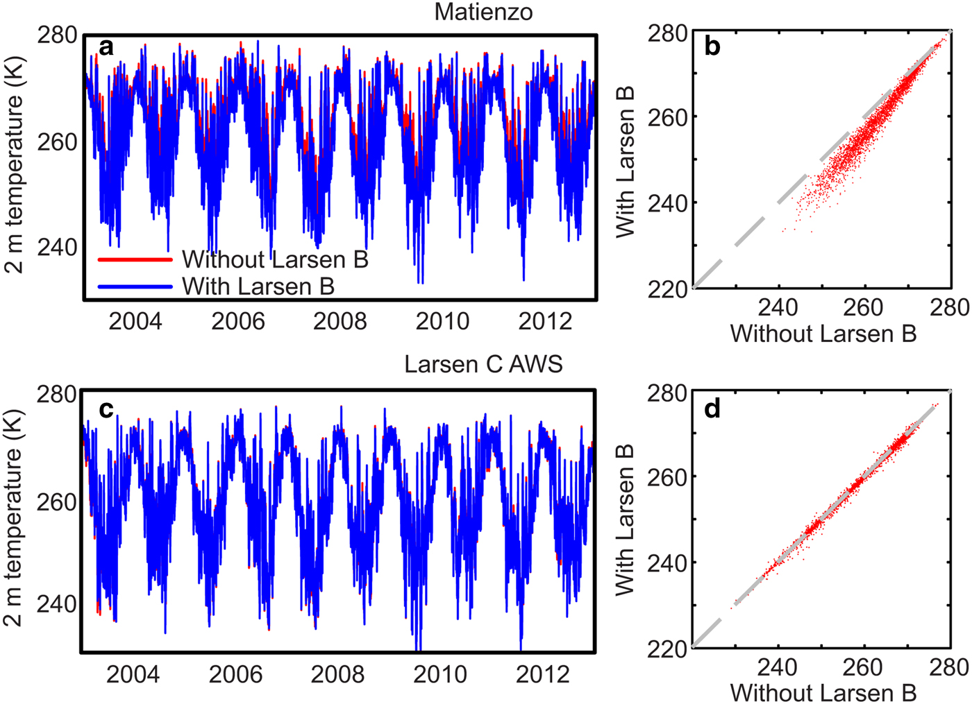
RACMO2.3/5.5 simulated temperatures for Matienzo and Larsen C AWS. (a, c) daily mean 2 m temperature with (blue) and without (red) the Larsen B ice shelf. (b, d) daily mean 2 m simulation with Larsen B vs simulation without Larsen B.
3. RESULTS AND DISCUSSION
We compare RACMO2.3/5.5 and RACMO2.3/27 simulated values for annual mean 2 m temperature and surface atmospheric pressure with observations made at the AWS (Fig. 1). Both versions of the model reproduce spatial and interannual variability in annual mean surface pressure almost exactly (r = 0.99 in both cases), which suggests that the model captures synoptic scale atmospheric conditions across the region well. Generally, both versions of the model capture interannual variability in mean annual temperature (r = 0.90 and 0.87, respectively). A slight deviation from the one-to-one line is apparent in the slope of the linear fit to these data in both model versions and suggests that RACMO is less well able to capture temperatures that are either particularly high or particularly low. Specifically, RACMO overestimates mean annual temperature in particularly cold years, and underestimates mean annual temperature in particularly warm years; this is also the case at the sub-annual timescale (Fig. S2) and in the mean, summertime only, temperatures (Fig. S3). This is potentially due to differences in the surface type; RACMO assumes that all surfaces are ice/snow covered when in fact four of the seven AWS are on bare rock, including Matienzo and Robertson Island. Due to its low albedo, relative to ice/snow, exposed rock is likely to heat up considerably in summer, potentially allowing for higher 2 m air temperatures than over snow surfaces. A paucity of observations precludes a robust assessment of precipitation, but previous evaluations show that RACMO2.3/5.5 can reproduce interannual variability in accumulation at James Ross Island (the nearest available accumulation record to Larsen B) during our study period (r = 0.75 for 1998–2007, from figure in van Wessem and others, Reference van Wessem2016).
While the simulation with higher spatial resolution (RACMO2.3/5.5) offers a slight improvement in model-observation agreement overall, the change in resolution introduces a low bias in mean annual temperature at Matienzo (~−1.8°C) and Robertson Island (~−1.6°C), which are both located on the Seal Nunataks at the interface between the Larsen B and Larsen A embayments. This is somewhat consistent with a previous study, which has shown that RACMO2.3/5.5 simulates temperatures which are too low on average (van Wessem and others Reference van Wessem2015). However, it is possible that this bias is partly due to the presence in the RACMO domain of the Larsen A (~four grid points) and B (>20 grid points) ice shelves, the former of which collapsed in 1995. We investigate the degree to which the presence/absence of Larsen B affects simulated temperatures at Larsen C and Matienzo by comparing the data with an additional RACMO2.3/5.5 simulation for the period 2003–13 in which we removed the Larsen B ice shelf from the model ice-sheet mask (Fig. 2). At Matienzo, which is closest to the Larsen B ice shelf, there is a bias of ~3°C between the two simulations; the removal of the ice shelf results in higher simulated temperatures here, presumably due to heat exchange from the (relatively) warm ocean. This is particularly evident during the winter; the bias diminishes by an order of magnitude as temperatures increase. In fact, we calculate a bias of just 0.3°C if we only include above-zero temperatures in the calculation. This can be attributed to the fact that ocean-atmosphere temperature gradients are much greater during the winter. The interannual variability in mean annual temperature is consistent between the simulations with and without the ice shelf (r = 0.99, n = 9) and the effect is very localized; we see no difference in simulated temperatures with/without the ice shelf at Larsen C.
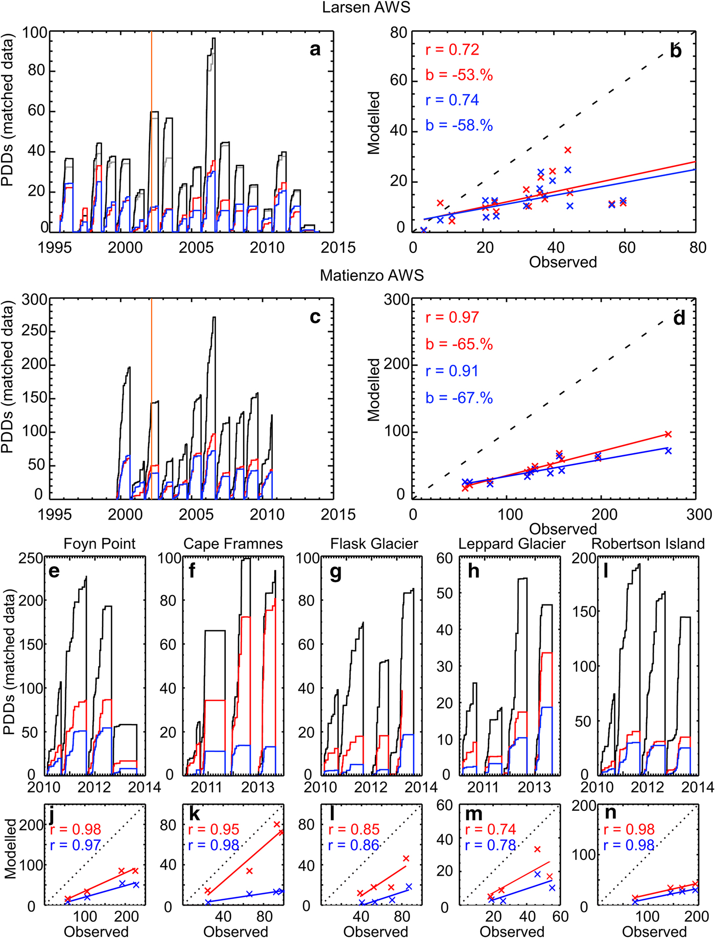
Interannual variability in total PDDs (Fig. 3) is particularly well captured by RACMO at Matienzo (r = 0.97, r = 0.91 for RACMO2.3/5.5 and RACMO2.3/27 respectively) and at Robertson Island (r = 0.98, r = 0.98), Foyn Point (r = 0.98, 0.97) and Cape Framnes (r = 0.95, r = 0.98), but less so at Larsen C AWS (r = 0.72, r = 0.74). In particular, both versions of RACMO2 ‘miss’ the particularly high PDD year in 2001/02 observed at the Larsen C AWS. The high melting observed on Larsen C in this year has been attributed to anomalous atmospheric circulation conditions (van den Broeke, Reference van den Broeke2005); predominant northeasterly winds and prolonged transport of air over open water towards the Larsen ice shelf. Presumably, this was not fully captured by the model. Both versions of RACMO2 underestimate total annual PDDs by more than half at all sites considered here except for Cape Framnes (Fig. 3). We investigate the degree to which this can be attributed to radiation errors under low wind, high insolation conditions at the AWS sensors. We subtract the calculated excess temperature (order of 1°C, see Section 2) from the observations when (1) it is daylight, (2) wind speed is <4 ms−1 and (3) wind direction is from the North West (so likely to be cloud-free, Kuipers Munneke and others, Reference Kuipers Munneke, van den Broeke, King, Gray and Reijmer2012). We find that this reduces the number of total annual PDDs by up to 30% at Larsen C (8% on average), that the effect is particularly notable in high melt years and that comparing with the corrected time series improved model performance (r = 0.82, r = 0.79). RACMO2.3/5.5 again offers an improvement against RACMO2.3/27 in predicting both PDD amount and interannual variability at Matienzo, however we note that in this case, increasing the horizontal resolution does not have a major impact on model-observation agreement. When we correct for the model bias at Matienzo (by adding 1.82°C to all modelled data) we see excellent agreement with the observations (Fig. S4). PDDs in very high melt years are underestimated slightly even with this correction; this is likely due to radiation errors at sensor. Note that while annual PDD totals do not always reflect true annual values due to sampling of observation data (e.g. Fig. S1), with the exception of 84 days between March and May in 2004, the Matienzo AWS record is complete during the period reported.
Annual PDDs modelled and observed at each AWS. Note: model has been sampled to available observations (Fig. S1). Observed values are given in black, observed (corrected) values are given in grey. Simulated values are given in blue (RACMO2.3/27) and red (RACMO2.3/5.5). Panels (a, c, e–i) show cumulative PDDs from the 1st September each year. Panels (b, d, j–n) show modelled vs observed total annual PDDs, Pearson's correlation co-efficient (r) and mean bias (b) between the observed and modelled annual values are annotated. Vertical orange line in (a) and (c) indicates timing of ice shelf collapse.
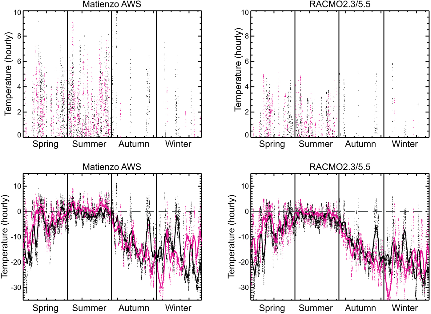
The timing of the Larsen B ice shelf collapse has been attributed to the draining of melt ponds on the ice shelf surface (Scambos and others, Reference Scambos, Hulbe, Fahnestock, Domack, Leventer, Burnett, Bindshadler, Convey and Kirby2003) coinciding with anomalously strong melt conditions observed at the Larsen C AWS (van den Broeke, Reference van den Broeke2005). However, the AWS data presented here show that while the number of PDDs at Matienzo in the year of collapse was above average (145 in 2001/02, 7% greater than the 1999–2010 mean value), the total PDD amount 2 years prior to collapse (1999/2000) was 30% higher. Previous work based on these data has reported that, of the 2 years, 2001/02 had more days where the temperature rose above zero (Skvarca and others, Reference Skvarca, De Angelis and Zakrajsek2004). Our analysis agrees with this (Table 1), but we find that there were significantly more hours with above zero temperatures in 1999/2000 than in 2001/02 and that the average above-zero temperature was almost half a degree higher. This results in more PDDs in 1999/2000 than 2001/02, when calculated using our method, which takes both duration and magnitude of above-zero temperature events into account. It has also been noted previously that 2001/02 had a warmer summer in the Larsen B region than 1999/2000 (Cape and others, Reference Cape2015). We also see this in our analysis (Fig. 4) but note that the autumn of 1999/2000 was particularly warm. This accounts for the fact that we calculate a continued accumulation of PDDs after the end of the summer in 1999/2000 but not in 2001/02. These signals appear in both the Matienzo AWS data and the RACMO simulation, which can be considered independent.
Temperature during 1999/2000 (black) and 2001/02 (pink) observed at the Matienzo AWS and simulated by the RACMO2.3/5.5 model. Bottom: full temperature range, top: above zero temperatures only. Solid lines show data smoothed with a 7-day window.
Summary of the above zero conditions as observed at the Matienzo AWS and simulated by RACMO2.3/5.5 in 1999/2000 and 2001/02
Of the 2 years, although 1999/2000 had more PDDs than 2001/02 at Matienzo, we agree with previous findings that the latter was, in fact, the higher melt year of the two at Larsen C AWS (60 PDDs in 2001/202, 100% greater than the 1996–2012 average with 2004–06 and 2012 excluded due to missing data, Fig. S1). The Larsen C AWS is ~220 km further south than the now-missing portion of the Larsen B ice shelf. However, it is unlikely that this distance is large enough to explain differences in the PDD signal between the two sites. The anomalous atmospheric circulation conditions promoting high melting on Larsen C (van den Broeke, Reference van den Broeke2005) would likely have also affected Larsen B. We attribute this high degree of spatial variability to differences in the relationship between melting and föhn wind events. Larsen C AWS is further away from the Antarctic Peninsula Mountains than Matienzo and so is unlikely to be as strongly affected by föhn warming. Total melt in the northern part of the Larsen B embayment (particularly over the Seal Nunataks) is more highly correlated with föhn activity than on Larsen C (r > 0.5 and r < 0.5, respectively during 1999–2010, Cape and others, Reference Cape2015). In fact, total annual PDDs and number of föhn days observed at Matienzo (ibid) are highly correlated (r = 0.72). Our finding that the RACMO2.3/5.5 model reproduces temporal variability in total annual PDDs at Matienzo with a high degree of fidelity (especially when temperatures are bias corrected) suggests that RACMO2.3/5.5 is able to represent local scale processes controlling melt such as the frequency of föhn winds. However, further work is needed to confirm that this is generally the case, and not just confined to this location.
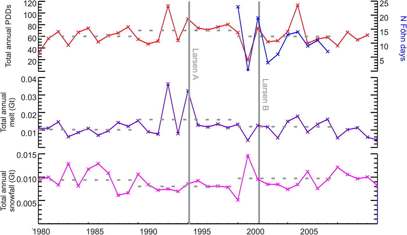
In the longer term context (1980–2014, Fig. 5, Table 2); we see from RACMO2.3/5.5 that the 1990s were a climatologically anomalous decade. Although mean annual temperature generally declined between 1980 and 2014, summer (DJF) temperatures in the 1990s (−2.35°C on average, σ = 0.88) were higher than in the 1980s (−2.68°C, σ = 0.51) and in the 2000s (−2.61°C, σ = 0.77). Similarly, melting was stronger and precipitation lower in the 1990s than in either the decade before or after. We use multivariate changepoint analysis (Killick and others, Reference Killick, Fearnhead and Eckley2012, see supplementary methods) to assess the degree to which this difference is statistically sound and detect changepoints at 1992, 1996 and 1999, in general showing that melting and snowfall in the 1990s was statistically different to that before and since (Fig. S5). This is consistent with the findings of Turner and others (Reference Turner2016) who show that air temperature increased and then decreased during this period with the transition from ‘warming’ to ‘cooling’ occurring ~1998–99. Turner and others (Reference Turner2016) attribute the pre-1999 warming to a positive trend in the Southern Annular Mode increasing the flow of mild, northwesterly air, which is likely to have been amplified through the föhn effect in the Larsen B region. Melting can contribute to ice shelf break-up if supraglacial lakes are able to form and drain, however a condition of supraglacial lake formation is the depletion of firn pore space (KuipersMunneke and others, Reference Kuipers Munneke, Ligtenberg, van den Broeke and Vaughan2014), which is achieved when snowfall is low and/or melting is high. A high degree of melting in the decade before the collapse of the Larsen B ice shelf in 2002 is therefore consistent with previous findings that multiple strong melt years are required to deplete firn pore space and weaken an ice shelf before it can fail (Trusel and others, Reference Trusel2015). The apparent ‘return’ to 1980s levels of melting after break up is also consistent with the wider pattern of decadal-scale atmospheric cooling observed in the region since then (Turner and others, Reference Turner2016, Oliva and others, Reference Oliva2017) and may have provided for a period of stability for the remnants of Larsen B, including Scar Inlet. The RACMO2 simulation also shows that the year before collapse – 2000/01 – was characterised by the lowest amount of melting (0.004 Gt, one third of the average value) and the highest amount of snowfall (0.0145 Gt, 60% higher than average) of the 35 year period. Further investigation is required to determine whether these conditions played a role in the collapse event, but potential avenues for enquiry include the impact of higher than usual snow loading on the weakened ice shelf, and the impact of refreezing/latent heat release within the thicker than usual snowpack.
RACMO2.3/5.5 estimates of annual PDDs (based on 3-hourly 2 m air temperature, red), melting (purple) and snowfall (pink), averaged over the now-missing portion of the Larsen B ice shelf. Number of föhn days at Matienzo (blue, Cape and others, Reference Cape2015). Solid gray vertical lines refer to the Larsen A and Larsen B ice shelf collapse events. Dashed grey horizontal lines represent decadal mean values.
Decadal average 2 m temperature, PDDs, melt and precipitation over the now-missing portion of the Larsen B ice shelf, as simulated by RACMO2.3/5.5
4. CONCLUSIONS
We use observations of temperature and pressure taken at seven AWS evenly distributed around the Larsen B embayment to show that both RACMO2.3/27 and RACMO2.3/5.5 simulate interannual variability in mean annual temperature and pressure well. However, we identify a systematic low bias in simulated temperatures in the northernmost part of the region. We attribute this to a range of factors including a general low bias in the model, the presence of the Larsen A and B ice shelves in the simulation post-collapse, excess warming at-sensor under low wind, high insolation conditions and differences between the real (bare rock) and modelled (ice) surface conditions. We show that, in this location, both versions of RACMO2 over-estimate particularly low temperatures and under-estimate particularly high temperatures. Because of this, RACMO2 based estimates of total annual PDDs are lower than observed values, although the model captures interannual variability well. This suggests that RACMO2 can reliably be used to investigate interannual variability in melting (known to be correlated with PDDs) in this region. We note that RACMO2-based estimates of melting are calculated using a full surface energy balance and that these estimates have been shown to perform reasonably well in Antarctica in general (Trusel and others, Reference Trusel, Frey, Das, Kuipers Munneke and van den Broeke2013), although a detailed assessment at this specific location has yet to be completed. Nonetheless, we show that when corrected for the observed systematic temperature bias, RACMO2.3/5.5 reproduces PDD amount in the northern part of the region almost exactly. Using RACMO2.3/5.5, in conjunction with AWS data, to investigate longer-term patterns in melting and precipitation in this sector, we see that while the year of the Larsen B ice shelf collapse (2002) was a high melt year, melting was not as high as in the 1999/2000 melt season, 2 years previously. In addition, we see that the year prior to break-up exhibited the lowest melting and highest precipitation on record. The decade prior to collapse was characterised by a series of strong melt and low precipitation years, which likely pre-conditioned the ice shelf to collapse. However, since then, melting and precipitation have returned to pre 1990's values, which potentially explains why we have yet to see further, substantial, ice shelf collapse in this region.
5. ACCESS TO DATA AND ACKNOWLEDGEMENTS
Larsen C AWS data are available via request from Steve Colwell (src@bas.ac.uk), Matienzo AWS data are available from Pedro Skvarca (pedroskvarca@gmail.com) and Sebastian Marinsek (smarinsek@dna.gov.ar) and UNAVCO AWS data can be accessed here: https://www.unavco.org/data/tropospheric/surface-met/surface-met.html. RACMO2 model output is available on request from J. M. van Wessem. The R package used to perform multivariate changepoint analysis (changepoint.mv) is soon to be released on (the comprehensive R network) CRAN, and is available from Rebecca Killick (r.killick@lancaster.ac.uk). MRvdB, SRML and JMvW acknowledge funding from the Polar Program of the Netherlands Organization for Scientific Research (NWO/NPP) and the Netherlands Earth System Science Centre (NESSC).
SUPPLEMENTARY MATERIAL
The supplementary material for this article can be found at https://doi.org/10.1017/jog.2017.39.


 Open access