


1. Introduction
In a seminal paper, Arnott and Small Reference Arnott and Small(1994) noted that traffic congestion in metropolitan areas has become a major plague of modern society. Thirty-one years later, the populations of large cities around the world have grown significantly, the number of cars on the road has proliferated, delay times have increased markedly, and despite billions of dollars, yen, and euros spent expanding the capacity of road networks and constructing new roads, the negative effects of congestion have worsened. There seems to be no quick fix for traffic congestion. The magnitude of the congestion problem in large metropolitan areas is so enormous that no single policy can address it. Rather, the problem requires multiple strategies, where each strategy represents a component of a broader solution.
The most obvious strategies include expanding the capacity of existing roads; constructing new roads, railways, and bridges; assigning priority by designating special lanes for public transport and carpooling; and imposing driving restrictions on selected days. Although these strategies may seem intuitive, under certain conditions, some can yield counterintuitive results. Several paradoxical outcomes have been discussed in the literature on transportation science, operations research, and computer science. These studies show that, under specific conditions related to network architecture, the number of users, and the costs of alternative modes of transportation, attempts to reduce congestion by expanding traffic networks may prove ineffective. Specifically, the Pigou-Knight-Downs (P-K-D) paradox (Pigou, Reference Pigou1920, Knight, Reference Knight1924, Downs, Reference Downs1962) states that, under certain conditions, expanding road capacity may not achieve the goal of reducing travel cost. The Braess Paradox (Braess, Reference Braess1968) indicates that expanding a traffic network by adding one or more routes may paradoxically increase the equilibrium cost of commuting. The Downs-Thomson (D-T) paradox (Downs, Reference Downs1962, Thomson, Reference Thomson1978), which is the focus of our study, posits that under certain conditions, increasing road capacity when commuters face a choice between private and public transportation modes may prove ineffective as it may not decrease the overall cost of travel.
The three paradoxes above have been presented, discussed, and illustrated numerically in the theoretical literature (see, for example, Arnott and Small, Reference Arnott and Small1994, Rapoport and Mak, Reference Rapoport, Mak, Donohue, Katok and Leider2018). Empirical evidence dates back to Mogridge Reference Mogridge(1990), who reported that increased road capacity in central London coincided with a decline in mass transit systems, supporting the D-T paradox. Indirect evidence supporting the Braess paradox has been reported, among others, by Murchland Reference Murchland(1970) and Youn et al. Reference Youn, Gastner and Jeong(2008).
Horowitz Reference Horowitz(1984) noted that field data on route choices or choices between private and public transportation cannot resolve whether equilibrium solutions accurately describe behavior in real traffic networks. In their study of the D-T paradox, Dechenaux et al. Reference Dechenaux, Mago and Razzolini(2014) argue that “The variety and complexity of ways in which current travel decisions may depend on past network performance, and the complete lack of empirical information about the form of this dependence, renders the usefulness of ‘natural experiments’ in real networks doubtful” (p.463). An alternative way to test the validity of the equilibrium solutions of these paradoxes is through controlled laboratory experiments, in which participants are incentivized by monetary payoffs contingent on their performance. These experiments present a powerful technique for answering theoretical questions regarding the descriptive power of equilibrium solutions. One of their advantages is their ability to manipulate key variables in traffic networks (e.g., transportation cost, group size, scheduling of traffic, and information structure) that influence commuters’ choices and may give rise to the paradoxes described above.
In the theoretical and experimental studies of the D-T paradox, the population typically consists of homogeneous agents: all commuters face the same cost structure and make independent choices between public and private transportation. Departing from this standard setting, we propose a novel scenario that combines elements of the D-T paradox with elements of queuing theory. As in the D-T paradox, our model features two distinct transportation modes, private car and railway, that connect a common origin (e.g., residential area) and a common destination (e.g., central business area). Unlike the standard D-T setting, the road in our scenario is known to have a single bottleneck with a fixed capacity that compels drivers to trade off the cost of queuing delay at the bottleneck with the cost of schedule delay (i.e., the cost of arriving early or late). In our model, each commuter is asked independently to make two decisions: which mode of transportation to use, and if choosing to travel by car, at what time to depart from the origin. An important implication of this scenario is that improving the road (e.g., by reducing service time at the bottleneck) may affect not only the number of commuters choosing to travel by car but also the distribution of their departure times. In equilibrium, although arrival times may differ, travel costs must be equal across commuters.
Another departure from the standard D-T scenario is our assumption that the railway operator’s response to changes in passenger volume is perfectly inelastic. Improving the road may attract train commuters from the railway, thereby reducing revenue for the railway operator. If revenue falls while costs remain fixed or rise, the operator may need to increase fares or reduce service frequency, further pushing commuters toward the road. Therefore, road improvement may completely dissipate its benefits and even worsen overall travel cost. However, we assume that the railway operator does not modify its service quality from day to day to avoid disruptions to commuters. Consequently, the travel cost of train commuters is independent of passenger volume and depends solely on train travel time. If the railway operator shortens train travel time, some car commuters may switch from the road to the railway. Therefore, the D-T hypothesis we set to test is that improving the railway may decrease mean travel cost, but improving the road may keep mean travel cost unchanged.
The goal of this study is to experimentally investigate a novel scenario that embeds the D-T paradox in the context of departure-time choice in the morning commute (for example, Vickrey, Reference Vickrey1969, Arnott et al., Reference Arnott, de Palma and Lindsey1990, Arnott et al., Reference Arnott, de Palma and Lindsey1993). Commuters opting to travel by car must also choose when to depart from the origin to trade off the costs of queuing delay due to congestion at the bottleneck and the schedule delay costs associated with their time of arrival at their common destination. We numerically derive a symmetric mixed-strategy equilibrium for the probability of choosing between private (congestible) and public (non-congestible) transportation, for the probability distribution of (discrete) departure times from the common origin for commuters who choose traveling by car, and for the effects of improving either the road or railway on the equilibrium cost of travel.
The remainder of this paper is organized as follows. Section 2 presents a brief literature review of theoretical and experimental studies related to the present study. Section 3 introduces the notation, formally describes the model, illustrates it with a numerical example, and presents the symmetric mixed-strategy equilibrium solution. Section 4 outlines the experimental design and methods. Section 5 presents and discusses the experimental results. Section 6 proposes a reinforcement learning model. Section 7 concludes the study with a summary of the results.
2. Literature review
The D-T paradox was introduced by Downs Reference Downs(1962) and subsequently studied, among others, by Thomson Reference Thomson(1978), Mogridge Reference Mogridge(1990), Mogridge et al. Reference Mogridge, Holden, Bird and Terzis(1987), Calvert Reference Calvert(1997), and Afimeimounga et al. Reference Afimeimounga, Solomon and Ziedins(2005). Ding and Song Reference Ding and Song(2012) have presented a technical introduction that allows a comparison between the P-K-D, Braess, and D-T paradoxes. The D-T paradox concerns a directed network with two parallel routes (or modes of transportation) that connect a common origin with a common destination. Travel on the private route generates negative externalities, whereas travel on the public route generates either positive externalities or no externalities. Under certain conditions on the cost structure and size of the user population (see, for example, Ding & Song, Reference Ding and Song2012), the expansion of the road produces no change in or even a decline in social welfare due to a shift in the equilibrium. Network users shift from the public to the private mode of transportation, thereby generating additional negative externalities, which, in turn, may reduce social welfare.
Denant-Boèmont and Hammiche Reference Denant-Boèmont and Hammiche(2010) conducted a study of the D-T paradox that included a two-stage coordination game. In Stage 1, a single participant (called “operator”) chose the capacity of the public route, whereas the cost of the private route was chosen exogenously by the experimenter. In stage 2, multiple group members were asked to choose between the private and public modes of transportation. The road capacity was systematically manipulated across iterations. The authors reported three major findings. First, the D-T paradox was realized. Second, the mean route choices approached the equilibrium solution across iterations of the stage game. Third, there was no support for equilibrium play by the operator in Stage 1 of the D-T game. Dechenaux et al. Reference Dechenaux, Mago and Razzolini(2014) conducted a second, single-stage, game in which the cost of the public route was determined exogenously and remained fixed over iterations of the stage game whereas the cost of the private route was changed systematically. Travel costs and group sizes were manipulated in the experiment. The authors report evidence in support of the D-T paradox as well as the systematic effects of group size and travel costs on public route choices.
Our study differs markedly from these two previous studies in its setup. The players in our study make two simultaneous decisions: which mode of transportation to choose (congestible versus. non-congestible), and, for those choosing the congestible mode, when to depart from their common origin. Unlike the previous two studies, we do not merely focus on the number of group members who choose to travel by car or train. Rather, we test both the choice of transport and changes in the distributions of departure time. The cost structure of the model (presented in Section 3) reflects these two decisions. In addition, whereas the travel cost on the public route (“metro”) in the experiment reported by Dechenaux et al. Reference Dechenaux, Mago and Razzolini(2014) was set to decrease in the number of users, it was fixed exogenously in our study.
Another major difference from the two previous studies is in what happens on the congestible road and the method used to derive the symmetric mixed-strategy equilibrium. Whereas the cost of traversing the road is commonly determined by a simple function of the number of users, we employ the first-come, first-served (FCFS) queue discipline at the bottleneck, which states that players are handled in the order of their arrival and as soon as space becomes available. This means that the cost to a car commuter departing at time t depends not only on the number of other car commuters choosing the same departure time, but also on the departure time distribution of other car commuters that left at or before time t − 1. This implies that future departures are irrelevant to the travel costs of past and current departures. As in the two previous studies, we search for the equilibrium using the key property of equalizing travel costs across departure modes and times. However, owing to the FCFS discipline, we must sequentially search for equilibrium probabilities from the earliest departure time through the last departure time.
3. Model and equilibrium
3.1. The model
Two alternative transportation modes connect a common origin and a common destination. Each of n symmetric commuters wishes to travel from the origin to the destination by either car (congestible mode) or train (non-congestible mode). All commuters wish to arrive at their destination at time  $t^{\ast}$. If a commuter chooses to travel by car, they select a departure time from a commonly known set of discrete departure times $\{1,2,\dots,t^{\ast},\dots,t_{L}\}$. If they choose to travel by train, they board a train that departs at a fixed scheduled time. Commuters independently choose both the mode and the time of departure from the origin; each of them chooses a time $t\in T=\{1,2,\dots,t^{\ast},\dots,t_{L}\}\cup\{\text{train}\}$, where “train” stands for the choice of using the public service. Commuters cannot observe the decisions of other group members when they make their own choices.
3.1.1. Travel cost: Private car commuters
First, consider the case of a commuter who chooses to travel by private car. Following Arnott et al. Reference Arnott, de Palma and Lindsey(1990), Arnott et al. Reference Arnott, de Palma and Lindsey(1993), we model congestion as a queue forming at a single section, referred to as a bottleneck (e.g., a road segment under construction, a tunnel, a single-lane bridge, or an inspection station), where the FCFS queuing discipline is applied. The bottleneck serves only one car at a time, with a service time of  $s\;( \gt 1)$ time units per car. Thus, if a driver enters the bottleneck at time t, only that driver occupies the bottleneck for s time units. As in Arnott et al. Reference Arnott, de Palma and Lindsey(1990), Arnott et al. Reference Arnott, de Palma and Lindsey(1993), this model assumes zero travel time between the origin and bottleneck entrance and between the bottleneck exit and destination. This assumption implies that a commuter traveling by car arrives at the bottleneck as soon as they depart from the origin and arrives at the destination as soon as they depart the bottleneck. If multiple commuters depart simultaneously (and consequently arriving at the bottleneck at the same time), entry order is determined randomly with equal probability.
In addition to the fixed service time s, car commuters may have to wait for an additional time at the bottleneck.Footnote 1 Suppose that car commuter i departs from the origin at time t. Then, their waiting time depends on the number of car commuters who have already departed before time t and have not exited the bottleneck, and the ones departing at time t. For each t, we denote by  $\omega_{t-1}\in \Omega$ the state of the road at the end of t − 1, which is characterized by a vector with three components $[r\;q\;e]$, where
• r: number of other commuters remaining at the origin,
• q: number of other car commuters forming a queue at the bottleneck,
• e: time elapsed since the bottleneck became occupied.
Suppose that  $\omega_{t-1}=[r\;q\;e]$, that the d other commuters (out of r) also depart by car at time t, and that k of them are ahead of commuter i after the tie is broken with equal probability. Then, commuter i’s waiting time falls into one of the eight exhaustive cases below:
 \begin{equation*}
W(t,\omega_{t-1},k)=
\begin{cases}
0&\text{if}\;r=0,q=0,e=0\\
s(q-1)+(s-1)&\text{if}\;r=0,q \gt 0,e=0\\
sq+(s-1-e)&\text{if}\;r=0,\text{any}\;q,0 \lt e \lt s\\
sq&\text{if}\;r=0,\text{any}\;q,e=s-1\\
sk&\text{if}\;r \gt 0,q=0,e=0\\
s(q-1+k)+(s-1)&\text{if}\;r \gt 0,q \gt 0,e=0\\
s(q+k)+(s-1-e)&\text{if}\;r \gt 0,\text{any}\;q,0 \lt e \lt s\\
s(q+k)&\text{if}\;r \gt 0,\text{any}\;q,e=s-1\\
\end{cases}
\end{equation*}
\begin{equation*}
W(t,\omega_{t-1},k)=
\begin{cases}
0&\text{if}\;r=0,q=0,e=0\\
s(q-1)+(s-1)&\text{if}\;r=0,q \gt 0,e=0\\
sq+(s-1-e)&\text{if}\;r=0,\text{any}\;q,0 \lt e \lt s\\
sq&\text{if}\;r=0,\text{any}\;q,e=s-1\\
sk&\text{if}\;r \gt 0,q=0,e=0\\
s(q-1+k)+(s-1)&\text{if}\;r \gt 0,q \gt 0,e=0\\
s(q+k)+(s-1-e)&\text{if}\;r \gt 0,\text{any}\;q,0 \lt e \lt s\\
s(q+k)&\text{if}\;r \gt 0,\text{any}\;q,e=s-1\\
\end{cases}
\end{equation*} Commuter i’s travel time by car is equal to the sum of their service and waiting times. Then, given  $\omega_{t-1}$ and a value of k, i’s travel time from departing at time t is
 \begin{equation*}
T(t,\omega_{t-1},k)=s+W(t,\omega_{t-1},k).
\end{equation*}
\begin{equation*}
T(t,\omega_{t-1},k)=s+W(t,\omega_{t-1},k).
\end{equation*} Car commuters experience two sources of disutility (i.e., cost). The first source results from travel time: the longer the travel time, the higher the cost to the commuters. Additionally, each commuter may incur the cost of arriving early or late, which is known as the schedule delay cost. This second source is because a car commuter must wait until work starts if they arrive at work too early, and they bear a penalty if they arrive too late. The degree of schedule delay is measured relative to the common desired arrival time  $t^{\ast}$. Therefore, for given $\omega_{t-1}$ and k, car commuter i’s total travel cost is given by
 \begin{align*}
C(t,\omega_{t-1},k)=&\;\alpha T(t,\omega_{t-1},k)\\
&+\beta \max\bigg\{0,t^{\ast}-\Big(t+T(t,\omega_{t-1},k)\Big)\bigg\}\\
&+\gamma \max\bigg\{0,\Big(t+T(t,\omega_{t-1},k)-t^{\ast}\Big)\bigg\}
\end{align*}
\begin{align*}
C(t,\omega_{t-1},k)=&\;\alpha T(t,\omega_{t-1},k)\\
&+\beta \max\bigg\{0,t^{\ast}-\Big(t+T(t,\omega_{t-1},k)\Big)\bigg\}\\
&+\gamma \max\bigg\{0,\Big(t+T(t,\omega_{t-1},k)-t^{\ast}\Big)\bigg\}
\end{align*} where the parameters α, β, and γ denote the unit costs of traveling, arriving early, and arriving late, respectively. In accordance with Small Reference Small(1982), we assume  $\gamma \gt \alpha \gt \beta$.
3.1.2. Travel cost: Public train commuter
Unlike the standard D-T scenario, the travel cost for train commuters is assumed to be fixed. There is a single commuter train that departs from the origin at time t train ( $1\leq t_{\text{train}} \lt t^{\ast}$) and arrives at the common destination precisely at the desired arrival time $t^{\ast}$, regardless of how crowded it is. The cost of traveling by train is given by
 \begin{equation*}
C_{\text{train}}=\alpha (t^{\ast}-t_{\text{train}}),
\end{equation*}
\begin{equation*}
C_{\text{train}}=\alpha (t^{\ast}-t_{\text{train}}),
\end{equation*} which reflects only the time spent in transit; it does not include train fares and assumes no economies of scale.Footnote 2 We also assume that  $t_{\text{train}} \gt s$ to ensure that there is no symmetric equilibrium in which all commuters travel by train.Footnote 3
3.2. A numerical example
Table 1 presents a numerical example that illustrates the computation of travel cost in our study. Columns 2 through 7 of Table 1 list the transportation mode, departure time from the origin, waiting time at the bottleneck, service time, arrival time at the destination, and individual travel cost, respectively. In this example, the parameter tuple is  $(n,t^{\ast},t_{\text{L}},t_{\text{train}},s,\alpha,\beta,\gamma)=(20,50,60,26,4,10,5,25)$. The table shows that departing by car does not always result in a lower travel cost, that departing too late can lead to a high cost, and that traveling by train is not always optimal.
Numerical example for  $(n,t^{\ast},t_{\text{L}},t_{\text{train}},s,\alpha, \beta,\gamma)=(20,50,60,26,4,10,5,25)$

The earliest departure occurs at t = 1, by commuter 11. Since this commuter encounters no congestion, the travel time is 4 units (i.e., zero waiting time plus 4 units of service time). Commuter 11 arrives at the destination at time t = 5, 45 time units before  $t^{\ast}=50$ (the desired arrival time). Consequently, the travel cost is 265 ( $=10\times 4+5\times 45$). Car commuters 8 and 12 depart at time t = 20. At that time, commuter 9 is being served at the bottleneck, and commuter 14 is waiting in the queue. The tie between commuters 8 and 12 is resolved randomly with equal probability, in favor of commuter 8. Commuter 8 waits 8 units at the bottleneck until the services for commuters 9 and 14 are completed. The travel time for commuter 8 is 12 units (8 units of waiting time plus 4 units of service time), leading to an arrival time of t = 32, which is 18 units before time $t^{\ast}$. The travel cost is 210 ( $=10\times 12+5\times 18$). Commuter 12, who enters the bottleneck after commuter 8, waits 12 units of time until the services for commuters 9, 14, and 8 are completed. The travel time is 16 units (12 units of waiting time plus 4 units of service time), resulting in an arrival at t = 36, 14 units before $t^{\ast}$. The travel cost in this case is 230 ( $=10\times 16 +5\times 14$).
Five commuters (2, 10, 15, 17, and 18) travel by train, departing at t = 26 and arriving at  $t^{\ast}=50$ (the desired arrival time). Since the travel time for each train commuter is 24 units, the cost for each is 240 ( $=10\times24$). The right-hand column of Table 1 shows that commuter 20, who departs at t = 16, incurs the lowest travel cost (C = 190), whereas commuter 13, who departs at t = 45 by car, incurs the highest travel cost (C = 540). The mean travel cost among the 15 car commuters is $249.7 \gt 240$.
3.3. Symmetric mixed-strategy equilibrium
This study considers the symmetric equilibrium in mixed strategies for two reasons. First, the commuters are ex-ante symmetric; the same set of strategies and cost structure hold for every commuter. Second, in asymmetric equilibria, commuters must behave differently, resulting in asymmetry in their travel costs. This implies that, without any opportunity for pre-play communication, commuters must tacitly reach an agreement on who incurs a higher travel cost and who enjoys a lower travel cost.
Figure 1 displays the equilibrium cumulative distributions of strategies, 60 discrete departure times and the train option, for the three experimental conditions: Baseline, Railway Improved, and Road Improved.Footnote 4 In the figure, the train option appears at the far right of the horizontal axis. The three experimental conditions differ in two key parameters: the service time at the bottleneck (s) and the schedule train departure time (t train):  $(s,t_{\text{train}})=(4,26)$ in the Baseline condition, $(4,30)$ in the Railway Improved condition (representing a shorter train travel time), and $(3,26)$ in the Road Improved condition (representing a reduced bottleneck service time). The corresponding equilibrium costs of travel are 240 in the Baseline and Road Improved conditions and 200 in the Railway Improved condition. The equilibrium probabilities of choosing to travel by train are 0.467 for the Baseline condition, 0.595 for the Railway Improved condition, and 0.206 for the Road Improved condition. The equilibrium support for departure times ranges from t = 7 to t = 47 in the Baseline condition, t = 15 to t = 46 in the Railway Improved condition, and t = 6 to t = 50 in the Road Improved condition.
Equilibrium cumulative probability distributions of strategies

Figure 1 illustrates two key implications of the equilibrium solution. First, shortening the travel time by train from 24 to 20 results in a shift of car commuters to the improved railway and a consequent redistribution of the departure times of car commuters until the travel costs on both modes equalize at 200. Thus, improving the congestion-free railway reduces the travel costs on both transportation modes. Second, improving the road by reducing the duration of service time at the bottleneck from 4 units to 3 units induces a shift of train commuters to the upgraded road and a redistribution of the departure times of car commuters until the travel costs for both the road and railway are equalized at 240. In other words, the benefits resulting from expanding the bottleneck are completely dissipated, in accordance with the D-T paradox. Based on the equilibrium solution, we derive the following testable hypothesis concerning the D-T paradox:
Hypothesis.
(D-T Hypothesis): Railway improvement decreases the mean travel cost, whereas road improvement does not change it.
The symmetric mixed-strategy equilibrium is inefficient in minimizing total travel cost. As a complementary benchmark, we heuristically derived the social optimum for each condition, following Arnott et al. Reference Arnott, de Palma and Lindsey(1990). First, all car commuters depart at different departure times. Second, the departure times of any two car commuters are separated by an interval equal to the bottleneck service time. These two conditions ensure that, during rush hour, no queue forms at the bottleneck and the bottleneck is never idle. Third, neither the first nor the last car commuter wants to unilaterally move to the other end of the rush hour.
Table 2 presents the number of car commuters, departure times, and the mean, minimum, and maximum travel costs in the social optimum separately for each condition. We identified seven such combinations in the Baseline condition, and two combinations each in the Rail Improved and Road Improved conditions. Two observations follow. First, although total travel cost is minimized in the social optimum, individual travel costs vary considerably across commuters. This implies that commuters incurring higher travel costs, such as car commuters assigned early or late departure times or train commuters, have a strong incentive for unilateral deviation. Indeed, these social optima do not constitute pure-strategy equilibria.Footnote 5 Second, the three conditions differ in the extent of inefficiency. The ratio of the equilibrium travel cost to the travel cost in the social optimum, known as the price of anarchy (Koutsoupias and Papadimitriou, Reference Koutsoupias, Papadimitriou, Meinel and Tison1999, Papadimitriou, Reference Papadimitriou2001, Mak and Rapoport, Reference Mak and Rapoport2013), is  $1.33\ \big(=\frac{240}{180}\big)$ in the Baseline condition, $1.24\ \big(=\frac{200}{161}\big)$ in the Railway Improved condition, and $1.58\ \big(=\frac{240}{151.5}\big)$ in the Road Improved condition. Thus, relative to the Baseline condition, railway improvement enhances efficiency, whereas road improvement worsens efficiency.Footnote 6
Number of car commuters, their departure times, and the mean, minimum, and maximum travel costs in the social optimum for  $(n,t^{\ast},t_{\text{L}},\alpha, \beta,\gamma)=(20,50,60,10,5,25)$
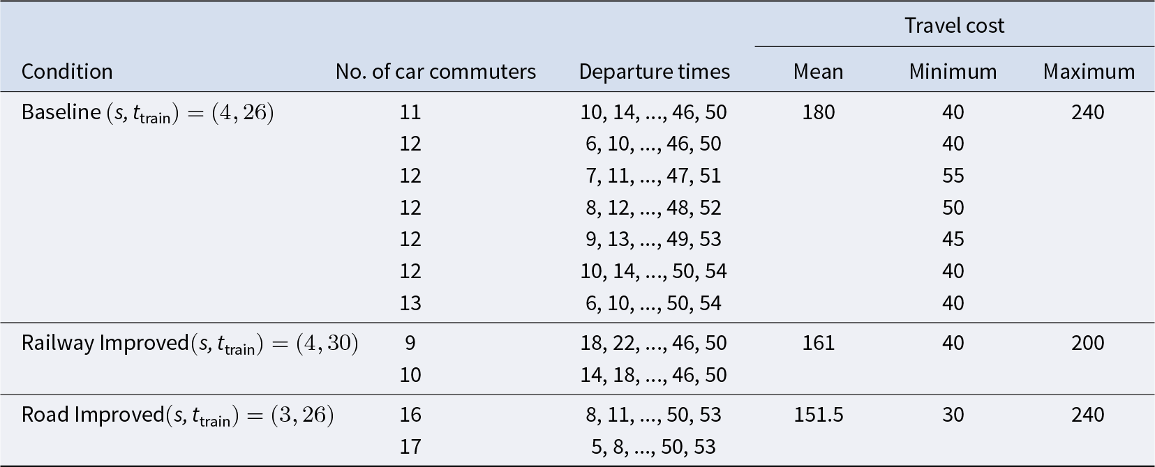
Figure 1 also displays the socially optimal cumulative relative frequency distribution alongside the symmetric mixed-strategy equilibrium for each condition.Footnote 7 The social optimum in this figure corresponds to the first combination of each condition listed in Table 2. This facilitates a visual comparison of the two distributions. Whereas the equilibrium distribution is more concentrated, the social optimum spreads departure times more evenly. This reflects a trade-off between individual gains and collective efficiency. The equilibrium leads to queuing at the bottleneck, whereas the social optimum mitigates congestion through tacit coordination among car commuters.
4. Method
4.1. Participants
The experiment was conducted in the computer laboratory of the Max Planck Institute of Economics, Jena, Germany.Footnote 8 A total of 240 undergraduate students from Friedrich Schiller University Jena voluntarily participated in a computer-controlled decision-making experiment, with monetary payoffs contingent on individual performance. We conducted 12 sessions with 20 participants each, running four sessions per experimental condition. Each session lasted approximately 90 minutes.
4.2. Procedure
In every round, each participant earns a per-round payoff equal to the difference between a fixed reward R for reaching the destination and their travel cost. They accumulated these per-round payoffs for all 40 rounds of play. The three experimental conditions shared the following parameter values:  $t_{1}=1$ (8:01), $t_{\text{L}}=60$ (9:00),
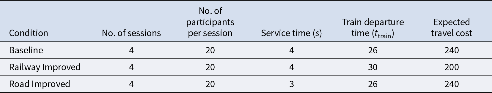
  $t^{\ast}=50$ (8:50), R = 500, α = 10, β = 5, and γ = 25. They differed in the values of service time (s) or train departure time (t train). Table 3 presents our experimental design. The effect of change in train departure time (i.e., travel time on the public route) was tested by comparing the Baseline and Railway Improved conditions. The effect of a change in service time was tested by comparing the Baseline and Road Improved conditions. The three conditions also differed from one another in the conversion rate of points into euros: $1200 = 1$ euro, $1300 = 1$ euro, and $1200 = 1$ euro for the Baseline, Railway Improved, and Road Improved conditions, respectively.
Experimental Design
Written instructions were handed to participants at the beginning of each session.Footnote 9 The instructions describe the bottleneck game as a simulation of the decisions faced by commuters traveling from a common origin to common destination each morning. Participants were informed that they would play 40 identical rounds, in each of which they would choose between traveling by car or by train. In the former case, they would travel on a road with a bottleneck characterized by a fixed service time and would select their departure time from the origin. In the latter case, they would travel by train, which departs at a predetermined time and arrives at the destination precisely at the desired arrival time  $t^{\ast}$. A numerical example illustrated the financial implications of choosing different departure times (see Table 1 in the instructions).
The payoff equations (see Section 2 above) were explained in detail and illustrated with a numerical example. To prevent negative cumulative payoffs (referred to as “bankruptcy”), each participant received an initial endowment of 10,000 points; tokens were added to or subtracted from this balance depending on the the payoff (positive or negative) earned in each round. Table 1 in the instructions is identical to Table 1 in the main text, except that it reports payoffs (R − C) rather than costs (C). The decision screen (Figure 1 in the instructions) displayed 60 alternative departure times. The outcome screen (Figure 3 in the instructions) showed the departure times of all group members, the participant’s payoff for the round, and their cumulative payoff. At the end of the session, participants were paid individually and dismissed. Excluding a common show-up fee of 2.50 euros, the mean payoffs in the Baseline, Rail Improved, and Road Improved conditions were 18.92, 18.76, and 19.23 euros, respectively.
5. Results
5.1. Aggregate behavior
Figure 2 presents side-by-side comparisons of the predicted, observed, and socially optimal cumulative relative frequency distributions of strategies, aggregated at the session level. The observed distributions were computed separately for rounds 1-10, 11-20, 21-30, and 31-40. In each panel, the thick line depicts the symmetric mixed-strategy equilibrium, whereas the thin lines represent the session-level distributions. In the Baseline and Railway Improved conditions, excess usage of the road persisted throughout the sessions. In the Road Improved condition, the observed distribution consistently remained within the area bounded by the equilibrium and socially optimal distributions, suggesting that car commuters spread out their departure times more than predicted, thereby alleviating congestion at the bottleneck. Thus, the observed behavior in the Road Improved condition lay between the equilibrium prediction and the social optimum, partially improving efficiency relative to equilibrium play, yet falling short of fully reaching the social optimum.
Predicted, observed, and socially optimal cumulative relative frequency distributions of strategies
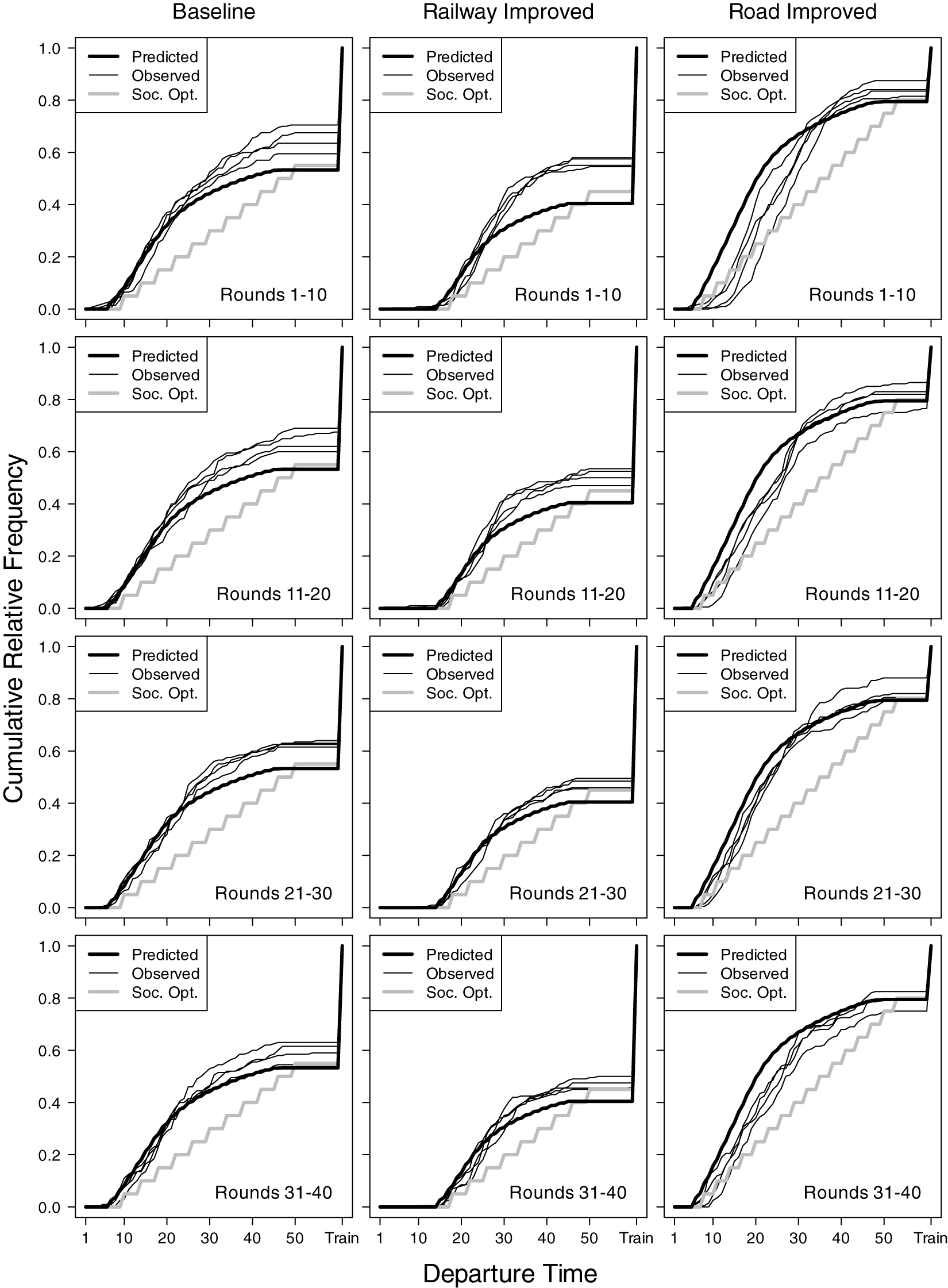
Visual inspection suggests that the observed distribution moved closer to the equilibrium distribution over time in each condition. We hypothesized that, as participants gained experience throughout the experiment, aggregate behavior would approach equilibrium play. To measure the distance between the observed and predicted distributions, we invoke the deviation index proposed by Stein et al. Reference Stein, Rapoport, Seale, Zhang and Zwick(2007) for each round:
 \begin{equation*}
DI_{jr}=\sqrt[]{\sum_{t\in T}\Big(p_{jrt}-p_{t}^{\ast}\Big)^{2}}
\end{equation*}
\begin{equation*}
DI_{jr}=\sqrt[]{\sum_{t\in T}\Big(p_{jrt}-p_{t}^{\ast}\Big)^{2}}
\end{equation*} where DIjr is the deviation index for session j in round r, pjrt is the relative frequency of departure choice  $t\in T=\{1,2,\dots,60\}\cup\{\text{Train}\}$ within session j in round r, and $p_{t^{\ast}}$ is the probability of choosing t under the symmetric mixed-strategy equilibrium.Footnote 10
We applied the one-sided Mann–Kendall trend test to assess whether the deviation index exhibited a decreasing trend over 40 rounds in each session. Each condition consists of four sessions, resulting in 12 independent trend tests. The results indicated a significant decreasing trend in 11 of the 12 sessions (p < 0.05). However, Session 2 (the second session in the Baseline condition) did not reject the null hypothesis ( $S = -26$, $Z = -0.291$, p = 0.385), suggesting no clear trend over the 40 rounds in that session.Footnote 11
Result 1.
Aggregate behavior approached equilibrium play with more experience.
Given that most sessions exhibit a decreasing trend in the deviation index, unless stated otherwise, we focus on the last ten rounds (rounds 31-40) for the remainder of the analyses. These rounds best reflect the participants’ more experienced decisions after the initial 30 rounds of play.
5.2. Testing the D-T hypothesis
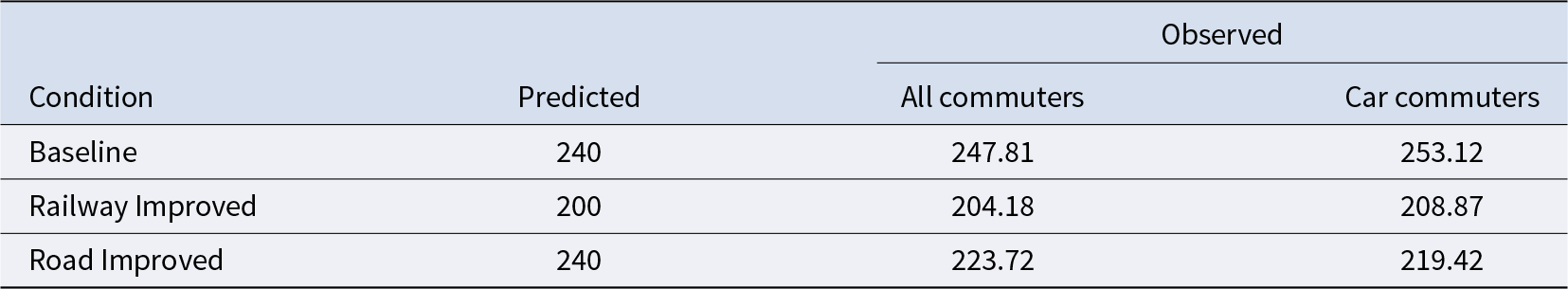
The D-T hypothesis posits directional predictions regarding mean travel costs; railway improvement reduces the mean travel cost, whereas road improvement leaves it unchanged. Table 4 reports the predicted and observed means of travel cost separately for all commuters (third column) and for car commuters (fourth column). The mean travel costs for all commuters were higher in the Baseline and Railway Improved conditions (247.81 versus 240 and 204.81 versus 200) and lower in the Road Improved condition than the equilibrium travel costs (223.72 versus 240). The data from the Road improved condition appeared to contradict the D-T hypothesis.
Predicted and observed means of travel cost (rounds 31-40)
To formally test whether our data support the D-T hypothesis, we estimated the following linear mixed-effects model with the Baseline condition as the reference group:Footnote 12
 \begin{equation}
\Delta\text{TC}_{it}=\beta_{0}+\beta_{1}\text{Railway_Improved}+\beta_{2}\text{Road_Improved}+r_{i}+r_{j[i]}+\epsilon
\end{equation}
\begin{equation}
\Delta\text{TC}_{it}=\beta_{0}+\beta_{1}\text{Railway_Improved}+\beta_{2}\text{Road_Improved}+r_{i}+r_{j[i]}+\epsilon
\end{equation} where 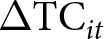 $\Delta\text{TC}_{it}$ represents participant i’s travel cost in round t minus the equilibrium travel cost for the reference group, namely 240. $\text{Railway_Improved}$ is a dummy variable taking the value of 1 if the condition is Railway Improved and 0 otherwise, and $\text{Road_Improved}$ is a dummy variable taking the value of 1 if the condition is Road Improved and 0 otherwise. ri is the random effect for player i, $r_{j[i]}$ is the random effect for session j in which player i participates, and ϵ is a general random term.Footnote 13 We expected an improvement of the railway to decrease and an improvement of the road not to change the travel cost, that is, $\beta_{1} \lt 0$ and $\beta_{2}=0$.
Table 5 presents the estimation results for Model (1). The estimated intercept is positive but insignificant. This indicates that participants in the Baseline condition incurred travel costs close to the equilibrium value of 240. The coefficient of Railway_Improved is negative and highly significant, consistent with the D-T hypothesis. However, the coefficient of Road_Improved is also significantly negative, contradicting the hypothesis that road improvements do not affect mean travel costs. Therefore, we confirm the evidence partially supporting our D-T hypothesis.
Result 2.
Contrary to the D-T hypothesis, not only railway improvement but also road improvement reduced the mean travel cost.
Estimation results for model (1)
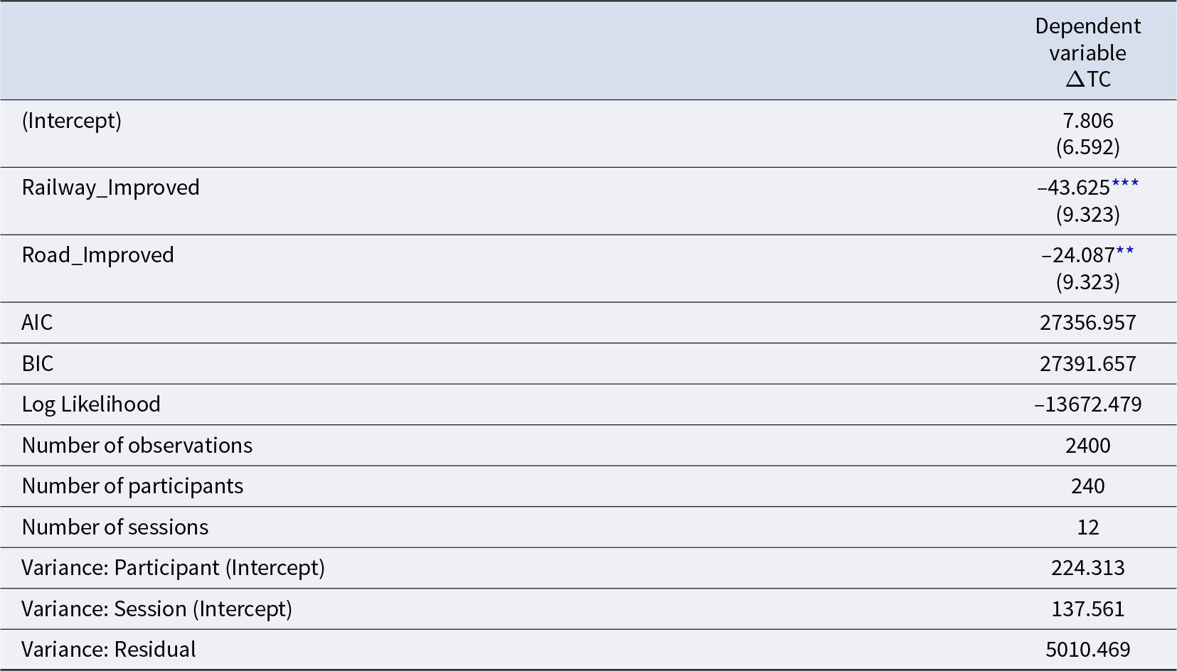
*** p < 0.001; **p < 0.01; *p < 0.05. Standard errors are in parentheses.
5.3. Behavior of car commuters
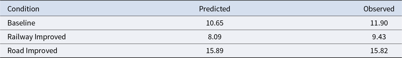
Table 6 presents the predicted and observed mean number of participants (out of 20) who traveled by car in each condition. Although the road was slightly overused in the Baseline and Railway Improved conditions, the observed means closely matched the symmetric mixed-strategy equilibrium predictions. However, the estimation results of Model (1) show that the observed mean travel cost was significantly lower than predicted not only in the Railway Improved condition but also in the Road Improved condition (see Table 5). Because the cost of traveling by train was fixed (240 in the Baseline and Road Improved conditions and 200 in the Railway Improved condition), the differences between the predicted and observed mean travel costs reflect only the behavior of car commuters. The fourth column of Table 4 shows the mean travel cost only for car commuters. The value is higher in the Baseline and Railway Improved conditions and lower in the Road Improved conditions than that for all commuters. Hence, car commuters are solely responsible for the increase in mean travel cost in the former two conditions and the decrease in the Road Improved condition.
Predicted and observed means of number of participants traveling by car (rounds 31-40)
How does the observed behavior of car commuters differ from equilibrium play? We compared the predicted and observed behavior of car commuters using four time-based metrics, departure time, waiting time, early arrival time, and late arrival time, as shown in Table 7. The predicted earliest and latest departure times correspond to those in the support of the symmetric mixed-strategy equilibrium.
Predicted and observed means of departure, waiting, early arrival, and late arrival times (rounds 31-40)
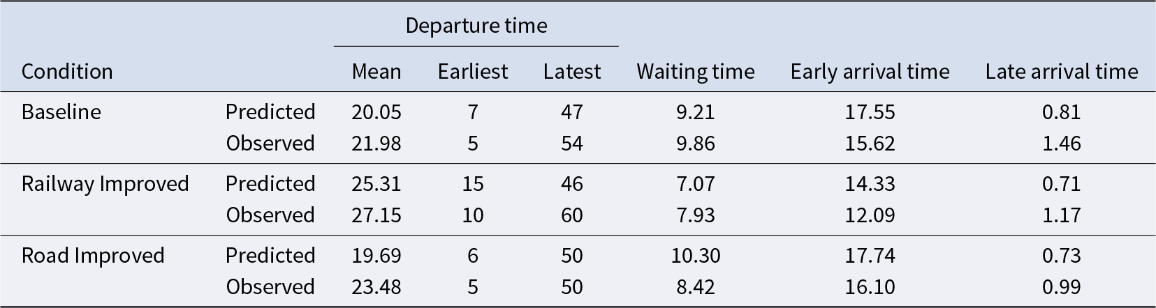
In all three conditions, car commuters tended to delay their departure times relative to equilibrium predictions. This pattern of delayed departures is accompanied by shifts in arrival patterns: the observed mean early and late arrival times are lower and higher than predicted, respectively, resulting in arrival times being shifted to later time slots.
Another discernible deviation concerns waiting time. In the Baseline and Railway Improved conditions, the observed mean waiting times exceeded the predicted ones, indicating that car commuters experienced more congestion than expected. In contrast, the observed mean waiting time is shorter than predicted in the Road Improved condition, suggesting that car commuters more effectively avoided queues at the bottleneck.
To formally test these patterns, we estimated the following intercept-only mixed-effects model for each time-based measure:
 \begin{equation}
\Delta_{it}=\beta_{0}+r_{i}+\epsilon
\end{equation}
\begin{equation}
\Delta_{it}=\beta_{0}+r_{i}+\epsilon
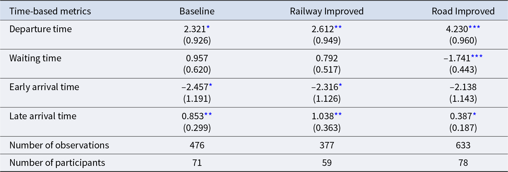
\end{equation} where  $\Delta_{it}$ denotes participant i’s observed time-based measure in round t minus the equilibrium value. This model evaluates whether the observed behavior systematically deviated from equilibrium predictions.Footnote 14 Table 8 presents the estimated intercepts of Model (2).Footnote 15 The intercepts for departure time are all significantly positive, confirming delayed departures in all three conditions. Therefore, we concluded the following result.
Result 3.
In all three conditions, car commuters departed later than predicted.
Estimated intercept of Model (2)
*** p < 0.001; **p < 0.01; *p < 0.05. Standard errors are in parentheses.
We also found that the intercepts for late arrival time were significantly positive in all conditions, whereas those for early arrival time were significantly negative in the Baseline and Railway Improved conditions. This pattern indicates an overall rightward shift in arrival times.
Result 4.
In all conditions, late arrivals occurred later than predicted. In the Baseline and Railway Improved conditions, early arrivals also occurred later than predicted.
In terms of waiting time, the observed mean waiting times were higher than predicted in both the Baseline and Railway Improved conditions, whereas the Road Improved condition exhibited a significant reduction in waiting time. This pattern was confirmed by the intercept-only mixed-effects model, where the only significant negative intercept was found in the Road Improved condition. Car commuters in the Road Improved condition, where the D-T hypothesis was not supported, appeared to tacitly coordinate their departure times to avoid unnecessary waiting at the bottleneck.
Result 5.
Car commuters in the Road Improved condition reduced their waiting times, whereas those in the Baseline and Railway Improved conditions did not.
The implications of Results 3-5 are reflected in the travel cost components summarized in Table 9. We added rows for the simulated results, which were generated from a reinforcement learning model calibrated using the experimental data (details provided in Section 6). In both the Baseline and Railway Improved conditions, car commuters experienced a decrease in early arrival cost and an increase in late arrival cost. These opposing effects offset each other, and the travel time cost remained close to the predicted values. Consequently, the observed mean travel costs in these two conditions were consistent with the equilibrium predictions.
Predicted, observed, and simulated means of travel cost and its components for car commuters (rounds 31-40)
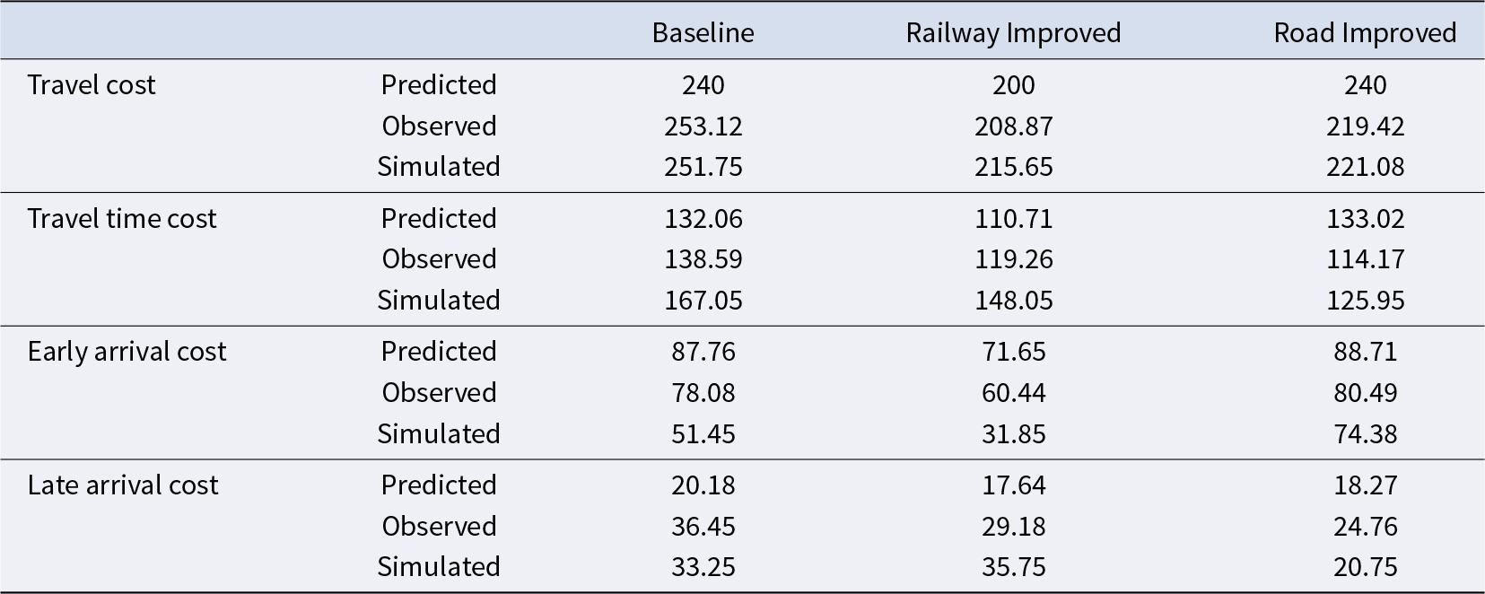
In contrast, the Road Improved condition showed a different pattern. In this condition, car commuters were able to avoid queues at the bottleneck, leading to a significant reduction in travel time cost. Although the mean late arrival cost increased, the gain from reduced travel time outweighed this increase. Consequently, the observed mean travel cost significantly fell below the predicted value.
5.4. Discussion
In our experiment, the D-T paradox predicted that improving the railway system (by reducing its travel time) should lower the mean travel cost, whereas improving road capacity (by reducing the bottleneck service time) should not affect the mean travel cost in equilibrium. Contrary to this theoretical prediction, our findings showed that both the Railway Improved and Road Improved conditions led to significant reductions in mean travel cost. In particular, car commuters in the Road Improved condition appeared to tacitly coordinate their departure times, thereby substantially reducing their waiting time at the bottleneck.
These results suggest that the D-T paradox did not fully manifest in our experimental setting. However, when isolating the mode choice dimension from the departure time dimension, the aggregate observed behavior was well accounted for by the equilibrium predictions (see Table 6). This pattern resonates with previous experimental studies on market entry games (Rapoport, Reference Rapoport1995, Sundali et al., Reference Sundali, Rapoport and Seale1995, Erev and Rapoport, Reference Erev and Rapoport1998, Rapoport et al., Reference Rapoport, Seale, Erev and Sundali1998), route choice games (Anderson et al., Reference Anderson, Holt, Reiley, Cherry, Kroll and Shogren2007, Selten et al., Reference Selten, Chmura, Pitz, Kube and Schreckenberg2007), and paradoxes in traffic networks (Morgan et al., Reference Morgan, Orzen and Sefton2009, Rapoport et al., Reference Rapoport, Kugler, Dugar and Gisches2009, Denant-Boèmont and Hammiche, Reference Denant-Boèmont and Hammiche2010, Dechenaux et al., Reference Dechenaux, Mago and Razzolini2014), which focus on choices among a small number of strategies, such as routes, modes, and markets. In these simpler settings, participants may be better able to coordinate equilibrium strategies, thereby giving rise to the paradoxical outcomes predicted by theory. In particular, studies on market entry games by Rapoport and colleagues (for example, Sundali et al., Reference Sundali, Rapoport and Seale1995, Erev and Rapoport, Reference Erev and Rapoport1998) have documented quick convergence toward equilibrium behavior. In contrast, although our participants’ aggregate behavior gradually moved closer to equilibrium over time (Result 1), it did not fully converge. In the Road Improved condition, in particular, the observed distribution of departure times consistently positioned itself between the equilibrium and the social optimum. This suggests a partial improvement in efficiency, deviating from the fundamental prediction of the paradox.
The departure from the D-T paradox may stem from the added complexity of our setting. Unlike route choice games or market entry games, our environment introduces a richer strategy space: participants choose not only whether to travel by car or train but also, if traveling by car, when to depart. Furthermore, the congestion externality caused by car commuters extends not only to those who choose the same departure time but also to those who depart later. This intertemporal spillover of the negative externality increases the difficulty of strategic coordination and may hinder convergence to the equilibrium outcomes consistent with the D-T paradox.
6. Learning
These findings indicate that equilibrium reasoning alone may not fully account for the observed behavior, raising the possibility that participants adapted through experience-based processes. To explore this idea, this section examined whether a simple reinforcement learning model could replicate the observed behavior at the aggregate level. Our model was a two-parameter reinforcement learning model built on the framework of Erev and Roth Reference Erev and Roth(1998), with an additional mechanism for experimentation. Reinforcement learning has been widely applied in economic experiments to model how individuals adapt their strategies based on past experiences. In the context of mode and departure time choices, commuters reinforced successful decisions while occasionally experimenting with alternative options.
We began by examining how participants’ past outcomes shaped their subsequent decisions. Our goal was to ground the learning model in the observed individual behavior. Importantly, we did not aim to construct a general model of learning behavior. Instead, we sought to develop a simple, ad hoc reinforcement learning model that captured the key features of our participants’ behavior while remaining as parsimonious as possible.
6.1. Effects of previous outcomes on subsequent decisions
How did our participants adjust their strategies across the 40 rounds of play? In our experiments, at the end of every round, each participant was informed of their choice of transportation mode, departure time, travel time, arrival time, individual payoff, and the choices of transportation mode and departure time by their group members. This feedback coupled with their personal experience may have guided participants to learn the structure of the game, adjusting their choices over time, influencing which transportation mode to use, and if traveling by car, at what time to depart, in the next round.
An excess payoff is defined as the actual payoff minus the equilibrium payoff (260 in the Baseline and Road Improved conditions and 300 in the Railway Improved condition). Figure 3 illustrates how the sign of excess payoff in the previous round affected change in departure time. To construct this figure, we focused only on the group of participants traveling by car over two consecutive rounds. Since the experiment consisted of 40 rounds, excess payoffs were computed for rounds 1 to 39, and changes in departure time were calculated as the departure time in round t minus the departure time in round t − 1 for rounds 2 to 40 ( $t=2,\dots,40)$. Thus, each change in departure time corresponds to the excess payoff received in the previous round.
Effect of previous excess payoff on change in departure time

A positive (negative) change in departure time implies departing later (earlier) than the departure time in the previous round. Figure 3 shows that car commuters tended to explore departure times around the chosen one, and the degree of exploration appeared to be larger for a negative excess payoff than for a non-negative excess payoff. However, in the Road Improved condition, car commuters tended to shift toward earlier departure times than the chosen one after having a negative excess payoff. We examined how changes in departure time responded to the previous round’s excess payoff by estimating the following linear mixed-effects model:Footnote 16
 \begin{align}
\Delta \text{DT}_{it}=&\beta_{0}+\beta_{1}\text{Excess_Payoff}_{it-1}^{+} \nonumber \\
&+\beta_{2}\text{Railway_Improved}+\beta_{3}\text{Road_Improved} \nonumber \\
&+\beta_{4}\text{Excess_Payoff}_{it-1}^{+}\times \text{Railway_Improved} \nonumber \\
&+\beta_{5}\text{Excess_Payoff}_{it-1}^{+}\times \text{Road_Improved} \nonumber \\
&+r_{i}+\epsilon
\end{align}
\begin{align}
\Delta \text{DT}_{it}=&\beta_{0}+\beta_{1}\text{Excess_Payoff}_{it-1}^{+} \nonumber \\
&+\beta_{2}\text{Railway_Improved}+\beta_{3}\text{Road_Improved} \nonumber \\
&+\beta_{4}\text{Excess_Payoff}_{it-1}^{+}\times \text{Railway_Improved} \nonumber \\
&+\beta_{5}\text{Excess_Payoff}_{it-1}^{+}\times \text{Road_Improved} \nonumber \\
&+r_{i}+\epsilon
\end{align} where  $\Delta \text{DT}_{it}$ is player i’s departure time in round t minus her departure time in round t − 1, and $\text{Excess_Payoff}_{it-1}^{+}$ is a dummy variable taking the value 1 if player i’s excess payoff in round t − 1 is non-negative.
The estimation results in the second column of Table 10 indicate that car commuters adjusted their departure times in response to past payoff outcomes. After receiving a negative excess payoff, car commuters in the Baseline and Railway Improved conditions tended to depart earlier in the subsequent round. This temporal adjustment was even more pronounced in the Road Improved condition: car commuters exhibited a stronger tendency to depart earlier. In contrast, after receiving a non-negative excess payoff, car commuters generally departed later, although these temporal adjustments were relatively modest in all three conditions and did not differ significantly between the Baseline and Railway Improved conditions.
Result 6. Car commuters adjusted their departure times based on their past payoff outcomes, departed earlier after a negative payoff, especially in the Road Improved condition, and modestly later after a non-negative payoff in all conditions.

How did outcomes in the previous round influence modal choice in the subsequent round? If a commuter receives a lower payoff from traveling by car than the sure payoff from traveling by train, they may be more inclined to switch to the train in the next round. To examine whether the probability of choosing the train depended on the excess payoff in the previous round, we estimated the following generalized linear mixed-effects model:
 \begin{align}
P_{it}^{\text{Train}}=&f(\beta_{0}+\beta_{1}\text{Excess_Payoff}_{it-1}^{+} \nonumber \\
&+\beta_{2}\text{Railway_Improved}+\beta_{3}\text{Road_Improved} \nonumber \\
&+\beta_{4}\text{Excess_Payoff}_{it-1}^{+} \times \text{Railway_Improved} \nonumber \\
&+\beta_{5}\text{Excess_Payoff}_{it-1}^{+} \times \text{Road_Improved} \nonumber \\
&+r_{i})
\end{align}
\begin{align}
P_{it}^{\text{Train}}=&f(\beta_{0}+\beta_{1}\text{Excess_Payoff}_{it-1}^{+} \nonumber \\
&+\beta_{2}\text{Railway_Improved}+\beta_{3}\text{Road_Improved} \nonumber \\
&+\beta_{4}\text{Excess_Payoff}_{it-1}^{+} \times \text{Railway_Improved} \nonumber \\
&+\beta_{5}\text{Excess_Payoff}_{it-1}^{+} \times \text{Road_Improved} \nonumber \\
&+r_{i})
\end{align} where  $P_{it}^{\text{Train}}$ is player i’s probability of traveling by train in round t, and $f(\cdot)$ denotes the standard logistic function. The third column of Table 10 summarizes the estimation results for Model (4). The coefficient of $\text{Excess_Payoff}_{it-1}^{+}$ is negative and highly significant, indicating that a non-negative excess payoff reduced the probability of traveling by train in the subsequent round. In the Road Improved conditions, this effect was even more pronounced: the interaction between $\text{Excess_Payoff}_{it-1}^{+}$ and the Road Improved dummy was significantly negative, suggesting that car commuters who earned a non-negative excess payoff in the previous round were even less likely to switch to the train.
Result 7.
Car commuters were less likely to switch to the train in the subsequent round after receiving a non-negative excess payoff. This effect was especially strong in the Road Improved condition.
6.2. Reinforcement learning model
To specify our reinforcement learning model, we follow the notations of Camerer and Ho Reference Camerer and Ho(1999). Let  $\pi_{i}\big(s_{i}(t),s_{-i}(t)\big)$ be commuter i’s payoff in round t where $s_{i}(t)$ and $s_{-i}(t)$ are commuter i’s strategy and the strategies chosen by all but i in round t, respectively. Let $\pi^{\ast}$ be the equilibrium payoff.
Assumption 1. Probabilistic Rule: Commuters select their strategy probabilistically based on accumulated attractions. Attraction is the perceived desirability of choosing a particular strategy. We denote commuter i’s attraction to strategy j in round t by  $A_{i}^{j}(t)$ and their probability of choosing strategy j in round t by $P_{i}^{j}(t)$. Then, each commuter selects strategy j in round t based on the following probabilistic choice rule:
 \begin{equation*}
P_{i}^{j}(t)=\frac{A_{i}^{j}(t-1)}{\sum_{k\in T}A_{i}^{k}(t-1)}.
\end{equation*}
\begin{equation*}
P_{i}^{j}(t)=\frac{A_{i}^{j}(t-1)}{\sum_{k\in T}A_{i}^{k}(t-1)}.
\end{equation*} Assumption 2. Initial Attractions: To model a situation in which commuters have no prior bias for specific strategies, initial attractions (i.e., attractions at t = 0) are assumed to be uniform over all strategies: for any  $j\in T$,
 \begin{equation*}
A_{i}^{j}(0)=\frac{Q}{|T|},
\end{equation*}
\begin{equation*}
A_{i}^{j}(0)=\frac{Q}{|T|},
\end{equation*} where Q is the strength of initial attraction and  $|T|$ is the number of strategies (60 departure times plus the train, i.e., 61 strategies in total). This assumption ensures that learning emerges purely from reinforcement.
Assumption 3. Updating the Rule of Attractions: At the end of each round, attractions are updated according to the following rule:
 \begin{equation*}
A_{i}^{j}(t)=A_{i}^{j}(t-1)+R_{i}^{j}(t),
\end{equation*}
\begin{equation*}
A_{i}^{j}(t)=A_{i}^{j}(t-1)+R_{i}^{j}(t),
\end{equation*} where  $R_{i}^{j}(t)$ denotes the reinforcement that commuter i attaches to strategy j in round t. The reinforcement function of our model incorporates spillover reinforcement (“experimentation”), meaning that when commuters select departure times and receive payoffs, they not only reinforce the chosen strategies but also adjust the attractiveness of nearby strategies.Footnote 17 This assumption is particularly important in experimental games with a large number of strategies such as ours (61 strategies) because, as Erev and Roth Reference Erev and Roth(1998) argue, “players will not (quickly) become locked in to one choice in exclusion of all others” (p.863).
To determine the form of the reinforcement function, we utilized the behavior observed in our experiment. Figure 3 illustrates how commuters adjusted their departure times in response to deviations between their payoffs and the equilibrium payoff in the previous round. There are two discernible patterns that emerged consistently across all conditions. First, after experiencing a non-negative excess payoff, commuters tended to explore departure times close to their previous choices. Second, after incurring a negative excess payoff, commuters exhibited a tendency to depart earlier, and this tendency was even stronger in the Road Improved condition. In response to these observed patterns, we assume that the reinforcement function takes different forms depending on the following three cases:
(a) $s_{i}(t-1)\in \{1,2,\dots,60\}$ and
$\pi_{i}\big(s_{i}(t-1),s_{-i}(t-1)\big)\geq \pi^{\ast}$
$s_{i}(t-1)\in \{1,2,\dots,60\}$ and
$\pi_{i}\big(s_{i}(t-1),s_{-i}(t-1)\big)\geq \pi^{\ast}$Commuter i who traveled by car in the previous round received a higher payoff than the equilibrium payoff (i.e., a non-negative excess payoff). The reinforcement commuter i attaches to strategy j in round t is given by
\begin{equation*}
R_{i}^{j}(t)=
\begin{cases}
\pi_{i}\big(s_{i}(t-1),s_{-i}(t-1)\big)\cdot e^{-g\big|j-s_{i}(t-1)\big|}&\text{for $j\in \{1,2,\dots,60\}$}\\
0&\text{for $j=\{\text{train}\}$}\\
\end{cases}
\end{equation*}where g determines the sensitivity to deviations, which controls how much commuters explore different departure times. This reinforcement function ensures that commuter i attaches the maximum reinforcement to the chosen departure time, and the reinforcement spills over to departure times near the chosen one with diminishing intensity.
(b)
$s_{i}(t-1)\in \{1,2,\dots,60\}$ and
$\pi_{i}\big(s_{i}(t-1),s_{-i}(t-1)\big) \lt \pi^{\ast}$Commuter i who traveled by car in the previous round received a lower payoff than the equilibrium payoff (i.e., a negative excess payoff). The reinforcement function is given by
\begin{equation*}
R_{i}^{j}(t)=
\begin{cases}
\Big[\pi^{\ast}-\pi_{i}\big(s_{i}(t-1),s_{-i}(t-1)\big)\Big]\cdot e^{-g\big|j-s_{i}(t-1)\big|}\cdot I_{j \lt s_{i}(t-1)}&\text{for $j\in \{1,2,\dots,60\}$}\\
\pi^{\ast}-\pi_{i}\big(s_{i}(t-1),s_{-i}(t-1)\big)&\text{for $j=\{\text{train}\}$}\\
\end{cases}
\end{equation*}where the term
$\pi^{\ast}-\pi_{i}\big(s_{i}(t-1),s_{-i}(t-1)\big)$ is the foregone payoff commuter i could have gained if she had chosen the train option, and
$I_{j \lt s_{i}(t-1)}$ is an indicator function that takes one if departure time j is earlier than
$s_{i}(t-1)$. Commuter i attaches the foregone payoff to the train option and also reinforces earlier departure times with diminishing intensity, in an attempt to avoid congestion.(c)
$s_{i}(t-1)=\{\text{train}\}$In this case, commuter i traveled by train in the previous round. They reinforce only the train option by adding the equilibrium payoff:
\begin{equation*}
R_{i}^{j}(t)=
\begin{cases}
0&\text{for $j\in \{1,2,\dots,60\}$}\\
\pi^{\ast}&\text{for $j=\{\text{train}\}$}\\
\end{cases}
\end{equation*}


6.3. Estimation and simulation
To estimate the two model parameters, Q and g, we employed the maximum likelihood estimation method. The estimation was perfomed separately for each experimental condition. Although the model was fit to the full data from rounds 1-40, the negative log-likelihood function was computed based only on the strategies observed in rounds 31-40. The parameter set that minimized the negative log-likelihood function was then identified for each condition: Q = 610.32 and g = 1.30 for the Baseline condition, Q = 550.77 and g = 1.32 for the Railway Improved condition, and Q = 949.57 and g = 1.22 for the Road Improved condition.
Following the estimation, the model was simulated for 100 iterations.Footnote 18 In each iteration, 20 simulated commuters played 40 rounds, and then we constructed a single cumulative distribution by aggregating their strategies across commuters during rounds 31-40. Figure 4 displays the 100 simulated cumulative relative frequency distributions of strategies alongside the predicted and observed distributions separately for each condition. Our learning model broadly reflects the observed patterns of excess road usage in the Baseline and Railway Improved conditions and delayed departures in the Road Improved condition.
One hundred simulated cumulative relative frequency distributions (rounds 31-40)

Table 9 offers a more detailed evaluation of model performance by comparing the simulated and observed means of travel cost and their components. Although the model approximates the observed mean travel cost in each condition, it does not fully replicate the underlying behavioral patterns of car commuters. The fit is less accurate at the component level: in particular, the model tends to overestimate travel time costs and underestimate early arrival costs in the Baseline and Railway Improved conditions. Nevertheless, the model performs relatively well in the Road Improved condition, where it closely reproduces both travel cost and its components.
The fact that our model fits the Road Improved condition better than the other two conditions highlights that behavioral patterns varied meaningfully across conditions. Given these differences, it may be overly ambitious to expect a single, simple learning model to account for all observed behaviors equally well. Our goal was not to develop a general, comprehensive model of learning across all environments, but rather to explore whether a parsimonious reinforcement learning model grounded in the experimental findings could replicate the key behavioral patterns observed in our experiment.
7. Conclusion
This study considers a novel scenario that combines elements of the D-T paradox with elements of queuing theory in the morning commute. Commuters face a choice of traveling by private car or train from a common origin to a common destination. Car commuters are also required to choose their departure times. They make these decisions independently and anonymously. Car travel is risky because of congestion, whereas train travel is not (non-congestible). Car commuters face a trade-off between the cost of travel time on the congested road and the cost of schedule delay at the destination. The schedule delay cost is due to the uncertainty of arrival time at the destination; commuters are charged a linearly increasing cost for arriving too early or too late. Similarly, the travel time cost for car commuters is linear in the time they wait before entering the bottleneck plus the fixed time of service. In contrast, the train departs from the origin and arrives at the destination exactly on time, and train commuters are only charged a fixed travel cost.
We considered three conditions, Baseline, Railway Improved, and Road Improved, that differed in either the duration of service time at the bottleneck or the train’s travel time. For each condition, we numerically derived a symmetric mixed-strategy equilibrium in this richer strategic environment that integrates both mode and timing choices. According to the D-T hypothesis, improving the train by shortening travel time should decrease mean travel cost, whereas improving the road by reducing service time should have no effect. We experimentally tested the D-T hypothesis in a controlled laboratory experiment with a between-subjects design. Following a period of learning, participants’ decisions in all three conditions approached, but did not fully match, equilibrium play.
Our study makes two main contributions to the literature. First, we provide a numerical characterization of equilibrium in a setting in which commuters must make both mode and timing decisions, offering a new environment to examine the D-T paradox. Second, we show experimentally that, although railway improvement reduces mean travel cost as predicted, road improvement also lowers mean travel cost, contrary to the paradox. These results identify a boundary condition for the D-T paradox: it may fail to emerge in environments where people face multi-dimensional decisions and complex externalities that unfold over time. While this paradox may hold in simpler, cognitively less demanding decision settings, its predictive power could weaken when people must coordinate both their mode and timing decisions in the presence of intertemporal congestion effects.
The deviations from equilibrium were systematic and most evident in car commuters’ departure times. In the Road Improved condition, participants delayed their departures and were better able to avoid queuing, resulting in a significant reduction in travel time costs. Our reinforcement learning model captured some of those efficiency-enhancing patterns; although the model performed relatively well in the Road Improved condition, it did not fully replicate the underlying patterns of behavior in the Baseline and Railway Improved conditions.
One possible interpretation of the observed deviation from equilibrium is that the added complexity of our environment, which makes coordination difficult, leads to more stochastic behavior. As shown in Figure 2, the observed distributions of departure times tend to deviate from equilibrium in the direction of the 45-degree line (not shown in the figure), which corresponds to random behavior. This shift toward randomness may increase efficiency in the Road Improved condition, as the observed distributions move closer to the socially optimal distribution. However, in the Baseline and Railway Improved conditions, the same pattern of deviation may reduce efficiency, as the observed distributions diverge from the social optimum. These results suggest that randomness is not universally beneficial; although it may mitigate congestion and improve outcomes in certain settings, it can also undermine efficiency when it pushes behavior away from socially optimal patterns. Future research could explore models that account for both payoff-sensitive choices and random variation.
Our scenario complements previous models of the morning commute proposed in the transportation literature in which commuters choose among multiple routes or modes. The major difference is that, in our model, only car commuters face uncertainty regarding their arrival times. Although the assumption that group members are symmetric aids analytical tractability, its empirical validity is questionable. Real-world commuters are known to differ in their attitudes toward risk; some may prefer the certainty of the train, whereas others may value the flexibility of choosing their own departure times and internalize schedule delay costs differently. In this context, future research could incorporate such individual differences into commuter behavior models.
In summary, we find that groups of symmetric commuters systematically deviated from equilibrium predictions, although their choices gradually approached equilibrium over time. This study highlights that complexity in commuters’ decision environments can weaken the emergence of the paradoxical outcomes predicted by theory. The D-T paradox holds under some conditions but tends to weaken when individuals must coordinate both mode and timing decisions under congestion that unfolds dynamically over time.
Supplementary material
The supplementary material for this article can be found at https://doi.org/10.1017/eec.2025.10025.
Data availability statement
The replication materials for this study are available at https://doi.org/10.17605/OSF.IO/R678H.
Acknowledgements
We would like to thank guest editor Professor Ido Erev and an anonymous referee for their careful review of the paper and for their constructive comments and suggestions. We would also like to thank the participants of the 2023 Asia-Pacific Economic Science Association Meeting in Seoul for their valuable feedback on an earlier version of this paper.
Finally, we would like to express our heartfelt appreciation and pay tribute to our esteemed co-author and beloved dissertation advisor, Prof. Amnon Rapoport, who passed away before this paper was submitted. Therefore, we take full responsibility for any remaining errors. As his students and friends, we owe him an immeasurable debt of gratitude for his unwavering support, invaluable guidance, and lasting friendships. In loving memory and with profound gratitude, we dedicate this work to his enduring legacy.
Funding
This study was financially supported by the Max Planck Society.
Conflict of Interest
The authors declare that they have no conflict of interest.


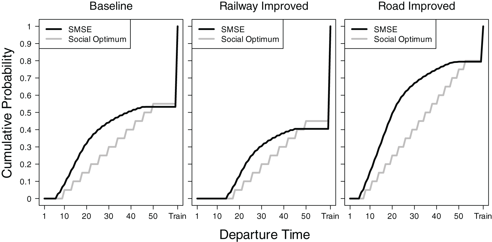


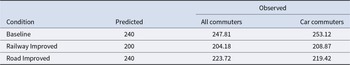

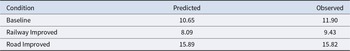
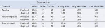

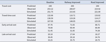
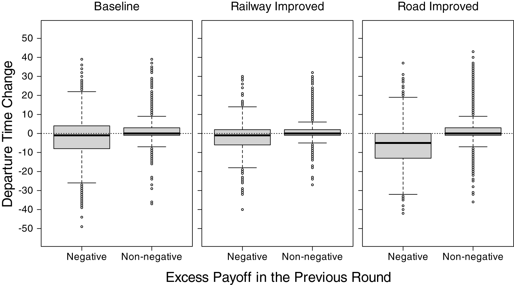


 Open access