


1. Introduction
Scholars debate how much campaigns, and events that take place during campaigns, matter for election outcomes (e.g., Holbrook, Reference Holbrook1996). The consensus is that typical campaign events like debates and speeches tend to have small effects on vote choice compared to “fundamentals” like voters’ economic perceptions and partisanship (e.g., Erikson and Wlezien, Reference Erikson and Wlezien2012; Sides and Vavreck, Reference Sides and Vavreck2013). By contrast, the limited literature on political scandals estimates substantial negative effects of scandals on support for candidates in U.S. House elections (e.g., Jacobson and Dimock, Reference Jacobson and Dimock1994; Welch and Hibbing, Reference Welch and Hibbing1997; Basinger, Reference Basinger2025). Importantly, scandals differ from traditional campaign events in that they often reveal previously unknown negative information about a candidate. Scandals are rare events that are hard to predict ahead of time, and it is therefore not surprising that there is limited information about the effect of scandals on support for presidential candidates. A more general question for researchers is how best to estimate the effects of realized scandals and forecast the effects of potential future scandals, as well as events more generally.
Cross-sectional academic studies, as well as most commercial polls, tend to measure the effect of events with a direct self-reported change question. These questions ask respondents to report how their attitude changed following a single event or would change if a future event took place (e.g., does [event X] make you more or less likely to vote for [candidate Y]?). Despite the ubiquity of this type of question, recent work has demonstrated its bias, with most questions yielding an exaggerated estimate of the extent to which an event (or learning about it, such as when a prior scandal is revealed) causes attitudes to change (Graham and Coppock, Reference Graham and Coppock2021). Graham and Coppock instead propose a novel counterfactual survey approach in which respondents predict their attitudes in the case that a future event either does or does not take place, or, if the event has taken place, to assess their attitude and, separately, what it would be if the event had not taken place. Importantly, in each scenario, respondents state an attitude given a state of the world, not a change in attitudes. For both cross-sectional methods, however, we lack an observational benchmark for assessing how effective they are at recovering estimates of attitude change observed from naturalistic stimuli (i.e., an event taking place) as well as clearly stated quantities of interest the methods seek to estimate.Footnote 1
In this paper, we compare the estimates from the change and counterfactual methods to a standard within-person panel estimate of the effect of an event taking place. The panel estimate shows how individuals’ attitudes change from before to after an event took place. Our first contribution is to formalize what this event study approach estimates and compare this estimate to the quantities estimated by the change and counterfactual methods. Importantly, we show that there are important conceptual differences in what each empirical approach estimates, which means differences across methodological approaches may be due to differences in what quantities of interest they are designed to estimate. We also apply each approach to the empirical question of how political scandals affect presidential vote choice. To do so, we utilize an eight-wave panel survey investigating Americans’ reactions to Donald Trump’s felony conviction in New York State on charges of falsifying business records to conceal hush money payments. Our panel is composed of a large number of respondents, was fielded both before and after the event of interest took place (conviction), and it includes both standard post-event change questions and pre-conviction counterfactual forecast questions following Graham and Coppock’s recommended approach.
After the guilty verdict was announced, the self-reported change question format yields estimates that Trump’s conviction affected a majority of the sample’s candidate support, especially among pre-existing Trump supporters. In particular, over 60% of Trump’s prior supporters report the conviction made them more likely to support him. The counterfactual question format yields an estimate in the opposite direction, suggesting that conviction decreased support by about 10 percentage points among existing supporters (compared to the state of the world in which he had been acquitted). Finally, our panel analysis, which measures change in individual-level support for the candidates from before to after the conviction, reveals that Trump’s conviction had almost no effect on any of his supporters, even among those who had previously indicated in response to the counterfactual item that their support was contingent upon his being found not guilty (acquitted).
We also demonstrate and characterize important analytic differences across these three estimators. In particular, both the event study approach, which is the estimate of what happens when an event takes place after accounting for expectations that it might take place, and the change format questions are affected by ex ante beliefs about the probability that an event might take place. They therefore answer the question of how opinions have changed once that uncertainty is resolved. By contrast, the counterfactual approach estimates a different quantity: the difference between the event not taking place and it taking place, where both states of the world are resolved with certainty. This answers the question of what the effect of one outcome is relative to another. Formalizing these estimators and the relationship between them is an important step for understanding several potential reasons they may produce different estimates and key analytic challenges in thinking more generally about how events (or information revelation) affect political outcomes. In light of these differences, it is particularly striking that the event study estimate of near-zero effect of the Trump conviction diverges sharply from the change format estimate.
Additionally, while the counterfactual forecast of the negative effect of Trump being found guilty (rather than not guilty) is closer to the (null) effect observed in the event study than the average positive effect estimated from the change question, it still substantially overestimates the magnitude of Trump’s conviction on vote choice. This is true even for those who indicated in response to the counterfactual questions that their support for Trump was conditional on his being found not guilty. It is also true for those who stated ex ante that they thought Trump would be found not guilty, for whom the event study estimate is closest to the counterfactual estimator because their pre-conviction opinion should reflect beliefs under the assumption Trump would be found not guilty. (As we show below, if one is certain an event will not happen ex ante, the quantity estimated by the counterfactual item is equivalent to the event study estimate.)
More generally, we highlight how estimating attitude change in both scholarly surveys and commercial polls is very difficult, particularly when surveys are cross-sectional (even if they utilize improved methods like the counterfactual format). Additionally, we show that campaign events, even an unprecedented one like Trump’s criminal conviction, appear to have minimal effects on presidential voters. Why even a criminal conviction does not change vote choice also has implications for our understanding of how voters choose between candidates in contemporary presidential races.
2. What do we know about campaign events?
Measuring the effects of events like these is a part of an extensive literature on the effect of events during election campaigns. In his 1996 book “Do Campaigns Matter?” Holbrook suggests that while campaigns can have short-term impacts on voter preferences, these shifts are often highly contextual, shaped by prevailing national conditions, which establish an equilibrium outcome that elections tend to reflect. Erikson and Wlezien (Reference Erikson and Wlezien2012) likewise find that “fundamentals” like economic perceptions and partisanship tend to dominate outcomes, and that campaigns essentially serve to reinforce pre-existing trends. Specific events like ads, speeches, and debates provide marginal adjustments compared to the role of fundamentals (Sides and Vavreck, Reference Sides and Vavreck2013), though they can potentially be pivotal (Vavreck, Reference Vavreck2009). Overall, scholars tend to agree that direct campaign efforts have minimal persuasive effects on changing voters’ candidate preferences. Where researchers do identify effects on vote choice, they are typically drawn from aggregated polling averages and lack precise estimation. Recent meta-analytical work concludes that campaign events are better equipped to mobilize supporters than lead to dramatic conversions in vote choice (Kalla and Broockman, Reference Kalla and Broockman2018).
In contrast to the scholarly consensus on campaign events, the effect of political scandals is less well studied at the presidential level. Jacobson and Dimock (Reference Jacobson and Dimock1994) identify an effect at the House level: the revelation that hundreds of House members had overdrawn their House-linked checking accounts led to the unusually high turnover of House seats in 1992. In another study, Welch and Hibbing (Reference Welch and Hibbing1997) find that charges of corruption against House incumbents lowers vote shares by nearly 10 percentage points (though “charges” in this case encompass a broad array of potential scandals). More recently, Basinger (Reference Basinger2025) likewise argues that House incumbents involved in a scandal tend to receive lower approval ratings and face lower likelihood of electoral support. Others find smaller declines in electoral support: some incumbents are hurt by scandals but able to recover by their next race if the scandal occurs early in their term (Brown, Reference Brown2006).
3. Asking about attitude change
The ideal measure of attitude change would be to use a panel, where the same respondents are interviewed immediately before and then immediately after an event to capture actual within-person change. Panel data are less vulnerable to recall bias, expressive responding, or forecasting issues that arise with cross-sectional measures. Using panel data, researchers can estimate the change in opinion from before to after an event. Importantly, opinion before the event might be influenced by expectations about the event occurring (such as if voters expect a scandal to occur), so the estimated treatment effect in the panel event study is the effect of learning the realized state of the world with certainty compared to existing uncertainty. As we discuss in detail below, the specific meaning of effects estimated from panel data has received little attention in the literature.
Despite the preferability of panel data, national polling organizations frequently try to estimate the effect of recent events using the “change format” of question.Footnote 2 In this cross-sectional question format, respondents are usually asked to reflect on how an event that has already taken place affected their choices. In the 2024 presidential election cycle, for example, many polling organizations sought to estimate the effect of different critical events on voters’ likelihood of supporting each candidate. Like estimates derived from panel data, this method seeks to estimate how attitudes have changed relative to existing opinion before an event, which can be influenced by prior expectations about the likelihood the event would occur in the future.
One such salient event was the verdict in Trump’s New York State criminal trial on charges of falsifying business records, a felony crime he was found guilty (convicted) of on May 30, 2024. To estimate the effect of this event on Trump’s support, a June 2024 poll conducted by the New York Times and Siena College asked, “Did Donald Trump’s conviction in the Manhattan hush money trial make you more likely to support him or less likely to support him, or did it make no difference in your support for him?” (NYT/Siena, 2024). While 19% of respondents indicated it made them “less likely to support him,” 68% said it “made no difference in support for him,” and 10% responded that conviction made them “more likely to support him.”
Overall, this pattern of response implies that the guilty verdict changed the level of support for Trump for 29% of voters. Under the assumption that increases and decreases in support were symmetric in magnitude and that individuals were reporting effects that were large enough to change their support for Trump, the difference between the increase and decrease support outcomes suggests the verdict resulted in a net 9 percentage-point decrease in support for Trump.
When restricting the sample to Republican voters, similar polls reveal an apparent increase in support for Trump. In one such poll conducted by Reuters and Ipsos on May 30–31, 2024, when asked how Trump’s recent conviction “… influenced your decision on whether or not to vote for [him] in the November election,” 34% of Republicans responded that it made them much or somewhat more likely to vote for him compared to 11% who responded much or somewhat less likely (Reuters-Ipsos Trump Guilty Verdict NY Hush Money Survey, 2024).
Past work, however, suggests these survey items that ask about changes in opinions may produce misleading estimates for a variety of reasons. For example, individuals may generally be poor at accurately recounting how a prior event affected their attitudes and behaviors (Watson, Reference Watson1924). Additionally, survey reports of changes may be affected by systematic measurement error. Gal and Rucker argue that survey respondents often answer questions in a manner that reflects other held attitudes or beliefs aside from those directly under study, which they call “expressive responding” (Gal and Rucker, Reference Gal and Rucker2011). In the context of attitude change, this approach suggests that respondents might express the intensity of their support rather than the change in it. Thus, the 10% of respondents reporting that Trump’s criminal conviction made them more likely to vote for him in the aforementioned poll could be signaling allegiance to Trump more so than reporting the actual effect of the conviction on their attitudes (but see Fahey, Reference Fahey2023 for evidence that expressive responding is rare). Other literature in this area further documents “expressive responding” in myriad partisan contexts (e.g., Yair and Huber, Reference Yair and Huber2021; Bullock et al., Reference Bullock, Gerber, Hill and Huber2015; Schaffner and Luks, Reference Schaffner and Luks2018).
To address the weaknesses of the change format questions, Graham and Coppock (Reference Graham and Coppock2021) instead propose a “counterfactual” format in which respondents are asked to report their attitude in two states of the world: if a treatment took place and if it did not. When these items are fielded prospectively (before an event took place), respondents are separately asked about their support specifying that the event does or does not take place. This order can be randomized, or different people can be randomly assigned to different conditions.Footnote 3 Subtracting a respondent’s “untreated” estimate from their post-treatment estimate is thus hypothesized to yield something closer to the causal effect of the treatment information on his or her attitudes. In the case of Trump’s federal indictment for the alleged mishandling of classified documents, Barari et al. (Reference Barari, Coppock, Graham and Padgett2024) find modest effects on vote choice using the counterfactual format, suggesting that the indictment slightly lowered Trump’s support among Republicans; by contrast, the change format produced “implausibly large” estimates that the indictment made Republicans more supportive of Trump.
The effect estimated by this method has a different meaning than those estimated by a panel or the change question. In the case of the counterfactual format, the estimate is not the change in opinion relative to prior opinion (which might be affected by uncertainty about the likelihood of the event occurring in the future). Instead, it is the difference in opinion between the event occurring with certainty and definitely not occurring. Because this estimand is fundamentally different than that of the other two methods, it affects how we should compare across estimates, which we explore in more detail in our discussion.
4. Data and methods
Our data are from a large-scale public opinion panel survey spanning the months before and after Trump’s conviction in his New York State criminal trial. These data were collected by YouGov and further details about the survey and sample demographics are available in the appendix. While the total sample includes approximately 130,000 respondents, we primarily rely on a panel of approximately 6,000 respondents who are re-interviewed monthly as part of a rolling 4-week cycle. We refer to these waves of the survey as “week 4” or “week 8,” for example, to make clear the time between interviews. The week 16 wave was fielded entirely before the announcement of Trump’s guilty verdict. The week 20 wave was in the field at the time of announcement and is thus subdivided into pre- and post-verdict periods where appropriate. All analyses are weighted using the weights provided by YouGov.
Our treatment of interest is Donald Trump being found guilty on 34 felony counts of falsifying business records on May 30, 2024. This took place while week 20 of our panel was in the field. We measured the effect of Trump’s conviction on vote choice using the change format:
Based on the result of the Manhattan trial, are you more or less likely to vote for Donald Trump for president in November? [Much more likely/Somewhat more likely/No effect/Somewhat less likely/Much less likely/Not sure]
Because the verdict interrupted our week 20 panel, we have this variable only for the subset of our whole weekly panel interviewed after the verdict was announced. Note that this is an estimate of the direction of an effect, while vote choice is categorical, meaning a respondent may be less (more) likely to vote for Trump without changing their vote.
We asked the counterfactual format item prospectively in week 16, prior to the conviction, with two questions that ask respondents to assess their voting in the presidential election in the event that Trump was found either guilty or not guilty.Footnote 4 We asked respondents both questions in a random order:
If Donald Trump is found guilty of falsifying business records, who would you vote for in November? [Joe Biden/Donald Trump/Someone else/Not sure/Will not vote in November]
If Donald Trump is found not guilty of falsifying business records, who would you vote for in November? [Joe Biden/Donald Trump/Someone else/Not sure/Will not vote in November]
Following Graham and Coppock’s approach, these prompts (1) explicitly describe the two potential treatment conditions (i.e., the outcome of Trump being found guilty or not guilty), (2) measure each respondent’s forecast vote choice in each conditions, and (3) allow estimation of the effect of being treated (found guilty) versus not (found not guilty) by calculating the difference in responses to the two questions. We use these data to identify two theoretically interesting types of potential Trump voters: “conditional” Trump voters, defined as those who indicated they would support Trump if he were found not guilty but would not support him if he were found guilty, and “unconditional” voters, defined as those who would support him regardless of the verdict.
We also adopt an event study approach using panel data to measure change in vote choice at the individual level using week 16 (pre-verdict) and week 20 vote choices. This is equivalent to a difference-in-differences approach with treatment determined by when respondents took the survey given that we have pre-treatment vote choice. We can also use vote choice measured in week 24 (and 16) to calculate estimates for all respondents.Footnote 5 The guilty verdict’s announcement during week 20 acts as our treatment, dividing survey respondents among those who responded before the announcement (our control group) and those who responded after the announcement (our treatment group).
Because the method proposed by Graham and Coppock identifies specific respondents whose vote choices are expected to change when uncertainty about an event is realized (i.e., Trump is found guilty), we can compare the estimates for this theoretically relevant subgroup to the estimates provided by the event study method with a triple-difference model. By definition, unconditional supporters should exhibit no change in vote intention before and after the verdict, while we would expect conditional voters to show a large decrease in support for Trump after the verdict, reflecting their stated conditionality in week 16 (i.e., they would support Trump only if he was not found guilty). We test how the verdict changed support among both groups below and compare these estimates to the estimates based on the retrospective and counterfactual formats.
5. Estimating the effect of campaign events
Because the survey in week 20 was interrupted by the guilty verdict, our data allow us to analyze a difference-in-differences model in Table 1. Approximately, 38% of the sample took the survey before the verdict was announced, and 62% took the survey after the verdict.
Linear regression of week 20 vote choice on post-verdict respondents, among week 16 Trump supporters with robust standard errors. Weighted analysis

Notes: Selected OLS coefficients with robust standard errors in parentheses. See Table A3 for complete results of the model with a control.
* p < 0.10, **p < 0.05, ***p < 0.01.
We regress respondents’ week 20 vote choice, among those who reported supporting Trump in week 16,Footnote 6 on whether they responded to our survey after Trump’s conviction was announced. (All analysis presented in this manuscript is weighted unless otherwise noted.) The difference-in-differences design thus compares vote choice of pre- and post-verdict respondents who supported Trump in week 16 (and who should not otherwise systematically differ before and after the verdict announcement). The pre-verdict difference is, therefore, 0 because all respondents supported Trump in week 16, and so this coefficient is omitted from the table. (As we explain above, theoretically this is the estimate of the effect of Trump being found guilty compared to attitudes when there was uncertainty about whether he would be found guilty and likely differences in those expectations.) Among this group of week 16 Trump supporters, we find no effect of taking the survey after the verdict was announced on vote choice. The coefficient is small (0.015) and not statistically significant (p > 0.05). These results appear in Table 1 and hold in an unweighted model (column 2) as well as one with controls (column 3).
5.1. Robustness
We test three key threats to inference in the appendix. First, we test the parallel trends assumption—both that late and early survey takers are usually the same in our panel and that our specific control and treatment groups are the same. We conduct a placebo test to show that later survey takers are not usually more or less likely to support Trump than early survey takers in column 1 of Table A4. Additionally, in Table A5, we show that our treatment and control groups do not differ in vote choice in weeks 4, 8, or 12. We also examined whether taking the survey post-verdict is associated with observable covariates. We regress whether a respondent took the survey post-verdict on observable demographic covariates in Table A6 and find few significant differences. Second, we look for evidence of differential non-response following the conviction. In column 2 of Table A4, we impute the vote choice of respondents who missed week 20 based on their next responses in weeks 24, 28, or 32. Third, we look for evidence of selection into treatment by instrumenting for survey response time by using past waves’ survey response time, in case respondents timed when they took the survey according to their views of Trump. We present the result of this instrumental variable approach in the final column of Table A4, where we find no evidence of differences among usual late and early survey takers.
Overall, the evidence supports the idea that there are no differences between the treatment and control group, either before or after Trump’s verdict. Across all methods of analyzing these data, there is no evidence that the conviction changed support among Trump supporters. We observe no evidence of differential attrition, selection, or differences among early and late survey takers that might confound this result.
6. Estimating campaign event effects using cross-sectional methods
6.1. Retrospective changes
Having established the null effect of the verdict using our event study approach, we next compare the estimates from our panel to the estimates from two cross-sectional methods. First, we consider the retrospective change question, which is often used to gauge the effect of campaign and news events on vote choice. We show that this measure correlates with contemporaneous measures of vote choice and also correlates with measures of change in vote choice constructed from our panel. However, the magnitude of reported changes in support vastly overestimates actual changes in candidate support and appears to reflect the fact that those voters who reported the verdict changed their vote were empirically, earlier in the campaign, highly variable Trump supporters, with similar week-to-week fluctuations in their wave-to-wave support for Trump as we observe after the trial verdict (i.e., they are simply “weak” Trump supporters).
In Table 2, we investigate the extent to which the change question reflects actual change in intended voting by comparing the retrospective change report to the event study estimate of actual changes in vote intentions. Thus, we benchmark the cross-sectional change item to the panel estimate. For simplicity, we continue to focus only on respondents who supported Trump in week 16 before the verdict was announced (following our difference-in-differences approach above, but see Table A7 for changes among the full sample).
Among week 16 Trump supporters, proportion supporting Trump in week 20 by how they reported the conviction changed their support. Weighted analysis

Note: Unweighted n = 1326. Regression estimates show that the only significant differences between groups are among “much less likely” (p < 0.1) and “much more likely” (p < 0.01) compared to the three intermediate categories.
Note the strong correlation between prior support for Trump and responses to the change item. Only 2.2% of prior Trump supporters said that the verdict decreased their support for him. Conversely, 60.5% of those who expressed support for Trump in week 16 report that the conviction made them much more likely to vote for him and he retains 99.6% of these votes. Only 0.2% of the sample reported that the conviction made them much less likely to vote for Trump, and 55.4% of this group actually shifted away. Interestingly, the patterns for the intermediate responses to the change item produce results that are not ordered as one might expect: Trump retains 90% of his supporters who said the verdict made them “Somewhat more likely” to support him but 92% of those who said it made them “Somewhat less likely” to do so. Overall, just 4.5% of week 16 Trump supporters shifted away from him post-verdict in week 20.
Taking the change item responses shown in Table 2 literally, it suggests a net positive gain among Republicans following the conviction. Since 89.3% of week 16 (pre-verdict) Trump supporters who said the verdict made “no change” in their support continued to support him in week 20, we can consider this Trump’s baseline retention rate. Table A8 shows that only the extreme categories are statistically different from this baseline. Among the small portion of the sample (0.2%) who reported that the verdict made them “much less likely” to support Trump, only 44.6% continued to support him. However, because this group is so small, the net impact is minimal: had conviction not occurred and Trump retained the same baseline 89.3% of the 0.2% subgroup, for example, the gain would have been negligible. However, Trump retains 99.58% of the respondents who report the conviction made them “much more likely” to support him (roughly 60.5% of the sample). This amounts to a 10 percentage-point increase in his retention rate compared to the “no change” group. Assuming that absent the verdict Trump would have retained support from 89.3% of this group, around 10% of this subgroup are additional supporters after the verdict (equating to approximately 6% of the full sample). This implies that the net result of Trump’s conviction is not a loss but a modest gain in support.
6.2. Counterfactual changes
Turning to our counterfactual measure of the impact of the guilty verdict, we find a much smaller number of Americans report that the verdict is important for their choice when asked in this way, and that the apparent effect is in the opposite direction (again restricted to week 16 respondents planning to vote for Trump).
Based on their responses to the counterfactual questions, we divide respondents into three groups: conditional Trump supporters who reported that their support for Trump was conditional on his being found not guilty (i.e., those who report they would vote for Trump if he were found not guilty but would not do so if he were found guilty), unconditional Trump supporters who said they would vote for him regardless of the trial outcome, and everyone who said they would not vote for him regardless of the trial outcome. In the appendix, we show that these categories roughly represent respondents who supported Trump regularly in our pre-trial panel waves (unconditional supporters), sometimes (conditional supporters), or extremely rarely (Table A9). In the appendix, we also demonstrate the demographic correlates of conditional support for Trump (Table A10). Table A10 shows that conditional supporters, compared to unconditional supporters, are more likely to have voted for another candidate in 2020 and more likely to be a Democrat who is supporting Trump. Overall, conditional Trump supporters appear to be weak Trump supporters.
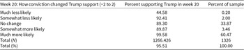
In Table 3, we divided week 16 Trump supporters into three groups based on their hypothetical vote choices. (The last group is composed of people who reported they would support Trump only if he was found guilty; we exclude those who said they would never support Trump, as they were not Trump supporters in week 16.) Among those who supported Trump in week 16, about 10% of respondents report they would not vote for him if he is found guilty. (In the full sample, 4.3% of respondents are conditional Trump supporters, while 35.9% are unconditional Trump supporters, and 59.8% accounts for everyone else.)
Classifying week 16 Trump supporters by their responses to the counterfactual forecast items. Weighted analysis

Note: Restricted to respondents who supported Trump in week 16, n = 2425.
7. Comparing the methods
The three methods produce substantially different answers. Our preferred difference-in-differences panel estimate is a null effect with a substantively small coefficient, while the change question format suggests a 6 percentage-point increase in support and the counterfactual question format suggests an 8–10 percentage-point decrease in support.
One explanation for these divergent results is that different methods, upon careful examination, estimate different underlying quantities. Graham and Coppock (Reference Graham and Coppock2021) specify a counterfactual in which all uncertainty over the outcome of an event is removed—the event either happened or did not happen. This differs from the change format in an important way, as the change format compares attitudes to before the event happened when there might have been uncertainty over the “true state of the world” (that is, whether an event would happen or had already happened).
Consider two related but distinct research questions about how events affect public opinion. The first—which we will call Question 1—asks how did an event change public opinion? This is the most commonly answered question in political science and public opinion research. It includes, for example, measuring shifts in vote choice after a scandal or changes in approval following policy implementation.
In this design, comparisons are typically drawn between attitudes before and after the event. However, pre-event attitudes already reflect expectations about the event’s likely outcome; indeed, political actors have beliefs about the probabilities that certain events will manifest (Huber, Reference Huber, Shapiro and Bedi2007). In our example, the trial’s effect will depend on whether it is a surprise to respondents. If a conviction is expected, the realization of the conviction might have no effect while if the conviction is unexpected the effect might be large. Thus, in practice, we often test the effect of an event relative to a baseline that includes uncertainty about its realization.
By contrast, a second question—Question 2—asks how would attitudes differ in a world where the event occurred compared to one in which it did not? This is a counterfactual question: it compares the real world to a specific hypothetical world in which the event never happened. In this framework, expectations are not part of the quantity of interest but rather noise that makes estimation harder. In our example, we look at the difference between guilty and non-guilty verdicts. Here, we are interested in the pure causal effect of the event turning out one way rather than the other, abstracted from prior expectations and uncertainty.
There are good reasons to be interested in both types of questions. For instance, in studying campaign scandals, Question 1 may be more relevant if we care about polling dynamics or the political returns to an action, while Question 2 may be more appropriate if we are focused on representation (e.g., are voters able to hold politicians to account?). Both questions are important, and researchers have developed tools for estimating each, even if the distinction between them is not always made explicit.
Below we define the answers to these questions formally. Before continuing, let us define a general notation for an observation of vote choice for individual  $i$ as ${Y_{ti}}\left( Z \right),{\text{ }}$ where $t \in \left\{ {0,1} \right\}$ measures time, denoting pre- (0) and post-treatment (1), and $z \in \left\{ {0,{p_i},1} \right\}$, denoting treatment status with $0 \leqslant {p_i} \leqslant 1$ denoting expectations over whether the treatment will occur (i.e., values in a state where treatment status is unclear).
We define the estimand corresponding to the first of these research questions as the event study estimand:
 \begin{equation}\begin{array}{*{20}{c}}
E=\frac{\sum\left[Y_{1i}(1)-Y_{0i}(p_{i})\right]}{N}
\end{array},\end{equation}
\begin{equation}\begin{array}{*{20}{c}}
E=\frac{\sum\left[Y_{1i}(1)-Y_{0i}(p_{i})\right]}{N}
\end{array},\end{equation}where  ${Y_{0i}}\left( {{p_i}} \right) = {p_i}{Y_{0i}}\left( 1 \right) + \left( {1 - {p_i}} \right){Y_0}i\left( 0 \right).{\text{ }}$ In this model, we assume that attitudes before an event occurs are equal to the weighted average of the attitude if the event takes place, ${Y_{0i}}\left( 1 \right),{\text{ }}$and attitudes if the event does not take place, ${Y_0}i\left( 0 \right)$, with the weights for these different treatment states the likelihood of each event taking place. Equation (1) estimand therefore formalizes the idea of changes in attitudes—it explicitly compares attitudes following treatment to those before treatment, with pre-treatment attitudes explicitly forming the counterfactual.
We define the second estimand more simply as the prospective counterfactual estimand:
 \begin{equation}W_{Pr}=\frac{\sum\left[Y_{0i}(1)-Y_{0i}(0)\right]}N,\end{equation}
where we elicit, at  $t = 0$, the unobserved counterfactuals. This can also be conceptualized as a retrospective counterfactual estimand ${W_R}$, substituting values at $t = 1$ for those at $t = 0$. Note that ${p_i}$ does not appear in this estimator because we specify with certainty whether an event has occurred or not and compare the outcome across these conditions.
We can rearrange these equations to show that the two estimands will be equal if the following condition holds:
 \begin{equation}\begin{array}{*{20}{c}}
{E - {W_{Pr}} = {Y_{1i}}\left( 1 \right) - {Y_{0i}}\left( 1 \right) - {p_i}\left[ {{W_{Pri}}} \right] = 0}
\end{array}.\end{equation}
\begin{equation}\begin{array}{*{20}{c}}
{E - {W_{Pr}} = {Y_{1i}}\left( 1 \right) - {Y_{0i}}\left( 1 \right) - {p_i}\left[ {{W_{Pri}}} \right] = 0}
\end{array}.\end{equation} This implies the two will be equal if there is both no time trend (i.e., the values, if treated, are the same before and after treatment) and  ${p_i}$ is 0 (i.e., the pre-treatment values are equal to the value if the treatment did not occur when pre-treatment people do not think it will occur).Footnote 7
The no-time-trend condition arises because the prospective version of  $W$ is based on values prior to the event, while the value of $E$ is established after treatment. If the actual difference in treated potential outcomes changes between these times, the two values will diverge. On the other side of the equation, ${p_i}$ will be 0 when the expected probability of the event occurring is 0. In this case, attitudes should not take the event into account whatsoever. Conversely, if ${p_i}$ is large (on average, or for certain respondents), the bias will be large. The combination of ${p_i}$ and ${W_{Pri}}$ further means that the two estimates will be particularly different if ${p_i}$ and ${W_i}$ are correlated (i.e., people who expect the event to occur have a large individual treatment effect).
7.1. Event study (panel) estimator
It is possible that  $E$ is directly observable, as both ${Y_{1i}}\left( 1 \right)$ and ${Y_{0i}}\left( {{p_i}} \right)$ are observed in the real world. The main challenge to this estimation, however, is the need to narrow the window of time between $t = 0$ and $t = 1$ to prevent confounding (from other events or time trends). We take advantage of our survey design by comparing attitudes among survey respondents immediately before and after the event; because we have an interrupted survey wave, we have a very narrow event window. Additionally, we can subtract prior attitudes of respondents to estimate a treatment effect that accounts for fixed differences between groups (i.e., if early and late survey takers are different in terms of education, age, or another demographic). The narrow event window accounts for time trends and the difference-in-differences approach accounts for fixed differences between treatment and control groups. Thus, we define the difference-in-differences estimator as:
 \begin{equation*}
{\hat E}=\frac{\sum\left[{y}_{1i}(1)-Y_{0i}(p_{i})| z_{i}=1\right]}{\left(n|z_{i}=1\right)}-\frac{\sum\left[{y}_{1i}(0)-Y_{0i}(p_{i})| z_{i}=0\right]}{\left(n| z_{i}=0\right)}
\end{equation*}
\begin{equation*}
{\hat E}=\frac{\sum\left[{y}_{1i}(1)-Y_{0i}(p_{i})| z_{i}=1\right]}{\left(n|z_{i}=1\right)}-\frac{\sum\left[{y}_{1i}(0)-Y_{0i}(p_{i})| z_{i}=0\right]}{\left(n| z_{i}=0\right)}
\end{equation*}7.2. The change estimator
The retrospective change question tries to ask respondents about  $E$ directly. Instead of measuring either ${Y_{1i}}\left( 1 \right)$ or ${Y_{0i}}\left( {{p_i}} \right)$, it does so by asking respondents to report the difference between their current and prior views. As with the event study estimator, it implicitly accounts for the effect of prior beliefs about the likelihood the event will take place in the future when individuals are asked to change how their attitudes changed from ${Y_{0i}}\left( {{p_i}} \right)$.
7.3. The counterfactual estimator
Finally, the counterfactual method tries to measure W by asking respondents to provide a guess as to their own  ${Y_{ti}}\left( 0 \right)$ and ${Y_{ti}}\left( 1 \right)$. We can label these forecasts $Y_t^{\text{*}}\left( 0 \right)$ and $Y_t^{\text{*}}\left( 1 \right)$ and estimate:
 \begin{equation*}
{\hat W}_{Pr}=\frac{\sum Y_{0i}^{*}(1)-Y_{0i}^{*}(0)}{n}
\end{equation*}
\begin{equation*}
{\hat W}_{Pr}=\frac{\sum Y_{0i}^{*}(1)-Y_{0i}^{*}(0)}{n}
\end{equation*} Importantly, note that in the counterfactual method when asking about  ${Y_{ti}}\left( 0 \right)$ the survey questions are designed to measure attitudes if the event does not take place, meaning not just that it has not yet taken place, but rather that it will not take place and any uncertainty about its future occurrence has been resolved negatively.
We discuss below how the differences in our three estimates can be reconciled based on the formalizations presented above. Again, we use a case where we could anticipate that an event, if it occurred, was going to take place between waves of a panel survey: the guilty verdict in Donald Trump’s trial on allegations of falsifying business records in Manhattan. Trump was found guilty, which allows us to estimate the effect of this outcome on support. (Had Trump been found not guilty we would have instead been able to measure the effect of him being found not guilty given prior uncertainty.)
Given Equation (3), we can compare our counterfactual and difference-in-differences estimates. Importantly, note that conditional Trump supporters, if we take them at their word, must have expected Trump to be found not guilty because, if they expected him to be found guilty, they would not have supported him in week 16. We therefore expect to see this group become significantly less supportive of Trump following the conviction (even if they do not move entirely from one extreme counterfactual to the other).Footnote 8
In Table 4, we estimate a triple-difference model to examine the difference in support for Trump before and after the verdict among conditional and unconditional supporters. If the counterfactual measure accurately identified how respondents would react to a guilty verdict, there should be no differences pre- and post-verdict for unconditional Trump supporters but a decrease in support of 1 unit (from intending to vote for Trump to not) for conditional supporters. Additionally, the effect of being a conditional Trump supporter should appear only after he has been found guilty.Footnote 9 Thus, in column 1 of Table 4, we interact when respondents took the survey (after the guilty verdict or not) with an indicator for their conditional Trump supporter status to predict binary week 20 vote choice.
Combined test and placebo tests of conditional Trump support on vote choice among week 16 Trump supporters with robust standard errors. Weighted analysis

Notes: Selected OLS coefficients with robust standard errors in parentheses. Differences between early and late survey takers in week 16 are 0 by construction as the sample is limited to respondents who intended to vote for Trump in week 16.
* p < 0.10, **p < 0.05, ***p < 0.01.
The small and insignificant coefficient for “Post-guilty verdict” shows unconditional Trump supporters were not moved by the guilty verdict. On average, conditional Trump supporters show a substantial decrease in support relative to unconditional Trump supporters (−0.286, p < 0.01), but this is the decrease in support before the verdict was announced.
Instead, the interaction between post-verdict response and conditional Trump supporter is the triple-difference estimate and is small and insignificant (p > 0.05), meaning that the gap between conditional and unconditional Trump supporters did not grow following the guilty verdict. This runs counter to what we would expect if conditional Trump supporters were accurately forecasting that their support for Trump (i.e., that they would vote for Trump if he were found not guilty and would not do so if he were found guilty). In the appendix, we further show that there is also no effect if we look only at Trump supporters who said they did not expect Trump to be convicted (see Table A11), a plausible proxy for ex ante beliefs about Trump’s likelihood of being convicted. These results also hold when we omit the survey weights (see Table A12).
Our data also allow us to use prior waves as a placebo test to make sure the differences (or lack thereof) are not due to differences in which respondents took the survey pre- and post-conviction. We can look at identical triple-difference estimates using outcome data from weeks 4, 8, and 12, to see if the estimates in week 20 appear substantively different from what we would expect when treatment did not occur. (We continue to define post-verdict using the timing of when the respondent took the week 20 survey.)
The remaining columns in Table 4 show the results of these placebo tests. We do not observe a significant difference between survey respondents who are unconditional Trump supporters and who, in week 20, took the survey before or after the verdict in any previous week. The coefficients for the effect of being in the post-guilty verdict group on vote choice are small and insignificant, ranging from 0.001 in week 4 to 0.02 in week 12 (p > 0.05). At the same time, the difference between conditional and unconditional Trump supporters remains consistently negative across all waves with statistically significant coefficients ranging from −0.137 to −0.291. The range of coefficients includes the week 20 coefficient, suggesting the pre-guilty verdict decrease in support was not an exceptionally large fluctuation. Instead, as we discuss above, conditional Trump supporters are simply weaker in the support for Trump across the whole survey period.
We note that the interaction term varies slightly across survey waves. In two of the weeks, the coefficients are small, positive, and insignificant (p > 0.05), while in week 4 it remains small and insignificant (p > 0.05) but negative. This shows that for conditional Trump supporters, the timing of their response to the week 20 survey is not correlated with differences in variability in Trump support.
It is useful to consider the amount of error in our week 20 estimate that would be necessary for this to be consistent with the counterfactual estimator. The constant in column 1 shows that the average support for Trump in week 20 (pre-verdict) is 0.944 among week 16 Trump voters. The main effect for conditional supporter status is −0.286 (p < 0.01), meaning that before the verdict support among conditional supporters was around 0.658 (0.944–0.286). Taking the counterfactual measure at face value we would expect Trump support in this group to drop to 0 post-verdict, meaning the interaction term would need to be about −0.658 to move post-verdict support to 0 among conditional Trump supporters. The actual coefficient, however, is 0.005, which is substantially smaller and in the wrong direction compared to the benchmark of −0.658. Even acknowledging the large standard errors on the estimated interaction effect, −0.658 falls well outside the 95% or even 99% confidence intervals.
We therefore conclude that the counterfactual estimate does not identify a group who responds as they say they will. Instead, the negative effect for conditional status across all waves in Table 4 suggests they are simply weaker supporters prone to defection, and that their stated conditionality may instead reflect the intensity of their support.Footnote 10 Table 4 demonstrates that the formal differences between estimators alone cannot explain the differences we observe. In other words, it is not that they are both correct and simply estimating different quantities. Rather, we find that the differences must emerge as a result of the cognitive process involved in providing accurate counterfactuals. Respondents do not provide accurate assessments of their own vote choice under hypothetical conditions.
In the appendix, we show that the null effect among conditional Trump supporters is robust to concerns over selection into treatment (see Table A13), differential attrition (see Tables A14 and A15), and to effects that might develop over time (see Figure A1).
We emphasize that the divergence between estimators is not just because they estimate different quantities of interest but also because each produces a fundamentally different empirical estimate of the effect of the event. The difference-in-differences estimate reflects actual behavior before and after the verdict was announced. The counterfactual format, by contrast, detects defection among weaker supporters already less likely to maintain their support for Trump. The differences reflect the differences between asking respondents to give hypotheticals and being able to measure actual change.
8. Discussion
Measuring attitude change is difficult and is a potential hurdle in identifying the effects of campaign events on American voters. In this paper, we provide evidence of a precisely estimated null effect of a major campaign event on vote choice—Trump’s conviction on 34 felony counts of falsifying business records. We argue that researchers studying these types of events have been studying two related questions: one estimating changes in public opinion and one comparing public opinion to specific unobserved counterfactuals. We formalize these estimates to demonstrate that these are distinct quantities of interest and then use our panel design to compare the answers to these two questions provided by cross sectional survey data. Empirically, we show that common methods that estimate attitude change from a single cross-sectional survey produce inaccurate estimates of effect sizes.
First, we estimate a difference-in-differences model using an interrupted wave of our panel where we compare attitudes of voters who had previously indicated they intended to vote for Trump just before and after the conviction. The change in intention to vote for Trump was small following the conviction (a 1.5 percentage-point increase) and not statistically significant. We compare this to the change format question asking respondents to self-report how the conviction changed their attitudes. This method has been used by many commercial pollsters and commentators; we show that it meaningfully overestimates effect sizes, and even direction, with 60% of Trump supporters stating the conviction increased their likelihood of voting for Trump. We calculate that this would equate to around a 6 percentage-point increase in support for Trump.
In response to these apparently implausible estimates, scholars have introduced a counterfactual question to address concerns about the change item approach (Graham and Coppock, Reference Graham and Coppock2021). This method answers the second question we describe above: it compares attitudes under a guilty verdict to attitudes under a counterfactual not-guilty verdict. The counterfactual estimate is an 8–10 percentage-point decrease in support for Trump. The difference between these estimates is not trivial: a null effect, a large increase, and a large decrease have very different implications for how the public responds to campaign events and scandals, as well as how campaigns should consider them.
To compare these estimates, we first carefully define the estimands that correspond to each method. We then estimate a triple-difference model, examining vote choice pre- and post-verdict among conditional (i.e., those who reported their support for Trump was conditional on his being found not guilty in the counterfactual format) and unconditional Trump supporters. The triple-difference estimate is small and insignificant, indicating the gap between conditional and unconditional Trump supporters did not grow after conviction. In other words, the counterfactual estimator does not correctly identify respondents whose support for Trump declined because of his guilty verdict.
Our unique ability to estimate a precise null in this case relies not only on our large panel design but its interruption by the event of interest in a very narrow window. We conclude that despite common measures indicating otherwise, political events, even when exceedingly rare, have little impact on voters’ attitudes (even though respondents may indicate otherwise). Our main result is consistent with the minimal effects consensus concerning campaign events. It also suggests that scandals at the presidential level, relatively understudied to this point, may also have little effect on voters. Because it is impractical to forecast campaign events and plan surveys around them (and as we note above, if this is possible then the estimate produced by the survey is not necessarily equivalent to the desired treatment effect if expectations are “priced in” already), our results are not meant to suggest the only way to measure campaign effects is to be lucky. Instead, we suggest researchers attend to the bias of their measures—when estimating an effect, do you capture an actual effect or an artifact of measurement (like response substitution, partisan cheerleading, or correlations between answers and another trait [like weak candidate support])?
Subsequent work should consider the extent to which survey instruments capture real world perceptions more broadly and in other contexts. In cases where attitudes are less crystalized, for example, are counterfactual estimates better predictors of real change? And can retrospective questions be useful measures of the direction of attitude shift, if not the magnitude? We hope future work continues to build on existing methods to understand when and where they are appropriate and what tradeoffs exist between cross-sections compared to panels.
Finally, while it somewhat beyond the scope of this paper, it is worth noting that the finding that even a criminal conviction has almost no effect on vote choice—even among people who say they did not expect it—is likely important evidence for understanding contemporary patterns of vote choice. This raises a broader question of whether this event—a conviction following a prosecution that some saw as partisan-motivated—is indicative of the difficulty of moving vote choice more generally or something about this specific event. With the tools and evidence provided in this paper we are in a better position to understand our ability to estimate the effect of this and related campaign events.
Supplementary material
The supplementary material for this article can be found at https://doi.org/10.1017/psrm.2026.10099. To obtain replication material for this article, https://doi.org/10.7910/DVN/VA0QPV.
Acknowledgements
We thank Alexander Coppock and Matthew Graham for helpful comments.


 Open access