





1. Introduction
Multi-tracer techniques show great promise in constraining primordial non-Gaussianity (PNG) when applied to next generation large-scale extra-galactic surveys. PNG encodes the dynamics of the early Universe and offers a sharp test of inflationary physics. In the widely used ‘local’ model (Bartolo et al. Reference Bartolo, Komatsu, Matarrese and Riotto2004; Chen Reference Chen2010), its amplitude is captured by $f_{\mathrm{NL}}$
, the fractional non-linearity, which imprints a distinctive, scale-dependent modulation of galaxy bias b on ultra-large scales k and at redshift z,
$f_{\mathrm{NL}}$
, the fractional non-linearity, which imprints a distinctive, scale-dependent modulation of galaxy bias b on ultra-large scales k and at redshift z, $\Delta b(k,z)\propto f_{\mathrm{NL}}\,k^{-2}$
(Dalal et al. Reference Dalal, Doré, Huterer and Shirokov2008; Reference Gomes, Camera, Jarvis, Hale and FonsecaGomes et al. 2020), enhancing power on the largest scales.
$\Delta b(k,z)\propto f_{\mathrm{NL}}\,k^{-2}$
(Dalal et al. Reference Dalal, Doré, Huterer and Shirokov2008; Reference Gomes, Camera, Jarvis, Hale and FonsecaGomes et al. 2020), enhancing power on the largest scales.
While attractor single-field slow-roll inflation predicts a nearly Gaussian field with $f_\mathrm{NL}\ll 1$
(Maldacena Reference Maldacena2003), non-attractor, or other non-standard dynamics can naturally yield
$f_\mathrm{NL}\ll 1$
(Maldacena Reference Maldacena2003), non-attractor, or other non-standard dynamics can naturally yield $f_\mathrm{NL}$
of order unity and distinctive bispectrum shapes (Bartolo et al. Reference Bartolo, Komatsu, Matarrese and Riotto2004; Chen Reference Chen2010). Current cosmic microwave background (CMB) bispectrum limits show no detection but still is consistent with local type non-Gaussianity
$f_\mathrm{NL}$
of order unity and distinctive bispectrum shapes (Bartolo et al. Reference Bartolo, Komatsu, Matarrese and Riotto2004; Chen Reference Chen2010). Current cosmic microwave background (CMB) bispectrum limits show no detection but still is consistent with local type non-Gaussianity $f_\mathrm{NL}^\mathrm{local}=-0.9\pm5.1$
(Planck Collaboration et al. Reference Collaboration2020), leaving room for further tests. Forecasts for upcoming surveys, for example with the SKA Observatory (SKAO) telescopes – the SKAO lowfrequency radio telescope (SKA-Low) and the SKAO mid-frequency radio telescope (SKA-Mid) – and with Euclid (Amendola et al. Reference Amendola2018), indicate sub-unity precision on
$f_\mathrm{NL}^\mathrm{local}=-0.9\pm5.1$
(Planck Collaboration et al. Reference Collaboration2020), leaving room for further tests. Forecasts for upcoming surveys, for example with the SKA Observatory (SKAO) telescopes – the SKAO lowfrequency radio telescope (SKA-Low) and the SKAO mid-frequency radio telescope (SKA-Mid) – and with Euclid (Amendola et al. Reference Amendola2018), indicate sub-unity precision on $f_\mathrm{NL}^\mathrm{local}$
under realistic assumptions, motivating a multi-tracer approach (Yamauchi et al. Reference Yamauchi, Takahashi and Oguri2014; Reference Gomes, Camera, Jarvis, Hale and FonsecaGomes et al. 2020).Footnote
a
$f_\mathrm{NL}^\mathrm{local}$
under realistic assumptions, motivating a multi-tracer approach (Yamauchi et al. Reference Yamauchi, Takahashi and Oguri2014; Reference Gomes, Camera, Jarvis, Hale and FonsecaGomes et al. 2020).Footnote
a
Multi-tracer methods are uniquely suited to this regime: by combining galaxy populations with different linear biases and redshift kernels, one can cancel cosmic variance in shared modes and convert relative clustering into information on $f_{\mathrm{NL}}$
. This typically involves identifying tracers of large scale structure which trace the underlying total matter distribution differently, and using the common distribution to negate the effects of cosmic variance. Large sky area surveys provide access to large angular scales, where the signals of non-Gaussianity are most likely to be found. Theoretical studies indicate we may be able to perform such techniques (Gomes et al. Reference Gomes, Camera, Jarvis, Hale and Fonseca2020; Ferramacho et al. Reference Ferramacho, Santos, Jarvis and Camera2014), where previously a lack of appropriately observed source populations, with identification of different tracers, has hampered efforts.
$f_{\mathrm{NL}}$
. This typically involves identifying tracers of large scale structure which trace the underlying total matter distribution differently, and using the common distribution to negate the effects of cosmic variance. Large sky area surveys provide access to large angular scales, where the signals of non-Gaussianity are most likely to be found. Theoretical studies indicate we may be able to perform such techniques (Gomes et al. Reference Gomes, Camera, Jarvis, Hale and Fonseca2020; Ferramacho et al. Reference Ferramacho, Santos, Jarvis and Camera2014), where previously a lack of appropriately observed source populations, with identification of different tracers, has hampered efforts.
Practical sensitivity depends on population mixing, relative ratios in clustering between active galactic nuclei (AGN) and star-forming galaxies (SFG), flux- and frequency-dependent selection, photometric-z errors, survey masks and depth gradients, resolution/morphology effects, and calibration systematics that can mimic large-scale power (Abramo & Leonard Reference Abramo and Leonard2013; Ferramacho et al. Reference Ferramacho, Santos, Jarvis and Camera2014; Gomes et al. Reference Gomes, Camera, Jarvis, Hale and Fonseca2020). A new, end-to-end forward simulation that ties halo populations, luminosity functions, and spectral assumptions to survey-specific observing effects is therefore essential to quantify biases, propagate uncertainties, and validate multi-tracer estimators in conditions that match real data.
Prior studies such as Bonato et al. (Reference Bonato2017) and the Tiered Radio Extragalactic Continuum Simulation (T-RECS) (Bonaldi et al. Reference Bonaldi, Bonato, Galluzzi, Harrison, Massardi, Kay, De Zotti and Brown2019) underpin our approach. Bonato et al. (Reference Bonato2017) matched redshift-dependent star formation rate (SFR) functions to 1.4-GHz radio luminosity functions (RLFs) to calibrate the radio-SFR mapping, explored linear vs. mildly non-linear relations (including scatter), updated the Massardi et al. (Reference Massardi, Bonaldi, Negrello, Ricciardi, Raccanelli and de Zotti2010) evolutionary model for radio-loud AGN, and used number counts to motivate a mild redshift evolution in the synchrotron/SFR ratio. T-RECS provides an end-to-end population synthesis for flat-spectrum radio quasars (FSRQ), BL Lac, and steep-spectrum AGN and for SFGs, including empirical/evolutionary RLFs, spectral-index prescriptions, size and subclass proxies, and mock catalogues designed to reproduce source counts and clustering. In this work, we adopt those physically motivated ingredients (RLF parameterisations, SFR to radio calibrations, and soft high excitation radio galaxies (HERG)/low excitation radio galaxies (LERG) mapping with mass weighting) but embed them in a halo-based framework tied to a cosmological lightcone (FLAMINGO; Schaye et al. Reference Schaye2023; Kugel et al. Reference Kugel2023) and a forward survey emulator. This lets us enforce consistency between RLFs and the halo supply via abundance matching and propagate realistic selection effects into counts, redshift distributions, and clustering – bridging population models and large-volume cosmology.
This study seeks to use N-body simulations and analytic halo population to verify the possibilities of using multi-tracer techniques in cosmology, with a realistic sky and experimental systematics. There will be two papers in this series: In this first paper we build the Galaxy Halo Occupation Simulation Tool (GHOST), an all-sky, clustered, survey-ready radio mock catalogue tied to a cosmological lightcone, expressly to validate multi-tracer pipelines for $f_\mathrm{NL}$
. We construct population- and survey-aware catalogues that reproduce wide-area measurements, quantify how selections reshape redshift kernels and deliver the calibrated inputs (galaxy positions, fluxes and halo mass mapping) required for end-to-end PNG tests. By supplying tracer families with distinct linear biases and redshift kernels, the catalogue enables controlled tests of cosmic-variance cancellation as it concerns non-Gaussianity constraints, estimator choices in configuration and harmonic space, and the impact of realistic masks, photo-z tails, and population misclassification (Seljak Reference Seljak2009; Abramo & Leonard Reference Abramo and Leonard2013; Ferramacho et al. Reference Ferramacho, Santos, Jarvis and Camera2014; Yamauchi et al. Reference Yamauchi, Takahashi and Oguri2014; Dalal et al. Reference Dalal, Doré, Huterer and Shirokov2008; Gomes et al. Reference Gomes, Camera, Jarvis, Hale and Fonseca2020; Planck Collaboration et al. Reference Collaboration2020).
$f_\mathrm{NL}$
. We construct population- and survey-aware catalogues that reproduce wide-area measurements, quantify how selections reshape redshift kernels and deliver the calibrated inputs (galaxy positions, fluxes and halo mass mapping) required for end-to-end PNG tests. By supplying tracer families with distinct linear biases and redshift kernels, the catalogue enables controlled tests of cosmic-variance cancellation as it concerns non-Gaussianity constraints, estimator choices in configuration and harmonic space, and the impact of realistic masks, photo-z tails, and population misclassification (Seljak Reference Seljak2009; Abramo & Leonard Reference Abramo and Leonard2013; Ferramacho et al. Reference Ferramacho, Santos, Jarvis and Camera2014; Yamauchi et al. Reference Yamauchi, Takahashi and Oguri2014; Dalal et al. Reference Dalal, Doré, Huterer and Shirokov2008; Gomes et al. Reference Gomes, Camera, Jarvis, Hale and Fonseca2020; Planck Collaboration et al. Reference Collaboration2020).
Paper 2 will use these products to perform the $f_\mathrm{NL}$
analysis on the simulated sky. The surveys of current instruments, such as the LoTSS; (LoTSS; Shimwell et al. Reference Shimwell2017) using the LOw-Frequency ARray (LOw-Frequency ARray (LOFAR); van Haarlem et al. Reference van Haarlem2013), as well as the planned surveys of future instruments like Euclid and the SKAO telescopes shall be used to inform source selection, identification and cosmological analysis, to predict the constraints that may be obtained on cosmological parameters.
$f_\mathrm{NL}$
analysis on the simulated sky. The surveys of current instruments, such as the LoTSS; (LoTSS; Shimwell et al. Reference Shimwell2017) using the LOw-Frequency ARray (LOw-Frequency ARray (LOFAR); van Haarlem et al. Reference van Haarlem2013), as well as the planned surveys of future instruments like Euclid and the SKAO telescopes shall be used to inform source selection, identification and cosmological analysis, to predict the constraints that may be obtained on cosmological parameters.
GHOST also will provide a simulation in the vein of T-RECS (Bonaldi et al. Reference Bonaldi, Bonato, Galluzzi, Harrison, Massardi, Kay, De Zotti and Brown2019) and Study Simulated Skies (SKADS) (Wilman et al. Reference Wilman2008), but with all-sky coverage as well as large-scale clustering. These improvements will support numerous cosmological applications, for example late-time CMB cross-correlation. Full-sky density fields with known selection allow pipeline development for the integrated Sachs–Wolfe effect and cross-correlation with CMB lensing convergence, including null tests under injected large-scale systematics (dipoles, depth gradients, bright-source masks) and validation of mitigation strategies using pseudo- $C_\ell$
machinery matched to survey footprints (e.g. Bahr-Kalus et al. Reference Bahr-Kalus, Parkinson, Asorey, Camera, Hale and Qin2022).
$C_\ell$
machinery matched to survey footprints (e.g. Bahr-Kalus et al. Reference Bahr-Kalus, Parkinson, Asorey, Camera, Hale and Qin2022).
Weak-lensing and magnification applications for GHOST are supported via add-on ray-tracing. Coupling the sky to a lensing engine (e.g. Borzyszkowski et al. Reference Borzyszkowski, Bertacca and Porciani2017, LIGER) turns the catalogue into a forward model for magnification and shear of radio sources, enabling tests of number-count and flux-weighted magnification estimators and of their sensitivity to the population mix and selection (Borzyszkowski et al. Reference Borzyszkowski, Bertacca and Porciani2017).
The GHOST simulation is also suited to studies of the cosmic radio dipole and survey-induced dipoles. With contiguous sky coverage and explicit selection functions, users can inject a kinematic dipole and survey systematics to quantify amplitude/direction bias, or measure the density dipole of flux-limited samples under controlled population mixtures. This connects directly to the radio-dipole literature (e.g. Böhme et al. Reference Böhme2025; Wagenveld et al. Reference Wagenveld, von Hausegger, Klöckner and Schwarz2025). For survey design, the large sky area of GHOST provides a sandbox for confusion, flux boosting, and spatially varying completeness. Because classes are labelled, the catalogue supports training and stress-testing of cross-identification and population-classification models under controllable class imbalance, and exploration of how selection affects downstream cosmology.
Finally, masking GHOST to medium/small fields enables direct forecasts of cosmic-variance floors and assessment of when multi-tracer or cross-correlation approaches deliver meaningful gains for deep tiers, while maintaining consistency with the wide-area selection and clustering that drive ultra-large-scale signals.
The subsequent Sections include a discussion of the FLAMINGO simulations (Schaye et al. Reference Schaye2023; Kugel et al. Reference Kugel2023) and how they were used here (Section 2), the model descriptions (Sections 3.2, 3.3, and 4) and results from the simulation in Section 5, including clustering (Section 5.3), redshift distributions (Section 5.6), source counts (Section 5.7), and RLF results (Section 5.8). The luminosity distribution with redshift is discussed in Section 6, and future improvements to GHOST in Section 7. We then finish with conclusions of the GHOST simulation in Section 8.
2. FLAMINGO simulation overview
The FLAMINGO simulations (Schaye et al. Reference Schaye2023; Kugel et al. Reference Kugel2023) comprise a suite of 28 runs – 16 hydrodynamical and 12 dark matter only (DMO) – spanning a range of particle numbers, particle masses, cosmological models, and box sizes. Developed by the Virgo Consortium, FLAMINGO aims to support upcoming large-scale structure surveys through high-fidelity predictions. The simulations use the SWIFT hydrodynamics code (Schaller et al. Reference Schaller2024), solving the fluid equations with the SPHENIX flavour of smoothed particle hydrodynamics (SPH) (Borrow et al. Reference Borrow, Schaller, Bower and Schaye2022). FLAMINGO features a novel approach to calibrating subgrid physics – including AGN feedback – by applying machine learning techniques trained on observed local datasets. Halo identification, whether in DMO or hydrodynamic simulations, was performed using the VELOCIraptor halo finder (Elahi et al. Reference Elahi, Cañas, Poulton, Tobar, Willis and Lagos2019). Subhalo properties were calculated using the Spherical Overdensity and Aperture Processor (SOAP) (McGibbon et al. Reference McGibbon, Helly, Schaye, Schaller and Vandenbroucke2025) code, developed specifically for FLAMINGO. Available data products include SOAP catalogues for multiple redshift snapshots, lightcones for select runs, and HEALPix maps of derived lightcone properties. The full FLAMINGO simulation specifications are detailed by Schaye et al. (Reference Schaye2023).
In this work, we use a FLAMINGO DMO simulation based on the best-fit cosmology from the Dark Energy Survey Year 3 analysis, specifically the ‘ $3\times2\mathrm{pt} + \mathrm{All\ Ext}\ \Lambda\mathrm{CDM}$
’ model. The corresponding cosmological parameters are listed in Table 1.
$3\times2\mathrm{pt} + \mathrm{All\ Ext}\ \Lambda\mathrm{CDM}$
’ model. The corresponding cosmological parameters are listed in Table 1.
We specifically use the L1000N3600 run, with a 1 Gpc $^3$
box and
$^3$
box and $3\,600^3$
particles of mass
$3\,600^3$
particles of mass $8.40\times10^8$
M
$8.40\times10^8$
M $_\odot$
, with the intention of providing sufficient mass resolution to resolve the halos of less massive, low SFR SFG.
$_\odot$
, with the intention of providing sufficient mass resolution to resolve the halos of less massive, low SFR SFG. $\sim$ $2.29\times 10^{9}$
halos were selected from a total of
$2.29\times 10^{9}$
halos were selected from a total of $\sim$ $1.14\times 10^{11}$
available in redshift
$1.14\times 10^{11}$
available in redshift $z=0$
to
$z=0$
to $z=10$
and assigned celestial coordinates (RA and Dec) based on their 3D positions in the simulation box at each redshift snapshot. The observer is located at (0, 0, 0), the centre of the coordinate system.
$z=10$
and assigned celestial coordinates (RA and Dec) based on their 3D positions in the simulation box at each redshift snapshot. The observer is located at (0, 0, 0), the centre of the coordinate system.
The FLAMINGO lightcone provides the two ingredients our $f_\mathrm{NL}$
tests are most sensitive to: ultra-large angular modes from a
$f_\mathrm{NL}$
tests are most sensitive to: ultra-large angular modes from a $\sim$
Gpc volume so that the lowest multipoles and cross-population covariance are realised in a single, contiguous sky; and a well-sampled halo mass function down to the scales that host low-SFR SFG. We intentionally anchor the abundance matching and host assignment to this specific halo field, because the PNG signal enters large-scale clustering primarily through the tracers’ (mass-dependent) bias. Using the same halo supply for catalog construction and for clustering predictions ensures that n(z), effective bias, and survey selections are mutually consistent when we calculate angular clustering statistics. While this paper employs a DMO run, baryonic effects are subdominant at the very large scales driving the scale dependent bias from non-Gaussianity; their residual impact is absorbed in the empirical validation against counts and n(z), and in the bias calibration we carry forward to Paper 2.
$\sim$
Gpc volume so that the lowest multipoles and cross-population covariance are realised in a single, contiguous sky; and a well-sampled halo mass function down to the scales that host low-SFR SFG. We intentionally anchor the abundance matching and host assignment to this specific halo field, because the PNG signal enters large-scale clustering primarily through the tracers’ (mass-dependent) bias. Using the same halo supply for catalog construction and for clustering predictions ensures that n(z), effective bias, and survey selections are mutually consistent when we calculate angular clustering statistics. While this paper employs a DMO run, baryonic effects are subdominant at the very large scales driving the scale dependent bias from non-Gaussianity; their residual impact is absorbed in the empirical validation against counts and n(z), and in the bias calibration we carry forward to Paper 2.
Cosmological parameters adopted for the fiducial flat $\Lambda$
CDM model used in this work. Columns list the symbol, parameter name, and adopted value (all quoted at
$\Lambda$
CDM model used in this work. Columns list the symbol, parameter name, and adopted value (all quoted at $\,z=0$
). We use the dimensionless Hubble constant h; the total matter, dark-energy, and baryon density parameters
$\,z=0$
). We use the dimensionless Hubble constant h; the total matter, dark-energy, and baryon density parameters $\Omega_{{m}}$
,
$\Omega_{{m}}$
, $\Omega_{\Lambda}$
, and
$\Omega_{\Lambda}$
, and $\Omega_{{b}}$
; the summed neutrino mass
$\Omega_{{b}}$
; the summed neutrino mass $\sum m_\nu$
; the amplitude and spectral index of the primordial scalar power spectrum,
$\sum m_\nu$
; the amplitude and spectral index of the primordial scalar power spectrum, $A_{{s}}$
and
$A_{{s}}$
and $n_{{s}}$
; and the present-day r.m.s. density fluctuation in
$n_{{s}}$
; and the present-day r.m.s. density fluctuation in $8\,h^{-1}\,\mathrm{Mpc}$
spheres,
$8\,h^{-1}\,\mathrm{Mpc}$
spheres, $\sigma_8$
. We also quote two derived parameters:
$\sigma_8$
. We also quote two derived parameters: $S_8 \equiv \sigma_8\sqrt{\Omega_{{m}}/0.3}$
and the neutrino density parameter
$S_8 \equiv \sigma_8\sqrt{\Omega_{{m}}/0.3}$
and the neutrino density parameter $\Omega_\nu$
defined via
$\Omega_\nu$
defined via $\Omega_\nu h^2 = \sum m_\nu/(93.14 \mathrm{eV})$
.
$\Omega_\nu h^2 = \sum m_\nu/(93.14 \mathrm{eV})$
.

3. Relation to T-RECS and rationale for a new implementation
Our goal is an all-sky, clustered, survey-ready radio mock catalogue built to validate multi-tracer pipelines on ultra-large scales and, ultimately, to constrain $f_\mathrm{NL}$
. This demands contiguous full-sky light-cones so that the lowest multipoles and cross-population covariances are realised, a halo assignment re-derived on our N-body field so that large-scale bias reflects the actual halo supply, and end-to-end, instrument-aware selection functions. T-RECS provides excellent population prescriptions and public clustered mocks, but its clustered realisations are limited in area and tied to a different halo pipeline, which is sub-optimal for the variance-cancellation regime targeted here (Bonaldi et al. Reference Bonaldi, Bonato, Galluzzi, Harrison, Massardi, Kay, De Zotti and Brown2019). For
$f_\mathrm{NL}$
. This demands contiguous full-sky light-cones so that the lowest multipoles and cross-population covariances are realised, a halo assignment re-derived on our N-body field so that large-scale bias reflects the actual halo supply, and end-to-end, instrument-aware selection functions. T-RECS provides excellent population prescriptions and public clustered mocks, but its clustered realisations are limited in area and tied to a different halo pipeline, which is sub-optimal for the variance-cancellation regime targeted here (Bonaldi et al. Reference Bonaldi, Bonato, Galluzzi, Harrison, Massardi, Kay, De Zotti and Brown2019). For $f_\mathrm{NL}$
, where the signal appears as a
$f_\mathrm{NL}$
, where the signal appears as a $k^{-2}$
modulation of bias at the largest angular scales, these constraints are decisive.
$k^{-2}$
modulation of bias at the largest angular scales, these constraints are decisive.
Population workflow used in GHOST. The diagram summarises how radio sources are generated for the two branches, with relevant subsections of the paper indicated by the bracketed numbers: SFG (left) and AGN (right). Green slanted boxes are external inputs (halo mass, redshift, base/other frequencies, external counts); cyan chevrons are operations/relations (e.g. SFR sampling, synchrotron/free–free relations, evolving RLF $\Phi(L)$
, spectral-index mapping, abundance matching); red rounded boxes are intermediate products or outputs (component luminosities
$\Phi(L)$
, spectral-index mapping, abundance matching); red rounded boxes are intermediate products or outputs (component luminosities $L_\mathrm{ff}$
/
$L_\mathrm{ff}$
/ $L_\mathrm{sync}$
, SFG/AGN luminosities, simulated counts, observer-frame fluxes). On the SFG side, sampled SFRs are converted to radio luminosity via synchrotron and free–free relations, then propagated to other frequencies. On the AGN side, type parameters (HERG/LERG, steep-spectrum AGN (SSAGN), etc.) and the evolving RLF (via
$L_\mathrm{sync}$
, SFG/AGN luminosities, simulated counts, observer-frame fluxes). On the SFG side, sampled SFRs are converted to radio luminosity via synchrotron and free–free relations, then propagated to other frequencies. On the AGN side, type parameters (HERG/LERG, steep-spectrum AGN (SSAGN), etc.) and the evolving RLF (via $L_\star$
and
$L_\star$
and $\Phi(L)$
) set the AGN luminosity, with spectral indices mapping to other bands. Both branches feed an abundance-matching step (using halo mass and redshift) to assign hosts and form the final matched-halo catalogue; the counts/interval-sum nodes provide predicted number counts used for verification. Arrows indicate data flow from inputs to catalogue outputs.
$\Phi(L)$
) set the AGN luminosity, with spectral indices mapping to other bands. Both branches feed an abundance-matching step (using halo mass and redshift) to assign hosts and form the final matched-halo catalogue; the counts/interval-sum nodes provide predicted number counts used for verification. Arrows indicate data flow from inputs to catalogue outputs.

We adopt the same high-level taxonomy and broad-band philosophy as T-RECS, and inherit some of the modelling: radio AGN split into FSRQ, BL Lacertae (BLLac), and SSAGN, and SFG with synchrotron and free–free contributions to their radio spectral energy distributions (Spectral Energy Distribution (SED)s). We retain smoothly evolving RLFs, class-dependent spectral-index distributions, and a minimalist Fanaroff–Riley (FR) proxy for internal labelling. GHOST differs from T-RECS in three ways most relevant to $f_\mathrm{NL}$
. First, we re-derive the luminosity-halo mapping against the FLAMINGO light-cone and use a rank-preserving, no-replacement match within each redshift slice; this enforces monotonicity, respects the available halo counts, and stabilises large-scale bias. Second, we generate contiguous, full-sky clustered realisations so the ultra-large angular modes are present. Third, our validation focuses on the observables that feed PNG analyses – Euclidean-normalised counts, redshift kernels n(z), and angular clustering
$f_\mathrm{NL}$
. First, we re-derive the luminosity-halo mapping against the FLAMINGO light-cone and use a rank-preserving, no-replacement match within each redshift slice; this enforces monotonicity, respects the available halo counts, and stabilises large-scale bias. Second, we generate contiguous, full-sky clustered realisations so the ultra-large angular modes are present. Third, our validation focuses on the observables that feed PNG analyses – Euclidean-normalised counts, redshift kernels n(z), and angular clustering $w(\theta)\!/C_\ell$
– for total and per-population samples under survey-like cuts. The stages of the simulation are shown in Figure 1.
$w(\theta)\!/C_\ell$
– for total and per-population samples under survey-like cuts. The stages of the simulation are shown in Figure 1.
For AGN, T-RECS draws host halo masses from HERG/LERG-based probabilities (inferred via stellar– to halo–mass relations) and associates each source to the nearest-mass halo in the same redshift slice, excluding already-assigned halos. For SFG, it fits an $L(M_h)$
relation by abundance matching and inverts it to map radio luminosities to halo masses, assigning those to halos per slice, with very faint sources below the halo–mass floor placed randomly on the sky. In GHOST we instead perform a global, rank-order match within each slice (monotonic
$L(M_h)$
relation by abundance matching and inverts it to map radio luminosities to halo masses, assigning those to halos per slice, with very faint sources below the halo–mass floor placed randomly on the sky. In GHOST we instead perform a global, rank-order match within each slice (monotonic $L\!\leftrightarrow\!M_h$
, no replacement), which prevents Eddington-style leakage across the steep end of the mass function, guarantees that the integral bias of each subsample matches the simulated halo supply, and reduces slice-to-slice bias fluctuations that would otherwise propagate into the
$L\!\leftrightarrow\!M_h$
, no replacement), which prevents Eddington-style leakage across the steep end of the mass function, guarantees that the integral bias of each subsample matches the simulated halo supply, and reduces slice-to-slice bias fluctuations that would otherwise propagate into the $k^{-2}$
PNG signature.
$k^{-2}$
PNG signature.
3.1. Types of galaxies in GHOST
GHOST includes four observational families that dominate the extragalactic radio sky at metre–centimetre wavelengths. Radio AGN appear in three classes – FSRQ, BLLac, and SSAGN – which differ in beaming/orientation and spectral behaviour but are often unified as the same central engine viewed at different angles (Urry & Padovani Reference Urry and Padovani1995; Heckman & Best Reference Heckman and Best2014). SFGs form a separate branch whose radio output tracks recent star formation. Below we summarise the properties and the labels used in this work.
-
• FSRQ: Flat-spectrum radio quasars show core-dominated, compact radio emission with flat spectra (assumed mean $\alpha=-0.1$
Footnote
b
), bright optical continua, and broad emission lines (Urry & Padovani Reference Urry and Padovani1995). In orientation-based unification they are relativistic jets viewed close to the line of sight, hence they have Doppler-boosted luminosities and are compact.
$\alpha=-0.1$
Footnote
b
), bright optical continua, and broad emission lines (Urry & Padovani Reference Urry and Padovani1995). In orientation-based unification they are relativistic jets viewed close to the line of sight, hence they have Doppler-boosted luminosities and are compact. -
• BLLac: Blazars with weak/absent emission lines and flat radio spectra, likewise interpreted as beamed (Doppler-boosted) jets at small inclination; compared to FSRQ they typically have lower line equivalent widths and similarly compact morphologies (Urry & Padovani Reference Urry and Padovani1995).
-
• SSAGN: Steep-spectrum radio AGN, representing the bulk of radio-loud AGN, with mean spectral index
$\zeta=-0.8$
. This class includes spectroscopic and morphological sub-taxonomies:-
– LERG: Jet-dominated systems with radiatively inefficient, low-Eddington accretion and weak/absent optical lines.
-
– HERG: Radiatively efficient (‘radiative-mode’) accretors with strong optical emission lines (Heckman & Best Reference Heckman and Best2014; Bonaldi et al. Reference Bonaldi, Bonato, Galluzzi, Harrison, Massardi, Kay, De Zotti and Brown2019).
-
– FR I: Edge-darkened morphology (brightness peaks nearer the core; jets fade outwards), more common at lower radio power (Fanaroff & Riley Reference Fanaroff and Riley1974).
-
– FR II: Edge-brightened lobes with terminal hotspots, more common at higher radio power (Fanaroff & Riley Reference Fanaroff and Riley1974).
-


These schemes probe different physics and are not one-to-one (e.g. FR II LERG exist). In our catalogue the FR tag is assigned via the size-ratio parameter $R_s$
(Section 3.3), defined as the separation of peak-brightness regions divided by the total source extent;
$R_s$
(Section 3.3), defined as the separation of peak-brightness regions divided by the total source extent; $R_s\gt0.5$
is labelled FR II and
$R_s\gt0.5$
is labelled FR II and $R_s\lt0.5$
FR I.
$R_s\lt0.5$
FR I.
-
• SFG: Radio emission powered predominantly by recent star formation: non-thermal synchrotron from cosmic-ray electrons accelerated in supernova remnants plus thermal free–free from H ii regions (Condon Reference Condon1992; Murphy et al. Reference Murphy, Chary, Dickinson, Pope, Frayer and Lin2011). At GHz frequencies the ensemble spectral index is steep (typ.
$\zeta\!\approx\!-0.7$
to
$-0.8$
) with a mild flattening from free–free towards higher frequencies. In GHOST the SFG branch is modelled with a calibrated RLF at 1.4 GHz and class-appropriate K-corrections; it is treated separately from AGN because its radio output traces star-formation physics rather than black-hole accretion.


Radio AGN typically inhabit more massive halos than SFG and therefore have a higher large-scale bias; within AGN, radiatively inefficient/jet-dominated systems tend to occupy the most massive environments, while radiatively efficient (quasar-like) systems are somewhat less clustered. Conversely, radio-selected SFG are associated with lower-mass halos and exhibit a lower bias. These trends are well-established in wide/deep radio clustering studies (e.g. Lindsay et al. Reference Lindsay2014; Magliocchetti et al. Reference Magliocchetti, Popesso, Brusa, Salvato, Laigle, McCracken and Ilbert2017; Hale et al. Reference Hale, Jarvis, Delvecchio, Hatfield and Novak2018) and are reproduced in our Section 5.3. The bias contrast between SFG and AGN is precisely the lever arm exploited by multi-tracer estimators; as such the presence of the trend in our simulation is of the upmost importance.
3.2. Star-forming galaxy radio luminosity function (SFG RLF)
We require an SFG description that is dust-insensitive and straightforward to propagate through survey selections across metre–centimetre bands. Rather than constructing an SFR function from UV/Infrared (IR) tracers and mapping $\mathrm{SFR}\!\to\!L_\nu$
, we calibrate the radio luminosity function of SFG directly at 1.4 GHz and model its smooth redshift evolution. This keeps the baseline independent of assumptions about obscured star formation and the IR-radio correlation, letting the radio data set the space density as a function of
$\mathrm{SFR}\!\to\!L_\nu$
, we calibrate the radio luminosity function of SFG directly at 1.4 GHz and model its smooth redshift evolution. This keeps the baseline independent of assumptions about obscured star formation and the IR-radio correlation, letting the radio data set the space density as a function of $L_\nu$
and z.
$L_\nu$
and z.
Relative to T-RECS, GHOST adopts a radio-derived baseline RLF for the SFG population, in which the 1.4 GHz RLF is fit directly and evolved smoothly with redshift. This reduces reliance on uncertain dust corrections and on the redshift evolution of the IR-radio correlation when setting the space density as a function of $L_\nu$
and z. The consequences of this modelling choice are quantified explicitly in Section 5.10, where an IR-calibrated construction and a thermal-dust SED extension are used as cross-checks. As discussed in Section 5.6, the radio-calibrated baseline tends to produce a smoother n(z) at fixed flux (less pronounced structure around
$L_\nu$
and z. The consequences of this modelling choice are quantified explicitly in Section 5.10, where an IR-calibrated construction and a thermal-dust SED extension are used as cross-checks. As discussed in Section 5.6, the radio-calibrated baseline tends to produce a smoother n(z) at fixed flux (less pronounced structure around $z\!\sim\!1$
-2) while preserving number counts and large-scale clustering.
$z\!\sim\!1$
-2) while preserving number counts and large-scale clustering.
For the functional form we adopt a smoothly broken (double-power-law) RLF with redshift-dependent normalisation and knee luminosity. All parameters are obtained by fitting to 1.4 GHz SFG RLF measurements in redshift slices, then validated against differential counts at 150 MHz (Franzen et al. Reference Franzen2016; Mandal et al. Reference Mandal2021), 1.4 GHz (Bondi et al. Reference Bondi, Ciliegi and Schinnerer2008; Bridle et al. Reference Bridle, Davis, Fomalont and Lequeux1972; Ciardi & Loeb Reference Ciardi and Loeb2000; Fomalont et al. Reference Fomalont, Kellermann, Cowie, Capak, Barger, Partridge, Windhorst and Richards2006; Gruppioni et al. Reference Gruppioni, Mignoli and Zamorani1999; Hopkins et al. Reference Hopkins, Afonso, Chan, Cram, Georgakakis and Mobasher2003; Ibar et al. Reference Ibar, Ivison, Biggs, Lal, Best and Green2009; Kellermann et al. Reference Kellermann, Fomalont, Mainieri, Padovani, Rosati, Shaver, Tozzi and Miller2008; Mitchell & Condon Reference Mitchell and Condon1985; Owen & Morrison Reference Owen and Morrison2008; Richards Reference Richards2000; Seymour et al. Reference Seymour2008; White et al. Reference White, Becker, Helfand and Gregg1997; de Zotti et al. Reference de Zotti, Massardi, Negrello and Wall2010) and 3 GHz (Smol $\breve{c}$
ić et al. Reference Smolčić2017) using the SFG spectral prescription applied elsewhere in this work. Fluxes at other frequencies are generated via standard K-corrections with that spectral model. The explicit evolution law and fitted coefficients are listed in Appendix A.
$\breve{c}$
ić et al. Reference Smolčić2017) using the SFG spectral prescription applied elsewhere in this work. Fluxes at other frequencies are generated via standard K-corrections with that spectral model. The explicit evolution law and fitted coefficients are listed in Appendix A.
In the multi-tracer context the SFG branch provides the lower-bias tracer with a broadly lower-redshift kernel set by the radio RLF and survey flux limit. Together with the higher-bias AGN branch this delivers the bias contrast and distinct P(z) kernels needed for cosmic-variance cancellation on ultra-large scales. Calibrating the SFG RLF directly in radio reduces sensitivity to dust-related systematics that could otherwise imprint spurious large-scale structure in n(z) and $w(\theta)$
, improving robustness for
$w(\theta)$
, improving robustness for $f_\mathrm{NL}$
forecasts.
$f_\mathrm{NL}$
forecasts.
3.2.1. Thermal dust SED term and IR-derived SFG RLF
The fiducial SFG population in GHOST is calibrated directly in radio (Section 3.2). Two additional ingredients are implemented as cross-checks and for multi-frequency completeness: an analytic thermal dust component in the SFG SED, and an IR-calibrated mapping that provides an alternative estimate of the effective $1.4\,\mathrm{GHz}$
space density. For multi-frequency catalogues, the radio SED is the sum of synchrotron and free-free components (Appendix A.6) and a thermal dust term is added,
$1.4\,\mathrm{GHz}$
space density. For multi-frequency catalogues, the radio SED is the sum of synchrotron and free-free components (Appendix A.6) and a thermal dust term is added,
 \begin{equation}{L_\nu^\mathrm{{SFG}}(\nu_\mathrm{rest})=L_\nu^\mathrm{sync}(\nu_\mathrm{rest})+L_\nu^\mathrm{ff}(\nu_\mathrm{rest})+L_\nu^\mathrm{dust}(\nu_\mathrm{rest}) .}\end{equation}
The dust term is modelled as a modified blackbody,
 \begin{equation}{L_\nu^\mathrm{dust}(\nu_\mathrm{rest})=A_{d}\,\nu_\mathrm{rest}^{\beta_{d}}\,B_\nu(\nu_\mathrm{rest},T_{d}),}\end{equation}
with fiducial $(T_{d},\beta_{d})=(45\,\mathrm{K},1.5)$
as adopted in the SKADS simulated skies (Wilman et al. Reference Wilman2008). The normalisation
$(T_{d},\beta_{d})=(45\,\mathrm{K},1.5)$
as adopted in the SKADS simulated skies (Wilman et al. Reference Wilman2008). The normalisation $A_{d}$
and the mapping between SFR,
$A_{d}$
and the mapping between SFR, $L_\mathrm{{IR}}$
, and
$L_\mathrm{{IR}}$
, and $L_{1.4}$
used in the verification are given in Appendix A.7.
$L_{1.4}$
used in the verification are given in Appendix A.7.
3.3. AGN population
For each class we adopt the T-RECS double-power-law RLF with smooth redshift evolution in normalisation and knee luminosity; the functional form is listed in Appendix A. Coefficients are refitted where required to remain consistent with the host assignment on our simulation and with the class mix used in this work; the resulting values and uncertainties are reported in Table 7. Observed flux densities at 150 MHz, 1.4 GHz, and 3 GHz are obtained from $L_\nu$
via standard K-corrections using class-dependent spectral-index distributions (flat for FSRQ/BLLac; steep for SSAGN), as in T-RECS. We do not model variability.
$L_\nu$
via standard K-corrections using class-dependent spectral-index distributions (flat for FSRQ/BLLac; steep for SSAGN), as in T-RECS. We do not model variability.
Sizes and a soft edge-brightening proxy are assigned to SSAGN to provide a morphology label used only for host weighting (Section A.4); this proxy is converted to a probabilistic HERG/LERG tag to allow overlap between morphology and excitation classes. Photometry is unaffected by these labels.
Hosts are assigned using the abundance-matching scheme defined in Section 4. In brief, AGN are matched to halos within redshift shells using a monotonic, no-replacement map, with class-dependent host probabilities and stellar-mass-weighted excitation fractions inspired by Janssen et al. (Reference Janssen, Röttgering, Best and Brinchmann2012). Tying the placement to our halo supply stabilises the large-scale bias of each class and ensures that the predicted $w(\theta)$
reflects the simulation’s actual halo population.
$w(\theta)$
reflects the simulation’s actual halo population.
Beamed subclasses are handled by drawing jet orientations isotropically and enforcing a maximum viewing angle per class and redshift to reproduce the observed beamed fractions. This yields flat spectra and compact sizes for the beamed subset while leaving the large-scale clustering unchanged.
In summary, we inherit the T-RECS class taxonomy, RLF functional form, and spectral prescriptions, while refitting the RLF coefficients where needed and replacing the original halo mapping with our abundance-matching scheme on the FLAMINGO light-cone.
4. Host assignment and abundance matching
All clustering results that follow use a host-assigned catalogue: every mock source is attached to a specific halo in the FLAMINGO DMO light-cone. We place this section before the clustering analysis to make explicit what catalogue underlies all $w(\theta)$
and
$w(\theta)$
and $C_\ell$
measurements.
$C_\ell$
measurements.
Given a survey selection, the requested number of sources in a $(\log L, z)$
bin is
$(\log L, z)$
bin is
 \begin{equation}\Delta N_{i,j} \;=\; \Omega \,\Phi(L\,|\,z_i)\,\left.\frac{dV}{dz}\right|_{z_i}\,\Delta\log L_{i,j}\,\Delta z_i ,\end{equation}
with $\Phi$
the class RLF (double-power-law with smooth evolution; see Appendix A). For SFG we realise these targets by fitting, per redshift slice i and flux density interval j, a monotone halo-to-luminosity map
$\Phi$
the class RLF (double-power-law with smooth evolution; see Appendix A). For SFG we realise these targets by fitting, per redshift slice i and flux density interval j, a monotone halo-to-luminosity map $L_\nu(M_h;\, z)$
(Equation 4) with optional log-normal scatter and then rank-ordering halos to luminosities without replacement. For AGN we first draw hosts with mass-weighted HERG/LERG properties (Appendix A), then assign
$L_\nu(M_h;\, z)$
(Equation 4) with optional log-normal scatter and then rank-ordering halos to luminosities without replacement. For AGN we first draw hosts with mass-weighted HERG/LERG properties (Appendix A), then assign $L_\nu$
monotonically within the selected subset to reproduce the class RLFs. When halos are scarce, we apportion the available hosts across populations in proportion to their requested counts (largest-remainder rule; Section 4.5) so the hosted mixture tracks the selection-driven requested mixture. This alignment of mixture, bias hierarchy, and selection is the key ingredient for robust multi-tracer
$L_\nu$
monotonically within the selected subset to reproduce the class RLFs. When halos are scarce, we apportion the available hosts across populations in proportion to their requested counts (largest-remainder rule; Section 4.5) so the hosted mixture tracks the selection-driven requested mixture. This alignment of mixture, bias hierarchy, and selection is the key ingredient for robust multi-tracer $f_\mathrm{NL}$
forecasts.
$f_\mathrm{NL}$
forecasts.
4.1. Assumptions and limitations
We assign a single central radio source per halo (no explicit satellites). The scatter $\sigma_{\log L}$
is taken to be constant within a shell. HERG/LERG labels are proxies for host-mass weighting rather than strict spectroscopic classes. At the highest redshifts, finite halo supply can saturate the brightest SFG targets; we quantify hosted versus requested counts in Section 5.8.
$\sigma_{\log L}$
is taken to be constant within a shell. HERG/LERG labels are proxies for host-mass weighting rather than strict spectroscopic classes. At the highest redshifts, finite halo supply can saturate the brightest SFG targets; we quantify hosted versus requested counts in Section 5.8.
4.2. Inputs and redshift shells
We partition redshift into disjoint shells: $\mathcal{Z}_i \equiv [z_i, z_{i+1}) \quad (i=0,$ $\dots, N-1),$
so that
$\dots, N-1),$
so that $\bigcup_{i=0}^{N-1}\mathcal{Z}_i = [z_0,z_N)$
and
$\bigcup_{i=0}^{N-1}\mathcal{Z}_i = [z_0,z_N)$
and $\mathcal{Z}_i\cap\mathcal{Z}_j=\varnothing$
for
$\mathcal{Z}_i\cap\mathcal{Z}_j=\varnothing$
for ${i\neq j}$
. (the same grid used for n(z) and RLFs). In each shell we compute the comoving shell volume per steradian and the target numbers per luminosity bin and population from the relevant RLF under the survey selection (cf. Equation 3). Candidate hosts are all halos in the shell, each with mass
${i\neq j}$
. (the same grid used for n(z) and RLFs). In each shell we compute the comoving shell volume per steradian and the target numbers per luminosity bin and population from the relevant RLF under the survey selection (cf. Equation 3). Candidate hosts are all halos in the shell, each with mass $M_h$
and light-cone position. We assign a stellar-mass proxy via the redshift-dependent
$M_h$
and light-cone position. We assign a stellar-mass proxy via the redshift-dependent $M_\star(M_h, z)$
relation of Aversa et al. (Reference Aversa, Lapi, de Zotti, Shankar and Danese2015).
$M_\star(M_h, z)$
relation of Aversa et al. (Reference Aversa, Lapi, de Zotti, Shankar and Danese2015).
4.3. SFG branch: Monotonic L–
$M_h$
abundance matching

For SFG we fit a smooth, monotonic mapping so that the host-assigned SFG luminosity histogram reproduces the radio SFG RLF $\Phi_\mathrm{{SFG}}(L_\nu, z)$
(Section 3.2). We adopt
$\Phi_\mathrm{{SFG}}(L_\nu, z)$
(Section 3.2). We adopt
 \begin{equation}L_\nu(M_h;\, z)\;=\;N(z)\,\Bigg[\Big(\frac{M_h}{M_\star(z)}\Big)^{\gamma}+\Big(\frac{M_h}{M_\star(z)}\Big)^{\beta}\Bigg]^{-1},\end{equation}
where $M_h$
is the halo mass, and
$M_h$
is the halo mass, and $M_*(z)$
,
$M_*(z)$
, $\gamma$
,
$\gamma$
, $\beta$
and N(z) are free parameters. with log-normal scatter
$\beta$
and N(z) are free parameters. with log-normal scatter $\epsilon\sim \mathcal{N}(0,\sigma_{\log L}^2)$
. The parameters
$\epsilon\sim \mathcal{N}(0,\sigma_{\log L}^2)$
. The parameters $\{N, M_\star, \gamma, \beta, \sigma_{\log L}\}$
are inferred independently in each shell by maximising a Poisson likelihood comparing the target counts (from the RLF) to the counts produced by rank-ordering halos in
$\{N, M_\star, \gamma, \beta, \sigma_{\log L}\}$
are inferred independently in each shell by maximising a Poisson likelihood comparing the target counts (from the RLF) to the counts produced by rank-ordering halos in $M_h$
and mapping to
$M_h$
and mapping to $L_\nu$
via Equation (4). We explore the posterior with an ensemble Markov-Chain Monte-Carlo (MCMC) (emcee, Foreman-Mackey et al. Reference Foreman-Mackey, Hogg, Lang and Goodman2013) and adopt median parameters for assignment.
$L_\nu$
via Equation (4). We explore the posterior with an ensemble Markov-Chain Monte-Carlo (MCMC) (emcee, Foreman-Mackey et al. Reference Foreman-Mackey, Hogg, Lang and Goodman2013) and adopt median parameters for assignment.
4.4. AGN branch: Mass-weighted host selection and monotone assignment
For radio AGN we draw hosts with a stellar-mass-dependent probability that encodes HERG/LERG tendencies and then assign luminosities monotonically within the selected subset so that the class RLFs are reproduced.
Each SSAGN is given a stochastic size from DiPompeo et al. (Reference DiPompeo, Runnoe, Myers and Boroson2013) and edge-brightening proxy $R_s$
from Lin et al. (Reference Lin, Shen, Strauss, Richards and Lunnan2010); we label
$R_s$
from Lin et al. (Reference Lin, Shen, Strauss, Richards and Lunnan2010); we label $R_s\gt0.5$
as FR II and
$R_s\gt0.5$
as FR II and $R_s\lt0.5$
as FR I and use this as a soft proxy for excitation class. Following Janssen et al. (Reference Janssen, Röttgering, Best and Brinchmann2012), ; Bonaldi et al. (Reference Bonaldi, Bonato, Galluzzi, Harrison, Massardi, Kay, De Zotti and Brown2019), we weight hosts by stellar mass, with a high-mass cap (‘saturation’) for the LERG branch:
$R_s\lt0.5$
as FR I and use this as a soft proxy for excitation class. Following Janssen et al. (Reference Janssen, Röttgering, Best and Brinchmann2012), ; Bonaldi et al. (Reference Bonaldi, Bonato, Galluzzi, Harrison, Massardi, Kay, De Zotti and Brown2019), we weight hosts by stellar mass, with a high-mass cap (‘saturation’) for the LERG branch:
 \begin{align}P_\mathrm{LERG}(M_\star|z)\;\propto\;\begin{cases}\left(M_\star/M_0\right)^{2.5}, & M_\star \le M_\mathrm{sat},\\[3pt]\left(M_\mathrm{sat}/M_0\right)^{2.5}, & M_\star \gt M_\mathrm{sat},\end{cases} \\[-25pt] \nonumber \end{align}
 \begin{align}P_\mathrm{HERG}(M_\star|z)\;\propto\;\left(\dfrac{M_\star}{M_0}\right)^{1.5},\end{align}
with $M_\mathrm{sat}\simeq 10^{11.6}$
M
$M_\mathrm{sat}\simeq 10^{11.6}$
M $_\odot$
. By ‘saturating’ we mean the LERG triggering weight stops increasing above
$_\odot$
. By ‘saturating’ we mean the LERG triggering weight stops increasing above $M_\mathrm{sat}$
. We renormalise
$M_\mathrm{sat}$
. We renormalise $P_t(M_\star|z)$
over candidate hosts in each redshift shell and draw hosts so that HERG/LERG totals match the RLF targets for that shell (FSRQ
$P_t(M_\star|z)$
over candidate hosts in each redshift shell and draw hosts so that HERG/LERG totals match the RLF targets for that shell (FSRQ $\rightarrow$
HERG-like; BLLac
$\rightarrow$
HERG-like; BLLac $\rightarrow$
LERG-like; SSAGN split by
$\rightarrow$
LERG-like; SSAGN split by $R_s$
). Hosts are sampled without replacement. Within each class and shell we sort hosts by
$R_s$
). Hosts are sampled without replacement. Within each class and shell we sort hosts by $M_h$
, sort luminosities by
$M_h$
, sort luminosities by $L_\nu$
, and map by rank (with optional log-normal L scatter) to reproduce the class RLF while anchoring large-scale bias to the actual halo field. FSRQ/BL Lac orientations are drawn isotropically (uniform in
$L_\nu$
, and map by rank (with optional log-normal L scatter) to reproduce the class RLF while anchoring large-scale bias to the actual halo field. FSRQ/BL Lac orientations are drawn isotropically (uniform in $\cos\theta$
).
$\cos\theta$
).
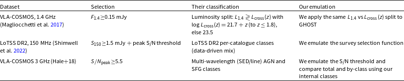
Classification schemes of comparison surveys and the emulation used in this work.
4.5. Population-weighted host apportionment
Let $\mathcal{L}_t(s)$
be the set of luminosities requested in slice s for population
$\mathcal{L}_t(s)$
be the set of luminosities requested in slice s for population $t\in\{\mathrm{FSRQ},\mathrm{BL\,Lac},\mathrm{SSAGN},\mathrm{SFG}\}$
, with size
$t\in\{\mathrm{FSRQ},\mathrm{BL\,Lac},\mathrm{SSAGN},\mathrm{SFG}\}$
, with size $R_t(s)=|\mathcal{L}_t(s)|$
. Let K(s) be the number of available hosts (unassigned halos) in the slice. If
$R_t(s)=|\mathcal{L}_t(s)|$
. Let K(s) be the number of available hosts (unassigned halos) in the slice. If $K(s)\ge R_\mathrm{tot}(s)\equiv\sum_t R_t(s)$
, all requests are hosted.
$K(s)\ge R_\mathrm{tot}(s)\equiv\sum_t R_t(s)$
, all requests are hosted.
When $K(s) \lt R_\mathrm{tot}(s)$
, we apportion the K(s) hosts across populations in proportion to requests using a largest-remainder rule:
$K(s) \lt R_\mathrm{tot}(s)$
, we apportion the K(s) hosts across populations in proportion to requests using a largest-remainder rule:
 \begin{align}q_t \;=\; \frac{R_t(s)}{R_\mathrm{tot}(s)}\,K(s), \qquad K_t \;=\; \min\bigl(R_t(s),\,\lfloor q_t\rfloor \bigr),\end{align}
then distribute the remaining $K(s)-\sum_t K_t$
one by one to populations with the largest fractional remainders
$K(s)-\sum_t K_t$
one by one to populations with the largest fractional remainders $q_t-\lfloor q_t\rfloor$
(never exceeding
$q_t-\lfloor q_t\rfloor$
(never exceeding $R_t$
). This guarantees
$R_t$
). This guarantees $\sum_t K_t=\min (K(s),R_\mathrm{tot}(s))$
and
$\sum_t K_t=\min (K(s),R_\mathrm{tot}(s))$
and $K_t\le R_t$
for all t.
$K_t\le R_t$
for all t.
Within each population, sort luminosities descending, $L_{t,(1)}\ge\cdots\ge L_{t,(R_t)}$
, and map rank to a host-mass index inside the quota via
$L_{t,(1)}\ge\cdots\ge L_{t,(R_t)}$
, and map rank to a host-mass index inside the quota via
 \begin{equation}i(r) \;=\; \Bigl\lceil r\,\frac{K_t}{R_t}\Bigr\rceil \in \{1,\dots,K_t\}.\end{equation}
Across all populations we collect these (predicted-mass, population) pairs, sort by predicted mass, and assign the top K(s) to the actual top K(s) halos (strictly preserving mass rank). Leftover requests $R_t-K_t$
are written as ‘no-halo’ rows (*NH) at the slice mid-redshift, preserving per-population totals and making host scarcity explicit.
$R_t-K_t$
are written as ‘no-halo’ rows (*NH) at the slice mid-redshift, preserving per-population totals and making host scarcity explicit.
4.6. Algorithmic summary
In each shell we compute target counts per class and luminosity bin from the relevant RLF (Equation 3) under the survey selection, gather all halos and assign $M_\star(M_h, z)$
from Aversa et al. (Reference Aversa, Lapi, de Zotti, Shankar and Danese2015), and then perform assignment by branch. For SFG we fit
$M_\star(M_h, z)$
from Aversa et al. (Reference Aversa, Lapi, de Zotti, Shankar and Danese2015), and then perform assignment by branch. For SFG we fit $L_\nu(M_h)$
via Equation (4) using an ensemble MCMC on a Poisson likelihood and assign by rank without replacement, adding log-normal scatter. For AGN we draw HERG/LERG hosts using
$L_\nu(M_h)$
via Equation (4) using an ensemble MCMC on a Poisson likelihood and assign by rank without replacement, adding log-normal scatter. For AGN we draw HERG/LERG hosts using $P_\mathrm{{HERG}/{LERG}}(M_\star)$
and, within each class, assign
$P_\mathrm{{HERG}/{LERG}}(M_\star)$
and, within each class, assign $L_\nu$
monotonically to match the class RLF. We then attach sky positions from hosts, apply spectral prescriptions and K-corrections, and finally apply the survey selection (flux/SNR survey selection functions and completeness surrogates).
$L_\nu$
monotonically to match the class RLF. We then attach sky positions from hosts, apply spectral prescriptions and K-corrections, and finally apply the survey selection (flux/SNR survey selection functions and completeness surrogates).
5. Initial results and catalogue validation
In this section, we present representative results from the simulated sky catalogue described above. We perform consistency checks against the input luminosity and redshift distributions, assess population statistics, and provide example sky visualisations. We will discuss applications to multi-tracer techniques. The simulated catalogue contains a total of $\sim$ $2.29\times10^{9}$
galaxies, comprising both AGN and SFG across
$2.29\times10^{9}$
galaxies, comprising both AGN and SFG across $4\pi$
steradians to a sensitivity of
$4\pi$
steradians to a sensitivity of $1\,\unicode{x03BC}\mathrm{Jy}$
at
$1\,\unicode{x03BC}\mathrm{Jy}$
at $1.4\,\mathrm{GHz}$
. The AGN population includes
$1.4\,\mathrm{GHz}$
. The AGN population includes $\sim$ $2.32\times10^{7}$
FSRQ,
$2.32\times10^{7}$
FSRQ, $\sim$ $2.08\times10^{7}$
BLLacs, and
$2.08\times10^{7}$
BLLacs, and $\sim$ $6.60\times10^{7}$
SSAGN, while the SFG population contributes
$6.60\times10^{7}$
SSAGN, while the SFG population contributes $\sim$ $2.18\times10^{9}$
sources. The redshift distribution spans the range
$2.18\times10^{9}$
sources. The redshift distribution spans the range $z \in [0, \sim6]$
, with the majority of sources concentrated below
$z \in [0, \sim6]$
, with the majority of sources concentrated below $z \sim 4$
.
$z \sim 4$
.
We use the same survey selections for both the redshift-distribution n(z) and clustering analyses to enable like-for-like comparisons with the literature. We re-classify for comparison with Magliocchetti et al. (Reference Magliocchetti2004) because the rule is a single, explicit luminosity threshold that can be mirrored exactly. We do not re-classify to compare with Hale et al. (Reference Hale, Jarvis, Delvecchio, Hatfield and Novak2018) because those clustering measurements treat the sample as a mixed population without a uniform AGN/SFG split. For a different reason, we do not re-classify for comparison with Hale et al. (Reference Hale, Jarvis, Delvecchio, Hatfield and Novak2018) because their labels are derived from multi-band diagnostics that are not available uniformly in our mock; we therefore emulate only the detection flux density threshold and separate population-mix effects (our classes) from selection effects (their S/N cut).
5.1. Selections used for validation
This Section defines the cuts and clarifies how each survey separated AGN from SFG (where they did), and how we mirrored those choices in GHOST. The three emulations are: the VLA-COSMOS 1.4 GHz luminosity threshold used by Magliocchetti et al. (Reference Magliocchetti, Popesso, Brusa, Salvato, Laigle, McCracken and Ilbert2017); the second data release (DR2) of LoTSS (Hale et al. Reference Hale2024; Shimwell et al. Reference Shimwell2022) wide-area 150 MHz flux and peak–S/N survey selection functions; and the VLA–COSMOS 3 GHz peak–S/N threshold and multi-wavelength classes of Hale et al. (Reference Hale, Jarvis, Delvecchio, Hatfield and Novak2018). Table 2 summarises the survey selection functions and our emulation strategy. As emphasised in Section 5.3, these selections compress or broaden the redshift kernel n(z) and thus reshape the projected clustering amplitude/slope without altering the intrinsic bias ordering, so we present raw and selected catalogues side by side in what follows.
Recent deep 1.4 GHz surveys with MeerKAT and the VLA (e.g. MeerKAT International GHz Tiered Extragalactic Exploration Survey (MIGHTEE); Jarvis et al. Reference Jarvis2016, GOODS-N; Owen Reference Owen2018) provide valuable constraints on the faint-flux population mix and redshift distributions. We do not adopt them as primary validation targets in this paper because our emphasis is on clustering with published two-point measurements. Nevertheless, as a consistency check in the $\unicode{x03BC}$
Jy regime, we also apply a MIGHTEE-like 1.4 GHz flux cut and inspect the resulting redshift distributions and class fractions in GHOST, finding the expected shift towards an SFG-rich sample while retaining a non-negligible AGN contribution at moderate redshift (e.g. Whittam et al. Reference Whittam2024).
$\unicode{x03BC}$
Jy regime, we also apply a MIGHTEE-like 1.4 GHz flux cut and inspect the resulting redshift distributions and class fractions in GHOST, finding the expected shift towards an SFG-rich sample while retaining a non-negligible AGN contribution at moderate redshift (e.g. Whittam et al. Reference Whittam2024).
5.1.1. LoTSS–DR2 wide 150 MHz
We emulate the LoTSS selection of (Shimwell et al. Reference Shimwell2022; Hale et al. Reference Hale2024) by combining an integrated-flux cut $S_{150}\ge 1.5\,\mathrm{mJy}$
with a peak–S/N threshold
$S_{150}\ge 1.5\,\mathrm{mJy}$
with a peak–S/N threshold $\mathrm{ S/N}_\mathrm{peak}\ge 7.5$
. This corresponds to a SFR of
$\mathrm{ S/N}_\mathrm{peak}\ge 7.5$
. This corresponds to a SFR of $\approx$ $6.7\times10^2$
M
$6.7\times10^2$
M $_\odot$
/yr. The image rms varies across the mosaic due to multiplicative effects, such as primary beam sensitivity, mosaicking overlap, and calibration/dynamic range, so we model the local rms
$_\odot$
/yr. The image rms varies across the mosaic due to multiplicative effects, such as primary beam sensitivity, mosaicking overlap, and calibration/dynamic range, so we model the local rms $\sigma$
as log-normal in an effort to replicate this,
$\sigma$
as log-normal in an effort to replicate this, $\ln\sigma\sim\mathcal{N}(\mu_{\ln},\sigma_{\ln}^2)$
. Anchoring the distribution to the median
$\ln\sigma\sim\mathcal{N}(\mu_{\ln},\sigma_{\ln}^2)$
. Anchoring the distribution to the median $\tilde{\sigma}=83\,\unicode{x03BC}\mathrm{Jy\,beam^{-1}}$
and 95th percentile
$\tilde{\sigma}=83\,\unicode{x03BC}\mathrm{Jy\,beam^{-1}}$
and 95th percentile $171\,\unicode{x03BC}\mathrm{Jy\,beam^{-1}}$
gives
$171\,\unicode{x03BC}\mathrm{Jy\,beam^{-1}}$
gives
 \begin{align}\mu_{\ln}=\ln\tilde{\sigma},\qquad\sigma_{\ln}=\frac{\ln\!(171 \unicode{x03BC}\mathrm{Jy})-\mu_{\ln}}{1.645}, \end{align}
which reproduces the observed quantiles by construction. For a source of integrated flux S (we take $S_\mathrm{peak}\!\approx\!S$
at 1.5 mJy; for resolved sources this is conservative), the S/N cut is equivalent to
$S_\mathrm{peak}\!\approx\!S$
at 1.5 mJy; for resolved sources this is conservative), the S/N cut is equivalent to $\sigma\le\sigma_\mathrm{thr}=S/7.5$
, yielding a detection probability
$\sigma\le\sigma_\mathrm{thr}=S/7.5$
, yielding a detection probability
 \begin{equation}p_\mathrm{keep}(S)=\Phi\!\left(\frac{\ln\sigma_\mathrm{thr}-\mu_{\ln}}{\sigma_{\ln}}\right),\end{equation}
with $\Phi$
the standard normal CDF. Using the class counts
$\Phi$
the standard normal CDF. Using the class counts $dN_X/dS$
, we define the area-weighted acceptances
$dN_X/dS$
, we define the area-weighted acceptances
 \begin{equation}\mathrm{acc}_X=\frac{\displaystyle \int_{S_{\min}}^\infty \frac{dN_X}{dS}(S)\,p_\mathrm{keep}(S)\,dS} {\displaystyle \int_{S_{\min}}^\infty \frac{dN_X}{dS}(S)\,dS},\qquad X\in\{\mathrm{SFG},\mathrm{AGN}\},\end{equation}
and form the effective mixture entering the total n(z),
 \begin{equation}w_\mathrm{{SFG}}=\frac{\mathrm{acc}_\mathrm{{SFG}}\,N_\mathrm{{SFG}}}{\mathrm{acc}_\mathrm{{SFG}}\,N_\mathrm{{SFG}}+\mathrm{acc}_\mathrm{AGN}\,N_\mathrm{AGN}},\end{equation}
where $S_{\min}=1.5\,\mathrm{mJy}$
and
$S_{\min}=1.5\,\mathrm{mJy}$
and $N_X$
are class totals from the un-gated n(z). At
$N_X$
are class totals from the un-gated n(z). At $S_{150}=1.5\,\mathrm{mJy}$
the flux threshold removes only a few percent of sources in both classes, so the resulting n(z) is dominated by the intrinsic SFG/AGN mix (Figure 9). Hale et al. (Reference Hale2024) does not supply a homogeneous AGN/SFG split for this clustering sample, so we emulate the selection only and compare the total n(z) and clustering; by-class predictions shown elsewhere use our internal labels to isolate population-mix effects from detection selection.
$S_{150}=1.5\,\mathrm{mJy}$
the flux threshold removes only a few percent of sources in both classes, so the resulting n(z) is dominated by the intrinsic SFG/AGN mix (Figure 9). Hale et al. (Reference Hale2024) does not supply a homogeneous AGN/SFG split for this clustering sample, so we emulate the selection only and compare the total n(z) and clustering; by-class predictions shown elsewhere use our internal labels to isolate population-mix effects from detection selection.
5.1.2. VLA–COSMOS 1.4 GHz
We mirror the flux density limit $S_\mathrm{1.4\,GHz}\ge 0.15$
mJy of Magliocchetti et al. (Reference Magliocchetti, Popesso, Brusa, Salvato, Laigle, McCracken and Ilbert2017) and re-classify sources using their redshift-dependent radio-luminosity boundary. This corresponds to a SFR of
$S_\mathrm{1.4\,GHz}\ge 0.15$
mJy of Magliocchetti et al. (Reference Magliocchetti, Popesso, Brusa, Salvato, Laigle, McCracken and Ilbert2017) and re-classify sources using their redshift-dependent radio-luminosity boundary. This corresponds to a SFR of $\approx$ $5.3\times10^2$
M
$5.3\times10^2$
M $_\odot$
/yr. Radio powers are computed as
$_\odot$
/yr. Radio powers are computed as $P_{1.4}=F_{1.4}\,D_A^2\,(1+z)^{3+\alpha}$
(W Hz
$P_{1.4}=F_{1.4}\,D_A^2\,(1+z)^{3+\alpha}$
(W Hz $^{-1}$
sr
$^{-1}$
sr $^{-1}$
) with
$^{-1}$
) with $\alpha=0.7$
and
$\alpha=0.7$
and $D_A$
the angular diameter distance, and the AGN/SFG division is
$D_A$
the angular diameter distance, and the AGN/SFG division is
 \begin{align}\log_{10} P_\mathrm{cross}(z)=\begin{cases}21.7 + z, & z\le 1.8 \nonumber \\[3pt]23.5, & z \gt 1.8\end{cases}\end{align}
(we convert to isotropic luminosity via $L_\mathrm{cross}=4\pi P_\mathrm{cross}$
). Objects with
$L_\mathrm{cross}=4\pi P_\mathrm{cross}$
). Objects with $L_{1.4}\ge L_\mathrm{cross}(z)$
are labelled ‘AGN-like’, the rest ‘SFG-like’. This reproduces their threshold classifier exactly and makes the comparison sensitive to population mix and redshift tails rather than to differences in detection survey selection functions; it also emphasises the overlapping mJy regime where both classes contribute (see Figure 10).
$L_{1.4}\ge L_\mathrm{cross}(z)$
are labelled ‘AGN-like’, the rest ‘SFG-like’. This reproduces their threshold classifier exactly and makes the comparison sensitive to population mix and redshift tails rather than to differences in detection survey selection functions; it also emphasises the overlapping mJy regime where both classes contribute (see Figure 10).
5.1.3. VLA–COSMOS 3 GHz
We emulate (Hale et al. Reference Hale, Jarvis, Delvecchio, Hatfield and Novak2018) catalogue’s peak-flux threshold $\mathrm{S/N}\ge 5.5$
with a field median rms
$\mathrm{S/N}\ge 5.5$
with a field median rms $\tilde{\sigma}\simeq 2.3\,\unicode{x03BC}\mathrm{Jy\,beam^{-1}}$
, modelling field-to-field rms as lognormal with
$\tilde{\sigma}\simeq 2.3\,\unicode{x03BC}\mathrm{Jy\,beam^{-1}}$
, modelling field-to-field rms as lognormal with
 \begin{equation}\mu_{\ln}=\ln\tilde{\sigma},\qquad \sigma_{\ln}=0.30.\end{equation}
This corresponds to a SFR of $\approx 3.2\times10^2$
M
$\approx 3.2\times10^2$
M $_\odot$
/yr. For a source of flux density S, the rms required to pass is
$_\odot$
/yr. For a source of flux density S, the rms required to pass is $\sigma_\mathrm{thr}=S/5.5$
; the area fraction that admits detection is
$\sigma_\mathrm{thr}=S/5.5$
; the area fraction that admits detection is
 \begin{equation}p_\mathrm{keep}(S)=\Phi\!\left(\frac{\ln\!(S/5.5)-\mu_{\ln}}{\sigma_{\ln}}\right).\end{equation}
We then compute a class-wise, area-weighted acceptance by averaging $p_\mathrm{keep}$
over the per-population 3 GHz counts histogram
$p_\mathrm{keep}$
over the per-population 3 GHz counts histogram $H_X(S_i)$
(from the simulation),
$H_X(S_i)$
(from the simulation),
 \begin{equation}\mathrm{acc}_X=\frac{\sum_i H_X(S_i)\,p_\mathrm{keep}(S_i)}{\sum_i H_X(S_i)},\qquad X\in\{\mathrm{SFG},\mathrm{AGN}\},\end{equation}
and form the effective mixture
 \begin{equation}w_\mathrm{{SFG}}=\frac{\mathrm{acc}_\mathrm{{SFG}}\,N_\mathrm{{SFG}}}{\mathrm{acc}_\mathrm{{SFG}}\,N_\mathrm{{SFG}}+\mathrm{acc}_\mathrm{AGN}\,N_\mathrm{AGN}}.\end{equation}
At the Hale depth the selection function is weak; in our run the acceptances are close to unity for both classes (numerically $\mathrm{acc}_\mathrm{{SFG}}\!\approx\!0.89$
,
$\mathrm{acc}_\mathrm{{SFG}}\!\approx\!0.89$
, $\mathrm{ acc}_\mathrm{AGN}\!\approx\!0.94$
), so the predicted n(z) is governed mainly by the intrinsic SFG/AGN mix. Because the Hale classification relies on deep multi-wavelength diagnostics (X-ray, infrared colour, UV–IR SED, rest-frame NUV colour, and radio excess relative to SFR), we do not attempt to reproduce their labels inside GHOST; we emulate only the S/N selection with a final flux cut of
$\mathrm{ acc}_\mathrm{AGN}\!\approx\!0.94$
), so the predicted n(z) is governed mainly by the intrinsic SFG/AGN mix. Because the Hale classification relies on deep multi-wavelength diagnostics (X-ray, infrared colour, UV–IR SED, rest-frame NUV colour, and radio excess relative to SFR), we do not attempt to reproduce their labels inside GHOST; we emulate only the S/N selection with a final flux cut of $12.5\,\unicode{x03BC}$
Jy at
$12.5\,\unicode{x03BC}$
Jy at $3\,$
GHz and compare the total n(z), using our internal classes where a by-class illustration is helpful.
$3\,$
GHz and compare the total n(z), using our internal classes where a by-class illustration is helpful.
5.1.4. MIGHTEE-like deep 1.4 GHz selection
As an additional deep-field consistency check we apply a MIGHTEE-like 1.4 GHz flux cut to the GHOST intrinsic catalogue. We adopt an integrated-flux threshold $F_{1.4}\ge 8.5\,\unicode{x03BC}\mathrm{Jy}$
, chosen to be comparable to the MIGHTEE depth, and partition sources into SFG-like and AGN-like subsets using the same class definitions as in the other validation selections (Section 5.1). This test is intended to validate the population mix and redshift distribution in the
$F_{1.4}\ge 8.5\,\unicode{x03BC}\mathrm{Jy}$
, chosen to be comparable to the MIGHTEE depth, and partition sources into SFG-like and AGN-like subsets using the same class definitions as in the other validation selections (Section 5.1). This test is intended to validate the population mix and redshift distribution in the $\unicode{x03BC}$
Jy regime; a like-for-like clustering comparison for MIGHTEE is deferred, since deep-field catalogues typically rely on survey- and pipeline-specific imaging and multi-wavelength classification steps that are not reproduced end-to-end here, and no public measurements are currently available.
$\unicode{x03BC}$
Jy regime; a like-for-like clustering comparison for MIGHTEE is deferred, since deep-field catalogues typically rely on survey- and pipeline-specific imaging and multi-wavelength classification steps that are not reproduced end-to-end here, and no public measurements are currently available.
5.2. Abundance-matching outcomes
All results that follow use the host-assigned catalogue from Section 4: every mock source is either attached to a specific FLAMINGO halo or, if the slice’s host supply is exhausted, written as a ‘no-halo’ (*NH) row. When halos are scarce we apportion the available hosts across populations in proportion to their requested counts (largest-remainder rule; Section 4.5) and then assign luminosities monotonically within each population so that the class RLFs are reproduced.
At fixed flux limit the accessible radio luminosity rises with redshift,
 \begin{equation}L_\mathrm{lim}(z,\zeta)=4\pi\,D_L^2(z)\,S_\mathrm{lim}\,(1+z)^{\alpha-1},\end{equation}
so the observed $(L_\nu,z)$
domain is bounded jointly by Equation (18) and the evolving halo mass function. With the corrected slice projection, both the abundance-matching targets and the host-assigned catalogue populate this domain smoothly across all slices.
$(L_\nu,z)$
domain is bounded jointly by Equation (18) and the evolving halo mass function. With the corrected slice projection, both the abundance-matching targets and the host-assigned catalogue populate this domain smoothly across all slices.
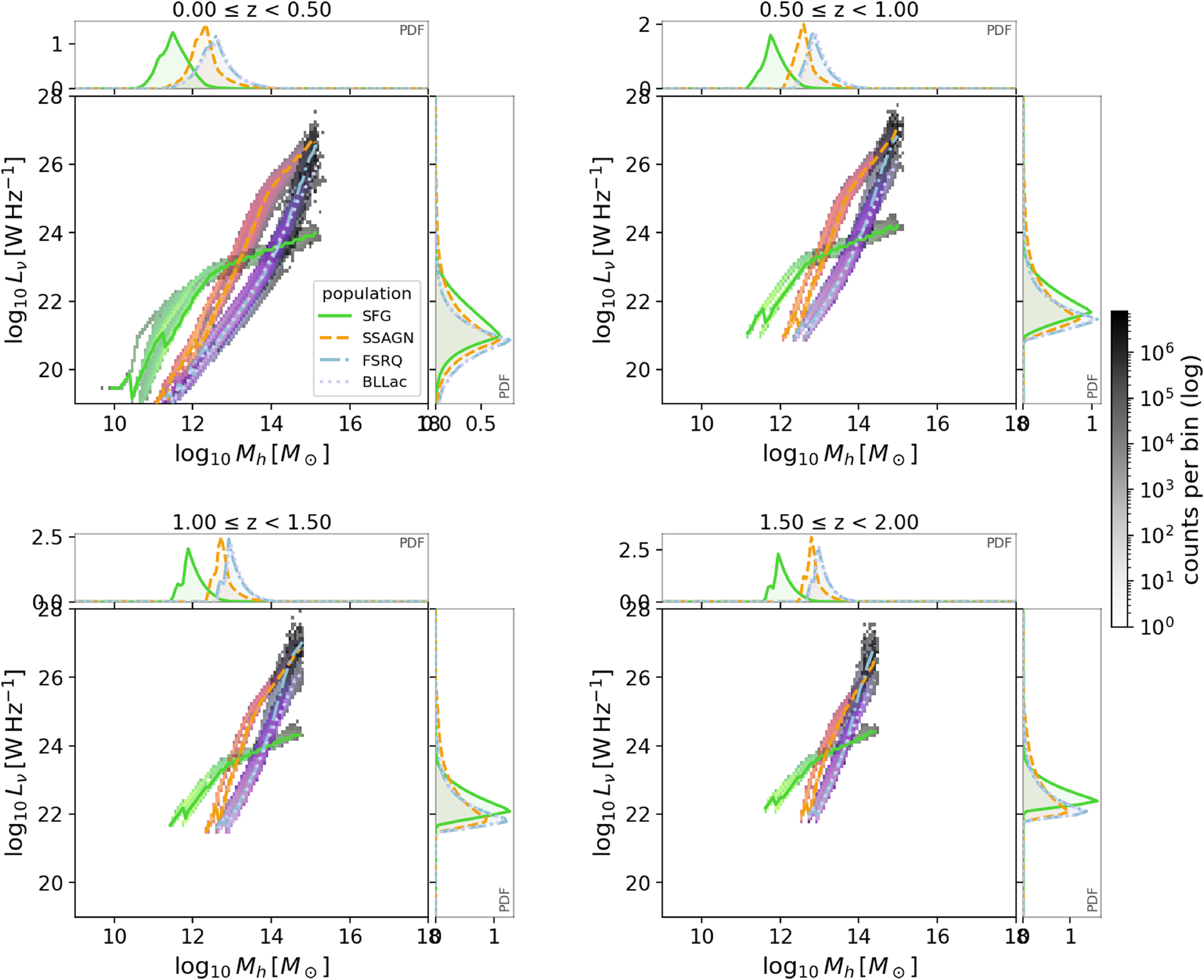
Figure 2 summarises the delivered mapping. SFGs occupy lower-mass halos and lower $L_\nu$
; steep-spectrum AGN extend to higher
$L_\nu$
; steep-spectrum AGN extend to higher $M_h$
with a steeper L–M trend; beamed subclasses (FSRQ, BLLac) preferentially inhabit the most massive halos and dominate the bright tail. With increasing redshift, median ridge-lines shift as expected from K-corrections and the evolving halo supply, and the per-population marginals narrow modestly.
$M_h$
with a steeper L–M trend; beamed subclasses (FSRQ, BLLac) preferentially inhabit the most massive halos and dominate the bright tail. With increasing redshift, median ridge-lines shift as expected from K-corrections and the evolving halo supply, and the per-population marginals narrow modestly.
All populations – radio luminosity vs. halo mass with per-population marginals (shared density scale). Each panel shows 2D binned abundances in a fixed redshift window; coloured semi-transparent maps overlay populations (SFG solid, SSAGN dashed, FSRQ dash-dot, BLLac dotted). All density layers share the same logarithmic colourbar, so intensity is directly comparable across populations and panels. Solid lines trace the median of $\log_{10}L_\nu$
at fixed
$\log_{10}L_\nu$
at fixed $\log_{10}M_h$
. The small top (right) axes show, for each population, the normalised marginal PDFs
$\log_{10}M_h$
. The small top (right) axes show, for each population, the normalised marginal PDFs $p(\log_{10}M_h)$
and
$p(\log_{10}M_h)$
and $p(\log_{10}L_\nu)$
– with
$p(\log_{10}L_\nu)$
– with $\int p\,{d}\log M_h=1$
and
$\int p\,{d}\log M_h=1$
and $\int p\,{d}\log L=1$
. SFG peak at lower host masses and luminosities; SSAGN extend to higher
$\int p\,{d}\log L=1$
. SFG peak at lower host masses and luminosities; SSAGN extend to higher $M_h$
with a steeper
$M_h$
with a steeper $L_\nu$
–
$L_\nu$
– $M_h$
trend; FSRQ and BL Lac preferentially inhabit the most massive halos and dominate the bright radio tail. With increasing redshift, the medians shift to higher
$M_h$
trend; FSRQ and BL Lac preferentially inhabit the most massive halos and dominate the bright radio tail. With increasing redshift, the medians shift to higher $M_h$
and the PDFs narrow, reflecting both selection effects and the evolving halo-occupation mix.
$M_h$
and the PDFs narrow, reflecting both selection effects and the evolving halo-occupation mix.
We track requested versus hosted counts per slice and population (Section 4.5). The hosted fraction is high across all panels; occasional *NH rows appear only at very low z and $L_\nu$
and are negligible for the selections used. In the RLF grids we show the model projected on the same (L, z) grid alongside the host-assigned estimate; the two agree within uncertainties over the full dynamic range.
$L_\nu$
and are negligible for the selections used. In the RLF grids we show the model projected on the same (L, z) grid alongside the host-assigned estimate; the two agree within uncertainties over the full dynamic range.
The host-assigned catalogue embeds a clear bias hierarchy – SFG $\lt$
SSAGN
$\lt$
SSAGN $\lt$
FSRQ/BL Lac – set by the actual halo field under the survey selection. Because our population-weighted apportionment keeps the hosted mixture close to the requested mixture for any flux/SNR cut, changes in
$\lt$
FSRQ/BL Lac – set by the actual halo field under the survey selection. Because our population-weighted apportionment keeps the hosted mixture close to the requested mixture for any flux/SNR cut, changes in $w(\theta)$
across selections reflect projection kernels rather than a reversal of intrinsic bias ordering. This alignment of mixture, bias hierarchy, and selection is exactly what multi-tracer
$w(\theta)$
across selections reflect projection kernels rather than a reversal of intrinsic bias ordering. This alignment of mixture, bias hierarchy, and selection is exactly what multi-tracer $f_\mathrm{NL}$
estimators require.
$f_\mathrm{NL}$
estimators require.
5.3. The angular correlation function
Our goal in this section is to verify that the catalogue places each population in environments consistent with their expected large-scale bias, and to produce clustering summaries that feed the PNG analysis in Paper 2. We therefore measure the two-point angular correlation of the simulated sky, both in configuration space, $w(\theta)$
, and in harmonic space,
$w(\theta)$
, and in harmonic space, $C_\ell$
. Given a redshift kernel
$C_\ell$
. Given a redshift kernel $\phi(z)$
(from the n(z) of each population), these observables probe the projection of the 3D matter power spectrum modulated by the tracers’ bias, so their amplitudes and slopes are sensitive to the typical host halo masses of SFGs versus AGN subclasses and how survey selections reshape
$\phi(z)$
(from the n(z) of each population), these observables probe the projection of the 3D matter power spectrum modulated by the tracers’ bias, so their amplitudes and slopes are sensitive to the typical host halo masses of SFGs versus AGN subclasses and how survey selections reshape $\phi(z)$
.
$\phi(z)$
.
Concretely, we compute $w(\theta)$
for AGN and SFG samples (and for specific survey-like cuts), fit a compact power-law model
$w(\theta)$
for AGN and SFG samples (and for specific survey-like cuts), fit a compact power-law model $w(\theta)=A(\theta/\theta_0)^{1-\gamma}$
over
$w(\theta)=A(\theta/\theta_0)^{1-\gamma}$
over $0.02^\circ$
–
$0.02^\circ$
– $1^\circ$
to quote comparable amplitudes and slopes, and cross-check in harmonic space by fitting
$1^\circ$
to quote comparable amplitudes and slopes, and cross-check in harmonic space by fitting $C_\ell$
with fixed
$C_\ell$
with fixed $\phi(z)$
templates to infer effective linear bias (both constant and gently evolving with redshift).
$\phi(z)$
templates to infer effective linear bias (both constant and gently evolving with redshift).
5.3.1. Definitions and modelling
We quantify angular clustering with the two-point correlation function $w(\theta)$
, related to the angular power spectrum
$w(\theta)$
, related to the angular power spectrum $C_\ell$
by
$C_\ell$
by
 \begin{equation}w(\theta)\;=\;\sum_{\ell=0}^{\infty}\frac{2\ell+1}{4\pi}\,C_\ell\,P_\ell(\cos\theta)\;\simeq\;\int\frac{\ell\,{d}\ell}{2\pi}\,J_0(\ell\theta)\,C_\ell,\end{equation}
where the Bessel form is accurate for small angles. In the Limber regime, the auto-spectrum for a population $X\in\{\mathrm{AGN},\mathrm{SFG}\}$
is
$X\in\{\mathrm{AGN},\mathrm{SFG}\}$
is
 \begin{align} C_\ell^{XX}&=\int {d}z\;\underbrace{\frac{H(z)}{\chi^2(z)}\,\phi_X^2(z)}_{\text{projection}}\;\underbrace{b_X^2(k,z)\,D^2(z)}_{\text{bias/growth}}\;\nonumber\\[3pt] &\quad \times P_m\!\left(k=\frac{\ell+1/2}{\chi(z)},z\right),\end{align}
with comoving distance $\chi(z)$
, Hubble rate H(z), linear growth D(z), matter spectrum
$\chi(z)$
, Hubble rate H(z), linear growth D(z), matter spectrum $P_m$
, and a normalised redshift kernel
$P_m$
, and a normalised redshift kernel $\phi_X(z)$
(unit area).
$\phi_X(z)$
(unit area).
Across a finite angular decade the observed slope of $w(\theta)$
reflects a weighted average of the 3D logarithmic slope
$w(\theta)$
reflects a weighted average of the 3D logarithmic slope $ {d}\ln[P_m\,b_X^2]/{d}\ln k $
evaluated at
$ {d}\ln[P_m\,b_X^2]/{d}\ln k $
evaluated at $k\simeq \ell/\chi(z)$
, convolved with
$k\simeq \ell/\chi(z)$
, convolved with $\phi_X^2$
. For direct comparison to the literature and to quote compact summary numbers we fit a power law
$\phi_X^2$
. For direct comparison to the literature and to quote compact summary numbers we fit a power law
 \begin{equation}w(\theta)=A\left(\frac{\theta}{\theta_0}\right)^{1-\gamma},\end{equation}
using full covariances where available and a pivot $\theta_0$
taken to be the geometric mean of the fitted
$\theta_0$
taken to be the geometric mean of the fitted $\theta$
to minimise the A–
$\theta$
to minimise the A– $\gamma$
covariance. Unless stated otherwise we fit over
$\gamma$
covariance. Unless stated otherwise we fit over $\theta\in[0.02^\circ,\,1.0^\circ]$
(
$\theta\in[0.02^\circ,\,1.0^\circ]$
( $\ell\simeq 50$
–400).
$\ell\simeq 50$
–400).
To interpret slope changes induced by selections, we also quote effective redshifts and distances computed with Limber-like weights
 \begin{align} W_X(z)\;&\propto\;\frac{H(z)}{\chi^2(z)}\,\phi_X^2(z)\,D^2(z),\qquad \\[-10pt] \nonumber \end{align}
 \begin{align} z_{\mathrm{eff}, X}&=\frac{\int \! W_X(z)\,z\,{d}z}{\int \! W_X(z)\,{d}z},\qquad \\[-10pt] \nonumber \end{align}
 \begin{align} \chi_{\mathrm{eff}, X}&=\frac{\int \! W_X(z)\,\chi(z)\,{d}z}{\int \! W_X(z)\,{d}z}. \\[10pt] \nonumber \end{align}
A fixed angular separation then corresponds to a characteristic projected comoving scale
 \begin{equation}r_\perp(\theta)=\theta\,\chi_{\mathrm{eff}, X}.\end{equation}
5.3.2. Raw GHOST sample
In Figure 3, we present the angular correlation function of the full GHOST sample showing AGN lying above SFG in amplitude across all $\theta$
, consistent with their higher bias and host-halo masses. Power-law fits give
$\theta$
, consistent with their higher bias and host-halo masses. Power-law fits give $\gamma_\mathrm{AGN}=1.886\pm0.028$
and
$\gamma_\mathrm{AGN}=1.886\pm0.028$
and $\gamma_\mathrm{{SFG}}=1.647\pm0.076$
. The effective depths are
$\gamma_\mathrm{{SFG}}=1.647\pm0.076$
. The effective depths are $(z_\mathrm{eff},\chi_\mathrm{eff})=(0.318,\,1.22 \mathrm{Gpc})$
for AGN and
$(z_\mathrm{eff},\chi_\mathrm{eff})=(0.318,\,1.22 \mathrm{Gpc})$
for AGN and $(0.602,\,2.12\,\mathrm{Gpc})$
for SFG, so
$(0.602,\,2.12\,\mathrm{Gpc})$
for SFG, so $r_\perp(0.05^\circ)=(1.06,\,1.85) \mathrm{Mpc}$
, respectively. The shallower SFG slope in the raw GHOST sample is naturally explained by their broader, higher-z kernel
$r_\perp(0.05^\circ)=(1.06,\,1.85) \mathrm{Mpc}$
, respectively. The shallower SFG slope in the raw GHOST sample is naturally explained by their broader, higher-z kernel $\phi(z)$
, which mixes a wider range of
$\phi(z)$
, which mixes a wider range of $k=\ell/\chi$
in projection (Equations 20–24).
$k=\ell/\chi$
in projection (Equations 20–24).
Raw GHOST sample: Angular correlation function $w(\theta)$
for AGN (blue triangles) and SFG (orange circles). Solid lines show inverse-variance weighted power-law fits
$w(\theta)$
for AGN (blue triangles) and SFG (orange circles). Solid lines show inverse-variance weighted power-law fits $w(\theta)=A(\theta/\theta_0)^{1-\gamma}$
over
$w(\theta)=A(\theta/\theta_0)^{1-\gamma}$
over $\theta\in[0.02^\circ,\,1.0^\circ]$
; shaded bands are the propagated
$\theta\in[0.02^\circ,\,1.0^\circ]$
; shaded bands are the propagated $1\sigma$
model uncertainties from the
$1\sigma$
model uncertainties from the $(A,\gamma)$
covariance. Best-fit slopes are
$(A,\gamma)$
covariance. Best-fit slopes are $\gamma_\mathrm{AGN}=1.886\pm0.028$
and
$\gamma_\mathrm{AGN}=1.886\pm0.028$
and $\gamma_\mathrm{{SFG}}=1.647\pm0.076$
. The lower panel shows data
$\gamma_\mathrm{{SFG}}=1.647\pm0.076$
. The lower panel shows data $-$
fit residuals. The amplitude ordering AGN
$-$
fit residuals. The amplitude ordering AGN $\gt$
SFG reflects the intrinsic bias hierarchy, while the slightly shallower SFG slope is consistent with a broader, higher-z kernel
$\gt$
SFG reflects the intrinsic bias hierarchy, while the slightly shallower SFG slope is consistent with a broader, higher-z kernel $\phi(z)$
that mixes more
$\phi(z)$
that mixes more $k=\ell/\chi(z)$
in projection (Equations 19 and 20).
$k=\ell/\chi(z)$
in projection (Equations 19 and 20).

5.3.3. VLA–COSMOS 1.4 GHz
Applying the $L_{1.4}\gtrless L_\mathrm{cross}(z)$
selection, as detailed in Section 5.1.2, compresses the SFG kernel to very low z. We find
$L_{1.4}\gtrless L_\mathrm{cross}(z)$
selection, as detailed in Section 5.1.2, compresses the SFG kernel to very low z. We find $\gamma_\mathrm{AGN}=1.858\pm0.041$
and
$\gamma_\mathrm{AGN}=1.858\pm0.041$
and $\gamma_\mathrm{{SFG}}=1.667\pm0.010$
, with
$\gamma_\mathrm{{SFG}}=1.667\pm0.010$
, with $(z_\mathrm{eff},\chi_\mathrm{eff})=(0.339,\,1.30\,\mathrm{Gpc})$
for AGN and
$(z_\mathrm{eff},\chi_\mathrm{eff})=(0.339,\,1.30\,\mathrm{Gpc})$
for AGN and $(0.094,\,0.41\,\mathrm{Gpc})$
for SFG, implying
$(0.094,\,0.41\,\mathrm{Gpc})$
for SFG, implying $r_\perp(0.05^\circ)=(1.14,\,0.35)\,\mathrm{Mpc}$
. In Figure 4, the SFG correlation lies above the AGN over the fitted range. This does not imply a larger intrinsic SFG bias; it follows from the projection weights in the Limber integral, which scale as
$r_\perp(0.05^\circ)=(1.14,\,0.35)\,\mathrm{Mpc}$
. In Figure 4, the SFG correlation lies above the AGN over the fitted range. This does not imply a larger intrinsic SFG bias; it follows from the projection weights in the Limber integral, which scale as $\phi^2(z)/\chi^2(z)$
. Our selection compresses the SFG kernel to very low redshift (
$\phi^2(z)/\chi^2(z)$
. Our selection compresses the SFG kernel to very low redshift ( $z_\mathrm{eff}\simeq0.094$
,
$z_\mathrm{eff}\simeq0.094$
, $\chi_\mathrm{eff}\simeq0.41\,\mathrm{Gpc}$
) while the AGN kernel sits higher (
$\chi_\mathrm{eff}\simeq0.41\,\mathrm{Gpc}$
) while the AGN kernel sits higher ( $z_\mathrm{eff}\simeq0.339$
,
$z_\mathrm{eff}\simeq0.339$
, $\chi_\mathrm{eff}\simeq1.30\,\mathrm{Gpc}$
). The resulting geometric factor
$\chi_\mathrm{eff}\simeq1.30\,\mathrm{Gpc}$
). The resulting geometric factor $(\chi_\mathrm{AGN}/\chi_\mathrm{{SFG}})^2\simeq(1.30/0.41)^2\!\approx\!10$
boosts the projected SFG amplitude and can outweigh the larger AGN bias, thereby producing the observed inversion in
$(\chi_\mathrm{AGN}/\chi_\mathrm{{SFG}})^2\simeq(1.30/0.41)^2\!\approx\!10$
boosts the projected SFG amplitude and can outweigh the larger AGN bias, thereby producing the observed inversion in $w(\theta)$
. The residual shape mismatch – most evident in the flatter SFG slope – likely reflects blending of one- and two-halo terms when projecting such a low-z kernel over
$w(\theta)$
. The residual shape mismatch – most evident in the flatter SFG slope – likely reflects blending of one- and two-halo terms when projecting such a low-z kernel over $0.02^\circ\!-\!1^\circ$
(
$0.02^\circ\!-\!1^\circ$
( $r_\perp\!\sim\!0.14\!-\!7\,\mathrm{Mpc}$
), and modelling choices that suppress small-scale power (e.g. our current radio-SFG occupation lacks an explicit satellite component). These effects account for the difference in gradient while preserving the relative bias hierarchy that underpins the multi-tracer analysis.
$r_\perp\!\sim\!0.14\!-\!7\,\mathrm{Mpc}$
), and modelling choices that suppress small-scale power (e.g. our current radio-SFG occupation lacks an explicit satellite component). These effects account for the difference in gradient while preserving the relative bias hierarchy that underpins the multi-tracer analysis.
VLA-COSMOS selection (1.4 GHz): $w(\theta)$
for AGN and SFG after the
$w(\theta)$
for AGN and SFG after the $L_{1.4}\gtrless L_\mathrm{cross}(z)$
selection function detailed in Section 5.1.2. Solid curves are our power-law fits over
$L_{1.4}\gtrless L_\mathrm{cross}(z)$
selection function detailed in Section 5.1.2. Solid curves are our power-law fits over $\theta\in[0.02^\circ,\,1.0^\circ]$
(shaded
$\theta\in[0.02^\circ,\,1.0^\circ]$
(shaded $1\sigma$
bands); dotted lines and translucent bands show the literature reference for AGN and SFG, respectively. We obtain
$1\sigma$
bands); dotted lines and translucent bands show the literature reference for AGN and SFG, respectively. We obtain $\gamma_\mathrm{AGN}=1.858\pm0.041$
and
$\gamma_\mathrm{AGN}=1.858\pm0.041$
and $\gamma_\mathrm{{SFG}}=1.667\pm0.010$
. The SFG amplitude lies above the reference at large scales and the slope is slightly flatter. From the effective-depth summary (Table 3) the SFG kernel compresses to
$\gamma_\mathrm{{SFG}}=1.667\pm0.010$
. The SFG amplitude lies above the reference at large scales and the slope is slightly flatter. From the effective-depth summary (Table 3) the SFG kernel compresses to $z_\mathrm{eff}\simeq0.094$
and
$z_\mathrm{eff}\simeq0.094$
and $\chi_\mathrm{eff}\simeq0.41$
Gpc, so a fixed
$\chi_\mathrm{eff}\simeq0.41$
Gpc, so a fixed $\theta$
probes small
$\theta$
probes small $r_\perp$
(e.g.
$r_\perp$
(e.g. $r_\perp(0.05^\circ)\approx0.35$
Mpc), flattening the angular scaling (Equations 24 and 25).
$r_\perp(0.05^\circ)\approx0.35$
Mpc), flattening the angular scaling (Equations 24 and 25).

5.3.4. VLA–COSMOS 3 GHz
The same pattern repeats at 3 GHz, with the selection described in Section 5.1.3: $\gamma_\mathrm{AGN}=1.903\pm0.037$
and
$\gamma_\mathrm{AGN}=1.903\pm0.037$
and $\gamma_\mathrm{{SFG}}=1.662\pm0.010$
, with
$\gamma_\mathrm{{SFG}}=1.662\pm0.010$
, with $(z_\mathrm{eff},\chi_\mathrm{eff})=(0.313,\,1.21\,\mathrm{Gpc})$
for AGN and
$(z_\mathrm{eff},\chi_\mathrm{eff})=(0.313,\,1.21\,\mathrm{Gpc})$
for AGN and $(0.161,\,0.67\,\mathrm{Gpc})$
for SFG, hence
$(0.161,\,0.67\,\mathrm{Gpc})$
for SFG, hence $r_\perp(0.05^\circ)=(1.05,\,0.59)\,\mathrm{Mpc}$
. Relative to the Hale et al. 3 GHz bands our SFG points lie higher and show a slightly shallower slope, eventually overtaking the AGN at large angles. This behaviour is expected from the different redshift kernels: the SFG selection sits at lower
$r_\perp(0.05^\circ)=(1.05,\,0.59)\,\mathrm{Mpc}$
. Relative to the Hale et al. 3 GHz bands our SFG points lie higher and show a slightly shallower slope, eventually overtaking the AGN at large angles. This behaviour is expected from the different redshift kernels: the SFG selection sits at lower $\chi_\mathrm{ eff}$
, so the projection integral schematically
$\chi_\mathrm{ eff}$
, so the projection integral schematically $w(\theta)\!\propto\!\int dz\,\phi^2(z)\,b^2(z)\,D^2(z)/\chi^2(z)$
weights it more strongly, and the same angular range probes smaller
$w(\theta)\!\propto\!\int dz\,\phi^2(z)\,b^2(z)\,D^2(z)/\chi^2(z)$
weights it more strongly, and the same angular range probes smaller $r_\perp$
, mixing some one-halo power into the fitted scales and flattening the apparent slope. By contrast, the AGN kernel projects to larger
$r_\perp$
, mixing some one-halo power into the fitted scales and flattening the apparent slope. By contrast, the AGN kernel projects to larger $r_\perp$
where the two-halo term dominates and the slope is steeper. Residual differences with the Hale et al. (Reference Hale, Jarvis, Delvecchio, Hatfield and Novak2018) bands are therefore plausibly explained by modest kernel mismatches (e.g. a slight SFG overweight at
$r_\perp$
where the two-halo term dominates and the slope is steeper. Residual differences with the Hale et al. (Reference Hale, Jarvis, Delvecchio, Hatfield and Novak2018) bands are therefore plausibly explained by modest kernel mismatches (e.g. a slight SFG overweight at $z\!\lesssim\!0.3$
in the mocks), survey-specific treatments of integral-constraint and close pairs/multi-component sources that suppress small-angle power, and minor AGN/SFG cross-contamination near the luminosity split. The cross-frequency consistency (compare 1.4 GHz) supports the interpretation that these are selection-driven projection effects rather than frequency-dependent systematics. The ACF is shown in Figure 5.
$z\!\lesssim\!0.3$
in the mocks), survey-specific treatments of integral-constraint and close pairs/multi-component sources that suppress small-angle power, and minor AGN/SFG cross-contamination near the luminosity split. The cross-frequency consistency (compare 1.4 GHz) supports the interpretation that these are selection-driven projection effects rather than frequency-dependent systematics. The ACF is shown in Figure 5.
5.3.5. Picture across frequencies
The differences we see across the raw, Magliocchetti and Hale-like samples are driven primarily by how each selection reshapes the redshift kernel $\phi(z)$
, not by any change in the intrinsic bias ordering. In Equation (20) the amplitude scales as
$\phi(z)$
, not by any change in the intrinsic bias ordering. In Equation (20) the amplitude scales as $b^2\,\phi^2/\chi^2$
and the slope reflects which 3D wavenumbers are projected (
$b^2\,\phi^2/\chi^2$
and the slope reflects which 3D wavenumbers are projected ( $k\simeq \ell/\chi$
) given the kernel. Cuts that compress the SFG kernel to lower redshift (e.g. luminosity splits or high S/N survey selection functions) increase
$k\simeq \ell/\chi$
) given the kernel. Cuts that compress the SFG kernel to lower redshift (e.g. luminosity splits or high S/N survey selection functions) increase $\phi^2/\chi^2$
and shift the map towards larger k, yielding the observed ‘lift and flattening’ of SFG
$\phi^2/\chi^2$
and shift the map towards larger k, yielding the observed ‘lift and flattening’ of SFG $w(\theta)$
. AGN kernels move much less under the same cuts, so the intrinsic hierarchy
$w(\theta)$
. AGN kernels move much less under the same cuts, so the intrinsic hierarchy $b_\mathrm{AGN} \gt b_\mathrm{{SFG}}$
remains intact.
$b_\mathrm{AGN} \gt b_\mathrm{{SFG}}$
remains intact.
This explains the apparent discrepancy between the Magliocchetti and Hale measurements: once their selection functions are emulated, both behaviours arise naturally from projection effects with a fixed bias ordering. The cross-frequency consistency (1.4 vs 3 GHz) further shows the effect is selection-driven rather than band-dependent. For multi-tracer $f_\mathrm{NL}$
applications, the lesson is operational: clustering inferences must be made with tracer-specific
$f_\mathrm{NL}$
applications, the lesson is operational: clustering inferences must be made with tracer-specific $\phi(z)$
that match the actual survey survey selection functions; otherwise slope and amplitude shifts can be misread as bias changes. Here we carry forward bias parameters together with the matched kernels to ensure the large-scale modes relevant for
$\phi(z)$
that match the actual survey survey selection functions; otherwise slope and amplitude shifts can be misread as bias changes. Here we carry forward bias parameters together with the matched kernels to ensure the large-scale modes relevant for $f_\mathrm{NL}$
are interpreted consistently. The statistics of the ACF are summarised in Table 3.
$f_\mathrm{NL}$
are interpreted consistently. The statistics of the ACF are summarised in Table 3.
Projection summary for AGN and SFG by selection. Errors are $1\sigma$
from power-law fits over
$1\sigma$
from power-law fits over $\theta\in[0.02^\circ,0.5^\circ]$
. Effective depths use the Limber-like weights of Equation (24). We quote the characteristic projected comoving separation
$\theta\in[0.02^\circ,0.5^\circ]$
. Effective depths use the Limber-like weights of Equation (24). We quote the characteristic projected comoving separation $r_\perp(\theta)=\theta\,\chi_\mathrm{eff}$
at three angles.
$r_\perp(\theta)=\theta\,\chi_\mathrm{eff}$
at three angles.
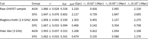
Bias fits from $C_\ell$
over
$C_\ell$
over $\ell\in[40\,,\,250]$
. We fit a constant-bias model (
$\ell\in[40\,,\,250]$
. We fit a constant-bias model ( $b=$
const) and an evolving form
$b=$
const) and an evolving form $b(z)=b_0(1+z)^\zeta$
. Quoted
$b(z)=b_0(1+z)^\zeta$
. Quoted $\chi^2$
values are for the best fit of each model. The last column gives the constant-bias ratio
$\chi^2$
values are for the best fit of each model. The last column gives the constant-bias ratio $b/b_\mathrm{{SFG}}$
.
$b/b_\mathrm{{SFG}}$
.

5.4. Angular power spectra and bias fits
We model the auto-spectra of each radio population $X\in\{\mathrm{SFG},\mathrm{SSAGN},\mathrm{BLLac},\mathrm{FSRQ}\}$
in the Limber regime using Equation (20). We construct, for each tracer, a template
$X\in\{\mathrm{SFG},\mathrm{SSAGN},\mathrm{BLLac},\mathrm{FSRQ}\}$
in the Limber regime using Equation (20). We construct, for each tracer, a template $T_\ell^X$
by evaluating Equation (20) with a unit, redshift-independent bias (i.e.
$T_\ell^X$
by evaluating Equation (20) with a unit, redshift-independent bias (i.e. $b(z) \equiv 1$
). The measured spectrum in a given
$b(z) \equiv 1$
). The measured spectrum in a given $\ell$
-band then determines an overall amplitude related to the bias.
$\ell$
-band then determines an overall amplitude related to the bias.
We fit two bias models over $\ell\in[\ell_{\min},\ell_{\max}]$
(default 40–250), after sanitising n(z) (Section 5.6) and optionally subtracting a shot component from the auto-correlations when available.
$\ell\in[\ell_{\min},\ell_{\max}]$
(default 40–250), after sanitising n(z) (Section 5.6) and optionally subtracting a shot component from the auto-correlations when available.
5.4.1. Constant bias
We assume $b_X(z) = b_X$
and fit an amplitude
$b_X(z) = b_X$
and fit an amplitude $a_X = b_X^2$
against the fixed template
$a_X = b_X^2$
against the fixed template $T_\ell^X$
. Using (optionally) Knox weights
$T_\ell^X$
. Using (optionally) Knox weights $w_\ell=[2/((2\ell+1)f_\mathrm{sky})]/\sigma^2_\ell$
or per-band errors we solve the weighted least-squares problem
$w_\ell=[2/((2\ell+1)f_\mathrm{sky})]/\sigma^2_\ell$
or per-band errors we solve the weighted least-squares problem
 \begin{equation}\widehat{a}_X \;=\; \frac{\sum_\ell w_\ell\,T_\ell^X\,C_\ell^{\mathrm{obs}}}{\sum_\ell w_\ell\,(T_\ell^X)^2},\qquad\widehat{b}_X\;=\;\sqrt{\widehat{a}_X}\,,\end{equation}
with error propagation $\sigma^2_{a}\simeq 1/\!\sum_\ell w_\ell(T_\ell^X)^2$
and
$\sigma^2_{a}\simeq 1/\!\sum_\ell w_\ell(T_\ell^X)^2$
and $\sigma_b\simeq \sigma_a/(2\,\widehat{b})$
. Goodness of fit is summarised by
$\sigma_b\simeq \sigma_a/(2\,\widehat{b})$
. Goodness of fit is summarised by $\chi^2=\sum_\ell w_\ell(C_\ell^\mathrm{obs}-\widehat{a}\,T_\ell)^2$
.
$\chi^2=\sum_\ell w_\ell(C_\ell^\mathrm{obs}-\widehat{a}\,T_\ell)^2$
.
VLA-COSMOS selection (3 GHz): Same as Figure 4 but for the 3 GHz cut (Section 5.1.3. Our fits give $\gamma_\mathrm{AGN}=1.903\pm0.037$
and
$\gamma_\mathrm{AGN}=1.903\pm0.037$
and $\gamma_\mathrm{{SFG}}=1.662\pm0.010$
. AGN closely follow the band from Hale et al. (Reference Hale, Jarvis, Delvecchio, Hatfield and Novak2018), while SFG sit high and slightly flatter. The projection summary (Table 3) shows
$\gamma_\mathrm{{SFG}}=1.662\pm0.010$
. AGN closely follow the band from Hale et al. (Reference Hale, Jarvis, Delvecchio, Hatfield and Novak2018), while SFG sit high and slightly flatter. The projection summary (Table 3) shows $z_\mathrm{eff,\,SFG}\simeq0.161$
and
$z_\mathrm{eff,\,SFG}\simeq0.161$
and $\chi_\mathrm{eff,\,SFG}\simeq0.67$
Gpc (so
$\chi_\mathrm{eff,\,SFG}\simeq0.67$
Gpc (so $r_\perp(0.05^\circ)\approx0.59$
Mpc), again explaining the slope change as a selection-driven projection effect rather than frequency-dependent systematics. Residuals (lower panel) are shown relative to the fitted power laws.
$r_\perp(0.05^\circ)\approx0.59$
Mpc), again explaining the slope change as a selection-driven projection effect rather than frequency-dependent systematics. Residuals (lower panel) are shown relative to the fitted power laws.
 $C_\ell$
bias fits by population. Points show measured bandpowers; dashed lines are best-fit constant-bias models (
$C_\ell$
bias fits by population. Points show measured bandpowers; dashed lines are best-fit constant-bias models ( $b=$
const) and solid lines are evolving models
$b=$
const) and solid lines are evolving models $b(z)=b_0(1+z)^\zeta$
, both fit over
$b(z)=b_0(1+z)^\zeta$
, both fit over $\ell\in[40,250]$
. Numerical values are listed in Table 4. The amplitude ordering SFG
$\ell\in[40,250]$
. Numerical values are listed in Table 4. The amplitude ordering SFG $\lt$
SSAGN
$\lt$
SSAGN $\lesssim$
FSRQ
$\lesssim$
FSRQ $\simeq$
BLLac and the positive
$\simeq$
BLLac and the positive $\zeta$
for AGN are consistent with the halo–mass distributions and the configuration-space results (Section 5.3).
$\zeta$
for AGN are consistent with the halo–mass distributions and the configuration-space results (Section 5.3).

Figure 6. Long description
Panel A: A line graph titled SFG. The x-axis is labeled with the variable l and ranges from 40 to 200. The y-axis is labeled G1 and ranges from 0 to 10^-6. The graph includes two lines: a dashed orange line representing a constant-bias model with const b=1.55 and a solid green line representing an evolving model with evol b0=1.87, alpha=1.09. Data points are marked with blue symbols. Panel B: A line graph titled SSAGN. The x-axis is labeled with the variable l and ranges from 40 to 200. The y-axis is labeled G1 and ranges from 0 to 10^-6. The graph includes two lines: a dashed orange line representing a constant-bias model with const b=1.95 and a solid green line representing an evolving model with evol b0=3.05, alpha=3.41. Data points are marked with blue symbols. Panel C: A line graph titled BLLac. The x-axis is labeled with the variable l and ranges from 40 to 200. The y-axis is labeled G1 and ranges from 0 to 10^-6. The graph includes two lines: a dashed orange line representing a constant-bias model with const b=2.32 and a solid green line representing an evolving model with evol b0=4.35, alpha=4.19. Data points are marked with blue symbols. Panel D: A line graph titled FSRQ. The x-axis is labeled with the variable l and ranges from 40 to 200. The y-axis is labeled G1 and ranges from 0 to 10^-6. The graph includes two lines: a dashed orange line representing a constant-bias model with const b=2.27 and a solid green line representing an evolving model with evol b0=4.64, alpha=4.71. Data points are marked with blue symbols.
5.4.2. Evolving bias
We test a minimal two-parameter form
 \begin{equation}b_X(z)=b_{0,X}\,(1+z)^{\zeta_X}.\end{equation}
Within our pipeline this redshift dependence is folded into the shape of the projection kernel by replacing $\phi_X(z)\!\to\!\phi_X(z)\,{(1+z)^{\zeta_X}}$
(and re-normalising to unit area), while keeping the overall amplitude as
$\phi_X(z)\!\to\!\phi_X(z)\,{(1+z)^{\zeta_X}}$
(and re-normalising to unit area), while keeping the overall amplitude as $b_0^2$
. For each tracer we form the profile likelihood in
$b_0^2$
. For each tracer we form the profile likelihood in $\zeta$
by optimising
$\zeta$
by optimising $b_0$
at fixed
$b_0$
at fixed $\zeta$
using Equation (26), that is,
$\zeta$
using Equation (26), that is, $\widehat b_0(\zeta)=\arg\min_{b_0}\chi^2(b_0,\zeta)$
. We then select
$\widehat b_0(\zeta)=\arg\min_{b_0}\chi^2(b_0,\zeta)$
. We then select $(\widehat b_0(\widehat\zeta),\widehat\zeta)$
with
$(\widehat b_0(\widehat\zeta),\widehat\zeta)$
with $\widehat\zeta=\arg\min_\zeta \chi^2(\widehat b_0(\zeta),\zeta)$
.
$\widehat\zeta=\arg\min_\zeta \chi^2(\widehat b_0(\zeta),\zeta)$
.
5.4.3. Results
Table 4 summarises the fits. In the constant model we find the expected hierarchy $b_\mathrm{SFG} \lt b_\mathrm{SSAGN}\lesssim b_\mathrm{FSRQ}\simeq b_\mathrm{BLLac}$
. The evolving model always yields a slightly lower
$b_\mathrm{SFG} \lt b_\mathrm{SSAGN}\lesssim b_\mathrm{FSRQ}\simeq b_\mathrm{BLLac}$
. The evolving model always yields a slightly lower $\chi^2$
statistic, indicating better fit, with
$\chi^2$
statistic, indicating better fit, with $(\zeta,\ b_0)$
increasing from SFG to radio-loud AGN, consistent with rarer, more strongly biased hosts at higher redshift. Figure 6 shows the measured bandpowers with the best-fit constant (dashed) and evolving (solid) curves.
$(\zeta,\ b_0)$
increasing from SFG to radio-loud AGN, consistent with rarer, more strongly biased hosts at higher redshift. Figure 6 shows the measured bandpowers with the best-fit constant (dashed) and evolving (solid) curves.
5.4.4. Implications
The bias ordering mirrors the halo–mass distributions inferred from the catalogue: SFG peak at lower masses ( $\sim$ $10^{12}$
M
$10^{12}$
M $_\odot$
) while AGN subclasses peak at higher masses (few
$_\odot$
) while AGN subclasses peak at higher masses (few $\times 10^{12.5-13}$
M
$\times 10^{12.5-13}$
M $_\odot$
), naturally producing larger large-scale clustering amplitudes. The mild preference for positive
$_\odot$
), naturally producing larger large-scale clustering amplitudes. The mild preference for positive $\zeta$
in AGN (
$\zeta$
in AGN ( $\zeta\sim3$
–5) indicates bias growth with redshift, aligning with the picture of AGN inhabiting rarer halos at earlier times. Overall, the
$\zeta\sim3$
–5) indicates bias growth with redshift, aligning with the picture of AGN inhabiting rarer halos at earlier times. Overall, the $C_\ell$
fits and the configuration-space results (Section 5.3) are mutually consistent: amplitudes trace
$C_\ell$
fits and the configuration-space results (Section 5.3) are mutually consistent: amplitudes trace $b^2$
while the
$b^2$
while the $w(\theta)$
slope variations are explained by projection effects rather than changes in the underlying bias hierarchy.
$w(\theta)$
slope variations are explained by projection effects rather than changes in the underlying bias hierarchy.
Host halo mass PDFs by population. normalised distributions of $\log_{10}(M_h/M_\odot)$
(per dex) for SFG, SSAGN, BLLac, and FSRQ. Distributions for the AGN subclasses peak near
$\log_{10}(M_h/M_\odot)$
(per dex) for SFG, SSAGN, BLLac, and FSRQ. Distributions for the AGN subclasses peak near $10^{12.8-13}$
M
$10^{12.8-13}$
M $_\odot$
, while SFG peak near
$_\odot$
, while SFG peak near $10^{12}$
M
$10^{12}$
M $_\odot$
. The mass ordering maps onto the bias hierarchy measured in Section 5.4.
$_\odot$
. The mass ordering maps onto the bias hierarchy measured in Section 5.4.

5.5. Host halo mass distributions
To connect clustering amplitudes with halo occupation, we examine the distribution of host halo masses $M_h$
for each population. Figure 7 shows per-population PDFs of
$M_h$
for each population. Figure 7 shows per-population PDFs of $\log_{10}(M_h/M_\odot)$
(normalised per dex). Table 5 lists the median, the central 68% interval, and the sample size.
$\log_{10}(M_h/M_\odot)$
(normalised per dex). Table 5 lists the median, the central 68% interval, and the sample size.
The ordering is clear: SFG inhabit lower-mass halos (median $\log_{10}M_h \simeq 11.97$
), while all AGN subclasses peak near
$\log_{10}M_h \simeq 11.97$
), while all AGN subclasses peak near $\sim$ $10^{12.6-13.0}$
M
$10^{12.6-13.0}$
M $_\odot$
(SSAGN
$_\odot$
(SSAGN $\simeq12.65$
, BLLac
$\simeq12.65$
, BLLac $\simeq12.95$
, FSRQ
$\simeq12.95$
, FSRQ $\simeq12.92$
). The interquartile widths (IQR) are similar (
$\simeq12.92$
). The interquartile widths (IQR) are similar ( $\sim$
0.63–0.68 dex), indicating that the dominant difference is a shift in typical mass rather than a change in spread.
$\sim$
0.63–0.68 dex), indicating that the dominant difference is a shift in typical mass rather than a change in spread.
Because the large-scale bias b(M, z) is a monotonic function of halo mass (e.g. in peak-background split models),
 \begin{align}\begin{split}b(M,z)\; &=\;1+\frac{a\nu^2-1}{\delta_c}+\frac{2p}{\delta_c\,[1+(a\nu^2)^p]}\,,\qquad\\[2pt]\nu &\equiv \frac{\delta_c}{\sigma(M,z)} ,\end{split}\end{align}
(with $\delta_c\simeq1.686$
and
$\delta_c\simeq1.686$
and $(a,p)\approx(0.707,0.3)$
as a common choice), the
$(a,p)\approx(0.707,0.3)$
as a common choice), the $\sim$
0.7–1.0 dex upward shift from SFG to radio-loud AGN naturally implies larger b at the redshifts that dominate our projection. This is precisely what we measure from
$\sim$
0.7–1.0 dex upward shift from SFG to radio-loud AGN naturally implies larger b at the redshifts that dominate our projection. This is precisely what we measure from $C_\ell$
in Section 5.4: the constant-bias fits obey
$C_\ell$
in Section 5.4: the constant-bias fits obey $b_\mathrm{{SFG}} \lt b_\mathrm{{SSAGN}} \lesssim b_\mathrm{{FSRQ}} \simeq b_\mathrm{BLLac}$
, and the evolving model prefers positive
$b_\mathrm{{SFG}} \lt b_\mathrm{{SSAGN}} \lesssim b_\mathrm{{FSRQ}} \simeq b_\mathrm{BLLac}$
, and the evolving model prefers positive $\zeta$
for AGN, consistent with rarer halos at earlier times.
$\zeta$
for AGN, consistent with rarer halos at earlier times.
Summary of host halo mass distributions per population. We report the sample size N, the median $\mathrm{med}[\log_{10}M_h/M_\odot]$
, the central 68% interval (16th–84th percentiles), the IQR width, and the median offset relative to SFG.
$\mathrm{med}[\log_{10}M_h/M_\odot]$
, the central 68% interval (16th–84th percentiles), the IQR width, and the median offset relative to SFG.

Overall, the mass PDFs corroborate the bias/clustering hierarchy found in both configuration and harmonic space: AGN populate more massive halos than SFG, hence exhibit higher large-scale clustering amplitudes, while the small changes in $w(\theta)$
slope across selections are driven by projection (Section 5.3) rather than a reversal of the intrinsic bias-mass ordering.
$w(\theta)$
slope across selections are driven by projection (Section 5.3) rather than a reversal of the intrinsic bias-mass ordering.
5.6. Redshift distributions n(z)
Figure 8 shows normalised redshift distributions for the full GHOST catalogue and for AGN and SFG sub-samples (area under each curve equals unity). Before any survey selection, the total population peaks near $z\!\sim\!0.8$
with a long tail to
$z\!\sim\!0.8$
with a long tail to $z\gt3$
(median
$z\gt3$
(median $z=1.21$
, IQR
$z=1.21$
, IQR $0.74$
-
$0.74$
- $1.81$
). The AGN distribution is narrower (median
$1.81$
). The AGN distribution is narrower (median $z=0.85$
, IQR
$z=0.85$
, IQR $0.50$
–
$0.50$
– $1.31$
), while SFG peak at slightly higher redshift (median
$1.31$
), while SFG peak at slightly higher redshift (median $z=1.23$
, IQR
$z=1.23$
, IQR $0.75$
–
$0.75$
– $1.83$
) and maintain the broader high-z tail. This is consistent with radio-loud AGN dominating the bright counts at low z and SFG contributing increasingly towards the sub-mJy regime.
$1.83$
) and maintain the broader high-z tail. This is consistent with radio-loud AGN dominating the bright counts at low z and SFG contributing increasingly towards the sub-mJy regime.
At our pre-selection stage with the raw GHOST catalogue, the n(z) for SFG and AGN look consistent with the behaviour from deep $\unicode{x03BC}$
Jy radio surveys: SFG dominate at faint fluxes and exhibit a broad distribution that extends to
$\unicode{x03BC}$
Jy radio surveys: SFG dominate at faint fluxes and exhibit a broad distribution that extends to $z\approx4$
, while AGN show a more concentrated, lower z peak. Similar behaviour is seen in the acsLoTSS Deep fields (Best et al. Reference Best2023; Bonzini et al. Reference Bonzini, Padovani, Mainieri, Kellermann, Miller, Rosati, Tozzi and Vattakunnel2013; Smol
$z\approx4$
, while AGN show a more concentrated, lower z peak. Similar behaviour is seen in the acsLoTSS Deep fields (Best et al. Reference Best2023; Bonzini et al. Reference Bonzini, Padovani, Mainieri, Kellermann, Miller, Rosati, Tozzi and Vattakunnel2013; Smol $\breve{c}$
ić et al. Reference Smolčić2017). Disagreements that emerge once survey cuts are applied should therefore be read chiefly as mixture/evolution issues rather than a failure of the overall redshift density.
$\breve{c}$
ić et al. Reference Smolčić2017). Disagreements that emerge once survey cuts are applied should therefore be read chiefly as mixture/evolution issues rather than a failure of the overall redshift density.
Normalised PDFs P(z) (unit area) for the full GHOST catalogue (top) and by class (AGN, SFG; middle/bottom). Vertical lines mark medians (solid) and IQRs (dashed). The total peaks near $z\!\sim\!0.8$
with a long high-z tail, establishing the baseline cosmic distribution before survey selection.
$z\!\sim\!0.8$
with a long high-z tail, establishing the baseline cosmic distribution before survey selection.

Our SFG p(z) shape – a broad peak around $z\!\sim\!1$
with a long, shallow high-z tail – is qualitatively consistent with the component in empirical SKAO telescope forecasting work (e.g. Mancuso et al. Reference Mancuso2015, their Figure 10). Two differences help explain why our curves are smoother and show no pronounced ‘bump’ near
$z\!\sim\!1$
with a long, shallow high-z tail – is qualitatively consistent with the component in empirical SKAO telescope forecasting work (e.g. Mancuso et al. Reference Mancuso2015, their Figure 10). Two differences help explain why our curves are smoother and show no pronounced ‘bump’ near $z\!\sim\!1$
at
$z\!\sim\!1$
at $\sim\!\unicode{x03BC}$
Jy depths:
$\sim\!\unicode{x03BC}$
Jy depths:
-
1. Population partitioning. In those forecasts, SFGs are split into at least two SFG families with distinct evolution: ‘late-type’ discs (normal+starburst) that dominate at
$z\!\lesssim\!1$
–1.5, and high-z dusty star-forming systems (often tagged as ‘proto-spheroids’). The sum of two or more evolving families can imprint a mild feature near the transition redshift (Mancuso et al. Reference Mancuso2015). In GHOST we treat SFG as a single, smoothly evolving family, which naturally washes out such structure. -
2. How dust enters. Although radio SFR tracers are intrinsically insensitive to dust attenuation, many forecasting frameworks first construct an SFR function from UV, H
$\alpha$
, and IR data (the IR term capturing the obscured star formation) and then map SFR
$\!\to\!L_{\nu}$
via radio-SFR calibrations (Madau & Dickinson Reference Madau and Dickinson2014; Bonato et al. Reference Bonato2017; Mancuso et al. Reference Mancuso2015). In such models, a distinctly evolving, dust-rich SFG population that grows rapidly near the cosmic SFR peak (
$z\!\sim\!1$
–2) can imprint mild features in n(z) at fixed flux (e.g. late-type versus proto-spheroidal contributions) (Mancuso et al. Reference Mancuso2015). By contrast, our implementation fits the SFG RLF directly at 1.4 GHz with smooth redshift evolution, so a given flux limit projects to a correspondingly smooth redshift distribution.


5.6.1. Redshift distributions n(z): Rationale for the comparisons
Our goal in this Section is verification of the GHOST mock catalogue. There is no all-sky radio survey to $\sim$ $1\,\unicode{x03BC}$
Jy, so we cannot validate the pre-selection n(z) directly on the full sky. Instead, we forward-apply the selection functions of existing surveys (flux/SNR thresholds, peak-vs-integrated survey selection functions, band-passes) to the same underlying catalogue and compare the resulting n(z) to the corresponding data products. This matters because n(z) sets the projection kernels
$1\,\unicode{x03BC}$
Jy, so we cannot validate the pre-selection n(z) directly on the full sky. Instead, we forward-apply the selection functions of existing surveys (flux/SNR thresholds, peak-vs-integrated survey selection functions, band-passes) to the same underlying catalogue and compare the resulting n(z) to the corresponding data products. This matters because n(z) sets the projection kernels $\phi(z)$
that weight our angular statistics and biases (e.g. the Limber integrals for
$\phi(z)$
that weight our angular statistics and biases (e.g. the Limber integrals for $C_\ell$
and the response to the
$C_\ell$
and the response to the $k^{-2}$
PNG term); counts alone cannot diagnose class mixture or redshift tails. Agreement across multiple, independent selections implies that the global calibration produces a plausible cosmic history for each class, and our survey emulation is realistic. Conversely, coherent offsets across selections isolate population-level issues (e.g. SFG/AGN mix, high-z tails, spectral/K-correction choices) rather than artefacts of any one data set. The comparisons below are therefore tests designed to stress our population model and selection operators in regimes where data exist, not predictions for a hypothetical all-sky
$k^{-2}$
PNG term); counts alone cannot diagnose class mixture or redshift tails. Agreement across multiple, independent selections implies that the global calibration produces a plausible cosmic history for each class, and our survey emulation is realistic. Conversely, coherent offsets across selections isolate population-level issues (e.g. SFG/AGN mix, high-z tails, spectral/K-correction choices) rather than artefacts of any one data set. The comparisons below are therefore tests designed to stress our population model and selection operators in regimes where data exist, not predictions for a hypothetical all-sky $\unicode{x03BC}$
Jy survey.
$\unicode{x03BC}$
Jy survey.
5.6.2. LoTSS-like selection (
$S_{150}\ge1.5$
mJy)

We emulate the LoTSS DR2 (Hale et al. Reference Hale2024) wide-area selection with an integrated-flux threshold $S_\mathrm{150\,MHz}\ge1.5$
mJy and a peak-S/N threshold, as described in Section 5.1.1. At this depth the sample is still expected to contain a mixed population of radio-loud AGNs and SFGs, and the relative contribution is expected to evolve with redshift because a fixed flux limit implies a rapidly increasing luminosity threshold
$S_\mathrm{150\,MHz}\ge1.5$
mJy and a peak-S/N threshold, as described in Section 5.1.1. At this depth the sample is still expected to contain a mixed population of radio-loud AGNs and SFGs, and the relative contribution is expected to evolve with redshift because a fixed flux limit implies a rapidly increasing luminosity threshold $L_\mathrm{lim}(z,\alpha)$
; at
$L_\mathrm{lim}(z,\alpha)$
; at $z\gtrsim1$
the selection progressively favours intrinsically luminous systems, which are typically AGNs. We therefore quantify the implied population mixture directly from the selected n(z) and its flux-threshold dependence.
$z\gtrsim1$
the selection progressively favours intrinsically luminous systems, which are typically AGNs. We therefore quantify the implied population mixture directly from the selected n(z) and its flux-threshold dependence.
Effect of increasing the 150 MHz flux threshold on the mixture weight ( $w_\mathrm{{SFG}}$
) and the total-sample median redshift.
$w_\mathrm{{SFG}}$
) and the total-sample median redshift.
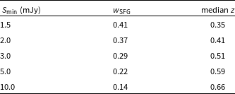
Redshift distributions after applying the flux threshold $S_{150}\!\ge\!1.5\,\mathrm{mJy}$
(Section 5.1). Top: total P(z) from GHOST (black). The green curve reconstructs the total as
$S_{150}\!\ge\!1.5\,\mathrm{mJy}$
(Section 5.1). Top: total P(z) from GHOST (black). The green curve reconstructs the total as $w_\mathrm{{SFG}}\,P_\mathrm{{SFG}}(z)+w_\mathrm{AGN}\,P_\mathrm{AGN}(z)$
using the intrinsic flux-limited class fractions
$w_\mathrm{{SFG}}\,P_\mathrm{{SFG}}(z)+w_\mathrm{AGN}\,P_\mathrm{AGN}(z)$
using the intrinsic flux-limited class fractions $(w_\mathrm{{SFG}},w_\mathrm{AGN})$
; the blue curve uses the same
$(w_\mathrm{{SFG}},w_\mathrm{AGN})$
; the blue curve uses the same $P_\mathrm{{SFG}}(z),P_\mathrm{AGN}(z)$
but reweights the class fractions by the acsLoTSS peak–S/N
$P_\mathrm{{SFG}}(z),P_\mathrm{AGN}(z)$
but reweights the class fractions by the acsLoTSS peak–S/N $\ge 7.5$
area acceptance from a log-normal rms model (
$\ge 7.5$
area acceptance from a log-normal rms model ( $\tilde{\sigma}=83\,\unicode{x03BC}\mathrm{Jy\,beam^{-1}}$
, 95th percentile
$\tilde{\sigma}=83\,\unicode{x03BC}\mathrm{Jy\,beam^{-1}}$
, 95th percentile $171\,\unicode{x03BC}\mathrm{Jy\,beam^{-1}}$
). The dashed line shows the acsLoTSS-DR2 parametric model. The green and blue reconstructions are essentially identical, indicating that the peak–S/N cut only weakly perturbs the class mix at 1.5 mJy. Middle/bottom: AGN and SFG PDFs (unit area) with medians and IQRs indicated. Relative to acsLoTSS, the simulated total places excess weight at
$171\,\unicode{x03BC}\mathrm{Jy\,beam^{-1}}$
). The dashed line shows the acsLoTSS-DR2 parametric model. The green and blue reconstructions are essentially identical, indicating that the peak–S/N cut only weakly perturbs the class mix at 1.5 mJy. Middle/bottom: AGN and SFG PDFs (unit area) with medians and IQRs indicated. Relative to acsLoTSS, the simulated total places excess weight at $z\!\lesssim\!0.4$
and underpowers the
$z\!\lesssim\!0.4$
and underpowers the $z\!\gtrsim\!0.6$
shoulder, suggesting a slightly SFG-heavy mix.
$z\!\gtrsim\!0.6$
shoulder, suggesting a slightly SFG-heavy mix.

After replicating the $1.5$
mJy sensitivity the selection function removes only a few percent of sources, so the resulting n(z) is driven by the intrinsic class mixture, shown in Figure 9. Where shown, the ‘LoTSS model’ is the parametric p(z) derived from Deep Fields. The total p(z) is low-z dominated (median
$1.5$
mJy sensitivity the selection function removes only a few percent of sources, so the resulting n(z) is driven by the intrinsic class mixture, shown in Figure 9. Where shown, the ‘LoTSS model’ is the parametric p(z) derived from Deep Fields. The total p(z) is low-z dominated (median $z=0.35$
, IQR
$z=0.35$
, IQR $0.15$
–
$0.15$
– $0.83$
), with a conspicuous SFG contribution at
$0.83$
), with a conspicuous SFG contribution at $z\lesssim0.3$
(SFG median
$z\lesssim0.3$
(SFG median $z=0.14$
, IQR
$z=0.14$
, IQR $0.09$
–
$0.09$
– $0.20$
). The AGN component peaks broadly around
$0.20$
). The AGN component peaks broadly around $z\sim0.5$
–1 (median
$z\sim0.5$
–1 (median $z=0.75$
, IQR
$z=0.75$
, IQR $0.47$
–
$0.47$
– $1.08$
). Using the measured 150 MHz counts-by-population to set the mixture yields
$1.08$
). Using the measured 150 MHz counts-by-population to set the mixture yields $w_\mathrm{{SFG}}\approx0.42$
. Figure 9 compares the resulting PDFs to the LoTSS model. Relative to the LoTSS model, the total median is lower and the high-z shoulder is underpowered, indicating a SFG-heavy mix at the mJy level and an under-representation of moderate-z AGNs in the total.
$w_\mathrm{{SFG}}\approx0.42$
. Figure 9 compares the resulting PDFs to the LoTSS model. Relative to the LoTSS model, the total median is lower and the high-z shoulder is underpowered, indicating a SFG-heavy mix at the mJy level and an under-representation of moderate-z AGNs in the total.
Increasing the flux cut shifts the prediction as expected (more AGN-dominated, higher median z), yet even at 10 mJy the median remains below the LoTSS curve (Table 6). The direction and size of the offset are consistent with the RLF diagnostics (Section 5.8); possible population-level origins are deferred to Section 5.6.
5.6.3. VLA-COSMOS split at 1.4 GHz
To mirror VLA-COSMOS (Magliocchetti et al. Reference Magliocchetti, Popesso, Brusa, Salvato, Laigle, McCracken and Ilbert2017), we apply a flux cut $F_{1.4}\ge0.15$
mJy and partition sources using a redshift-dependent luminosity boundary, as detailed in Section 5.1.
$F_{1.4}\ge0.15$
mJy and partition sources using a redshift-dependent luminosity boundary, as detailed in Section 5.1.
At $F_{1.4}\ge150\,\unicode{x03BC}\mathrm{Jy}$
the sample is still expected to contain a mixed population of radio-loud AGN and SFGs, that is, the selection lies in a transition regime rather than the more purely SFG-dominated depths
$F_{1.4}\ge150\,\unicode{x03BC}\mathrm{Jy}$
the sample is still expected to contain a mixed population of radio-loud AGN and SFGs, that is, the selection lies in a transition regime rather than the more purely SFG-dominated depths $\lesssim$ $100\,\unicode{x03BC}\mathrm{Jy}$
. In our framework this follows directly from the redshift-dependent luminosity threshold
$100\,\unicode{x03BC}\mathrm{Jy}$
. In our framework this follows directly from the redshift-dependent luminosity threshold $L_\mathrm{ lim}(z,\alpha)$
implied by a fixed flux limit:
$L_\mathrm{ lim}(z,\alpha)$
implied by a fixed flux limit: $L_\mathrm{lim}$
rises rapidly with z and progressively favours intrinsically luminous systems at
$L_\mathrm{lim}$
rises rapidly with z and progressively favours intrinsically luminous systems at $z\gtrsim1$
, which are typically AGN. For this reason, the population fractions inferred from the selected n(z) are expected to evolve with redshift, and we therefore report the predicted AGN/SFG fractions for this flux cut (both integrated and in broad redshift bins) and present the analogous assessment for the 150 MHz and 3 GHz selections.
$z\gtrsim1$
, which are typically AGN. For this reason, the population fractions inferred from the selected n(z) are expected to evolve with redshift, and we therefore report the predicted AGN/SFG fractions for this flux cut (both integrated and in broad redshift bins) and present the analogous assessment for the 150 MHz and 3 GHz selections.
VLA-COSMOS-like n(z) with 1.4 G Hz selection. We apply $F_{1.4}\!\ge\!0.15$
mJy and classify sources via
$F_{1.4}\!\ge\!0.15$
mJy and classify sources via $L_{1.4}\gtrless L_\mathrm{cross}(z)$
with
$L_{1.4}\gtrless L_\mathrm{cross}(z)$
with $L_\mathrm{cross}=4\pi P_\mathrm{cross}$
and
$L_\mathrm{cross}=4\pi P_\mathrm{cross}$
and $\log_{10}P_\mathrm{cross}(z)=21.7+z$
(
$\log_{10}P_\mathrm{cross}(z)=21.7+z$
( $z\!\le\!1.8$
) or
$z\!\le\!1.8$
) or $23.5$
otherwise (Section 5.1.2). Top: total P(z) with median and IQR; middle/bottom: AGN-like and SFG-like PDFs. The expected qualitative in redshift – with SFG tightly clustered and AGN more broad – is recovered, but the integrated SFG-like fraction is high, again pointing to a slightly SFG-heavy mix at the mJy level.
$23.5$
otherwise (Section 5.1.2). Top: total P(z) with median and IQR; middle/bottom: AGN-like and SFG-like PDFs. The expected qualitative in redshift – with SFG tightly clustered and AGN more broad – is recovered, but the integrated SFG-like fraction is high, again pointing to a slightly SFG-heavy mix at the mJy level.

The total resulting distribution, as shown in Figure 10 remains low-z dominated (median $z=0.37$
, IQR
$z=0.37$
, IQR $0.17$
–
$0.17$
– $0.87$
). The AGN-like PDF peaks at
$0.87$
). The AGN-like PDF peaks at $z\sim0.6$
–1 with a tail to
$z\sim0.6$
–1 with a tail to $z\sim2$
, while the SFG-like PDF is tightly concentrated at
$z\sim2$
, while the SFG-like PDF is tightly concentrated at $z\lesssim0.3$
. Integrating above/below
$z\lesssim0.3$
. Integrating above/below $L_\mathrm{cross}(z)$
gives an SFG fraction for this selection of
$L_\mathrm{cross}(z)$
gives an SFG fraction for this selection of
 \begin{equation}f_\mathrm{{SFG}} \equiv \frac{N_\mathrm{{SFG}}}{N_\mathrm{{SFG}}+N_\mathrm{AGN}} \;=\; 0.49 .\end{equation}
VLA–COSMOS-like n(z) at 3 GHz. GHOST total (top) and class PDFs (middle/bottom) for a $\mathrm{S/N}\!\ge\!5.5$
selection function (Section 5.1.3); the top panel also shows the effective counts-weighted mixture (green). Medians and IQRs are indicated. The total median is low and the SFG fraction is high compared to Hale et al. (Reference Hale, Jarvis, Delvecchio, Hatfield and Novak2018), consistent with the trend that GHOST overweights nearby SFG relative to moderate-z radio-loud AGN.
$\mathrm{S/N}\!\ge\!5.5$
selection function (Section 5.1.3); the top panel also shows the effective counts-weighted mixture (green). Medians and IQRs are indicated. The total median is low and the SFG fraction is high compared to Hale et al. (Reference Hale, Jarvis, Delvecchio, Hatfield and Novak2018), consistent with the trend that GHOST overweights nearby SFG relative to moderate-z radio-loud AGN.

The selection function recovers the expected qualitative separation in n(z) prevalent in Magliocchetti et al. (Reference Magliocchetti, Popesso, Brusa, Salvato, Laigle, McCracken and Ilbert2017), with SFG tightly clustered at low redshift and a broader AGN distribution, but the integrated SFG share is high for this selection, again pointing to a SFG-heavy mix around the mJy level. Because this diagnostic does not depend on peak-vs-integrated flux (unlike LoTSS), it isolates the population modelling: too many low-z SFG and/or too few moderate-z radio-loud AGNs.
Relative to the COSMOS-based fractions of (Magliocchetti et al. Reference Magliocchetti, Popesso, Brusa, Salvato, Laigle, McCracken and Ilbert2017), our $f_\mathrm{{SFG}}$
is larger in the same sense indicated by the LoTSS test. A hard L-threshold is an imperfect classifier (e.g. it can move luminous SFG at
$f_\mathrm{{SFG}}$
is larger in the same sense indicated by the LoTSS test. A hard L-threshold is an imperfect classifier (e.g. it can move luminous SFG at $z\sim1$
into the AGN-like bin), so exact numerical agreement is not expected; the direction of the difference is robust and consistent across selections.
$z\sim1$
into the AGN-like bin), so exact numerical agreement is not expected; the direction of the difference is robust and consistent across selections.
5.6.4. VLA-COSMOS-like selection at 3 GHz
We emulate the $\mathrm{S/N}\ge5.5$
3 GHz selection (median rms
$\mathrm{S/N}\ge5.5$
3 GHz selection (median rms $\simeq2.3\,\unicode{x03BC}$
Jy beam
$\simeq2.3\,\unicode{x03BC}$
Jy beam $^{-1}$
) and compare to the multi-wavelength SFG/AGN classes of Hale et al. (Reference Hale, Jarvis, Delvecchio, Hatfield and Novak2018).
$^{-1}$
) and compare to the multi-wavelength SFG/AGN classes of Hale et al. (Reference Hale, Jarvis, Delvecchio, Hatfield and Novak2018).
At the Hale et al. (Reference Hale, Jarvis, Delvecchio, Hatfield and Novak2018) depth the applied flux threshold and selection function detailed in Section 5.1 is weak: numerically the acceptances are close to unity for both classes (in our run $\mathrm{acc}_\mathrm{{SFG}}\!\approx\!0.89$
,
$\mathrm{acc}_\mathrm{{SFG}}\!\approx\!0.89$
, $\mathrm{acc}_\mathrm{AGN}\!\approx\!0.94$
), so the predicted n(z) is governed mainly by the intrinsic SFG/AGN mix. The total has median
$\mathrm{acc}_\mathrm{AGN}\!\approx\!0.94$
), so the predicted n(z) is governed mainly by the intrinsic SFG/AGN mix. The total has median $z=0.38$
. Class medians are
$z=0.38$
. Class medians are $z_\mathrm{med}^\mathrm{{SFG}}=0.30$
(IQR
$z_\mathrm{med}^\mathrm{{SFG}}=0.30$
(IQR $0.19$
–
$0.19$
– $0.45$
) and
$0.45$
) and $z_\mathrm{med}^\mathrm{AGN}=0.80$
(IQR
$z_\mathrm{med}^\mathrm{AGN}=0.80$
(IQR $0.48$
–
$0.48$
– $1.22$
). The effective SFG fraction is
$1.22$
). The effective SFG fraction is $w_\mathrm{{SFG}}=0.69$
.
$w_\mathrm{{SFG}}=0.69$
.
Normalised redshift PDFs under a MIGHTEE-like 1.4 GHz flux cut: GHOST (solid) compared to the MIGHTEE catalogue (dashed), shown for the total sample and AGN and SFG subsets. Vertical lines indicate medians (solid) and interquartile ranges (dashed).

At this depth and frequency the selection is intrinsically SFG-rich, but the simulated mixture is still somewhat SFG-heavy relative to Hale et al. (Reference Hale, Jarvis, Delvecchio, Hatfield and Novak2018), again implicating the population balance rather than the survey selection function. Hale et al. (Reference Hale, Jarvis, Delvecchio, Hatfield and Novak2018) classify $\sim$
79% of sources via multi-wavelength diagnostics and report a SFG share of
$\sim$
79% of sources via multi-wavelength diagnostics and report a SFG share of $\simeq$ $3\,704/3\,704+2\,937)\approx0.56$
in the masked field, together with a higher total median z (see their Figure 3). Our Hale-like selection therefore echoes the acsLoTSS and Magliocchetti results: GHOST places relatively more weight in nearby SFG and underweights moderate-z radio-loud AGN. The sign and scale of the difference are consistent with the RLF and clustering comparisons.
$3\,704/3\,704+2\,937)\approx0.56$
in the masked field, together with a higher total median z (see their Figure 3). Our Hale-like selection therefore echoes the acsLoTSS and Magliocchetti results: GHOST places relatively more weight in nearby SFG and underweights moderate-z radio-loud AGN. The sign and scale of the difference are consistent with the RLF and clustering comparisons.
5.6.5. MIGHTEE-like deep 1.4 GHz selection
Figure 12 compares the redshift PDFs obtained under the MIGHTEE-like cut to the GHOST catalogue, for the total sample and the AGN/SFG subsets. The deep cut produces the expected shift towards an SFG-dominated sample in GHOST: for $F_{1.4}\ge 8.5\,\unicode{x03BC}\mathrm{Jy}$
we find an effective SFG fraction of
$F_{1.4}\ge 8.5\,\unicode{x03BC}\mathrm{Jy}$
we find an effective SFG fraction of $f_\mathrm{{SFG}}=0.79$
(with the remaining
$f_\mathrm{{SFG}}=0.79$
(with the remaining $0.21$
in radio-loud AGNs). However, relative to the MIGHTEE distributions the simulated PDFs remain with excess low redshift SFG echoing the trend seen in Sections 5.6.2 and Sections 5.6.4 places excess weight in nearby SFGs and underweights moderate-z radio-loud AGN.
$0.21$
in radio-loud AGNs). However, relative to the MIGHTEE distributions the simulated PDFs remain with excess low redshift SFG echoing the trend seen in Sections 5.6.2 and Sections 5.6.4 places excess weight in nearby SFGs and underweights moderate-z radio-loud AGN.
5.7. Differential and Euclidean-normalised number counts
This section tests the total source density in GHOST against the literature via Euclidean-normalised differential counts, $S^{2.5}\,dN/dS$
, at 150 MHz, 1.4 GHz, and 3 GHz. Because number counts integrate over luminosity and redshift, they primarily probe the combination of luminosity-function normalisations and radio SEDs, largely independent of the host-halo assignment used for clustering.
$S^{2.5}\,dN/dS$
, at 150 MHz, 1.4 GHz, and 3 GHz. Because number counts integrate over luminosity and redshift, they primarily probe the combination of luminosity-function normalisations and radio SEDs, largely independent of the host-halo assignment used for clustering.
Figure 13 shows that over nearly seven decades in flux density the simulation follows the observed trends at all three frequencies. At the bright end ( $S\gtrsim10$
mJy), the counts are close to Euclidean (
$S\gtrsim10$
mJy), the counts are close to Euclidean ( $S^{2.5}\,dN/dS\!\approx\!\mathrm{const}$
), consistent with a population dominated by radio-loud AGN.
$S^{2.5}\,dN/dS\!\approx\!\mathrm{const}$
), consistent with a population dominated by radio-loud AGN.
Euclidean-normalised differential counts, $S^{2.5}\,{d}N/{d}S$
, for GHOST (black markers) compared to measurements at 150 MHz (Franzen et al. Reference Franzen2016; Mandal et al. Reference Mandal2021), 1.4 GHz (Bondi et al. Reference Bondi, Ciliegi and Schinnerer2008; Bridle et al. Reference Bridle, Davis, Fomalont and Lequeux1972; Ciardi & Loeb Reference Ciardi and Loeb2000; Fomalont et al. Reference Fomalont, Kellermann, Cowie, Capak, Barger, Partridge, Windhorst and Richards2006; Gruppioni et al. Reference Gruppioni, Mignoli and Zamorani1999; Hopkins et al. Reference Hopkins, Afonso, Chan, Cram, Georgakakis and Mobasher2003; Ibar et al. Reference Ibar, Ivison, Biggs, Lal, Best and Green2009; Kellermann et al. Reference Kellermann, Fomalont, Mainieri, Padovani, Rosati, Shaver, Tozzi and Miller2008; Mitchell & Condon Reference Mitchell and Condon1985; Owen & Morrison Reference Owen and Morrison2008; Richards Reference Richards2000; Seymour et al. Reference Seymour2008; White et al. Reference White, Becker, Helfand and Gregg1997; de Zotti et al. Reference de Zotti, Massardi, Negrello and Wall2010) and 3 GHz (Smol
$S^{2.5}\,{d}N/{d}S$
, for GHOST (black markers) compared to measurements at 150 MHz (Franzen et al. Reference Franzen2016; Mandal et al. Reference Mandal2021), 1.4 GHz (Bondi et al. Reference Bondi, Ciliegi and Schinnerer2008; Bridle et al. Reference Bridle, Davis, Fomalont and Lequeux1972; Ciardi & Loeb Reference Ciardi and Loeb2000; Fomalont et al. Reference Fomalont, Kellermann, Cowie, Capak, Barger, Partridge, Windhorst and Richards2006; Gruppioni et al. Reference Gruppioni, Mignoli and Zamorani1999; Hopkins et al. Reference Hopkins, Afonso, Chan, Cram, Georgakakis and Mobasher2003; Ibar et al. Reference Ibar, Ivison, Biggs, Lal, Best and Green2009; Kellermann et al. Reference Kellermann, Fomalont, Mainieri, Padovani, Rosati, Shaver, Tozzi and Miller2008; Mitchell & Condon Reference Mitchell and Condon1985; Owen & Morrison Reference Owen and Morrison2008; Richards Reference Richards2000; Seymour et al. Reference Seymour2008; White et al. Reference White, Becker, Helfand and Gregg1997; de Zotti et al. Reference de Zotti, Massardi, Negrello and Wall2010) and 3 GHz (Smol $\breve{c}$
ić et al. Reference Smolčić2017). Error bars are
$\breve{c}$
ić et al. Reference Smolčić2017). Error bars are $1\sigma$
measurement uncertainties, incorporating the estimations of Gehrels (Reference Gehrels1986) if
$1\sigma$
measurement uncertainties, incorporating the estimations of Gehrels (Reference Gehrels1986) if $N\lt20$
for any bin; shaded bands (if shown) indicate the field-to-field variance from GHOST mock realisations with the same area and flux cuts as the data. Residual panels show
$N\lt20$
for any bin; shaded bands (if shown) indicate the field-to-field variance from GHOST mock realisations with the same area and flux cuts as the data. Residual panels show $(\text{model}-\text{data})/\text{data}$
.
$(\text{model}-\text{data})/\text{data}$
.

A tension appears around the classical sub-mJy upturn, where the data rise due to the emergence of SFG. In our model this rise is weaker at $S\sim0.1$
–
$S\sim0.1$
– $0.3$
mJy. This behaviour is fully consistent with the adopted SFG RLF: the radio-first, smoothly evolving SFG luminosity function underpredicts the luminous tail of SFG at
$0.3$
mJy. This behaviour is fully consistent with the adopted SFG RLF: the radio-first, smoothly evolving SFG luminosity function underpredicts the luminous tail of SFG at $z\gtrsim1$
, which suppresses the upturn when projected to flux. Since total counts depend on the RLFs and SEDs rather than on host assignment, abundance matching does not drive this feature.
$z\gtrsim1$
, which suppresses the upturn when projected to flux. Since total counts depend on the RLFs and SEDs rather than on host assignment, abundance matching does not drive this feature.
5.7.1. Residuals
The residual panels plot $(\mathrm{model}/\mathrm{data})-1$
at the locations of the observational points. Away from the very faint and very bright limits, the residual clouds at 150 MHz, 1.4 GHz, and 3 GHz are centred on zero within the quoted errors, with a typical scatter of
$(\mathrm{model}/\mathrm{data})-1$
at the locations of the observational points. Away from the very faint and very bright limits, the residual clouds at 150 MHz, 1.4 GHz, and 3 GHz are centred on zero within the quoted errors, with a typical scatter of $\pm(10\text{-}30)\,\%$
across
$\pm(10\text{-}30)\,\%$
across $\sim4$
dex in S, indicating no frequency-dependent bias in the combination of RLFs and SEDs. Where residuals dip near the sub-mJy regime (most visibly at 1.4 GHz, with corresponding ranges at 150 MHz and 3 GHz), the shortfall follows from the SFG RLF’s high-L tail rather than from halo scarcity or assignment choices. At the brightest fluxes, excursions of order
$\sim4$
dex in S, indicating no frequency-dependent bias in the combination of RLFs and SEDs. Where residuals dip near the sub-mJy regime (most visibly at 1.4 GHz, with corresponding ranges at 150 MHz and 3 GHz), the shortfall follows from the SFG RLF’s high-L tail rather than from halo scarcity or assignment choices. At the brightest fluxes, excursions of order $\gtrsim$
30% reflect the rarity of luminous AGN and the small effective survey volumes of the anchoring datasets.
$\gtrsim$
30% reflect the rarity of luminous AGN and the small effective survey volumes of the anchoring datasets.
5.7.2. Implications
The close match to multi-frequency counts implies that the global normalisations of the luminosity functions, the adopted radio SEDs, and the applied survey selections are mutually consistent: GHOST produces the correct number of sources as a function of flux density without frequency-dependent bias, apart from the discussed SFG underprediction at the sub-mJy upturn. Because counts constrain the sum over populations, different SFG/AGN partitions can yield similar totals; discrepancies seen later in n(z), the RLFs, and clustering should therefore be interpreted as redistributions across populations and redshifts rather than a failure in the overall source density. The 3 GHz panel of Figure 13 shows the same behaviour, indicating that the spectral extrapolation from 1.4 to 3 GHz is consistent at the precision of current counts.
5.8. RLF
We describe the class-dependent RLF by $\Phi_c(L_\nu,z)$
in units of
$\Phi_c(L_\nu,z)$
in units of $\mathrm{Mpc}^{-3}\,\mathrm{dex}^{-1}$
, where
$\mathrm{Mpc}^{-3}\,\mathrm{dex}^{-1}$
, where $c\in\{\mathrm{SFG},\mathrm{SSAGN},\mathrm{FSRQ},\mathrm{BLLac}\}$
. Observed flux density at
$c\in\{\mathrm{SFG},\mathrm{SSAGN},\mathrm{FSRQ},\mathrm{BLLac}\}$
. Observed flux density at $\nu_\mathrm{obs}$
is related to rest-frame luminosity through the standard K-correction,
$\nu_\mathrm{obs}$
is related to rest-frame luminosity through the standard K-correction,
 \begin{equation} L_\nu(z,\alpha_c) = 4\pi D_L^2(z)\,S_{\nu_\mathrm{obs}}\, \Big(\frac{\nu_\mathrm{ref}}{\nu_\mathrm{obs}}\Big)^{-\alpha_c}(1+z)^{1+\alpha_c}, \end{equation}
so that, for a survey flux limit $S_\mathrm{lim}$
, the luminosity boundary within a redshift slice is
$S_\mathrm{lim}$
, the luminosity boundary within a redshift slice is
 \begin{equation} L_{\mathrm{lim}}(z,\alpha_c) = 4\pi D_L^2(z)\,S_{\mathrm{lim}}\, \Big(\frac{\nu_\mathrm{ref}}{\nu_\mathrm{obs}}\Big)^{-\alpha_c}(1+z)^{1+\alpha_c},\end{equation}
with $L_\nu\propto\nu^{-\alpha}$
.
$L_\nu\propto\nu^{-\alpha}$
.
Forward (projected) model. When comparing to data taken over a finite redshift bin $z\in[z_1,z_2]$
we project the intrinsic RLF under the same selection,
$z\in[z_1,z_2]$
we project the intrinsic RLF under the same selection,
 \begin{equation}\begin{aligned}v c&\Phi^\mathrm{proj}_c(L\,|\,z_1{:}z_2) = \\&\frac{\int_{z_1}^{z_2} \Phi_c(L,z)\, \Theta \big[L-L_\mathrm{lim}(z,\alpha_c)\big]\, ({{d}V}/{d}z)\,{d}z} {\int_{z_1}^{z_2} ({{d}V}/{d}z)\,{d}z} .\end{aligned}\end{equation}
These orange dashed curves in Figures 16 and 17 should be regarded as the baseline ‘model-to-data’ comparison.
Binned estimator from the catalogue ( $V_\mathrm{eff}$
). The blue points are a direct estimate from the catalogue in the
$V_\mathrm{eff}$
). The blue points are a direct estimate from the catalogue in the $[z_1,z_2]\times[L_1,L_2]$
cell using an effective volume that accounts for partial visibility of the L-bin across the slice. Define the bin width in dex by
$[z_1,z_2]\times[L_1,L_2]$
cell using an effective volume that accounts for partial visibility of the L-bin across the slice. Define the bin width in dex by $\Delta\log_{10}L=\log_{10}\!(L_2/L_1)$
. At any redshift z, the fraction of the luminosity bin that is observable is
$\Delta\log_{10}L=\log_{10}\!(L_2/L_1)$
. At any redshift z, the fraction of the luminosity bin that is observable is
 \begin{align}&f_\mathrm{vis}(z;\,L_1,L_2)= \nonumber \\[2pt] &\begin{cases}1 &L_\mathrm{lim}(z,\alpha_c)\le L_1,\\[2pt]\displaystyle\frac{\log_{10}\!\big(L_2/L_\mathrm{lim}(z,\alpha_c)\big)} {\log_{10}\!\big(L_2/L_1\big)} &L_1\lt L_\mathrm{lim}(z,\alpha_c) \lt L_2,\\[2pt]0 &L_\mathrm{lim}(z,\alpha_c)\ge L_2\, .\end{cases}\end{align}
Fraction of (L, z) cells with zero effective volume, $V_\mathrm{eff}=0$
, in each redshift bin for the raw selection. Bars show the average masked fraction across AGN and SFG classes; these are indistinguishable within
$V_\mathrm{eff}=0$
, in each redshift bin for the raw selection. Bars show the average masked fraction across AGN and SFG classes; these are indistinguishable within $\lesssim$ $0.5\%$
in every bin because the mask is set by the survey flux limit (and K-correction) rather than population physics. The fraction rises monotonically from
$0.5\%$
in every bin because the mask is set by the survey flux limit (and K-correction) rather than population physics. The fraction rises monotonically from $\lesssim$
15% at
$\lesssim$
15% at $z\le0.3$
to
$z\le0.3$
to $\simeq$
40% by
$\simeq$
40% by $z\sim1.8$
, reflecting the shrinking accessible luminosity range in a flux-limited survey. Cells with
$z\sim1.8$
, reflecting the shrinking accessible luminosity range in a flux-limited survey. Cells with $V_\mathrm{eff}=0$
are excluded from the panel-averaged RLFs.
$V_\mathrm{eff}=0$
are excluded from the panel-averaged RLFs.

The corresponding effective comoving volume for the cell is
 \begin{equation} V_\mathrm{eff}(L_1,L_2;\,z_1{:}z_2) \;=\; \Omega \int_{z_1}^{z_2} \frac{{d}V}{{d}z}(z)\, f_\mathrm{vis}(z;\,L_1,L_2)\,{d}z, \end{equation}
with survey solid angle $\Omega$
(sr). If
$\Omega$
(sr). If $N_c$
catalogue objects of class c fall in the cell, the minimum-variance, Poisson estimator is
$N_c$
catalogue objects of class c fall in the cell, the minimum-variance, Poisson estimator is
 \begin{align} \widehat{\Phi}_c(L\,|z_1{:}z_2) \; &=\; \frac{N_c}{V_\mathrm{eff}(L_1,L_2;\,z_1{:}z_2)\,\Delta\log_{10}L}\,, \\[-10pt] \nonumber \end{align}
 \begin{align} \sigma^2\!\left[\widehat{\Phi}_c\right] \;&=\; \frac{N_c}{\big[V_\mathrm{eff}\,\Delta\log_{10}L\big]^2}. \\[12pt] \nonumber \end{align}
If $N\lt20$
for any bin, we use the estimators of Gehrels (Reference Gehrels1986) in constructing the confidence interval. We plot the estimate at the bin centre with vertical error bars (from Equation 36) and omit bins where
$N\lt20$
for any bin, we use the estimators of Gehrels (Reference Gehrels1986) in constructing the confidence interval. We plot the estimate at the bin centre with vertical error bars (from Equation 36) and omit bins where $V_\mathrm{eff}=0$
. Horizontal bars indicate
$V_\mathrm{eff}=0$
. Horizontal bars indicate $\Delta\log_{10}L$
. For empty bins with
$\Delta\log_{10}L$
. For empty bins with $V_\mathrm{eff}\gt0$
we show one-sided upper limits (Gehrels-style) when useful.
$V_\mathrm{eff}\gt0$
we show one-sided upper limits (Gehrels-style) when useful.
Masked fraction of (
L
,
z
) cells. Figure 14 shows, for each redshift bin, the fraction of (L, z) cells that are masked because their effective survey volume is zero, $V_\mathrm{eff}(z,L)=0$
. A cell is masked precisely when the visibility fraction in Equation (33) vanishes,
$V_\mathrm{eff}(z,L)=0$
. A cell is masked precisely when the visibility fraction in Equation (33) vanishes, $f_\mathrm{vis}(z;\,L_1,L_2)=0$
; in those cells we set
$f_\mathrm{vis}(z;\,L_1,L_2)=0$
; in those cells we set $\Phi$
to NaN and exclude them from the RLF averages. As expected for a flux-limited sample, the masked fraction is
$\Phi$
to NaN and exclude them from the RLF averages. As expected for a flux-limited sample, the masked fraction is $\simeq 0$
in the nearest slice
$\simeq 0$
in the nearest slice $(0 \lt z\le0.1)$
and then rises monotonically with redshift as the flux boundary
$(0 \lt z\le0.1)$
and then rises monotonically with redshift as the flux boundary $L_\mathrm{lim}(z,\zeta)\propto D_L^2(z)\,(1+z)^{\zeta-1}$
moves to higher luminosities. Numerically, the fractions are
$L_\mathrm{lim}(z,\zeta)\propto D_L^2(z)\,(1+z)^{\zeta-1}$
moves to higher luminosities. Numerically, the fractions are $\approx$
15% at
$\approx$
15% at $0.10\text{-}0.30$
,
$0.10\text{-}0.30$
, $\approx$ $23\text{-}28\%$
at
$23\text{-}28\%$
at $0.30\text{-}0.70$
,
$0.30\text{-}0.70$
, $\approx$ $32\text{-}38\%$
at
$32\text{-}38\%$
at $0.70\text{-}1.40$
, and
$0.70\text{-}1.40$
, and $\approx$ $40\text{-}42\%$
by
$40\text{-}42\%$
by $z\simeq1.8$
. The AGN and SFG panels are nearly identical because the
$z\simeq1.8$
. The AGN and SFG panels are nearly identical because the $V_\mathrm{eff}$
mask is set by survey geometry and the adopted spectral index used in the visibility correction, not by population physics. Thus the increasing masked fraction simply quantifies the shrinking accessible L-range with redshift and explains the growing white space in the high-z RLF panels; it is a geometric selection effect, not a loss of simulated sources nor a model shortcoming.
$V_\mathrm{eff}$
mask is set by survey geometry and the adopted spectral index used in the visibility correction, not by population physics. Thus the increasing masked fraction simply quantifies the shrinking accessible L-range with redshift and explains the growing white space in the high-z RLF panels; it is a geometric selection effect, not a loss of simulated sources nor a model shortcoming.
Comparison of 1.4 GHz radio luminosity-SFR calibrations. Dashed curves show literature relations (Molnár et al. Reference Molnár2021; Heesen et al. Reference Heesen2022; Cook et al. Reference Cook2024; Matthews et al. Reference Matthews2024; Davies et al. Reference Davies2017; Murphy et al. Reference Murphy, Chary, Dickinson, Pope, Frayer and Lin2011; Bell et al. Reference Bell, McIntosh, Katz and Weinberg2003). The solid red line (‘this work’) is our adopted mapping. At high SFR the slope of our relation is shallower than several published fits, compressing the bright tail when mapping a given $\phi_\mathrm{ SFR}(z)$
into
$\phi_\mathrm{ SFR}(z)$
into $L_{1.4}$
and thereby yielding fewer SFG at
$L_{1.4}$
and thereby yielding fewer SFG at $L_{1.4}\!\gtrsim\!10^{23\text{-}24}\,\mathrm{W\,Hz^{-1}}$
. This behaviour contributes to the lower bright-end SFG space densities seen at
$L_{1.4}\!\gtrsim\!10^{23\text{-}24}\,\mathrm{W\,Hz^{-1}}$
. This behaviour contributes to the lower bright-end SFG space densities seen at $z\gtrsim1$
in Figure 17. The halo mass range and abundance matching limits the upper SFR range in practice.
$z\gtrsim1$
in Figure 17. The halo mass range and abundance matching limits the upper SFR range in practice.

AGN radio luminosity functions at 1.4 GHz in redshift slices (raw cut). Each panel shows $\Phi(L_\nu)\,(\mathrm{Mpc}^{-3}\,\mathrm{dex}^{-1})$
for the stated redshift bin. Blue circles: RLF measured from the simulation using the effective-volume method,
$\Phi(L_\nu)\,(\mathrm{Mpc}^{-3}\,\mathrm{dex}^{-1})$
for the stated redshift bin. Blue circles: RLF measured from the simulation using the effective-volume method, $\Phi = N/(V_\mathrm{eff}\,\Delta\log_{10}L)$
, where
$\Phi = N/(V_\mathrm{eff}\,\Delta\log_{10}L)$
, where $V_\mathrm{eff}$
accounts for the flux limit within the bin (Section 5.8; Equation 36). Error bars are
$V_\mathrm{eff}$
accounts for the flux limit within the bin (Section 5.8; Equation 36). Error bars are $1\sigma$
Poisson uncertainties propagated through
$1\sigma$
Poisson uncertainties propagated through $V_\mathrm{eff}$
; cells with
$V_\mathrm{eff}$
; cells with $V_\mathrm{eff}=0$
are omitted. Purple dashed: forward (projected) model
$V_\mathrm{eff}=0$
are omitted. Purple dashed: forward (projected) model $\Phi^\mathrm{proj}(L|z_1:z_2)$
obtained by averaging the intrinsic AGN RLF over the finite
$\Phi^\mathrm{proj}(L|z_1:z_2)$
obtained by averaging the intrinsic AGN RLF over the finite $\Delta z$
of the panel under the same flux selection (Equation 32). Points in the background: literature measurements at 1.4 GHz (legend in the top-left panel). Across the ten slices the simulation (blue) and the forward model (purple) show excellent agreement in both normalisation and shape; a mild feature near
$\Delta z$
of the panel under the same flux selection (Equation 32). Points in the background: literature measurements at 1.4 GHz (legend in the top-left panel). Across the ten slices the simulation (blue) and the forward model (purple) show excellent agreement in both normalisation and shape; a mild feature near $L_\nu\!\sim\!10^{26}\,\mathrm{W\,Hz^{-1}}$
reflects the combined contribution of flat-spectrum (FSRQ/BLLac) and steep-spectrum (SSAGN) components with luminosity-dependent evolution (see Section 5.8). Axis limits in each panel are set by the extent of the observational points to aid readability: Squares indicate radio loud AGN; diamonds indicate radio quiet AGN. Filled markers are fully within the z-bin; open markers partially overlap the bin.
$L_\nu\!\sim\!10^{26}\,\mathrm{W\,Hz^{-1}}$
reflects the combined contribution of flat-spectrum (FSRQ/BLLac) and steep-spectrum (SSAGN) components with luminosity-dependent evolution (see Section 5.8). Axis limits in each panel are set by the extent of the observational points to aid readability: Squares indicate radio loud AGN; diamonds indicate radio quiet AGN. Filled markers are fully within the z-bin; open markers partially overlap the bin.

SFG radio luminosity functions at 1.4 GHz in redshift slices (raw cut). As in the AGN figure, blue circles show the simulation RLF recovered with the effective-volume estimator $\Phi=N/(V_\mathrm{eff}\,\Delta\log_{10}L)$
(with
$\Phi=N/(V_\mathrm{eff}\,\Delta\log_{10}L)$
(with $1\sigma$
Poisson errors), and orange dashed curves are the forward (projected) model evaluated over the same
$1\sigma$
Poisson errors), and orange dashed curves are the forward (projected) model evaluated over the same $\Delta z$
and flux selection. Background points: literature measurements at 1.4 GHz (legend in the top-left panel). At
$\Delta z$
and flux selection. Background points: literature measurements at 1.4 GHz (legend in the top-left panel). At $z\!\lesssim\!1$
the model and simulation track the observed faint end well. At higher redshift the bright tail in the simulation/model sits below some compilations: this follows naturally from our adopted L-SFR mapping (shallower high-SFR slope), the tightening luminosity threshold imposed by the flux limit within each
$z\!\lesssim\!1$
the model and simulation track the observed faint end well. At higher redshift the bright tail in the simulation/model sits below some compilations: this follows naturally from our adopted L-SFR mapping (shallower high-SFR slope), the tightening luminosity threshold imposed by the flux limit within each $\Delta z$
slice, and the resulting reduction of accessible high-SFR systems (see Section 5.8). As before, panel limits are set by the extent of the observational points; filled markers are fully within the z-bin; open markers partially overlap the bin.
$\Delta z$
slice, and the resulting reduction of accessible high-SFR systems (see Section 5.8). As before, panel limits are set by the extent of the observational points; filled markers are fully within the z-bin; open markers partially overlap the bin.

Results at $\boldsymbol{1.4}$
GHz. Figures 16 and 17 show excellent agreement between the projected model (orange dashed) and the catalogue-based,
$\boldsymbol{1.4}$
GHz. Figures 16 and 17 show excellent agreement between the projected model (orange dashed) and the catalogue-based, $V_\mathrm{eff}$
-corrected estimates (blue points):
$V_\mathrm{eff}$
-corrected estimates (blue points):
-
• AGN: The match is tight across all redshift slices and over the full dynamic range where the survey is complete. This validates both the evolutionary form of the AGN RLF and the class mix encoded in the model.
-
• SFG: At
$z\gtrsim 1$
the blue points fall below some literature bright-end measurements. This is a model outcome: our adopted
$L_{1.4}$
–SFR calibration is shallower at high SFR (see Figure 15), compressing the bright tail and yielding fewer
$L_{1.4}\gtrsim 10^{23{-}24}\,\mathrm{W\,Hz^{-1}}$
systems when an evolving SFR function is mapped into radio luminosity. The same behaviour is consistent with the divergence of the total counts at the faint flux end where SFG dominate.



A shallow ‘bump/inflection’ occasionally visible in the orange curves near $10^{26}\,\mathrm{W\,Hz^{-1}}$
is naturally produced by the sum of AGN subclasses and their evolution; the double-power-law knee of the steep-spectrum tail, combined with the beamed (FSRQ/BLLac) component beginning to dominate the bright end with a slightly flatter local slope, and the finite-width slice average in Equation (32). A per-class decomposition of
$10^{26}\,\mathrm{W\,Hz^{-1}}$
is naturally produced by the sum of AGN subclasses and their evolution; the double-power-law knee of the steep-spectrum tail, combined with the beamed (FSRQ/BLLac) component beginning to dominate the bright end with a slightly flatter local slope, and the finite-width slice average in Equation (32). A per-class decomposition of $\Phi^\mathrm{proj}$
confirms that the total slope locally reflects the crossover of SSAGN and beamed contributions. The feature is therefore not required by the data and does not affect the excellent overall agreement.
$\Phi^\mathrm{proj}$
confirms that the total slope locally reflects the crossover of SSAGN and beamed contributions. The feature is therefore not required by the data and does not affect the excellent overall agreement.
5.9. The effect of observational parameters
The results discussed in this work use the GHOST intrinsic catalogue prior to applying survey-specific observational effects. In real radio-continuum analyses, going from an intrinsic sky to a detected catalogue depends on the synthesised beam, imaging/source-finding choices, and the confusion environment, which vary between instruments and releases; we therefore treat a fully general observational model as future work, and here summarise the main consequences of its omission.
5.9.1. Beam width
A finite beam smooths the sky brightness field and suppresses clustering on scales comparable to and below the beam (Peebles Reference Peebles1980; Condon Reference Condon1992; Hale et al. Reference Hale, Jarvis, Delvecchio, Hatfield and Novak2018). In source catalogues, finite resolution can also introduce resolution bias under peak-S/N selection, preferentially missing extended sources at fixed integrated flux and thereby modifying both the faint-end number counts and the effective redshift distribution of a selected sample (e.g. Bondi et al. Reference Bondi, Ciliegi and Schinnerer2008). Confusion and blending further perturb flux measurements and merge close pairs, distorting ${d}N/{d}S$
near the flux limit and suppressing small-scale clustering; catalogue-level component association can likewise bias close-pair counts by merging or splitting multi-component systems (e.g. Condon Reference Condon1992; Bondi et al. Reference Bondi, Ciliegi and Schinnerer2008; Hale et al. Reference Hale, Jarvis, Delvecchio, Hatfield and Novak2018).
${d}N/{d}S$
near the flux limit and suppressing small-scale clustering; catalogue-level component association can likewise bias close-pair counts by merging or splitting multi-component systems (e.g. Condon Reference Condon1992; Bondi et al. Reference Bondi, Ciliegi and Schinnerer2008; Hale et al. Reference Hale, Jarvis, Delvecchio, Hatfield and Novak2018).
Our angular-space fits use $\theta \in [0.02^\circ,0.5^\circ]$
(i.e.
$\theta \in [0.02^\circ,0.5^\circ]$
(i.e. $\gtrsim$
72 arcsec), and our harmonic-space fits focus on large scales (e.g.
$\gtrsim$
72 arcsec), and our harmonic-space fits focus on large scales (e.g. $\ell \in [40,250]$
), which are far larger than the synthesised beams of the surveys we emulate. The LoTSS-DR2 wide-area products are commonly analysed at
$\ell \in [40,250]$
), which are far larger than the synthesised beams of the surveys we emulate. The LoTSS-DR2 wide-area products are commonly analysed at $\sim$
6 arcsec resolution (Shimwell et al. Reference Shimwell2022), the VLA-COSMOS 1.4 GHz Large Project at
$\sim$
6 arcsec resolution (Shimwell et al. Reference Shimwell2022), the VLA-COSMOS 1.4 GHz Large Project at $\sim$ $1.5$
arcsec (Magliocchetti et al. Reference Magliocchetti, Popesso, Brusa, Salvato, Laigle, McCracken and Ilbert2017), and the VLA-COSMOS 3 GHz Large Project at
$1.5$
arcsec (Magliocchetti et al. Reference Magliocchetti, Popesso, Brusa, Salvato, Laigle, McCracken and Ilbert2017), and the VLA-COSMOS 3 GHz Large Project at $\sim$ $0.75$
arcsec (Hale et al. Reference Hale, Jarvis, Delvecchio, Hatfield and Novak2018). Consequently, beam smoothing primarily affects separations orders of magnitude smaller than those driving our large-scale clustering and bias comparisons. At the scales shown here, the dominant pathway for instrumental effects to enter is via sample selection, which we explicitly mirror for each survey, including modelling spatially varying rms for the LoTSS-DR2 selection. We therefore expect the principal conclusions of this work - that selection can control the projected clustering amplitude and slope through changes in n(z), while preserving the intrinsic bias ordering between populations – to be robust to the omission of an explicit modelling.
$0.75$
arcsec (Hale et al. Reference Hale, Jarvis, Delvecchio, Hatfield and Novak2018). Consequently, beam smoothing primarily affects separations orders of magnitude smaller than those driving our large-scale clustering and bias comparisons. At the scales shown here, the dominant pathway for instrumental effects to enter is via sample selection, which we explicitly mirror for each survey, including modelling spatially varying rms for the LoTSS-DR2 selection. We therefore expect the principal conclusions of this work - that selection can control the projected clustering amplitude and slope through changes in n(z), while preserving the intrinsic bias ordering between populations – to be robust to the omission of an explicit modelling.
5.9.2. Number counts and completeness near the detection limit
For catalogues selected at a peak-S/N threshold, extended sources of a given integrated flux density can fall below the peak-flux detection threshold more readily than compact sources, reducing completeness in the faintest bins (e.g. Bondi et al. Reference Bondi, Ciliegi and Schinnerer2008; Smol $\breve{c}$
ić et al. Reference Smolčić2017). Close to the survey limit, noise and confusion can scatter sources across a flux threshold, leading to Eddington bias (Eddington Reference Eddington1913), while blending can distort
$\breve{c}$
ić et al. Reference Smolčić2017). Close to the survey limit, noise and confusion can scatter sources across a flux threshold, leading to Eddington bias (Eddington Reference Eddington1913), while blending can distort ${d}N/{d}S$
by depleting faint bins and populating brighter bins (e.g. Condon Reference Condon1992). Published number counts are typically corrected for such survey-specific selection effects (e.g. incompleteness, resolution bias, and flux boosting), so like-for-like comparisons are best made either in flux ranges that are effectively complete or using counts that have been corrected for completeness in the same way. The counts used for our validation span a wide flux range and are compared primarily where the surveys are close to complete, so these effects are not expected to change the conclusions of this analysis.
${d}N/{d}S$
by depleting faint bins and populating brighter bins (e.g. Condon Reference Condon1992). Published number counts are typically corrected for such survey-specific selection effects (e.g. incompleteness, resolution bias, and flux boosting), so like-for-like comparisons are best made either in flux ranges that are effectively complete or using counts that have been corrected for completeness in the same way. The counts used for our validation span a wide flux range and are compared primarily where the surveys are close to complete, so these effects are not expected to change the conclusions of this analysis.
5.10. Impact of SFG modelling choices
The impact of alternative SFG modelling choices on number counts is quantified through two cross-checks: an IR-calibrated construction used to derive an effective radio RLF, and the inclusion of thermal dust emission as an SED component when generating multi-frequency fluxes (Section 3.2.1).
Figures 22–23 compare the redshift and flux distributions predicted by the IR-calibrated construction (Appendix A.7) against the fiducial radio-calibrated prescription. Over the redshift range where most SFGs contributing to typical radio selections lie ( $z\lesssim 2$
), the two constructions yield broadly similar N(z) and N(S) shapes, with differences at the factor-of-few level that decrease with redshift. The dominant qualitative difference is the high-redshift behaviour: in the tested IR-calibrated prescription the SFG density turns over more sharply at
$z\lesssim 2$
), the two constructions yield broadly similar N(z) and N(S) shapes, with differences at the factor-of-few level that decrease with redshift. The dominant qualitative difference is the high-redshift behaviour: in the tested IR-calibrated prescription the SFG density turns over more sharply at $z\gtrsim 3$
–4, whereas the radio-calibrated model retains a higher high-z tail. This behaviour reflects the fact that the IR-calibrated construction inherits assumptions about IR luminosity evolution and the IR-radio mapping (Yun et al. Reference Yun, Reddy and Condon2001; Cai et al. Reference Cai2013), while the fiducial GHOST model is explicitly calibrated to radio observables.
$z\gtrsim 3$
–4, whereas the radio-calibrated model retains a higher high-z tail. This behaviour reflects the fact that the IR-calibrated construction inherits assumptions about IR luminosity evolution and the IR-radio mapping (Yun et al. Reference Yun, Reddy and Condon2001; Cai et al. Reference Cai2013), while the fiducial GHOST model is explicitly calibrated to radio observables.
Figure 25 quantifies the effect of adding thermal dust emission as an SED component (Appendix A.7) on SFG number counts at high observing frequency. Across most redshifts the impact on N(z) is negligible, consistent with synchrotron/free-free dominating the SFG spectrum below $\sim$
10–20 GHz (Appendix A.6). In Bonaldi et al. (Reference Bonaldi, Bonato, Galluzzi, Harrison, Massardi, Kay, De Zotti and Brown2019), the rest-frame SFG SED is dust-dominated only at
$\sim$
10–20 GHz (Appendix A.6). In Bonaldi et al. (Reference Bonaldi, Bonato, Galluzzi, Harrison, Massardi, Kay, De Zotti and Brown2019), the rest-frame SFG SED is dust-dominated only at $\nu \gtrsim 100$
GHz, implying that dust becomes important in the observer frame only at frequencies of a few tens of GHz for high-redshift galaxies; they implement this by adding dust emission using the model of Cai et al. (Reference Cai2013) and the same SFR-
$\nu \gtrsim 100$
GHz, implying that dust becomes important in the observer frame only at frequencies of a few tens of GHz for high-redshift galaxies; they implement this by adding dust emission using the model of Cai et al. (Reference Cai2013) and the same SFR- $L_\mathrm{{IR}}$
calibration. Our results follow the same trend: the dust term affects only the extreme high-z tail at the highest frequencies, where the observer-frame band probes substantially higher rest-frame frequencies and the modified blackbody emission rises rapidly.
$L_\mathrm{{IR}}$
calibration. Our results follow the same trend: the dust term affects only the extreme high-z tail at the highest frequencies, where the observer-frame band probes substantially higher rest-frame frequencies and the modified blackbody emission rises rapidly.
This conclusion is also consistent with (Wilman et al. Reference Wilman2008), which adopts a modified blackbody dust component with $(T,\beta)=(45\,\mathrm{K},1.5)$
normalised via the IR-radio correlation and finds a discernible impact on the observed SED only at very high redshift and at the highest output frequency. For the metre-centimetre regimes emphasised in this work, omitting thermal dust emission therefore has negligible impact on the reported results, while including it improves SED completeness for multi-frequency catalogues.
$(T,\beta)=(45\,\mathrm{K},1.5)$
normalised via the IR-radio correlation and finds a discernible impact on the observed SED only at very high redshift and at the highest output frequency. For the metre-centimetre regimes emphasised in this work, omitting thermal dust emission therefore has negligible impact on the reported results, while including it improves SED completeness for multi-frequency catalogues.
6. Luminosity-redshift distributions by class
Figures 18–21 show, for each population, the distribution of rest-frame radio luminosity versus redshift. Shading encodes the relative number density per redshift bin; over-plotted are the median and mean of $\log_{10}L$
, central (p16–p84) and extended (p05–p95) percentile bands, and the minimum/maximum values realised in the catalogue. These panels are intended to summarise, at a glance, how the RLF and the survey selection combine to populate the light-cone for each class.
$\log_{10}L$
, central (p16–p84) and extended (p05–p95) percentile bands, and the minimum/maximum values realised in the catalogue. These panels are intended to summarise, at a glance, how the RLF and the survey selection combine to populate the light-cone for each class.
BLLac – luminosity distribution vs. redshift. Rows are normalised by their own maxima; ribbons show p16–p84 and p05–p95 of $\log_{10}L_\nu$
. The narrowing and softening of the upper envelope (shown by the dashed purple line) at high z reflect the flux limit and declining BL Lac space density. The lower minimum envelope is shown by the lower dashed line.
$\log_{10}L_\nu$
. The narrowing and softening of the upper envelope (shown by the dashed purple line) at high z reflect the flux limit and declining BL Lac space density. The lower minimum envelope is shown by the lower dashed line.

FSRQ – luminosity distribution vs. redshift. Same notation as 18. The broad luminous tail at $z\!\lesssim\!1$
and the subsequent contraction beyond
$z\!\lesssim\!1$
and the subsequent contraction beyond $z\!\sim\!3$
are evident.
$z\!\sim\!3$
are evident.

SSAGN – luminosity distribution vs. redshift. Same notation as 18. The median rises to $z\!\sim\!1$
and then turns over, with the distribution tightening as the flux boundary dominates.
$z\!\sim\!1$
and then turns over, with the distribution tightening as the flux boundary dominates.

SFG – luminosity distribution vs. redshift. Same notation as 18. The median follows the cosmic growth of typical SFRs to $z\!\sim\!2$
–3 and declines gently thereafter; the accessible upper envelope drops beyond
$z\!\sim\!2$
–3 and declines gently thereafter; the accessible upper envelope drops beyond $z\!\sim\!3$
as the flux limit and host availability restrict very luminous SFG.
$z\!\sim\!3$
as the flux limit and host availability restrict very luminous SFG.

IR-calibrated versus radio-calibrated SFG predictions: N(S) summed over redshift.

IR-calibrated versus radio-calibrated SFG predictions: N(z) summed over flux bins.

A few general features are common to all panels. The lower envelope follows the flux-limited luminosity threshold $L_\mathrm{lim}(z,\zeta)$
implied by the selection and K-corrections (Section 5.1), which rises rapidly with redshift and produces the Malmquist-like increase of the median at low z. The separation between the mean and the median indicates positive skewness due to a high-L tail; the width of the percentile bands traces the intrinsic luminosity spread convolved with selection. At
$L_\mathrm{lim}(z,\zeta)$
implied by the selection and K-corrections (Section 5.1), which rises rapidly with redshift and produces the Malmquist-like increase of the median at low z. The separation between the mean and the median indicates positive skewness due to a high-L tail; the width of the percentile bands traces the intrinsic luminosity spread convolved with selection. At $z\lesssim0.5$
the accessible dynamic range in L is largest and the bands are widest. As z increases the faint end is progressively removed by
$z\lesssim0.5$
the accessible dynamic range in L is largest and the bands are widest. As z increases the faint end is progressively removed by $L_\mathrm{lim}$
, the median rises, and the bright tail is governed by the evolving knee of the RLF and by the rarity of very luminous sources. Beyond
$L_\mathrm{lim}$
, the median rises, and the bright tail is governed by the evolving knee of the RLF and by the rarity of very luminous sources. Beyond $z\sim2$
–3 the high-L tail thins and the percentile bands narrow as space densities decline; small-number statistics appear as occasional spikes in the dotted ‘max’ curves in the highest-z bins.
$z\sim2$
–3 the high-L tail thins and the percentile bands narrow as space densities decline; small-number statistics appear as occasional spikes in the dotted ‘max’ curves in the highest-z bins.
IR-calibrated versus radio-calibrated SFG predictions: ratio of IR-calibrated to radio-calibrated N(z). The two prescriptions are similar for $z\lesssim 2$
, while the tested IR-calibrated prescription exhibits a steeper decline at high redshift.
$z\lesssim 2$
, while the tested IR-calibrated prescription exhibits a steeper decline at high redshift.

SFGs exhibit the lowest median luminosities and comparatively narrow percentile bands at fixed z. The median increases gently with redshift, while the mean sits only slightly above it, signalling limited skewness. The density shading peaks at intermediate redshift and fades by $z\sim3$
, consistent with the smoothly evolving, radio-first SFG RLF of Section 3.2. This behaviour also explains the modest sub-mJy upturn in the counts (Section 5.7): the high-L SFG tail at
$z\sim3$
, consistent with the smoothly evolving, radio-first SFG RLF of Section 3.2. This behaviour also explains the modest sub-mJy upturn in the counts (Section 5.7): the high-L SFG tail at $z\gtrsim1$
is present but not dominant, so the projected rise in
$z\gtrsim1$
is present but not dominant, so the projected rise in $S^{2.5}dN/dS$
is weaker than in datasets whose SFG bright end is steeper or more numerous.
$S^{2.5}dN/dS$
is weaker than in datasets whose SFG bright end is steeper or more numerous.
Steep-spectrum AGN span a wide luminosity range. Through $z\sim1$
–2 the high-L tail is prominent, lifting the mean well above the median and widening the p16–p84 band. The median sits roughly a dex above the SFG median at the same redshift, reflecting the higher typical host masses of radio-loud systems (Section 3.3). At
$z\sim1$
–2 the high-L tail is prominent, lifting the mean well above the median and widening the p16–p84 band. The median sits roughly a dex above the SFG median at the same redshift, reflecting the higher typical host masses of radio-loud systems (Section 3.3). At $z\gtrsim2.5$
the percentile bands narrow and the maximum realised luminosity drops, tracing both the SSAGN RLF evolution and the diminishing supply of massive halos available to host them (Section 4).
$z\gtrsim2.5$
the percentile bands narrow and the maximum realised luminosity drops, tracing both the SSAGN RLF evolution and the diminishing supply of massive halos available to host them (Section 4).
Flat-spectrum subclasses show the highest luminosities at fixed redshift. FSRQ display broad percentile bands and a large mean–median gap, as expected for a beamed population with a strong bright tail; the shading peaks around $z\sim1$
–2 and declines rapidly by
$z\sim1$
–2 and declines rapidly by $z\gtrsim3$
as the combination of RLF evolution and beamed fractions reduces the space density. BL Lac objects occupy a lower-luminosity locus than FSRQ and a somewhat narrower redshift span; their bands are tighter and the shading is more local-heavy, indicating milder evolution and smaller overall abundance. In both beamed classes the dotted ‘max’ curve shows occasional excursions at high redshift that are consistent with small-number statistics.
$z\gtrsim3$
as the combination of RLF evolution and beamed fractions reduces the space density. BL Lac objects occupy a lower-luminosity locus than FSRQ and a somewhat narrower redshift span; their bands are tighter and the shading is more local-heavy, indicating milder evolution and smaller overall abundance. In both beamed classes the dotted ‘max’ curve shows occasional excursions at high redshift that are consistent with small-number statistics.
These shapes have direct consequences for selection and for the observables compared elsewhere in this paper. Because changes in survey selection functions compress or broaden the effective redshift kernel $\varphi(z)$
(Section 5.1), the rising
$\varphi(z)$
(Section 5.1), the rising $L_\mathrm{lim}(z)$
cuts different parts of each panel for a given flux limit. SFG are most affected at low to intermediate redshift where their locus lies close to
$L_\mathrm{lim}(z)$
cuts different parts of each panel for a given flux limit. SFG are most affected at low to intermediate redshift where their locus lies close to $L_\mathrm{lim}$
; SSAGN and flat-spectrum AGN remain visible to higher z but are shot-noise limited in the brightest tail. This selection geometry explains why projected clustering amplitudes and slopes shift with the survey selection functions (Section 5.3) without altering the intrinsic bias ordering inferred from the host-mass distributions: SFG occupy lower-mass halos and populate lower L at a given z; SSAGN are intermediate; FSRQ/BL Lac trace the luminous, highly biased tail.
$L_\mathrm{lim}$
; SSAGN and flat-spectrum AGN remain visible to higher z but are shot-noise limited in the brightest tail. This selection geometry explains why projected clustering amplitudes and slopes shift with the survey selection functions (Section 5.3) without altering the intrinsic bias ordering inferred from the host-mass distributions: SFG occupy lower-mass halos and populate lower L at a given z; SSAGN are intermediate; FSRQ/BL Lac trace the luminous, highly biased tail.
For multi-tracer applications the panels make explicit that each class supplies a distinct P(z) kernel and linear-bias evolution. The ordered rise of the medians and the class-to-class offsets stabilise the bias contrast required for cosmic-variance cancellation on ultra-large scales, while the thinning of the bright tails at $z\gtrsim3$
sets practical limits on how aggressively very-high-z selections can be pushed before shot noise dominates. Together with the number-count agreement in Section 5.7 and the clustering results in Section 5.3, these luminosity-redshift maps close the loop between population prescriptions, host assignment, and the survey selections used for validation.
$z\gtrsim3$
sets practical limits on how aggressively very-high-z selections can be pushed before shot noise dominates. Together with the number-count agreement in Section 5.7 and the clustering results in Section 5.3, these luminosity-redshift maps close the loop between population prescriptions, host assignment, and the survey selections used for validation.
The effect of adding thermal dust emission as an SED component for SFGs at high observing frequency. Shown is N(z) for the fiducial radio-calibrated SFG population with and without the dust term. The impact is negligible at most redshifts and becomes noticeable only in the extreme high-z tail, where the observer-frame band probes higher rest-frame frequencies.

7. Improvements
GHOST is an all-sky radio-continuum simulation with population-dependent clustering, redshift distributions, and survey selections designed to emulate realistic wide-area datasets. Below we summarise where the current release is most useful and outline focused directions that will make it more powerful for cosmology and survey work.
-
• Spectral assumptions and K-corrections. Using a single (or overly narrow) spectral-index model per population tightens the flux-luminosity mapping, especially at high z where rest-frame frequencies shift. Future direction: adopt redshift-dependent spectral-index distributions (optionally with curvature), for exact downstream K-corrections, and validate against multi-frequency counts.
-
• SFG RLF bright end and the sub-mJy upturn. The radio-first SFG RLF underpredicts the high-L SFG tail at
$z\gtrsim1$
, weakening the classical upturn near
$S\sim0.1$
–
$0.3$
mJy. Future direction: re-fit the SFG RLF with deeper fields and include a cross-check pathway that links to SFR/IR constraints (without making them mandatory) to control the bright tail while preserving the radio-first baseline. -
• Satellites and halo occupation. The current catalogue assigns one central per halo and no explicit satellites. This can bias small-scale
$w(\theta)$
and environment trends, even if large-scale bias is stable. Future direction: add a minimal HOD layer (central + satellites) per population, tuned to small-scale clustering while keeping the ultra-large-scale predictions unchanged. -
• Survey realism and detection. Point-like components and simplified morphologies miss PSF/blending effects and spatially varying completeness. Future direction: ship an ‘observe-at-beam’ operator (beam, mosaics, noise/rms maps, deblending/thresholding) that produces detection catalogues, randoms, and effective-area curves consistent with pseudo-
$C_\ell$
inputs. -
• Documentation and delivered products. Future direction: include per-source SED parameters (
$\zeta$
, curvature), p(z) options, masks/randoms, and n(z) kernels used in the figures so analyses can be reproduced exactly.


Taken together, these items indicate where GHOST can grow. They also clarify how to interpret the current results: robust for wide-area cosmology under the stated assumptions, with clear paths to refine high-z populations, spectral modelling, morphology, and survey realism in future releases.
8. Conclusions
GHOST is an all-sky, clustered, survey-ready radio mock built on the flamingo light-cone and tailored to ultra-large-scale, multi-tracer cosmology. The catalogue ties population prescriptions to a specific halo field through rank-preserving, no-replacement abundance matching (Section 4), ensuring that large-scale bias follows the halo supply. The SFG branch is calibrated directly in radio via a smoothly evolving 1.4 GHz RLF (Section 3.2), while the AGN branch retains the t-recs functional form with coefficients refit as needed and a new host assignment on our light-cone (Section 3.3). Together these choices provide transparent control of bias and redshift kernels at the scales relevant for $f_\mathrm{NL}$
.
$f_\mathrm{NL}$
.
Across 150 MHz, 1.4 GHz, and 3 GHz the Euclidean-normalised differential counts are reproduced over nearly seven decades in flux (Section 5.7). The model shows no frequency-dependent bias in the total counts; the subdued sub-mJy upturn is consistent with the high-luminosity tail of the radio-first SFG RLF at $z\gtrsim1$
, rather than with host-assignment choices. This anchors the overall normalisation of the luminosity functions and spectral assumptions used throughout.
$z\gtrsim1$
, rather than with host-assignment choices. This anchors the overall normalisation of the luminosity functions and spectral assumptions used throughout.
Using common selections for both n(z) and clustering, we emulate the survey selection functions used by representative surveys and recover their qualitative behaviour (Section 5.6). Emulating acsLoTSS-wide, the VLA–COSMOS luminosity split of Magliocchetti et al. (Reference Magliocchetti, Popesso, Brusa, Salvato, Laigle, McCracken and Ilbert2017), and the 3 GHz S/N threshold of Hale et al. (Reference Hale, Jarvis, Delvecchio, Hatfield and Novak2018), we find that differences between literature measurements are largely explained by how the survey selection functions compress or broaden the projection kernel $\varphi(z)$
. Where a survey defines its own AGN/SFG partition (Magliocchetti et al. Reference Magliocchetti, Popesso, Brusa, Salvato, Laigle, McCracken and Ilbert2017), we mimic it explicitly; otherwise we retain our internal classes and emulate only the detection to isolate selection from population-mix effects. This like-for-like procedure keeps n(z) and clustering internally consistent and clarifies the role of classification in published comparisons.
$\varphi(z)$
. Where a survey defines its own AGN/SFG partition (Magliocchetti et al. Reference Magliocchetti, Popesso, Brusa, Salvato, Laigle, McCracken and Ilbert2017), we mimic it explicitly; otherwise we retain our internal classes and emulate only the detection to isolate selection from population-mix effects. This like-for-like procedure keeps n(z) and clustering internally consistent and clarifies the role of classification in published comparisons.
In configuration and harmonic space, the catalogue exhibits a stable bias hierarchy with $b_\mathrm{{SFG}} \lt b_\mathrm{{SSAGN}}\lesssim b_\mathrm{{FSRQ}}\simeq b_\mathrm{BLLac}$
(Section 5.4). Power-law fits to
$b_\mathrm{{SFG}} \lt b_\mathrm{{SSAGN}}\lesssim b_\mathrm{{FSRQ}}\simeq b_\mathrm{BLLac}$
(Section 5.4). Power-law fits to $w(\theta)$
and template fits to
$w(\theta)$
and template fits to $C_\ell$
agree and map cleanly onto the host-halo mass PDFs: SFG inhabit lower-mass halos; radio-loud AGN occupy more massive halos. Apparent slope and amplitude shifts under different selections are traced to changes in
$C_\ell$
agree and map cleanly onto the host-halo mass PDFs: SFG inhabit lower-mass halos; radio-loud AGN occupy more massive halos. Apparent slope and amplitude shifts under different selections are traced to changes in $\chi_\mathrm{eff}$
and
$\chi_\mathrm{eff}$
and $\varphi(z)$
, not to a reversal of intrinsic bias ordering. This closes the loop between the population model, host assignment, and the observed large-scale clustering.
$\varphi(z)$
, not to a reversal of intrinsic bias ordering. This closes the loop between the population model, host assignment, and the observed large-scale clustering.
For applications, the catalogue supplies the two ingredients required by multi-tracer estimators targeting local-type PNG: a robust bias contrast between tracer families and distinct, selection-matched redshift kernels. The same full-sky, selection-aware density fields support late-time CMB cross-correlations (ISW and CMB lensing), magnification studies via add-on ray tracing, radio-dipole tests, and survey design tasks that require controlled injections of depth and masking systematics.
The main caveats and near-term improvements are well circumscribed (Section 7). The SFG bright end at $z\gtrsim1$
can be revisited with deeper fields and optional SFR/IR cross-checks; spectral-index distributions can be broadened (and made redshift-dependent) to sharpen K-corrections; small-scale clustering and detection realism will benefit from satellites and morphology/PSF pipelines. None of these affect the principal conclusions on large scales.
$z\gtrsim1$
can be revisited with deeper fields and optional SFR/IR cross-checks; spectral-index distributions can be broadened (and made redshift-dependent) to sharpen K-corrections; small-scale clustering and detection realism will benefit from satellites and morphology/PSF pipelines. None of these affect the principal conclusions on large scales.
In summary, GHOST reproduces multi-frequency counts, delivers selection-matched n(z), and yields a physically ordered bias hierarchy tied to the flamingo halo field. These properties make it a practical sandbox for end-to-end ultra-large-scale analyses. Paper 2 carries the calibrated bias parameters and kernels forward to quantify $f_\mathrm{ NL}$
sensitivity with variance-cancelling multi-tracer estimators on the simulated sky.
$f_\mathrm{ NL}$
sensitivity with variance-cancelling multi-tracer estimators on the simulated sky.
Acknowledgements
B.V. would like to thank the members of the FLAMINGO collaboration Joop Schaye, Matthieu Schaller, Roi Kugel and John Helly for the helpful discussions.
Data availability statement
The GHOST catalogue is publicly available via Data Central at https://doi.org/10.57891/vdxd-5f28. The redshift distributions and clustering measurements in $C_\ell$
form, which can be useful for cosmological applications, have been made available at https://github.com/bvenv/GHOST_products. Tabulated n(z) and number counts for the selections used in this work are also provided alongside these products to facilitate direct reuse in forecasts and validation.
$C_\ell$
form, which can be useful for cosmological applications, have been made available at https://github.com/bvenv/GHOST_products. Tabulated n(z) and number counts for the selections used in this work are also provided alongside these products to facilitate direct reuse in forecasts and validation.
Appendix A. Working equations used in ghost
This appendix collects the definitions and working relations used throughout GHOST and links them to the survey selections and the observables we compare to data.
A.1. Notation, K-corrections, and selection mapping
We define the observed flux density at frequency $\nu_\mathrm{obs}$
by
$\nu_\mathrm{obs}$
by
 \begin{equation}S_{\nu_\mathrm{obs}} \;=\; \frac{L_{\nu_\mathrm{rest}}}{4\pi D_L^2(z)}\,\frac{1}{1+z} \,,\qquad \nu_\mathrm{rest}=(1+z)\,\nu_\mathrm{obs},\end{equation}
with $D_L$
the luminosity distance. For a power-law spectrum
$D_L$
the luminosity distance. For a power-law spectrum $L_\nu\propto \nu^{-\alpha}$
the usual radio K-correction implies
$L_\nu\propto \nu^{-\alpha}$
the usual radio K-correction implies
 \begin{equation}L_{\nu_\mathrm{rest}} \;=\; 4\pi D_L^2(z)\,S_{\nu_\mathrm{obs}}\,(1+z)^{1+\alpha}.\end{equation}
Hence a survey limit in $S_{\nu_\mathrm{obs}}$
translates into a luminosity threshold at redshift z for a class with characteristic
$S_{\nu_\mathrm{obs}}$
translates into a luminosity threshold at redshift z for a class with characteristic $\alpha_c$
:
$\alpha_c$
:
 \begin{equation}L_\mathrm{lim}(z,\alpha_c)\;=\;4\pi D_L^2(z)\,S_\mathrm{lim}\,(1+z)^{1+\alpha_c}.\end{equation}
Within any luminosity/redshift bin $[L_1,L_2]$
, the fraction of sources visible at z is
$[L_1,L_2]$
, the fraction of sources visible at z is
 \begin{align}&f_\mathrm{vis}(z;\,L_1,L_2)= \nonumber \\[2pt]&\begin{cases}1 &L_\mathrm{lim}(z,\alpha_c)\le L_1,\\[2pt]\displaystyle\frac{\log_{10}\!\big(L_2/L_\mathrm{lim}(z,\alpha_c)\big)} {\log_{10}\!\big(L_2/L_1\big)} &L_1\lt L_\mathrm{lim}(z,\alpha_c) \lt L_2,\\[2pt]0 &L_\mathrm{lim}(z,\alpha_c)\ge L_2\, .\end{cases}\end{align}
As redshift increases, $L_\mathrm{lim}$
increases in
$L_\mathrm{lim}$
increases in $\log L$
and progressively trims the faint end of each bin; for a fixed flux limit, this effect is strongest for SFG (larger
$\log L$
and progressively trims the faint end of each bin; for a fixed flux limit, this effect is strongest for SFG (larger $\zeta$
, lower intrinsic L, see Section 5.2) and weakest for flat-spectrum AGN. This geometric gate is the lower envelope seen in the L–z panels and drives selection-induced changes in the slope of
$\zeta$
, lower intrinsic L, see Section 5.2) and weakest for flat-spectrum AGN. This geometric gate is the lower envelope seen in the L–z panels and drives selection-induced changes in the slope of $w(\theta)$
.
$w(\theta)$
.
The per-steradian redshift distribution for class X under a flux cut is
 \begin{align}\begin{split}n_X(z)\; &=\;\frac{dN_X}{dz\,d\Omega}\; \\[2pt]&=\;\frac{dV}{dz\,d\Omega}\int d\log_{10}L\, \Phi_X(L,z)\, \Theta[L-L_\mathrm{lim}(z,\alpha_X)],\end{split}\end{align}
and the differential counts follow from the change of variables $L\!\leftrightarrow\!S$
:
$L\!\leftrightarrow\!S$
:
 \begin{equation}\frac{dN}{dS}(S)\;=\;\int dz\,\frac{dV}{dz\,d\Omega}\,\left.\Phi \big(L,z\big)\,\frac{d\log_{10}L}{dS}\right|_{L=4\pi D_L^2 S (1+z)^{1+\alpha}},\end{equation}
with $d\log_{10}L/dS = [\ln 10]^{-1} S^{-1}$
. In practice, total counts constrain the aggregate
$d\log_{10}L/dS = [\ln 10]^{-1} S^{-1}$
. In practice, total counts constrain the aggregate $\Phi$
(summing over classes), while
$\Phi$
(summing over classes), while $n_X(z)$
and clustering are sensitive to how
$n_X(z)$
and clustering are sensitive to how $\Phi_X$
partitions that total across classes and redshifts.
$\Phi_X$
partitions that total across classes and redshifts.
A.2. AGN radio luminosity function and evolution
We adopt the double-power-law form of Bonaldi et al. (Reference Bonaldi, Bonato, Galluzzi, Harrison, Massardi, Kay, De Zotti and Brown2019) with redshift evolution implemented via a de-evolution mapping $L(z)\!\to\!L(0)$
:
$L(z)\!\to\!L(0)$
:
 \begin{equation}\Phi(L\,|\,z) \;=\;\frac{n_0}{\big(\tfrac{L(0)}{L_\star(0)}\big)^{\gamma} + \big(\tfrac{L(0)}{L_\star(0)}\big)^{\beta}}\;\times\;\frac{ d\log_{10} L(0) }{ d\log_{10} L(z) } .\end{equation}
For a separable evolution $L(0)=L(z)/\mathcal{E}(z)$
the Jacobian equals unity, but we keep it explicit to allow more general mappings.
$L(0)=L(z)/\mathcal{E}(z)$
the Jacobian equals unity, but we keep it explicit to allow more general mappings.
The characteristic luminosity evolves as
 \begin{equation}L_\star(z) \;=\; L_\star(0)\,\mathrm{dex}\!\left[k_{\mathrm{evo}}\, z \left(2 z_{\mathrm{top}} - \frac{ z^{m_{\mathrm{evo}}}\, z_{\mathrm{top}}^{\,1 - m_{\mathrm{evo}}} }{ 1 + m_{\mathrm{evo}} }\right)\right],\end{equation}
while the peak redshift depends on luminosity through
 \begin{equation}z_{\mathrm{top}}(L) \;=\; z_{\mathrm{top},0} \;+\;\frac{ \delta z_{\mathrm{top}} } { 1 + \big( L(0)/L_\star(0) \big) } .\end{equation}
Together, Equations (A8) and (A9) produce an early rise and late decline of $L_\star(z)$
and encode ‘downsizing,’ with higher-luminosity AGN peaking earlier. The faint/bright slopes
$L_\star(z)$
and encode ‘downsizing,’ with higher-luminosity AGN peaking earlier. The faint/bright slopes $(\gamma,\beta)$
govern the curvature of
$(\gamma,\beta)$
govern the curvature of $S^{2.5}\,dN/dS$
at the bright end. Given
$S^{2.5}\,dN/dS$
at the bright end. Given $\Phi$
, expected counts in a
$\Phi$
, expected counts in a $(\log L,z)$
bin are
$(\log L,z)$
bin are
 \begin{equation}\Delta N_{i,j} \;=\; \Omega \,\Phi(L\,|\,z_i)\,\left.\frac{dV}{dz}\right|_{z_i}\,\Delta \log_{10} L_{i,j}\,\Delta z_i,\end{equation}
the building block for both n(z) and $dN/dS$
via Equations (A5)–(A6). The values of the constants in Equations (A7) and (A9) are given in Table A1.
$dN/dS$
via Equations (A5)–(A6). The values of the constants in Equations (A7) and (A9) are given in Table A1.
Best-fit parameters of the AGN evolutionary RLF adopted from T-RECS. The slopes $\gamma$
and
$\gamma$
and $\beta$
correspond to a and b in Bonaldi et al. (Reference Bonaldi, Bonato, Galluzzi, Harrison, Massardi, Kay, De Zotti and Brown2019). Parameters
$\beta$
correspond to a and b in Bonaldi et al. (Reference Bonaldi, Bonato, Galluzzi, Harrison, Massardi, Kay, De Zotti and Brown2019). Parameters $k_\mathrm{evo}$
,
$k_\mathrm{evo}$
, $z_\mathrm{top,0}$
,
$z_\mathrm{top,0}$
, $\delta z_\mathrm{top}$
, and
$\delta z_\mathrm{top}$
, and $m_\mathrm{evo}$
enter Equations (A8) and (A9).
$m_\mathrm{evo}$
enter Equations (A8) and (A9).
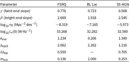
Table A1 Long description
The table presents best-fit parameters of the AGN evolutionary RLF for three types of AGN: FSRQ, BL Lac, and SS-AGN. It has four rows and eight columns. The columns are labeled with parameter names and their units or descriptions. The row labels are FSRQ, BL Lac, and SS-AGN. The parameters include gamma (faint-end slope), beta (bright-end slope), log base 10 of n0 (Mpc^-3 dex^-1), log base 10 of L-star(0) (W Hz^-1), kevo, ztop,0, deltatop, and mevo. The values for each parameter are listed row-wise for the three types of AGN. For example, the gamma values are 0.776 for FSRQ, 0.723 for BL Lac, and 0.508 for SS-AGN. The beta values are 2.669 for FSRQ, 1.918 for BL Lac, and 2.545 for SS-AGN. The table provides a detailed comparison of these parameters across different types of AGN.
A.3. HERG/LERG host probabilities and effective bias
Steep-spectrum AGN are split into excitation classes using stellar-mass scalings from Janssen et al. (Reference Janssen, Röttgering, Best and Brinchmann2012),
 \begin{align} P_\mathrm{LERG}(M_\star|z) &\propto \left(\frac{M_\star}{M_0}\right)^{2.5} \quad M_\star\lesssim10^{11.6}\,{\rm M}_\odot, \\[-25pt] \nonumber \end{align}
 \begin{align} P_\mathrm{HERG}(M_\star|z) &\propto \left(\frac{M_\star}{M_0}\right)^{1.5}, \end{align}
renormalised over candidate hosts. Mapping $M_\star$
to halo mass M via the stellar–halo relation (next subsection) yields the class-effective linear bias
$M_\star$
to halo mass M via the stellar–halo relation (next subsection) yields the class-effective linear bias
 \begin{align} b_t(z)\;=\;\frac{\displaystyle\int dM\, n(M,z)\,b(M,z)\,W_t(M,z)} {\displaystyle\int dM\, n(M,z)\,W_t(M,z)}\,, \qquad \\[-28pt] \nonumber \end{align}
 \begin{align} W_t\equiv P_t(M_\star(M,z),z), \\[6pt] \nonumber \end{align}
with n(M, z) the halo mass function and b(M, z) a standard halo-bias model. Since HERG-like weights favour higher $M_\star$
, Equation (A14) explains the robust bias hierarchy relative to SFG.
$M_\star$
, Equation (A14) explains the robust bias hierarchy relative to SFG.
A.4. Sizes
Our catalogue attaches a minimalist morphology proxy to each radio AGN solely to split the SSAGN pool into HERG/LERG-like sub-classes and apply class-dependent, stellar-mass-weighted halo assignment. Sizes do not affect photometry or clustering beyond the sub-class/host selection described here.
Following the approach of Bonaldi et al. (Reference Bonaldi, Bonato, Galluzzi, Harrison, Massardi, Kay, De Zotti and Brown2019), each AGN is given a characteristic linear size D (kpc) via a stochastic draw from the broad, observationally motivated distribution of DiPompeo et al. (Reference DiPompeo, Runnoe, Myers and Boroson2013) with a weak luminosity trend. A random sky orientation is applied (uniform in $\sin\theta$
). We do not simulate shapes or images; D is a single scale per source used only as a morphology proxy.
$\sin\theta$
). We do not simulate shapes or images; D is a single scale per source used only as a morphology proxy.
We compute a size-ratio
 \begin{equation} R_s \equiv \frac{d_\mathrm{peak}}{D_\mathrm{tot}},\end{equation}
the separation of the two peak-brightness regions $d_\mathrm{peak}$
divided by the end-to-end extent
$d_\mathrm{peak}$
divided by the end-to-end extent $D_\mathrm{tot}$
. We adopt the usual FR cut
$D_\mathrm{tot}$
. We adopt the usual FR cut $R_s\gt0.5 \Rightarrow$
FR II and
$R_s\gt0.5 \Rightarrow$
FR II and $R_s\lt0.5 \Rightarrow$
FR I. The draw of
$R_s\lt0.5 \Rightarrow$
FR I. The draw of $R_s$
is mildly luminosity-dependent: for
$R_s$
is mildly luminosity-dependent: for $L_\nu\le 10^{25.4}\,\mathrm{W\,Hz^{-1}}$
we take
$L_\nu\le 10^{25.4}\,\mathrm{W\,Hz^{-1}}$
we take $R_s\sim\mathcal{N}(\mu=0.18,\sigma=0.11)$
, and for
$R_s\sim\mathcal{N}(\mu=0.18,\sigma=0.11)$
, and for $L_\nu\gt10^{25.4}\,\mathrm{W\,Hz^{-1}}$
we take
$L_\nu\gt10^{25.4}\,\mathrm{W\,Hz^{-1}}$
we take $R_s\sim\mathcal{N}(\mu=0.62,\sigma=0.18)$
. This biases high-power sources towards FR II while still allowing overlap in
$R_s\sim\mathcal{N}(\mu=0.62,\sigma=0.18)$
. This biases high-power sources towards FR II while still allowing overlap in $R_s$
at fixed L.
$R_s$
at fixed L.
We then assign the spectroscopic class with a deterministic rule at fixed $R_s$
: sources with
$R_s$
: sources with $R_s\gt0.5$
are tagged as HERG, and those with
$R_s\gt0.5$
are tagged as HERG, and those with $R_s\le 0.5$
as LERG. Because
$R_s\le 0.5$
as LERG. Because $R_s$
itself is drawn with scatter, the resulting fractions vary smoothly with luminosity; in particular
$R_s$
itself is drawn with scatter, the resulting fractions vary smoothly with luminosity; in particular
 \begin{equation}P(\mathrm{HERG}\,|\,L)= P(R_s\gt0.5\,|\,L)= 1 - \Phi\!\left(\frac{0.5-\mu(L)}{\sigma(L)}\right),\end{equation}
with $\Phi$
the standard normal CDF and
$\Phi$
the standard normal CDF and $(\mu(L),\sigma(L))$
given above. Hence FR II–LERG and FR I–HERG combinations naturally occur, even though the label is a hard threshold in
$(\mu(L),\sigma(L))$
given above. Hence FR II–LERG and FR I–HERG combinations naturally occur, even though the label is a hard threshold in $R_s$
.
$R_s$
.
A.5. Stellar–halo mass relation (for host selection)
Host selection uses a redshift-dependent double-power relation (Bonaldi et al. Reference Bonaldi, Bonato, Galluzzi, Harrison, Massardi, Kay, De Zotti and Brown2019; Aversa et al. Reference Aversa, Lapi, de Zotti, Shankar and Danese2015),
 \begin{equation}M_\star(M,z) \;=\; N_0(z)\,\left[\left(\frac{M}{M_b(z)}\right)^{\epsilon(z)}+ \left(\frac{M}{M_b(z)}\right)^{\omega(z)}\right]^{-1},\end{equation}
interpolated from the fit of Aversa et al. (Reference Aversa, Lapi, de Zotti, Shankar and Danese2015). This sets AGN host probabilities (via $M_\star$
) and provides the smooth proxy used to fit the SFG L(M) map. Steepening at high mass boosts HERG bias relative to LERG; shifts in
$M_\star$
) and provides the smooth proxy used to fit the SFG L(M) map. Steepening at high mass boosts HERG bias relative to LERG; shifts in $M_b(z)$
move the characteristic host mass and reshape class-specific n(z) tails.
$M_b(z)$
move the characteristic host mass and reshape class-specific n(z) tails.
A.6. SFG radio luminosities: Synchrotron and free–free
We model the SFG spectrum as a sum of non-thermal synchrotron and thermal free–free components (Bonaldi et al. Reference Bonaldi, Bonato, Galluzzi, Harrison, Massardi, Kay, De Zotti and Brown2019; Mancuso et al. Reference Mancuso2015). The synchrotron component is
 \begin{equation}L_\mathrm{sync}(\nu) \;=\;\frac{L_{*,\mathrm{sync}}(\nu)} {\left(\dfrac{L_{*,\mathrm{sync}}}{\bar{L}_\mathrm{sync}}\right)^{\beta} + \left(\dfrac{L_{*,\mathrm{sync}}}{\bar{L}_\mathrm{sync}}\right)} ,\end{equation}
with fiducial scaling
 \begin{align}\begin{split}\bar{L}_\mathrm{sync} \;=\; 1.9\times10^{21}\left( \frac{\mathrm{SFR}}{M_\odot\,\mathrm{yr}^{-1}} \right)\left( \frac{\nu}{\mathrm{GHz}} \right)^{-0.85}\\[3pt]{\left[ 1 + \left( \frac{\nu}{20\,\mathrm{GHz}} \right)^{0.5} \right]}^{-1}\;\mathrm{W\,Hz^{-1}}\!.\end{split}\end{align}
The free–free component follows
 \begin{equation}L_\mathrm{ff}(\nu) \;\propto\; T^{-0.5}\, g_\mathrm{ff}(\nu,T)\,\nu^{-0.1},\qquad T=10^4\,\mathrm{K},\end{equation}
with Gaunt factor (van Hoof et al. Reference van Hoof, Williams, Volk, Chatzikos, Ferland, Lykins, Porter and Wang2014)
 \begin{equation}\begin{aligned}g_\mathrm{ff}(\nu_\mathrm{GHz},T)&= \ln \Bigl(e + \exp \Bigl[5.960 - \frac{\sqrt{3}}{\pi}\,\ln \bigl(\nu_\mathrm{GHz}\,T_4^{-3/2}\bigr)\Bigr]\Bigr),\\T_4 &\equiv T/10^4\,\mathrm{K}.\end{aligned}\end{equation}
Below $\sim$
10–20 GHz, synchrotron with
$\sim$
10–20 GHz, synchrotron with $\zeta\!\approx\!0.8$
–0.9 dominates; free–free adds a flatter
$\zeta\!\approx\!0.8$
–0.9 dominates; free–free adds a flatter $\zeta\!\approx\!0.1$
tail, making extrapolations to a few GHz slightly shallower than pure synchrotron. Together with a smoothly evolving SFG RLF, this SED reproduces multi-frequency counts.
$\zeta\!\approx\!0.1$
tail, making extrapolations to a few GHz slightly shallower than pure synchrotron. Together with a smoothly evolving SFG RLF, this SED reproduces multi-frequency counts.
A.7. Thermal dust normalisation and IR-calibrated cross-check
This subsection collects the working relations used for the thermal dust SED term and for the IR-calibrated SFG cross-check described in Section 3.2.1.
A.7.1. Dust normalisation
The thermal dust component is modelled as a greybody (Equation 2) and is normalised by the integrated infrared luminosity over 8–1 000 $\unicode{x03BC}$
m,
$\unicode{x03BC}$
m,
 \begin{equation}\int_{\nu(1\,000\,\unicode{x03BC}\mathrm{m})}^{\nu(8\,\unicode{x03BC}\mathrm{m})} L_\nu^\mathrm{dust}\,{d}\nu\equiv L_\mathrm{{IR}} .\end{equation}
We relate $L_\mathrm{{IR}}$
to SFR using the calibration adopted in T-RECS,
$L_\mathrm{{IR}}$
to SFR using the calibration adopted in T-RECS,
 \begin{equation}\log_{10}\!\left(\frac{L_\mathrm{{IR}}}{L_\odot}\right)=\log_{10}\!\left(\frac{\mathrm{SFR}}{M_\odot\,\mathrm{yr}^{-1}}\right)+ 9.892 ,\end{equation}
so that the greybody normalisation $A_{d}$
is uniquely specified for given
$A_{d}$
is uniquely specified for given $(T_{d},\beta_{d})$
.
$(T_{d},\beta_{d})$
.
A.7.2. IR-radio mapping for the cross-check
An IR-calibrated estimate of the SFG radio space density is obtained by mapping an IR luminosity function $\Phi_\mathrm{{IR}}(L_\mathrm{{IR}},z)$
to an effective 1.4 GHz luminosity function using the IR-radio correlation parameter q (Yun et al. Reference Yun, Reddy and Condon2001),
$\Phi_\mathrm{{IR}}(L_\mathrm{{IR}},z)$
to an effective 1.4 GHz luminosity function using the IR-radio correlation parameter q (Yun et al. Reference Yun, Reddy and Condon2001),
 \begin{align}q\equiv\log_{10}\!\left(\frac{L_\mathrm{{IR}}/(3.75\times 10^{12}\,\mathrm{W})}{L_{1.4}}\right),\qquad q \sim \mathcal{N}(q_0,\sigma_q^2),\end{align}
which implies
 \begin{equation}\log_{10} L_{1.4}=\log_{10} L_\mathrm{{IR}}-\log_{10}\!(3.75\times10^{12}\,\mathrm{W})-q .\end{equation}
The corresponding $\Phi_{1.4}(L_{1.4},z)$
follows by change of variables and convolution over P(q). For
$\Phi_{1.4}(L_{1.4},z)$
follows by change of variables and convolution over P(q). For $\Phi_\mathrm{{IR}}$
, a Saunders-form parameterisation for late-type and starburst galaxies and its redshift evolution is adopted following Cai et al. (Reference Cai2013). This construction is used only as a sensitivity test (Section 5.10).
$\Phi_\mathrm{{IR}}$
, a Saunders-form parameterisation for late-type and starburst galaxies and its redshift evolution is adopted following Cai et al. (Reference Cai2013). This construction is used only as a sensitivity test (Section 5.10).
A.8. Abundance matching and the working L(M) map
We assign radio luminosities to halos monotonically in each redshift slice so the realised luminosity histogram reproduces the target RLF. For SFG we fit
 \begin{equation}L(M;\,z) \;=\; N(z)\,\left[\left(\frac{M}{M_\star(z)}\right)^{\gamma}+ \left(\frac{M}{M_\star(z)}\right)^{\beta}\right]^{-1},\end{equation}
apply a log-normal scatter $\sigma_{\log L}$
, and perform rank-ordering without replacement. Parameters are inferred per slice with a Poisson likelihood for the RLF-implied counts. Equation (A26) behaves as a flexible double-slope map:
$\sigma_{\log L}$
, and perform rank-ordering without replacement. Parameters are inferred per slice with a Poisson likelihood for the RLF-implied counts. Equation (A26) behaves as a flexible double-slope map: $\gamma$
controls the faint-end response to host mass,
$\gamma$
controls the faint-end response to host mass, $\beta$
the bright-end roll-off,
$\beta$
the bright-end roll-off, $M_\star$
the transition scale, and N the normalisation; the scatter compresses the effective L–M relation and slightly lowers bias at fixed L. For AGN, we first draw hosts with the mass-weighted HERG/LERG probabilities and then assign L monotonically within the selected subset to match the class RLFs, keeping bias tied to halo mass (Equation A14).
$M_\star$
the transition scale, and N the normalisation; the scatter compresses the effective L–M relation and slightly lowers bias at fixed L. For AGN, we first draw hosts with the mass-weighted HERG/LERG probabilities and then assign L monotonically within the selected subset to match the class RLFs, keeping bias tied to halo mass (Equation A14).
A.9. From populations to observables: Effective kernels and bias
Given the above ingredients, the selection-matched redshift kernel for class X is
 \begin{align}\begin{split}\varphi_X(z)=\frac{n_X(z)}{\int n_X(z')\,dz'}\,,\qquad\\[2pt] \text{where } n_X(z)\text{ is given by Equation (A5)}.\end{split}\end{align}
For the auto-correlation of tracer X, the effective large-scale bias entering $C_\ell$
or
$C_\ell$
or $w(\theta)$
is
$w(\theta)$
is
 \begin{equation}b_{\mathrm{eff},X}=\left[\frac{\displaystyle \int dz\,\varphi_X^2(z)\,b_X^2(z)\,D^2(z)} {\displaystyle \int dz\,\varphi_X^2(z)\,D^2(z)}\right]^{1/2}.\end{equation}
with D(z) the growth factor, that is, $\delta_m(k,z)=D(z)\delta_m(k,z=0)$
, and
$\delta_m(k,z)=D(z)\delta_m(k,z=0)$
, and $b_X(z)$
from Equation (A14). Changes to the survey selection alter
$b_X(z)$
from Equation (A14). Changes to the survey selection alter $\varphi_X(z)$
(projection) and therefore the amplitude/slope of
$\varphi_X(z)$
(projection) and therefore the amplitude/slope of $w(\theta)$
without changing the intrinsic bias ordering set by
$w(\theta)$
without changing the intrinsic bias ordering set by $b_X(z)$
.
$b_X(z)$
.
A.10. SFR function
We use the SFR density function (constrained by observations) from (Bonaldi et al. Reference Bonaldi, Bonato, Galluzzi, Harrison, Massardi, Kay, De Zotti and Brown2019; Mancuso et al. Reference Mancuso2015)
 \begin{align}\begin{split}\phi_{\mathrm{SFR}}(z) \;=\; \Phi(z)\,\left[ \frac{\mathrm{SFR}}{\mathrm{SFR}_*(z)} \right]^{1 - \zeta(z)}\\[3pt]\exp \!\left\{- \left[ \frac{\mathrm{SFR}}{\mathrm{SFR}_*(z)} \right]^{w(z)} \right\},\end{split} \end{align}
with redshift evolution
 \begin{align}\log \Phi(z)\,[\mathrm{Mpc}^{-3}\log(\mathrm{SFR})^{-1}]&= -2.4 - 2.3\chi \nonumber\\[2pt]&\quad {}+ 6.2\chi^2 - 4.9\chi^3, \end{align}
 \begin{align}\log \mathrm{SFR}_*(z)\,[M_\odot\,\mathrm{yr}^{-1}]&= 1.1 + 3.2\chi \nonumber\\[2pt]&\quad {}- 1.4\chi^2 - 2.1\chi^3, \end{align}
 \begin{align}\zeta(z)&= 1.2 + 0.5\chi {}- 0.5\chi^2 + 0.2\chi^3, \end{align}
 \begin{align}w(z)&= 0.7 - 0.15\chi {}+ 0.16\chi^2 + 0.01\chi^3.\end{align}
where $\chi=\log(1+z)$
. In GHOST the SFG branch is radio-first; this SFRF is kept as an optional cross-check to sanity-test the bright tail of
$\chi=\log(1+z)$
. In GHOST the SFG branch is radio-first; this SFRF is kept as an optional cross-check to sanity-test the bright tail of $\Phi_\mathrm{{SFG}}$
at
$\Phi_\mathrm{{SFG}}$
at $z\gtrsim1$
without imposing IR-radio priors.
$z\gtrsim1$
without imposing IR-radio priors.


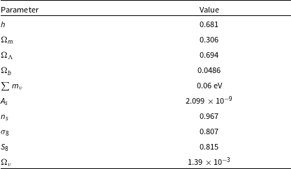
 Λ
Λ z=0
z=0 Ωm
Ωm ΩΛ
ΩΛ Ωb
Ωb ∑mν
∑mν As
As ns
ns 8h−1Mpc
 σ8
σ8 S8≡σ8Ωm/0.3
 Ων
Ων Ωνh2=∑mν/(93.14eV)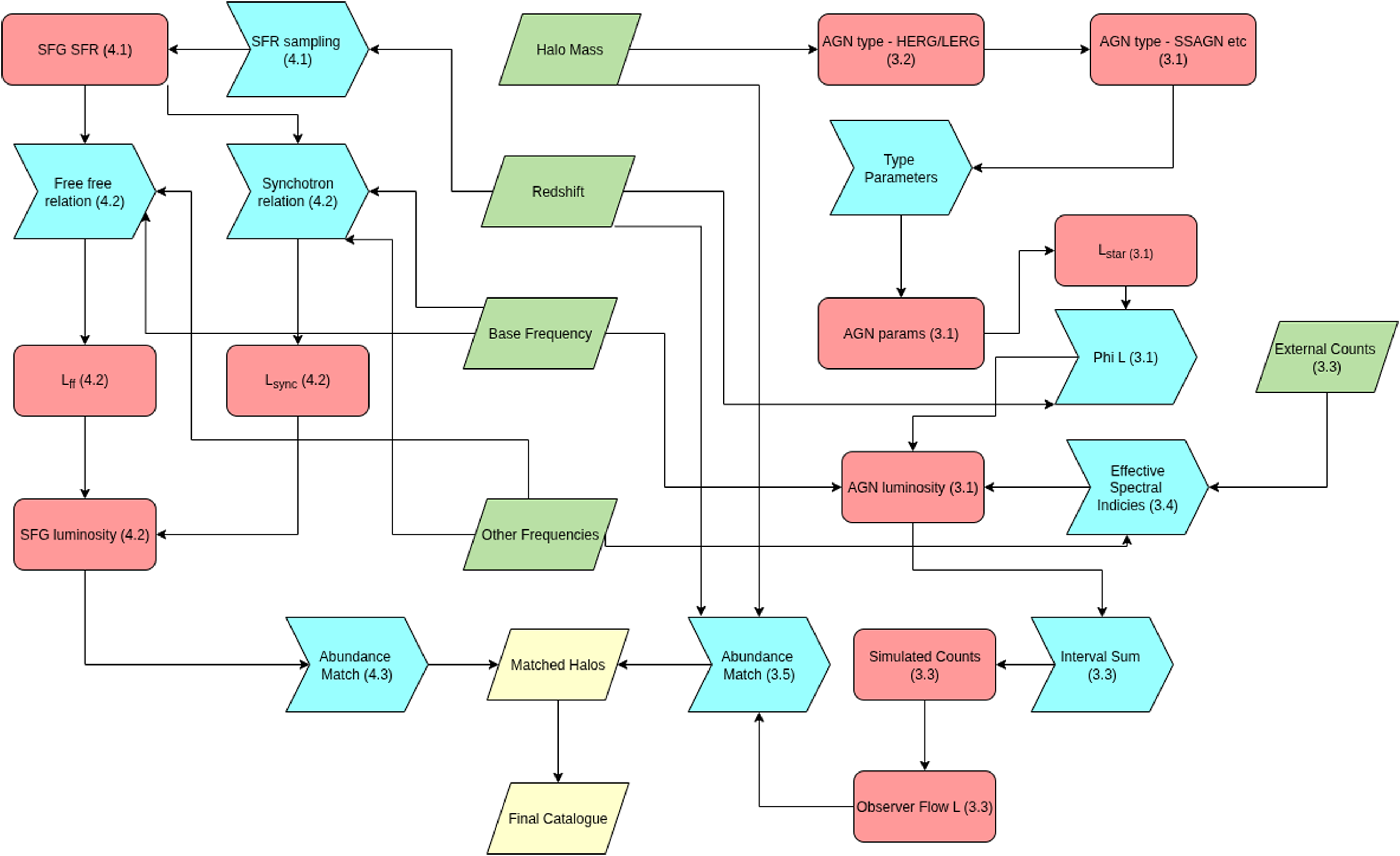
 Φ(L)
Φ(L) Lff
Lff Lsync
Lsync L⋆
L⋆ Φ(L)
Φ(L)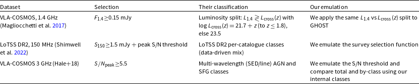
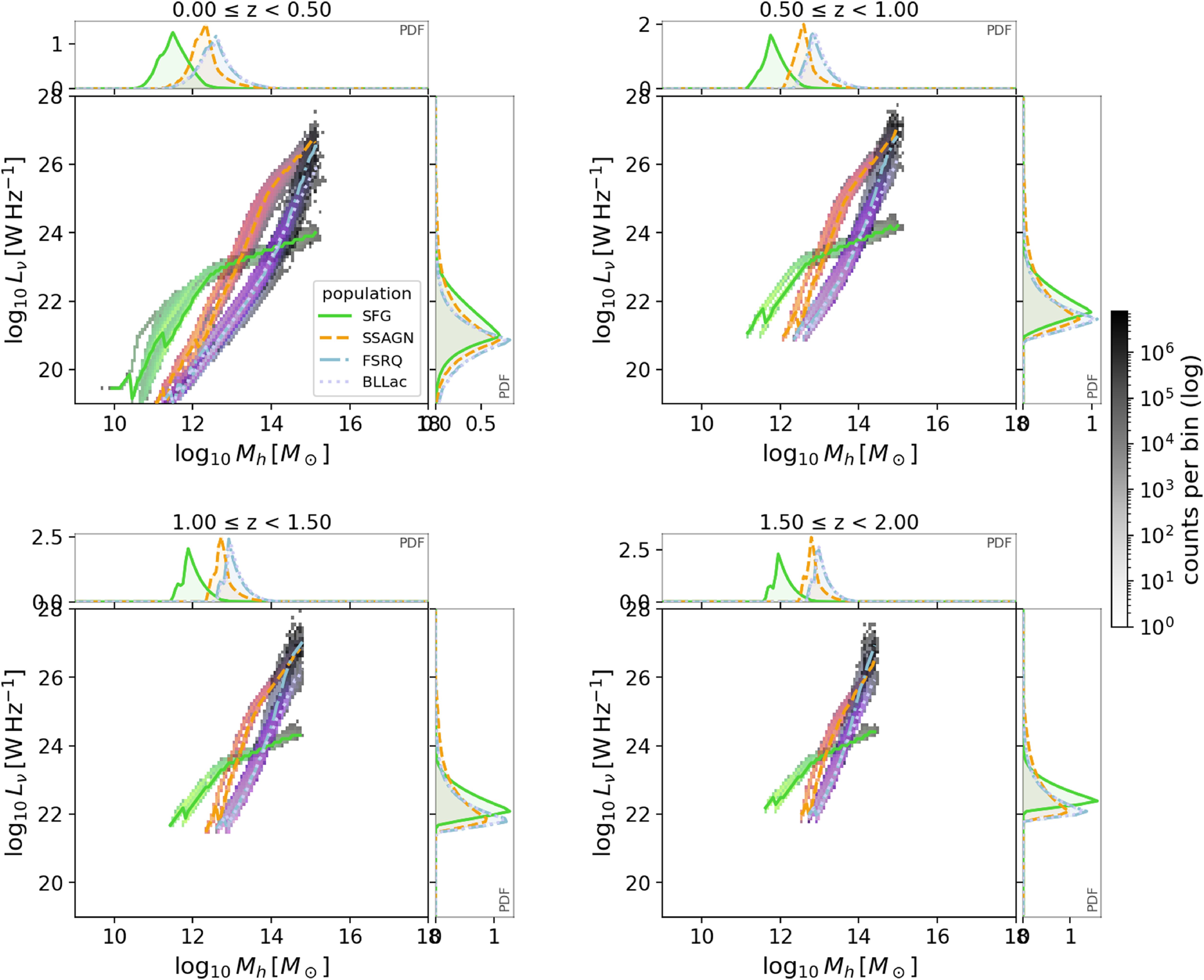
 log10Lν
 log10Mh
 p(log10Mh)
 p(log10Lν)
 ∫pdlogMh=1
 ∫pdlogL=1
 Mh
Mh Lν
Lν Mh
Mh Mh
Mh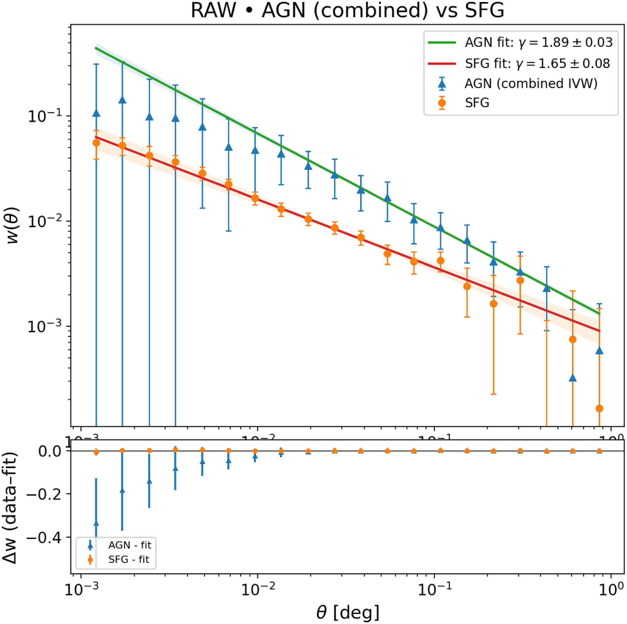
 w(θ)
w(θ) w(θ)=A(θ/θ0)1−γ
 θ∈[0.02∘,1.0∘]
 1σ
1σ (A,γ)
(A,γ) γAGN=1.886±0.028
 γSFG=1.647±0.076
 −
− >
> ϕ(z)
ϕ(z) k=ℓ/χ(z)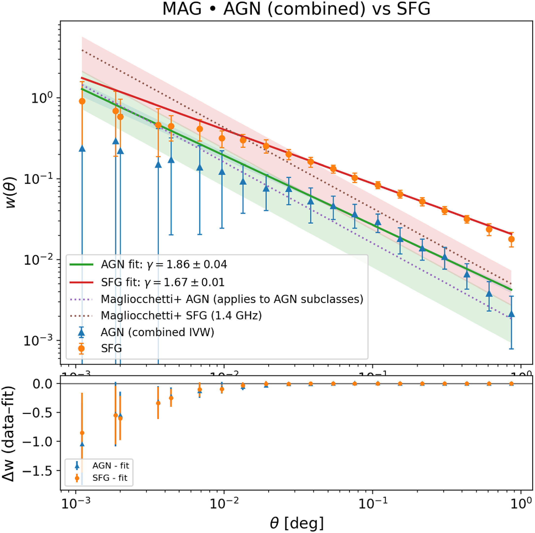
 w(θ)
w(θ) L1.4≷Lcross(z)
 θ∈[0.02∘,1.0∘]
 1σ
1σ γAGN=1.858±0.041
 γSFG=1.667±0.010
 zeff≃0.094
 χeff≃0.41
 θ
θ r⊥
r⊥ r⊥(0.05∘)≈0.35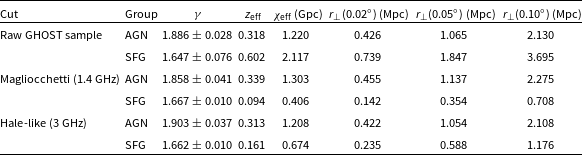
 1σ
1σ θ∈[0.02∘,0.5∘]
 r⊥(θ)=θχeff
 Cℓ
Cℓ ℓ∈[40,250]
 b=
b= b(z)=b0(1+z)ζ
 χ2
χ2 b/bSFG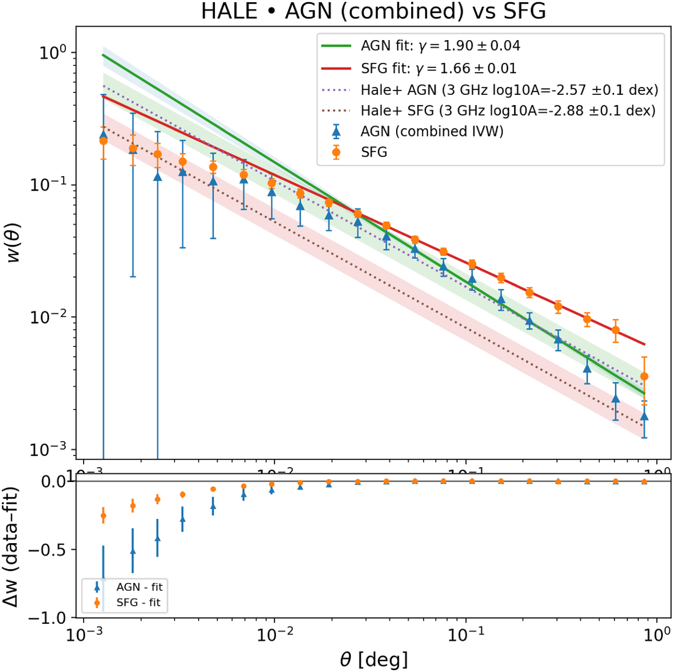
 γAGN=1.903±0.037
 γSFG=1.662±0.010
 zeff,SFG≃0.161
 χeff,SFG≃0.67
 r⊥(0.05∘)≈0.59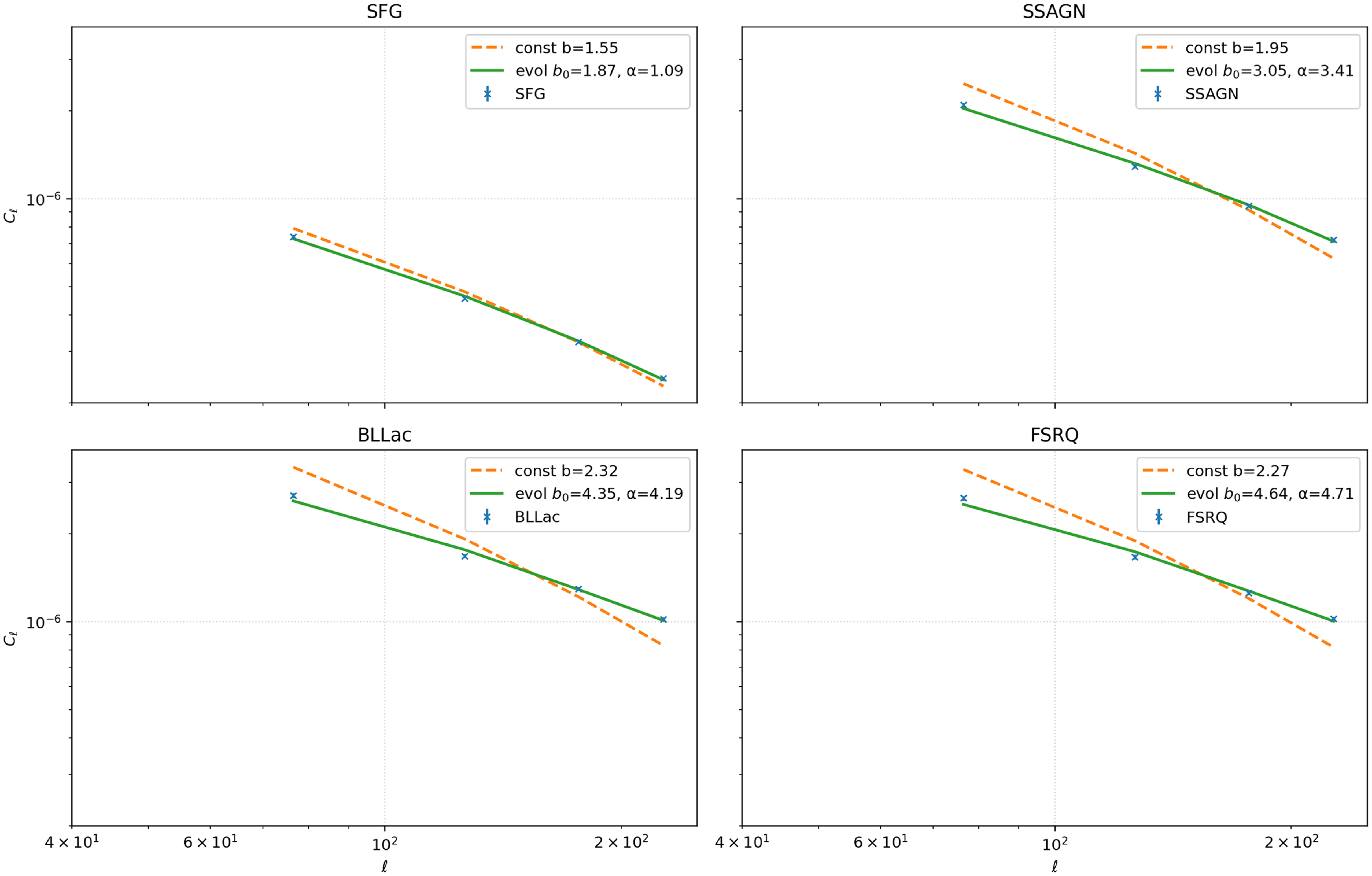
 Cℓ
Cℓ b=
b= b(z)=b0(1+z)ζ
 ℓ∈[40,250]
 <
< ≲
≲ ≃
≃ ζ
ζ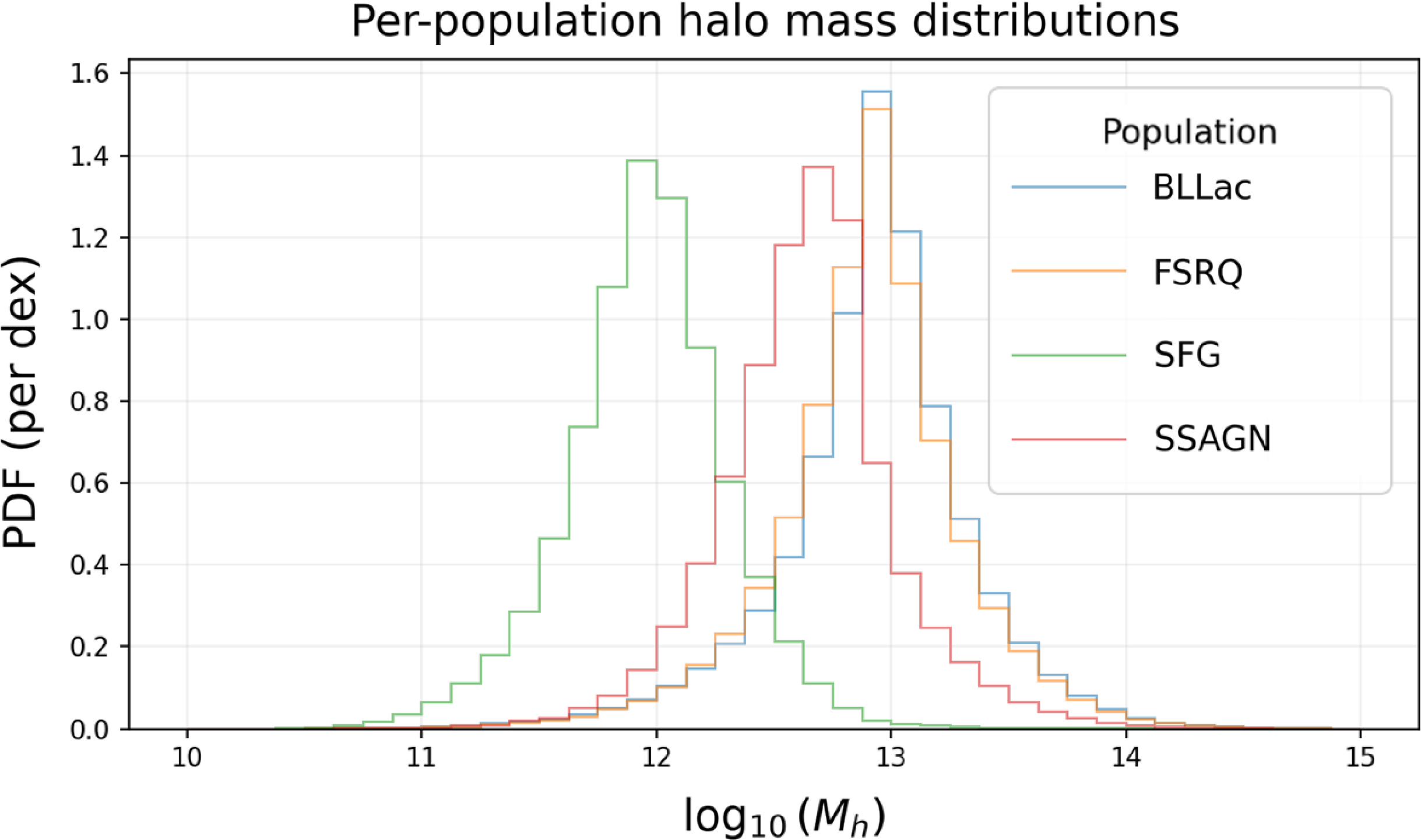
 log10(Mh/M⊙)
 1012.8−13
 ⊙
⊙ 1012
1012 ⊙
⊙
 med[log10Mh/M⊙]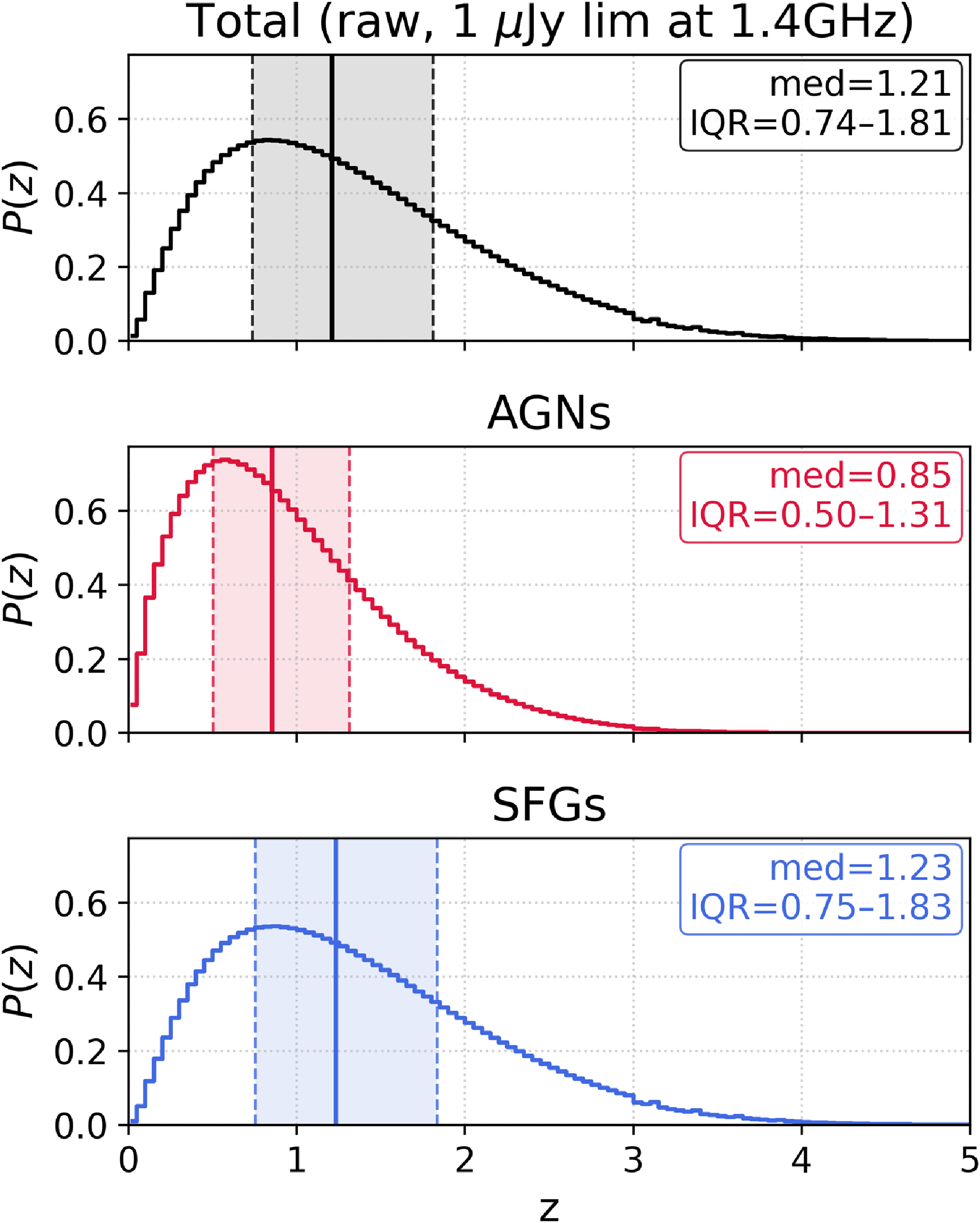
 z∼0.8
z∼0.8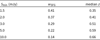
 wSFG
wSFG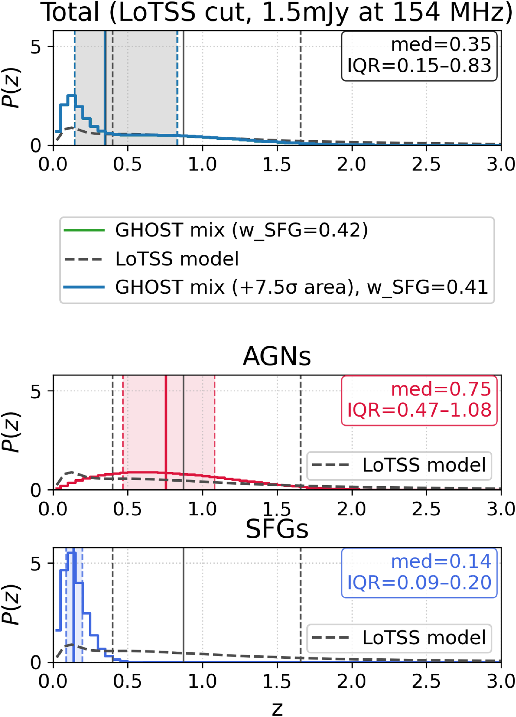
 S150≥1.5mJy
 wSFGPSFG(z)+wAGNPAGN(z)
 (wSFG,wAGN)
 PSFG(z),PAGN(z)
 ≥7.5
≥7.5 σ~=83μJybeam−1
 171μJybeam−1
 z≲0.4
z≲0.4 z≳0.6
z≳0.6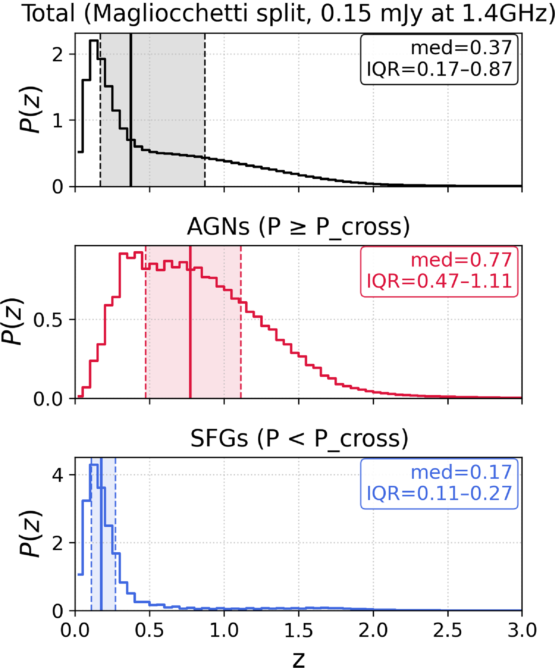
 F1.4≥0.15
 L1.4≷Lcross(z)
 Lcross=4πPcross
 log10Pcross(z)=21.7+z
 z≤1.8
z≤1.8 23.5
23.5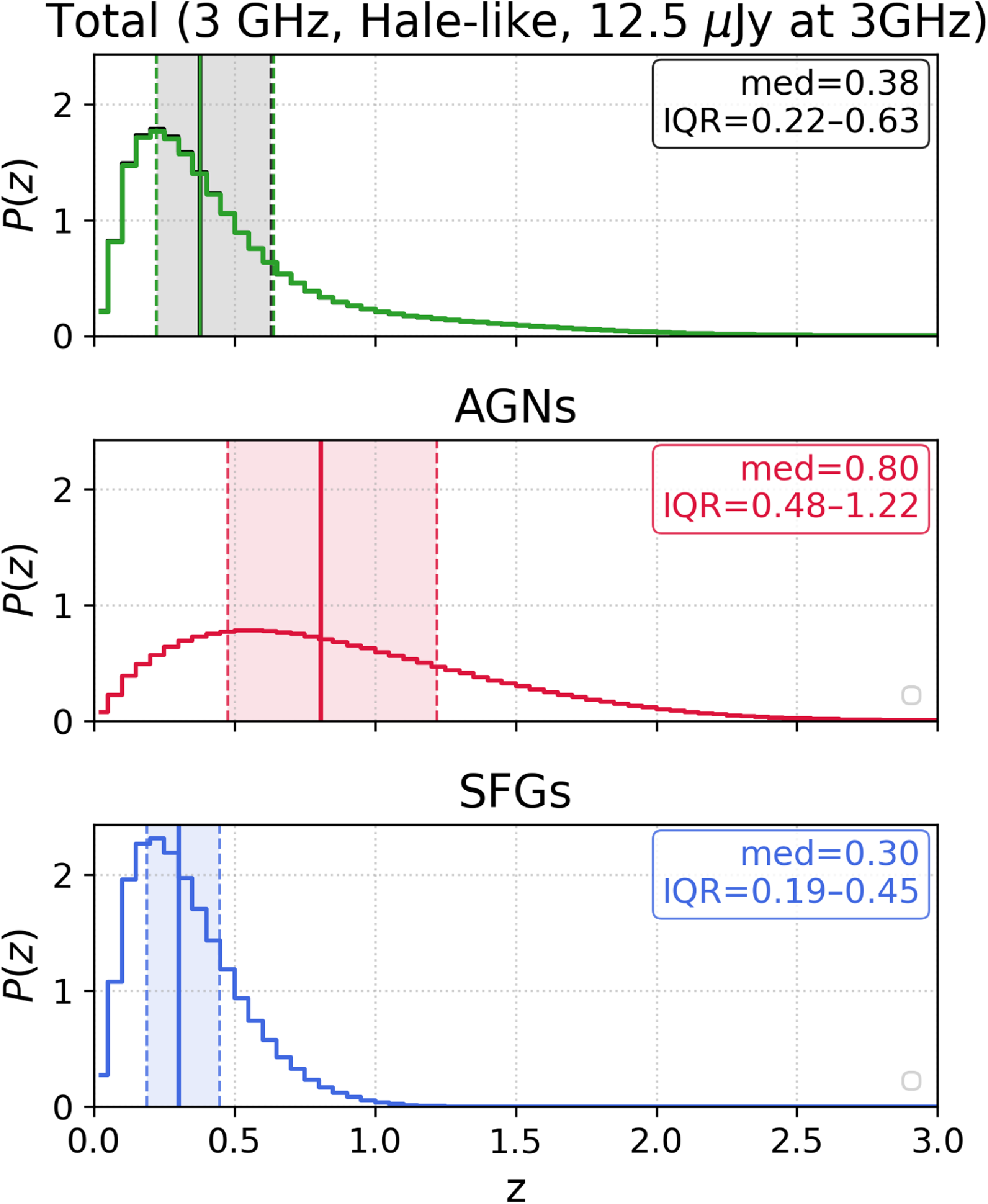
 S/N≥5.5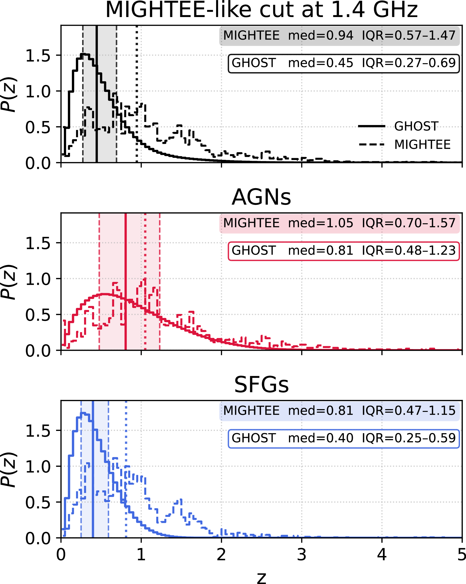
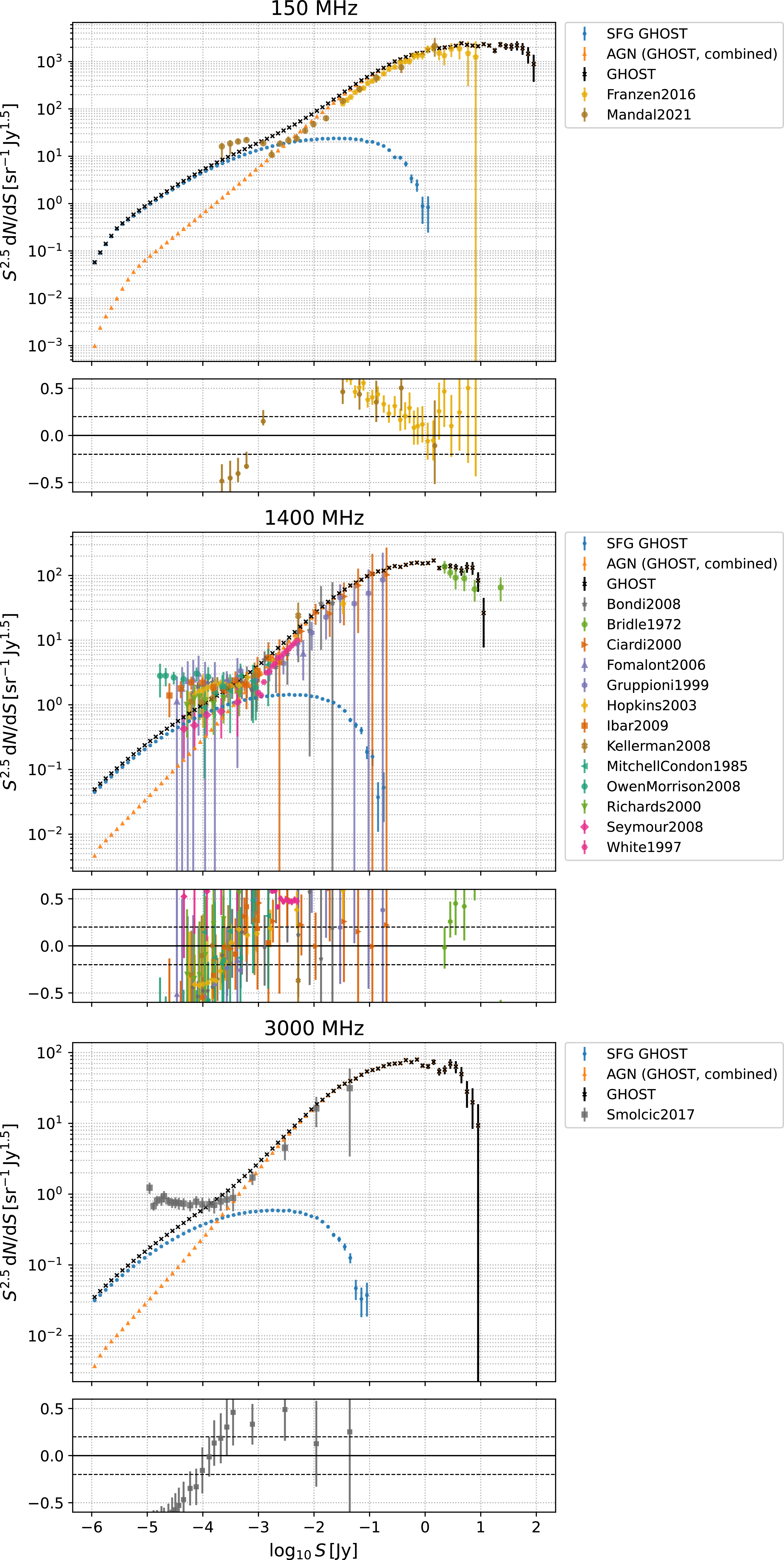
 S2.5dN/dS
 c˘
c˘ 1σ
1σ N<20
N<20 (model−data)/data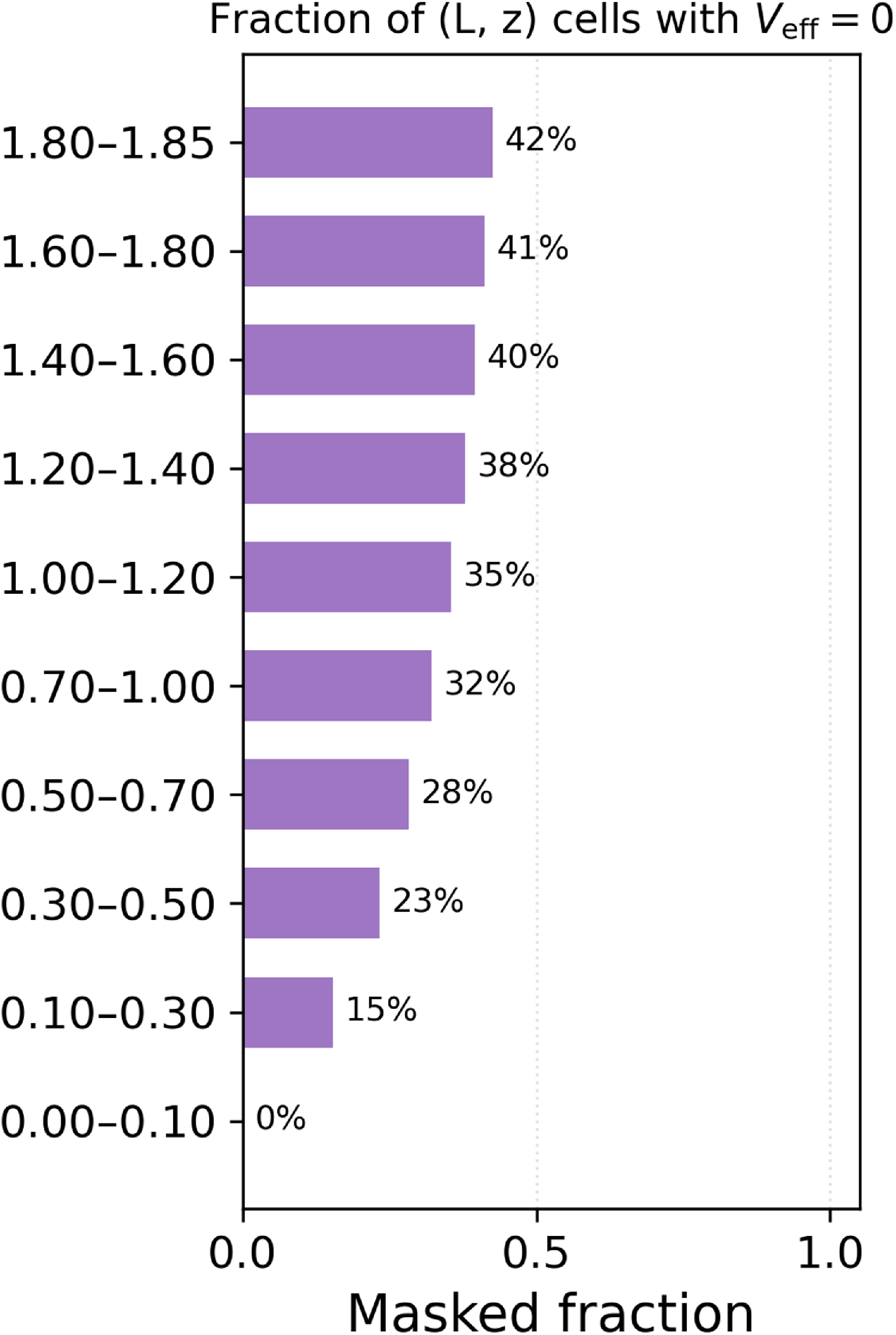
 Veff=0
 ≲
≲ 0.5%
0.5% ≲
≲ z≤0.3
z≤0.3 ≃
≃ z∼1.8
z∼1.8 Veff=0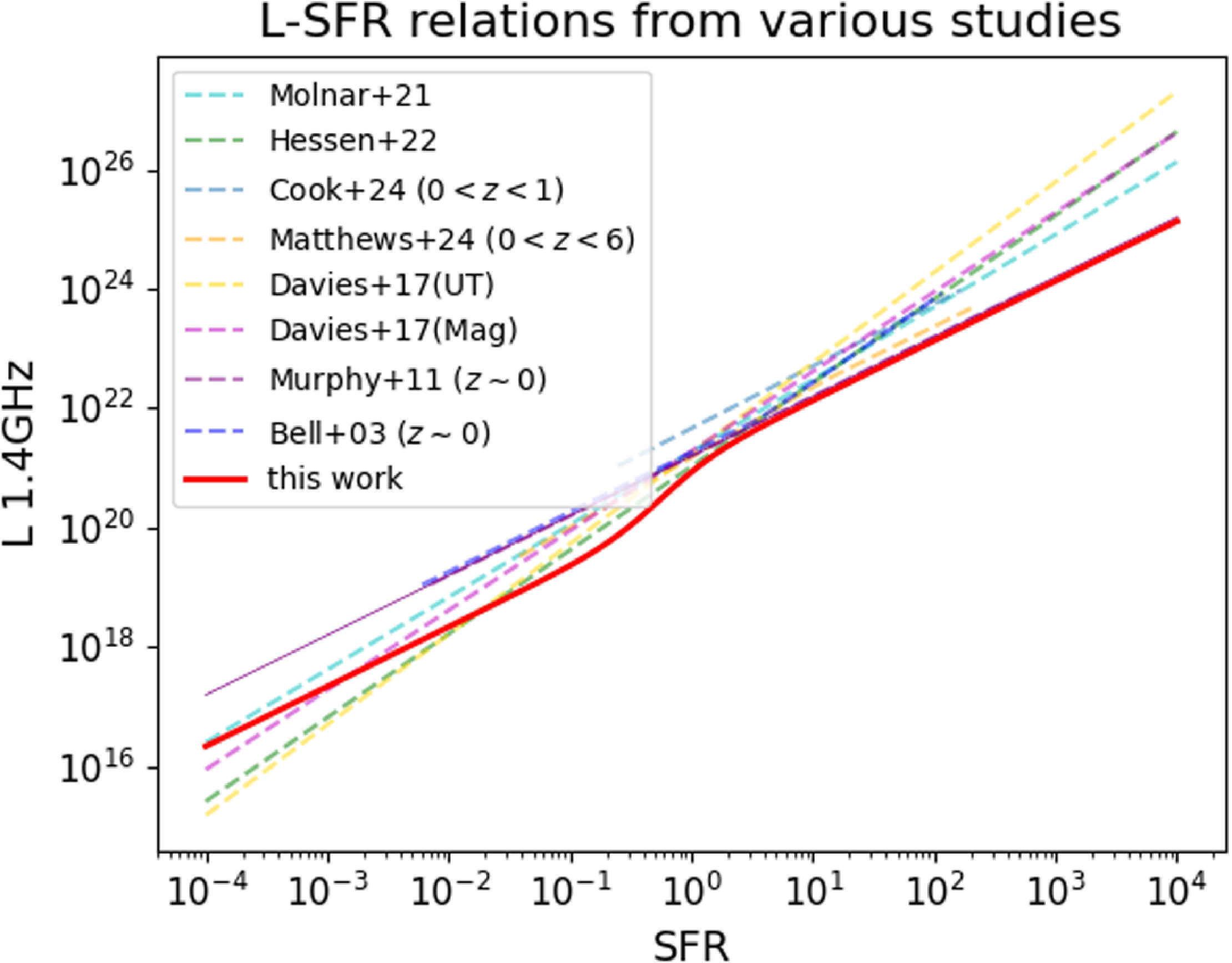
 ϕSFR(z)
 L1.4
L1.4 L1.4≳1023-24WHz−1
 z≳1
z≳1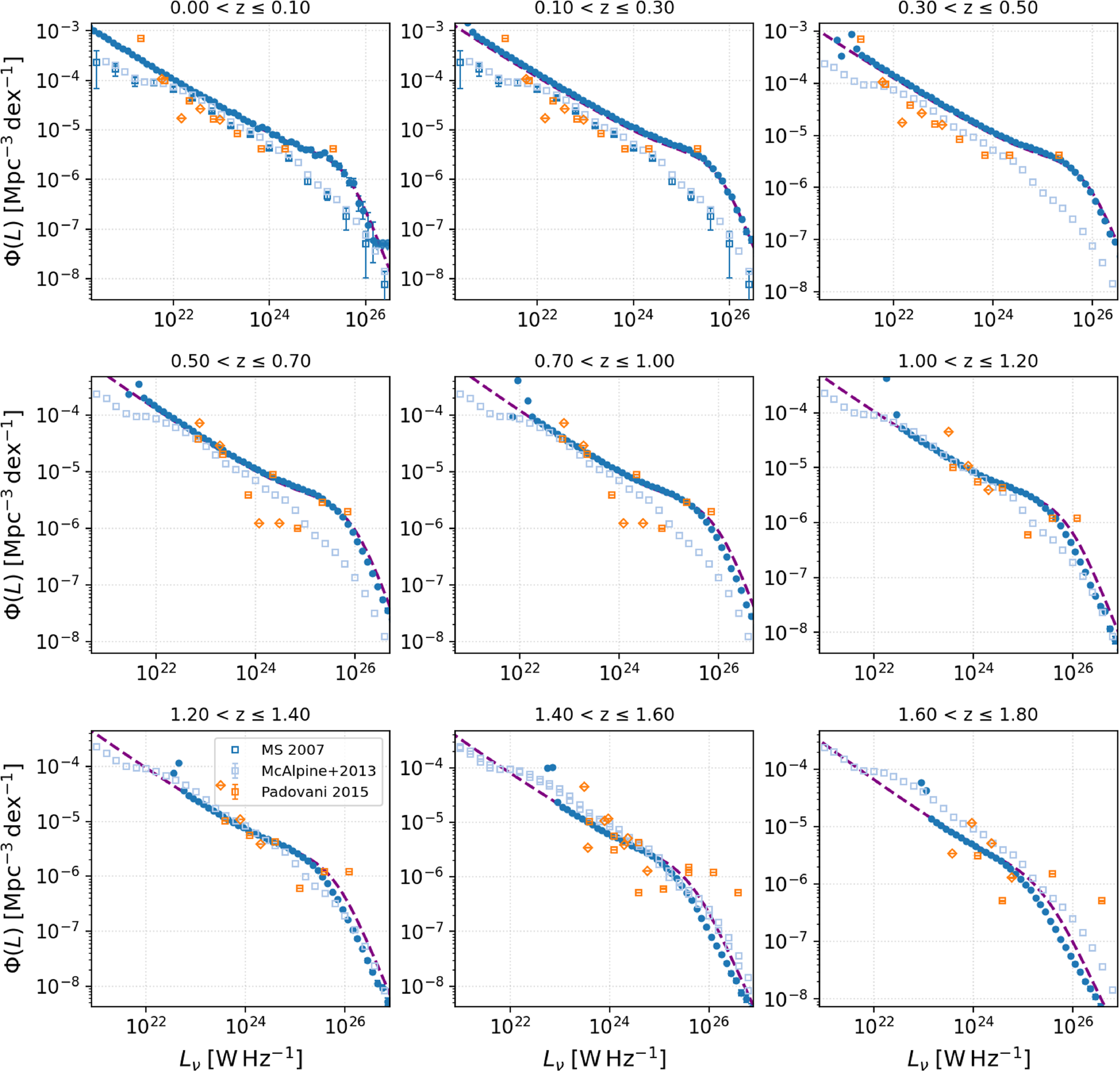
 Φ(Lν)(Mpc−3dex−1)
 Φ=N/(VeffΔlog10L)
 Veff
Veff 1σ
1σ Veff
Veff Veff=0
 Φproj(L|z1:z2)
 Δz
Δz Lν∼1026WHz−1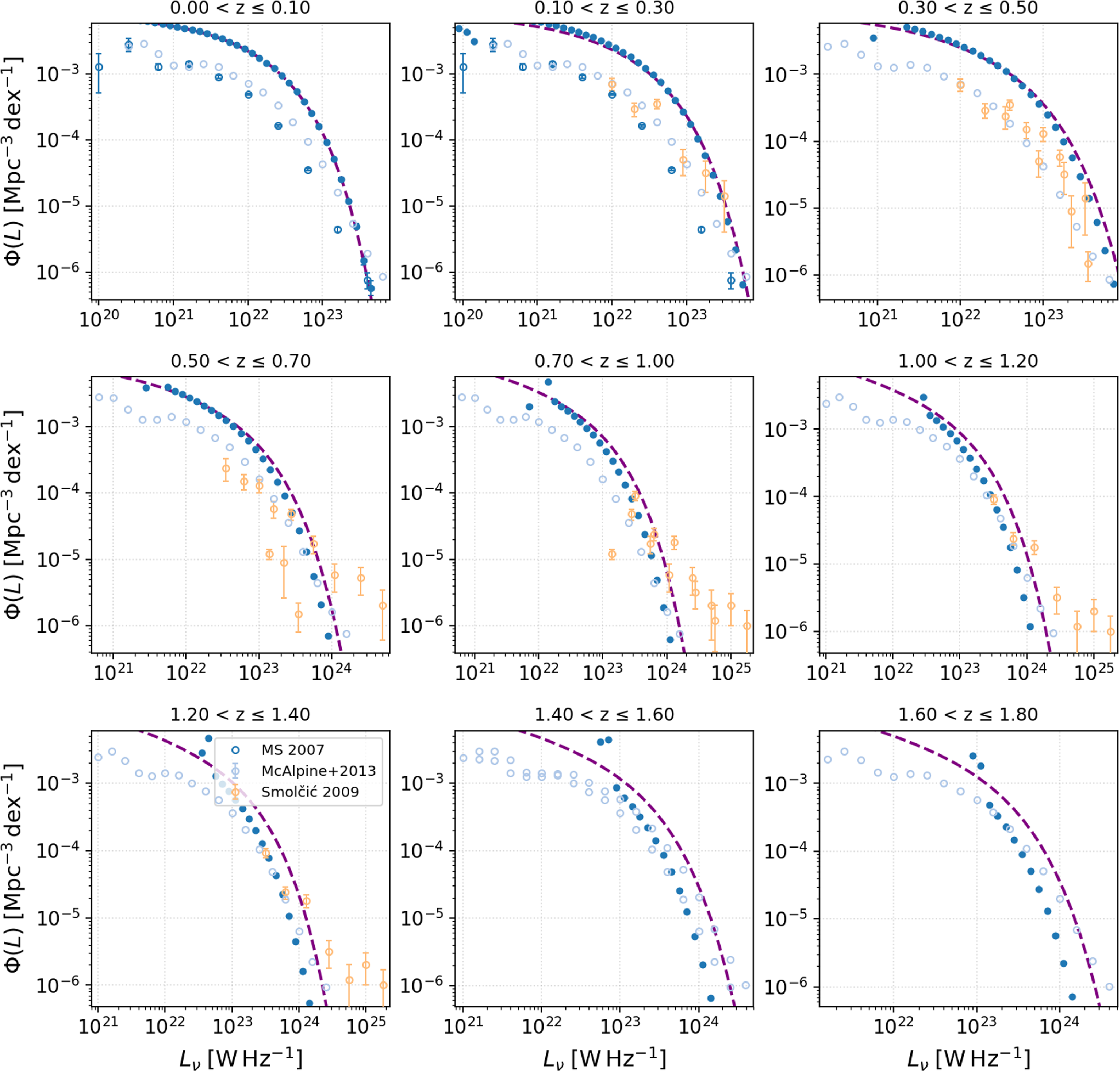
 Φ=N/(VeffΔlog10L)
 1σ
1σ Δz
Δz z≲1
z≲1 Δz
Δz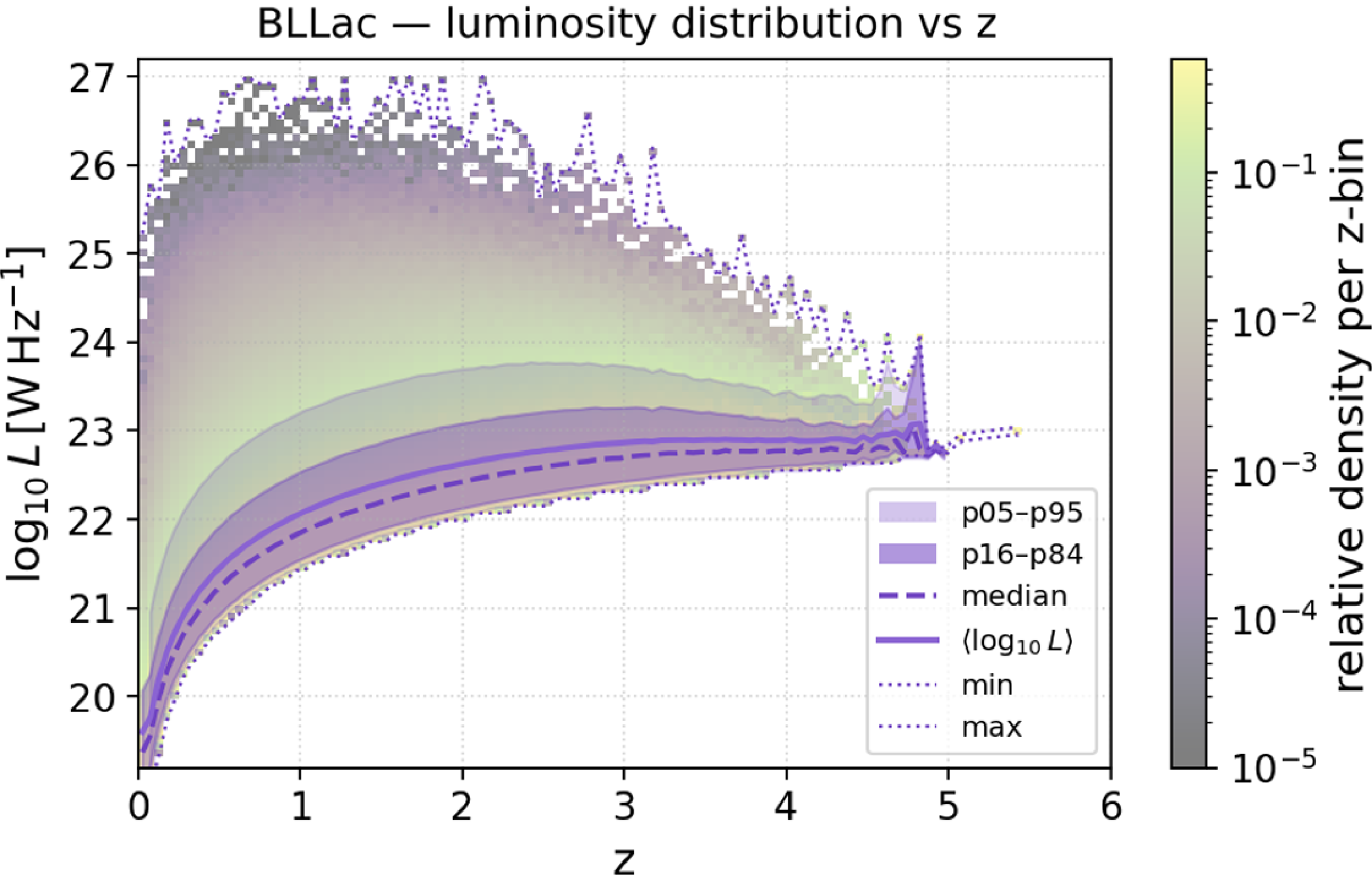
 log10Lν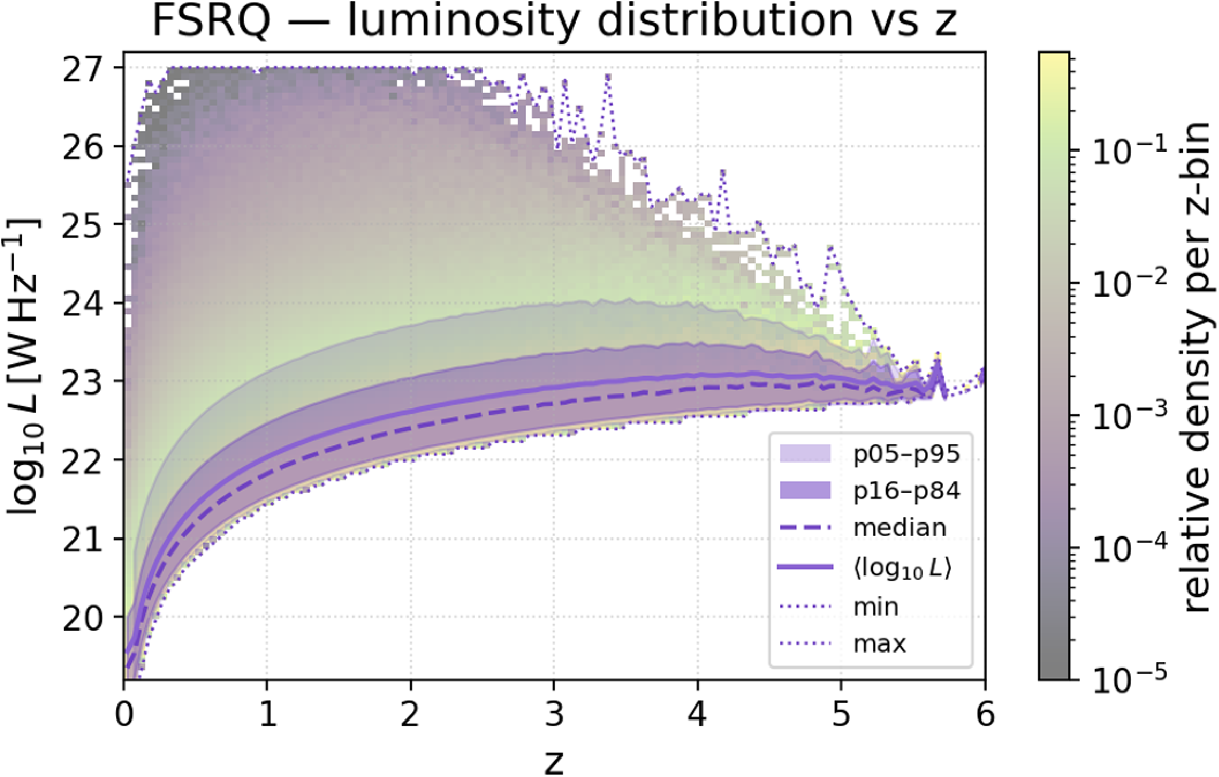
 z≲1
z≲1 z∼3
z∼3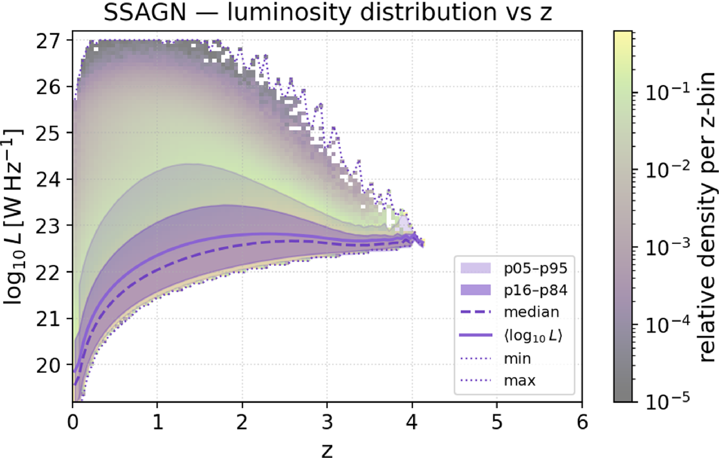
 z∼1
z∼1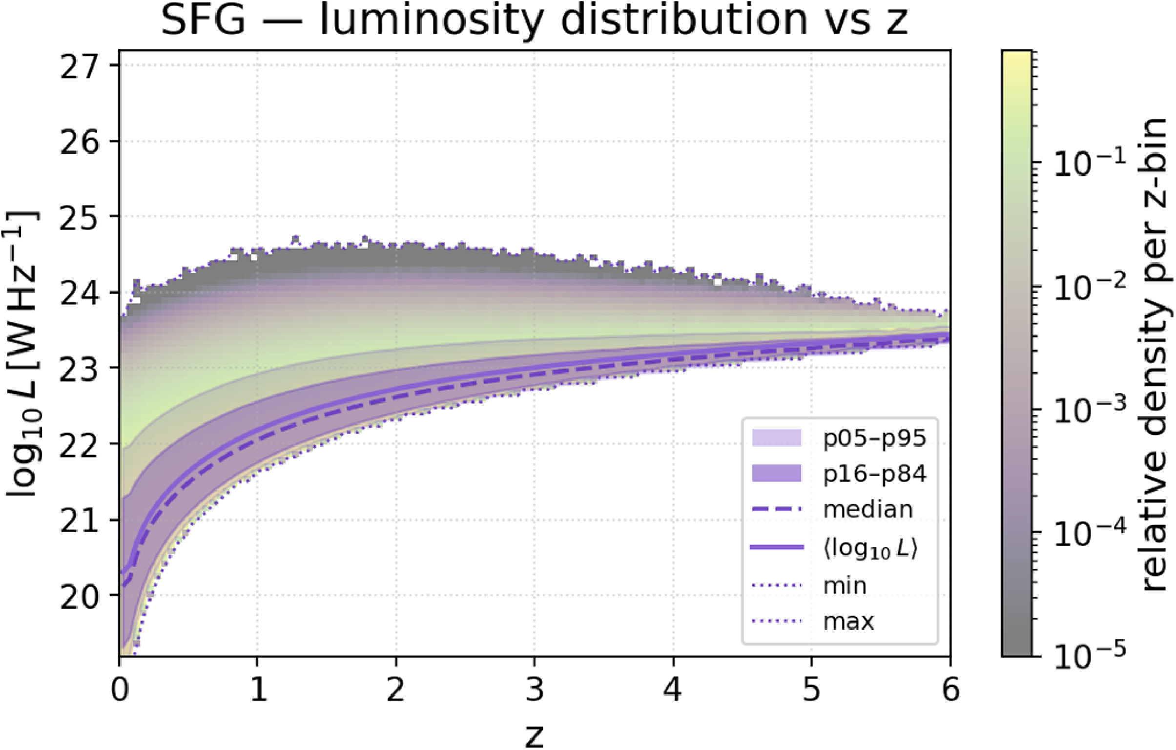
 z∼2
z∼2 z∼3
z∼3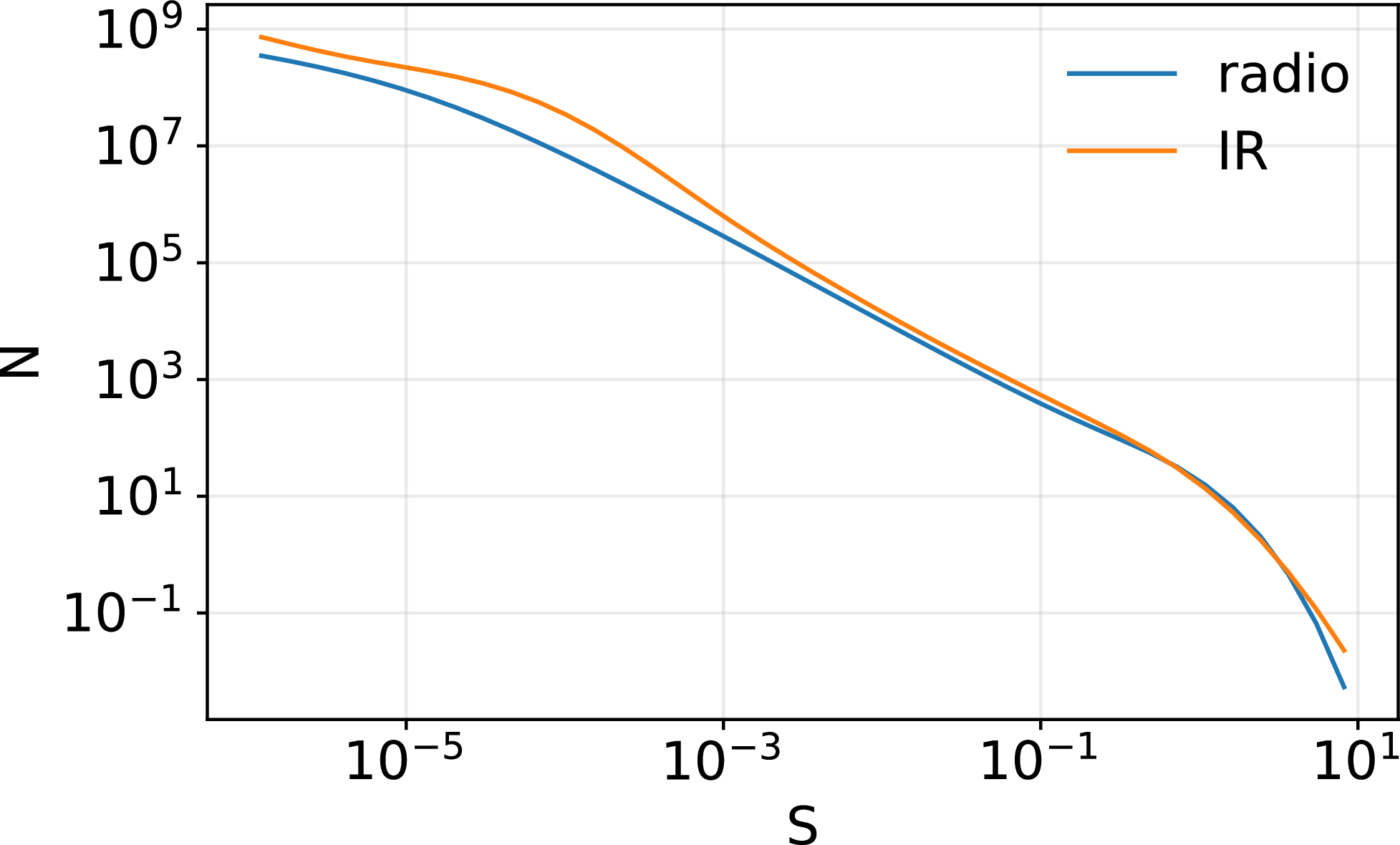
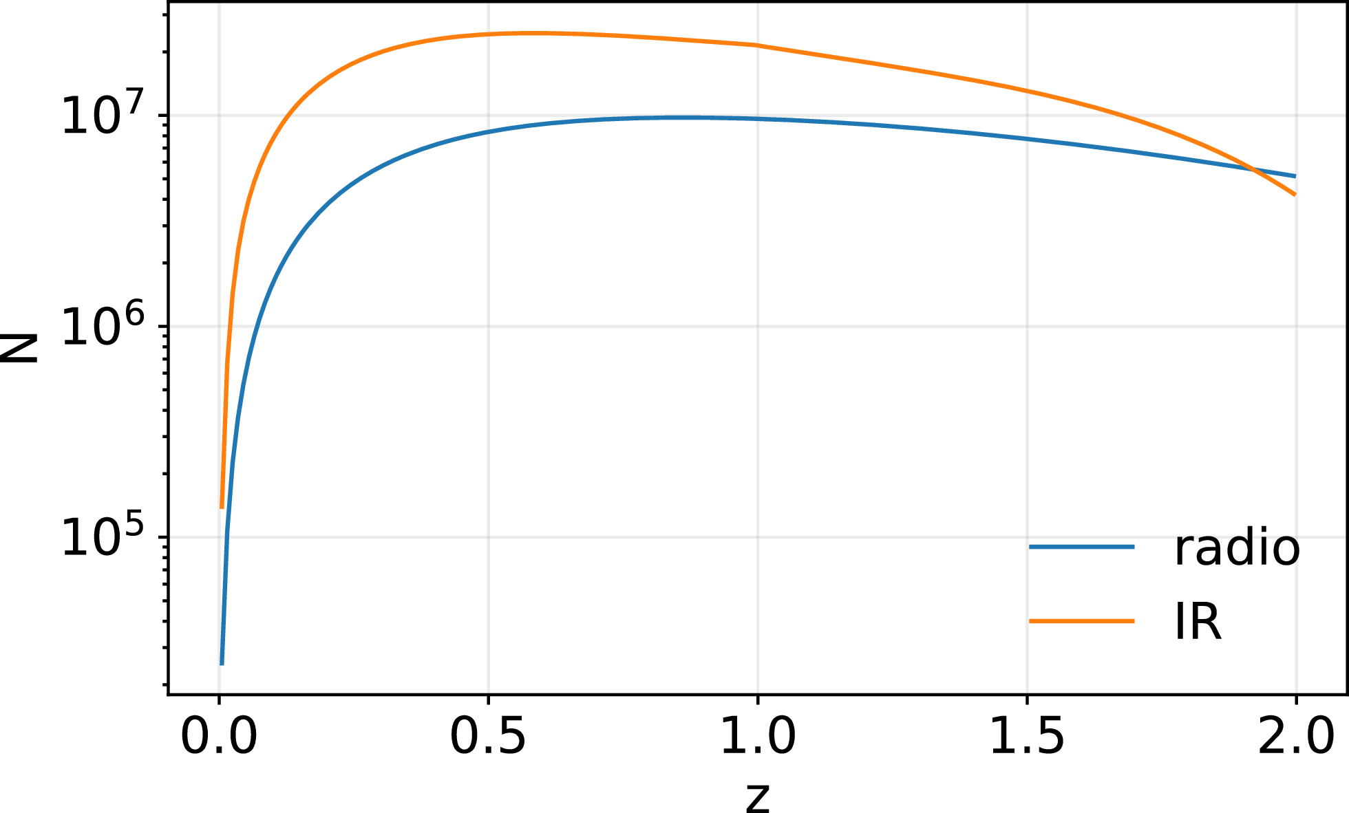
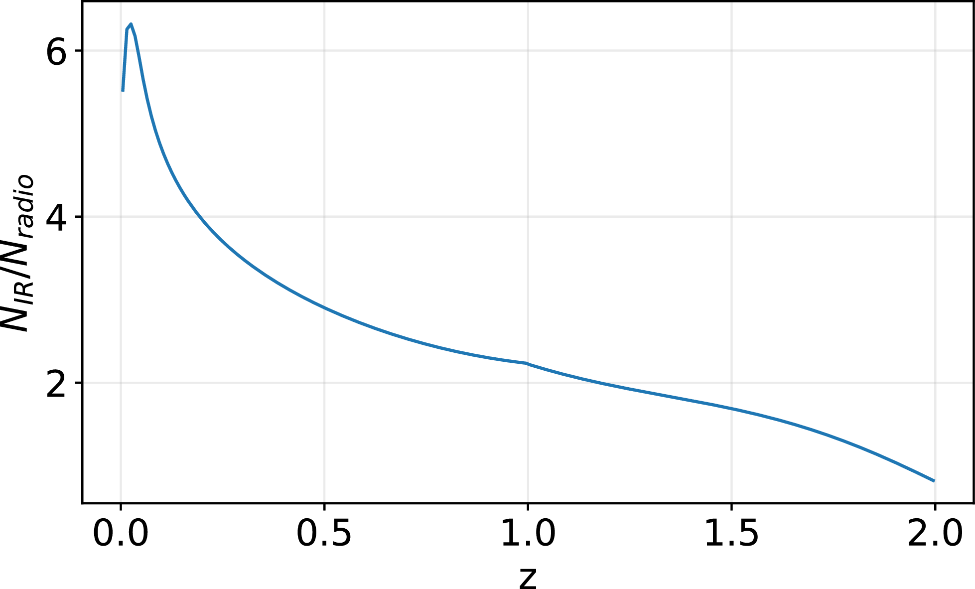
 z≲2
z≲2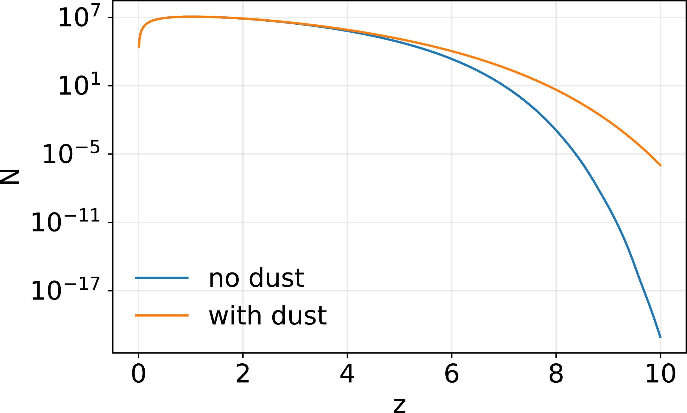
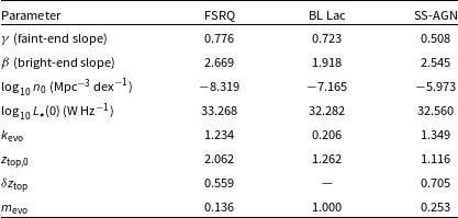
 γ
γ β
β kevo
kevo ztop,0
 δztop
δztop mevo
mevo
 Open access

