1.1 Population quantities

Suppose we are interested in public opinion on J binary outcomes. Our estimands $\theta ^j$ denote the population share holding attitude j. Superscripts index issues; subscripts index groups or individuals. For example, $\theta ^j$ might represent the share of the public who turn out to vote, who vote for the Democrat or who support a policy.

The population is partitioned into a set of cells $\mathcal {C}$ , where each cell c is defined by a combination of demographic variables and geography. For example, $\mathcal {C}$ might represent every combination of age, race, gender, education and county. Population cell sizes $N_c$ are known from Census data or other sources.Footnote ⁵ The total population is the sum of cell populations: $N \equiv \sum _c N_c$ . The poststratification table is defined by cell-level covariates and cell sizes $N_c$ . Because cells are defined by geography, let $\mathcal {C}_g$ denote the cells within geography g (e.g., $\mathcal {C}_{\text {Calif.}}$ for California).

Population opinion is a weighted average of cell-level opinion:

(1) $$ \begin{align} \text{population-level opinion:} \quad &\theta^j \equiv \frac{\sum N_c \theta_c^j}{\sum N_c} \nonumber\\\text{opinion in geography } g{:} \quad &\theta_g^j \equiv \frac{\sum_{c \in \mathcal{C}_g} N_c \theta_c^j}{\sum_{c \in \mathcal{C}_g} N_c}. \end{align} $$

1.2 MRP estimation

MRP estimation proceeds by using survey data to fit a regression model for $\theta ^j_c$ as a function of covariates in the poststratification table. The model typically includes geographic intercepts to capture remaining between-geography variation after accounting for individual-level covariates. The model is used to generate predictions $\hat {\theta }^j_c$ for each cell. After generating opinion estimates for each cell, researchers then poststratify those estimates to the geography of interest—that is, substituting estimates for the population quantities in Equation (1).

MRP allows researchers to estimate opinion in geographies that were not intentionally sampled. For example, researchers studying representation may want to know whether policy outcomes accord with public opinion (e.g., Lax and Phillips Reference Lax and Phillips2012; Tausanovitch and Warshaw Reference Tausanovitch and Warshaw2014), but even large surveys are unlikely to have many respondents in any given geography. MRP provides a solution by pooling information across geography and demographics via the regression step and accounting for differences in population composition via the poststratification step.

1.3 Remaining sources of error

The performance of the MRP estimates relies on ignorability: conditional on covariates, representation in the survey is independent of the outcome. Under ignorability and correct model specification, MRP is consistent. To make these assumptions more plausible, recent work has focused on specifying more complex interactions (e.g., Bisbee Reference Bisbee2019; Broniecki et al. Reference Broniecki, Leemann and Wuest2022; Ghitza and Gelman Reference Ghitza and Gelman2013; Goplerud Reference Goplerud2024) and increasing the number of poststratification variables (Leemann and Wasserfallen Reference Leemann and Wasserfallen2017). Still, respondents may differ from non-respondents in unobservable ways. Additionally, attempts to reduce bias by increasing model complexity may be offset by increased variance (Buttice and Highton Reference Buttice and Highton2013; Warshaw and Rodden Reference Warshaw and Rodden2012).

A second source of error arises when the population of interest differs from the population used to construct the poststratification table. An example is estimating the opinions of the electorate using the voting-age population demographics.

Finally, even under ideal conditions, MRP does not guarantee accurate estimates for every geography: model-based estimates that are unbiased overall can still produce sizable errors in specific areas.

3.1 Multivariate outcome model

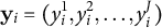
Recall that our estimand is opinion on J issues with true values $\theta ^j$ . For each respondent $i,$ we observe binary responses $y_i^j$ and demographic cell membership c. Each cell has a demographic covariate vector $\mathbf {x}_{c}$ and a geographic covariate vector $\mathbf {z}_{g[c]}$ . We model $y_i^j$ using a multivariate logit model with demographic and geographic covariates. We include a random intercept for each geography g. Conditional on covariates, responses across issues are assumed independent.

The model for each issue j is given by

(4) $$ \begin{align} \begin{aligned} y^j_i &\sim \text{Bernoulli}(\theta_{c[i]}^j) \quad \text{for } j \in 1, \dots, J\\ \theta_{c}^j &= \text{logit}^{-1}\left( \alpha_{{g}[c]}^j + \mathbf{x}_c'\beta^{j} + \mathbf{z}_{{g}[c]}'\gamma^{j} \right), \end{aligned} \end{align} $$

where $\beta ^j$ and $\gamma ^j$ are vectors of coefficients on the demographic and geographic predictors, respectively. The parameter $\alpha _{{g}[c]}^j$ is a random intercept for item j that varies by geography.Footnote ⁹ To permit partial pooling (Gelman and Hill Reference Gelman and Hill2007), we specify a hierarchical multivariate normal distribution for the random intercepts:

(5) $$ \begin{align} &(\alpha_{{g}}^1, \alpha_{{g}}^2, \dots, \alpha_{{g}}^J) \sim \text{MultivariateNormal}(\mathbf{0}, \boldsymbol{\Sigma}). \end{align} $$

The covariance matrix $\boldsymbol {\Sigma }$ , estimated from the data, encodes the within-geography correlation across outcomes after accounting for other model terms. We use $\boldsymbol {\Sigma }$ to predict logit shifts for outcomes without ground-truth data.

This model nests the traditional approach of estimating separate regressions for each outcome. This approach corresponds to constraining $\boldsymbol {\Sigma }$ to be diagonal—sharing no information about geographic random effects across outcomes.

3.2 Calibration procedure

We reinterpret the logit shift as the residual between the estimated random effect $\hat {\alpha }_{g}^j$ and the realized geographic intercept. Substitute Equation (4) into the expression for the updated cell-level probabilities after calibration in Equation (3):

$$ \begin{align*} \tilde{\theta}^{j}_c &= \text{logit}^{-1}\left(\delta_{g[c]}^j + \text{logit}(\hat{\theta}_c^j) \right) \\ &= \text{logit}^{-1}\left(\smash{\underbrace{\delta_{g[c]}^j + \hat{\alpha}_{{g}[c]}^j}_{\text{realized intercept}}} + \mathbf{x}_c' \hat{\beta}^{j} + \mathbf{z}_{g[c]}' \hat{\gamma}^{j} \right). \end{align*} $$

Because the updated probabilities ensure that model-implied geographic estimates match observed ground truth, the logit shift $\delta ^j_g$ can be interpreted as the residual between the estimated intercept $\hat {\alpha }_g^j$ and the realized intercept $\delta ^j_g + \hat {\alpha }_g^j$ .

This perspective suggests a method for predicting logit shifts for outcomes with unknown ground truth. We invoke a covariance equivalence assumption: the covariance of $\delta _g^j$ equals the covariance of geographic random intercepts estimated from the survey. More formally, we assume $(\delta _g^1, \dots , \delta _g^J) \sim \text {MultivariateNormal}(\mathbf {0}, \boldsymbol {\Sigma })$ , where $\boldsymbol {\Sigma }$ is the same as in Expression (5). The upshot of this assumption is that we can use the survey to estimate the correlation in realized random effects.Footnote ¹⁰

We observe logit shifts for the auxiliary variables with ground-truth data. Denote the vector of observed logit shifts $\delta _g^{\mathbf {o}}$ and the vector of unknown logit shifts $\delta _g^{\mathbf {u}}$ . Conditional on the observed shifts, the expected value of unobserved logit shifts has a linear formFootnote ¹¹:

(6) $$ \begin{align} E[\delta_g^{\mathbf{u}} \mid \delta_g^{\mathbf{o}}] &= \boldsymbol{\Sigma}_{\mathbf{uo}} \boldsymbol{\Sigma}_{\mathbf{oo}}^{-1} \delta_g^{\mathbf{o}}. \end{align} $$

In this equation, $\boldsymbol {\Sigma }_{\mathbf {uo}}$ is the cross-covariance in random effects between the unobserved and observed elements and $\boldsymbol {\Sigma }_{\mathbf {oo}}^{-1}$ is the inverse of the covariance of the observed elements. This expression follows from the properties of the multivariate normal distribution (Eaton Reference Eaton2007, 116).

In other words, the logit shift parameters for the outcomes without ground-truth data are a linear combination of the logit shifts for the outcomes with calibration data. The coefficients in this linear combination depend on the covariance in the geographic random effects across outcomes, with higher weights going to the logit shift of outcomes with higher covariance.

To build intuition, consider the case of a single observed auxiliary outcome ( $j=1$ ) and a single unobserved outcome ( $j=2$ ). The predicted logit shift is $E[\delta ^2_g\mid \delta _{g}^{1}] = \rho \frac {\sigma _{2}}{\sigma _1} \delta _g^1$ , where $\rho $ is the correlation between random effects and $\sigma _1$ , $\sigma _{2}$ are their standard deviations. The correlation controls the magnitude, while the ratio of standard deviations corrects for scale differences. If $\rho = 1$ , the logit shift for the unobserved outcome equals the observed shift (up to a scale adjustment). If $\rho = 0$ , the observed shift is uninformative and no adjustment is made.

3.3 Assumptions and limitations

In this section, we discuss several points related to the covariance equivalence assumption, which we rely on to derive the estimator.

First, this assumption could be violated if respondent correlations differ from those in the population. For example, because survey respondents are often highly educated and more politically interested than the public, their attitudes may be more correlated across issues than those of the general public (Freeder, Lenz, and Turney Reference Freeder, Lenz and Turney2018; Hopkins and Gorton Reference Hopkins and Gorton2023; Marble and Tyler Reference Marble and Tyler2022). Although strong, this assumption is almost certainly better than the traditional MRP default, which implicitly assumes no correlation. Other weighting methods make similar assumptions: raking, for example, can over-correct when the sample correlation between an underrepresented group and the outcome exceeds the population correlation.

Second, the scale of the random effects estimated in the survey might differ from the scale of the true intercept shifts needed for calibration. This form of error affects inferences only when there is differential error in the survey-based estimate of the variances in $\boldsymbol {\Sigma }$ across outcomes. To be more precise, consider the scale-correlation factorization of $\boldsymbol {\Sigma } = D \Omega D$ , where $\Omega $ is the correlation matrix and ${D = \text {diag}(\sigma _1, \dots , \sigma _J)}$ are standard deviations. If our estimate of each element of D is off by a common factor, such that $\hat {D} = k D$ for a scalar k, then the point estimates of our method are unaffected, but if different elements of D are estimated with differential error, it could lead to over- or under-updating.

Appendix F of the Supplementary Material discusses these points further and provides empirical evidence for the plausibility of the covariance equivalence assumption in our application.

3.4 Estimation

Estimation proceeds by first fitting the multivariate model in Equations (4) and (5) to survey data. Next, we poststratify and calculate logit shifts for outcomes with ground truth following Equation (2). Finally, we apply Equation (6) to update the remaining outcomes.

The simplest option is a plug-in estimator for $\boldsymbol {\Sigma }$ (e.g., the MLE or posterior mean). In our application, we adopt a fully Bayesian approach. For each posterior draw, calculate logit shifts for observed outcomes; predict implied shifts for unobserved outcomes; update unobserved outcomes; and, finally, poststratify. We summarize results using the posterior mean. See Appendix A of the Supplementary Material for a formal description.Footnote ¹²

3.5 Comparison with alternative approaches

Our procedure uses observed estimation error in a subset of outcomes to adjust others. Several alternative approaches exist, which we briefly discuss here and more fully in Appendix D of the Supplementary Material.

First, classic weighting methods like raking can use known margins as weighting targets. But, without an outcome model, the survey must contain respondents from each geographic unit, making it infeasible for estimating opinion in small subgroups. Second, known margins can be included as geographic predictors in the regression. This approach likely improves estimates, but it does not guarantee that they match known margins. Our calibration procedure can be applied in conjunction with this approach to reduce remaining error. Third, researchers can generate synthetic poststratification tables (MRsP; Leemann and Wasserfallen Reference Leemann and Wasserfallen2017). The Supplementary Material discusses two variants: assuming conditional independence between demographics and the calibration variable (“conventional MRsP”) or using a first-stage calibrated MRP model as the poststratification table for a second stage (“chained calibrated MRP”). Our approach sidesteps the need to impute this poststratification table, and instead estimates multiple outcomes jointly.

3.6 Extension to hyperlocal geography

Our approach can be extended to smaller geographies lacking poststratification data but with ground-truth calibration data. For example, we can use it to estimate opinion in precincts, where election results are available but poststratification data are not. To do so, we initialize precinct-level predictions to their corresponding county-level values. We then calibrate using observed precinct-level vote share, assuming the precinct-level correlation structure matches the estimated county-level structure. While this assumption need not hold—particularly if there is significant heterogeneity across precincts within counties—in our application it performs well. This extension enables hyperlocal opinion estimation even without poststratification data or fine-grained geographic identifiers in the survey. Appendix H of the Supplementary Material describes this extension further and validates its performance.

4.1 Validation approach

We model vote choice for the three statewide elections (alongside other opinions) as a function of respondent- and county-level predictors. We first generate uncalibrated county-level estimates by poststratifying on the joint distribution of county demographics. We then calibrate to observed county-level margins for the Governor and Secretary of State races and assess how this changes estimation error.

Individual-level predictors include age, race, gender and education, with interactions between race $\times $ education and nonwhite $\times $ education $\times $ age. County-level predictors are percent nonwhite, percent Hispanic/Latino, percent college-educated, median income and 2020 Biden two-party vote share. The specification includes county-level random intercepts correlated across outcomes, which provide the basis for our adjustment. Further modeling details, including R code, are included in Appendix B of the Supplementary Material.Footnote ¹⁴

We produce two sets of adjusted results: the first calibrates Secretary of State and Proposition 3 using gubernatorial results; the second calibrates Proposition 3 using both gubernatorial and Secretary of State results.

Because we calibrate to two-party vote share, the calibration implicitly targets the electorate rather than the population. The approach can target the population instead by including turnout as a calibration variable—that is, calibrating to Democratic vote share, Republican vote share and aggregate turnout as functions of total population. We take this approach in a simulation study in Appendix I of the Supplementary Material. Researchers should take care in specifying the population of interest—which depends on the substantive research question—and ensuring that the calibration variables are measured accordingly.

4.2 Validation results

Calibration substantially reduces error: average absolute error for Secretary of State and Proposition 3 falls by $65\%$ and $60\%$ , respectively.

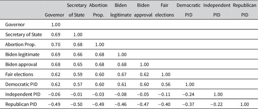
Table 1 reports correlations between county-level random intercepts across outcomes. This matrix measures residual within-county correlation on the logit scale after accounting for covariates.

Table 1

Correlation of county intercepts across outcomes, Michigan 2022

Note: Posterior mean correlations between county random intercepts across survey outcomes.

Consistent with partisan and geographic sorting, county intercept correlations are relatively high across outcomes. The sole exception is independent party identification, which is largely unrelated to other county-level opinions.

Despite these high average correlations, Table 1 reveals interesting variation. For example, the residual geographic correlation between governor vote choice and belief that Biden won legitimately is just below $0.7$ , but the correlation between governor vote choice and Republican party identification is about $-0.5$ . Calibrating to gubernatorial results will thus produce a smaller update for party identification than for beliefs about Biden’s legitimacy. In short, gubernatorial vote choice carries more information about opinions on Biden’s legitimacy than about party identification. This is consistent with the specifics of the race: Republican gubernatorial candidate Tudor Dixon denied Biden’s 2020 victory, alienating some Republicans (Ulloa Reference Ulloa2022).

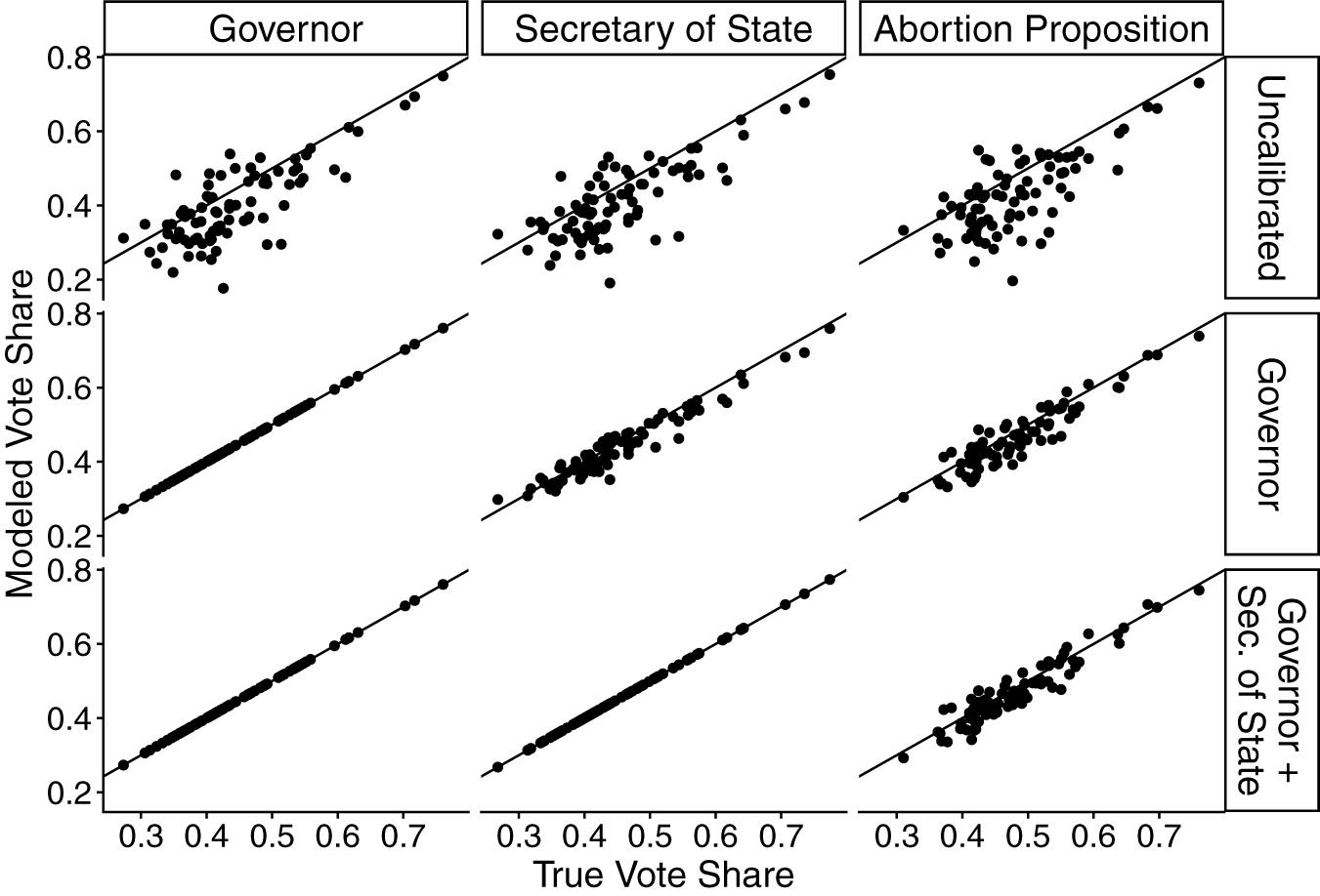
Using these correlations, we calibrate to outcomes with known county-level values. Figure 1 plots true county-level vote share against: (1) uncalibrated MRP estimates; (2) estimates calibrated to gubernatorial results; and (3) estimates calibrated to both gubernatorial and Secretary of State results.

Figure 1

County-level MRP results, Michigan 2022 elections.

Note: The x-axis shows the true county-level Democratic/pro-choice vote share and the y-axis shows model-based estimates. The top row shows uncalibrated MRP estimates, the middle row shows estimates calibrated to the Governor race and the bottom row shows estimates calibrated to Governor and Secretary of State races.

The top row shows that uncalibrated MRP underestimates Democratic vote share in the gubernatorial and Secretary of State races, as well as the pro-choice position in Proposition 3. Moreover, there is evidence of heteroskedasticity, with more variation in polling errors in less-Democratic counties. Some errors in less-Democratic counties exceed 10 percentage points.

The second row shows the effect of calibrating to gubernatorial results, showing a dramatic improvement in accuracy. By construction, calibrated gubernatorial vote shares perfectly match actual outcomes (far left). The center and right panels show that Secretary of State and Proposition 3 predictions also improve substantially. Calibrated estimates are closer to the 45-degree line and heteroskedasticity is greatly reduced.

The final row shows calibration using both Governor and Secretary of State results. As the panel in the lower-right reveals, the doubly-calibrated estimate is slightly improved relative to the estimates calibrated using only the gubernatorial results. The mild gains likely reflect the similar relationships both elections have with Proposition 3 support. The correlation of county intercepts between the Governor and Secretary of State races was nearly 0.7, indicating that the latter race adds relatively little additional information.

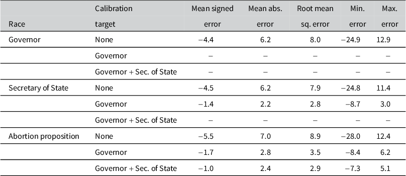
Table 2 summarizes these results by calculating the mean signed error, the mean absolute error (MAE), the root mean squared error (RMSE) and the range of errors across counties. Each panel has three rows: uncalibrated MRP, calibrated to Governor and calibrated to both Governor and Secretary of State.

Table 2

County-level errors, Michigan 2022 elections

Note: Entries in the table show the county-level error associated with uncalibrated and calibrated MRP vote share estimates for the Democrat/pro-choice outcome. The first row for each race is the error when using uncalibrated MRP; the second row is the error when calibrating to the Governor outcomes and the third row is the error when calibrating to both the Governor and Secretary of State outcomes.

Figure 2

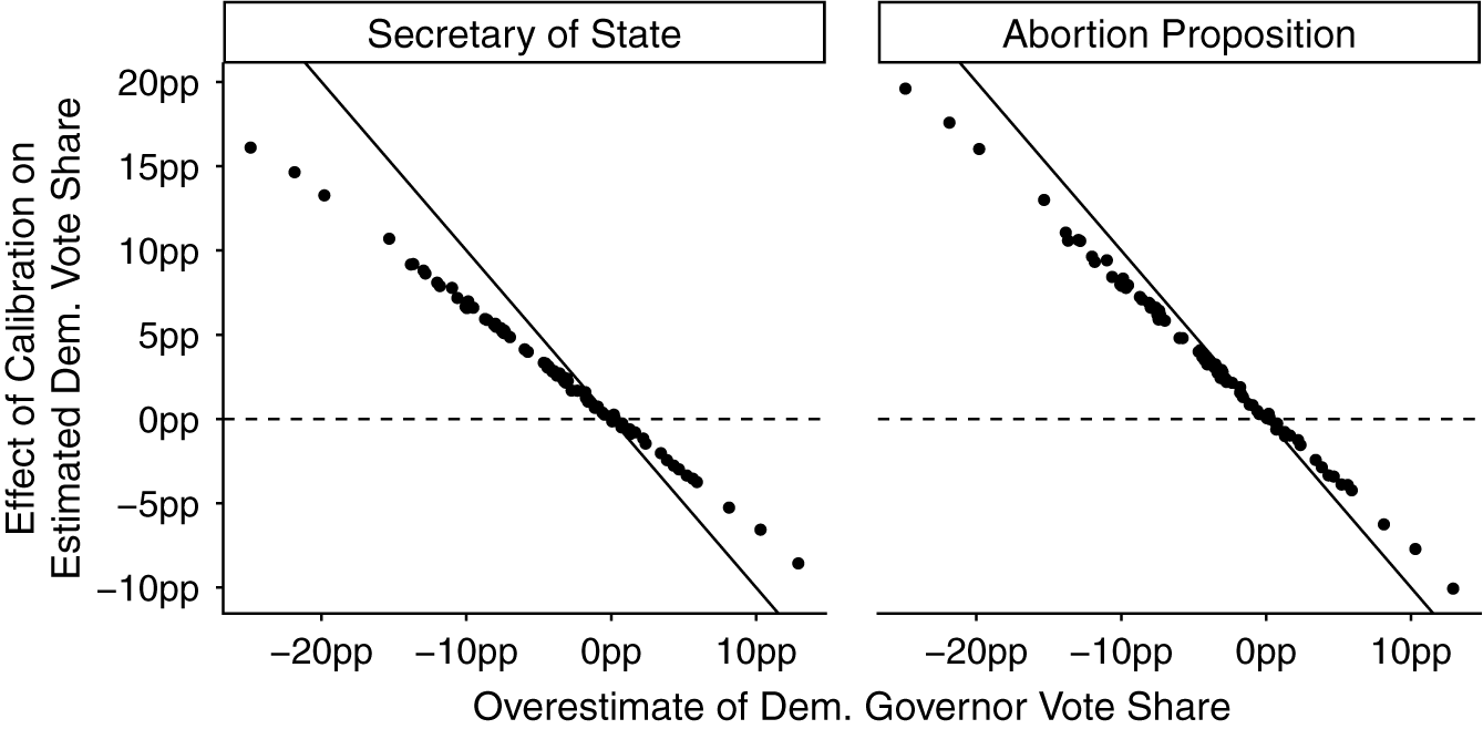
Change in county-level estimates from calibration to Governor results.

Note: The y-axis plots the difference between calibrated and uncalibrated county-level estimates for Secretary of State and the abortion proposition. The x-axis shows the county-level error in the Governor’s race before calibration where positive values indicate overestimating the support for Democratic incumbent Gretchen Whitmer.

Calibrating to the Governor race reduces mean signed error in the Secretary of State race from $4.5$ percentage points in the Republican direction to just $1.4$ points—a reduction of $69\%$ . MAE and RMSE both fall by nearly two-thirds and the error range shrinks dramatically, from $[-24.8,11.4]$ to $[ -8.7, 3.0]$ .

Proposition 3 results show modest additional gains from calibrating to multiple outcomes. The MAE is reduced from $7.0$ to $2.8$ percentage points when calibrating to the Governor results—a reduction of $60\%$ . Jointly calibrating to both races further reduces the MAE to $2.4$ percentage points. Maximum and minimum errors are also greatly reduced by calibrating to both races.

To visualize the nature of the calibration, Figure 2 plots the effect of calibration in the Secretary of State and abortion proposition against the baseline error in estimates for Governor.Footnote ¹⁵ The x-axis shows the gubernatorial overestimate; the y-axis shows the change in estimates after calibration.

The pattern is intuitive: where standard MRP overestimates gubernatorial Democratic vote share, other estimates are revised downward. Most points fall below 0 on the x-axis—indicating that baseline MRP underestimates Democratic vote share. Consequently, most observations fall above 0 on the y-axis.

The slope reflects the cross-race correlations. One-for-one adjustment would place points on the 45-degree line. The observed slope is flatter, reflecting imperfect correlations across races. The fact that the left-hand panel has a flatter slope than the right-hand panel reflects the lower correlation between the Governor and Secretary of State races than between the Governor race and the abortion proposition.

In sum, we find that our calibrated MRP approach can significantly improve estimates of small-area opinion. We compare our approach to alternatives in Appendix E of the Supplementary Material, finding that our method outperforms alternatives in this setting. In Appendix J of the Supplementary Material, we also show the effect of calibration on party identification—an outcome with no ground-truth data in Michigan.