1. Introduction
In the present era of multi-wavelength (in fact, multi-messenger) astronomy, the sky remains poorly explored at the very low radio frequencies, particularly below 20 MHz. The radio sky at such low frequencies would be expected to be very bright due to the dominance of non-thermal emission; however, there would also be rapidly increasing free–free absorption from intervening thermal plasma. The sky images at these frequencies would, therefore, be expected to offer an unprecedented opportunity to probe both of these contributors, through the spectral evolution of their combined effect, which is not possible to infer from trivial extrapolation of available measurements at the higher frequencies. However, ground-based observations of astronomical sources in this spectral band are severely limited owing to the spectral cut-off due to the Earth’s ionosphere and also suffer from spectral contamination by man-made radio frequency interference (RFI).
To overcome these constraints, such radio observations have already been attempted from above the ionosphere but were initially limited to using a single antenna set-up, with no significant angular resolution. To image the radio sky from space with angular resolutions comparable to those routinely achieved in ground-based observations at higher radio frequencies, we would necessarily need to appeal to the aperture synthesis technique, using multi-element space interferometers. Even if aperture sizes of the individual elements may be relatively small, due to practical considerations, implying limited instantaneous sensitivity, significantly finer resolution angular resolution can be achieved, equivalent to that of an Earth-size aperture:
 \begin{equation} \theta_{arcsec} \approx 0.6\frac{(\lambda_{m}/30\,\text{m})}{(D_{km}/10\,000\, \text{km})},\\ \end{equation}
where $\theta_{arcsec}$
is the angular resolution of the telescope, expressed in arcsecond,
$\theta_{arcsec}$
is the angular resolution of the telescope, expressed in arcsecond, $\lambda_{m}$
is the wavelength in metres, and
$\lambda_{m}$
is the wavelength in metres, and $D_{km}$
is the size of the effective aperture synthesised (or the maximum baseline length in case of interferometry) in km.
$D_{km}$
is the size of the effective aperture synthesised (or the maximum baseline length in case of interferometry) in km.
Orbiting Very Long Baseline Interferometry (OVLBI) is not a new concept to radio astronomers and has been employed multiple times in the past (see e.g., Gurvits (Reference Gurvits2018)). Multi-element space-based radio interferometers have been used, but only in conjunction with ground-based telescopes, therefore, rendering them unusable for observations in the lower frequency window. For example, the first ever mission to have operated in space providing us the proof of concept of OVLBI was the Tracking and Data Relay Satellite System (TDRSS), from 1986 to 1988 (see Teles et al. (Reference Teles, Samii and Doll1995)). Following that came the Space VLBI Satellite: MUSES-B (see Hirabayashi et al. (Reference Hirabayashi1998)) under the Japanese VLBI Space Observatory Program (VSOP) and RadioAstron (Spektr-R, see Kardashev et al. (Reference Kardashev, Kovalev and Kellermann2012)) operated by the Russian Astro Space Center. Similarly, the Chinese Cosmic Microscope is another proposed Earth–space VLBI mission with two satellites, though at high frequencies (see An et al. (Reference An2020)).
The increasing interest in radio sky at very low frequencies has, in the past few decades, resulted in several space-interferometric missions being proposed (such as SURO, OLFAR; see Baan (Reference Baan2013), Engelen et al. (Reference Engelen, Verhoeven and Bentum2010), Bentum et al. (Reference Bentum2020), and references therein). These proposed swarms of small satellites (close to the Earth or at other special locations within our solar system, such as L2 or lunar orbit) would have a large number of apertures working together in aperture synthesis mode, but with baseline lengths limited to 100 km or so.
It is clear that sensitive imaging observations with very high angular resolution at such low frequencies possess immense potential to reveal the yet unexplored view of the entire radio sky. Motivated by these prospects, a suitable space interferometer system to enable such high-resolution imaging is considered.
Our exploration and identification of a novel minimal configuration consisting of three apertures in Low Earth Orbit (LEO), which is the focus of the present study, is only the first step towards the design and development of such a system. We consider a radio astronomy payload on each satellite as consisting of a suitable antenna providing a very wide field of view (FoV). Such a configuration would allow us to sample baselines of over 15000 km, which is larger than the diameter of the Earth, thus enabling angular resolution as fine as 1 arcsec even at 4 MHz.
Here, it is worth noting the difference between (usually stationary) interferometers on the Earth and those formed by moving apertures in LEO, in terms of the speeds of both the (u,v) coverages and access to sky area. For interferometers on the Earth, the rate of change of projected baselines (i.e., the (u,v) spacing) is dictated by the rotation rate of the Earth, and the chosen set of aperture locations, where the typical duration required to sample the available spacings is about half a day, for most sky directions in the view. Similarly, unless the Earth-based interferometers are spread over the entire globe, access to different areas of the sky, bringing them within the field of view of the apertures, is again dictated by the Earth rotation, where mere viewing of the entire sky, if at all possible, will require at least half a day, even with a very wide FoV. Both these aspects together imply a 1-day cycle for relevant measurements across the entire accessible sky. In contrast, each of the apertures in LEO, with adequately wide (say, hemispheric) FoV, can access effectively the entire sky in the duration of a single orbit, which is are an order of magnitude shorter than a day.
As for interferometers using apertures in LEO, the preliminary implications of orbital periods are also worth noting. Let us consider both cases, short- and long-period orbits. Shorter the orbital periods, faster will be the realisation of the sequence of baselines possible with a given pair of orbits, implying in turn, a faster (u,v) coverage. However, the available integration time for visibility measurement at a given (u,v) spacing is correspondingly reduced. To ensure the amount of integration in a given (u,v) cell to be same in both cases, correspondingly more cycles of revisit to the cell are required in case of faster orbits, and as would be expected, the total time span requirement tends to be independent of the orbital periods.
In this paper, we describe our simulation of a system consisting of small apertures aboard multiple LEO satellites for observations of the entire sky at low radio frequencies. We begin with a minimal system consisting of three satellites in mutually orthogonal orbits and show that this configuration gives desired spatial frequency (u,v) coverage of the entire sky. We perform multiple tests by varying the (relative) phase and period of the orbits of the satellites to assess improvements in the performance in terms of (u,v) coverage. Our system consists of one satellite orbiting the Earth in the equatorial orbit, while the other two satellites are in mutually perpendicular polar orbits. Each of the satellites has an orbital height which is slightly different from the other two, which results in a different (non-redundant) baseline at different points of time, thus greatly improving sampling in (u,v) plane. We quantitatively evaluate the upper and lower limits of the percentage coverage, or the filling factor, in the (u,v) plane achievable for different possible source directions, by considering a few extreme cases of relative source direction. The sensitivity of the (u,v) coverage is also assessed by varying the orbit and the initial phase of the satellites. We discuss the results obtained from these simulations and highlight the advantages of such a system.
Section 2 describes the model, including the parameter definition, the governing equations, and the main assumptions. Section 3 presents the analytical results, with separate subsections for results related to different objectives and different special cases. In Section 4, we first discuss some of the assumptions relating to our model, their validity, and implications. Before concluding, we touch upon some of the challenges relating to RFI, synchronisation, and data rates, as relevant to interferometry.
2. A space interferometer configuration: Our model
Here, we describe our model configuration for a space interferometer, presenting the governing equations and defining the various relevant parameters to make the model as realistic as possible. We also state the assumptions made and related justifications, including how the (u,v) plane has been defined for our fully space-based configuration.
Our model configuration is defined in a reference coordinate system with its origin at the centre of the EarthFootnote
a
. As can be readily visualised, employing only two satellites with fixed geocentric orbits, regardless of their orbital parameters, would not be sufficient to map the entire sky, even when each of their radio astronomical antennas have a FoV of as much as $2\pi$
steradians (refer to Figure 1). Hence, our starting model consists of three satellites in mutually orthogonal orbits; one in equatorial orbit and the other two in mutually orthogonal polar orbits. These orbits have their axes along the x, y, and z axes of the reference coordinate system.
$2\pi$
steradians (refer to Figure 1). Hence, our starting model consists of three satellites in mutually orthogonal orbits; one in equatorial orbit and the other two in mutually orthogonal polar orbits. These orbits have their axes along the x, y, and z axes of the reference coordinate system.
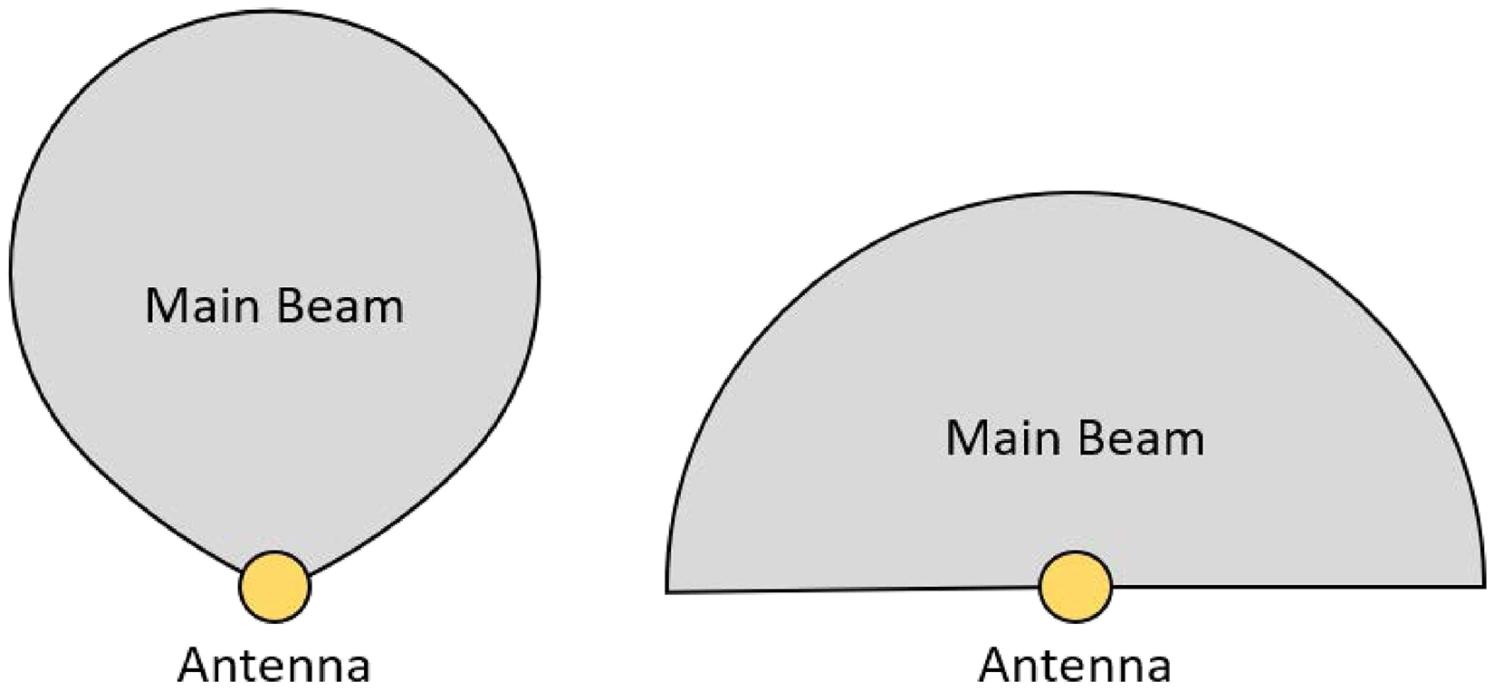
An illustration contrasting the typical main beam of a usual wide-field radio astronomical antenna (left) with the semi-isotropic beam (right) of a special antenna (system) considered in our model.
The number of interferometric baselines is given by:
 \begin{equation} n_b = \frac{n(n-1)}{2}, \end{equation}
where n is the number of antennas in the system. Thus, in our model with three antennas, the number of possible baselines would also be three.
We consider all three orbits to be different from each other, with different orbital heights (measured from the surface of the Earth), making their orbital periods distinctly different, and the heights are deliberately chosen such that the orbits are mutually asynchronous. The latter ensures that the apparent baselines are different during each orbital cycle, thus giving us significantly filled (u,v) coverage in a relatively short time span.
In general, the satellites would orbit around the Earth in elliptical orbits, with the Earth centre being at one of the two foci. The magnitude of the velocity (or the orbital speed) of a satellite in this general case is given by:
 \begin{equation} s = \sqrt{GM_e(\frac{2}{r}-\frac{1}{a})}, \end{equation}
where G (= $6.67 * 10^{-11} \, {\rm{N}}{\rm{m}}^2/{\rm{kg}}^2$
) is the universal gravitational constant,
$6.67 * 10^{-11} \, {\rm{N}}{\rm{m}}^2/{\rm{kg}}^2$
) is the universal gravitational constant, $M_e$
(=
$M_e$
(= $5.982*10^{24} {\rm{kg}}$
) is the mass of the Earth, r is the instantaneous radial distance of the orbiting satellite from the Earth centre, and a is the semi-major axis of the elliptical orbit. In our model, we have assumed, for simplicity, the LEO satellites to be in a nearly circular orbit (i.e.,
$5.982*10^{24} {\rm{kg}}$
) is the mass of the Earth, r is the instantaneous radial distance of the orbiting satellite from the Earth centre, and a is the semi-major axis of the elliptical orbit. In our model, we have assumed, for simplicity, the LEO satellites to be in a nearly circular orbit (i.e., $a \approx r$
), so as to improve the uniformity in (u,v) coverage in both dimensions. Therefore, the average magnitude, s of the satellite velocity would be,
$a \approx r$
), so as to improve the uniformity in (u,v) coverage in both dimensions. Therefore, the average magnitude, s of the satellite velocity would be,
 \begin{equation} s \approx \sqrt{\frac{GM_e}{r}}, \end{equation}
and the corresponding orbital period T,
 \begin{equation} T \approx \frac{2 \pi r}{s}, \end{equation}
where $r = R + h$
, R (=
$r = R + h$
, R (= $6\,371 \,\text{km}$
) is the radius of the Earth and h is the height of the orbit above the Earth surface.
$6\,371 \,\text{km}$
) is the radius of the Earth and h is the height of the orbit above the Earth surface.
The Earth gravity dominates, as expected, the considerations that dictate the geocentric motion of the satellites, and in comparison, any effects of, particularly, the Sun and the Moon and other solar system bodies can be ignored. Noting the long timescales associated with nutation, and even longer for precession (see, Balmino (Reference Balmino1974)), compared to the timescales relevant to obtaining desired (u,v) coverage, these two effects are not included in our model. Of course, the apparent astronomical source coordinates (such as RA and Dec) which are defined with reference to Earth rotation, do routinely need to take into account the evolution of the Earth’s spin axis. Also, the effects due to the apparent forces, such as the Coriolis force (arising as a result of the Earth’s rotation), those related to atmospheric drag, tidal effects, solar wind pressure, etc., are relatively small (see for more details, Balmino (Reference Balmino1974)) and are therefore not considered. Even though some of these effects might be significant in the long-term operability of the satellites, and the apparent directions of the source may be redefined in the equatorial coordinate system as the spin axis of the Earth on relevant long timescales, these aspects have little effect on how the mutual separation of the satellites would vary and the resultant spatial frequency coverage they provide.
Unless otherwise mentioned, the beam width or the FoV of each antenna is assumed, for simplicity, to be 180 $^{\circ}$
, or
$^{\circ}$
, or $2\pi$
steradians, respectively, even though in reality it is impossible to have such a sharp truncation in antenna response (refer to Figure 1). Usually, beam widths of typical antennas would be expected to be narrower. However, a near semi-isotropic beam can be achieved even with a short dipole with a reflector, or using a suitably arranged array of aperture elements, discussion of which is beyond the scope of the present theme. Our model does have a provision to consider narrower beam widths, but most of our simulations assume the default beam width, for the sake of computational efficiency.
$2\pi$
steradians, respectively, even though in reality it is impossible to have such a sharp truncation in antenna response (refer to Figure 1). Usually, beam widths of typical antennas would be expected to be narrower. However, a near semi-isotropic beam can be achieved even with a short dipole with a reflector, or using a suitably arranged array of aperture elements, discussion of which is beyond the scope of the present theme. Our model does have a provision to consider narrower beam widths, but most of our simulations assume the default beam width, for the sake of computational efficiency.
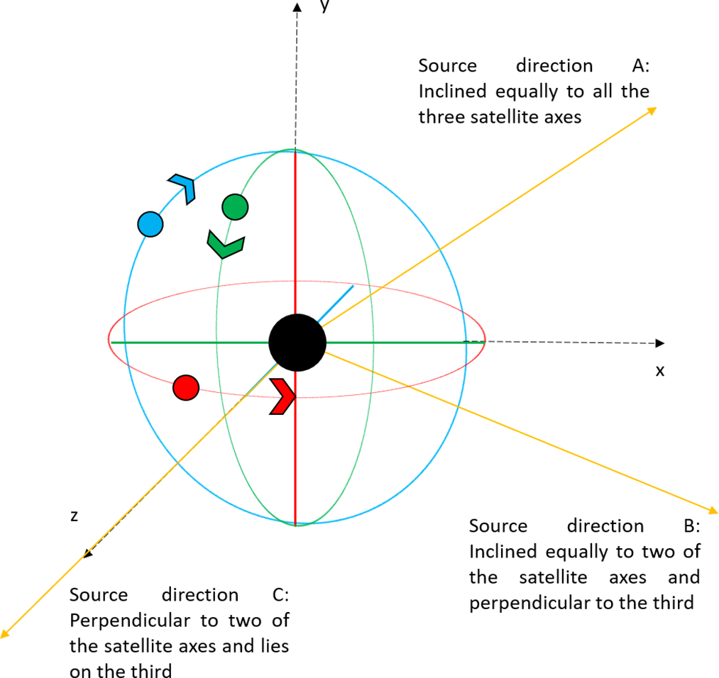
Figure 2 shows the essentials of our model configuration, with the Earth at the centre, along with the assumed coordinate system denoted by the x, y, and z axes. The satellites are shown in their orbits, with their orbit axes along the x, y, and z axes. Also indicated are the three distinct specific source directions for which the (u,v) coverage are assessed (as detailed in the beginning of Section 3).
An illustration of our model configuration: The near circular orbits (not to scale, and appearing in projection as ellipses) for the three satellites are shown. The first satellite has an equatorial orbit (red), and the other two (Satellite 2 and 3) have polar orbits (blue and green, respectively). The axes associated with the orbits coinciding with our 3D coordinate frame with its origin at the centre of the Earth (denoted by the black circle). The yellow rays indicate the three exclusive sky directions we consider (to be discussed in Section 3).
Our model parameters, which can be varied, include the orbital period (which in turn would change the orbital radius and the orbital velocity), as well as the starting orbital phase, of each of the satellites.
Although most of the distant astronomical sources have a unique direction, commonly defined as the Right Ascension (RA) and Declination (Dec), our simulations allow computation of spatial frequency (u,v) coverage even in the case of a relatively nearby source. Thus, in general, the source distance can be provided, in addition to the apparent direction (i.e., RA and Dec). By default, the source distance is assumed to be very large (say, $10^9$
AU or
$10^9$
AU or $\approx$
15 800 light years), unless specified otherwise.
$\approx$
15 800 light years), unless specified otherwise.
For a given direction RA and Dec, represented by $\alpha$
,
$\alpha$
, $\delta$
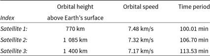
in radians, the 3D position of a source at finite distance,
$\delta$
in radians, the 3D position of a source at finite distance, $d_{source}$
, can be expressed as:
$d_{source}$
, can be expressed as:
 \begin{align} x_{source} &= (d_{source}*\cos(\delta))*\sin(\alpha) - x_{earth},\end{align}
 \begin{align} y_{source} &= (d_{source}*\sin(\delta)) - y_{earth},\end{align}
 \begin{align} z_{source} &= (d_{source}*\cos(\delta))*\cos(\alpha) - z_{earth}, \end{align}
where, $(x_{earth}, y_{earth}, z_{earth})$
define the Earth location w.r.t. the Barycenter of the Solar system and will vary depending on the phase of the Earth orbit around the Sun. For the distant sources (
$(x_{earth}, y_{earth}, z_{earth})$
define the Earth location w.r.t. the Barycenter of the Solar system and will vary depending on the phase of the Earth orbit around the Sun. For the distant sources ( $d_{source} \> \> AU$
), the above relations will reduce to the more familiar description of a unit vector (
$d_{source} \> \> AU$
), the above relations will reduce to the more familiar description of a unit vector ( $\hat{x}$
,
$\hat{x}$
, $\hat{y}$
,
$\hat{y}$
, $\hat{z}$
), in the direction of the source, neglecting the terms relating to the Earth’s orbital position, and normalisation by the distance
$\hat{z}$
), in the direction of the source, neglecting the terms relating to the Earth’s orbital position, and normalisation by the distance $d_{source}$
.
$d_{source}$
.
The (u,v) coverage obtainable in a time span, by default, of typically 16 days is simulated, unless a different span is specified. The observing time span of 16 days is chosen after extensive testing because having longer time periods does not provide any significant improvement in coverage.
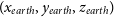
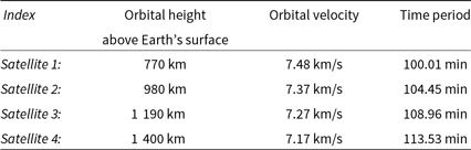
The various parameter values defined for each satellite are given in Table 1. Sensitivity of the (u,v) coverages to values of the listed (interdependent) parameters was examined by varying the relevant parameters.
Defined parameters of the model
The orbital height of Satellite 1 (in the closest orbit) is chosen to be greater than 700 km (in our simulations it is about 770 km) so as to be able to neglect the effects of atmospheric drag which may be substantial at orbital heights below 400 km and to also avoid attenuation of the radio waves due to the ionospheric plasma which is significant at orbital heights below 700 km (more about this is discussed in Section 4).
The orbital radii of Satellites 2 and 3 are larger by 315 and 630 km, respectively, than that of the Satellite 1, so as to realise as distinct baselines from the different pairs as possible, while still keeping the satellites well within the LEO limit, and having comparable time periods. The present values of the orbital radii are seen to give the best coverage, as evident from the tests described in the later sections, regardless of their starting orbital phases. Many other combinations of orbits at larger radii can also potentially provide similar coverages but would necessarily require correspondingly longer time spans.
Since our model is different from the usual Earth-based and Earth-and-space-based interferometer set-ups, we need to define the (u,v) plane explicitly in a suitable, though different, manner.
In order to do that, we have defined the (u,v) plane with its origin at the centre of the Earth, and the mutually orthogonal (unit) vectors, $\hat{u}$
and
$\hat{u}$
and $\hat{v}$
, are both also perpendicular to the chosen source direction (
$\hat{v}$
, are both also perpendicular to the chosen source direction ( $d_{source}$
; same as that of the unit vector
$d_{source}$
; same as that of the unit vector $\hat{w}$
).
$\hat{w}$
).
Following the usual convention, $\hat{v}$
always lies in the plane containing the source direction and the Earth rotation axis (i.e., both the north and the south poles).
$\hat{v}$
always lies in the plane containing the source direction and the Earth rotation axis (i.e., both the north and the south poles).
Note that the u and v values are presently expressed in km and not in the conventional units of wavelength. The Hermitian symmetric nature of the visibilities and the consequent symmetric sampling/coverage in the (u,v) plane are shown only in some of the figures. In other cases, only one sample point in (u,v) plane is counted/shown per baseline per time (instead of two due), to avoid cluttering in the display of coverage.
3. Simulation results and discussion
In this section, we examine and discuss the results of our simulation, in terms of the achievable (u,v) coverage, and dependencies on model parameters/configurations, assessed for a set of source directions.
During our simulations, we follow the locations of the satellites, to estimate the (u,v) spacings, at time interval of 10 s, and note the sampled spacing in the (u,v) plane spanning $\pm$
15 750 km. Although in such a time interval the baselines can change significantly, sometimes by as much as 100 km, the behaviour at finer time intervals, when required, can be found out to the desired accuracy directly, or even with suitable interpolation. This choice of time interval certainly makes the simulations computationally efficient, while still retaining the essential details of the (u,v) coverage for the purpose of illustration.
$\pm$
15 750 km. Although in such a time interval the baselines can change significantly, sometimes by as much as 100 km, the behaviour at finer time intervals, when required, can be found out to the desired accuracy directly, or even with suitable interpolation. This choice of time interval certainly makes the simulations computationally efficient, while still retaining the essential details of the (u,v) coverage for the purpose of illustration.
In order to simplify assessment of the maximum and minimum possible coverages achievable with our model system for any source direction, we define three special source directions (referred to as the three exclusive directions as in the Figure 2) for which we compute and examine the (u,v) coverage. These three special source directions, namely A, B, and C, are defined as follows:
-
1. Direction A: RA 03:00:00; Dec +45 deg, inclined equally to all three satellite orbit axes (equivalent situation would be encountered for RA of 9, 15, and 21 h, and/or declination of minus;45 deg).
-
2. Direction B: RA 03:00:00; Dec 0.0 deg, representing a set of specific directions that are perpendicular to one of the satellite orbit axes (or in the plane of that orbit) and inclined equally with the other two;
-
3. Direction C: RA 00:00:00; Dec 0.0 deg; perpendicular to any two of the satellite orbit axes and parallel to the third axis.
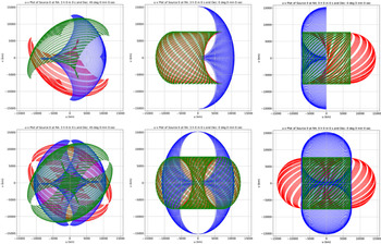
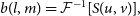
Figure 3 illustrates how the (u,v) coverage differs for each of three special source directions, estimated over a default span of 16 daysFootnote
b
. The situation for any other choice of source direction would typically be in between the cases equivalently represented by these three special source directions, and the (u,v) coverage would hence be also in between the range of baseline-wise coverages seen for the special source directions (a quantitative assessment of the coverages is provided in the Subsection 3.2). The u and v axes in these figures are shown in km rather than the usual wavelength ( $\lambda$
) units. Alternatively, the numerical values may be treated as referring to spatial frequencies, in units of the wavelength, at the radio frequency of 0.3 MHz, but can be scaled trivially to any other radio frequency.
$\lambda$
) units. Alternatively, the numerical values may be treated as referring to spatial frequencies, in units of the wavelength, at the radio frequency of 0.3 MHz, but can be scaled trivially to any other radio frequency.
The (u,v) coverages by the system of three satellites over the duration of 16 days, for the three pre-defined source directions. The top and the bottom rows of plots correspond to the (u,v) coverage without and with the inclusion of the sampling symmetry. The pair of plots in the three columns (left to right) refer to the three special source directions, namely the sources A, B, and C, respectively, as defined in the main text. The red, blue, and green tracks represent the baseline corresponding to the satellite pairs 1–2, 2–3, and 3–1, respectively. The u and v axes are indicated in km.

These results show that the system of three satellites renders sufficiently large coverage for all of the special source directions probed and can be expected to provide comparable coverage for other sky directions as well. If the primary FoV were to be narrower than assumed presently, the coverage would be correspondingly less extended, with little change in the detailed sampling of remaining region. A major or rather a dramatic adverse impact on the coverage should of course be expected when the narrowness of the FoV hampers any simultaneous observation of a given direction of interest by even one of the three satellites, with loss of two baselines. The directions which may fall outside those sampled by two satellites yield no coverage at all. Thus, the importance of ensuring that the equipment on each satellite is capable of observing over a sufficiently wide spread of directions (ideally $\pm 90^{\circ}$
) about their respective central (radial) directions cannot be overstated. This would require either a suitable multi-beam arrangement that allows a wide-field coverage collectively, or a single beam which can at least be steered to a chosen direction within the mentioned range, desirably without any reduction in the effective aperture/collecting area, facilitating a corresponding narrow-field measurement.
$\pm 90^{\circ}$
) about their respective central (radial) directions cannot be overstated. This would require either a suitable multi-beam arrangement that allows a wide-field coverage collectively, or a single beam which can at least be steered to a chosen direction within the mentioned range, desirably without any reduction in the effective aperture/collecting area, facilitating a corresponding narrow-field measurement.
We have also assessed if the attained coverage for a randomly chosen source direction would be qualitatively similar to the three cases presented. The related simulations indeed show a similar coverage span and fineness of sampling in (u,v), differing only in the overall orientation of the (u,v) tracks and the patch covered by the three interferometers, depending on the chosen direction.
Although for the presently discussed configurations, much of the potentially obtainable (u,v) coverage may be spanned in typically a few tens of days (e.g., 16 days), the considerations relevant for obtaining desired image quality are not limited to the span and fineness in (u,v) coverage, but necessarily include the various consistency checks between repeated observations, achievable sensitivity on long integrations, RFI detection and excision, calibratibility for various system parameters (in angular and spectral domains), understanding and accounting for systematics, etc. Ensuring image fidelity requires even more demanding considerations, which are beyond the scope of present paper, but are pivotal to reaching the sensitivity required for reliably detecting very weak signals, such as those related to the Epoch of Reionisation (see, e.g., the review by Liu & Shaw (Reference Liu and Shaw2020)).
3.1. Sensitivity of the (u,v) Coverage to the Orbital Parameters
The sensitivity of coverage to the two key parameters, namely the orbital period and orbital phase, is assessed separately. For these assessments, we probe the coverage for all of the three exclusive source directions but present only a few illustrative samples, all of them for source direction A, of the large ensemble of cases/combinations probed.
The sensitivity of coverage is assessed first by varying the orbital period of any one satellite at a time, keeping the orbital periods of the other two unchanged, and then repeating the procedure with the other two satellites. Since the orbital period of the satellite is directly related to its distance above the Earth, so we chose to vary these distances instead, and those values have been mentioned here henceforth. The corresponding orbital period can readily be computed using Equation (5).
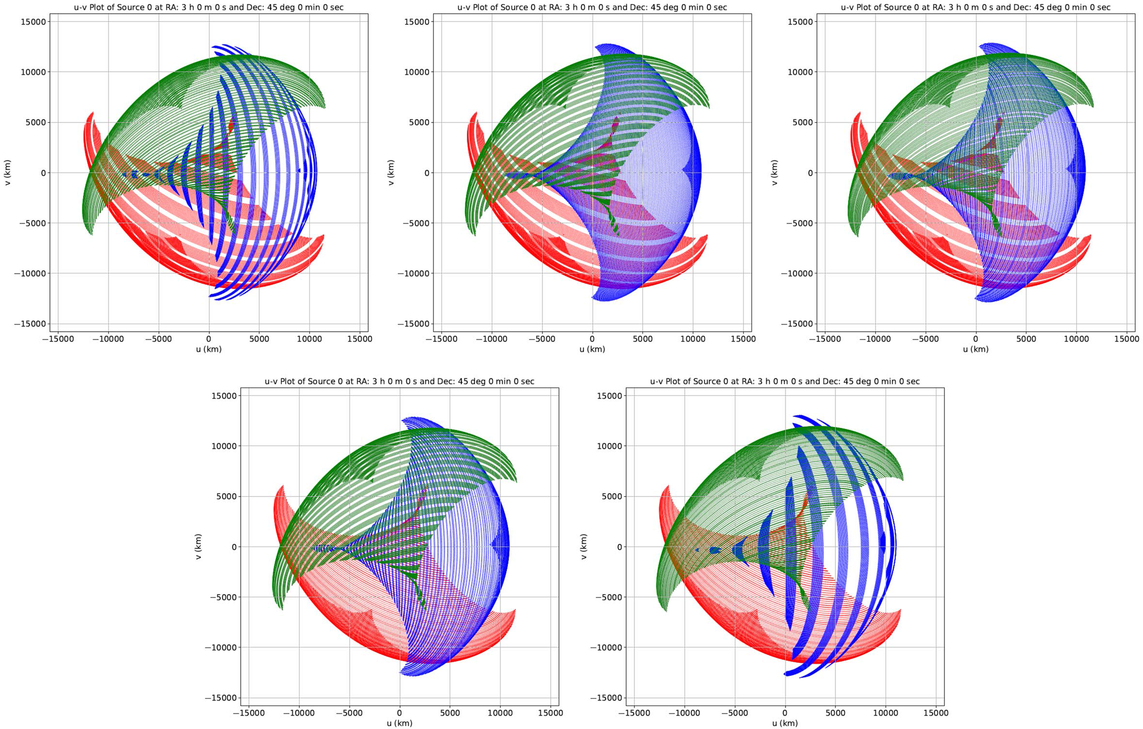
Figure 4 shows a few examples of the (u,v) coverage attainable in 16 days duration. Our results of these extensive assessment suggest that from among the different orbital distance combinations, the configuration in which the satellites 1, 2, and 3 are at 770, 1 185, and 1 400 km above the surface of the Earth, respectively, provides the maximum as well as most uniform spatial frequency coverage.
The (u,v) coverage obtainable in a 16-day time span for the source direction A is shown. For clarity, the symmetric counterpart of the coverage (implied by the Hermitian symmetric nature of the visibilities) is not displayed. The u and v axes are marked in km. A total of five configurations are shown for assessing sensitivity to orbital periods (corresponding to assumed heights). The height of the orbit of the Satellite 1 is kept constant at 770 km, while coverages in the top and bottom rows assume the height of the Satellite 2 orbit to be 1 085 and 1 185 km, respectively. In usual order, the plots correspond to the Satellite 3 height of 1 300, 1 400, and 1 500 km in the top panels, and 1 400 and 1 600 km in the lower panels. From among these cases, the coverage with the fourth configuration (lower-left panel, with the set of orbit heights 770, 1 185, and 1 400 km) appears the most uniform.
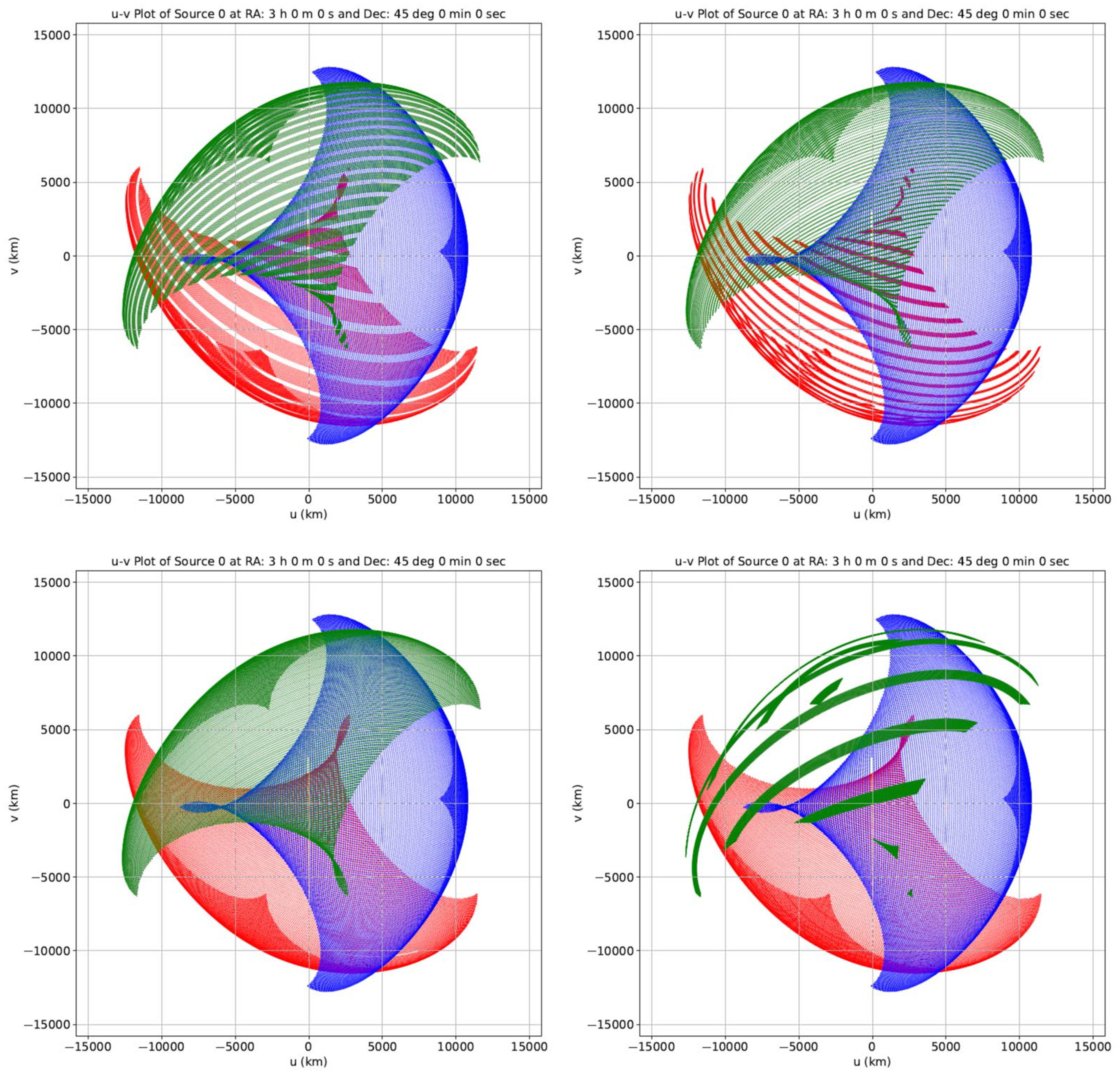
The sensitivity of coverage is also assessed by considering different combinations of the relative initial phases of the satellite orbits. Figure 5 illustrates results of some of these combinations, showing coverage over a duration of 16 days. From among the different combinations of initial orbital phases that were probed, the one in which the satellites 1 has an initial orbital phase of 30 $^{\circ}$
is seen to provide the most uniform and highest density (u,v) coverage.
$^{\circ}$
is seen to provide the most uniform and highest density (u,v) coverage.
The (u,v) coverage obtainable in a 16-day time span for the source direction A is shown, excluding the symmetric counterparts, and the u and v axes are in km. In usual order, the panels show four cases corresponding to the following initial orbital phase for Satellite 1:- 0 $^{\circ}$
, 10
$^{\circ}$
, 10 $^{\circ}$
, 30
$^{\circ}$
, 30 $^{\circ}$
, 45
$^{\circ}$
, 45 $^{\circ}$
|| The significantly higher uniformity in the (u,v) coverage is readily evident for the case with 30
$^{\circ}$
|| The significantly higher uniformity in the (u,v) coverage is readily evident for the case with 30 $^{\circ}$
phase.
$^{\circ}$
phase.
The final values of the orbital parameters (as mentioned in Table 1) were chosen after probing numerous cases of coverage and obtaining the best possible uniformity, and hence the highest possible density, of coverage, attainable over a duration of 16 days, for all the three special source directions.
It is important to emphasise that the duration of 16 days, as a specific time span referred to here and later, is picked merely as an indicating interval over which 85% or greater of the potential maximum coverage that a given baseline offers is obtained. Beyond this time, the approach to the respective maximum coverage is relatively slow. It is also worth remembering that the so-called coverage is assessed in the (u,v) plane which, for simplicity, has a rather coarse grid (100 km) presently (more on this in Subsection 3.2 and the corresponding footnote). Assessment on a finer grid in (u,v) plane would correspondingly stretch the time spans required for similar fractional coverages. However, it is important to note that much of the extent of the potential coverage in (u,v) is spanned in the mentioned duration of about 16 days or even quicker, and the gaps get filled progressively with increasing time.
It should also be emphasised that while some specific combinations of the orbital parameters might appear to provide noticeably better coverage than others, its significance is to be appreciated more in terms of the speed of coverage. When assessed over suitably longer durations, most combinations of orbital parameters relevant to LEO would provide (u,v) coverages that compare well with the best possible for the three-satellite system. Thus, if higher coverage is a priority, then the sources can be observed for a suitably longer duration even if the orbital heights (or periods) and initial orbital phases of the satellites are not optimal.
In general, optimising one parameter at a time sequentially may not yield optimal combination. However, in the present case, the altitude is merely a proxy for the orbital period (or frequency), which dictates the rate of change of orbital phase. Hence, it is not at all surprising that both the altitude and the initial phase have similar effect as they together decide the orbital phase, and hence the location of a given satellite. As a consequence, the baseline vector defined by relative locations for the pair of satellites would also respond to the combination of orbital phases (each in turn depends only on the combination of period and initial phase).
Now we discuss the implications of the fact that, in practice, exact match to a specified orbit, such as in our model, may not be assured. There will, of course, be finite sensitivity to the parameters, including inclination and Right Ascension of the Ascending Node (RAAN). Fortunately, the absolute RAANs or inclinations, and therefore absolute orientations of the orbital axes, are not important in the present astronomy context, as long as the relevant differences ensure mutual orthogonality. With three mutually orthogonal orbits, one indeed ensures that each octant has similar set of coverages. Slight violation of mutual orthogonality of the orbits will be the essential outcome of any moderate non-idealities in the relative orientations of three orbital axes. The pseudo octants in such a case will differ from each other, and hence will the set of associated coverages. The most relevant change in the coverage will be for the outermost baselines. A slightly shrunken pseudo octant will have reduction in the respective baseline lengths, but only by a (rather slowly varying) factor of ( $\cos\frac{\phi}{2} - \sin\frac{\phi}{2}$
), where
$\cos\frac{\phi}{2} - \sin\frac{\phi}{2}$
), where $\phi$
is the reduction (or deviation) in angle from the desired orthogonality. The sources in opposite octant will see increase in corresponding baseline extent by a factor of (
$\phi$
is the reduction (or deviation) in angle from the desired orthogonality. The sources in opposite octant will see increase in corresponding baseline extent by a factor of ( $\cos\frac{\phi}{2} + \sin\frac{\phi}{2}$
). Thus, even a 5
$\cos\frac{\phi}{2} + \sin\frac{\phi}{2}$
). Thus, even a 5 $^{\circ}$
deviation from orthogonality will change the corresponding baseline extent only by less than 5%, much less than the source direction-dependent variation.
$^{\circ}$
deviation from orthogonality will change the corresponding baseline extent only by less than 5%, much less than the source direction-dependent variation.
3.2. Quantitative Assessment of the (u,v) Coverage
Having so far assessed the coverages more qualitatively, we proceed to present indicative quantitative measures of the coverage in the (u,v) plane, for all the three special source directions defined in the beginning of this section.
For this purpose, we need to assert the gridding scheme in the spatial frequency, that is, the (u,v) plane. Ideally, for wide-field imaging configuration, the gridding might need to be as fine as the size of the aperture (in units of wavelength) associated with each of the interferometric elements, or a few times finer than that implied by the inverse of the angular size of the field we wish to image at a time. For convenience in computation, although at the risk of our quantitative results appearing somewhat misleading in their absolute measures, we have chosen to grid the (u,v) plane significantly coarsely. Although the (u,v) cell size can be varied in our simulations, the quantitative results here are based on a cell size of 100 km $\times$
100 km, as mentioned even earlier, which suffices for the relative assessmentFootnote
c
. By considering the cell as filled if one or more (u,v) points fall within that cell, we estimate the so-called sampling function, S(u,v), providing the description of the spatial frequency coverage, and then percentage coverage was calculated by comparing it with the limiting (u,v) span assumed as a circle of radius 15 750 km (maximum baseline length). For completeness, we do include the coverage symmetry in (u,v) plane, resulting from the Hermitian symmetric nature of the visibilities.
$\times$
100 km, as mentioned even earlier, which suffices for the relative assessmentFootnote
c
. By considering the cell as filled if one or more (u,v) points fall within that cell, we estimate the so-called sampling function, S(u,v), providing the description of the spatial frequency coverage, and then percentage coverage was calculated by comparing it with the limiting (u,v) span assumed as a circle of radius 15 750 km (maximum baseline length). For completeness, we do include the coverage symmetry in (u,v) plane, resulting from the Hermitian symmetric nature of the visibilities.
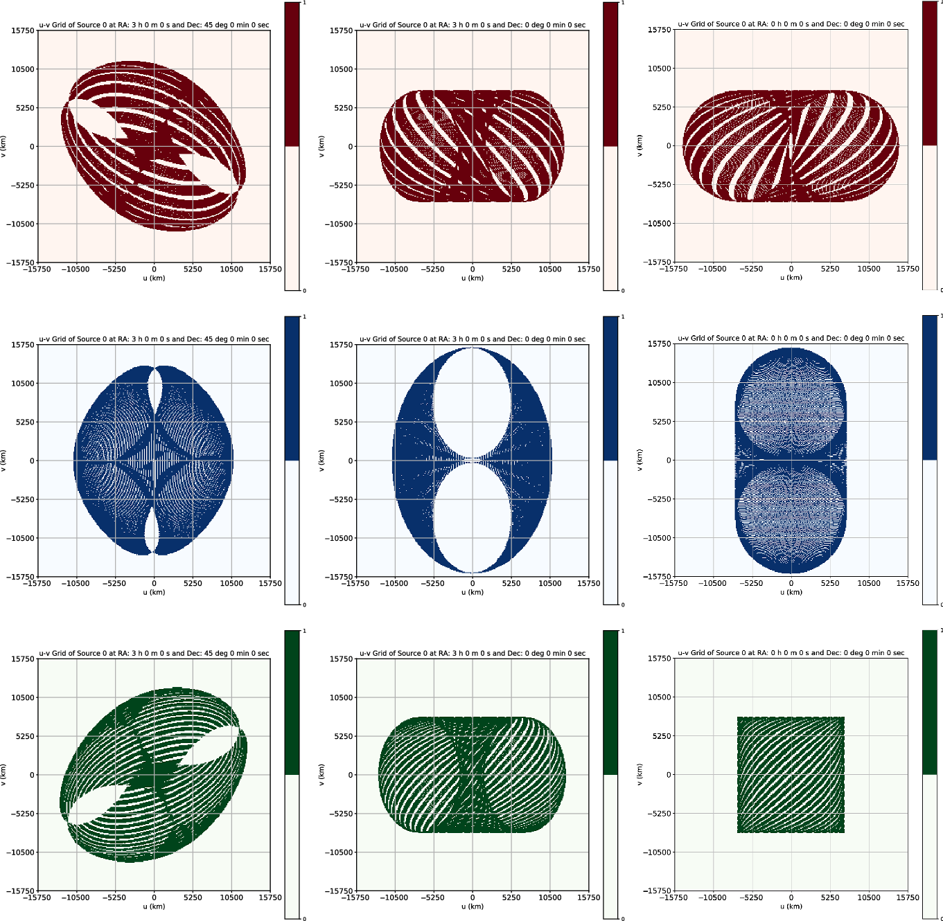
When the source direction A is observed for a duration of 16 days, the percentage coverages from the baseline due to satellite pairs 1–2, 2–3, and 3–1 are about 39.5, 46, and 39.5 %, respectively, with the total coverage being about 64%. Refer to Figure 6 for further details and results.
The coarsely gridded (u,v) coverages using the three-satellite system over a time span of 16 days are shown, with u and v axes marked in km. The three columns correspond to the three special source directions, namely the source A, B, and C, in that order (see main text for the definition of these special directions). The different rows refer to the coverage corresponding to the different baselines, namely 1–2, 2–3, and 3–1, in that order.
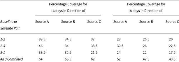
These results (summarised in Table 2) show that the total coverage for any source observed for a time duration of 16 days would, thus, lie between 64% and 55.5%. The table also has results corresponding to observations done for time durations of 8 days for the same three chosen source directions. These values will be referred to in Subsection 3.5. Also, the coverages due to our system are much greater than what we usually get with the ground-based counterparts when compared for the same time duration. This means that while having greater baselines, our model system is also capable of giving significantly better coverage for any source, which would result in very fine angular resolutions at low radio frequencies.
Pair-wise and total (u,v) coverage with 3 satellites for different chosen directions observed for a span of 16 days and 8 days respectively
3.3. Dirty Beams or the Point Spread Functions
The dirty beam, or the point spread function, associated with the total spatial frequency (or (u,v)) coverage obtainable, for each of the three special source directions, is estimated separately, by performing the 2D (Inverse) Fourier transform of the respective (u,v) coverage data.
The dirty beam, b(l, m) is given by:
 \begin{equation} b(l,m) = \mathcal{F}^{-1} [S(u,v)], \end{equation}
where S(u,v) is the sampling function for the visibility measurements, describing the effective coverage in the spatial frequency plane, while the dirty beam is a function of direction defined by l and m, which are the direction cosines of angles in the planes containing u and v, respectively. The sampling function S(u,v) depends on actual (natural) sampling described by s(u,v) and a user-specified weighting function W(u,v), in the following way:
 \begin{equation} S(u,v) = s(u,v)W(u,v). \end{equation}
In our simulation, we have assumed uniform weighting, in which W(u,v) is inversely proportional to the local density of (u,v) points in s(u,v). The sum of weights in a (u,v) cell is constant if the cell is filled and zero if the cell is empty. This implementation ensures that the (u,v) plane is filled more uniformly and the dirty beam side lobes are minimum. Such an implementation enhances angular resolution as it gives more weight to longer baselines, at the expense of point source sensitivity. Since our model system has wide-field antennas with very large baselines, uniform weighing is more appropriate (see for more details, Wilner (Reference Wilner2010)), and is employed in the estimation of the dirty beams shown in Figure 7. It should be noted that the x and y axes of the dirty beam plots are RA offset and Dec offset, respectively, but are not shown in the figures as we have not assumed any spatial frequencies in the (u,v) graphs. For example, when assuming a spatial frequency of 0.3 MHz, the extent of both RA offset and Dec offset in the dirty beam plots would be from about $-3$
arcsec to +3 arcsec. These values can be trivially scaled for any other radio frequency in a similar manner.
$-3$
arcsec to +3 arcsec. These values can be trivially scaled for any other radio frequency in a similar manner.
The top row panels show the combined (u,v) coverage, obtainable using the three-satellite configuration, for the three special source directions (source A, B, and C), and the corresponding dirty beams in the bottom row, assuming uniform weighting.
3.4. Sun Observation
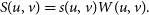
Here, we examine a special case for observation of the Sun using our space interferometer set-up. The Sun, as a source at a finite distance of 1 AU, represents indeed an additional special scenario, as the Earth orbits around it, making its apparent direction (i.e., RA and Dec) change systematically. With appropriate modifications to take these aspects into account, the attainable (u,v) coverage is estimated, assuming time duration of 16 days. The combined percentage coverage in this case is found to be about 63%, reassuringly in the range of coverage noted in Subsection 3.2. Figure 8 shows the relevant details of the (u,v) coverage, over a duration of 16 days, and the corresponding dirty beam.
The total (u,v) coverage plot for the Sun observation for a duration of 16 days and its corresponding dirty beam.
Admittedly, the Sun is a very broad source and more importantly highly variable on a range of timescales, due to a wide variety of reasons. Naturally, therefore, the synthesis imaging combining data over several days in such a case implies a very challenging situation, if not an ill-posed case. However, we have still included this case here merely for completeness, mainly to illustrate the potential (u,v) coverage offered by the proposed configuration.
3.5. Comparison with a Four-Satellite System
Although we have argued and demonstrated that the minimal configuration of three satellites offers largely the desired level of (u,v) coverage, it is important to ask if a four-satellite system would do significantly better. To assess this, we indeed simulated a four-satellite system to examine how much of an advantage adding a fourth satellite would be, how that would be reflected in terms of the improvement in (u,v) coverage and the time taken to obtain desired coverage.
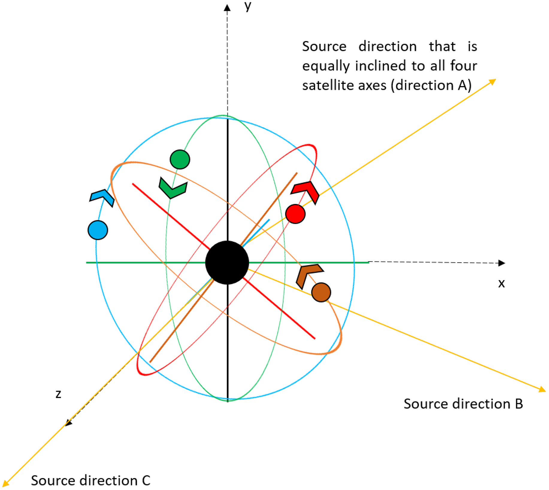
In this modified model, satellites 3 and 4 are in perpendicular polar orbits similar to those of satellites 2 and 3 in the original model (refer to Section 2), while satellites 1 and 2 are in orbits perpendicular to each other with their axes inclined to the Earth’s rotation axis at an angle of 45 $^{\circ}$
and also equally inclined to the axes of satellites 3 and 4, respectively. A simple line diagram in Figure 9 illustrates this four-satellite configuration.
$^{\circ}$
and also equally inclined to the axes of satellites 3 and 4, respectively. A simple line diagram in Figure 9 illustrates this four-satellite configuration.
A line diagram depicting the model with four satellites. The central black sphere represents the Earth, with the red, orange, blue, and green spheres representing the satellites 1, 2, 3, and 4, respectively. Correspondingly, the red, orange, blue, and green axes passing through the Earth’s centre represent the axes of revolution of the satellites 1, 2, 3, and 4, respectively. The yellow rays represent the direction of the sources A, B, and C. The details in the figure are not to scale.
The orbital heights of the satellites above the surface of the Earth are redefined, but the maximum and minimum values are kept the same as those in Table 1. The redefined parameters are given in Table 3. The orbits of all satellites are assumed to be nearly circular and follow the same equations as defined in Section 2. The number of baselines for the four-satellite system is 6 (see Equation (2)). Therefore, this configuration offers twice the number of baselines as that in the three-satellite system.
Defined parameters of the four-satellite model
A special source direction is chosen in such a way that it is equally inclined to all four satellite orbit axes, so as to correspond to the best case, offering maximum (u,v) coverage. This special direction happens to be the same as source direction A (i.e., RA of 3 h and Dec of 45 deg). When a duration of 16 days is considered, as has been standard in the majority of our simulations, the percentage coverages for the source A are 41.5, 23, and 37.5 for the baselines 1–2, 1–3, and 1–4, respectively. The other three baselines, namely 2–3, 2–4, and 3–4, offer percentage coverage of 41.5, 24.5, and 41, respectively. The combined coverage is 61.5%. For the sake of completeness, we also observed for source directions B and C (refer to Section 3) with the four-satellite system. These results are summarised in Table 4.
Pair-wise and total (u,v) coverage with four satellites for different chosen directions observed for a span of 16 days and 8 days, respectively
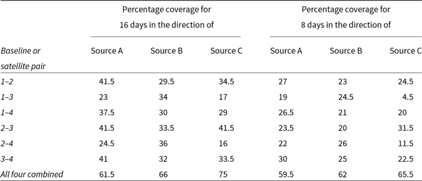
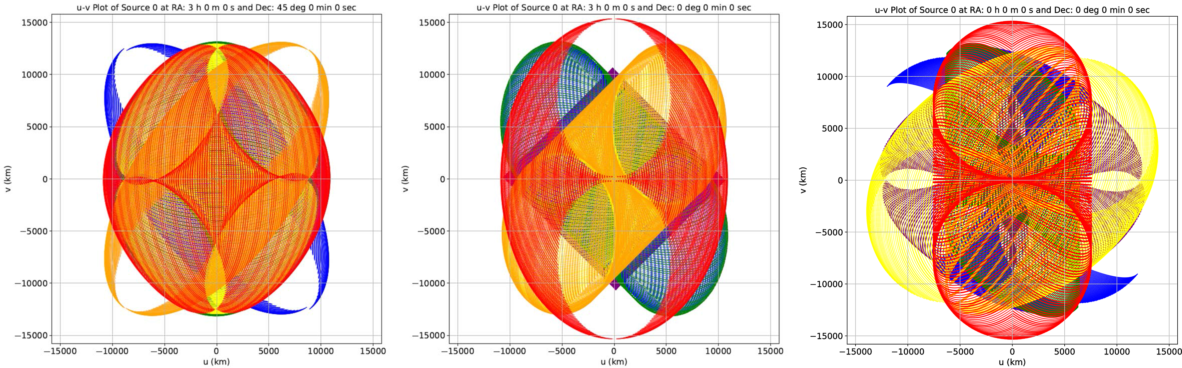
These results indicate that even with a system of four satellites and six baselines, when observing the source A, the total percentage coverage of 61.5% is essentially similar (and slightly lower) to that obtained with three satellites when observed for the same time duration of 16 days. So, when considering the maximum coverage possible, there is no significant improvement even if we employ four satellites. Figure 10 shows the coverage with four satellites for all the three special source directions, assuming a duration of 16 days.
The (u,v) coverages possible with a four-satellite system, over a duration of 16 days, for the source directions A, B, and C, respectively, are shown. The purple, blue, green, yellow, orange, and red tracks correspond to the six baselines formed by satellites 1-2, 1–3, 1–4, 2–3, 2–4, and 3–4, respectively. The u and v axes are marked in km.
However, when we observe the same sources for a duration of 8 days, there is a noticeable improvement in the percentage coverage of the four-satellite system when compared with the three-satellite system for the same duration. The percentage coverages when observing source A corresponding to the individual baselines 1–2, 1–3, 1–4, 2–3, 2–4, and 3–4 are 27, 19, 26.5, 23.5, 22, and 30, respectively, while the combined coverage is about 59.5%. In comparison, the percentage coverage for the same source direction when observed with the three-satellite set-up for 8 days is, 23, 30.5, and 24 for the baselines 1–2, 2–3, and 3–1, respectively, while their combined coverage is close to 52%. The results for all the three source directions in case of three-satellite and four-satellite systems are summarised in Tables 2 and 4, respectively.
These results show that having a four-satellite system can be of great advantage when observing for shorter intervals of time. As already mentioned, when observed for 8 days, the four-satellite system offers an additional 7.5% coverage than that with a three-satellite system, when observing the source A. This difference in coverage increases even more for sources B (by about 14.5%) and C (by about 22%). But if observed long enough, the minimal configuration with just three LEO satellites is seen to be sufficient.
In assessing if any four-satellite system does better, it is important to see if the betterment is significant and commensurate with the fractional increase (of about 30%) in the resource employed. Our choice of orbits in the four-satellite system is prompted by the requirement that coverage, assessed in the three source directions, is as uniform as possible across all octants. Any additional orbit, keeping the three original orbits, will not provide the desired uniformity across octants, even if significant benefits in coverage may be seen in certain directions or octants.
4. Discussion and conclusion
In this last section, we first discuss some of the assumptions and considerations, along with relevant justification and implications.
The encouraging outcome of our present focused exploration, that is, our identification of a novel minimal configuration for apertures in LEO to facilitate high-resolution synthesis imaging at low radio frequencies, paves way to proceed to the next step. This more challenging phase of designing a fuller system, taking into account a range of practical considerations relevant to eventual implementation of this idea, is beyond the scope of present paper. Nonetheless, later in this section, we do allude to some of these aspects relevant to interferometry, such as synchronisation and effect of RFI and briefly discuss the advantages and challenges our minimal configuration implies for operations at low radio frequencies.
In our model, we have assumed the beam of the antenna to be hemispherical with a beam angle of exactly 180 (as shown in Figure 1) but in practice, realising such a beam response for a single element antenna is not possible. Given the science goals of our system, a simple dipole or a tripole antenna would suffice, which however would have a non-uniform directivity. Nevertheless, a suitably arranged array of antenna elements may serve the purpose for catering to the wide-angle coverage.
While estimating the dirty beams, we have employed the uniform weighting function, to maximise angular resolution at the expense of point source sensitivity (e.g., Wilner (Reference Wilner2010)). At such low radio frequencies, the interstellar scattering would be expected to be severe, and the consequent angular broadening (see e.g., Goodman & Narayan (Reference Goodman and Narayan1985), and references therein) should be expected to smoothen the apparent sky brightness distribution by an arcsecond to an arcminute scale, of course depending largely on the frequency and also the sky direction. In such a case, the very high angular resolution offered by our proposed space interferometer would not be as useful, and hence tapering of visibilities at high spatial frequencies might appear more profitable, to reduce the side lobes as well as to improve sensitivity, now at the expense of angular resolution.
While defining the parameters of our model, we assumed only the gravitational pulls due to the Earth and the Sun on the satellites. Although this assumption would be valid for the most part in order to design a practical system, we need to consider all the forces that might affect the motion of the satellite over longer periods. Effects due to the gravitational pulls of the moon and other planets, the precession and nutation of the Earth and the apparent forces acting on the satellites cannot be ignored while considering the evolution of the satellite orbits over very long periods of time.
It is also possible to deliberately use inclined orbits which will precess at a predictable rateFootnote
d
. More specifically, such slightly inclined orbits, for the two presently ideal polar orbits in our model, could be arranged to precess with periods many times the nominal 16-day cycles. A 45 precession of the plane of the orbit about the pole in about 3 months (0.5 $^{\circ}$
/day) would need about 4 to 5 inclination, given the altitudes of our polar orbits (see an early discussion by Searle (Reference Searle1958)). While the inclination will not adversely impact the baselines in any additional manner than due to the effect of non-orthogonality of the orbits (as already assessed/discussed in Subsection 3.1), over the precession cycle, all sources at a given declination will benefit from same coverage, making the total coverage independent of RA (e.g., the coverage for all sources at zero declination will be closely described by a combination of coverages shown for present source directions B and C).
$^{\circ}$
/day) would need about 4 to 5 inclination, given the altitudes of our polar orbits (see an early discussion by Searle (Reference Searle1958)). While the inclination will not adversely impact the baselines in any additional manner than due to the effect of non-orthogonality of the orbits (as already assessed/discussed in Subsection 3.1), over the precession cycle, all sources at a given declination will benefit from same coverage, making the total coverage independent of RA (e.g., the coverage for all sources at zero declination will be closely described by a combination of coverages shown for present source directions B and C).
As can be noted from Stankov et al. (Reference Stankov, Jakowski, Heise, Muhtarov, Kutiev and Warnant2003), the total electron content (TEC) (and thus, the plasma content) of the ionosphere peaks at about 400 km above the surface of the Earth and then drastically falls to a minimum after 700 km. Therefore, in order to avoid the ionospheric plasma and allow the most amount of incident radiation onto our antennas, we chose the orbital heights of the satellites in our model to be well above 700 km. For more details on the attenuation of radio waves due to the ionospheric plasma, see Rao (Reference Rao, Chengalur, Gupta and K. S. Dwarkanath2007).
Intrinsic variability timescales for radio sources, as apparent from flares originating from objects ranging from flare stars to supermassive black holes in AGNs (excluding pulsars and FRBs, but including events like SNe and GRBs), is known to vary from minutes to years (for details see, Pietka et al. (Reference Pietka, Fender and Keane2014)). Variations induced by the effect of intervening medium, such as scintillations, are seen on timescales ranging from seconds to years, the longer timescale being related to refractive effects (see, Goodman & Narayan (Reference Goodman and Narayan1985)).
Each sky direction will be in view of a single aperture (with $\pm 90^{\circ}$
FoV) in LEO for at least half of its orbital period. The considered configuration implies 12–15 orbits in a day for each of the satellites, providing sampling of a comparable number of tracks in the (u,v) plane, per baseline. The revisit time for a given part of sky, as viewed by one of the interferometers, would nominally be half of the longest orbital period (say, an hour), while continuous monitoring is possible over duration of a (u,v) track. If
$\pm 90^{\circ}$
FoV) in LEO for at least half of its orbital period. The considered configuration implies 12–15 orbits in a day for each of the satellites, providing sampling of a comparable number of tracks in the (u,v) plane, per baseline. The revisit time for a given part of sky, as viewed by one of the interferometers, would nominally be half of the longest orbital period (say, an hour), while continuous monitoring is possible over duration of a (u,v) track. If $T_{1}$
and
$T_{1}$
and $T_{2}$
are the orbital periods of two LEO apertures, then the revisits, offering similar set of sampling tracks in (u,v) by the interferometer, are to be expected on timescales decided by the beat between the orbital cycles (i.e.,
$T_{2}$
are the orbital periods of two LEO apertures, then the revisits, offering similar set of sampling tracks in (u,v) by the interferometer, are to be expected on timescales decided by the beat between the orbital cycles (i.e., $(\frac{1}{T_1}-\frac{1}{T_2})^{-1}$
), which in our case, ranges between 0.6 and 1.2 days. Over days, the gaps between the already sampled tracks (extending across the total span) are filled.
$(\frac{1}{T_1}-\frac{1}{T_2})^{-1}$
), which in our case, ranges between 0.6 and 1.2 days. Over days, the gaps between the already sampled tracks (extending across the total span) are filled.
As already mentioned in Subsection 3.1, the 16-day span is merely an indicator of the duration over which a major fraction (over 85%) of the potential sampling in (u,v) plane is attained and does not imply any lower limit for the timescales on which variability can be studied. Although the implicit assumption in synthesis imaging, that the sky distribution is unchanging, is rendered invalid in instances of source variability, the variations themselves are of immense interest to astronomers and any effect of the variability on imaging quality can be desirably mitigated by measuring the variation in adequate detail, and duly accounting for its effect on the image.
Terrestrial man-made RFI continues to be an important and unavoidable issue even in Earth orbits, and more so at low radio frequencies (see Bentum & Boonstra (Reference Bentum and Boonstra2016), and references therein). As already mentioned, our consideration of avoiding ionospheric attenuation of astronomical signals prompts even the closest orbit to be outside the ionosphere. Thus, the severe attenuation of the very low radio frequency signals by the ionosphere, owing to the large electron densities over significant pathlengths, would naturally shield radio sky measurements from contamination due to the terrestrial sources of RFI to certain extent. In addition, our suggested confinement of the FoV implicitly excludes, in principle, any significant antenna response in the directions of the terrestrial sources of RFI, and in practice, any efforts to ensure highly attenuated back lobe responses would not only be desired, but would be richly rewarding. This advantage is not easy to gain for the system using a swarm of satellites, unless such blind-to-Earth mode is explicitly incorporated.
Even if a finite amount of RFI contamination makes its way through the ionosphere to our interferometric elements, on long baselines the individual elements are unlikely to ‘see’ the same sources of RFI (given separated footprints), and hence the picked RFI can be expected to be mutually uncorrelated. Similar argument for uncorrelatedness is applicable to any EMI/RFI from the respective crafts. In instances of contamination from any common source of terrestrial RFI, the large (relative) delays introduced by the ionosphere (particularly at low frequencies and due to the high TEC), as seen on a long baseline, would imply too small decorrelation bandwidths for the RFI to contaminate the visibility measurement in any significant manner. These considerations would be of reducing benefit when the footprints of a pair of satellites overlap, making the paths through the ionosphere less oblique, in addition to seeing the correlated RFI. Hence, the visibility measurements on relatively shorter baselines (<3 000 km) may get affected to the extent that the backlobe response may fail to adequately attenuate signals from the Earth, and their level of surviving phase coherence.
Independent of these considerations, as is widely appreciated, it is essential to ensure that at least the first amplifiers possess high dynamic range, to avoid creation of any intermodulation products, so that at the first opportunity in the following receiver chain it becomes possible to employ suitable spectral filtering, where relevant. As long as RFI is kept to within their respective native bands, suitable detection and excision techniques can be employed in the post-processing (e.g., Deshpande (Reference Deshpande2005)).
On the other side, the ionospheric attenuation in our band would not be as significant as will be for the terrestrial RFI, and hence any RFI from the possible numerous satellites, in the space above our LEO orbits, would be ‘seen’ within the wide FoV of one or more of our satellites. Any formal radio downlink transmission from such satellites would nonetheless be at frequencies much higher than the band of our interest.
However, any out-of-band or spurious signal radiation from other satellites, amounting their lack of electromagnetic compatibility, can potentially contaminate our band of interest. If such RFI is narrow-band, then usual detection and excision procedures, applied separately at each element of our interferometers, would suffice, and the impact can be expected to be limited, in terms of some amount of data loss (usually a small fraction) and corresponding reduction in the system sensitivity. Any broadband RFI from other satellite systems would however need a different strategy, noting the associated challenge and the opportunity. It is easy to see that any broadband RFI from a well-defined direction would be strongly correlated on our baselines, with delay corresponding to relative path difference to our satellites, and these delays would change predictably but distinctly differently from those expected for signals from sky. Thus, sensitive detection of such broadband RFI from each of the other Earth satellites would be possible by identifying and monitoring the associated peaks and their tracks in the dynamic delay spectrum (i.e., Fourier transform of the cross-correlation spectrum). Appropriate filtering based on delay rate would effect desired excision of any significant broadband RFI from such differently moving sources. As an attractive opportunity, such data on the relative delays and their rates of change for all identifiable moving sources of broadband RFI can be used beneficially towards refined monitoring of the changing positions of our satellites, as well as to obtain instructive sampling of delays associated with the upper ionosphere.
The high data rates implied by the proposed wide-band wide-field observations present additional challenges. For our band up to 20 MHz, in dual polarisation, the raw voltage sampling would amount to 80 mega-samples per second, accumulating typically to about 10 GB (for 8-bit samples), at each of our satellites over the duration of respective orbital periods. The downlink channel capacity, thus, needs to be adequately high to transfer $10^{10}$
samples per primary beam or antenna element, from each satellite within a fraction of their respective orbital period whenever ground station access becomes possible. Partial processing performed locally at each satellite, to compute fine resolution spectra and to employ primary detection and excision of any dominant RFI, would help in reducing the dynamic range requirement, and thus, justify any reduction in bit-length per sample, if required. Fortunately, suitable optical/millimeter-wave downlinks can provide attractive bandwidths catering to high rates of data transfers. Similar data exchanges can be considered also between our satellites (e.g., Apoorva et al. (Reference Apoorva, Bitragunta and Nitundil2020), and references therein), which would facilitate on-board computations, including cross-correlation, enabling allowed level of time integration of visibilities to reduce data size, and thus, easing the data rate requirements for the downlinks. While this would facilitate desired immediate local checks on quality of interferometric data, the entire raw voltage data download would remain the preferred mode to enable detailed and sophisticated processing and refinements. In case of stringent constraints from capacity of downlinks, the effective bandwidth to be downloaded can be reduced accordingly, either as a narrower contiguous band or with picket fence sampling across our entire spectral span.
$10^{10}$
samples per primary beam or antenna element, from each satellite within a fraction of their respective orbital period whenever ground station access becomes possible. Partial processing performed locally at each satellite, to compute fine resolution spectra and to employ primary detection and excision of any dominant RFI, would help in reducing the dynamic range requirement, and thus, justify any reduction in bit-length per sample, if required. Fortunately, suitable optical/millimeter-wave downlinks can provide attractive bandwidths catering to high rates of data transfers. Similar data exchanges can be considered also between our satellites (e.g., Apoorva et al. (Reference Apoorva, Bitragunta and Nitundil2020), and references therein), which would facilitate on-board computations, including cross-correlation, enabling allowed level of time integration of visibilities to reduce data size, and thus, easing the data rate requirements for the downlinks. While this would facilitate desired immediate local checks on quality of interferometric data, the entire raw voltage data download would remain the preferred mode to enable detailed and sophisticated processing and refinements. In case of stringent constraints from capacity of downlinks, the effective bandwidth to be downloaded can be reduced accordingly, either as a narrower contiguous band or with picket fence sampling across our entire spectral span.
Two of the most important and integral parts of any interferometry setup are a) the aspect of time synchronisation and b) knowledge of locations of the interferometer elements. Operating at frequencies below 20 MHz relaxes, some of the otherwise demanding requirements encountered at shorter wavelengths. Thus, in our case, a submetre accuracy in positions of phase centres of our apertures would suffice. Similarly, native synchronisation at the level of a few nanoseconds would ensure retention of any coherence intrinsic to the sky signal, while assessing correlation even with the entire bandwidth (say, up to 20 MHz). However, for catering to the wide-field imaging with long baselines, use of fine spectral resolution is essential as already discussed, and hence, the decorrelation delays would be correspondingly large. Even discounting this possible relaxation in time synchronisation requirements, the required accuracies are modest and can be easily met by use of a suitable local frequency reference that has high stability on short term, and phase-locking it to a common standard that has stability on long timescales. In our experience, a Rubidium oscillator disciplined using 1 PPS (one pulse per second) signal from the Global Positioning System (GPS) receiver (see, e.g., Maan et al. (Reference Maan2013)) readily provides the presently required accuracies and is a reliable combination for set-up on-board each of our satellites. A 1 PPS pulse produced by most Rubidium oscillator systems provides a time stamping reference with 1 ns resolution, and a 10-MHz output which forms the reference for phase-locking all local clocks and oscillators. GPS-based orbit determination (see, e.g., Montenbruck (Reference Montenbruck2004)), and verification through calibration observations on bright astronomical sources, will form the basis for estimation of position information with the desired accuracy. A more detailed discussion on these and related aspects, though important, is beyond the scope of the present paper.
To summarise, recognising the need of a fully space-based low-frequency radio observation set-up, we have proposed and studied in detail a minimal configuration of only three apertures, each aboard a LEO satellite, which would be sufficient to map the entire sky, while giving baselines greater than 15 000 km and resolutions finer than 10 arcsec for frequencies under 20 MHz. We have shown that the percentage coverage of this system is also greater than its Earth-based and Earth-and-space-based counterparts and it is able to achieve this in a shorter time span. We have also discussed the special case of the Sun, which does not have fixed RA and Dec. Our assessment of the four-satellite system suggests that adding a fourth satellite would not be of any significant advantage and having just three satellites would be optimum scientifically, technologically, and economically. Although motivated by the requirement of an optimum set-up at low radio frequencies, the various aspects discussed here, including the minimal configuration, are relevant for space interferometry in other wavebands as well.
Acknowledgements
We thank our two anonymous referees for their valuable comments, which have helped towards significant improvement of our manuscript. Akhil Jaini (AJ) would like to thank Raman Research Institute, Bangalore, for providing Visiting Studentship and support to facilitate this study, and Birla Institute of Technology and Science-Pilani, Pilani campus, for providing the opportunity to do this project at the host institute. AJ would also like to thank Hrishikesh Shetgaonkar, Pavan Uttarkar, Pratik Kumar, and Aleena Baby for helpful discussions and insightful comments.