1. Introduction
The Cygnus constellation covers a relevant area of the northern sky and harbours many stellar associations and clusters. The Cygnus OB2 association, at its centre, is a well-studied rich region with several massive stars, as known since the early work of Münch & Morgan (Reference Münch and Morgan1953); Schulte (Reference Schulte1956b,a,1958); Reddish et al. (Reference Reddish, Lawrence and Pratt1966); Knödlseder et al. (Reference Knödlseder, Cerviño, Le Duigou, Meynet, Schaerer and von Ballmoos2002); Albacete Colombo et al. (Reference Albacete Colombo, Caramazza, Flaccomio, Micela and Sciortino2007); see also the review of Reipurth & Schneider (Reference Reipurth and Schneider2008). Recent radio results at arcsecond resolution were presented in Benaglia et al. (Reference Benaglia, Ishwara-Chandra, Intema, Colazo and Gaikwad2020b), further including Cyg OB8 and OB9, using Giant Metrewave Radio Telescope (GMRT) data. Some massive stars towards these regions show significant radio emission, like the Wolf–Rayet stars WR 146, 147, for instance, with their colliding winds, which generate non-thermal (NT) radio fluxes (e.g., Williams et al., Reference Williams, Dougherty, Davis, van der Hucht, Bode and Setia Gunawan1997; Benaglia et al., Reference Benaglia, De Becker, Ishwara-Chandra, Intema and Isequilla2020a, and many references therein). Besides massive, early-type stars, other types of objects were studied in this region like the protoplanetary disk-like sources (Isequilla et al., Reference Isequilla, Fernández-López, Benaglia, Ishwara-Chandra and del Palacio2019) and young stellar objects (YSO, Isequilla et al., Reference Isequilla, Benaglia, Ishwara-Chandra and Intema2020). Some types of Galactic sources, related to stellar systems at different stages, present jet/outflows morphology. Interesting examples are those related to protostars, YSO, and Herbig–Haro objects (HH, see Anglada et al., Reference Anglada, Rodríguez and Carrasco-González2018, the latest review). In the case of HH80/81 and jets, besides NT spectral indices as in other cases, Carrasco-González et al. (Reference Carrasco-González, Rodrgíuez, Anglada, Martí, Torrelles and Osorio2010) measured important linear polarisation, confirming synchrotron emission. We inspect the GMRT images used by Benaglia et al. (Reference Benaglia, Ishwara-Chandra, Intema, Colazo and Gaikwad2020b) to build their catalogue. We identified several faint radio sources with double-lobed mophologies; many of them observed for the first time. And, even though they are towards the Galactic plane, some of them might have an extragalactic nature.
Regular members of the extragalactic zoo, the Active Galactic Nuclei (AGN) are notably strong sources with a spectral energy distribution (SED) ranging from gamma to radio wavelengths (Brown et al., Reference Brown, Duncan, Landt, Kirk, Ricci, Kamraj, Salvato and Ananna2019); generally, the SED presents a peak at UV and significant luminosity contribution at the infrared and X-rays wavelengths. Radio galaxies are a subclass of AGNs. The radio continuum maps usually reveal a bright centre (core), jets, and lobes whose extension can reach Mpc. The radio galaxies were classified into two main kinds, the Fanaroff-Riley I and II (FRI, FRII, Fanaroff & Riley, Reference Fanaroff and Riley1974). The FRIs present their low brightness regions further from the core than their high brightness regions, while it is in the other way round for the FRIIs. At the FRII high brightness regions, the jets are decelerated by the interaction with the circumgalactic medium. Both classic examples are M84 and 3C175, respectively (e.g., Laing et al., Reference Laing, Riley and Longair1983). But the classifications account for the standard type of radio galaxies. Many others with different morphologies, such us X shapes (Leahy & Williams, Reference Leahy and Williams1984), collimated jets, and also some of them with inner double-lobed radio structure as well as a larger outer double-lobed structure, called ‘double-double’ radio galaxies (DDRGs) (Schoenmakers et al., Reference Schoenmakers, de Bruyn, Röttgering, van der Laan and Kaiser2000; Brocksopp et al., Reference Brocksopp, Kaiser, Schoenmakers and de Bruyn2011), were also reported. In addition, the majority of the studies were performed out of the Galactic plane. The optical identification is difficult against a region crowded with emitters at that spectral range, and the lack of high resolution and deep radio images are a problem as well.
An investigation of double-lobed radio sources in the Cygnus region was lacking. In this work, we present the study of the double-lobed type sources in the central part of the Cygnus region, near the Galactic plane, to characterise those with extragalactic features; many of them are reported for the first time in this work. GMRT observations are introduced in Section 2. Section 3 describes the identification processes, and Section 4 the search for counterparts. The discussion is presented in Section 5, and the main conclusions are listed in Section 6.
2. Radio observations
Along the past years, different radio surveys were focused on the Galactic plane and thus on the Cygnus area. Jones et al. (Reference Jones, Garwood and Dickey1988) using the Very Large Array (VLA) carried out continuum observations at 1.4 GHz (
 $b=0^\circ$
). The resolution achieved in this survey was up to 4
$b=0^\circ$
). The resolution achieved in this survey was up to 4
 $^{\prime\prime}$
and the findings complete to about 30 mJy peak in flux density. The results were complemented by Zoonematkermani et al. (Reference Zoonematkermani, Helfand, Becker, White and Perley1990), for
$^{\prime\prime}$
and the findings complete to about 30 mJy peak in flux density. The results were complemented by Zoonematkermani et al. (Reference Zoonematkermani, Helfand, Becker, White and Perley1990), for
 $|b|<0.8^\circ$
, with similar angular resolution and flux limit. In 1996, with the Texas Interferometer at 365 MHz, Douglas et al. (Reference Douglas, Bash, Bozyan, Torrence and Wolfe1996a) imaged the area at arcminutes scale above flux densities of
$|b|<0.8^\circ$
, with similar angular resolution and flux limit. In 1996, with the Texas Interferometer at 365 MHz, Douglas et al. (Reference Douglas, Bash, Bozyan, Torrence and Wolfe1996a) imaged the area at arcminutes scale above flux densities of
 $0.25-0.4\,\mathrm{Jy}$
; and Taylor et al. (Reference Taylor, Goss, Coleman, van Leeuwen and Wallace1996) carried out Westerbork Synthesis Radio Telescope (WSRT) observations at 327 MHz for
$0.25-0.4\,\mathrm{Jy}$
; and Taylor et al. (Reference Taylor, Goss, Coleman, van Leeuwen and Wallace1996) carried out Westerbork Synthesis Radio Telescope (WSRT) observations at 327 MHz for
 $|b|<1.6^\circ$
(WSRT Galactic Plane survey or WSRTGP), achieving an angular resolution of
$|b|<1.6^\circ$
(WSRT Galactic Plane survey or WSRTGP), achieving an angular resolution of
 $\sim1'$
and detecting sources brighter than
$\sim1'$
and detecting sources brighter than
 $10\,\mathrm{mJy\,beam}^{-1}$
. This same interferometer was used to observe the Cyg OB2 region and build the 325 and 1 400 MHz continuum survey, published by Setia Gunawan et al. (Reference Setia Gunawan, de Bruyn, van der Hucht and Williams2003). The attained angular resolutions were 13
$10\,\mathrm{mJy\,beam}^{-1}$
. This same interferometer was used to observe the Cyg OB2 region and build the 325 and 1 400 MHz continuum survey, published by Setia Gunawan et al. (Reference Setia Gunawan, de Bruyn, van der Hucht and Williams2003). The attained angular resolutions were 13
 $^{\prime\prime}$
and 55
$^{\prime\prime}$
and 55
 $^{\prime\prime}$
with
$^{\prime\prime}$
with
 $5\sigma$
flux density limits of
$5\sigma$
flux density limits of
 ${\sim}2\,\mathrm{mJy}$
and
${\sim}2\,\mathrm{mJy}$
and
 $10-15\,\mathrm{mJy}$
, respectively. Very recently, Morford et al. (Reference Morford2020) published results of a deep field mapping of the Cyg OB2 association at 21 cm, attaining an angular resolution of 180 mas and rms as low as 21
$10-15\,\mathrm{mJy}$
, respectively. Very recently, Morford et al. (Reference Morford2020) published results of a deep field mapping of the Cyg OB2 association at 21 cm, attaining an angular resolution of 180 mas and rms as low as 21
 $\mu$
Jy.
$\mu$
Jy.
In order to achieve both high-angular resolution and sensitivity below the mJy threshold, the central
 $19.7\,\mathrm{deg}^2$
of the Cygnus constellation (see Figure 1) were observed using two bands, centred at 325 and 610 MHz, with the Giant Metrewave Radio Telescope. The data were collected during 172 h along 2013–2017, using a 32 MHz bandwidth, and were calibrated and processed uniformly, using the SPAM routines (Intema, Reference Intema2014). For full details on observations, calibration and imaging, see Benaglia et al. (Reference Benaglia, Ishwara-Chandra, Intema, Colazo and Gaikwad2020b). The SPAM routines provided also the final mosaics, one at each band, for which a robust weighting of
$19.7\,\mathrm{deg}^2$
of the Cygnus constellation (see Figure 1) were observed using two bands, centred at 325 and 610 MHz, with the Giant Metrewave Radio Telescope. The data were collected during 172 h along 2013–2017, using a 32 MHz bandwidth, and were calibrated and processed uniformly, using the SPAM routines (Intema, Reference Intema2014). For full details on observations, calibration and imaging, see Benaglia et al. (Reference Benaglia, Ishwara-Chandra, Intema, Colazo and Gaikwad2020b). The SPAM routines provided also the final mosaics, one at each band, for which a robust weighting of
 $-1$
was chosen. We have made use here of the images that are based on those observations. The mosaics present a mean rms of
$-1$
was chosen. We have made use here of the images that are based on those observations. The mosaics present a mean rms of
 $0.5\,\mathrm{mJy\,beam}^{-1}$
and
$0.5\,\mathrm{mJy\,beam}^{-1}$
and
 $0.2\ \mathrm{mJy\,beam}^{-1}$
at 325 and 610 MHz, but we note that the rms value locally varies depending on the presence of extended and/or diffuse emission, up to 0.9 and
$0.2\ \mathrm{mJy\,beam}^{-1}$
at 325 and 610 MHz, but we note that the rms value locally varies depending on the presence of extended and/or diffuse emission, up to 0.9 and
 $0.5\,\mathrm{mJy\,beam}^{-1}$
. The resultant synthesised beams at each frequency at full resolution were
$0.5\,\mathrm{mJy\,beam}^{-1}$
. The resultant synthesised beams at each frequency at full resolution were
 $10'' \times 10''$
, and
$10'' \times 10''$
, and
 $6'' \times 6''$
. The final mosaic image sizes resulted in (
$6'' \times 6''$
. The final mosaic image sizes resulted in (
 $6\,487 \times 6\,573$
), and (
$6\,487 \times 6\,573$
), and (
 $12\,580 \times 13\,837$
) pixels, of sizes
$12\,580 \times 13\,837$
) pixels, of sizes
 $2.5''$
and
$2.5''$
and
 $1.5''$
, respectively. We note that this paper is the fourth of a series derived from the analysis of the Cygnus region through GMRT observations, see Benaglia et al. (Reference Benaglia, De Becker, Ishwara-Chandra, Intema and Isequilla2020a,b, Reference Benaglia, Ishwara-Chandra, Paredes, Intema, Colazo and Isequilla2021). Besides the SPAM mosaics, we used, for some specific regions, complementary images built with the astronomical image processing system (AIPS, Greisen, Reference Greisen2003), following standard procedures, and different weightings (see Benaglia et al., Reference Benaglia, Ishwara-Chandra, Paredes, Intema, Colazo and Isequilla2021, for details).
$1.5''$
, respectively. We note that this paper is the fourth of a series derived from the analysis of the Cygnus region through GMRT observations, see Benaglia et al. (Reference Benaglia, De Becker, Ishwara-Chandra, Intema and Isequilla2020a,b, Reference Benaglia, Ishwara-Chandra, Paredes, Intema, Colazo and Isequilla2021). Besides the SPAM mosaics, we used, for some specific regions, complementary images built with the astronomical image processing system (AIPS, Greisen, Reference Greisen2003), following standard procedures, and different weightings (see Benaglia et al., Reference Benaglia, Ishwara-Chandra, Paredes, Intema, Colazo and Isequilla2021, for details).
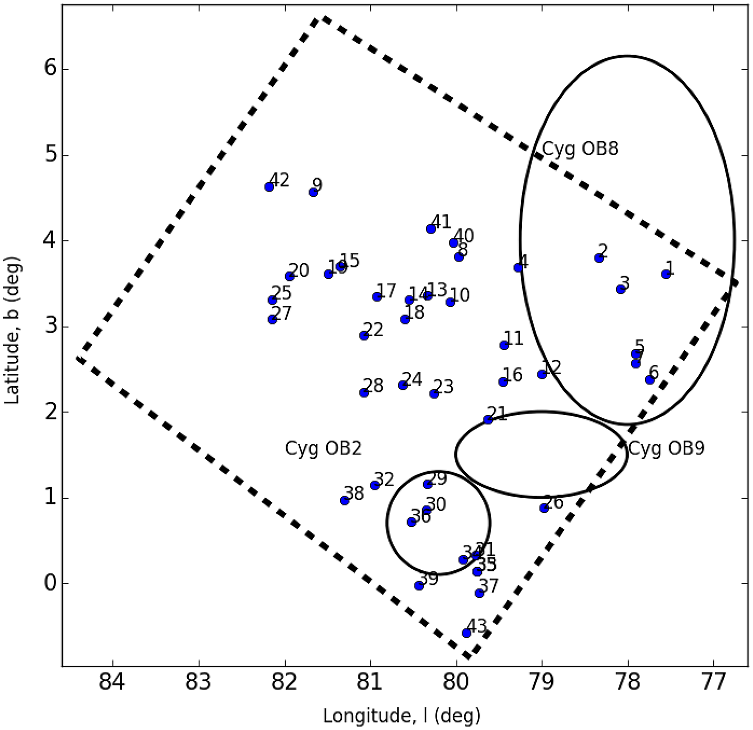
Observed area of the Cygnus constellation marked with a black dashed contour box, over the identified stellar associations Cygnus OB2 and Cygnus OB8 as well as Cygnus OB9. The blue dots are the double-lobed sources presented in this paper, with ID numbers as in Table 1.
3. Identifying double-lobed sources in the cygnus region
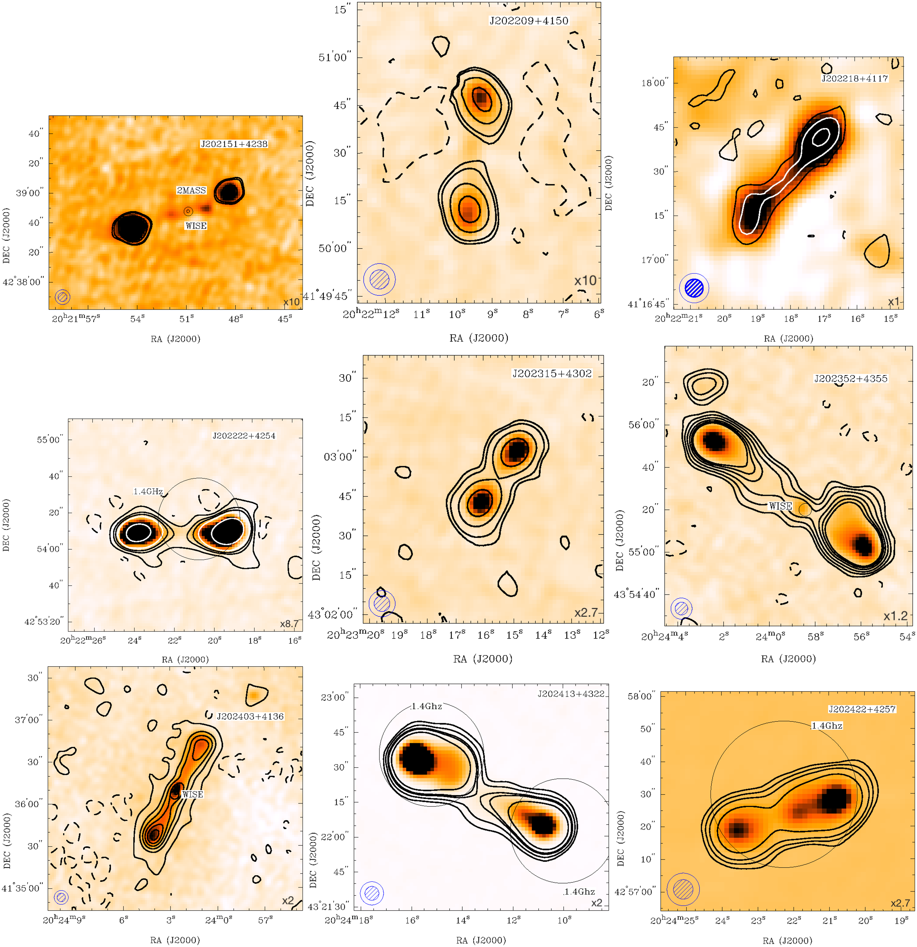
For the present study, we visually searched in the image mosaics for objects with two bright peaks, within a few arcminutes apart, joined by a bridge or path of emission, either diffuse or intense, or with a central nucleus. We proposed them as ‘double-lobed’ candidatesFootnote a. To take into consideration the diverse local rms, we made individual images of each source, showing simultaneously the continuum emission at both bands when possible, see Figures A1, A2, A3, A4, A5, and A6.
The spectral index (
 $\alpha$
) of a source is a key parameter to reveal its nature. It is defined in terms of the integrated flux density S at frequency
$\alpha$
) of a source is a key parameter to reveal its nature. It is defined in terms of the integrated flux density S at frequency
 $\nu$
; here we used the convention
$\nu$
; here we used the convention
 $S_{\nu} \propto \nu^\alpha$
. To build the spectral index map of sources, we convolved and regridded the 610 MHz image to exactly the same synthesised beam and grid as the 325 MHz one (thus the pixel size in both maps is the same,
$S_{\nu} \propto \nu^\alpha$
. To build the spectral index map of sources, we convolved and regridded the 610 MHz image to exactly the same synthesised beam and grid as the 325 MHz one (thus the pixel size in both maps is the same,
 $2.5''\times2.5''$
). The miriad task cgcurs was used to estimate the integrated flux densities of the identified sources, within the region defined by 3 times the local rms. The main radio properties of the identified double-lobed sources are listed in Table 1, being
$2.5''\times2.5''$
). The miriad task cgcurs was used to estimate the integrated flux densities of the identified sources, within the region defined by 3 times the local rms. The main radio properties of the identified double-lobed sources are listed in Table 1, being
Position, integrated flux density and spectral index of double-lobed sources components, and total spectral index. Nu: nucleus, G: geometric centre, B: bridge.
 $SC_{610\,{\rm MHz}}$
refers to the integrated flux density obtained from the 610 MHz image convolved to the 325 MHz beam.
$SC_{610\,{\rm MHz}}$
refers to the integrated flux density obtained from the 610 MHz image convolved to the 325 MHz beam.
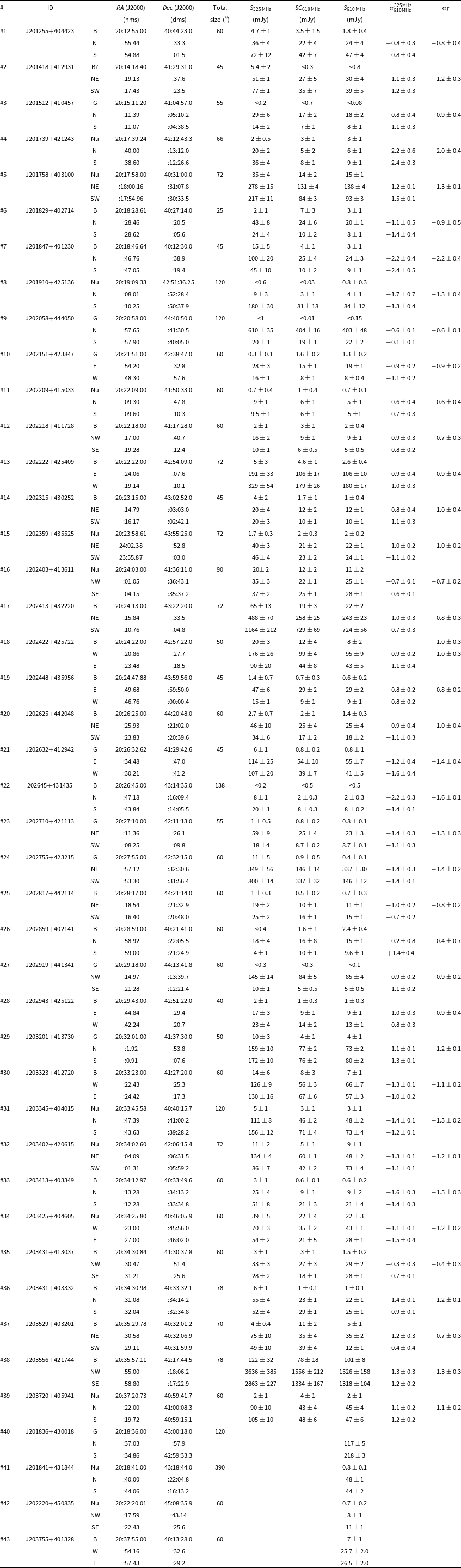
Column (1)—Source/candidate number (#).
Column (2)—Source ID. The sources are listed in increasing order of right ascension: first those with GMRT data at both bands, and second the ones with only 610 MHz data.
Column (3)—Label corresponding to the type of source centre, as (B): detected bridge; (Nu): detected nucleus candidate; (G) measured geometric centre. The orientation of the lobes is quoted by means of cardinal celestial points (N, S, E, W, NW, SE, NE, and SW).
Columns (4,5)—J2000 position in right ascension and declination of the components identified in Column 3.
Columns (6)—The total extension of the sources derived considering the distance between the extreme of the outermost contour (=3 rms) of each lobe at 325 MHz. Estimated errors:
 $\pm 2\,\mathrm{arcsec}$
.
$\pm 2\,\mathrm{arcsec}$
.
Columns (7)–(9)—Integrated flux density of each component, at the 325 MHz image, at the 610 MHz image convolved to the 325 MHz beam, and at the 610 MHz full resolution image, respectively. The error corresponds to
 $3 \sigma$
(with
$3 \sigma$
(with
 $\sigma$
, local rms). When a source was detected at one frequency only, the upper limit—at the other frequency band—corresponds to three times the local rms noise. Whenever was possible to calculate the integrated flux density of the bridge emission, we measured its flux above
$\sigma$
, local rms). When a source was detected at one frequency only, the upper limit—at the other frequency band—corresponds to three times the local rms noise. Whenever was possible to calculate the integrated flux density of the bridge emission, we measured its flux above
 $3 \sigma$
, checking not to introduce the emission from the lobes. Since all nuclei sizes were encompassed by one beam, their integrated flux densities were calculated over the beam size area.
$3 \sigma$
, checking not to introduce the emission from the lobes. Since all nuclei sizes were encompassed by one beam, their integrated flux densities were calculated over the beam size area.
Column (10)—Spectral index
 $\alpha$
of the component identified in Column 3.
$\alpha$
of the component identified in Column 3.
Column (11)—Total spectral index
 $\alpha_T$
of the double-lobed source candidate; calculated using the flux sum of each source component.
$\alpha_T$
of the double-lobed source candidate; calculated using the flux sum of each source component.
4. Multi-wavelength cross-identification and analysis
Once we have identified and characterised the position and the integrated flux density of the double-lobed source candidates in the radio images, we made use of NEDFootnote b and SIMBADFootnote c databases to perform multi-wavelength cross-match positional association at other frequencies. For every double-lobed source, we defined three search regions: one for each lobe and a third for its central point/source/bridge. We consulted the specific catalogues to gather additional information if necessary. In the following subsections, we describe the results.
4.1. Radio sources
We found radio counterparts for many of the double-lobed sources candidates. In most cases, the matches belong to the NRAO VLA Sky Survey (NVSS, Condon et al., Reference Condon, Cotton, Greisen, Yin, Perley, Taylor and Broderick1998), performed with the Very Large Array (VLA) at 1.4 GHz, with an angular resolution of 45
 $^{\prime\prime}$
. Furthermore, many others were reported in surveys carried out with the WSRT, such as the ones mentioned in Section 2 by Taylor et al. (Reference Taylor, Goss, Coleman, van Leeuwen and Wallace1996) and by Setia Gunawan et al. (Reference Setia Gunawan, de Bruyn, van der Hucht and Williams2003). To highlight the information at 1 400 MHz and emphasise the improvement of the angular resolution at 325 MHz that our observations reached, we present, in Figures A1–A6, the counterparts found corresponding to the NVSS and WSRT surveys with circles of the size of their attained beams and labelled as ‘1.4 GHz’ and ‘327 MHz’, respectively. Additional detection, reported by previous studies, were also found (but not shown, for the sake of clarity). We will mention them as we describe the counterparts found for each source. For all double-lobed sources with NVSS counterparts, we gathered the NVSS integrated flux density at 1.4 GHz, and, using the convolved maps (to a 45
$^{\prime\prime}$
. Furthermore, many others were reported in surveys carried out with the WSRT, such as the ones mentioned in Section 2 by Taylor et al. (Reference Taylor, Goss, Coleman, van Leeuwen and Wallace1996) and by Setia Gunawan et al. (Reference Setia Gunawan, de Bruyn, van der Hucht and Williams2003). To highlight the information at 1 400 MHz and emphasise the improvement of the angular resolution at 325 MHz that our observations reached, we present, in Figures A1–A6, the counterparts found corresponding to the NVSS and WSRT surveys with circles of the size of their attained beams and labelled as ‘1.4 GHz’ and ‘327 MHz’, respectively. Additional detection, reported by previous studies, were also found (but not shown, for the sake of clarity). We will mention them as we describe the counterparts found for each source. For all double-lobed sources with NVSS counterparts, we gathered the NVSS integrated flux density at 1.4 GHz, and, using the convolved maps (to a 45
 $^{\prime\prime}$
beam) at 610 MHz, we derived the spectral index. The results are shown in Table 2.
$^{\prime\prime}$
beam) at 610 MHz, we derived the spectral index. The results are shown in Table 2.
Integrated flux density of NVSS counterparts, and spectral indices.
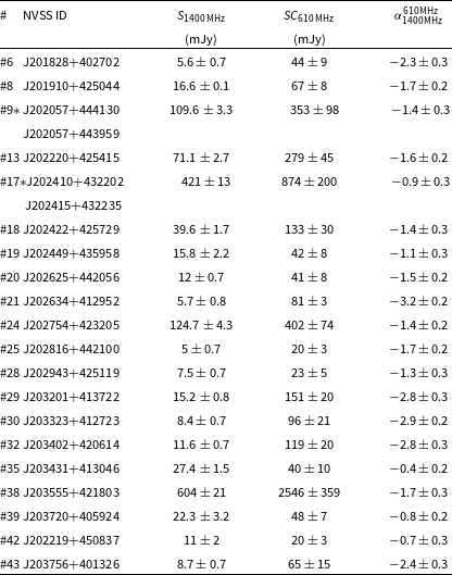
The spectral indices were derived between catalogued NVSS integrated flux densities (S) and the convolved integrated flux densities (SC) of the double-lobed sources at 610 MHz. *In order to estimate the total spectral index, we added the NVSS integrated flux densities of both lobes.
The spectral index plays an important role in the identification of the dominating process leading to the observed emission. It is well known that negative spectral index values in radio are indicative of a non-thermal emission origin, related to extragalactic sources (e.g., synchrotron, Ginzburg & Syrovatskii, Reference Ginzburg and Syrovatskii1967), but setting a limit is not straight forward around zero values (
 $0.5<\alpha<-0.5$
) because this range is indicative of optically thin free–free emission (from star-forming galaxies or Galactic ionised objects for instance), and also of thick synchrotron emission (core-dominated AGNs). Positive spectral index values can be associated with young compact sources (e.g., Saikia et al., Reference Saikia, Thomasson, Roy, Pedlar and Muxlow2004; Pratap & McIntosh, Reference Pratap and McIntosh2005).
$0.5<\alpha<-0.5$
) because this range is indicative of optically thin free–free emission (from star-forming galaxies or Galactic ionised objects for instance), and also of thick synchrotron emission (core-dominated AGNs). Positive spectral index values can be associated with young compact sources (e.g., Saikia et al., Reference Saikia, Thomasson, Roy, Pedlar and Muxlow2004; Pratap & McIntosh, Reference Pratap and McIntosh2005).
Since our celestial region of study is nearby the Galactic plane, to be conservative, we considered a limiting spectral index value of
 $-0.7$
as the main criterion to discriminate the double-lobed source candidates between extragalactic (
$-0.7$
as the main criterion to discriminate the double-lobed source candidates between extragalactic (
 $\alpha \leq -0.7$
) or Galactic (
$\alpha \leq -0.7$
) or Galactic (
 $\alpha > -0.7$
) origin (see, for instance, Ibar et al., Reference Ibar, Ivison, Best, Coppin, Pope, Smail and Dunlop2010; Ocran et al., Reference Ocran, Taylor, Vaccari, Ishwara-Chandra and Prandoni2020). Whenever was possible, we did also consider the value of the spectral index
$\alpha > -0.7$
) origin (see, for instance, Ibar et al., Reference Ibar, Ivison, Best, Coppin, Pope, Smail and Dunlop2010; Ocran et al., Reference Ocran, Taylor, Vaccari, Ishwara-Chandra and Prandoni2020). Whenever was possible, we did also consider the value of the spectral index
 $\alpha_{1400\,\rm MHz}^{610\,\rm MHz}$
in our classification. The detailed information of the flux densities measured and the spectral indices derived are given in Tables 1
$\alpha_{1400\,\rm MHz}^{610\,\rm MHz}$
in our classification. The detailed information of the flux densities measured and the spectral indices derived are given in Tables 1
 $\&$
2.
$\&$
2.
4.2. Sources at other wavelengths
Although NED and SIMBAD databases cover the entire electromagnetic spectrum, besides radio sources, only infrared ones were found, except for one X-ray counterpart. Infrared sources are expected to be frequent in the line of sight towards the Cygnus region. But we note that as double radio sources are likely extragalactic objects, and the Cygnus OB2 region is in the Galactic plane, it is remarkably challenging to find conclusive evidence of the right counterparts in optical/IR for these radio sources.
Even though we defined three search regions, as is explained at the beginning of the section, we focused the infrared search on the surroundings of the centre (Nu) or the geometric centre (G) of the double-lobed sources, considering that we aim to identify the possible host galaxy for the proposed extragalactic sources. In checking for the positional overlapping in the plane of the sky, we considered the following extensions of infrared sources for each catalogue using circles with diameters of: 6
 $^{\prime\prime}$
for WISE (Wright et al., Reference Wright2010), 2
$^{\prime\prime}$
for WISE (Wright et al., Reference Wright2010), 2
 $^{\prime\prime}$
for 2MASS (Skrutskie et al., Reference Skrutskie2006), 2
$^{\prime\prime}$
for 2MASS (Skrutskie et al., Reference Skrutskie2006), 2
 $^{\prime\prime}$
for Spitzer (Werner et al., Reference Werner2004), and 18
$^{\prime\prime}$
for Spitzer (Werner et al., Reference Werner2004), and 18
 $^{\prime\prime}$
for IRAS (Neugebauer et al., Reference Neugebauer1984). Below, we present fully the arguments that led us to the classification of each double-lobed source.
$^{\prime\prime}$
for IRAS (Neugebauer et al., Reference Neugebauer1984). Below, we present fully the arguments that led us to the classification of each double-lobed source.
4.3. Extragalactic sources
J201255+404423 (#1), J201418+412931 (#2), and J201847+401230 (#7). At the position of these sources there are no detection at other frequencies, see Figure A1. An inclination of the line linking the lobes towards the line of sight, will result in a modification of the actual sizes/shapes as seen in the images. In particular, an inclination angle smaller than 45 deg will imply higher projection effects, including the appreciation of lobes with different sizes. We interpret that this is the case for source #1.
J201739+421243 (#4) and J201758+403100 (#5). For these sources we found no associations at other frequencies, see Figure A1. As a complement, we show the spectral index maps as well as the error distribution in Figure B1.
J201829+402714 (#6) and J201910+425136 (#8). Both sources have positional coincidences with NVSS catalogued records, see Table 2. For #8, the NVSS component overlaps only the southern lobe (NVSS ID: J201910+425044). The radio counterpart of #6, which is a component of the NVSS survey is not resolved, see Figure A1.
J202151+423847 (#10). There are two possible associations at infrared wavelengths for this source: WISEA J202150.84
 $+$
423846.9 and 2MASS J20215131
$+$
423846.9 and 2MASS J20215131
 $+$
4238521, coincident with the position of the geometric centre. Besides, the radio image at 610 MHz reveals two knots in between the IR sources and the lobes (see Figures A2 and C1). These knots could be part of common bipolar jets (an unseen weak bridge) formed time ago, of an AGN with much activity in the past. The morphology could be also indicative of DDRG, as two double radio galaxies that share a centre.
$+$
4238521, coincident with the position of the geometric centre. Besides, the radio image at 610 MHz reveals two knots in between the IR sources and the lobes (see Figures A2 and C1). These knots could be part of common bipolar jets (an unseen weak bridge) formed time ago, of an AGN with much activity in the past. The morphology could be also indicative of DDRG, as two double radio galaxies that share a centre.
J202209+415033 (#11), J202218+411728 (#12), J202222+425409 (#13), and J202315+430252 (#14). For these sources, there are no detection at other wavelengths, except for #13, which has one radio counterpart, unresolved, at 1.4 GHz, see Figure A2 and Table 2.
J202359+435525 (#15). There is one possible association at infrared wavelengths (WISEA J202358.42
 $+$
435519.3), in agreement with the position of the nucleus, see Figures A2 and C1. It might be revealing the location of the putative host galaxy. We show the spectral index distribution and error maps; see Figure B1.
$+$
435519.3), in agreement with the position of the nucleus, see Figures A2 and C1. It might be revealing the location of the putative host galaxy. We show the spectral index distribution and error maps; see Figure B1.
J202403
 $+$
413611 (#16). For this object, there is one possible association at infrared frequencies (WISEA J202403.03+413611.3), at its geometric centre; see Figures A2 and C1. Considering the spectral index value within the errors, the object might be an extra-galactic source where the core may have reignited, giving it a similar brightness as the southern lobe.
$+$
413611 (#16). For this object, there is one possible association at infrared frequencies (WISEA J202403.03+413611.3), at its geometric centre; see Figures A2 and C1. Considering the spectral index value within the errors, the object might be an extra-galactic source where the core may have reignited, giving it a similar brightness as the southern lobe.
J202413+432220 (#17). This source was detected by previous radio surveys: at 365 MHz with the TEXAS telescope (Douglas et al., Reference Douglas, Bash, Bozyan, Torrence and Wolfe1996b,
 $\textit{S} = 1.76\pm0.14\,\mathrm{Jy}, 4'$
beam), and at 5 GHz with the MIT-green Bank telescope (Bennett et al., Reference Bennett, Lawrence, Burke, Hewitt and Mahoney1986,
$\textit{S} = 1.76\pm0.14\,\mathrm{Jy}, 4'$
beam), and at 5 GHz with the MIT-green Bank telescope (Bennett et al., Reference Bennett, Lawrence, Burke, Hewitt and Mahoney1986,
 $\textit{S} = 69\pm 11\,\mathrm{mJy}$
, beam of 3
$\textit{S} = 69\pm 11\,\mathrm{mJy}$
, beam of 3
 $^{\prime}$
). We found two NVSS components coincident with each lobe (NVSS IDs: J202410+432202, J202415+432235); see Figure A2 and Table 2.
$^{\prime}$
). We found two NVSS components coincident with each lobe (NVSS IDs: J202410+432202, J202415+432235); see Figure A2 and Table 2.
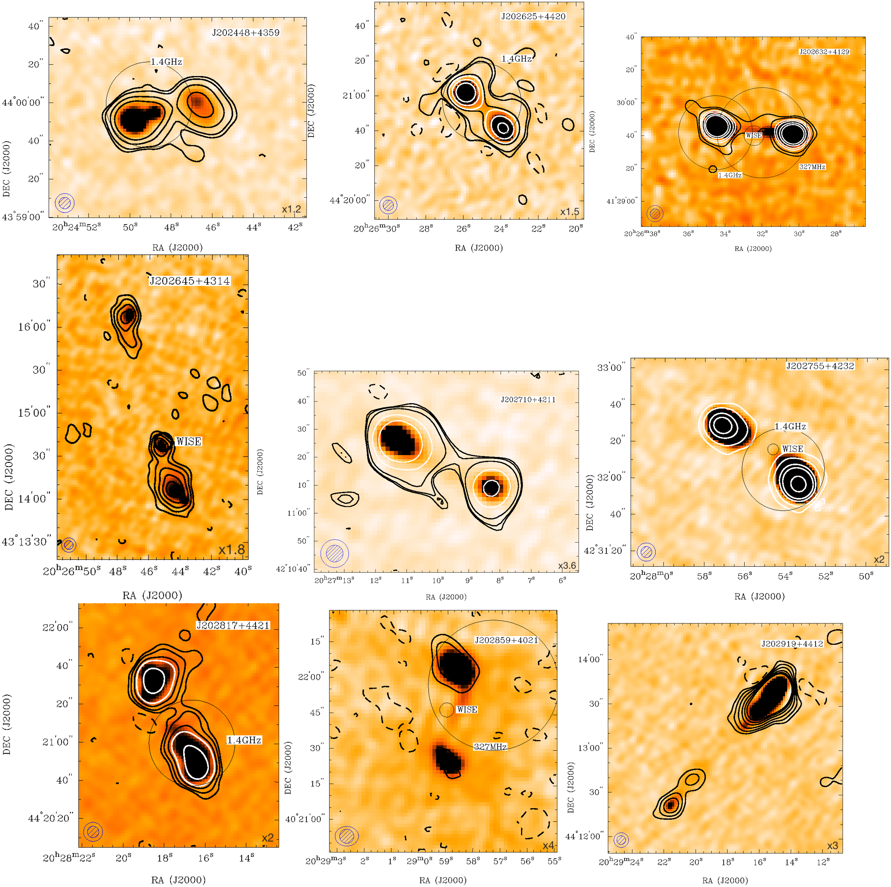
J202422+425722 (#18), J202448+435956 (#19), and J202625+442048 (#20). Each of these sources have coincident NVSS components, all unresolved (see Figures A2, A3 and Table 2).
J202632+412942 (#21) and J202755+423215 (#24). For both sources there are possible associations at the infrared band, WISEA J202634.96
 $+$
412943.8 and WISEA J202755.97
$+$
412943.8 and WISEA J202755.97
 $+$
423224.3, respectively. Besides, the two sources are also unresolved NVSS components. Moreover, the source #21 has positional coincidence with a WSRTGP catalogue record; see Figures A3 and C1.
$+$
423224.3, respectively. Besides, the two sources are also unresolved NVSS components. Moreover, the source #21 has positional coincidence with a WSRTGP catalogue record; see Figures A3 and C1.
J202645+431435 (#22). There is one possible association at infrared frequencies for this source (WISEA J202645.01+431439.8), which could be pinpointing the host galaxy, see Figures A3 and C1. The morphology of this source seems to indicate that the nucleus is closer to the southern lobe.
J202710+421113 (#23) and J202817+442114 (#25). There are just one detection at other frequencies for #25, for which there is an NVSS component overlapping its southern lobe (NVSS ID: J202816+442100), Figure A3.
J202919
 $+$
441341 (#27). There are no associations at other wavelengths. The intensity distribution at both radio bands is complex. We may be looking at a double-lobed source, where projection effects play an important role, see Figure A3. The possibility that we were looking at just one lobe (to the north) and that the southern component is the core seems unlikely, since this latter source do not present the flat spectral index expected from cores.
$+$
441341 (#27). There are no associations at other wavelengths. The intensity distribution at both radio bands is complex. We may be looking at a double-lobed source, where projection effects play an important role, see Figure A3. The possibility that we were looking at just one lobe (to the north) and that the southern component is the core seems unlikely, since this latter source do not present the flat spectral index expected from cores.
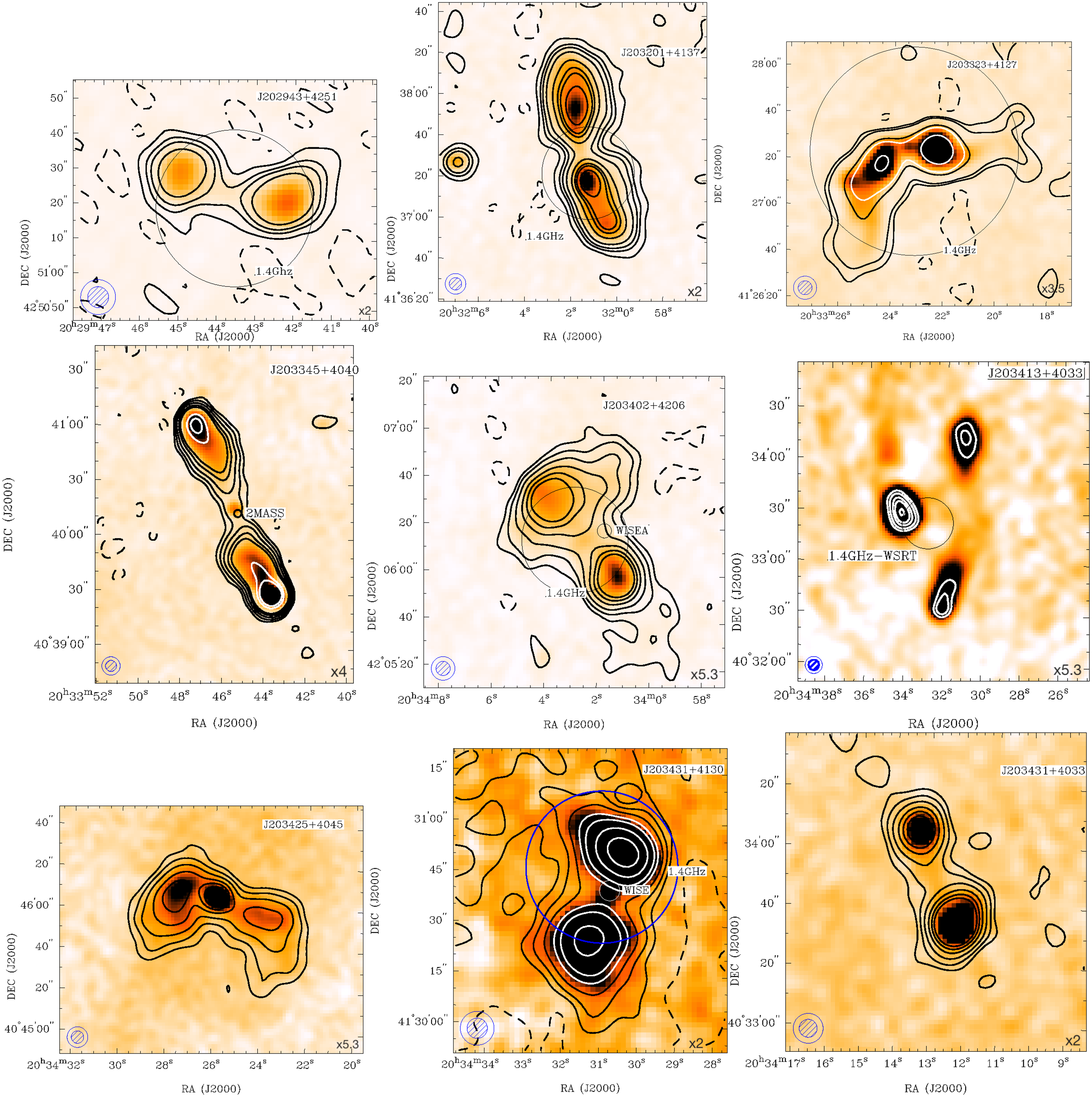
J202943
 $+$
425122 (#28). There is one counterpart at radio frequencies. It is reported in the NVSS catalogue (NVSS ID: J202943+425119), see Figure A4 and Table 2; the source is unresolved.
$+$
425122 (#28). There is one counterpart at radio frequencies. It is reported in the NVSS catalogue (NVSS ID: J202943+425119), see Figure A4 and Table 2; the source is unresolved.
J203201
 $+$
413730 (#29). For this source, there are several counterparts at radio frequencies. Is also known as NVSS J203201+413722 and is unresolved. Martí et al. (Reference Martí, Paredes, Ishwara Chandra and Bosch-Ramon2007) studied it in detail; they proposed it as a radio galaxy which might suffered different episodes of jet activity (see Figure A4). The authors observed the field using the VLA C+D array configuration at 5 GHz as well as the GMRT at 610 MHz. These observations, along with a marginal Chandra X-ray detection in the vicinity of #29 reported by Butt et al. (Reference Butt, Combi, Drake, Finley, Konopelko, Lister, Rodriguez, Shepherd, Ritz, Michelson and Meegan2007), made it a radio galaxy candidate with an optically-thick compact core (Martí et al., Reference Martí, Paredes, Ishwara Chandra and Bosch-Ramon2007). The two lobes of #29 were also reported by Setia Gunawan et al. (Reference Setia Gunawan, de Bruyn, van der Hucht and Williams2003) at their two observing bands; they named them as SBHW-217 (
$+$
413730 (#29). For this source, there are several counterparts at radio frequencies. Is also known as NVSS J203201+413722 and is unresolved. Martí et al. (Reference Martí, Paredes, Ishwara Chandra and Bosch-Ramon2007) studied it in detail; they proposed it as a radio galaxy which might suffered different episodes of jet activity (see Figure A4). The authors observed the field using the VLA C+D array configuration at 5 GHz as well as the GMRT at 610 MHz. These observations, along with a marginal Chandra X-ray detection in the vicinity of #29 reported by Butt et al. (Reference Butt, Combi, Drake, Finley, Konopelko, Lister, Rodriguez, Shepherd, Ritz, Michelson and Meegan2007), made it a radio galaxy candidate with an optically-thick compact core (Martí et al., Reference Martí, Paredes, Ishwara Chandra and Bosch-Ramon2007). The two lobes of #29 were also reported by Setia Gunawan et al. (Reference Setia Gunawan, de Bruyn, van der Hucht and Williams2003) at their two observing bands; they named them as SBHW-217 (
 $S_{\rm 350MHz}=85\pm 5\,\mathrm{mJy}$
,
$S_{\rm 350MHz}=85\pm 5\,\mathrm{mJy}$
,
 $SC_{\rm 1400MHz}=36\pm 5\,\mathrm{mJy}$
) northern lobe and SBHW-218 (
$SC_{\rm 1400MHz}=36\pm 5\,\mathrm{mJy}$
) northern lobe and SBHW-218 (
 $S_{\rm 350MHz}=122\pm 35\,\mathrm{mJy}$
,
$S_{\rm 350MHz}=122\pm 35\,\mathrm{mJy}$
,
 $SC_{\rm 1400MHz}=39\pm 5\,\mathrm{mJy}$
) southern lobe, where the quoted integrated fluxes SC at 1400 MHz were derived from images convolved to the 325 MHz beam.
$SC_{\rm 1400MHz}=39\pm 5\,\mathrm{mJy}$
) southern lobe, where the quoted integrated fluxes SC at 1400 MHz were derived from images convolved to the 325 MHz beam.
J203323
 $+$
412720 (#30) and J203402
$+$
412720 (#30) and J203402
 $+$
420615 (#32). The source #30 was previously reported by Martí et al. (Reference Martí, Paredes, Ishwara Chandra and Bosch-Ramon2007) and is also an unresolved NVSS component. The source #32 has one infrared counterpart (WISEA J203401.86
$+$
420615 (#32). The source #30 was previously reported by Martí et al. (Reference Martí, Paredes, Ishwara Chandra and Bosch-Ramon2007) and is also an unresolved NVSS component. The source #32 has one infrared counterpart (WISEA J203401.86
 $+$
420618.2), and a radio counterpart which is an unresolved NVSS component, see Figures A4 and C1.
$+$
420618.2), and a radio counterpart which is an unresolved NVSS component, see Figures A4 and C1.
J203345
 $+$
404015 (#31). There is one possible association at infrared frequencies, with the object 2MASS J20334540+4040133. At radio frequencies, the NW lobe was reported in WSTRGP (Taylor et al., Reference Taylor, Goss, Coleman, van Leeuwen and Wallace1996) and both lobes were reported by Setia Gunawan et al. (Reference Setia Gunawan, de Bruyn, van der Hucht and Williams2003), at two bands; the ones here called NW, as SBHW-106 (
$+$
404015 (#31). There is one possible association at infrared frequencies, with the object 2MASS J20334540+4040133. At radio frequencies, the NW lobe was reported in WSTRGP (Taylor et al., Reference Taylor, Goss, Coleman, van Leeuwen and Wallace1996) and both lobes were reported by Setia Gunawan et al. (Reference Setia Gunawan, de Bruyn, van der Hucht and Williams2003), at two bands; the ones here called NW, as SBHW-106 (
 $S_{\rm 350MHz} = 75\pm 12\,\mathrm{mJy}$
,
$S_{\rm 350MHz} = 75\pm 12\,\mathrm{mJy}$
,
 $SC_{\rm 1400MHz}=25\pm 4\,\mathrm{mJy}$
), and SE, as SBHW-104 (
$SC_{\rm 1400MHz}=25\pm 4\,\mathrm{mJy}$
), and SE, as SBHW-104 (
 $S_{\rm 350MHz} = 82\pm 4\,\mathrm{mJy}$
,
$S_{\rm 350MHz} = 82\pm 4\,\mathrm{mJy}$
,
 $SC_{\rm 1400MHz} = 34\pm 7\,\mathrm{mJy}$
); see Figures A4 and C1. As a complement we show the spectral index map as well as the error map in Figure B1.
$SC_{\rm 1400MHz} = 34\pm 7\,\mathrm{mJy}$
); see Figures A4 and C1. As a complement we show the spectral index map as well as the error map in Figure B1.
J203413
 $+$
403349 (#33). Eastern to this double-lobed source there is a third source (
$+$
403349 (#33). Eastern to this double-lobed source there is a third source (
 $\sim40"$
apart, and 30
$\sim40"$
apart, and 30
 $^{\prime\prime}$
in size); Setia Gunawan et al. (Reference Setia Gunawan, de Bruyn, van der Hucht and Williams2003) reported 1.4 GHz WSRT emission at its position, from data with angular resolution of 13
$^{\prime\prime}$
in size); Setia Gunawan et al. (Reference Setia Gunawan, de Bruyn, van der Hucht and Williams2003) reported 1.4 GHz WSRT emission at its position, from data with angular resolution of 13
 $^{\prime\prime}$
. We measured
$^{\prime\prime}$
. We measured
 $S_{\rm 325MHz} = 134\pm 16\,\mathrm{mJy}$
and
$S_{\rm 325MHz} = 134\pm 16\,\mathrm{mJy}$
and
 $SC_{\rm 610MHz} = 68\pm 8\,\mathrm{mJy}$
for this third source; the spectral index is then
$SC_{\rm 610MHz} = 68\pm 8\,\mathrm{mJy}$
for this third source; the spectral index is then
 $\alpha_{325}^{610}=-1.7\pm0.3$
. The angular resolutions at the three bands (325, 610, and 1400 MHz) are sufficient to clearly detach the three sources; besides, the northern and southern lobes present extension towards each other, challenging a physical association between this eastern source and the double-lobed #33. See Figure A4.
$\alpha_{325}^{610}=-1.7\pm0.3$
. The angular resolutions at the three bands (325, 610, and 1400 MHz) are sufficient to clearly detach the three sources; besides, the northern and southern lobes present extension towards each other, challenging a physical association between this eastern source and the double-lobed #33. See Figure A4.
J203425
 $+$
404605 (#34) and J203431
$+$
404605 (#34) and J203431
 $+$
403332 (#36). We found no detections at other frequencies for these sources. See Figure A4.
$+$
403332 (#36). We found no detections at other frequencies for these sources. See Figure A4.
J203556
 $+$
421744 (#38) and J203720
$+$
421744 (#38) and J203720
 $+$
405941 (#39). There are counterparts at radio frequencies. Both are reported in the NVSS catalogue. Nevertheless, from the NVSS cutouts, only #39 is resolved at 1.4 GHz. The source #38 has a radio counterpart, which is a component of the WSRTGP surveys (Condon et al., Reference Condon, Cotton, Greisen, Yin, Perley, Taylor and Broderick1998; Taylor et al., Reference Taylor, Goss, Coleman, van Leeuwen and Wallace1996) and also one X-ray possible counterpart (SSTSL2 J203557.22+421744.0, Evans et al., Reference Evans2010). See Figure A5.
$+$
405941 (#39). There are counterparts at radio frequencies. Both are reported in the NVSS catalogue. Nevertheless, from the NVSS cutouts, only #39 is resolved at 1.4 GHz. The source #38 has a radio counterpart, which is a component of the WSRTGP surveys (Condon et al., Reference Condon, Cotton, Greisen, Yin, Perley, Taylor and Broderick1998; Taylor et al., Reference Taylor, Goss, Coleman, van Leeuwen and Wallace1996) and also one X-ray possible counterpart (SSTSL2 J203557.22+421744.0, Evans et al., Reference Evans2010). See Figure A5.
J201836
 $+$
430018 (#40) and J202220
$+$
430018 (#40) and J202220
 $+$
450835 (#42). There are possible associations at infrared frequencies for both sources; one for #40 (WISEA J201836.53
$+$
450835 (#42). There are possible associations at infrared frequencies for both sources; one for #40 (WISEA J201836.53
 $+$
430018.7) and two for #42 (2MASS J20221985
$+$
430018.7) and two for #42 (2MASS J20221985
 $+$
4508338 and WISEA J202219.75
$+$
4508338 and WISEA J202219.75
 $+$
450834.5). Besides, #42 was also reported as an NVSS component, the source is unresolved. See Figures A6 and C2.
$+$
450834.5). Besides, #42 was also reported as an NVSS component, the source is unresolved. See Figures A6 and C2.
J203755
 $+$
401328 (#43). There is one counterpart at radio frequencies. The source is listed in the NVSS catalogue, it is unresolved. See Figure A6.
$+$
401328 (#43). There is one counterpart at radio frequencies. The source is listed in the NVSS catalogue, it is unresolved. See Figure A6.
4.4. Galactic sources
In the sample of double-lobed sources studied here, there are a few with flat or positive spectrum, for which non-thermal radiation mechanisms do not apply. Their emission can be explained advocating thermal processes, by close by (Galactic) plasma media, which emit either under optically thick or thin regimes (Osterbrock, Reference Osterbrock1989).
J202859
 $+$
402141 (#26). This source shows one possible counterpart, nearby the geometric centre and at infrared frequencies (WISEA J202858.96
$+$
402141 (#26). This source shows one possible counterpart, nearby the geometric centre and at infrared frequencies (WISEA J202858.96
 $+$
402146.8), and another at radio frequencies (WSRTGP component); see Figures A3 and C1. The spectral index of the northern lobe is close to zero, while that of the southern lobe is
$+$
402146.8), and another at radio frequencies (WSRTGP component); see Figures A3 and C1. The spectral index of the northern lobe is close to zero, while that of the southern lobe is
 $>1$
, see Table 1. We note that the spectral index error values are high, because the signal-to-noise at the 325 MHz image was low at the position of this source. However, both indices are consistent with those corresponding to Galactic emission. Due to that, we propose that #26 belongs to the Galaxy.
$>1$
, see Table 1. We note that the spectral index error values are high, because the signal-to-noise at the 325 MHz image was low at the position of this source. However, both indices are consistent with those corresponding to Galactic emission. Due to that, we propose that #26 belongs to the Galaxy.
J203431
 $+$
413037 (#35). For this source there is one infrared detection onto the bridge, coincident with the proposed nucleus, WISEA J203433.70+412953.7 and one counterpart at radio frequencies (NVSS component, ID: J203431+413046, unresolved); see Figures A4 and C2. Besides, there is an HII region at
$+$
413037 (#35). For this source there is one infrared detection onto the bridge, coincident with the proposed nucleus, WISEA J203433.70+412953.7 and one counterpart at radio frequencies (NVSS component, ID: J203431+413046, unresolved); see Figures A4 and C2. Besides, there is an HII region at
 $RA, Dec({\rm J2000})\,{=}\,$
20:34:31.9,
$RA, Dec({\rm J2000})\,{=}\,$
20:34:31.9,
 $+$
41:30:52 (G080.522+00.714, Anderson et al., Reference Anderson, Armentrout, Johnstone, Bania, Balser, Wenger and Cunningham2015). The spectral index suggests that it is a Galactic object.
$+$
41:30:52 (G080.522+00.714, Anderson et al., Reference Anderson, Armentrout, Johnstone, Bania, Balser, Wenger and Cunningham2015). The spectral index suggests that it is a Galactic object.
4.5. Dubious cases
Besides the (37+2) double-lobed sources already identified either as extragalactic or Galactic, there remain four cases in which the true nature is not straightforward to unveil, and are analysed below.
J201512+410457 (#3) There are no association at other frequencies for this source; see Figure A1. The radio image at 610 MHz shows that the components present a kind of extension towards each other. Taking this into account, and the fact that the spectral index of both components (similar values) is below
 $-0.7$
, we favour an extragalactic origin for this object.
$-0.7$
, we favour an extragalactic origin for this object.
J202058
 $+$
444050 (#9). This source has counterparts at radio frequencies. Each lobe candidate is coincident with a NVSS component; see Figure A1. The northern one presents a negative spectral index (
$+$
444050 (#9). This source has counterparts at radio frequencies. Each lobe candidate is coincident with a NVSS component; see Figure A1. The northern one presents a negative spectral index (
 $-0.7\pm0.1$
), while the spectral index of the southern one is close to
$-0.7\pm0.1$
), while the spectral index of the southern one is close to
 $-0.1$
. This led us to propose that instead of a double-lobed source, it could well be two different objects, an extragalactic (northern) one and the other of Galactic nature. An alternate possibility is that the southern component is a radio core, of which only the northern lobe is being detected. The sizes of each object are 45 and 20 arcsec, north and south respectively, separated by a distance of 2 arcmin. The evidence gathered is not enough to confirm this candidate as a double-lobed source.
$-0.1$
. This led us to propose that instead of a double-lobed source, it could well be two different objects, an extragalactic (northern) one and the other of Galactic nature. An alternate possibility is that the southern component is a radio core, of which only the northern lobe is being detected. The sizes of each object are 45 and 20 arcsec, north and south respectively, separated by a distance of 2 arcmin. The evidence gathered is not enough to confirm this candidate as a double-lobed source.
J203529
 $+$
403201 (#37). There are no detections at other frequencies at its position; see Figure A5.The spectral indices of both lobes, separated 45 arcsec, are quite different; in particular the one associated with SW lobe, which is close to zero, see Table 1. A possible scenario as an extragalactic source, is that the SW component is a bright hotspot, with its flat spectrum emission being the reason why the spectral index is so different from the NE component.
$+$
403201 (#37). There are no detections at other frequencies at its position; see Figure A5.The spectral indices of both lobes, separated 45 arcsec, are quite different; in particular the one associated with SW lobe, which is close to zero, see Table 1. A possible scenario as an extragalactic source, is that the SW component is a bright hotspot, with its flat spectrum emission being the reason why the spectral index is so different from the NE component.
J201841
 $+$
431844 (#41) shows emission that resembles two highly collimated jets extending along 7 arcmin on the sky. It presents a knot in between the two lobes, indicative of a possible nucleus. The source is not covered by our 325 MHz mosaic image and lacks of infrared or radio putative counterparts; see Figure A6. Notwithstanding, the morphology of the object is typical of AGN-like sources.
$+$
431844 (#41) shows emission that resembles two highly collimated jets extending along 7 arcmin on the sky. It presents a knot in between the two lobes, indicative of a possible nucleus. The source is not covered by our 325 MHz mosaic image and lacks of infrared or radio putative counterparts; see Figure A6. Notwithstanding, the morphology of the object is typical of AGN-like sources.
5. Discussion
5.1. Generalities on spectral indices
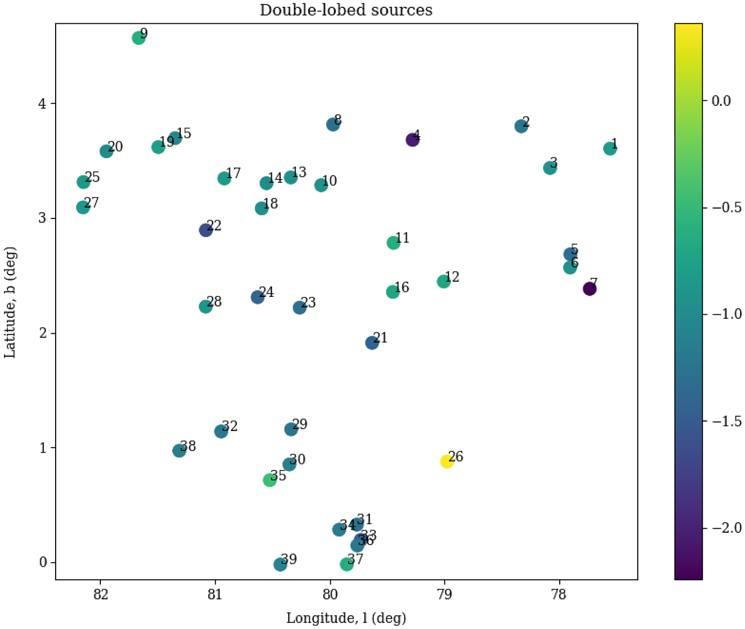
Thirty nine out of the 43 candidates presented in Table 1 were observed at the 2 GMRT bands (325 and 610 MHz), allowing them to retrieve information on their spectral indices. We plotted the layout of those 39 sources in the RA-Dec sky, including a spectral index scale (Figure 2). No trends are recognised, along a
 $\sim 5 \times 5 \mathrm{deg}^2$
area (
$\sim 5 \times 5 \mathrm{deg}^2$
area (
 $0^{\circ} \leq b < 5^{\circ}$
), both with regards to the indices and the location of the sources relative to the Galactic plane.
$0^{\circ} \leq b < 5^{\circ}$
), both with regards to the indices and the location of the sources relative to the Galactic plane.
Layout of the observed double-lobed sources in Galactic coordinates, with their spectral indices represented with colours, according to the scale at the right.
Number of candidates with spectral index information, as a function of their total spectral index (
 $\alpha_{\rm T}$
) between 325 MHz and 610 MHz, for the 39 double-lobed detected at both frequency bands with the GMRT (in blue), and for the sources #42, #43 between 610 MHz and 1400 MHz (in orange).
$\alpha_{\rm T}$
) between 325 MHz and 610 MHz, for the 39 double-lobed detected at both frequency bands with the GMRT (in blue), and for the sources #42, #43 between 610 MHz and 1400 MHz (in orange).
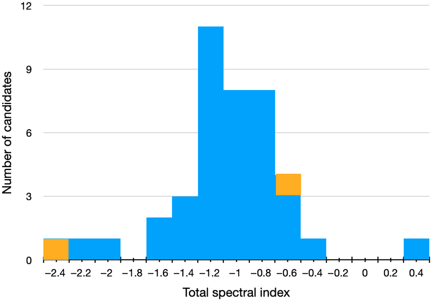
The total spectral index values, derived using the integrated flux density along the whole candidate including material in-between lobes, remain in the interval [
 $-2.5$
,
$-2.5$
,
 $+0.5$
] (see Figure 3). The median spectral index value is
$+0.5$
] (see Figure 3). The median spectral index value is
 $-1.0\pm0.1$
. This is in line with the fact that at the observed bands, the processes involved in non-thermal emission make sources brighter than those related to thermal sources, especially in the case of non-extended ones. In addition, the strategy followed when imaging the original mosaics was to use a weighting scheme aimed to outline discrete sources against diffuse or extended emission.
$-1.0\pm0.1$
. This is in line with the fact that at the observed bands, the processes involved in non-thermal emission make sources brighter than those related to thermal sources, especially in the case of non-extended ones. In addition, the strategy followed when imaging the original mosaics was to use a weighting scheme aimed to outline discrete sources against diffuse or extended emission.
For those (amongst the more extended) sources with a high signal-to-noise ratio (
 $>$
21), we built the spectral index distribution maps; they are shown in Figure B1. The higher
$>$
21), we built the spectral index distribution maps; they are shown in Figure B1. The higher
 $\alpha$
values in the central region are indicative of the nucleus of an extragalactic source.
$\alpha$
values in the central region are indicative of the nucleus of an extragalactic source.
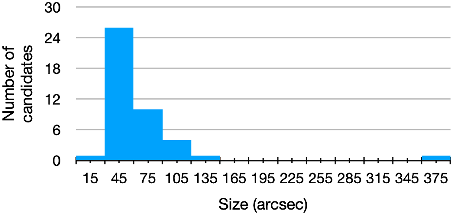
For completeness, we present in Figure 4 the distribution of the total sizes of the 43 candidates (Table 1), as seen in the 610 MHz band.
Distribution of sizes of the 43 double-lobed candidates. The extension of the sources ranged from
 $\sim$
25 arcsec up to
$\sim$
25 arcsec up to
 $\sim$
375 arcsec (
$\sim$
375 arcsec (
 $\sim$
7 arcmins).
$\sim$
7 arcmins).
5.2. Recap on cross-identifications
The cross-identification of the 43 candidates with previous surveys such as the NVSS contributed to examining each candidate’s nature, and helped as verification of the detections presented here (see Section 4).
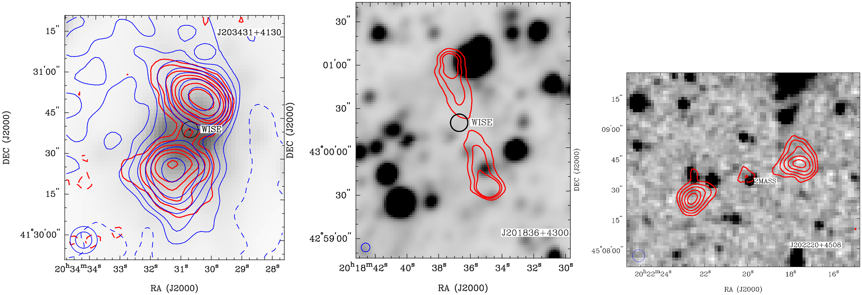
We found 14 IR detections overlapping the nucleus or proposed geometric centre of 12 radio candidates reported along Section 4. Out of these 12 positional coincidences, 9 were only WISE sources, 1 was a 2MASS, and for the remaining 2, we found sources in both the WISE and 2MASS catalogues. The search criteria for the positional overlapping is given Section 4.2. The location of those IR sources are shown in the radio images (Figures A1–A6), labelled as ‘WISE’ and ‘2MASS’. We present in Figures C1 and C2 the infrared images towards the mentioned eleven candidate. We superposed the 325 and 610 MHz emission contours, which allowed us to explore the association between the IR sources and the double-lobed candidates.
The X-ray counterpart found favours the extragalactic origin of source #38, and might indicate that this source is at a closer distance than the rest, see, e.g., Elvis et al. (Reference Elvis, Maccacaro, Wilson, Ward, Penston, Fosbury and Perola1978); Masetti et al. (Reference Masetti2013); Lanzuisi et al. (Reference Lanzuisi2013) and references therein.
5.3. The extragalactic double-lobed sources
After the careful inspection of the 43 double-lobed source candidates presented in this work, and taking into account all the information collected, we found that 37 of them are compatible with an extragalactic nature. For those sources that we proposed a WISE source as a possible candidate, which could be associated with the host galaxy, we estimated the WISE colours W1–W2 and W2–W3, following Gürkan et al. (Reference Gürkan, Hardcastle and Jarvis2014). The values that we obtained (W1–W2 < 0.2 and W2–W3 < 5.8) are compatible with those shown by radio-loud AGNs (see Figure 3 in Gürkan et al., Reference Gürkan, Hardcastle and Jarvis2014). Amongst the 37 sources we found some of them with peculiar morphology such as:
-
#19, #30, and #34 that resemble head–tail galaxies like the ones compiled by Pal & Kumari (Reference Pal and Kumari2021), see, for example, their Figure 2.
-
#29, which seems to be of FRI type.
5.4. On ultra-steep spectrum sources
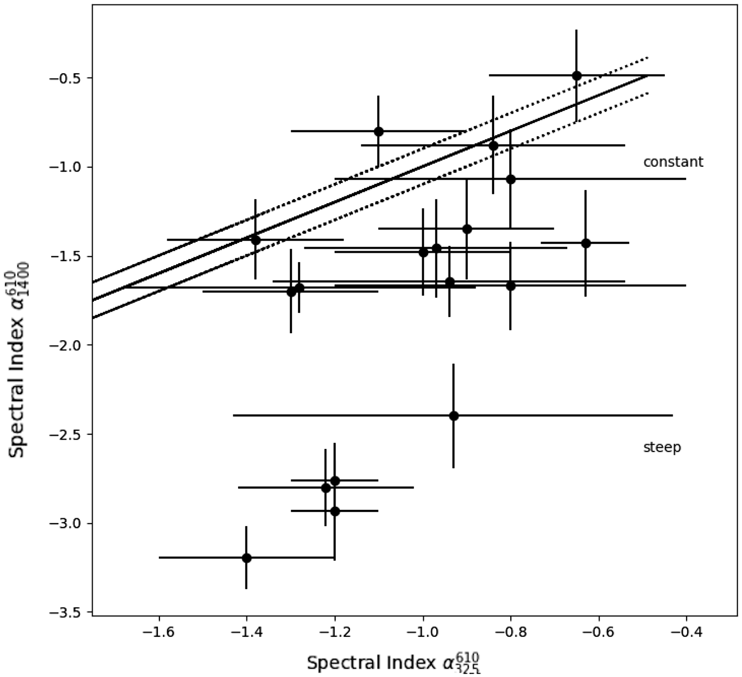
The existence of a radio counterpart at 1.4 GHz allowed us to test for ultra-steep spectrum sources (USS), i.e., objects with
 $\alpha \leq -1.3$
. Saxena et al. (Reference Saxena2018) searched USS as proxies of high-redshift radio galaxies (HzRGs), for which they requested additional characteristics. The authors identified HzRG through a radio colour-colour plot (sources with
$\alpha \leq -1.3$
. Saxena et al. (Reference Saxena2018) searched USS as proxies of high-redshift radio galaxies (HzRGs), for which they requested additional characteristics. The authors identified HzRG through a radio colour-colour plot (sources with
 $\alpha_{1400}^{610}<-1.5$
, see Figure 5), the absence of optically identified counterparts and angular sizes smaller than 30
$\alpha_{1400}^{610}<-1.5$
, see Figure 5), the absence of optically identified counterparts and angular sizes smaller than 30
 $^{\prime\prime}$
(see also references therein). Then, following Saxena et al. (Reference Saxena2018), and for the sources detected at both GMRT bands that possess a radio counterpart at 1.4 GHz, we built the radio colour-colour diagram
$^{\prime\prime}$
(see also references therein). Then, following Saxena et al. (Reference Saxena2018), and for the sources detected at both GMRT bands that possess a radio counterpart at 1.4 GHz, we built the radio colour-colour diagram
 $\alpha_{325}^{610}$
vs
$\alpha_{325}^{610}$
vs
 $\alpha_{1\,400}^{610}$
; see Figure 5. The plot reveals that the majority of the double-lobed sources have a constant or a steep spectrum. In particular, there are five sources at the loci of USS ones, with
$\alpha_{1\,400}^{610}$
; see Figure 5. The plot reveals that the majority of the double-lobed sources have a constant or a steep spectrum. In particular, there are five sources at the loci of USS ones, with
 $\alpha << -1.5$
: #6, #21, #29, #30 and #32. It can be appreciated in Table 2 that these five sources, together with #43, are the ones with the steepest spectral indices,
$\alpha << -1.5$
: #6, #21, #29, #30 and #32. It can be appreciated in Table 2 that these five sources, together with #43, are the ones with the steepest spectral indices,
 $\alpha \leq -2.3$
; #43 was not covered by our 325 MHz image and, it will not be analysed. Only one of the sources has an extension of
$\alpha \leq -2.3$
; #43 was not covered by our 325 MHz image and, it will not be analysed. Only one of the sources has an extension of
 $\sim30''$
(source #6). New observations at 1.4 GHz, with better sensitivity and higher angular resolution, are needed to confirm whether candidate #6 is a USS source.
$\sim30''$
(source #6). New observations at 1.4 GHz, with better sensitivity and higher angular resolution, are needed to confirm whether candidate #6 is a USS source.
Radio colour-colour diagram. The spectral indices of the detected double-lobed sources between 325 and 610 MHz versus the spectral indices between 1400 and 610 MHz. The solid and dashed lines mark the constant spectral index at both radio colours and the adopted errors of 0.1. The sources with
 $\alpha_{1400}^{610}<<-1.5$
are considered to be ultra-steep spectrum sources.
$\alpha_{1400}^{610}<<-1.5$
are considered to be ultra-steep spectrum sources.
6. Statistics and conclusions
-
In a region of
 $19.7\,\mathrm{deg}^2$
of the sky, 43 probable double-lobed sources were found at 610 MHz, 39 of them also at 325 MHz.
$19.7\,\mathrm{deg}^2$
of the sky, 43 probable double-lobed sources were found at 610 MHz, 39 of them also at 325 MHz. -
The angular resolutions of the data sets were 6
$^{\prime\prime}$
to 10
$^{\prime\prime}$
, and the average sensitivities, 0.2 and
$0.5\,\mathrm{mJy\,beam}^{-1}$
(at 610 and 325 MHz, respectively). -
The extension of the sources ranged from
$\sim$
25 arcsec up to
$\sim 7$
arcmins. -
Twenty one out of the 43 sources have a bridge.
-
Eleven out of the 43 sources have a detected nucleus.
-
Thirty seven out of the 43 sources have spectral indices characteristic of extragalactic objects, probably AGNs.
-
Nine out of the 37 proposed as extragalactic sources present infrared sources at the position of a putative nucleus.
-
Two out of the 43 sources have flat or positive spectral indices, favouring a Galactic origin.
-
For one of the 43 sources, the two emitting objects are probably not physically related.
-
Three out of the 43 remains as dubious cases, though with feature(s) compatible with an extragalactic nature.
-
The median spectral index value of the extragalactic sources is
$-1.0\pm0.1$
. Five extragalactic sources present an ultra-steep spectra. Only one of them (#6) has a small size (
$\leq 30''$
) consistent with a high-redshift radio galaxy. -
Although the large angular scale probed at the highest observing band was 17
$^{\prime}$
, no sources with extension above 7 arcmin were detected.


Acknowledgements
The radio data presented here were obtained with the Giant Metrewave Radio Telescope (GMRT). The GMRT is operated by the National Centre for Radio Astrophysics of the Tata Institute of Fundamental Research. We thank the staff of the GMRT that made these observations possible. This research has made use of the NASA/IPAC extragalactic database (NED) that is operated by the Jet Propulsion Laboratory, California Institute of Technology, under contract with the National Aeronautics and Space Administration and also we made use of the SIMBAD database, operated at CDS, Strasbourg, France, and of NASA’s Astrophysics Data System bibliographic series. J.S. and P.B. acknowledge support from ANPCyT PICT 0773–2017. The authors want to thank the anonymous referee for the careful reading of the manuscript and their many insightful comments and suggestions. C.H.I.C. acknowledges the support of the Department of Atomic Energy, Government of India, under the project 12-R&D-TFR-5.02-0700.
A. Appendix
In this appendix we present the GMRT images of 39 double-lobed source candidates at 610 and 325 MHz, and the remaining 4—out of a total of 43—only observed at 610 MHz (Figures A1 to A6). The candidates showed radio emission at rather different scales. The one with the lowest
 $\sigma$
value is #12 (
$\sigma$
value is #12 (
 $\sigma_{12} = 0.1\,\mathrm{mJy\,beam}^{-1}$
). To allow comparison amongst sub-figures, we added in the bottom right corner of each one a scale number (preceded with an ‘x’), which represents the factor to multiply
$\sigma_{12} = 0.1\,\mathrm{mJy\,beam}^{-1}$
). To allow comparison amongst sub-figures, we added in the bottom right corner of each one a scale number (preceded with an ‘x’), which represents the factor to multiply
 $\sigma_{12}$
to get the
$\sigma_{12}$
to get the
 $\sigma$
of the candidate sub-figure.
$\sigma$
of the candidate sub-figure.
For some of the candidates (#4, #5, #15, #31), we show the spectral index distribution and error maps (Figure B1). And for those probable galaxies with putative infrared counterparts, we present the radio contours on top of the IR images (Figures C1 and C2).
GMRT images of the double-lobed sources at 610 MHz (colour scale) and 325 MHz (contours). The contour levels and colour scale interval for each source are as follows: #1-J201255+404423:
 $-2.5$
, 2.5, 3, 15, 27, 60, and 90, in units of
$-2.5$
, 2.5, 3, 15, 27, 60, and 90, in units of
 $\sigma (=0.18\,\mathrm{mJy\,beam}^{-1});\ [1.6, 20]\,\mathrm{mJy\,beam}^{-1}$
. #2-J201418+412931:
$\sigma (=0.18\,\mathrm{mJy\,beam}^{-1});\ [1.6, 20]\,\mathrm{mJy\,beam}^{-1}$
. #2-J201418+412931:
 $-2.5$
, 2.5, 3, 15, 27, 60, and 90, in units of
$-2.5$
, 2.5, 3, 15, 27, 60, and 90, in units of
 $\sigma (=0.45\,\mathrm{mJy\,beam}^{-1});\ [3, 13]\,\mathrm{mJy\,beam}^{-1}$
.#3-J201512+410457:
$\sigma (=0.45\,\mathrm{mJy\,beam}^{-1});\ [3, 13]\,\mathrm{mJy\,beam}^{-1}$
.#3-J201512+410457:
 $-2.5$
, 2.5, 5, 9, 15, 21, and 41, in units of
$-2.5$
, 2.5, 5, 9, 15, 21, and 41, in units of
 $\sigma (=0.45\,\mathrm{mJy\,beam}^{-1});\ [4, 11]\,\mathrm{mJy\,beam}^{-1}$
.#4-J201739+421243:
$\sigma (=0.45\,\mathrm{mJy\,beam}^{-1});\ [4, 11]\,\mathrm{mJy\,beam}^{-1}$
.#4-J201739+421243:
 $-2.5$
, 2.5, 5, 9, 21, and 27, in units of
$-2.5$
, 2.5, 5, 9, 21, and 27, in units of
 $\sigma (=0.2\,\mathrm{mJy\,beam}^{-1};\ [0.4, 4]\,\mathrm{mJy\,beam}^{-1}$
.#5-J201758+403100:
$\sigma (=0.2\,\mathrm{mJy\,beam}^{-1};\ [0.4, 4]\,\mathrm{mJy\,beam}^{-1}$
.#5-J201758+403100:
 $-2.5$
, 2.5, 15, 27, 30, 45, 55, and 100, in units of
$-2.5$
, 2.5, 15, 27, 30, 45, 55, and 100, in units of
 $\sigma (=0.6\,\mathrm{mJy\,beam}^{-1});\ [0.6, 17]\,\mathrm{mJy\,beam}^{-1}$
.#6-J201828+402714:
$\sigma (=0.6\,\mathrm{mJy\,beam}^{-1});\ [0.6, 17]\,\mathrm{mJy\,beam}^{-1}$
.#6-J201828+402714:
 $-2.5$
, 2.5, 3, 15, 27, 60, and 90, in units of
$-2.5$
, 2.5, 3, 15, 27, 60, and 90, in units of
 $\sigma (=0.18\,\mathrm{mJy\,beam}^{-1});\ [6, 21]\,\mathrm{mJy\,beam}^{-1}$
. #7-J201847+401230:
$\sigma (=0.18\,\mathrm{mJy\,beam}^{-1});\ [6, 21]\,\mathrm{mJy\,beam}^{-1}$
. #7-J201847+401230:
 $-2.5$
, 2.5, 5, 9, 11, and 21, in units of
$-2.5$
, 2.5, 5, 9, 11, and 21, in units of
 $\sigma (=1.7\,\mathrm{mJy\,beam}^{-1});\ [6, 21]\,\mathrm{mJy\,beam}^{-1}$
. #8-J201910+425136:
$\sigma (=1.7\,\mathrm{mJy\,beam}^{-1});\ [6, 21]\,\mathrm{mJy\,beam}^{-1}$
. #8-J201910+425136:
 $-2.5$
, 2.5, 3, 6, 9, 15, 21, and 30, in units of
$-2.5$
, 2.5, 3, 6, 9, 15, 21, and 30, in units of
 $\sigma (=0.7\,\mathrm{mJy\,beam}^{-1});\ [0.7, 9]\,\mathrm{mJy\,beam}^{-1}$
. #9-J202058+444050:
$\sigma (=0.7\,\mathrm{mJy\,beam}^{-1});\ [0.7, 9]\,\mathrm{mJy\,beam}^{-1}$
. #9-J202058+444050:
 $-2.5$
, 2.5, 3, 15, 27, 60, and 90, in units of
$-2.5$
, 2.5, 3, 15, 27, 60, and 90, in units of
 $\sigma (=0.15\,\mathrm{mJy\,beam}^{-1});\ [0.7, 9]\,\mathrm{mJy\,beam}^{-1}$
. The synthesised beams are shown at the bottom left corner of each image. NVSS detections are marked with a 45
$\sigma (=0.15\,\mathrm{mJy\,beam}^{-1});\ [0.7, 9]\,\mathrm{mJy\,beam}^{-1}$
. The synthesised beams are shown at the bottom left corner of each image. NVSS detections are marked with a 45
 $^{\prime\prime}$
diameter circle and labelled as ‘1.4 GHz’. For the x factor of the bottom right corner, see text.
$^{\prime\prime}$
diameter circle and labelled as ‘1.4 GHz’. For the x factor of the bottom right corner, see text.

GMRT images of the double-lobed sources at 610 MHz (colour scale) and 325 MHz (contours). The contour levels and colour scale interval for each source are as follows: #10-J202151+423847:
 $-2.5$
, 2.5, 3, and 5, in units of
$-2.5$
, 2.5, 3, and 5, in units of
 $\sigma (=1\,\mathrm{mJy\,beam}^{-1});\ [0.3, 1]\,\mathrm{mJy\,beam}^{-1}$
. #11-J202209+415033:
$\sigma (=1\,\mathrm{mJy\,beam}^{-1});\ [0.3, 1]\,\mathrm{mJy\,beam}^{-1}$
. #11-J202209+415033:
 $-2.5$
, 2.5, 3, 5, and 15, in units of
$-2.5$
, 2.5, 3, 5, and 15, in units of
 $\sigma (=1\,\mathrm{mJy\,beam}^{-1});\ [0.4, 3.9]\,\mathrm{mJy\,beam}^{-1}$
. #12-J202218+411728:
$\sigma (=1\,\mathrm{mJy\,beam}^{-1});\ [0.4, 3.9]\,\mathrm{mJy\,beam}^{-1}$
. #12-J202218+411728:
 $-2.5$
, 2.5, 10, and 30, in units of
$-2.5$
, 2.5, 10, and 30, in units of
 $\sigma (=0.1\,\mathrm{mJy\,beam}^{-1});\ [0.5, 3.8]\,\mathrm{mJy\,beam}^{-1}$
. #13-J202222+425409:
$\sigma (=0.1\,\mathrm{mJy\,beam}^{-1});\ [0.5, 3.8]\,\mathrm{mJy\,beam}^{-1}$
. #13-J202222+425409:
 $-2.5$
, 2.5, 9, 15, 25, and 85, in units of
$-2.5$
, 2.5, 9, 15, 25, and 85, in units of
 $\sigma (=0.87\,\mathrm{mJy\,beam}^{-1});\ [0.3, 6.1]\,\mathrm{mJy\,beam}^{-1}$
. #14-J202315+430252:
$\sigma (=0.87\,\mathrm{mJy\,beam}^{-1});\ [0.3, 6.1]\,\mathrm{mJy\,beam}^{-1}$
. #14-J202315+430252:
 $-2.5$
, 2.5, 9, 15, and 25, in units of
$-2.5$
, 2.5, 9, 15, and 25, in units of
 $\sigma (=0.27\,\mathrm{mJy\,beam}^{-1});\ [0.3, 7.9]\,\mathrm{mJy\,beam}^{-1}$
. #15-J202359+435525:
$\sigma (=0.27\,\mathrm{mJy\,beam}^{-1});\ [0.3, 7.9]\,\mathrm{mJy\,beam}^{-1}$
. #15-J202359+435525:
 $-2.5$
, 2.5, 5, 9, 15, 21, and 27, in units of
$-2.5$
, 2.5, 5, 9, 15, 21, and 27, in units of
 $\sigma (=0.12\,\mathrm{mJy\,beam}^{-1});\ [0.4, 4.2]\,\mathrm{mJy\,beam}^{-1}$
. #16-J202403+413611:
$\sigma (=0.12\,\mathrm{mJy\,beam}^{-1});\ [0.4, 4.2]\,\mathrm{mJy\,beam}^{-1}$
. #16-J202403+413611:
 $-2.5$
, 2.5, 15, 25, 35, 45, and 55, in units of
$-2.5$
, 2.5, 15, 25, 35, 45, and 55, in units of
 $\sigma (=0.2\,\mathrm{mJy\,beam}^{-1});\ [0.4, 4.2]\,\mathrm{mJy\,beam}^{-1}$
. #17-J202413+432220:
$\sigma (=0.2\,\mathrm{mJy\,beam}^{-1});\ [0.4, 4.2]\,\mathrm{mJy\,beam}^{-1}$
. #17-J202413+432220:
 $-2.5$
, 2.5, 5, 15, 21, and 30, in units of
$-2.5$
, 2.5, 5, 15, 21, and 30, in units of
 $\sigma (=0.2\,\mathrm{mJy\,beam}^{-1};\ [1, 4.4]\,\mathrm{mJy\,beam}^{-1}$
.
$\sigma (=0.2\,\mathrm{mJy\,beam}^{-1};\ [1, 4.4]\,\mathrm{mJy\,beam}^{-1}$
.
 $\#$
18-J202422+425722:
$\#$
18-J202422+425722:
 $-2.5$
, 2.5, 5, 15, and 21, in units of
$-2.5$
, 2.5, 5, 15, and 21, in units of
 $\sigma (=0.27\,\mathrm{mJy\,beam}^{-1});\ [6, 21]\,\mathrm{mJy\,beam}^{-1}$
. The synthesised beams are shown at the bottom left corner of each image. NVSS detections are marked with a 45
$\sigma (=0.27\,\mathrm{mJy\,beam}^{-1});\ [6, 21]\,\mathrm{mJy\,beam}^{-1}$
. The synthesised beams are shown at the bottom left corner of each image. NVSS detections are marked with a 45
 $^{\prime\prime}$
diameter circle and labelled as ‘1.4 GHz’. WISE and 2MASS sources are marked and labelled as well. For the x factor of the bottom right corner, see text.
$^{\prime\prime}$
diameter circle and labelled as ‘1.4 GHz’. WISE and 2MASS sources are marked and labelled as well. For the x factor of the bottom right corner, see text.
GMRT images of the double-lobed sources at 610 MHz (colour scale) and 325 MHz (contours). The contour levels and colour scale interval for each source are as follows: #19-J202448+435956:
 $-2.5$
, 2.5, 5, 10, and 27, in units of
$-2.5$
, 2.5, 5, 10, and 27, in units of
 $\sigma(=0.12\,\mathrm{mJy\,beam}^{-1});\ [0.3, 2.6]\,\mathrm{mJy\,beam}^{-1}$
. #20-J202625+442048:
$\sigma(=0.12\,\mathrm{mJy\,beam}^{-1});\ [0.3, 2.6]\,\mathrm{mJy\,beam}^{-1}$
. #20-J202625+442048:
 $-2.5$
, 2.5, 5, 25, 35, 75, and 135, in units of
$-2.5$
, 2.5, 5, 25, 35, 75, and 135, in units of
 $\sigma(=0.15\,\mathrm{mJy\,beam}^{-1});[0.3, 2]\,\mathrm{mJy\,beam}^{-1}$
. #21-J202632+412942:
$\sigma(=0.15\,\mathrm{mJy\,beam}^{-1});[0.3, 2]\,\mathrm{mJy\,beam}^{-1}$
. #21-J202632+412942:
 $-2.5$
, 2.5, 5, 10, 15, 25, and 35, in units of
$-2.5$
, 2.5, 5, 10, 15, 25, and 35, in units of
 $\sigma(=1\,\mathrm{mJy\,beam}^{-1});\ [0.3, 0.6]\,\mathrm{mJy\,beam}^{-1}$
. #22-J202645+431435:
$\sigma(=1\,\mathrm{mJy\,beam}^{-1});\ [0.3, 0.6]\,\mathrm{mJy\,beam}^{-1}$
. #22-J202645+431435:
 $-2.5$
, 2.5, 5, 9, 15, 21, and 27, in units of
$-2.5$
, 2.5, 5, 9, 15, 21, and 27, in units of
 $\sigma(=0.18\,\mathrm{mJy\,beam}^{-1});\ [0.2, 0.7]\,\mathrm{mJy\,beam}^{-1}$
. #23-J202710+421113:
$\sigma(=0.18\,\mathrm{mJy\,beam}^{-1});\ [0.2, 0.7]\,\mathrm{mJy\,beam}^{-1}$
. #23-J202710+421113:
 $-2.5$
, 2.5, 3, 5, 15, and 35, in units of
$-2.5$
, 2.5, 3, 5, 15, and 35, in units of
 $\sigma(=0.36\,\mathrm{mJy\,beam}^{-1});\ [0.3, 3.9]\,\mathrm{mJy\,beam}^{-1}$
. #24-J202755+423215:
$\sigma(=0.36\,\mathrm{mJy\,beam}^{-1});\ [0.3, 3.9]\,\mathrm{mJy\,beam}^{-1}$
. #24-J202755+423215:
 $-2.5$
, 2.5, 30, 50, 130, and 310, in units of
$-2.5$
, 2.5, 30, 50, 130, and 310, in units of
 $\sigma(=0.2\,\mathrm{mJy\,beam}^{-1});\ [0.3, 3.9]\,\mathrm{mJy\,beam}^{-1}$
. #25-J202817+442114:
$\sigma(=0.2\,\mathrm{mJy\,beam}^{-1});\ [0.3, 3.9]\,\mathrm{mJy\,beam}^{-1}$
. #25-J202817+442114:
 $-2.5$
, 2.5, 5, 10, 15, 35, and 85, in units of
$-2.5$
, 2.5, 5, 10, 15, 35, and 85, in units of
 $\sigma(=0.16\,\mathrm{mJy\,beam}^{-1});\ [0.8, 1]\,\mathrm{mJy\,beam}^{-1}$
. #26-J202859+402141:
$\sigma(=0.16\,\mathrm{mJy\,beam}^{-1});\ [0.8, 1]\,\mathrm{mJy\,beam}^{-1}$
. #26-J202859+402141:
 $-2.5$
, 2.5, 5, 9, 15, 21, and 27, in units of
$-2.5$
, 2.5, 5, 9, 15, 21, and 27, in units of
 $\sigma(=0.4\,\mathrm{mJy\,beam}^{-1});\ [0.6, 1.8]\,\mathrm{mJy\,beam}^{-1}$
. #27-J202919+441341
$\sigma(=0.4\,\mathrm{mJy\,beam}^{-1});\ [0.6, 1.8]\,\mathrm{mJy\,beam}^{-1}$
. #27-J202919+441341
 $-2.5$
, 2.5, 5, 9, 15, 21, and 27, in units of
$-2.5$
, 2.5, 5, 9, 15, 21, and 27, in units of
 $\sigma(=0.3\,\mathrm{mJy\,beam}^{-1});\ [0.4, 2]\,\mathrm{mJy\,beam}^{-1}$
. The synthesised beams are shown at the bottom left corner of each image. NVSS and WSRT detections are marked and labelled as ‘1.4 GHz’ and ‘327 MHz’. WISE and 2MASS sources are marked and labelled as well. For the x factor of the bottom right corner, see text.
$\sigma(=0.3\,\mathrm{mJy\,beam}^{-1});\ [0.4, 2]\,\mathrm{mJy\,beam}^{-1}$
. The synthesised beams are shown at the bottom left corner of each image. NVSS and WSRT detections are marked and labelled as ‘1.4 GHz’ and ‘327 MHz’. WISE and 2MASS sources are marked and labelled as well. For the x factor of the bottom right corner, see text.
GMRT images of the double-lobed sources at 610 MHz (colour scale) and 325 MHz (contours). The contour levels and colour scale interval for each source are as follows: #28-J202943+425122:
 $-2.5$
, 2.5, 9, 15, 27 in units of
$-2.5$
, 2.5, 9, 15, 27 in units of
 $\sigma(=0.2\,\mathrm{mJy\,beam}^{-1});\ [0.4, 1]\,\mathrm{mJy\,beam}^{-1}$
. #29-J203201+413730:
$\sigma(=0.2\,\mathrm{mJy\,beam}^{-1});\ [0.4, 1]\,\mathrm{mJy\,beam}^{-1}$
. #29-J203201+413730:
 $-2.5$
, 2.5, 9, 15, 27, 57, 87, 107, and 150, in units of
$-2.5$
, 2.5, 9, 15, 27, 57, 87, 107, and 150, in units of
 $\sigma(=0.2\,\mathrm{mJy\,beam}^{-1});\ [0.4, 1]\,\mathrm{mJy\,beam}^{-1}$
. #30-J203323+412720:
$\sigma(=0.2\,\mathrm{mJy\,beam}^{-1});\ [0.4, 1]\,\mathrm{mJy\,beam}^{-1}$
. #30-J203323+412720:
 $-2.5$
, 2.5, 5, 27, 40, and 100, in units of
$-2.5$
, 2.5, 5, 27, 40, and 100, in units of
 $\sigma(=0.35\,\mathrm{mJy\,beam}^{-1});\ [0.6, 5]\,\mathrm{mJy\,beam}^{-1}$
. #31-J203345+404015:
$\sigma(=0.35\,\mathrm{mJy\,beam}^{-1});\ [0.6, 5]\,\mathrm{mJy\,beam}^{-1}$
. #31-J203345+404015:
 $-2.5$
, 2.5, 5, 9, 15, 21, 55, and 75, in units of
$-2.5$
, 2.5, 5, 9, 15, 21, 55, and 75, in units of
 $\sigma(=0.4\,\mathrm{mJy\,beam}^{-1});\ [0.5, 5]\,\mathrm{mJy\,beam}^{-1}$
. #32-J203402+420615:
$\sigma(=0.4\,\mathrm{mJy\,beam}^{-1});\ [0.5, 5]\,\mathrm{mJy\,beam}^{-1}$
. #32-J203402+420615:
 $-2.5$
, 2.5, 5, 9, 15, 21, and 27, in units of
$-2.5$
, 2.5, 5, 9, 15, 21, and 27, in units of
 $\sigma(=0.53\,\mathrm{mJy\,beam}^{-1});\ [0.4, 10]\,\mathrm{mJy\,beam}^{-1}$
. #33-J203413+403349:
$\sigma(=0.53\,\mathrm{mJy\,beam}^{-1});\ [0.4, 10]\,\mathrm{mJy\,beam}^{-1}$
. #33-J203413+403349:
 $-2.5$
, 2.5, 5, 9, 15, 21, and 27, in units of
$-2.5$
, 2.5, 5, 9, 15, 21, and 27, in units of
 $\sigma(=0.53\,\mathrm{mJy\,beam}^{-1});\ [0.4, 10]\,\mathrm{mJy\,beam}^{-1}$
. #34-J203425+404605:
$\sigma(=0.53\,\mathrm{mJy\,beam}^{-1});\ [0.4, 10]\,\mathrm{mJy\,beam}^{-1}$
. #34-J203425+404605:
 $-2.5$
, 2.5, 5, 9, 15, 21, and 27, in units of
$-2.5$
, 2.5, 5, 9, 15, 21, and 27, in units of
 $\sigma(=0.53\,\mathrm{mJy\,beam}^{-1});\ [0.3, 2.8]\,\mathrm{mJy\,beam}^{-1}$
. #35-J203431+413037:
$\sigma(=0.53\,\mathrm{mJy\,beam}^{-1});\ [0.3, 2.8]\,\mathrm{mJy\,beam}^{-1}$
. #35-J203431+413037:
 $-2.5$
, 2.5, 5, 9, 15, 21, 35, and 55, in units of
$-2.5$
, 2.5, 5, 9, 15, 21, 35, and 55, in units of
 $\sigma(=0.2\,\mathrm{mJy\,beam}^{-1});\ [0.4, 14]\,\mathrm{mJy\,beam}^{-1}$
. #36-J203431+403332:
$\sigma(=0.2\,\mathrm{mJy\,beam}^{-1});\ [0.4, 14]\,\mathrm{mJy\,beam}^{-1}$
. #36-J203431+403332:
 $-2.5$
, 2.5, 5, 9, 15, 21, and 27, in units of
$-2.5$
, 2.5, 5, 9, 15, 21, and 27, in units of
 $\sigma(=0.53\,\mathrm{mJy\,beam}^{-1});\ [0.2, 0.7]\,\mathrm{mJy\,beam}^{-1}$
. The synthesised beams are shown at the bottom left corner of each image. NVSS and WSRT beams detection are marked with a circles and labelled as ‘1.4 GHz’ and ‘1.4GHz-WSRT’. WISE and 2MASS position errors are marked with circles and labelled as well. For the x factor of the bottom right corner, see text.
$\sigma(=0.53\,\mathrm{mJy\,beam}^{-1});\ [0.2, 0.7]\,\mathrm{mJy\,beam}^{-1}$
. The synthesised beams are shown at the bottom left corner of each image. NVSS and WSRT beams detection are marked with a circles and labelled as ‘1.4 GHz’ and ‘1.4GHz-WSRT’. WISE and 2MASS position errors are marked with circles and labelled as well. For the x factor of the bottom right corner, see text.
GMRT images of the double-lobed sources at 610 MHz (colour scale) and 325 MHz (contours). The contour levels and colour scale interval for each source are as follows: #37-J203529+403201:
 $-2.5$
, 2.5, 5, 9, 15, 21, and 27, in units of
$-2.5$
, 2.5, 5, 9, 15, 21, and 27, in units of
 $\sigma(=0.7\,\mathrm{mJy\,beam}^{-1});\ [1, 8]\,\mathrm{mJy\,beam}^{-1}$
. #38-J203556+421744:
$\sigma(=0.7\,\mathrm{mJy\,beam}^{-1});\ [1, 8]\,\mathrm{mJy\,beam}^{-1}$
. #38-J203556+421744:
 $-2.5$
, 2.5, 10, 20, 30, 120, 200, 300, and 500, in units of
$-2.5$
, 2.5, 10, 20, 30, 120, 200, 300, and 500, in units of
 $\sigma(=9\,\mathrm{mJy\,beam}^{-1});\ [3, 237]\,\mathrm{mJy\,beam}^{-1}$
. #39-J203720+405941:
$\sigma(=9\,\mathrm{mJy\,beam}^{-1});\ [3, 237]\,\mathrm{mJy\,beam}^{-1}$
. #39-J203720+405941:
 $-2.5$
, 2.5, and 5, in units of
$-2.5$
, 2.5, and 5, in units of
 $\sigma(=0.2\,\mathrm{mJy\,beam}^{-1});\ [2, 7]\,\mathrm{mJy\,beam}^{-1}$
. The synthesised beams are shown at the bottom left corner of each image. NVSS beam detection is marked with a circle and labelled as ‘1.4 GHz’ while the X-ray detection is shown with a red circle. For the x factor of the bottom right corner, see text.
$\sigma(=0.2\,\mathrm{mJy\,beam}^{-1});\ [2, 7]\,\mathrm{mJy\,beam}^{-1}$
. The synthesised beams are shown at the bottom left corner of each image. NVSS beam detection is marked with a circle and labelled as ‘1.4 GHz’ while the X-ray detection is shown with a red circle. For the x factor of the bottom right corner, see text.
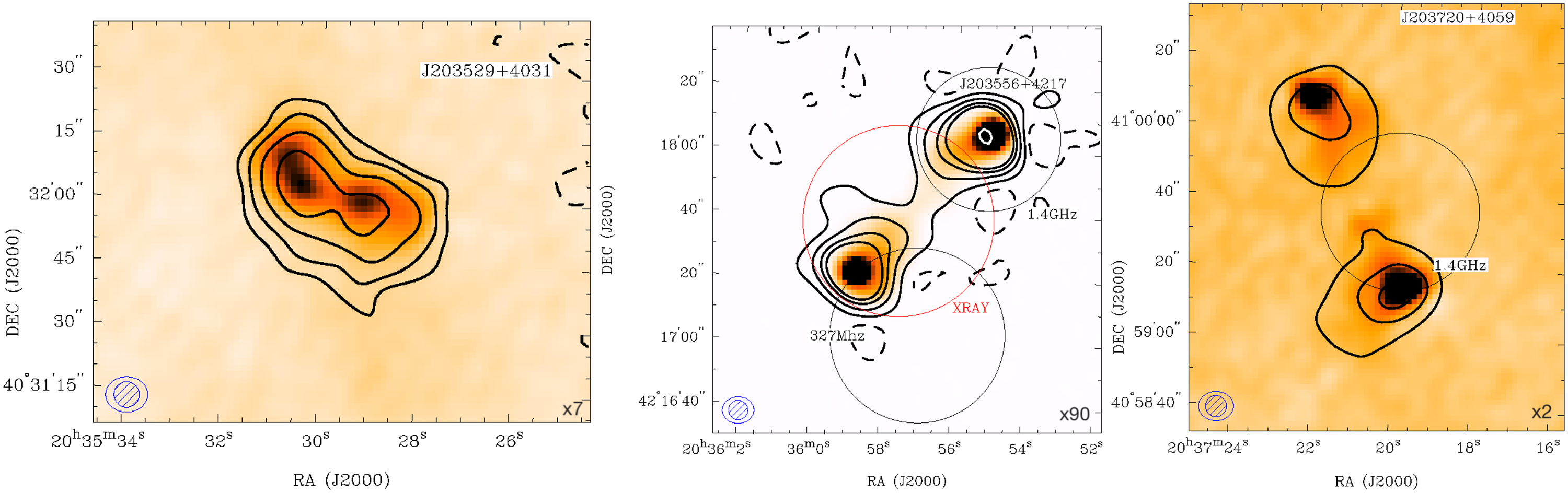
GMRT images of the double-lobed sources at 610 MHz (colour scale). NVSS beam detection is marked with a circle and labelled as ‘1.4 GHz’. WISE and 2MASS position errors are marked with circles and labelled as well. The sources and colour scale interval represented are:
 $\# $
40-J201836+430018: [0.4, 5]
$\# $
40-J201836+430018: [0.4, 5]
 $\mathrm{mJy\,beam}^{-1}$
; #41-J201841+431844: [0.2, 1.6]
$\mathrm{mJy\,beam}^{-1}$
; #41-J201841+431844: [0.2, 1.6]
 $\mathrm{mJy\,beam}^{-1}$
; #42-J202220+450835:
$\mathrm{mJy\,beam}^{-1}$
; #42-J202220+450835:
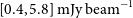 $[0.4, 5.8]\,\mathrm{mJy\,beam}^{-1}$
; #43-J203755+401328:
$[0.4, 5.8]\,\mathrm{mJy\,beam}^{-1}$
; #43-J203755+401328:
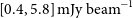 $[0.4, 5.8]\,\mathrm{mJy\,beam}^{-1}$
.
$[0.4, 5.8]\,\mathrm{mJy\,beam}^{-1}$
.
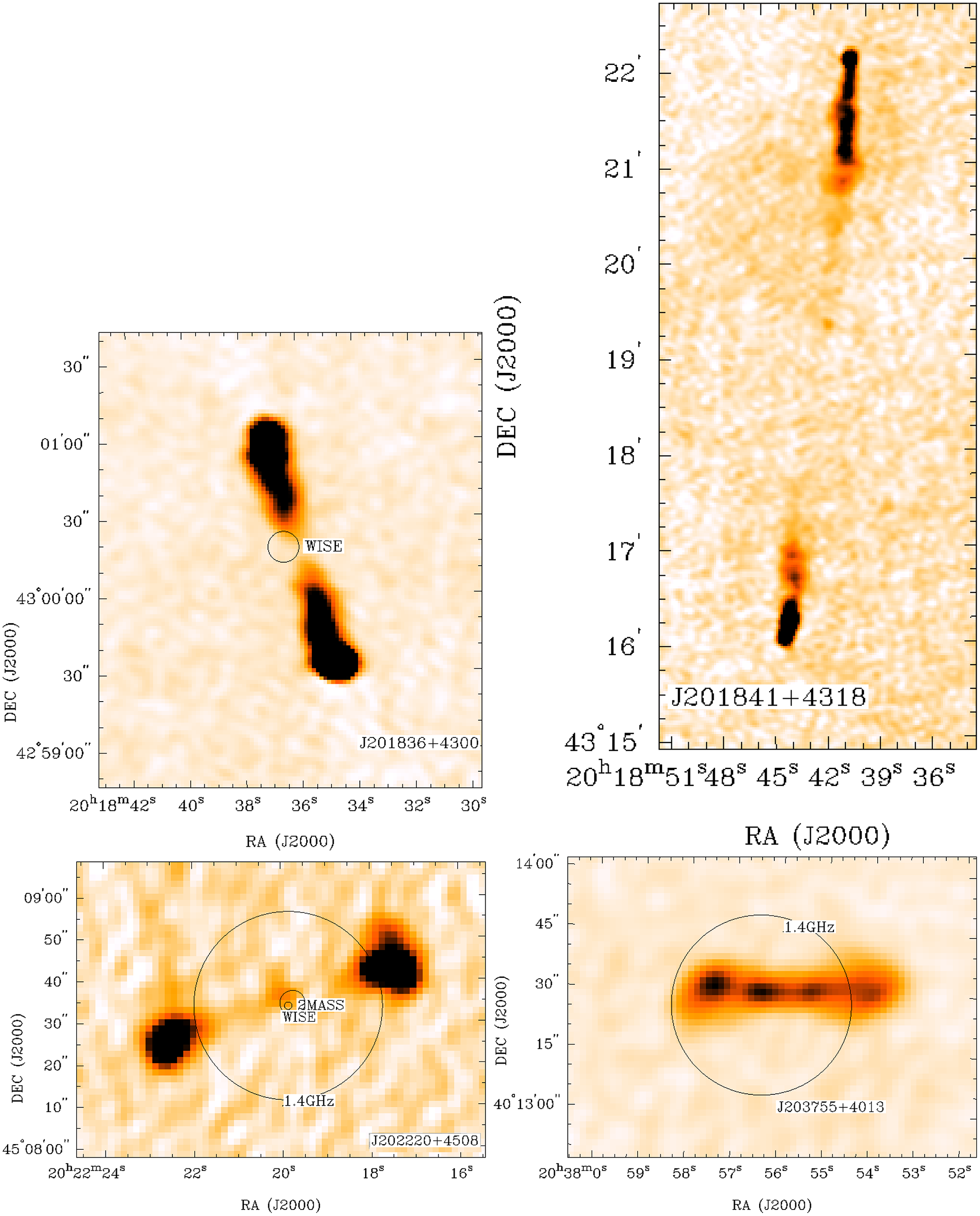
Spectral index (left) and error maps (right) of J201739+421252 (#4, first row), J201758+403100 (#5, second row), J202359+435525 (#15, third row), and J203345+404015 (#31, fourth row) sources. The synthesised beam is shown at the bottom left corner of each image.
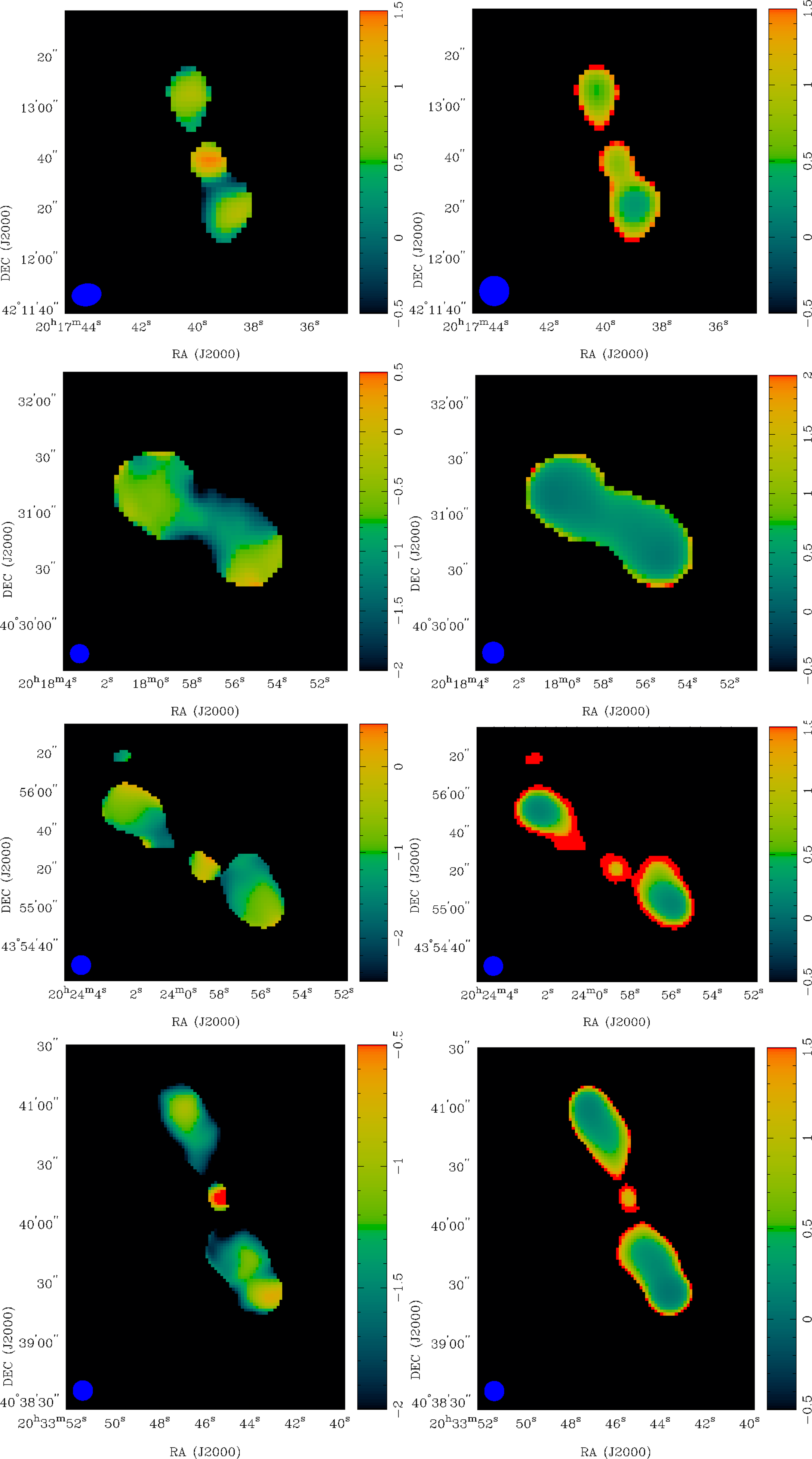
GMRT contours at 610 MHz (red) and 325 MHz (blue) overlaid on WISE (W1-band)/2MASS (3.4
 $\mu$
m) infrared images. The contour levels at 325 MHz are the same shown in Figures A1-A6. The contour levels at 610 MHz are: #10-J202151+423847:
$\mu$
m) infrared images. The contour levels at 325 MHz are the same shown in Figures A1-A6. The contour levels at 610 MHz are: #10-J202151+423847:
 $-2.5$
, 2.5, 3, and 5, in units of
$-2.5$
, 2.5, 3, and 5, in units of
 $\sigma(=0.13\,\mathrm{mJy\,beam}^{-1}$
). #15-J202352+435525:
$\sigma(=0.13\,\mathrm{mJy\,beam}^{-1}$
). #15-J202352+435525:
 $-2.5$
, 2.5, 5, 9, 15, 21, and 27, in units of
$-2.5$
, 2.5, 5, 9, 15, 21, and 27, in units of
 $\sigma(=0.1\,\mathrm{mJy\,beam}^{-1}$
). #16-J202403+413611:
$\sigma(=0.1\,\mathrm{mJy\,beam}^{-1}$
). #16-J202403+413611:
 $-2.5$
, 2.5, 5, and 15, in units of
$-2.5$
, 2.5, 5, and 15, in units of
 $\sigma(=0.15\,\mathrm{mJy\,beam}^{-1}$
). #21-J202632+412942:
$\sigma(=0.15\,\mathrm{mJy\,beam}^{-1}$
). #21-J202632+412942:
 $-2.5$
, 2.5, 5, 10, 15, 25, and 35, in units of
$-2.5$
, 2.5, 5, 10, 15, 25, and 35, in units of
 $\sigma(=0.1\,\mathrm{mJy\,beam}^{-1}$
). #22-J202645+431435:
$\sigma(=0.1\,\mathrm{mJy\,beam}^{-1}$
). #22-J202645+431435:
 $-2.5$
, 2.5, 5, 9, and 15, in units of
$-2.5$
, 2.5, 5, 9, and 15, in units of
 $\sigma(=0.1\,\mathrm{mJy\,beam}^{-1}$
). #24-J202755+423215:
$\sigma(=0.1\,\mathrm{mJy\,beam}^{-1}$
). #24-J202755+423215:
 $-2.5$
, 2.5, 30, 50, and 130, in units of
$-2.5$
, 2.5, 30, 50, and 130, in units of
 $\sigma(=0.1\,\mathrm{mJy\,beam}^{-1}$
). #26-J202859+402141:
$\sigma(=0.1\,\mathrm{mJy\,beam}^{-1}$
). #26-J202859+402141:
 $-2.5$
, 2.5, 9, 15, 21, and 27, in units of
$-2.5$
, 2.5, 9, 15, 21, and 27, in units of
 $\sigma(=0.1\,\mathrm{mJy\,beam}^{-1}$
). #31-J203345+404015:
$\sigma(=0.1\,\mathrm{mJy\,beam}^{-1}$
). #31-J203345+404015:
 $-2.5$
, 2.5, 9, 15, 21, and 27, in units of
$-2.5$
, 2.5, 9, 15, 21, and 27, in units of
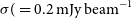 $\sigma(=0.2\,\mathrm{mJy\,beam}^{-1}$
). #32-J203402+420615:
$\sigma(=0.2\,\mathrm{mJy\,beam}^{-1}$
). #32-J203402+420615:
 $-2.5$
, 2.5, 9, 15, 21, and 27, in units of
$-2.5$
, 2.5, 9, 15, 21, and 27, in units of
 $\sigma(=0.1\,\mathrm{mJy\,beam}^{-1}$
). The synthesised beams are shown at the bottom left corner of each image.
$\sigma(=0.1\,\mathrm{mJy\,beam}^{-1}$
). The synthesised beams are shown at the bottom left corner of each image.
GMRT contours at 610 MHz (red) and 325 MHz (blue) overlaid on WISE/2MASS infrared images. The contour levels at 325 MHz are the same shown in Figures A1-A6. The contour levels at 610 MHz are: #35-J203431+413037:
 $-2.5$
, 2.5, 9, 15, 21, 35, and 55, in units of
$-2.5$
, 2.5, 9, 15, 21, 35, and 55, in units of
 $\sigma(=0.12\,\mathrm{mJy\,beam}^{-1}$
). #40-J201836+430018:
$\sigma(=0.12\,\mathrm{mJy\,beam}^{-1}$
). #40-J201836+430018:
 $-2.5$
, 2.5, 10, and 20, in units of
$-2.5$
, 2.5, 10, and 20, in units of
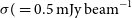 $\sigma(=0.5\,\mathrm{mJy\,beam}^{-1}$
). #42-J203431+413035:
$\sigma(=0.5\,\mathrm{mJy\,beam}^{-1}$
). #42-J203431+413035:
 $-2.5$
, 2.5, 5, 9, 15, 21, 35, 55, and 85, in units of
$-2.5$
, 2.5, 5, 9, 15, 21, 35, 55, and 85, in units of
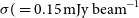 $\sigma(=0.15\,\mathrm{mJy\,beam}^{-1}$
). The synthesised beams are shown at the bottom left corner of each image.
$\sigma(=0.15\,\mathrm{mJy\,beam}^{-1}$
). The synthesised beams are shown at the bottom left corner of each image.