





Impact Statement
This work focuses on stretching numerical predictions to their practical limit for transonic fluid–structure interaction. Short wings, such as canards and control surfaces, are particularly sensitive to the development of vortical structures near the wing root, where the interaction between the wing and the supporting body can generate strong juncture vortices. These vortices may introduce unsteady aerodynamic loads and structural vibrations that are difficult to interpret experimentally. Without the support of coupled FSI simulations, such vibrations may be mistakenly attributed to parasitic frequencies from the wind-tunnel model, support system, or facility components.
This work shows that high-fidelity numerical simulations, when carefully validated against experiments, can help distinguish genuine aeroelastic mechanisms from facility- or model-related artefacts. The results therefore provide useful guidance for interpreting wind-tunnel measurements, improving numerical modelling strategies, and assessing the aeroelastic behaviour of compact lifting surfaces operating in transonic flow.
1. Introduction
Transonic fluid–structure interactions (FSIs) are an extremely challenging field of research because of the inherently three-dimensional, unsteady pressure fluctuations induced by the interplay between shock waves and the separation region (Davis Reference Davis and O.1993; Denegri Reference Denegri2000; Foughner & Besinger Reference Foughner and Besinger1977). Typically, the aerodynamic loading varies nonlinearly with Mach number and amplitude of deformation, thus reducing the accuracy of low-fidelity and reduced-order models. The renewed interest in civil aeroplanes with high-aspect-ratio wings requires accurate aeroelastic predictions, often including the whole fuselage effect in the final analysis (Gray et al. Reference Gray2023; Riso & Cesnik Reference Riso and Cesnik2023). In addition, crossflows due to unevenly distributed separation regions (Illi et al. Reference Illi, Fingskes, Lutz and Kramer2013; Poplingher & Raveh Reference Poplingher and Raveh2023) and boundary-layer transition (Wang et al. Reference Wang, Xu, Zhang and Bai2023) further reduce the predictive capability of reduced-order models, to the point where both experiments and high-performance computing are required to simulate FSIs.
An important aspect in transonics and high-speed subsonics is the presence of free vortices. Deep-stall lock-in induced by free-shear-layer/horizontal-stabilizer interactions (Glazkov et al. Reference Glazkov, Gorbushin, Khoziaenko, Konotop and Terekhin2005) was historically one of the main challenges in crossing the sound barrier, and it is the reason why early supersonic aircraft generally employed a T-tail with a high-mounted stabiliser (Anderson and Cadou, Reference Anderson and Cadou2024, Chapter 11, pp. 751–822). In this context, the present work focuses on vortex-induced disturbances generated by localised geometrical changes such as body–wing or truss–wing junctions in large-aspect-ratio wings. The work of Gur et al. (Reference Gur, Bhatia, Schetz, Mason, Kapania and Mavris2012) presents a global study of such configurations in the transonic regime, showing that juncture interference contributes between approximately 2 % and 10 % of the total drag when appropriate fairing is employed.
Because of their relative size, the effect of juncture vortices is further enhanced for wings with small aspect ratio. This behaviour can also be observed in other aerodynamic components, such as high hub-to-tip ratio compressor blades, which can be very short and are therefore strongly affected by the boundary layer developing on both the hub and the cowl (Saravanamuttoo et al. Reference Saravanamuttoo, Rogers and Cohen2001). Similarly, for canards and short all-movable wings, vortex-induced pressure variations can affect a large portion of the suction side. At high speeds, this becomes particularly critical because canards are positioned close to the nose; therefore, small variations in deflection or pressure can produce large changes in aerodynamic moment (Ghoreyshi et al. Reference Ghoreyshi, R.Darragh, Lofthouse, A. and Hamlingtonc2017). In experimental settings, additional complexities arise: wall-mounted wings typically suffer from the boundary layer developing along the test-section walls, leading to vortex formation between the model and the wall, while sting-mounted configurations can alter fuselage–wing interactions. Consequently, careful design of the mounting system and test-section conditions is required (Coustols et al. Reference Coustols, Seraudie and Mignosi1997; Glazkov et al. Reference Glazkov, Gorbushin, Khoziaenko, Konotop and Terekhin2005).
Despite their importance, modelling of juncture and tip vortices in transonics remains limited. One of the few exceptions is the work of Lyrintzis & Xue (Reference Lyrintzis and Xue1991), where tip vortices were modelled using a two-dimensional theory with corrections for three-dimensional effects via the Kirchhoff method. However, this approach assumes a filament vortex aligned with the wing-span direction. In contrast, juncture vortices are typically described as horseshoe vortices convecting downstream (Simpson Reference Simpson2001). Classical models, such as Widnall’s theory for helical instability (Widnall Reference Tsai and Widnall1975) and Batchelor’s model for vortex decay and breakdown (Delbende et al. Reference Delbende, Chomaz and Huerre1998), provide useful insight into vortex dynamics. In transonics, vortices in the immediate vicinity of the wall are known to contribute significantly to vibration and buffet, suggesting that Widnall-type mechanisms may play a dominant role. According to this framework, the filament vortex motion arises from a linearisation of the Euler equations, and the lowest instability frequency is typically of the order of $(0.25 {-} 0.33)\varGamma /(2\pi r)$
, where
$(0.25 {-} 0.33)\varGamma /(2\pi r)$
, where $\varGamma$
is the circulation and
$\varGamma$
is the circulation and $r$
the vortex core radius (Widnall et al. Reference Widnall, Bliss and Tsai1974).
$r$
the vortex core radius (Widnall et al. Reference Widnall, Bliss and Tsai1974).
From an aeroelastic perspective, even relatively small angles of attack in transonic flow can generate vortices and large unsteady separation regions. The resulting aerodynamic loads are highly nonlinear and can induce significant structural deformations. For configurations with limited vibration amplitudes, such as short compressor blades, the aerodynamic response can be approximated as the superposition of a steady baseline and a transient component (Tateishi et al. Reference Tateishi, Watanabe, Himeno and Inoue2014). However, this small-perturbation approach breaks down in the presence of stall and large separation regions, due to the strongly nonlinear nature of transonic FSIs (Dowell Reference Dowell2022).
From a modelling standpoint, reduced-order and low-fidelity approaches remain attractive due to the high computational cost of fully resolved simulations. Generating high-quality meshes for three-dimensional geometries is time-consuming and often leads to highly stretched cells near walls and trailing edges, necessitating frequent remeshing in FSI simulations. Recent developments, such as the Volterra-series-based reduced-order model proposed by Candon et al. (Reference Candon, Delgado-Gutiérrez, Marzocca, Balajewicz and Dowell2025), show promising reductions in training requirements. However, such approaches are currently limited to low-incidence, small-amplitude oscillations. At present, no comprehensive reduced-order model is capable of accurately predicting near- and post-stall FSIs in transonic regimes.
In this context, the present work aims to address this gap by providing a combined numerical and experimental investigation of a free-to-pitch wing (aspect ratio $AR = 1.54$
) operating in deep stall under transonic conditions. The experimental set-up is described in § 2, while numerical methods and mesh details are presented in § 3. Steady numerical characterisation, FSI simulations and comparison with experimental results are discussed in § 4, followed by conclusions in § 7.
$AR = 1.54$
) operating in deep stall under transonic conditions. The experimental set-up is described in § 2, while numerical methods and mesh details are presented in § 3. Steady numerical characterisation, FSI simulations and comparison with experimental results are discussed in § 4, followed by conclusions in § 7.
2. Experimental set-up
2.1. Wind tunnel description
The transonic wind tunnel is located at the Aerospace Science and Technology Research Center (ASTRC) of the National Cheng Kung University (NCKU). Details about the facilities can be found in Chung et al. (Reference Chung, Miau and Yieh1994) and Currao (Reference Currao2024). The test section has a square frontal area with 600 mm long edges and a length of 1.5 m, and need to be included in the numerical modelling. The flow is established within a few seconds, thus providing about 6 s of flow. Stagnation temperature can be considered equal to room temperature, as a thermal mass matrix upstream of the wind tunnel nozzle allows for a maximum drop smaller than 10 K during 30 s of test time. As shown in a previous related work (see Currao (Reference Currao2024), figure 1b), free-stream noise produces free-stream pressure fluctuations of up to 10 % during the test. With the nozzle and settings used in this framework, the nominal free-stream conditions are $M_\infty = 0.77$
,
$M_\infty = 0.77$
, $p_\infty =116\,196$
Pa and
$p_\infty =116\,196$
Pa and $Re_\infty = 22.33 \times 10^6$
m
$Re_\infty = 22.33 \times 10^6$
m $^{-1}$
.
$^{-1}$
.
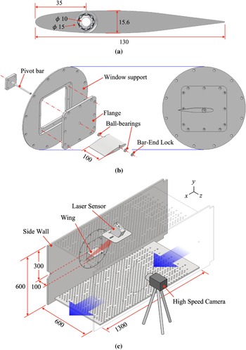
Technical drawings of the model within the wind tunnel (size in mm).

2.2. Wind tunnel model
As shown in figure 1, the wind tunnel model consists of a free-to-pitch symmetric rectangular wing positioned on the sidewall of the test section. The aerofoil employed is the NASA-(SC)2-0012. The maximum aerofoil thickness is 15.6 mm, while the chord and span measure 130 and 100 mm, respectively. The entire model is 3D-printed with carbon-fiber-infused nylon (PA-CF), with a nominal Young’s modulus of 2.7 GPa and a density of 1.15 g cm−3. During the 3D-printing process, approximately $90\,\%$
of the internal volume was filled resulting in a virtually underformable wing model. At 35 mm from the leading edge, the wing presents a horizontal orifice that allows for the pivot-bar positioning. The wing and bar are connected through two ball bearings to minimise friction. The weight of the model, including the ball bearings, is
$90\,\%$
of the internal volume was filled resulting in a virtually underformable wing model. At 35 mm from the leading edge, the wing presents a horizontal orifice that allows for the pivot-bar positioning. The wing and bar are connected through two ball bearings to minimise friction. The weight of the model, including the ball bearings, is $m = 68.9$
g while the the inertia of the model around the pivot is
$m = 68.9$
g while the the inertia of the model around the pivot is $I = 6.7337\times 10^{-5}$
kg m2. The dynamics of the wing can be modelled as follows:
$I = 6.7337\times 10^{-5}$
kg m2. The dynamics of the wing can be modelled as follows:
 \begin{equation} I\ddot {\alpha } + D\dot {\alpha } = M_y(\alpha ,\dot {\alpha },t) + mge\sin (\alpha ). \end{equation}
Here, $M_y$
represents the aerodynamic moment, which depends on the instantaneous wing inclination and transient hysteretic phenomena, and
$M_y$
represents the aerodynamic moment, which depends on the instantaneous wing inclination and transient hysteretic phenomena, and $\alpha$
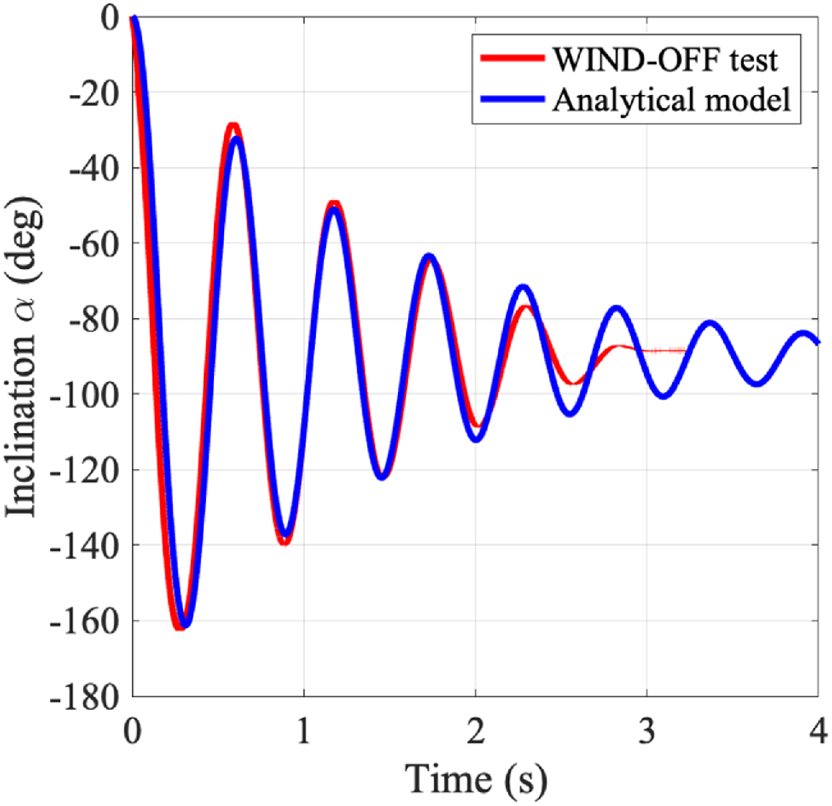
represents both the wing pitch (rotation) angle and the angle of attack. Since the aerofoil profile is symmetric, these two quantities are equivalent in the present study, and the same definition is used consistently throughout the paper. Through a free-oscillation test, it is possible to evaluate the missing parameters, namely the damping
$\alpha$
represents both the wing pitch (rotation) angle and the angle of attack. Since the aerofoil profile is symmetric, these two quantities are equivalent in the present study, and the same definition is used consistently throughout the paper. Through a free-oscillation test, it is possible to evaluate the missing parameters, namely the damping $D$
and the eccentricity
$D$
and the eccentricity $e$
. The wing is released from an initial position of
$e$
. The wing is released from an initial position of $\alpha = 0^\circ$
and allowed to oscillate freely. Because the centre of mass is located behind the pivot, the wing naturally oscillates around a pitch-up equilibrium position of approximately
$\alpha = 0^\circ$
and allowed to oscillate freely. Because the centre of mass is located behind the pivot, the wing naturally oscillates around a pitch-up equilibrium position of approximately $90^\circ$
, corresponding to a vertical orientation of the wing with the leading edge pointing upward, as shown in figure 3. It was possible to locate the centre of mass at 57.7 mm from the leading edge, with an accuracy of
$90^\circ$
, corresponding to a vertical orientation of the wing with the leading edge pointing upward, as shown in figure 3. It was possible to locate the centre of mass at 57.7 mm from the leading edge, with an accuracy of $\pm 2.5\,\%$
, and a damping coefficient of
$\pm 2.5\,\%$
, and a damping coefficient of $D = 10^{-6}$
N m s−1. In terms of the Rayleigh formulation, this can be expressed as
$D = 10^{-6}$
N m s−1. In terms of the Rayleigh formulation, this can be expressed as $D = I \alpha _R$
, where the Rayleigh mass coefficient is
$D = I \alpha _R$
, where the Rayleigh mass coefficient is $\alpha _R = 1.485 \times 10^{-2}$
(Liu & Gorman Reference Liu and Gorman1995).
$\alpha _R = 1.485 \times 10^{-2}$
(Liu & Gorman Reference Liu and Gorman1995).
It can be demonstrated, however, that due to the very low weight of the model, the actual distance $e$
between the pivot and the centre of mass – and thus the second term on the right-hand side of the equation – can be considered negligible during a wind-on test. The solution is also relatively unaffected by damping variations of less than one order of magnitude. The maximum moment induced by the weight about the pivot is approximately 0.015 N m, which is less than
$e$
between the pivot and the centre of mass – and thus the second term on the right-hand side of the equation – can be considered negligible during a wind-on test. The solution is also relatively unaffected by damping variations of less than one order of magnitude. The maximum moment induced by the weight about the pivot is approximately 0.015 N m, which is less than $1\,\%$
of the maximum aerodynamic moment (approximately 2 N m near stall). For this reason, the weight of the wing is included in the simulations for completeness, but it does not significantly affect the FSIs.
$1\,\%$
of the maximum aerodynamic moment (approximately 2 N m near stall). For this reason, the weight of the wing is included in the simulations for completeness, but it does not significantly affect the FSIs.
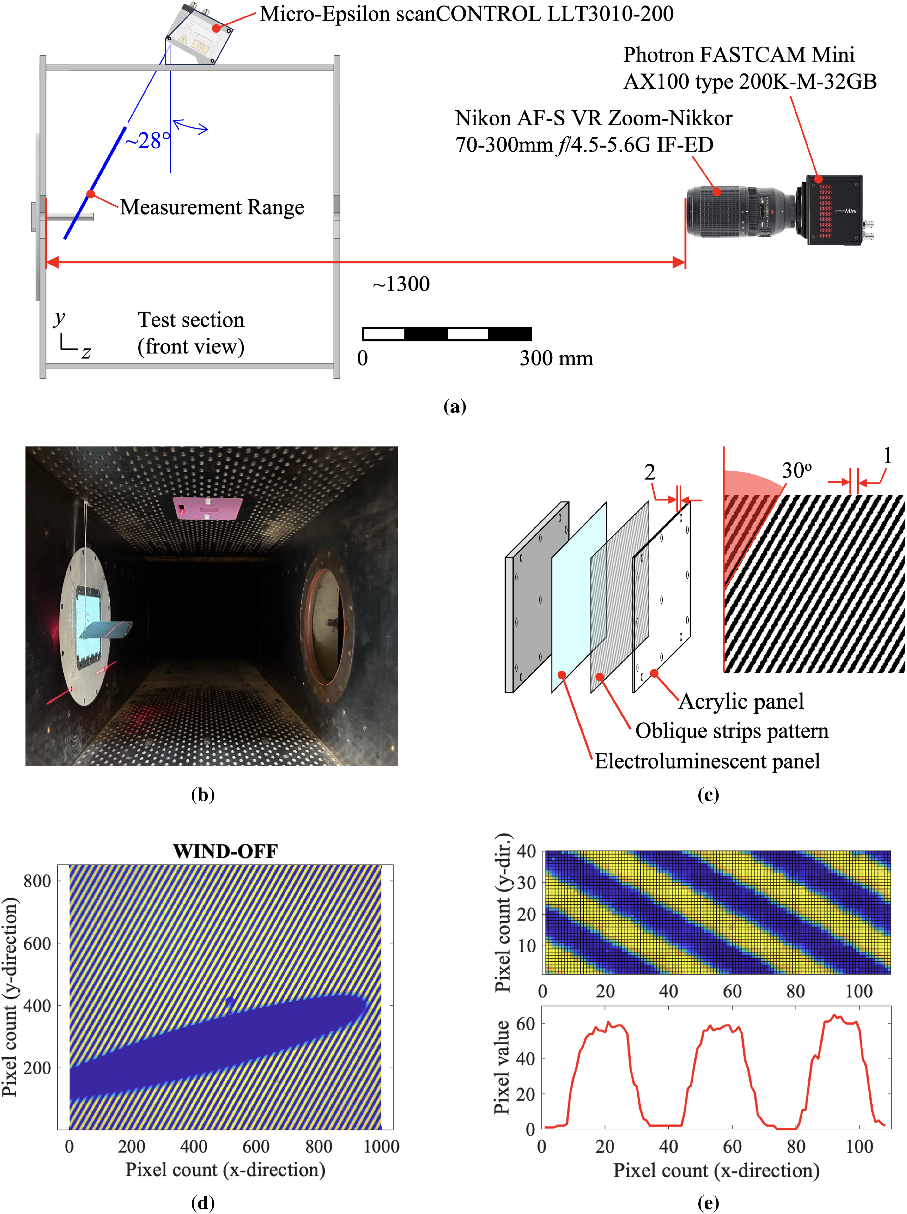
Details of the BOS set-up: (a) positioning, (b) test section, (c) luminescent background and (d, e) pixel intensity distribution.
As for the experiment, just before the test the wing is held at a positive initial angle of attack using a paper clip, as shown in figure 2(d). During the initial transient, the paper clip holding the wing is blown away and the wing starts oscillating under the effect of the flow.
Comparison between bench test and analytical model to isolate centre of mass and damping.
2.3. Instrumentation
The model dynamics is measured through two different means, namely a laser scanner and a high-speed camera. Referring to figure 2(a, b), the laser scanner (Micro-Epsilon scanCONTROL LLT3010-200) is used to measure the oscillation frequency. The maximum sampling frequency is 10 kHz, and the displacement accuracy is of the order of 10 μm. However, the sampling frequency is reduced to 3429 Hz to keep the number of query points on the wing above 50. Additionally, sampling frequencies greater than 4 kHz cannot be considered due to limitations in the size of the sampling region. Since the test section offers only one porthole in the middle of the top bleeding wall, it is necessary to incline the laser by approximately $30^\circ$
to measure the wing motion. Consequently, the query points are distributed not only along the chord but also along the span of the wing. For this reason, it is difficult to perform accurate inclination measurements when the model is oscillating. Therefore, the laser data are presented mainly in terms of power spectral density (PSD) of the displacement measurements. As will be discussed, frequency measurements are also affected by wind tunnel vibrations with a frequency of 50–100 Hz, since the laser scanner is mounted on the top wall of the test section. Thus, in addition to laser-based measurements, high-speed camera measurements are also performed from outside the wind tunnel in order to better interpret the laser data.
$30^\circ$
to measure the wing motion. Consequently, the query points are distributed not only along the chord but also along the span of the wing. For this reason, it is difficult to perform accurate inclination measurements when the model is oscillating. Therefore, the laser data are presented mainly in terms of power spectral density (PSD) of the displacement measurements. As will be discussed, frequency measurements are also affected by wind tunnel vibrations with a frequency of 50–100 Hz, since the laser scanner is mounted on the top wall of the test section. Thus, in addition to laser-based measurements, high-speed camera measurements are also performed from outside the wind tunnel in order to better interpret the laser data.
The high-speed camera (FASTCAM Mini AX100) is used to perform both inclination measurements and background-oriented schlieren (BOS) visualisation; thus, two different set-ups are employed depending on the type of analysis. High-frequency oscillations are measured using a generic lens, a Sigma 85 mm F1.4 EX DG HS, and a frame rate of 6 kHz. This allows for a small window around the object of $640 \times 640$
pixels, with a resolution of approximately 0.32 mm pixel−1. When BOS visualisation is performed, it is necessary to have increased resolution and a high signal-to-noise ratio (SNR). In this case, a lens with a longer focal length (300 mm) is used – namely, a Nikon AF-S VR Zoom-Nikkor 70-300 mm f/4.5–5.6G IF-ED (aperture = f/5.6). To increase the SNR, the frame rate is reduced to 1 kHz. This enables a maximum variation of approximately 60 pixel intensity levels between the darkest and brightest regions, as shown in figure 2(d, e). The window of interest remains
$640 \times 640$
pixels, with a resolution of approximately 0.32 mm pixel−1. When BOS visualisation is performed, it is necessary to have increased resolution and a high signal-to-noise ratio (SNR). In this case, a lens with a longer focal length (300 mm) is used – namely, a Nikon AF-S VR Zoom-Nikkor 70-300 mm f/4.5–5.6G IF-ED (aperture = f/5.6). To increase the SNR, the frame rate is reduced to 1 kHz. This enables a maximum variation of approximately 60 pixel intensity levels between the darkest and brightest regions, as shown in figure 2(d, e). The window of interest remains $640 \times 640$
pixels but is focused on the forepart of the wing, resulting in an increased resolution of 0.12 mm pixel−1.
$640 \times 640$
pixels but is focused on the forepart of the wing, resulting in an increased resolution of 0.12 mm pixel−1.
2.4. Background-oriented schlieren
The BOS system is a relatively inexpensive, compact and simple method to measure flow structures when classical schlieren or shadowgraph methods are not available (Mercier & Lacassagne Reference Mercier and Lacassagne2023; Raffel et al. Reference Raffel, Richard and Meier2000). As shown in figure 2, it is necessary to create a speckled or spangled background; the latter is chosen here, as it leads to a higher SNR. During the test, variations in flow density lead to changes in the refractive index; consequently, the recorded position of the stripes on the background is altered. Through post-processing, it is possible to track recurring features between two recorded images, thereby enabling visualisation of strong density variations. However, BOS is negatively affected by the background intensity and the physical distance between the background and the object.
To increase the contrast between the background stripes – and consequently the sharpness of the post-processed images – the background is printed on a very thin paper sheet and glued onto an electroluminescent panel (see figure 2 c). As mentioned above, a maximum resolution of 60 intensity levels was achieved under optimal conditions (see figure 2 d, e). This resolution is sufficient to visualise normal shocks on the wing suction side, but it is barely adequate for visualising shear layers and boundary layers. Additionally, the electroluminescent panel intensity fluctuates continuously at a frequency of 400 Hz, which slightly degrades image quality and interferes with frequency measurements. The greatest limitation of this technique is that, due to the limited size of the test section, the distance between the background and the model is very small (around 100 mm), while the distance between the camera and the model is significantly larger (1.3 m). Ideally, the distances between the camera, object and background should all be large so that the camera can focus on both the object and the background simultaneously. The best results are indeed obtained for flow visualisations around flying objects that use the ground or sky as a background (Raffel et al. Reference Raffel, Heineck, Schairer, Leopold and Kindler2014). However, during wind tunnel tests, focusing on the background reduces the sensitivity of BOS to density variations along the span of the model. To mitigate this effect, it is important to reduce the capture area as much as possible, to increase the focal length and carefully tune the camera aperture. A smaller aperture (i.e. a larger f-number) increases the depth of field, allowing both the model and the background to remain in focus. A large focal length is necessary because the distance between the model and the background is relatively small. For the experiments presented here, we used a focal length of 300 mm and an aperture of f/5.6.
The post-processing of the recorded images is performed using a MATLAB application called comBOS. As explained in more detail by Mercier and Lacassagne (Reference Mercier and Lacassagne2023), the algorithm can be simplified as follows. Let us assume the intensity distributions of two consecutive frames are $f(x,y)$
and
$f(x,y)$
and $g(x,y)$
. A feature in the second frame may be a shifted version of a feature in the first frame, possibly with a different intensity value. Thus, for every pixel, it is possible to write the following equation:
$g(x,y)$
. A feature in the second frame may be a shifted version of a feature in the first frame, possibly with a different intensity value. Thus, for every pixel, it is possible to write the following equation:
 \begin{equation} af(x_i,y_i)+b=g(x_i+\Delta x,y_i+\Delta y), \end{equation}
where $a$
and
$a$
and $b$
are constants while
$b$
are constants while $\Delta x$
,
$\Delta x$
, $\Delta y$
represent the shift. By using the chain rule to expand
$\Delta y$
represent the shift. By using the chain rule to expand $g$
, for every ith pixel it is possible to write the following relation:
$g$
, for every ith pixel it is possible to write the following relation:
 \begin{equation} af_i+b - g_i - \frac {\partial g_i}{\partial x}\Delta x - \frac {\partial g_i}{\partial y}\Delta y = 0, \end{equation}
where $f_i =f(x_i,y_i)$
and
$f_i =f(x_i,y_i)$
and $g_i=g(x_i,y_i)$
. However, this formulation assumes that every feature in the first frame is shifted uniformly by
$g_i=g(x_i,y_i)$
. However, this formulation assumes that every feature in the first frame is shifted uniformly by $\Delta x$
and
$\Delta x$
and $\Delta y$
, which is generally not true. Nonetheless, within a sufficiently small domain, the shift can be approximated as locally constant and uniform. Typically, this subdomain contains between 6 and 12 pixels, which inevitably reduces the effective resolution. Equation (2.3) can be built for every pixel in the subdomain, resulting in an overdetermined system of algebraic equations with only four unknowns:
$\Delta y$
, which is generally not true. Nonetheless, within a sufficiently small domain, the shift can be approximated as locally constant and uniform. Typically, this subdomain contains between 6 and 12 pixels, which inevitably reduces the effective resolution. Equation (2.3) can be built for every pixel in the subdomain, resulting in an overdetermined system of algebraic equations with only four unknowns: $\Delta x$
,
$\Delta x$
, $\Delta y$
,
$\Delta y$
, $a$
and
$a$
and $b$
. For every subdomain of
$b$
. For every subdomain of $n$
pixels, the system of equations can be written as
$n$
pixels, the system of equations can be written as
 \begin{equation} \left [ \begin{array}{cccc} \dfrac {\partial g_1}{\partial x} &\quad \dfrac {\partial g_1}{\partial y} &\quad -f_1&\quad -1\\[9pt] \dfrac {\partial g_2}{\partial x} &\quad \dfrac {\partial g_2}{\partial y} &\quad -f_2&\quad -1\\ \ldots & & & \\[6pt] \dfrac {\partial g_n}{\partial x} &\quad \dfrac {\partial g_n}{\partial y} &\quad -f_n &\quad -1\\ \end{array} \right ] \left \{ \begin{array}{c} \Delta x\\[3pt] \Delta y\\[3pt] a\\[3pt] b\\ \end{array}\right \}= \left [ \begin{array}{c} -g_1\\[3pt] -g_2\\[3pt] \ldots \\[3pt] -g_n\\ \end{array} \right ]. \end{equation}
The solution to this system is the one that minimises the residual, i.e. the least-squares solution. Given the nature of the problem, it was discovered that the shift in the y direction is relatively small and thus the total shift $\sqrt {\Delta x^2 + \Delta y^2}\simeq \Delta x$
.
$\sqrt {\Delta x^2 + \Delta y^2}\simeq \Delta x$
.
Detailed view of (a) numerical domain and (b–e) meshed sidewall.

3. Numerical technique
The commercial software ANSYS Fluent was used to solve the three-dimensional, unsteady Reynolds-averaged Navier–Stokes (RANS) equations and to perform detached-eddy simulations (DES). The governing equations and turbulence models are implemented within the solver and are therefore not repeated here for brevity; the reader is referred to the ANSYS Fluent Theory Guide for a complete formulation. The flow was modelled assuming a compressible, ideal gas. Adiabatic wall boundary conditions were applied ( $q_w = 0$
). Turbulence effects were accounted for by using the
$q_w = 0$
). Turbulence effects were accounted for by using the $k$
–
$k$
– $\omega$
shear-stress transport (SST) model (Menter 1994), selected for its robustness in both boundary layers and separated shear flows. In DES mode, the SST model was combined with a DES formulation following Menter et al. (Reference Menter, Kuntz and Langtry2003), where the turbulence length scale is modified based on the local grid spacing. The simulations were performed using an implicit, density-based solver with second-order spatial discretisation. Temporal integration was carried out using a second-order implicit scheme. All convective terms were discretised using a second-order upwind scheme.
$\omega$
shear-stress transport (SST) model (Menter 1994), selected for its robustness in both boundary layers and separated shear flows. In DES mode, the SST model was combined with a DES formulation following Menter et al. (Reference Menter, Kuntz and Langtry2003), where the turbulence length scale is modified based on the local grid spacing. The simulations were performed using an implicit, density-based solver with second-order spatial discretisation. Temporal integration was carried out using a second-order implicit scheme. All convective terms were discretised using a second-order upwind scheme.
Detailed view of the meshed wing surface.

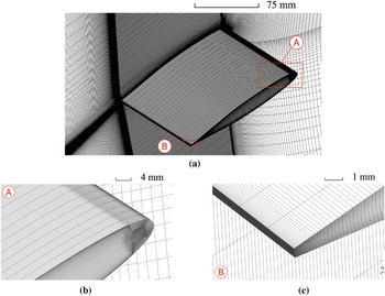
Mesh details are given in figures 4 and 5. The fluid domain has a cell count of approximately 15 millions. The mesh was created manually using the blocking strategy, which allows sharing mesh parameters between parallel edges of different mesh blocks. Near the wall, it is necessary to reach a minimum cell height of approximately 5 μm in order to have $y^{+}\lt 1$
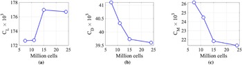
with 3–5 cells within the laminar sublayer. Unfortunately, typical cell length and width near the wall are of the order of 2 mm to maintain the total cell count within acceptable limits. This results in average cell aspect ratio close to 400 in the vicinity of the wall. While for rigid (i.e. no moving structure) simulations this is not a concern, FSI simulations significantly suffer from high-aspect-ratio cells – especially at the start (or restart) of the simulation, when reference residuals are normally calculated. In such cases, the simulation can immediately fail due to the formation of negative-volume cells. The only way to solve this problem is to decrease the mesh size near the wall to approximately 0.5 mm, thus resulting in an over-refined mesh with more than 25 million cells, as shown in the mesh independence study in figure 6.
$y^{+}\lt 1$
with 3–5 cells within the laminar sublayer. Unfortunately, typical cell length and width near the wall are of the order of 2 mm to maintain the total cell count within acceptable limits. This results in average cell aspect ratio close to 400 in the vicinity of the wall. While for rigid (i.e. no moving structure) simulations this is not a concern, FSI simulations significantly suffer from high-aspect-ratio cells – especially at the start (or restart) of the simulation, when reference residuals are normally calculated. In such cases, the simulation can immediately fail due to the formation of negative-volume cells. The only way to solve this problem is to decrease the mesh size near the wall to approximately 0.5 mm, thus resulting in an over-refined mesh with more than 25 million cells, as shown in the mesh independence study in figure 6.
Mesh deformation in the FSI simulations was handled using the smoothing method implemented in the solver. The diffusion function was set to boundary distance so that mesh deformation decayed progressively away from the moving surface. A diffusion parameter between 1 and 2 was used to balance mesh adaptability near the wing with stability in the outer mesh. The pitch amplitude itself did not pose a significant problem for the mesh deformation; however, modelling the initial transient – i.e. the transition of the wing from the initial angle of attack to the equilibrium position – can result in mesh failure because the deformation occurs too rapidly. This is the reason why FSI simulations were initialised with angle of attack close to equilibrium ( $\alpha \sim 10^\circ {-} 12^\circ$
).
$\alpha \sim 10^\circ {-} 12^\circ$
).
Mesh independence study (steady simulations, angle of attack = $\textit{6}^\circ$
).
$\textit{6}^\circ$
).

In the case of FORERUNNER1 – the Taiwanese HPC platform used to produce this work – the optimal cell distribution was found to be approximately 11 cores per million cells. If a simulation is run on a single 112-core node, the ideal mesh should not exceed 10 million cells. Under these settings, approximately 10 FSI time steps are computed every hour (equivalent to 0.09 iterations per CPU).
Structure FEM solver mesh and geometrical details.

To further reduce the computational burden, the body is simplified as a group or rigid surfaces so as to avoid meshing the internal part of the body. As shown in figure 7, the structure mesh is extracted from the CFD domain such that each structural cell node is coincident with the corresponding fluid cell node, promoting a fast exchange between the FEM and CFD solvers in terms of nodal displacement and loads. In order to reproduce the actual position of the centre of gravity, a so-called mass bar with the same mass as the model is located at 48.4 mm from the leading edge. At 35 mm from the leading edge, two concentric cylinders are included to simulate the pitch-only constraint.
Time independence study.

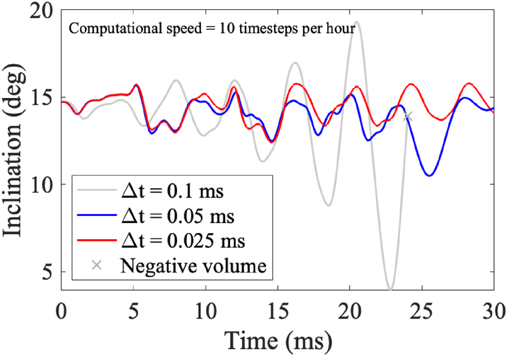
The time necessary for a flow disturbance to travel a distance equal to two times the chord of the aerofoil is approximately $1$
ms. Figure 8 shows that, if a time step
$1$
ms. Figure 8 shows that, if a time step $\Delta t = 0.1$
ms is chosen, the aeroelastic response enters a post-flutter regime characterised by oscillations of progressively increasing amplitude rather than converging to a limit-cycle oscillation, with the solver failing at about
$\Delta t = 0.1$
ms is chosen, the aeroelastic response enters a post-flutter regime characterised by oscillations of progressively increasing amplitude rather than converging to a limit-cycle oscillation, with the solver failing at about $25$
ms due to its inability to cope with large mesh deformations. The chosen time step is
$25$
ms due to its inability to cope with large mesh deformations. The chosen time step is $\Delta t = 0.025$
ms. As can be seen from the figure, the discrepancy between
$\Delta t = 0.025$
ms. As can be seen from the figure, the discrepancy between $\Delta t = 0.05$
and
$\Delta t = 0.05$
and $0.025$
ms is actually very small for the first
$0.025$
ms is actually very small for the first $10$
ms, and it becomes more significant due to the accumulation of error.
$10$
ms, and it becomes more significant due to the accumulation of error.
The supercomputing platform imposes a maximum wall-clock runtime of four days, requiring long simulations to be periodically restarted. In simulations involving a deforming mesh, grid quality progressively deteriorates as the oscillatory motion accumulates over time, and mesh residuals are often reset during restart. Consequently, restarting from the most recent time step is not always possible, and the computation may need to resume from an earlier checkpoint. In practice, after approximately 20 oscillation cycles the mesh quality typically deteriorates to the point where continuing or restarting the simulation is no longer feasible without intervention.
Static characterisation: aerodynamic moment around the pivot (quarter-chord position) from both steady RANS simulation and transient DES.

Aerodynamic characteristics before stall. Comparison between theory and steady simulations in terms of: (a) moment slope $\partial C_M/\partial \alpha$
around the pivot, (b) lift slope
$\partial C_M/\partial \alpha$
around the pivot, (b) lift slope $\partial C_L/\partial \alpha$
and (c) location of the centre of pressure
$\partial C_L/\partial \alpha$
and (c) location of the centre of pressure $x_{CP}$
.
$x_{CP}$
.

4. Results
4.1. Static characterisation
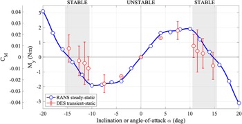
Figure 9 shows how the aerodynamic moment around the pivot changes with the wing inclination. Referring to the steady data points evaluated with the RANS model, the aerodynamic moment is zero at zero inclination and at an angle of attack of $\pm 14.7^\circ$
. Only the latter constitute stable equilibrium points, as the moment slope is negative. Near the stable equilibrium point, the DES reveal large variations in aerodynamic moment. Despite the overall agreement between steady and transient simulations, a well-defined equilibrium point cannot be clearly identified. The uncertainty in the stable equilibrium location is approximately
$\pm 14.7^\circ$
. Only the latter constitute stable equilibrium points, as the moment slope is negative. Near the stable equilibrium point, the DES reveal large variations in aerodynamic moment. Despite the overall agreement between steady and transient simulations, a well-defined equilibrium point cannot be clearly identified. The uncertainty in the stable equilibrium location is approximately $\pm 2.5^\circ$
.
$\pm 2.5^\circ$
.
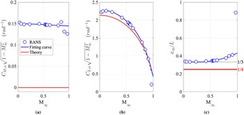
In order to verify the numerical results, it is important to also analyse the behaviour around the unstable point at zero incidence. Figures 10(a) and 10(b) show moment and lift slope – respectively $C_{M,\alpha } = \partial C_M / \partial \alpha$
and
$C_{M,\alpha } = \partial C_M / \partial \alpha$
and $C_{L,\alpha } = \partial C_L / \partial \alpha$
– multiplied by the Prandtl correction factor
$C_{L,\alpha } = \partial C_L / \partial \alpha$
– multiplied by the Prandtl correction factor $\sqrt {1 - M_\infty ^2}$
. Up to approximately
$\sqrt {1 - M_\infty ^2}$
. Up to approximately $M_\infty \simeq 0.75$
, the moment is nearly constant but not zero, because the centre of pressure is not located at the quarter-chord but closer to the one-third-chord location. According to (Anderson & Cadou Reference Anderson and Cadou2024, Chapter 11, pp. 751–822), the theoretical lift coefficient with corrections for a rectangular wing can be expressed as
$M_\infty \simeq 0.75$
, the moment is nearly constant but not zero, because the centre of pressure is not located at the quarter-chord but closer to the one-third-chord location. According to (Anderson & Cadou Reference Anderson and Cadou2024, Chapter 11, pp. 751–822), the theoretical lift coefficient with corrections for a rectangular wing can be expressed as
 \begin{equation} C_{L,\alpha } = \frac {c_{L}}{\sqrt {1 + \frac {c_{L}}{\pi AR} + \left (\frac {c_{L}}{\pi AR}\right )^2}}, \end{equation}
where the aspect ratio is $AR = 1.5385$
and the incompressible lift slope from thin aerofoil theory is
$AR = 1.5385$
and the incompressible lift slope from thin aerofoil theory is $c_{L} = 2\pi$
. The agreement between theory and simulation in figure 10(b) is good up to sonic conditions. Given both lift and moment, it is possible to estimate the centre of pressure to be located at approximately one-third of the chord, as shown in figure 10(c).
$c_{L} = 2\pi$
. The agreement between theory and simulation in figure 10(b) is good up to sonic conditions. Given both lift and moment, it is possible to estimate the centre of pressure to be located at approximately one-third of the chord, as shown in figure 10(c).
Static characterisation: Mach number distribution at different span locations from steady-static RANS simulations.

Figure 11 shows the Mach number distribution around the wing at different spanwise locations. For angles of attack larger than $2^\circ$
, the flow around the aerofoil becomes transonic; however, the size of the supersonic region decreases with further increases in angle of attack. This is caused by the formation of a large separation region, which reduces the streamline curvature near the nose. Near the tip, the flow remains attached due to the stabilising effect of the tip vortices. Similar conclusions can be drawn from figure 12, which shows the shear distribution on the suction side of the wing for varying angles of attack. A separation region is always present close to the wall, even at small angles of attack. For an inclination of approximately
$2^\circ$
, the flow around the aerofoil becomes transonic; however, the size of the supersonic region decreases with further increases in angle of attack. This is caused by the formation of a large separation region, which reduces the streamline curvature near the nose. Near the tip, the flow remains attached due to the stabilising effect of the tip vortices. Similar conclusions can be drawn from figure 12, which shows the shear distribution on the suction side of the wing for varying angles of attack. A separation region is always present close to the wall, even at small angles of attack. For an inclination of approximately $4^\circ$
, a separation region forms just downstream of the main shock. Around the stable equilibrium point, the separation bubble covers more than
$4^\circ$
, a separation region forms just downstream of the main shock. Around the stable equilibrium point, the separation bubble covers more than $80\,\%$
of the suction side of the wing.
$80\,\%$
of the suction side of the wing.
Static characterisation: details of the extent of the separated region from steady-static RANS simulations.

Figure 13 shows a comparison between simulation and experiment in terms of shear-layer location. In both the experiment and the simulation, the wing inclination is fixed at approximately $14^\circ$
. Figure 13(a) presents numerical schlieren visualisations at different spanwise locations. Near the nose, multiple shocks form along the shear layer, which remains relatively static away from the wall. Figure 13(b) shows a spanwise integration of the frames shown in figure 13(a). Due to the low SNR and limited spatial resolution, the BOS image in figure 13(c) allows only qualitative identification of the shear layer location and the presence of a strong density discontinuity near the leading edge, which approximately indicates the shock position. The comparison between the numerical results and the BOS visualisation in figure 13(d) shows that the shear layers are aligned, suggesting that the simulation is correctly capturing the main flow features.
$14^\circ$
. Figure 13(a) presents numerical schlieren visualisations at different spanwise locations. Near the nose, multiple shocks form along the shear layer, which remains relatively static away from the wall. Figure 13(b) shows a spanwise integration of the frames shown in figure 13(a). Due to the low SNR and limited spatial resolution, the BOS image in figure 13(c) allows only qualitative identification of the shear layer location and the presence of a strong density discontinuity near the leading edge, which approximately indicates the shock position. The comparison between the numerical results and the BOS visualisation in figure 13(d) shows that the shear layers are aligned, suggesting that the simulation is correctly capturing the main flow features.
Comparison between BOS and synthetic (RANS) schlieren in terms of location of the shear layer. During the experiment, the angle of the wing was fixed at 14.5° ( $\mathit{\pm} \textit{0.5}^\circ$
).
$\mathit{\pm} \textit{0.5}^\circ$
).

Comparison between (a) camera-based inclination measurements and (b) numerical simulations in terms of oscillation equilibrium points. The measured mean equilibrium point from the experiment is highlighted in both panels with a grey band.

4.2. Aeroelastic analysis
Figure 14 shows a comparison between inclination measurements performed with a high-speed camera and numerical simulations. In figure 14(a), the variation of inclination over time during the experiment is shown. After an initial transient of approximately 2 s, the wing begins oscillating around an equilibrium point, as previously predicted through the static characterisation. If the initial angle of attack is positive, the wing will oscillate around the positive stable equilibrium point during the test, and vice versa for a negative initial angle. Due to the small flow angularity characteristic of the transonic wind tunnel (Currao Reference Currao2024), the positive and negative equilibrium points differ by only a few tenths of a degree. The empirically determined equilibrium point of $13.7 \pm 3^\circ$
is in very good agreement with the steady-state value of
$13.7 \pm 3^\circ$
is in very good agreement with the steady-state value of $14.7^\circ$
. While the mean oscillation amplitude varies between
$14.7^\circ$
. While the mean oscillation amplitude varies between $11^\circ$
and
$11^\circ$
and $15^\circ$
, the standard deviation of the oscillations is less than
$15^\circ$
, the standard deviation of the oscillations is less than $1^\circ$
. This suggests the presence of multiple equilibrium points and that damping prevents the wing from transitioning between them. This hypothesis is further supported by the numerical results in figure 14(b). Note that the
$1^\circ$
. This suggests the presence of multiple equilibrium points and that damping prevents the wing from transitioning between them. This hypothesis is further supported by the numerical results in figure 14(b). Note that the $y$
axis again represents the wing inclination and is aligned with the graph in figure 14(a), while the
$y$
axis again represents the wing inclination and is aligned with the graph in figure 14(a), while the $x$
axis shows the corresponding aerodynamic moment. The blue and red data points represent static RANS and DES results, respectively. The black data points are obtained from the FSI simulation, which shows the inclination varying between
$x$
axis shows the corresponding aerodynamic moment. The blue and red data points represent static RANS and DES results, respectively. The black data points are obtained from the FSI simulation, which shows the inclination varying between $12^\circ$
and
$12^\circ$
and $17^\circ$
.
$17^\circ$
.
Comparison in terms of oscillation amplitude between (a) RANS and DES FSI simulation and (b) DES FSI simulation and camera-based measurements from multiple campaigns.

Comparison between simulation and experiment in terms of evolution and PSD of the wing dynamics.

Figure 15(a) shows a comparison of inclination evolution between RANS simulation and DES. The trends are very similar in terms of both oscillation amplitude and frequency, with the DES displaying a slightly more pronounced amplitude. In figure 15(b), the same comparison is shown between the experiment and the DES. Each black curve represents the inclination evolution from a single test campaign. As previously mentioned, each experimental mean trend can be interpreted as a distinct equilibrium point. Figure 16(a) presents a comparison between the FSI and rigid (i.e. no moving structure) solution (at $\alpha = 14.7^\circ$
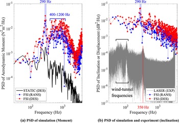
) in terms of the aerodynamic moment frequency spectrum. It appears that, when the wing is free to oscillate, the energy content at a frequency of 290 Hz is significantly enhanced, along with an increase in broadband noise between 400 and 1200 Hz. Additionally, figure 16(b) shows a comparison of the PSD between the simulation (inclination evolution) and the experiment (measured vertical displacement along the span). Both RANS and DES FSI simulations agree on the presence of a dominant oscillation frequency at 290 Hz. A similar peak at 350 Hz is also visible in the experimental data. This raises the question of whether the peak corresponds to the same oscillation mode.
$\alpha = 14.7^\circ$
) in terms of the aerodynamic moment frequency spectrum. It appears that, when the wing is free to oscillate, the energy content at a frequency of 290 Hz is significantly enhanced, along with an increase in broadband noise between 400 and 1200 Hz. Additionally, figure 16(b) shows a comparison of the PSD between the simulation (inclination evolution) and the experiment (measured vertical displacement along the span). Both RANS and DES FSI simulations agree on the presence of a dominant oscillation frequency at 290 Hz. A similar peak at 350 Hz is also visible in the experimental data. This raises the question of whether the peak corresponds to the same oscillation mode.
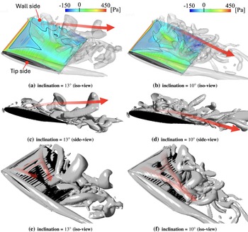
Details of the vortex structure and separation region. The colourmap refers to the shear stress distribution. The arrows indicate the main directions of the vortices.

Due to the heavy computational burden associated with FSI simulations, it is often not feasible to conduct a meaningful spectral orthogonal decomposition of the results to identify the driving mechanisms behind the main oscillation mode. However, it is still possible to analyse the variation in flow structures throughout an oscillation cycle, as shown in figure 17. Figures 17(a, c, e) and 17(b, d, f) refer to the vortex structures around the wing at the trough ( $\alpha = 13^\circ$
) and the peak (
$\alpha = 13^\circ$
) and the peak ( $\alpha = 10^\circ$
) of an oscillation period, respectively. The flow visualisation is performed using the swirling strength criterion, which corresponds to the imaginary part of the complex eigenvalues of
$\alpha = 10^\circ$
) of an oscillation period, respectively. The flow visualisation is performed using the swirling strength criterion, which corresponds to the imaginary part of the complex eigenvalues of $\nabla \mathbf{u}$
. The swirling strength threshold is set to 0.1.
$\nabla \mathbf{u}$
. The swirling strength threshold is set to 0.1.
Figure 17(a, b) also shows the surface shear-stress distribution to better visualise the extent of the separation region (i.e. areas of negative shear stress). Four main vortex structures can be identified: the tip vortex, the juncture vortex and two smaller vortices located on either side of the triangular separation region, which eventually merge into a larger vortex at midspan. The tip vortex promotes boundary-layer attachment and is typically aligned with the flow. The juncture vortex mainly influences the separation region near the wall. At the trough of the oscillation, the juncture vortex detaches from the wing and tends to follow the free-stream direction (as indicated by the red arrow). Conversely, at the peak of the oscillation ( $\alpha = 13^\circ$
), it moves closer to the wing surface and breaks down into smaller structures.
$\alpha = 13^\circ$
), it moves closer to the wing surface and breaks down into smaller structures.
Two vortices originate at the lateral edges of the midspan separation bubble. As shown in figure 17(e, f), these vortices tend to merge into a single, larger vortex – particularly evident at $\alpha = 13^\circ$
. It is known that two counter-rotating vortices become increasingly unstable as the free-stream velocity rises. Recent numerical simulations have detailed the mechanism behind the formation of bridges between such vortices. Based on these findings, it can be hypothesised that in the midspan region, two initially parallel vortices develop in the spanwise direction and eventually interact, giving rise to the two longitudinal vortices indicated by the arrows in figure 17(e, f). The bridges connecting these vortices are likely remnants of the original spanwise vortex structures. This dynamic is well described by the work of Yao & Hussain (Reference Yao and Hussain2022).
$\alpha = 13^\circ$
. It is known that two counter-rotating vortices become increasingly unstable as the free-stream velocity rises. Recent numerical simulations have detailed the mechanism behind the formation of bridges between such vortices. Based on these findings, it can be hypothesised that in the midspan region, two initially parallel vortices develop in the spanwise direction and eventually interact, giving rise to the two longitudinal vortices indicated by the arrows in figure 17(e, f). The bridges connecting these vortices are likely remnants of the original spanwise vortex structures. This dynamic is well described by the work of Yao & Hussain (Reference Yao and Hussain2022).
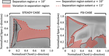
Variation in separation region extent according to steady and FSI simulations.

Pitching moment distribution on the wing at stall conditions: (a, b) mean and standard deviation; (c–j) distribution through roughly a period of oscillation ( $T = \textit{1}/f_{JW}\!$
).
$T = \textit{1}/f_{JW}\!$
).

As mentioned, it is the juncture vortex that primarily affects the separation region. Additionally, this effect differs significantly from the steady-state predictions, as shown in figure 18. On the left-hand side, the maximum variation in the separation region between inclinations of $10^\circ$
and
$10^\circ$
and $13^\circ$
is shown according to steady-state RANS simulations. In this case, the separation region primarily grows in the spanwise direction. Conversely, as shown on the right-hand side of the figure, the separation region changes are much more contained in the FSI case. The
$13^\circ$
is shown according to steady-state RANS simulations. In this case, the separation region primarily grows in the spanwise direction. Conversely, as shown on the right-hand side of the figure, the separation region changes are much more contained in the FSI case. The $10^\circ$
case appears similar for both FSI and steady simulations. However, at larger angles of attack, the extent of the separation region does not vary significantly in the FSI case, contrary to steady-state predictions.
$10^\circ$
case appears similar for both FSI and steady simulations. However, at larger angles of attack, the extent of the separation region does not vary significantly in the FSI case, contrary to steady-state predictions.
Figures 19(a) and 19(b) show the mean and standard deviation of the non-dimensional moment distribution on the wing. The moment coefficient can be written as $c_m = \Delta c_p (x/c)$
, where
$c_m = \Delta c_p (x/c)$
, where $\Delta c_p$
is the pressure difference between the two sides of the wing normalised by the dynamic pressure
$\Delta c_p$
is the pressure difference between the two sides of the wing normalised by the dynamic pressure $q$
, and
$q$
, and $(x/c)$
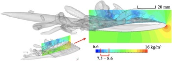
is the local non-dimensional distance from the pivot axis. Referring to figure 19(a), the leading edge is the part mainly contributing to the moment production; the moment values show two minima near the sidewall and near the tip, corresponding to juncture and tip vortex locations. A local increase in flow speed contributes to a reduction in static pressure, thus reducing the moment generated. Figure 19(b) shows that exactly where the mean moment distribution presents the minimum value, the variation is the largest. Particularly, the juncture vortex shedding is the main contributor to the variation in moment distribution. It is possible to dynamically observe this state of affairs through figure 19(c–j), where the instantaneous moment distribution is shown over a representative oscillation period. In terms of pressure variation, the juncture vortex results in a vortical structure forming near the sidewall at midchord and travelling downstream. There is now sufficient evidence to claim that the vibrations are caused by the juncture vortex, which affects the separation region near the sidewall. The next two sections are devoted to clarifying the effect of mesh refinement near the sidewall and providing a simple model to predict the oscillation frequency of the juncture vortex.
$(x/c)$
is the local non-dimensional distance from the pivot axis. Referring to figure 19(a), the leading edge is the part mainly contributing to the moment production; the moment values show two minima near the sidewall and near the tip, corresponding to juncture and tip vortex locations. A local increase in flow speed contributes to a reduction in static pressure, thus reducing the moment generated. Figure 19(b) shows that exactly where the mean moment distribution presents the minimum value, the variation is the largest. Particularly, the juncture vortex shedding is the main contributor to the variation in moment distribution. It is possible to dynamically observe this state of affairs through figure 19(c–j), where the instantaneous moment distribution is shown over a representative oscillation period. In terms of pressure variation, the juncture vortex results in a vortical structure forming near the sidewall at midchord and travelling downstream. There is now sufficient evidence to claim that the vibrations are caused by the juncture vortex, which affects the separation region near the sidewall. The next two sections are devoted to clarifying the effect of mesh refinement near the sidewall and providing a simple model to predict the oscillation frequency of the juncture vortex.
5. Effect of localised mesh refinements
The wing oscillates at around a stalled position. It is necessary at this point to understand if the vortex shedding is affected by the mesh refinement near the sidewall. The mesh used so far underwent a mesh independence study for an angle of attack of 6° (as shown in figure 6). However, it appears that the physics of the problem is considerably different near stall due to the dynamics of the juncture vortex. For the results shown so far, the original value of the first cell width near the wall was $\Delta z_w = 6$
mm, which appears too large considering the juncture vortex has a relative diameter of approximately 20–40 mm. The results of a new mesh independence study are shown in figure 20. Multiple simulations were conducted at stall conditions (
$\Delta z_w = 6$
mm, which appears too large considering the juncture vortex has a relative diameter of approximately 20–40 mm. The results of a new mesh independence study are shown in figure 20. Multiple simulations were conducted at stall conditions ( $\alpha = 14.7^\circ$
) for different values of refinement near the sidewall of the wing. Figure 20(a, b) shows the evolution of the net aerodynamic moment around the pivot; it is clear that with increasing levels of refinement, both the oscillation amplitude and mean value decrease with respect to the original values. In quantitative terms, figure 20(c) shows that the mean and standard deviation of the moment evolution change significantly, with the mean value moving from −0.7 to −1.8 N m and the amplitude of oscillation decreasing by approximately 50 %. In view of these results,
$\alpha = 14.7^\circ$
) for different values of refinement near the sidewall of the wing. Figure 20(a, b) shows the evolution of the net aerodynamic moment around the pivot; it is clear that with increasing levels of refinement, both the oscillation amplitude and mean value decrease with respect to the original values. In quantitative terms, figure 20(c) shows that the mean and standard deviation of the moment evolution change significantly, with the mean value moving from −0.7 to −1.8 N m and the amplitude of oscillation decreasing by approximately 50 %. In view of these results, $\Delta z_w = 0.0163$
mm is chosen for the following analysis. A frequency spectrum comparison between the original case and the refined mesh is shown in figure 20(d, e). While there is no clear significant difference between the two trends, the refined case shows an additional peak at about 420 Hz. The question arises of whether a new aeroelastic simulation will show results substantially different from those of the standard unrefined case.
$\Delta z_w = 0.0163$
mm is chosen for the following analysis. A frequency spectrum comparison between the original case and the refined mesh is shown in figure 20(d, e). While there is no clear significant difference between the two trends, the refined case shows an additional peak at about 420 Hz. The question arises of whether a new aeroelastic simulation will show results substantially different from those of the standard unrefined case.
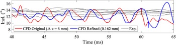
Figure 21 shows a comparison between original and refined mesh in terms of oscillation evolution. For the sake of simplicity and rapid comparison, the refined simulation was run for a few tenths of a millisecond and was initialised with the same data from the original mesh for a more accurate comparison. The two trends are very similar in terms of both frequency and amplitude. For the refined case, figure 22 shows a comparison between rigid and FSI cases in terms of standard deviation of the pressure distribution. It is possible to observe that, besides the very similar distributions, wing oscillations amplify the pressure variations by almost 40 %. Again, analogously to the original case (see figure 19 b), the majority of the moment variation is due to pressure fluctuations in the proximity of the sidewall towards the trailing edge of the plate, thus confirming that the main driving phenomena are captured even when using coarser meshes. From this analysis, it is possible to reinforce the hypothesis that oscillations are caused by juncture vortex shedding near the trailing edge.
Effect of additional refinement in the span direction near the sidewall in the proximity of the juncture vortex.

Comparison between original and refined cases in terms of aeroelastic response.

Standard deviation in pitching moment distribution on the wing for the rigid (immovable) and FSI cases for the refined case.

6. Juncture vortex frequency
The next challenge is to model this moving juncture vortex and its effect on the wing dynamics. It appears that the vibrations are one-way coupled: they are driven by the vortex dynamics and only weakly influenced by the wing motion. Under this assumption, the oscillation frequency can be approximated by the fundamental frequency of the vortex tube. From the visualisation of the flow field, the motion of the juncture vortex resembles that of a fluid-filled hosepipe. In this case, the governing equation for the vortex filament can be written as a wave equation:
 \begin{equation} \rho _{{eff}} A \frac {\partial ^2 \chi }{\partial t^2} = T \frac {\partial ^2 \chi }{\partial s^2}, \end{equation}
where the left-hand side represents the effective inertia of the vortex filament, with $\rho _{{eff}} A$
as the mass per unit length and
$\rho _{{eff}} A$
as the mass per unit length and $\chi (\mathbf{x},\,t)$
the filament position. The right-hand side is the restoring force due to the vortex tension
$\chi (\mathbf{x},\,t)$
the filament position. The right-hand side is the restoring force due to the vortex tension $T$
, and
$T$
, and $s$
is the coordinate along the vortex filament (which can be approximated by
$s$
is the coordinate along the vortex filament (which can be approximated by $x$
for moderate deflections). The vortex tension
$x$
for moderate deflections). The vortex tension $T$
can be approximated following Tsai & Widnall (Reference Tsai and Widnall1975) and Widnall et al. (Reference Widnall, Bliss and Tsai1974) as
$T$
can be approximated following Tsai & Widnall (Reference Tsai and Widnall1975) and Widnall et al. (Reference Widnall, Bliss and Tsai1974) as $T \sim \rho \varGamma ^2$
. The fundamental frequency can then be written as
$T \sim \rho \varGamma ^2$
. The fundamental frequency can then be written as
 \begin{equation} f_1 \sim \frac {1}{2l} \sqrt {\frac {\rho \varGamma ^2}{\rho _{{eff}} A}} \sim \frac {1}{2c} \sqrt {\frac {\varGamma ^2}{A}}, \end{equation}
where $l$
is approximated as the chord
$l$
is approximated as the chord $c$
and
$c$
and $\rho _{{eff}} \approx \rho$
. This latter approximation can be justified by examining figure 23, where density variations through the juncture vortex are expected to be smaller than 15 %. The frequency can then be expressed as
$\rho _{{eff}} \approx \rho$
. This latter approximation can be justified by examining figure 23, where density variations through the juncture vortex are expected to be smaller than 15 %. The frequency can then be expressed as
 \begin{equation} f_1 \sim \frac {\varGamma }{cd \sqrt {\pi }}. \end{equation}
From the simulations, the mean circulation of the juncture vortex is $\varGamma = 1.04 \pm 1.17$
m
$\varGamma = 1.04 \pm 1.17$
m $^2$
s−1 while the maximum vortex diameter is less than
$^2$
s−1 while the maximum vortex diameter is less than $0.4c$
, so we can estimate
$0.4c$
, so we can estimate $d = 0.2c$
to be an average core diameter. Based on these calculations, it is possible to isolate a frequency range of
$d = 0.2c$
to be an average core diameter. Based on these calculations, it is possible to isolate a frequency range of $f_1 \simeq 20$
–
$f_1 \simeq 20$
– $380$
Hz. The oscillation frequency peaks observed in simulations and experiments are 290 and 350 Hz, respectively. Based on this analysis, a simplified criterion for the juncture vortex frequency can be proposed:
$380$
Hz. The oscillation frequency peaks observed in simulations and experiments are 290 and 350 Hz, respectively. Based on this analysis, a simplified criterion for the juncture vortex frequency can be proposed:
 \begin{equation} f_{JW} \sim \frac {\varGamma }{cd}. \end{equation}
That is, the juncture vortex frequency is approximately equal to the mean vortex circulation divided by the product of the chord and the mean vortex diameter. For this configuration presented herein, the so calculated frequency is $f_{JW}\sim 310$
Hz.
$f_{JW}\sim 310$
Hz.
Density distribution around the juncture vortex.

7. Conclusion
In this work, the dynamics of a short, symmetric wing free to oscillate around a pivot point was studied numerically and experimentally in a transonic wind tunnel. The free-stream Mach number was 0.77, which exceeds the critical Mach number for small angles of attack. The pivot was located near the quarter-chord position. Due to aerodynamic instability about the pivot, the wing reached equilibrium only at large inclination angles of approximately $\pm 14^\circ$
, corresponding to deep-stall conditions. Simulation results were compared with experiments in terms of oscillation frequency and amplitude. In each experimental campaign, the wing oscillated around a slightly different equilibrium point near
$\pm 14^\circ$
, corresponding to deep-stall conditions. Simulation results were compared with experiments in terms of oscillation frequency and amplitude. In each experimental campaign, the wing oscillated around a slightly different equilibrium point near $\pm 13.5^\circ$
with an amplitude of approximately 1
$\pm 13.5^\circ$
with an amplitude of approximately 1 $^\circ$
. Conversely, in the simulation the oscillation amplitude was as large as 5
$^\circ$
. Conversely, in the simulation the oscillation amplitude was as large as 5 $^\circ$
. The calculated dominant oscillation frequency is approximately 290 Hz, thus close to the measured value of 350 Hz. The following conclusions can be drawn:
$^\circ$
. The calculated dominant oscillation frequency is approximately 290 Hz, thus close to the measured value of 350 Hz. The following conclusions can be drawn:
-
(i) Steady-state RANS simulations with rigid/not-moving geometry can accurately predict the location of the equilibrium point, even in the presence of large separated regions characteristic of deep stall. However, oscillation frequencies estimated from the local aerodynamic moment slope at the equilibrium point are unreliable.
-
(ii) Transient DES with rigid/not-moving geometry can predict the dominant oscillation frequency induced by juncture vortices. The frequency peak closely matches that observed in FSI simulations, indicating that wing motion has limited influence on the vortex shedding dynamics under deep-stall conditions.
-
(iii) FSI simulations identified the primary driving mechanism of the oscillations as a juncture vortex near the sidewall, oscillating mainly in the vertical direction. Away from the wall, the vortex retains a helical structure, but when collapsing onto the wing, it breaks down into smaller vortical structures. The separation pattern differs significantly from that predicted by steady simulations, with the flow remaining relatively attached except near the midspan region and close to the wall.
-
(iv) FSI simulations using both DES and RANS turbulence models yield comparable results in terms of oscillation amplitude and frequency, indicating that the choice between the two has a limited impact in this specific configuration.
Finally, to estimate the oscillation frequency induced by the juncture vortex, a simplified criterion was proposed, in which the frequency is approximated as the mean circulation along the vortex divided by the product of the chord and the average vortex diameter. Further experimental investigations are required to validate the accuracy and applicability of this criterion.
Supplementary movie
Supplementary movie is available at https://doi.org/10.1017/flo.2026.10056.
Acknowledgements
This work was funded by National Science and Technology Council (NSTC) under grant NSTC 113-2221-E-006-187. Computational and storage resources were kindly provided by the National Center for High-Performance Computing (NCHC). Special thanks go to the Head of Aerospace Science and Technology Research Center (ASTRC), Director C. Kung-Ming for supporting this research project.
Declaration of interests
The authors report no conflict of interest.


 6∘
6∘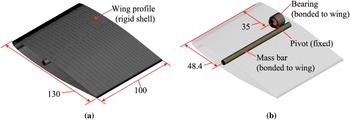
 ∂CM/∂α
 ∂CL/∂α
 xCP
xCP


 ±0.5∘
±0.5∘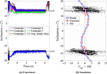


 T=1/fJW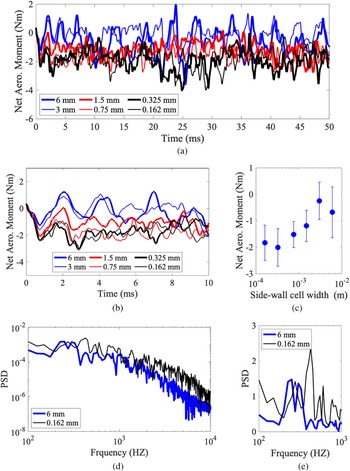



 Open access

