


Nomenclature
- ${a_t}$
-
action space
- DOF
-
degree of freedom
- DDPG
-
deep deterministic policy gradient
- DS
-
dynamic soaring
-
${F_x}$
-
force in x-axis of body frame
-
${F_y}$
-
force in y-axis of body frame
-
${F_z}$
-
force in z-axis of body frame
- g
-
gravitational acceleration
- GAE
-
generalised advantage estimation
-
${I_{xx}}$
-
moment of inertia about x-axis
-
${I_{yy}}$
-
moment of inertia about y-axis
-
${I_{zz}}$
-
moment of inertia about z-axis
- KE
-
kinetic energy
- KL
-
Kullback–Leibler divergence
- l
-
nominal wingspan
- m
-
nominal mass
-
${M_x}$
-
moment in x-axis of body frame
-
${M_y}$
-
moment in y-axis of body frame
-
${M_z}$
-
moment in z-axis of body frame
- N
-
experience buffer size
- OU
-
Ornstein-Uhlenbeck (OU) noise
- p
-
rotation about the body x-axis
- PE
-
potential energy
- PPO
-
proximal policy optimisation
- q
-
rotation about the body y-axis
- Q
-
dynamic pressure
- Q’
-
target network
- r
-
rotation about the body z-axis
-
${r_t}$
-
reward function
- ReLU
-
rectified linear unit
- RL
-
reinforcement learning
-
${s_t}$
-
state space
- t
-
time
- TD
-
temporal difference error
- TE
-
total energy
-
${T_i}$
-
thrust of i-th rotor
- TRPO
-
trust region policy optimisation
- u
-
velocity along the body x-axis
- UAV
-
unmanned aerial vehicle
- v
-
velocity along the body y-axis
-
${V_a}$
-
aircraft speed
-
${V_\phi }$
s(t)
-
value function
-
${V_{ref}}$
-
wind speed at reference altitude
-
${V_z}$
-
wind speed
- w
-
velocity along the body z-axis
- x
-
position in x-direction
- y
-
position in y-direction
- z
-
position in z-direction
-
${z_0}$
-
surface correction factor
-
${z_{ref}}$
-
reference altitude


Greek symbol
-
$\alpha $
-
angle-of-attack
-
$\beta $
-
sideslip angle
-
$\gamma $
-
flight path angle
-
$\gamma {^{\prime}}$
-
discount factor
-
$\delta $
-
KL-divergence limit
-
${\phi _B}$
-
bank angle
-
$\theta $
-
pitch angle
-
$\psi $
-
heading angle
-
$\rho $
-
air density
-
$\mu $
-
target policy
-
$\mu {^{\prime}}$
-
target network
-
${\pi _\theta }$
-
current policy
-
$\sigma $
-
tilt angle of rotor
-
$\tau $
-
target update rate


1.0 Introduction
Dynamic soaring (DS) is a flight technique that enables aerial vehicles to harvest energy from wind shear, thereby sustaining flight without continuous propulsion. This phenomenon has been extensively studied in biological systems, particularly in seabirds such as the albatross, which can traverse long distances over the ocean with minimal flapping [Reference Rayleigh1, Reference Sachs2]. Recent studies have extended this concept to unmanned aerial vehicles (UAVs), demonstrating that properly optimised DS trajectories can significantly enhance endurance and range [Reference Bousquet, Triantafyllou and Slotine3].
The seminal work on DS was done by Lord Rayleigh in 1883 by understanding the basis of such flight demonstrated by soaring birds [Reference Boslough4–Reference Wood6]. Realising its importance during flight, various studies have been directed to understand and identify the aspects of DS by utilising various optimisation techniques. Initially, the study of this phenomena was limited to fixed platform configurations, where the model has a fixed geometry during its flight [Reference Bonnin, Bénard, Moschetta and Toomer7–Reference Deittert, Richards, Toomer and Pipe10]. However, the soaring birds have been observed to continuously change the shape and size of their wings while exhibiting DS during flight [Reference Pennycuick11]. DS manoeuvre was investigated for a morphing platform [Reference Mir, Maqsood and Akhtar12]. DS requires wind shear; that is, the wind profile varies with the altitude for the effective execution of this manoeuvre. As a result, this phenomenon is utilised by propeller- and jet-driven small UAVs either for an un-powered flight or flight with minimum fuel utilisation [Reference Zhao and Celia Qi13].
Conventional approaches for DS trajectory generation often rely on optimal control methods or energy-based models [Reference Lawrance and Sukkarieh14]. However, such methods are limited by model accuracy and computational cost, especially in highly dynamic environments. In contrast, reinforcement learning (RL) has recently emerged as a powerful tool for autonomous decision-making in UAVs, providing adaptability to complex aerodynamic interactions [Reference Lillicrap, Hunt, Pritzel, Heess, Erez, Tassa, Silver and Wierstra15–Reference Wakefield, Phillips, Matthiopoulos, Fukuda, Higuchi, Marshall and Trathan22]. Prior studies show that DS paths generally fall into two categories: closed-loop trajectories, where the vehicle returns to its starting position (e.g. the circular/loitering patterns studied by Sachs [Reference Sachs and Grüter23] and Wang [Reference Wang, An and Song24]), and open-loop trajectories, where the vehicle continues progressing forward without returning to the initial coordinates [Reference Wang, An and Song21, Reference Sachs and Grüter25, Reference Zwenig, Hong and Holzapfel26]. These investigations identify two primary soaring modes: (i) loiter mode, characterised by a circular, banked, energy-harvesting loop with fully constrained start-and-end positions, and (ii) forward or basic mode, which permits net horizontal progression along the wind direction. Since typical UAV missions require forward travel over a defined distance, this work adopts the open-loop dynamic-soaring mode, which allows unconstrained horizontal progression and better aligns with practical UAV mission requirements. Refer to Fig. 1 for a 3D graphical depiction of the respective DS manoeuvre, which typically consists of four phases: windward climb, high altitude turn, leeward descent and low altitude turn [Reference Mir, Eisa and Maqsood27].
The conceptual open-loop DS trajectory. Blue colour shows the 3D trajectory, dashed lines are the trajectory projections in three directions.

To perform DS, soaring birds exploit the wind shear, which is a physical phenomenon characterised by a significant change in wind speed with altitude, commonly found over oceans and seas [Reference Bousquet, Triantafyllou and Slotine3, Reference Mir, Eisa and Maqsood27, Reference Mir, Eisa, Taha, Maqsood, Akhtar and Ul Islam28]. The birds initiate the manoeuvre by flying into the headwind, gaining lift as they ascend through this shear layer. This upward motion continues until they reach a point where further altitude gain is no longer possible. At that stage, they execute a high-altitude turn and begin a descent, effectively converting potential energy into kinetic energy. Upon reaching the lowest viable altitude, a low-altitude turn is performed, initiating a new DS cycle. Through this mechanism, birds manage to cover distance with minimal or no energy expenditure. The DS behaviour observed in birds has been experimentally validated in biological studies [Reference Sachs, Traugott, Nesterova and Bonadonna29, Reference Yonehara, Goto, Yoda, Watanuki, Young, Weimerskirch, Bost and Sato30]. For unmanned aircraft, carefully timed climbs into headwind and dives with tailwind, connected by crosswind turns, can sustain airspeed while keeping total energy approximately constant. Numerical optimisation approaches [Reference Betts31] have been widely applied to DS, framing it as a trajectory optimisation problem in which the objective is to identify a path that enables an energy-neutral (or near-neutral) DS cycle.
DS manoeuvre generally involves roll, pitch and yaw movements. A heuristic approach for deriving aerodynamic variables of a UAV was given by Wharington [Reference Wharington32] to formulate DS trajectories. With the help of these heuristics, a closed-loop controller was designed to control an aircraft to perform DS autonomously. But this study could not conclude to a function that would predict speed gain at each loop of manoeuvre [Reference Ariff and Go33], hence this heuristic control approach was marked ineffective [Reference Bye and McClure34]. It was concluded that open-loop heuristics are best described by a sinusoidal airspeed function with a vertical wind gradient. Based on this, Ariff and Go [Reference Ariff and Go35] worked to formulate a trajectory-generating algorithm using the concept of Dubins curves in terms of differential geometry. Simulations of these showed that this technique reduces the computation time by half or more without affecting the results.
The integration of RL algorithms in the control of UAVs, especially during complex manoeuvres, has garnered significant attention in recent research. The work of Akhtar et al. [Reference Akhtar and Maqsood36] emphasises the use of RL for optimising hover-to-cruise transitions in tilt-rotor UAVs. They found that proximal policy optimisation (PPO) provided superior stability and convergence compared to deep deterministic policy gradient (DDPG) and trust region policy optimisation (TRPO), showcasing the effectiveness of RL in complex manoeuvring scenarios. Similarly, a few other studies [Reference Akhtar, Maqsood and Verbeke37, Reference Akhtar and Maqsood38] focus on using DDPG particularly for optimising complex UAV trajectories. Montella et al. [Reference Montella and Spletzer39] highlighted the potential of RL in DS by demonstrating that it can outperform traditional controllers by adapting trajectories in real-time, thus enhancing energy efficiency.
Early applications of RL to soaring were demonstrated by Wharington et al. [Reference Wharington40] in simulation and by Reddy et al. [Reference Reddy, Celani, Sejnowski and Vergassola41, Reference Reddy, Jerome Wong-Ng, Sejnowski and Vergassola42] on a real glider, using a rule-based state-action-reward-state-action (SARSA) agent in wind-free environments. The control policy was implemented as a lookup table mapping discretised states to discretised bank-angle actions. Its limited representational capacity suggests that richer learning architectures can yield improved performance. Cui et al. [Reference Cui, Yan and Wan43] implemented a soaring strategy, known as SAC (soft actor-critic), that considers continuous processes. SAC employs a stochastic maximum-entropy policy to enhance exploration, but its performance is sensitive to entropy tuning. Moreover, it outputs a probability distribution over actions rather than a single deterministic decision, from which actions are sampled [Reference Haarnoja, Zhou, Abbeel and Levine44]. In contrast, DDPG, PPO and TRPO provide stable learning and robust policy updates through deterministic or trust-region–based optimisation [Reference Lillicrap, Hunt, Pritzel, Heess, Erez, Tassa, Silver and Wierstra15, Reference Schulman, Wolski, Dhariwal, Radford and Klimov16], making them well suited for the DS scenarios considered in this work.
In addition to RL and optimal control methods, recent work has explored extremum seeking control (ESC) as a model-free, real-time optimisation strategy for DS. ESC methods iteratively perturb control inputs and use real-time measurements to steer the system toward an optimum without requiring an explicit model of the dynamics or wind profiles. This contrasts with traditional optimal control frameworks and RL approaches that depend on computationally expensive offline training or precise models. Recent studies [Reference Pokhrel and Eisa45, Reference Eisa and Pokhrel46] have shown that ESC can autonomously and robustly achieve energy-efficient soaring behaviour, and may better capture the biological mechanisms used by birds like albatrosses to soar in uncertain wind environments.
The goal of this study is to develop an optimal control strategy for a tricopter hybrid UAV to perform DS manoeuvre by autonomously exploiting environmental wind shear. DS involves extracting energy from horizontal or vertical wind gradients, enabling the UAV to sustain or gain altitude without continuous thrust input. This is particularly valuable in scenarios where onboard energy is limited and external aerodynamic energy must be harnessed for extending flight endurance.
The objective is to generate an energy-optimal trajectory that allows the UAV to ascend and descend through regions of varying wind velocity, mimicking the energy-harvesting behaviour observed in birds such as albatrosses. This requires the UAV to learn how to modulate its control inputs such as thrust distribution, bank angle and attitude to gain energy from the wind while maintaining flight stability and adhering to system constraints.
1.1 Gaps and contributions
Although significant progress has been made in DS and learning-based UAV control, several key gaps remain, particularly for hybrid tricopter UAVs. Most prior studies focus on fixed-wing or conventional multicopter platforms, leaving the feasibility and stability of DS in tricopter tilt-rotor configurations largely unexplored. Additionally, there is limited understanding of how different RL algorithms perform under identical environmental conditions and UAV initial states, especially in terms of energy management, trajectory regularity and control smoothness.
These gaps hinder the development of robust, energy-efficient and adaptive controllers for thrust-preserving manoeuvres in hybrid UAVs. In particular, DS has been mostly analysed for fixed-wing or conventional multicopters, leaving the tricopter tilt-rotor configuration largely unstudied. Furthermore, the feasibility of executing stable, near-constant total energy DS cycles in hybrid tricopters remains unclear. Existing research also lacks a comparative analysis of different RL algorithms under identical initial states and wind profiles for DS. In addition, many studies overlook realistic wind effects and the role of intermittent forward-thrust ‘top-ups’ during DS cycles. Finally, there is limited evidence on how controllers maintain smooth three-dimensional trajectories while preserving energy neutrality, leaving trajectory regularity and control smoothness largely unexplored.
To address the limitations identified above, this work presents several key contributions aimed at advancing autonomous control, energy-efficient manoeuvres and the application of deep RL for unconventional hybrid UAVs. First, a control-affine DS environment is formulated for a hybrid UAV, capturing gliding phases, sparse forward-thrust ‘top-ups’ and shear-layer wind effects during the DS cycle. Second, three RL algorithms – DDPG, TRPO and PPO – are implemented on the UAV to enable effective learning of the DS task. Third, a comparative evaluation of these algorithms is conducted, analysing energy neutrality ( ${{\Delta }}$
TE over a cycle), trajectory regularity in three-dimensional space and control smoothness under identical initial states and wind fields. Finally, empirical results demonstrate that the UAV can achieve near-constant total energy over a DS cycle with the characteristic exchange between kinetic and potential energy, while highlighting how PPO, TRPO and DDPG differ in their ability to maintain energy neutrality and produce smooth trajectories.
${{\Delta }}$
TE over a cycle), trajectory regularity in three-dimensional space and control smoothness under identical initial states and wind fields. Finally, empirical results demonstrate that the UAV can achieve near-constant total energy over a DS cycle with the characteristic exchange between kinetic and potential energy, while highlighting how PPO, TRPO and DDPG differ in their ability to maintain energy neutrality and produce smooth trajectories.
To our knowledge, this is the first study to systematically evaluate PPO, TRPO and DDPG for DS on such a UAV. These algorithms are selected because DS requires stable learning in continuous, nonlinear and stochastic environments, a regime where trust-region and actor–critic methods consistently outperform discrete or model-dependent approaches.
2.0 UAV and flight dynamics modeling
The UAV’s dynamics are modeled using a 6-degree-of-freedom (6-DOF) nonlinear flight model, capturing translational and rotational motions under aerodynamic forces and rotor thrust from the front two rotors only. Due to the complex, coupled nature of these dynamics and the stochastic wind profile, traditional optimisation approaches become not tractable. Mathematically, the problem can be framed as a continuous-time, continuous-action optimisation task. Therefore, we formulate this problem using an RL framework, where the UAV (agent) must learn a sequence of control actions ${a_t}$
given a state
${a_t}$
given a state ${s_t}$
, such that the cumulative reward
${s_t}$
, such that the cumulative reward ${r_t}$
is maximised. The reward is designed to favour energy gain, efficient manoeuvring and adherence to flight boundaries. The agent learns an optimal policy
${r_t}$
is maximised. The reward is designed to favour energy gain, efficient manoeuvring and adherence to flight boundaries. The agent learns an optimal policy $\pi $
that maps states to actions through trial-and-error interaction with the environment. This policy is subject to the UAV flight dynamics,vwind profile modeled as a continuous shear function (logarithmic model) and constraints on altitude, velocity and rotor thrust.
$\pi $
that maps states to actions through trial-and-error interaction with the environment. This policy is subject to the UAV flight dynamics,vwind profile modeled as a continuous shear function (logarithmic model) and constraints on altitude, velocity and rotor thrust.
2.1 UAV model
This work considers a hybrid tricopter UAV whose front two propellers are fixed, forward-facing and provide thrust only when required, while the tail rotor remains idle during the manoeuvre (Fig. 2). This configuration simplifies the mechanism relative to tilt-prop systems and emphasises the gliding dynamics of DS. It also tightens control authority: longitudinal thrust must be scheduled sparingly to preserve energy neutrality; attitude and path shaping must come primarily from aerodynamic loading and crosswind manoeuvring. The UAV under consideration has a wing span ‘l’ of 0.61 m and a mass ‘m’ of 1.5 kg. The rotors are labeled as ${R_1}$
,
${R_1}$
, ${R_2}$
and
${R_2}$
and ${R_3}$
where
${R_3}$
where ${\sigma _1}$
and
${\sigma _1}$
and ${\sigma _2}$
are the tilt angles for front rotors
${\sigma _2}$
are the tilt angles for front rotors ${R_1}$
and
${R_1}$
and ${R_2}$
, respectively. For simplicity, the rear rotor is assumed to remain inactive, while the front two rotors are modeled as fixed, non-tiltable propellers. The modeling parameters of the UAV are elaborated in Table 1.
${R_2}$
, respectively. For simplicity, the rear rotor is assumed to remain inactive, while the front two rotors are modeled as fixed, non-tiltable propellers. The modeling parameters of the UAV are elaborated in Table 1.
Schematic diagram of UAV considered: coordinate system and forces.

Modeling parameters of tricopter

2.2 Coordinate system
The coordinate system is illustrated in Fig. 2. The body-fixed axes are defined as follows: ${X_B}$
axis points forward from the tricopter’s perspective,
${X_B}$
axis points forward from the tricopter’s perspective, ${Y_B}$
axis extends to the right and
${Y_B}$
axis extends to the right and ${Z_B}$
axis points downward from the tricopter’s centre of gravity. The relationship between the inertial (earth-fixed) frame and the body frame can be described using the rotation matrix R
${Z_B}$
axis points downward from the tricopter’s centre of gravity. The relationship between the inertial (earth-fixed) frame and the body frame can be described using the rotation matrix R $\left({\phi ,\theta ,\psi } \right)$
. It is the direction cosine matrix (DCM) or coordinate transformation matrix. The vehicle’s orientation is represented by the Euler angles: roll (
$\left({\phi ,\theta ,\psi } \right)$
. It is the direction cosine matrix (DCM) or coordinate transformation matrix. The vehicle’s orientation is represented by the Euler angles: roll ( $\phi $
), pitch (
$\phi $
), pitch ( $\theta $
) and yaw (
$\theta $
) and yaw ( $\psi $
), which correspond to rotations about
$\psi $
), which correspond to rotations about ${X_B}$
,
${X_B}$
, ${Y_B}$
and
${Y_B}$
and ${Z_B}$
axes, respectively. The transformation from the inertial (navigation) frame (X,Y,Z) to the body frame (
${Z_B}$
axes, respectively. The transformation from the inertial (navigation) frame (X,Y,Z) to the body frame ( ${X_b},{Y_b},{Z_b}$
) is expressed through the DCM, as shown in Equation (1).
${X_b},{Y_b},{Z_b}$
) is expressed through the DCM, as shown in Equation (1).
 \begin{align}\left[ {\begin{array}{*{20}{c}}{{X_B}}\\{{Y_B}}\\{{Z_B}}\end{array}} \right] = R\left({\phi ,\theta ,\psi } \right)\left[ {\begin{array}{*{20}{c}}X\\Y\\Z\end{array}} \right]\end{align}
The rotation is first applied to the ${Z_B}$
axis with an angle of
${Z_B}$
axis with an angle of $\psi $
, then to the
$\psi $
, then to the ${Y_B}$
axis with an angle of
${Y_B}$
axis with an angle of $\theta $
, and finally the
$\theta $
, and finally the ${X_B}$
axis is rotated with an angle of
${X_B}$
axis is rotated with an angle of $\phi $
. The rotation matrix
$\phi $
. The rotation matrix $R\left({z,\psi } \right)$
along the z-axis, where
$R\left({z,\psi } \right)$
along the z-axis, where $\psi $
is the rolling angle along the z-axis, is given as Equation (2):
$\psi $
is the rolling angle along the z-axis, is given as Equation (2):
 \begin{align}R\left({z,\psi } \right) = \left[ {\begin{array}{*{20}{c}}{\cos\psi }&\quad{\sin\psi }&\quad0\\{ - \sin\psi }&\quad{\cos\psi }&\quad0\\0&\quad0&\quad 1\end{array}} \right]\end{align}
The rolling matrix $R\left({y,\theta } \right)$
, where
$R\left({y,\theta } \right)$
, where $\theta $
is the rotation angle along the y-axis, is as follows in Equation (3):
$\theta $
is the rotation angle along the y-axis, is as follows in Equation (3):
 \begin{align}R\left({y,\theta } \right) = \left[ {\begin{array}{*{20}{c}}{\cos\theta }&\quad 0&\quad { - \sin\theta }\\0&\quad 1&\quad 0\\{\sin\theta }&\quad 0&\quad {\cos\theta }\end{array}} \right]\end{align}
The rotation matrix $R\left({x,\phi } \right)$
rotates around the x-axis with a rotation angle
$R\left({x,\phi } \right)$
rotates around the x-axis with a rotation angle $\phi $
given as Equation (4):
$\phi $
given as Equation (4):
 \begin{align}R\left({x,\phi } \right) = \left[ {\begin{array}{*{20}{c}}1&\quad 0&\quad 0\\0&\quad {\cos\phi }&\quad {\sin\phi }\\0&\quad { - \sin\phi }&\quad {\cos\phi }\end{array}} \right]\end{align}
By combining the defined rotation matrices, the complete transformation from the inertial frame to the body frame can be obtained:
 \begin{align}R\left({\phi ,\theta ,\psi } \right) = R\left({z,\psi } \right)R\left({y,\theta } \right)R\left({x,\phi } \right)\end{align}
 \begin{align}DCM = \left({\phi ,\theta ,\psi } \right) = \left[\! {\begin{array}{*{20}{c}}{\cos\theta \cos\psi }&\quad {\cos\theta \sin\psi }&\quad { - \sin\theta }\\{\sin\phi \sin\theta \cos\psi - \cos\phi \sin\psi }&\quad {\sin\phi \sin\theta \sin\psi + \cos\phi \cos\psi }&\quad {\sin\phi \cos\theta }\\{\cos\phi \sin\theta \cos\psi + \sin\phi \sin\psi }&\quad {\cos\phi \sin\theta \sin\psi - \sin\phi \cos\psi }&\quad {\cos\phi \cos\theta }\end{array}} \!\right]\end{align}
2.3 Flight dynamics model
The tricopter UAV’s flight dynamics are governed by a six-degree-of-freedom (6-DOF) nonlinear model, which captures the translational and rotational motion of the vehicle in three-dimensional space. These dynamics are expressed in the body-fixed frame, with respect to the centre of gravity of the UAV, and are influenced by aerodynamic forces, propulsive forces (when active) and gravity.
The flight mechanics model of the drone in this article differs from that of conventional drones due to the usage of rotors along with a fixed wing. The rotor at aft is considered to be inactive, thus there is no thrust component in the force acting on the drone and no momentum change caused by the engine rotor in the torque calculation formula. However, the front two rotors provide a limited thrust according to mission requirement.
The model is described in terms of two aspects:
-
1. the translational dynamics (motion along body axes-
${X_B}$
,
${Y_B}$
,
${Z_B}$
) -
2. the rotational dynamics (angular motion about body axes-
$\phi $
,
$\theta $
,
$\psi $
)


The state of the UAV is described by its linear velocities u,v,w, angular rates p,q,r, Euler angles $\phi $
,
$\phi $
, $\theta $
,
$\theta $
, $\psi $
and inertial positions x,y,z. The translational dynamics of the UAV are governed by Newton’s Second Law, which relates the sum of external forces acting on the vehicle to the rate of change of its linear momentum.
$\psi $
and inertial positions x,y,z. The translational dynamics of the UAV are governed by Newton’s Second Law, which relates the sum of external forces acting on the vehicle to the rate of change of its linear momentum.
 \begin{align}&{\dot u} = v - qw + \dfrac{{{F_x}}}{m} - g\, {\sin} \, \theta \nonumber\\&{\dot v} = pw - ru + \dfrac{{{F_y}}}{m} - g \, {\cos} \, \theta \, {\sin}\, \phi \nonumber\\&{\dot w} = qu - pv + \dfrac{{{F_z}}}{m} - g \, {\cos} \, \theta\, {\cos} \, \phi \end{align}
where $m$
is mass of the UAV,
$m$
is mass of the UAV, $g$
is gravitational acceleration and
$g$
is gravitational acceleration and ${F_x},{F_y},{F_z}$
are the total forces in body frame, including aerodynamic (
${F_x},{F_y},{F_z}$
are the total forces in body frame, including aerodynamic ( ${F_a}$
), propulsive (
${F_a}$
), propulsive ( ${F_p}$
) and gravitational forces (
${F_p}$
) and gravitational forces ( ${F_g}$
) in each axis.
${F_g}$
) in each axis.
The rotational dynamics of the UAV are described by Euler’s equations, which relate the applied moments to the rates of change of the vehicle’s angular motion about its principal axes.
 \begin{align}&\dot{p} = \dfrac{{{I_{yy}} - {I_{zz}}}}{{{I_{xx}}}}qr + \dfrac{{{M_x}}}{{{I_{xx}}}} \nonumber\\&{\dot q} = \dfrac{{{I_{zz}} - {I_{xx}}}}{{{I_{yy}}}}pr + \dfrac{{{M_y}}}{{{I_{yy}}}} \nonumber\\&{\dot r} = \dfrac{{{I_{xx}} - {I_{yy}}}}{{{I_{zz}}}}pq + \dfrac{{{M_z}}}{{{I_{zz}}}}\end{align}
where ${I_{xx}},{I_{y{\textrm{y}}}},{I_{zz}}$
are the moments of inertia about the three axes in the body. For symmetric UAVs, the moments of inertia about the three planes (
${I_{xx}},{I_{y{\textrm{y}}}},{I_{zz}}$
are the moments of inertia about the three axes in the body. For symmetric UAVs, the moments of inertia about the three planes ( ${I_{xy}},{I_{yz}},{I_{zx}}$
are zero.
${I_{xy}},{I_{yz}},{I_{zx}}$
are zero. ${M_x},{M_y},{M_z}$
are the total moments in body frame. They include aerodynamic and propulsive moments.
${M_x},{M_y},{M_z}$
are the total moments in body frame. They include aerodynamic and propulsive moments.
The kinematics are described by the Euler angle rate equations.
 \begin{align}&{\dot \phi }{ = p + {\tan\,}\theta \left({q \, {\sin} \, \phi + r\, {\cos} \, \phi } \right)}\nonumber\\&{\dot \theta }{ = q\,{\cos} \, \,\phi - r\,{\sin}\,\phi }\nonumber\\&{\dot \psi }{ = \dfrac{{q\,{\sin} \,\phi + r\,{\cos} \, \,\phi }}{{{\cos} \, \,\theta }}}\end{align}
The dynamic pressure ( $Q$
) is a function of aircraft speed (
$Q$
) is a function of aircraft speed ( ${V_a}$
) and air density (
${V_a}$
) and air density ( $\rho $
):
$\rho $
):
 \begin{align}Q = \dfrac{1}{2}{{\rho }}V_a^2\end{align}
where the velocity ( ${V_a}$
) is given by the following equation:
${V_a}$
) is given by the following equation:
 \begin{align}{V_a} = \sqrt {{u^2} + {v^2} + {w^2}} \end{align}
The aerodynamic forces and gravitational forces in each of the three axis are given in Equation (13). Propulsive forces are those generated directly by the UAV’s rotors, and they act on its body.
These forces generated by all rotors are summed and expressed in the body frame of the UAV. The following considerations are made for the analysis: the rear rotor remains inactive throughout the flight, while the two front rotors are fixed in a forward-facing configuration without any tilt mechanism. Each rotor generates a thrust force ${T_i}$
(i = 1, 2) in the direction of its local axis and possibly a torque
${T_i}$
(i = 1, 2) in the direction of its local axis and possibly a torque ${\tau _i}$
depending on the rotation direction. Propulsion is utilised only during the ascent and descent phases, whereas the main flight phase consists of passive DS, during which the UAV harnesses wind energy for sustained flight.
${\tau _i}$
depending on the rotation direction. Propulsion is utilised only during the ascent and descent phases, whereas the main flight phase consists of passive DS, during which the UAV harnesses wind energy for sustained flight.
The propulsive forces generated by the rotors in the body frame are given by:
 \begin{align}\left[ {\begin{array}{*{20}{c}}{{X_p}}\\{{Y_p}}\\{{Z_p}}\end{array}} \right] = \mathop \sum \limits_{i = 1}^2 {T_i}\left[ {\begin{array}{*{20}{c}}{{\sin}\! \left({{\sigma _i}} \right)}\\{{\sin}\! \left({{\sigma _i}} \right)}\\{ - {\cos}\! \left({{\sigma _i}} \right)}\end{array}} \right]\end{align}
where ${T_i}$
is the thrust produced by the
${T_i}$
is the thrust produced by the $i$
-th rotor and
$i$
-th rotor and ${\sigma _i}$
is the rotor’s tilt angle. The notations and assumptions for rotor thrust are defined below:
${\sigma _i}$
is the rotor’s tilt angle. The notations and assumptions for rotor thrust are defined below:
-
1.
${T_1}$
,
${T_2}$
: Thrust from front-left and front-right rotors, respectively -
2. no tilt assumption:
${\sigma _i} = {90^ \circ } \Rightarrow {\sin} \, \left({{\sigma _i}} \right) = 1,\cos\left({{\sigma _i}} \right) = 0$
-
3. total rotor thrust:
${T_{{\textrm{total}}}} = {T_1} + {T_2}$
where
${T_{{\textrm{total}}}}$
is thrust for
${X_p}$
only (Equation (13))


The total force vector is expressed as the resultant of all external forces acting on the UAV. It comprises aerodynamic forces, gravitational forces and propulsive forces and is given in Equation (13).
 \begin{align}\left[ {\begin{array}{*{20}{c}}{{F}}\\{{F_y}}\\{{F_z}}\end{array}} \right] &= \underbrace {Q{S_{{\textrm{ref}}}}\left[ {\begin{array}{*{20}{c}}{ - {C_{{D_\alpha }}}{\cos} \, \alpha + {C_{{L_\alpha }}}{\sin} \, \alpha + ({ - {C_{{D_\alpha }}}{\cos} \, \alpha + {C_{{L_\alpha }}}{\sin} \, \alpha } )\dfrac{c}{{2{V_a}}}q}\\{{C_Y} + {C_{{Y_\beta }}}\beta + \dfrac{b}{{2{V_a}}}p{C_{{Y_p}}} + \dfrac{b}{{2{V_a}}}r{C_{{Y_r}}}}\\{ - {C_{{D_\alpha }}}{\sin} \, \alpha - {C_{{L_\alpha }}}{\cos} \, \alpha + ({ - {C_{{D_\alpha }}}{\sin} \, \alpha - {C_{{L_\alpha }}}{\cos} \, \alpha } )\dfrac{c}{{2{V_a}}}q}\end{array}} \right]}_{{\textrm{Aerodynamic forces}}}\nonumber\\&\quad + \underbrace {mg\left[ {\begin{array}{*{20}{c}}{ - {\sin} \, \theta }\\{{\cos} \, \theta \, {\sin} \, \phi }\\{{\cos} \, \theta \, {\cos} \, \phi }\end{array}} \right]}_{{\textrm{Gravitational forces}}} + \underbrace {\left[ {\begin{array}{*{20}{c}}{{T_1} + {T_2}}\\0\\0\end{array}} \right]}_{{\textrm{Propulsive forces}}}\end{align}
The general formula for a moment (torque) caused by a force applied at some point offset from the axis is:
 \begin{align}{\bf{M}} = \mathop \sum \limits_{i = 1}^2 \left({{{\bf{r}}_i} \times {{\bf{F}}_i}} \right)\end{align}
The magnitude of this moment is:
 \begin{align}\left\| {\bf{M}} \right\| = \mathop \sum \limits_{i = 1}^2 \left({\left\| {{{\bf{r}}_i}} \right\| \cdot \left\| {{{\bf{F}}_i}} \right\| \cdot {\sin} \, \left({{\sigma _i}} \right)} \right)\end{align}
where $r = l$
is the position vector,
$r = l$
is the position vector, $F = T$
= thrust vector and
$F = T$
= thrust vector and $\sigma $
is the angle between moment arm and thrust. The rotors are located at
$\sigma $
is the angle between moment arm and thrust. The rotors are located at $ \pm l$
on the y-axis, i.e. the front left rotor is located at
$ \pm l$
on the y-axis, i.e. the front left rotor is located at ${{\bf{r}}_1} = {[x, + l,0]^T}$
and front right rotor is at
${{\bf{r}}_1} = {[x, + l,0]^T}$
and front right rotor is at ${{\bf{r}}_2} = {[x, - l,0]^T}$
.
${{\bf{r}}_2} = {[x, - l,0]^T}$
.
 \begin{align}\left[ {\begin{array}{*{20}{c}}{Lp}\\{{M_p}}\\{{N_p}}\end{array}} \right] = \left[ {\begin{array}{*{20}{c}}{l \, {\cos} \, \left({{\sigma _1}} \right)}&\quad { - l \, {\cos} \, \left({{\sigma _2}} \right)}\\0&\quad 0\\{l \, {\sin} \, \left({{\sigma _1}} \right)}&\quad { - l \, {\sin} \, \left({{\sigma _2}} \right)}\end{array}} \right]\left[ {\begin{array}{*{20}{c}}{{T_1}}\\{{T_2}}\end{array}} \right] + \left[ {\begin{array}{*{20}{c}}{{\sin} \, {\sigma _1}}&\quad {{\sin} \, {\sigma _2}}\\0&\quad 0\\{ - {\cos} \, {\sigma _1}}&\quad { - {\cos} \, {\sigma _2}}\end{array}} \right]\left[ {\begin{array}{*{20}{c}}{ - {M_1}}\\{{M_2}}\end{array}} \right]\end{align}
Since no tilt is considered for rotors, so ${\sigma _i} = {90^ \circ } \Rightarrow {\sin} \, \left({{\sigma _i}} \right) = 1,{{\cos}}\left({{\sigma _i}} \right) = 0$
 \begin{align}\left[ {\begin{array}{*{20}{c}}{Lp}\\{{M_p}}\\{{N_p}}\end{array}} \right] = \left[ {\begin{array}{*{20}{c}}0&\quad 0\\0&\quad 0\\l&\quad { - l}\end{array}} \right]\left[ {\begin{array}{*{20}{c}}{{T_1}}\\{{T_2}}\end{array}} \right] + \left[ {\begin{array}{*{20}{c}}1&\quad 1\\0&\quad 0\\0&\quad 0\end{array}} \right]\left[ {\begin{array}{*{20}{c}}{ - {M_1}}\\{{M_2}}\end{array}} \right]\end{align}
 \begin{align}\left[ {\begin{array}{*{20}{c}}{Lp}\\{{M_p}}\\{{N_p}}\end{array}} \right] = \left[ {\begin{array}{*{20}{c}}{ - {M_1} + {M_2}}\\0\\{l\left({{T_1} - {T_2}} \right)}\end{array}} \right]\end{align}
The total moments $\left({{M_x},{M_y},{M_z}} \right)$
are calculated from the aerodynamic moments and propulsive moments, which are given in Equation (19).
$\left({{M_x},{M_y},{M_z}} \right)$
are calculated from the aerodynamic moments and propulsive moments, which are given in Equation (19).
 \begin{align}\left[ {\begin{array}{*{20}{c}}{{M_x}}\\{{M_y}}\\{{M_z}}\end{array}} \right] = \underbrace {Q{S_{{\textrm{ref}}}}\left[ {\begin{array}{*{20}{c}}{\bar b\left({{C_L} + {C_{{L_\beta }}}\beta + {C_{{L_p}}}\dfrac{{\bar b}}{{2{V_a}}}p + {C_{{L_r}}}\dfrac{{\bar b}}{{2{V_a}}}r} \right)}\\{c\left({{C_M} + {C_{{M_\alpha }}} + {C_{{M_q}}}\dfrac{c}{{2{V_a}}}q} \right)}\\{\bar b\left({{C_N} + {C_{{N_\beta }}}\left( \beta \right) + {C_{{N_p}}}\dfrac{b}{{2{V_a}}}p + {C_{{N_r}}}\dfrac{b}{{2{V_a}}}r} \right)}\end{array}} \right]}_{{\textrm{Aerodynamic moments}}} + \underbrace {\left[ {\begin{array}{*{20}{c}}{ - {M_1} + {M_2}}\\0\\{l\left({{T_1} - {T_2}} \right)}\end{array}} \right]}_{{\textrm{Propulsive moments}}}\end{align}
2.4 Wind shear modeling
DS relies on wind shear, a phenomenon that occurs within the atmospheric boundary layer where wind speed or direction changes sharply over a short vertical distance. This gradient forms a thin interface between adjacent air layers with different wind velocities, making it a critical factor for extracting energy. Wind shear is a fundamental requirement for DS, as it allows a UAV to gain energy by transitioning between these layers [Reference Bousquet, Triantafyllou and Slotine3, Reference Mir, Eisa and Maqsood27, Reference Mir, Taha, Eisa and Maqsood47, Reference Goto, Yoda, Weimerskirch and Sato48]. Therefore, it is important to consider a wind shear model to describe the wind dynamics specifically the variation of wind speed with altitude.
In this study, the logarithmic wind profile [Reference Sachs2, Reference Mir, Eisa and Maqsood27] is considered, which assumes a neutral stability condition, i.e. no significant thermal effects. In this model, the wind speed ${V_z}$
at altitude
${V_z}$
at altitude $z$
is described as:
$z$
is described as:
 \begin{align}{V_z} = {V_{{\textrm{ref}}}}\dfrac{{{\textrm{ln}}{\left({\dfrac{z}{{{z_0}}}} \right)}}}{{{\textrm{ln}} {\left({\dfrac{{{z_{{\textrm{ref}}}}}}{{{z_0}}}} \right)}}}\end{align}
where ${V_{ref}}$
is the wind speed measured at the reference altitude
${V_{ref}}$
is the wind speed measured at the reference altitude ${z_{ref}}$
,
${z_{ref}}$
, ${z_0}$
is the surface correction factor, which reflects the characteristics of terrain like surface roughness and irregularities etc. It has different values for different terrains, for example its value is
${z_0}$
is the surface correction factor, which reflects the characteristics of terrain like surface roughness and irregularities etc. It has different values for different terrains, for example its value is $\sim 0.0002$
m for water,
$\sim 0.0002$
m for water, $\sim $
0.03 m for forests, and
$\sim $
0.03 m for forests, and $\sim $
1–2 m for urban areas. Figure 3 shows the graphical representation of the logarithmic wind profile with the wind shear strength of
$\sim $
1–2 m for urban areas. Figure 3 shows the graphical representation of the logarithmic wind profile with the wind shear strength of ${V_{ref}}$
= 8.64
${V_{ref}}$
= 8.64 $m/s$
at reference altitude
$m/s$
at reference altitude ${z_{ref}}$
= 10 m and
${z_{ref}}$
= 10 m and ${z_0}$
= 0.03 m. The blue dashed lines show the intensity of wind at a given altitude, and the thick black curve shows the trend of wind velocity with altitude.
${z_0}$
= 0.03 m. The blue dashed lines show the intensity of wind at a given altitude, and the thick black curve shows the trend of wind velocity with altitude.
Logarithmic wind profile model.

3.0 Reinforcement learning framework
RL is a class of machine learning algorithms in which an agent learns to make decisions by interacting with an environment to maximise a cumulative reward. In the context of DS for UAVs, RL enables the autonomous discovery of energy-efficient flight trajectories by exploiting wind shear without relying on predefined control strategies or hand-tuned models.
The emergence of artificial intelligence-based algorithms has led us to explore the usage of RL algorithms for UAVs as well. Existing techniques such as non-linear programming [Reference Raivio, Ehtamo and Hämäläinen49], differential dynamic programming [Reference Betts50] and spline-based path planning [Reference Judd and McLain51] have been extensively employed for generating optimal paths for various applications. Likewise, deterministic approaches have been utilised for enabling UAVs to execute complex manoeuvres such as hover-to-cruise transitions [Reference Maqsood and Hiong Go52] and DS [Reference Mir, Maqsood, Eisa, Taha and Akhtar53]. However, these conventional methods are often sensitive to initial guesses, whereas emerging machine learning–based algorithms [Reference Aggarwal and Kumar54] offer a promising alternative, being largely independent of initial conditions.
In this work, RL is employed to enable a UAV to learn optimal control policies to perform a DS manoeuvre. The agent interacts with a simulated environment in which wind shear is modeled, with the objective of maximising the total energy harvested from the wind gradient over time. The agent learns through trial and error, improving its control actions based on feedback from the environment in form of a scalar reward signal ${r_t}$
. The RL model consists of environment states,
${r_t}$
. The RL model consists of environment states, ${s_t}$ $ \in $
S; a set of actions,
$ \in $
S; a set of actions, ${a_t}$ $ \in $
A.
$ \in $
A.
The objective of RL is to determine an optimal mapping from states to actions, known as the policy $\pi $
, that maximises the agent’s cumulative reward over time. It can be represented as:
$\pi $
, that maximises the agent’s cumulative reward over time. It can be represented as:
 \begin{align}R = \mathop \sum \limits_{t = 0}^\infty {\gamma ^t}{r_t}\end{align}
where $0 \lt \gamma \lt 1$
known as the discount factor that reduces the value of future rewards.
$0 \lt \gamma \lt 1$
known as the discount factor that reduces the value of future rewards.
3.1 Training process
3.1.1 State space
The state space comprises the collection of all variables and parameters that the UAV obtains from the environment. At any given time during the simulation, position of the UAV and motion variables are defined as state. The state space consists of position in the inertial frame, velocity in the body frame, orientation (roll, pitch, yaw angles), wind speed and energy (potential and kinetic).
 \begin{align}{\textrm{state}} = {s_t} = {[x,y,z,V,\phi ,\theta ,\psi ,p,q,r,{V_z},E]^T},{\;\;\;\;\;\;\;\;}s{\left(t \right)} \in {{\mathbb R}^{12}}\end{align}
3.1.2 Action space
The action space includes all possible actions that the UAV can take at each time step in a given environment. These actions are adjusted by the policy learned by the respective algorithm. For the UAV to perform a DS manoeuvre, bank angle, flight path angle and thrust are considered the action space.
 \begin{align}{\textrm{action}} = {a_t} = {[{\phi _B},\gamma ,T]^T},{{\;\;\;\;\;\;\;\;}}a{\left(t \right)} \in {{\mathbb R}^3}\end{align}
In a DS manoeuvre, the UAV primarily extracts energy from wind gradients thus reducing its reliance on thrust. However, whether the rotors should be completely off or partially active depends on the mission requirements. Existing literature differentiates passive DS, where UAVs repeatedly cycle through wind shear purely via aerodynamic manoeuvres [Reference Zhu, Hou and Ouyang55, Reference Bousquet, Triantafyllou and Slotine56] from active or assisted DS, where onboard propulsion, morphing-wing mechanisms or energy-harvesting systems are employed to augment energy extraction [Reference Wang, An and Song21, Reference Joseph, Golubev and Gudmundsson57, Reference Mir, Maqsood and Akhtar58].
In this study, the primary source of energy gain comes from exploiting wind gradients, but the rotors still need to provide thrust to maintain altitude and manoeuvre efficiently. For our hybrid UAV to perform DS, the thrust of rotors depends on the phase of manoeuvre. During the climb phase, when the UAV flies into the wind, rotors provide additional thrust to maintain altitude. During descent, when the UAV flies with the wind, thrust is reduced. The thrust distribution for the respective tricopter comes from the front two rotors that assist in stabilisation and manoeuvring, while the rear rotor is assumed to be off. The front two rotors are limited to produce thrust up to 7N.
3.1.3 Reward function components
The reward function is critical for learning. For this study, the following factors are considered:
-
a. Energy gain
Rewards the UAV for efficient energy extraction from the wind gradient. It encourages soaring manoeuvres to maximise potential and kinetic energy. Let total energy at time t be:
 \begin{align*}E{\left( t \right)} &= PE + KE\nonumber\\E{\left( t \right)} &= mgh{\left(t \right)} + \dfrac{1}{2}m{[v{\left(t \right)}]^2}\end{align*}
Using per-step energy gain so that the agent is rewarded for increasing energy:
 \begin{align*}{{\Delta }}E{\left( t \right)} &= E{\left( t \right)} - E\left({t - 1} \right)\nonumber\\\tilde E{\left( t \right)} &= \dfrac{{{{\Delta }}E{\left( t \right)}}}{{{E_{{\textrm{max}}}}}}\nonumber\\{R_{{\textrm{energy}}}}{\left(t \right)} &= {w_e} \cdot \tilde E{\left( t \right)}\end{align*}
-
b. Control effort
Penalises the UAV against the usage of excessive control inputs to ensure smooth operation and energy efficiency.
 \begin{align*}{R_{{\textrm{control}}}} &= - {w_{\textrm{c}}} \cdot \mathop \sum \limits_{c = \alpha \beta {\phi _B}} \left| {{e_c}} \right|\nonumber\\{R_{{\textrm{control}}}}{\left(t \right)} &= - {w_{\textrm{c}}} \cdot \left({\dfrac{{\left| {{{\Delta }}\alpha {\left(t \right)}} \right|}}{{{{\Delta }}{\alpha _{{\textrm{max}}}}}} + \dfrac{{\left| {{{\Delta }}\beta {\left(t \right)}} \right|}}{{{{\Delta }}{\beta _{{\textrm{max}}}}}} + \dfrac{{\left| {{{\Delta }}{\phi _B}{\left(t \right)}} \right|}}{{{{\Delta }}{\phi _{B{\textrm{max}}}}}}} \right)\end{align*}
where ${e_c}$
includes the deviations in the angle-of-attack (
${e_c}$
includes the deviations in the angle-of-attack ( ${{\Delta }}\alpha $
), sideslip (
${{\Delta }}\alpha $
), sideslip ( ${{\Delta }}\beta $
) and bank angle (
${{\Delta }}\beta $
) and bank angle ( ${{\Delta }}\phi $
).
${{\Delta }}\phi $
).
-
c. Safety constraints
The reward function penalises the UAV for violating the altitude and velocity limits (excess speed).
 \begin{align*}{R_{{\textrm{safety}}}}{\left(t \right)} = - {w_{\textrm{s}}} \cdot \mathop \sum \limits_{j \in {\mathcal J}} \dfrac{{{\textrm{max}}(0,{\textrm{limi}}{{\textrm{t}}_j} - {\textrm{valu}}{{\textrm{e}}_j})}}{{{{\Delta }}j}}\end{align*}
where
 \begin{align*}{\mathcal J} = \left\{ {{z_{{\textrm{min}}}},{\;}{z_{{\textrm{max}}}},{\;}{V_{{\textrm{min}}}},{{\;}}{V_{{\textrm{max}}}}} \right\}\end{align*}
and ${{\Delta }}$
j is the normalisation range (
${{\Delta }}$
j is the normalisation range ( ${z_{{\textrm{max}}}} - {z_{{\textrm{min}}}}$
for altitude and
${z_{{\textrm{max}}}} - {z_{{\textrm{min}}}}$
for altitude and ${V_{{\textrm{max}}}} - {V_{{\textrm{min}}}}$
for velocity).
${V_{{\textrm{max}}}} - {V_{{\textrm{min}}}}$
for velocity).
These can be elaborated as:
 \begin{align*}{R_{{\textrm{safety}}}}{\left(t \right)} &= - {w_{zmin}} \cdot \dfrac{{{\textrm{max}}\left({0,{z_{{\textrm{min}}}} - z} \right)}}{{{z_{{\textrm{max}}}} - {z_{{\textrm{min}}}}}} - {w_{zmax}} \cdot \dfrac{{{\textrm{max}}\left({0,z - {z_{{\textrm{max}}}}} \right)}}{{{z_{{\textrm{max}}}} - {z_{{\textrm{min}}}}}}\nonumber\\&\quad- {w_{Vmin}} \cdot \dfrac{{{\textrm{max}}\left({0,{V_{{\textrm{min}}}} - V} \right)}}{{{V_{{\textrm{max}}}} - {V_{{\textrm{min}}}}}} - {w_{Vmax}} \cdot \dfrac{{{\textrm{max}}\left({0,V - {V_{{\textrm{max}}}}} \right)}}{{{V_{{\textrm{max}}}} - {V_{{\textrm{min}}}}}}\end{align*}
where: ${w_{zmn}}$
,
${w_{zmn}}$
, ${w_{zmax}}$
,
${w_{zmax}}$
, ${w_{Vmin}}$
and
${w_{Vmin}}$
and ${w_{Vmax}}$
are weighting factors for the respective penalties.
${w_{Vmax}}$
are weighting factors for the respective penalties. $h$
represents the current altitude,
$h$
represents the current altitude, ${z_{{\textrm{min}}}}$
is the minimum allowable altitude (1
${z_{{\textrm{min}}}}$
is the minimum allowable altitude (1 $m$
) to avoid ground collision and to maintain its cruising height, and
$m$
) to avoid ground collision and to maintain its cruising height, and ${z_{{\textrm{max}}}}$
is the ceiling height of 30
${z_{{\textrm{max}}}}$
is the ceiling height of 30 $m$
.
$m$
. $V$
represents the current velocity,
$V$
represents the current velocity, ${V_{{\textrm{min}}}}$
is the minimum allowable velocity (1
${V_{{\textrm{min}}}}$
is the minimum allowable velocity (1 $m/s$
), and
$m/s$
), and ${V_{{\textrm{max}}}}$
is the maximum allowed velocity of 40
${V_{{\textrm{max}}}}$
is the maximum allowed velocity of 40 $m/s$
.
$m/s$
.
-
d. Stable orientation
The stability reward penalises for deviations in roll, pitch and yaw. It is expressed as:
 \begin{align*}{R_{{\textrm{stability}}}}{\left(t \right)} &= - {w_{{\textrm{st}}}} \cdot \mathop \sum \limits_{st = \phi \theta \psi } \left| {{e_{st}}} \right|\nonumber\\{R_{{\textrm{stability}}}}{\left(t \right)} &= - {w_{{\textrm{st}}}} \cdot \left({\dfrac{{\left| {{{\Delta }}\phi {\left(t \right)}} \right|}}{{{{\Delta }}{\phi _{{\textrm{max}}}}}} + \dfrac{{\left| {{{\Delta }}\theta {\left(t \right)}} \right|}}{{{{\Delta }}{\theta _{{\textrm{max}}}}}} + \dfrac{{\left| {{{\Delta }}\psi {\left(t \right)}} \right|}}{{{{\Delta }}{\psi _{{\textrm{max}}}}}}} \right)\end{align*}
where ${e_{st}}$
includes deviations in roll (
${e_{st}}$
includes deviations in roll ( ${{\Delta }}\phi $
), pitch (
${{\Delta }}\phi $
), pitch ( ${{\Delta }}\theta $
) and yaw (
${{\Delta }}\theta $
) and yaw ( ${{\Delta }}\phi $
).
${{\Delta }}\phi $
).
-
e. Thrust penalty
The thrust penalty discourages excessive rotor usage by normalising the applied thrust against the maximum available thrust.
 \begin{align*}{R_{{\textrm{thrust}}}}{\left(t \right)} = - {w_t} \cdot \dfrac{{{T_{{\textrm{total}}}}}}{{{T_{max}}}}\end{align*}
where ${T_{{\textrm{total}}}}$
is the sum of rotor thrusts and
${T_{{\textrm{total}}}}$
is the sum of rotor thrusts and ${T_{{\textrm{max}}}}$
is the maximum possible thrust.
${T_{{\textrm{max}}}}$
is the maximum possible thrust.
The overall reward function is a weighted sum of the individual components as shown in Equation (24), and the values for their weightage are given in Table 2.
 \begin{align}reward = {r_t} = {R_{{\textrm{energy}}}}{\left(t \right)} + {R_{{\textrm{control}}}}{\left(t \right)} + {R_{{\textrm{safety}}}}{\left(t \right)} + {R_{{\textrm{stability}}}}{\left(t \right)} + {R_{{\textrm{thrust}}}}{\left(t \right)}\end{align}
Weights for reward function

4.0 Optimisation using RL
RL offers a model-free approach to sequential decision-making, where an agent learns to select actions based on environmental feedback to maximise a long-term reward. In the context of DS, RL enables an autonomous agent (the UAV) to learn optimal control strategies to maximise cumulative rewards related to energy efficiency and manoeuvre success. In the case of UAVs, DS involves exploiting wind gradients to gain energy, which requires precise control strategies that can respond to continuous changes in wind profiles and vehicle dynamics.
Traditional control techniques may fall short when the system lacks a fully known model or when optimising over continuous action spaces. RL overcomes these limitations by enabling the UAV to learn control policies through interaction with a simulated soaring environment. To explore suitable strategies for this task, we explore three state-of-the-art RL algorithms, listed in Table 3, which differ in their methods of policy optimisation, stability and suitability for continuous control. The following subsections present a general overview of each algorithm, laying the foundation for their later application to DS tasks.
Summary of RL algorithms

4.1 Trust region policy optimisation (TRPO)
TRPO, proposed by Schulman et al. [Reference Schulman, Levine, Abbeel, Jordan and Moritz59], is an on-policy RL algorithm designed to enhance training stability by preventing large, abrupt changes to the policy. This is accomplished by enforcing a constraint on the step size taken in the policy space, ensuring that each update remains within a defined trust region. By maintaining updates within this region, TRPO improves learning stability and overall performance. A key element of the trust region constraint is the Kullback-Leibler (KL) divergence, which measures the difference between the new and old policy distributions. The algorithm seeks to maximise the specified objective function (Equation (25)) while satisfying the trust region constraint (Equation (26)). Figure 4 shows the architecture.
 \begin{align}{L_{TRPO}}{\left( \theta \right)} = {E_t}\left[ {\dfrac{{{\pi _\theta }({a_t}|{s_t})}}{{{\pi _{{\theta _{old}}}}({a_t}|{s_t})}}{{\hat A}^t}} \right]\end{align}
 \begin{align}{E_t}\left[ {{D_{KL}}\left[ {{\pi _{{\theta _{old}}}}({a_t}|{s_t})||{\pi _\theta }({a_t}|{s_t})} \right]} \right] \le \delta \end{align}
where ${D_{KL}}$
is the KL divergence and
${D_{KL}}$
is the KL divergence and $\delta $
controls the size of the trust region. By limiting KL divergence during policy updates, TRPO ensures that successive policies remain close in distribution, thus avoiding drastic behavioural changes and promoting smooth learning dynamics.
$\delta $
controls the size of the trust region. By limiting KL divergence during policy updates, TRPO ensures that successive policies remain close in distribution, thus avoiding drastic behavioural changes and promoting smooth learning dynamics.
Architecture of the TRPO algorithm, showing interactions between the policy network, environment and value function, with policy updates constrained within a trust region for stable learning.

The trust region constraint in TRPO helps maintain stable policy evolution, which can be beneficial in DS tasks where large policy shifts may lead to loss of aerodynamic efficiency and compromise energy efficiency.
4.2 Proximal policy optimisation (PPO)
PPO, proposed by Schulman et al. [Reference Schulman, Wolski, Dhariwal, Radford and Klimov16], is an on-policy RL algorithm developed to improve training by limiting large policy updates. Instead of using a trust region constraint like TRPO, this is achieved using a clipping mechanism that constrains the change between the new and old policies, thus preventing destabilising updates and promoting smoother learning. Due to its balance between simplicity of implementation and sample efficiency, PPO has become a widely adopted algorithm across many RL tasks. Figure 5 illustrates the structure of the algorithm.
Structure of the PPO algorithm, showing the interaction between the policy network, value function, environment and advantage-based policy updates.

The algorithm optimises the policy parameters $\theta $
by estimating the gradients using the Monte Carlo method. When the agent interacts with the environment, a policy loss function J (
$\theta $
by estimating the gradients using the Monte Carlo method. When the agent interacts with the environment, a policy loss function J ( $\theta $
) (Equation (27)) is calculated. The back-propagation of these gradients within the neural network helps refine the parameters.
$\theta $
) (Equation (27)) is calculated. The back-propagation of these gradients within the neural network helps refine the parameters.
 \begin{align}{\nabla _\theta }J{\left( \theta \right)} = {E_{\tau \sim {\pi _\theta }{\left( {\tau} \right)}}}\left[ {\mathop \sum \limits_t^T {\nabla _\theta }{\textrm{log}}{\pi _\theta }({a_t} \, | \, {s_t}) \cdot R{\left( {\tau} \right)}} \right]\end{align}
The use of generalised advantage estimation (GAE) [Reference Schulman, Moritz, Levine, Jordan and Abbeel60] in PPO helps achieve a better policy by reducing the variance of the gradients. It is a function of discounted rewards ( ${r_{t{^{\prime}}}}$
), value function (
${r_{t{^{\prime}}}}$
), value function ( ${V_\phi }\left({{s_t}} \right)$
) and discount factor
${V_\phi }\left({{s_t}} \right)$
) and discount factor $\gamma {^{\prime}}$
for time
$\gamma {^{\prime}}$
for time $t{^{\prime}} \gt t$
, given by Equation (28). This function assesses the behaviour of the agent to either reward or penalise it.
$t{^{\prime}} \gt t$
, given by Equation (28). This function assesses the behaviour of the agent to either reward or penalise it.
 \begin{align}{\hat A^t} = \mathop \sum \limits_{t{^{\prime}} \gt t} {\gamma ^{t{^{\prime}} - t}}\left({{r_{t{^{\prime}}}} - {V_\phi }\left({{s_t}} \right)} \right)\end{align}
A surrogate objective function is used to restrict the deviation of new updates in policy from the previous one. It is given by:
 \begin{align}{L_{CLIP}}{\left( \theta \right)} = {\hat E_t}\left[ {{\textrm{min}}\left({{r_t}{\left( \theta \right)}{{\hat A}^t},{\textrm{clip}}\left({{r_t}{\left( \theta \right)},1 - \varepsilon ,1 + \varepsilon } \right){{\hat A}^t}} \right)} \right]\end{align}
where ${r_t}{\left( \theta \right)}$
(Equation (30)) is the probability ratio between the new and old policies,
${r_t}{\left( \theta \right)}$
(Equation (30)) is the probability ratio between the new and old policies, ${\hat A^t}$
represents the GAE, and
${\hat A^t}$
represents the GAE, and $\varepsilon $
is a hyperparameter that controls the clipping range.
$\varepsilon $
is a hyperparameter that controls the clipping range.
 \begin{align}{r_t}{\left( \theta \right)} = \dfrac{{{\pi _\theta }({a_t}\, |\, {s_t})}}{{{\pi _{{\theta _{old}}}}({a_t} \, | \,{s_t})}}\end{align}
The clipped policy update makes PPO robust to unstable learning, which is advantageous when training agents in DS environments where wind gradients introduce significant variability in rewards.
4.3 Deep deterministic policy gradient (DDPG)
The DDPG algorithm is an off-policy RL approach designed specifically for environments with continuous action spaces. Originally proposed by Lillicrap et al. [Reference Lillicrap, Hunt, Pritzel, Heess, Erez, Tassa, Silver and Wierstra15], DDPG integrates principles from Deep Q-Networks (DQN) and actor-critic architectures. It adopts a deterministic policy gradient method to avoid discretising the action space, which can otherwise become intractably large and slow to converge. The algorithm operates within an actor-critic framework: the actor learns a parameterised policy function, denoted by $\theta $
, that maps states to optimal actions (see Equation (31)), while the critic assesses the quality of those actions using temporal-difference (TD) learning. Its schematic flow is shown in the Fig. 6.
$\theta $
, that maps states to optimal actions (see Equation (31)), while the critic assesses the quality of those actions using temporal-difference (TD) learning. Its schematic flow is shown in the Fig. 6.
 \begin{align}{\pi _\theta }\left({s,a} \right) = P[a|s,\theta ]\end{align}
The agent employs two neural networks:
-
1. Actor network (
$\mu (s \, | \, {\theta ^\mu })$
): Determines the best action
$a$
for a given state
$s$
. -
2. Critic network (
$Q(s,a \, |\,{\theta ^Q})$
): Evaluates the action
$a$
given the state
$s$
.


The algorithm uses a target network to improve stability during training. The deterministic target policy can be described as $\mu \, :\, S \to A$
. These target networks are slowly updated. Equation (32) shows the loss function for the critic network while Equation (33) represents the update for the actor network.
$\mu \, :\, S \to A$
. These target networks are slowly updated. Equation (32) shows the loss function for the critic network while Equation (33) represents the update for the actor network.
Critic network update:
 \begin{align}L({{\theta ^Q}} ) = {E_{{s_t},{a_t},{r_t},{s_{t + 1}}}}\left[ {{{\left({{r_t} + \gamma Q{^{\prime}}({s_{t + 1}},\mu {^{\prime}}({s_{t + 1}} \, | \, {\theta ^{\mu {^{\prime}}}})\, | \, {\theta ^{Q{^{\prime}}}}) - Q({s_t},{a_t} \, | \, {\theta ^Q})} \right)}^2}} \right]\end{align}
where $Q{^{\prime}}$
and
$Q{^{\prime}}$
and $\mu {^{\prime}}$
are the target networks for the critic and actor, respectively.
$\mu {^{\prime}}$
are the target networks for the critic and actor, respectively.
Actor network update:
 \begin{align}{\nabla _{{\theta ^\mu }}}J \approx {E_{{s_t}}}\left[ {{\nabla _a}Q(s,a\, | \,{\theta ^Q}){|_{a = \mu (s\, | \, {\theta ^\mu })}}{\nabla _{{\theta ^\mu }}}\mu (s \, | \,{\theta ^\mu })} \right]\end{align}
DDPG is particularly suited for DS because it can directly handle continuous control variables, such as thrust levels or flight path angles, which are essential in energy-efficient trajectory shaping. In this framework, exploration of the state space s(t) is facilitated by adding noise (Ornstein-Uhlenbeck (OU) process) [Reference Lillicrap, Hunt, Pritzel, Heess, Erez, Tassa, Silver and Wierstra15, Reference Uhlenbeck and Ornstein61] to actions during training. This type of noise is temporally correlated, making it well suited for continuous control tasks where smoother action variations are beneficial. During early training phases, when the learned policy is still immature, OU noise helps the agent explore state space more thoroughly. As learning progresses, the intensity of noise is gradually decreased to promote more stable and deterministic action selection. The parameters of OU noise process are typically tuned based on system dynamics and computational limitations (Table 4).
Parameters of the Ornstein-Uhlenbeck (OU) noise process

Schematic representation of the DDPG framework, illustrating the interactions between actor and critic networks, replay buffer, target networks and environment.

4.4 Reinforcement learning architectures and design choices
DDPG operates as an off-policy algorithm and is known for its efficiency in handling high-dimensional, continuous action spaces. PPO, an on-policy algorithm, introduces a clipped objective function to restrict large policy updates and improve training stability, while maintaining simplicity and good performance. TRPO also ensures stable policy updates by imposing a constraint on the Kullback–Leibler divergence between successive policies, making it more computationally intensive but theoretically grounded. These algorithms, when applied to the DS task, enable the UAV to learn energy-efficient manoeuvres in the presence of wind variations by optimising its trajectory and control actions in a data-driven manner.
In this work, the three above-mentioned RL algorithms are employed for the control and trajectory optimisation of a UAV performing DS. All of these algorithms are well suited for continuous control tasks and utilise actor–critic architectures. For the hidden layers of both actor and critic networks, a nonlinear activation function – ReLU – has been used to capture complex relationships within flight dynamics. For the actor output layers, a Tanh activation is used to constrain the action space within physically realisable limits, which is essential in real-world UAV applications (Table 5).
Activation functions used in each algorithm

4.4.1 Hyperparameters and neural network settings
To train the RL algorithm, neural network learning rates, discount factor, batch size, capacity of experience buffer and other parameters are considered. The key settings and values of hyperparameters are given in Table 6. The reward discount factor $\gamma {^{\prime}}$
must be closer to one to emphasise on long-term rewards. For this research, training is based on continuous trajectory control, hence its value is set at 0.99. For DDPG, the experience generated by the interaction of agent in the environment is stored in an experience buffer whose capacity is
$\gamma {^{\prime}}$
must be closer to one to emphasise on long-term rewards. For this research, training is based on continuous trajectory control, hence its value is set at 0.99. For DDPG, the experience generated by the interaction of agent in the environment is stored in an experience buffer whose capacity is $1 \times {10^6}$
. During the training process of RL algorithms, the batch size determines how many experience samples are used in each policy update. For DDPG, the batch size refers to the number of samples randomly drawn from the experience replay buffer for each iteration. In this work, a batch size of 64 is used for DDPG. In contrast, for PPO and TRPO, experience is collected using the current policy at each iteration. For PPO, the batch size typically refers to the number of samples gathered per roll-out, and this batch is further divided into mini batches for multiple epochs of gradient updates. A batch size of 128 is adopted for PPO in this study. TRPO, however, uses the entire collected batch for a single constrained optimisation step without splitting into mini-batches. Similarly, a batch size of 128 is used for TRPO, referring to the number of environment steps collected before each update.
$1 \times {10^6}$
. During the training process of RL algorithms, the batch size determines how many experience samples are used in each policy update. For DDPG, the batch size refers to the number of samples randomly drawn from the experience replay buffer for each iteration. In this work, a batch size of 64 is used for DDPG. In contrast, for PPO and TRPO, experience is collected using the current policy at each iteration. For PPO, the batch size typically refers to the number of samples gathered per roll-out, and this batch is further divided into mini batches for multiple epochs of gradient updates. A batch size of 128 is adopted for PPO in this study. TRPO, however, uses the entire collected batch for a single constrained optimisation step without splitting into mini-batches. Similarly, a batch size of 128 is used for TRPO, referring to the number of environment steps collected before each update.
Key settings and hyperparameters for each RL algorithm

In this study, all three RL algorithms utilise fully connected feed-forward neural networks to approximate policy and/or value functions. Each network is composed of three hidden layers, with each layer consisting of 256 neurons. The same architecture is adopted across all algorithms to maintain consistency in comparison. This structure provides a sufficient level of representational capacity while keeping the computational complexity manageable. The ReLU activation function is applied between hidden layers to introduce non-linearity and improve learning efficiency. The actor network architecture is shown in Fig. 7.
The learning rate is a crucial hyperparameter in RL algorithms, determining the step size at which the neural network weights are updated during training. A well-chosen learning rate ensures stable convergence and effective policy improvement, while values that are too high may cause divergence and instability. In this study, distinct learning rates are used for each algorithm based on empirical tuning. The learning rates of each network ranges from $1 \times {10^{ - 5}}$
to
$1 \times {10^{ - 5}}$
to $1 \times {10^{ - 3}}$
to maintain training stability and prevent overshooting during optimisation.
$1 \times {10^{ - 3}}$
to maintain training stability and prevent overshooting during optimisation.
The GAE method is used in both PPO and TRPO to reduce the variance in the critic’s output. It introduces a hyperparameter, ( ${\lambda _{GAE}}$
), which balances the trade-off between bias and variance in advantage estimation. To enhance training stability, DDPG leverages a replay buffer and target networks. In contrast, TRPO enforces policy stability by incorporating the Kullback–Leibler (KL) divergence to restrict updates within a trust region. PPO approximates this idea by using a clipped surrogate objective, which limits the deviation between successive policies.
${\lambda _{GAE}}$
), which balances the trade-off between bias and variance in advantage estimation. To enhance training stability, DDPG leverages a replay buffer and target networks. In contrast, TRPO enforces policy stability by incorporating the Kullback–Leibler (KL) divergence to restrict updates within a trust region. PPO approximates this idea by using a clipped surrogate objective, which limits the deviation between successive policies.
It is important to note that the performance of these algorithms is highly sensitive to the tuning of their hyperparameters. However, currently there is no standardised methodology for selecting these values. As a result, the hyperparameters in this study were fine-tuned through trial-and-error process to effectively address the trajectory optimisation problem under consideration.
5.0 Generation of optimal trajectory
Once the RL agent is fully trained, the trained policy is then used to generate optimal soaring trajectories, where the agent exploits wind gradients to gain or conserve energy without continuous thrust input. These trajectories are obtained by simulating the flight of UAV in the defined wind shear environment using the learned control policy. The RL agent makes sequential decisions based on current state observations to maximise cumulative reward, which reflects efficient energy usage and DS performance. The resulting trajectory showcases the agent’s learned strategy for exploiting wind shear and flying in energy-optimal path. Figure 8 shows the resulting trajectories formed by the UAV. Blue, red and green coloured lines show the trajectories of UAV generated by PPO, TRPO and DDPG, respectively. These are based on the UAV parameters listed in Table 1 and the ranges for state and control variable specified in Table 7. The trajectories of states obtained from all three algorithms are close.
Permissible variations and constraints for state and control variables

Actor network architecture.

Each trajectory represents the learned flight path of the UAV during DS, optimised to maximise energy efficiency and maintain aerodynamic feasibility. It demonstrates how the agent exploits wind shear layer through a coordinated upwind climb and downwind descent, optimised under the respective learned policy. This harvested energy compensates for the energy losses incurred during high- and low-altitude turns, particularly low-altitude turns, which involve higher flight velocities and increased energy demands.
The trajectories were obtained by training agents within a 6-DOF simulation environment, incorporating wind shear and passive soaring dynamics. All three agents were trained under identical environmental and modeling constraints to ensure fair comparison. All three algorithms successfully learned to exploit wind gradients, with only minor differences observed in their resulting trajectories. PPO and TRPO generally produce a smoother, wave-like path, DDPG tends toward slightly steeper vertical excursions. These results highlight the impact of algorithmic choice on trajectory generation quality, which directly influences soaring efficiency and UAV control stability.
To improve the interpretability of the generated optimal trajectories, planar projections of the three-dimensional flight paths are provided for each RL algorithm (Fig. 9). While Fig. 8 illustrates the comparison of all three optimal trajectories, the algorithm-specific projections enable clearer visualisation of horizontal motion, altitude variation and turning behaviour during DS. These projections facilitate direct comparison of trajectory characteristics and energy-extraction strategies across DDPG, PPO and TRPO.
Comparison of trajectories formed by UAV.

Generation of optimal DS trajectories using RL algorithms. Each subfigure illustrates the three-dimensional trajectory along with its projections on the horizontal and vertical planes.

5.1 Simulation environment
The DS simulations for the tricopter UAV were implemented in MATLAB and Simulink. The UAV was modeled as a 6-DOF system, incorporating aerodynamic characteristics, environmental wind profiles and thrust dynamics. DRL algorithms, namely DDPG, PPO and TRPO, were deployed within this environment to optimise energy harvesting and trajectory control during soaring. Simulink provided a modular framework for integrating the UAV dynamics with control strategies, while MATLAB was employed for post-processing, data analysis and visualisation of performance metrics such as thrust, energy consumption, velocity and trajectory. This integrated setup ensured a realistic and flexible platform for evaluating the effectiveness of different algorithms in achieving sustained DS.
6.0 Results and discussion
The use of three control algorithms,TRPO, PPO and DDPG, significantly influenced the UAV’s overall trajectory. Their impact was particularly evident in the variations of altitude, velocity, propeller thrust and energy change. Figure 1 given in a previous section shows that the UAV can apply DS and exhibit the open-loop trajectory with minimum amount of thrust from the propellers.
6.1 Trends of energy harvesting by the UAV
One of the most critical aspects of DS is the change in UAV’s total energy throughout the manoeuvre. Figure 10 presents the energy profile during a complete DS cycle, i.e. the normalised total, potential and kinetic energies for each of the three algorithms. As the UAV ascends, kinetic energy is converted into potential energy. Upon reaching its peak altitude, the UAV executes a high-altitude turn and begins its downwind descent, during which potential energy is transformed back into kinetic energy. This plot highlights how the UAV extracts energy from the wind shear during the upwind climb and downwind descent, enabling it to sustain flight without continuous propulsion.
The change in energy during DS.

The oscillations in energy curve correspond to the soaring cycles, where kinetic and potential energy are exchanged strategically. An overall positive energy trend indicates successful energy harvesting, which is essential for maintaining periodic flight in a passive and efficient manner.
The algorithms exhibit distinct total-energy (TE) behaviours over a DS cycle (Fig. 11). PPO maintains the highest and most stable TE, indicating superior energy conservation as kinetic and potential energies trade off with minimal net loss. TRPO shows almost similar performance, with modest TE drift but generally consistent KE–PE exchange. DDPG yields the lowest TE suggesting greater dissipative losses. Overall, all algorithms gave an energy-neutral trajectory, but PPO and TRPO are more competitive and robust, DDPG is least efficient under the same conditions. The quantitative comparison of harvested energy during DS is given in Table 8.
Quantitative comparison of harvested energy during DS

Comparison of energy profiles during DS of the UAV trained with DDPG, PPO and TRPO.

Considering the values of TE (area under the curve) for each algorithm, DDPG is selected as baseline. The results demonstrate that PPO achieved the highest energy efficiency with a 3.87% improvement over the DDPG baseline followed by TRPO with a 3.68% improvement.
The net energy gain at the end of the manoeuvre represents the UAV’s ability to extract and retain energy from the surrounding wind field during DS. This gain is computed as the difference between total energy and propulsive energy. Here, the total energy is the difference between the final and initial total energy values, which combine both potential and kinetic energy components.
From the altitude and velocity profiles, it can be observed that each algorithm influences the UAV’s energy dynamics differently. TE can be expressed as:
 \begin{align} E{\left( t \right)} &= PE + KE \end{align}
 \begin{align} E{\left( t \right)} &= mgh{\left(t \right)} + \dfrac{1}{2}m{[{V_a}{\left(t \right)}]^2} \end{align}
and
 \begin{align}{{\Delta }}E = mg[ h\left({{t_{end}}} \right) - h\left({{t_{start}}} \right)] { + \dfrac{1}{2}m} \big[V_a^2\left({{t_{end}}} \right) - V_a^2\left({{t_{start}}} \right) \big]\end{align}
We know that thrust can be expressed in terms of energy. For this, we have calculated instantaneous power $P{\left( {\tau} \right)}$
:
$P{\left( {\tau} \right)}$
:
 \begin{align}P{\left( {\tau} \right)} = {\bf{T}} \cdot {\bf{V}}\end{align}
The TE is obtained by integrating the instantaneous power over time. Mathematically,
 \begin{align}{E_{{\textrm{propulsive}}}} = \mathop \int \nolimits_0^t P{\left( {\tau} \right)}{{\;}}d\tau \end{align}
where ${E_{{\textrm{propulsive}}}}$
denotes the cumulative energy at time
${E_{{\textrm{propulsive}}}}$
denotes the cumulative energy at time $t$
, and
$t$
, and $P{\left( {\tau} \right)}$
represents the instantaneous power at time
$P{\left( {\tau} \right)}$
represents the instantaneous power at time $t$
.
$t$
.
The net energy gain during the manoeuvre is defined as the difference between the TE acquired by the UAV and the energy expended through propulsion:
 \begin{align}{E_{{\textrm{net}}}} = {E_{{\textrm{total}}}} - {E_{{\textrm{propulsive}}}}\end{align}
where ${E_{{\textrm{net}}}}$
denotes the net energy gain,
${E_{{\textrm{net}}}}$
denotes the net energy gain, ${E_{{\textrm{total}}}}$
is the TE accumulated during flight, and
${E_{{\textrm{total}}}}$
is the TE accumulated during flight, and ${E_{{\textrm{propulsive}}}}$
represents the energy consumed by the propulsion system.
${E_{{\textrm{propulsive}}}}$
represents the energy consumed by the propulsion system.
Considering the values of net energy gain for each algorithm, DDPG is selected as baseline. The results demonstrate that TRPO achieved the highest energy efficiency with $ \approx $
42.0% improvement over the DDPG baseline followed by PPO with
$ \approx $
42.0% improvement over the DDPG baseline followed by PPO with $ \approx $
30.3% improvement.
$ \approx $
30.3% improvement.
Among the algorithms, TRPO was the most efficient, harvesting the highest energy with minimal thrust usage, followed by PPO, which showed moderate efficiency and better energy harvesting than DDPG, the least efficient algorithm that relied more on propulsive thrust and achieved the lowest net energy gain.
The TRPO-based controller demonstrates the highest net energy gain, indicating efficient utilisation of wind gradients and better maintenance of altitude during the soaring cycle. The PPO algorithm also achieves a positive energy gain but with slightly less stability in altitude recovery, suggesting more conservative policy updates. In contrast, the DDPG agent exhibits the lowest net energy improvement, implying less effective adaptation to varying wind conditions and suboptimal exploitation of aerodynamic lift.
Overall, the results confirm that the choice of control algorithm significantly affects the UAV’s ability to harvest energy from the environment, with TRPO providing the most balanced trade-off between stability and energy efficiency.
6.2 UAV position trends during the manoeuvre
From the results shown in Fig. 12, it can be seen that the UAV initially heads east, and its path gradually deviates into a wavy pattern as it moves southward due to the DS manoeuvre and wind effects. Taking into account the wind direction, the UAV experiences windward or leeward conditions when flying along the north–south axis and crosswind conditions when flying along the east–west axis. Therefore, the UAV primarily follows a crosswind trajectory.
UAV position profiles in three dimensions (x, y, and z) during the manoeuvre using DDPG, PPO and TRPO.

6.3 Velocity, altitude and energy evolution during the manoeuvre
It can be seen from Fig. 13 that the velocity of UAV decreases during the windward climb phase, reaching its minimum at the peak of the manoeuvre. Subsequently, the velocity increases during the downwind descent phase. Notably, the altitude follows an opposite trend to velocity – it rises during the initial climb as velocity drops, and then decreases during the descent as velocity increases. This inverse relationship of smooth shifting between the speed gained while descending and altitude gained during the climb phase reflects the classic energy exchange behaviour in DS as shown in Table 9. Table 10 shows the values for the average, minimum and peak values of velocity and altitude.
Net energy gain at the end of manoeuvre

Quantitative altitude and velocity metrics (mean, maximum, and minimum value) for DDPG, PPO and TRPO during DS

Velocity and altitude variation profiles.

6.4 Variation of Euler angles during the manoeuvre
Figure 14 illustrates the attitude of UAV throughout the manoeuvre, including its flight path ( $\psi $
), roll (
$\psi $
), roll ( $\gamma $
) and heading angles (
$\gamma $
) and heading angles ( $\phi $
). These angles are dynamically optimised to enable the UAV to follow the intended trajectory accurately during each phase of the flight.
$\phi $
). These angles are dynamically optimised to enable the UAV to follow the intended trajectory accurately during each phase of the flight.
The heading angle determines the horizontal orientation of the UAV relative to the wind direction. PPO and TRPO exhibit smoother heading changes with reduced oscillatory deviations, enabling more efficient energy harvesting. They avoid sharp spikes and maintain stability while DDPG resulted in fluctuations, reflecting less stable control performance.
The flight path angle represents the inclination of the trajectory with respect to the horizontal plane. In DS, this angle varies in a wave-like pattern, alternating between climbs and descents. PPO and TRPO achieved relatively small variations in the flight path angle, maintaining efficient transitions between ascending and descending phases. DDPG results showed less smoother transitions between climbs and dives, which reduce energy efficiency.
The bank angle is critical in achieving the curved trajectories (coordinated turns) necessary for DS. To ensure stable turning manoeuvres, PPO and TRPO show more moderate bank angle variations as compared to DDPG, which affect aerodynamic efficiency during soaring.
6.5 Thrust variation analysis
In the proposed UAV configuration, thrust is generated exclusively by the two front propellers, which are oriented in the forward direction. These propellers remain inactive during pure soaring phases and are engaged only when additional thrust is required, such as during ascent, descent control or to compensate for energy losses in weak wind conditions. By limiting propulsive input to the front propellers and employing them only when necessary, the UAV conserves energy while still maintaining the ability to sustain flight. This design approach ensures that the vehicle behaves predominantly like a glider during DS, with propulsion serving as an auxiliary mechanism rather than a primary mode of lift generation. Figure 15 shows the variation of thrust generated over time during the training sessions of respective algorithms. The thrust generated in each cycle exhibits stability and almost a symmetrical distribution that reflects balanced aerodynamic performance.
Variation in thrust required from propellers.

Table 11 tells you the total momentum contribution from thrust over the manoeuvre. Mean thrust is how much thrust on average was required whereas peak thrust is the maximum demand on the rotors. Impulse is simply the area under the curve. A higher impulse means the rotors delivered more thrust overall. Comparing algorithms (DDPG, PPO, TRPO), TRPO is the one with lowest impulse but still stable flight, hence making it more energy-efficient. It means that the UAV relied less on active thrust and more on wind (better DS).
Quantitative thrust metrics (mean, peak and impulse) for DDPG, PPO and TRPO during DS

DS attitude and altitude.

While this study concentrates on forward DS cycles, other modes such as loitering and traveling DS have been reported in the literature. These modes involve different trajectory constraints and mission objectives, particularly closed-loop energy-neutral cycles for station keeping. Extending the present DRL framework to these variants represents a promising direction for future research, especially for hybrid UAV platforms operating under mission-specific constraints.
7.0 Conclusion
In this study, a tricopter UAV was investigated for performing DS manoeuvres using three state-of-the-art RL algorithms: PPO, TRPO, and DDPG. The UAV configuration considered a non-tilting front-propeller design with an idle rear rotor, where propulsion was utilised only when required, while most of the manoeuvre relied on exploiting atmospheric wind shear. DDPG recorded the highest standard deviation in altitude ( $\sigma $
= 7.5719 m) and velocity (
$\sigma $
= 7.5719 m) and velocity ( $\sigma $
= 17.4976 m/s), whereas PPO and TRPO had lower values confirming smoother and more consistent motion (PPO
$\sigma $
= 17.4976 m/s), whereas PPO and TRPO had lower values confirming smoother and more consistent motion (PPO $\sigma $
= 6.9653 m, 2.1647 m/s) and TRPO (
$\sigma $
= 6.9653 m, 2.1647 m/s) and TRPO ( $\sigma $
= 6.9553 m, 4.6368 m/s). Quantitatively, PPO attained a mean altitude of 9.79 m and a mean velocity of 18.04 m/s, outperforming DDPG and TRPO, which recorded mean altitudes of 7.86 m and 8.29 m, and mean velocities of 17.40 m/s and 17.70 m/s, respectively.
$\sigma $
= 6.9553 m, 4.6368 m/s). Quantitatively, PPO attained a mean altitude of 9.79 m and a mean velocity of 18.04 m/s, outperforming DDPG and TRPO, which recorded mean altitudes of 7.86 m and 8.29 m, and mean velocities of 17.40 m/s and 17.70 m/s, respectively.
The results demonstrated that all three algorithms successfully learned energy-neutral or near-neutral DS trajectories, consistent with the biological phenomenon observed in soaring birds. Comparative analysis revealed distinct trends in control angles (heading, flight path and bank angle), as well as differences in thrust utilisation and energy evolution. This study demonstrated the feasibility of employing DDRL algorithms for enabling DS in a rotor-assisted hybrid UAV. PPO required the least amount of mean thrust (1.9363 N) from rotors during the manoeuvre as compared to TRPO (2.0799 N) and DDPG (3.4427 N). The energy analysis confirmed that the DS manoeuvre conserves TE by effectively trading potential and kinetic energy without significant losses, validating the capability of the UAV to achieve sustained soaring with minimal propulsion input. By comparing DDPG, PPO and TRPO, it was shown that PPO achieved the highest energy efficiency improvement (3.87%) over the DDPG baseline, while TRPO offered a comparable gain (3.68%) with different thrust allocation characteristics.
Net energy gain showed TRPO to be the most efficient, harvesting energy but with minimal thrust followed by PPO with moderate efficiency. DDPG relied more on propulsive thrust and achieved lowest energy gain. Considering DDPG as baseline, TRPO achieved higher efficiency with $ \approx $
42.0% improvement. PPO showed
$ \approx $
42.0% improvement. PPO showed $ \approx $
30.3% improvement.
$ \approx $
30.3% improvement.
Overall, the numerical outcomes confirm that PPO offers a balanced trade-off between learning stability, energy optimisation and dynamic responsiveness, making it the most effective algorithm for achieving efficient DS in tilt-rotor UAVs. These results confirm that DRL can effectively optimise energy-aware control policies for UAVs operating without continuous propulsion, thereby extending endurance and enhancing autonomy.
Acknowledgements
The authors would like to acknowledge the computing resources provided by the National University of Sciences and Technology on a pro bono basis.
Competing interests
The authors declare that they have no competing interests related to the content of this research.
AI assistance statement
Portions of this manuscript benefited from the use of AI-assisted tools for language refinement, grammar improvement and text rephrasing. All research content, analyses, models, simulations, results and conclusions were entirely designed and validated by the authors.


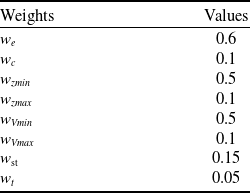
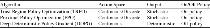


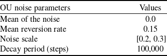

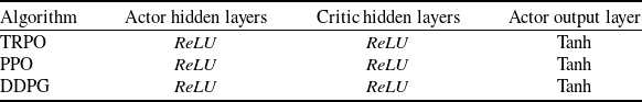
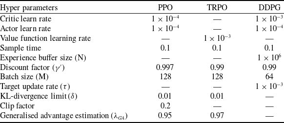
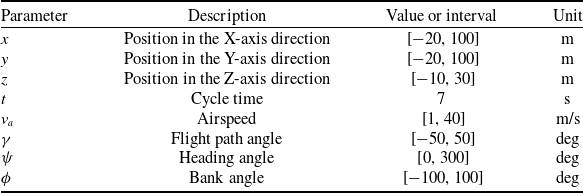


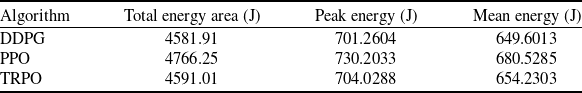


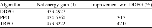
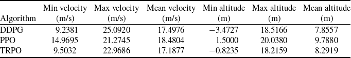


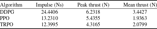


 Open access