2. Literature review

In terms of the effects of monetary policy on house prices, the early literature suggests a weak link between the two variables. Dokko et al. (Reference Dokko, Doyle, Kiley, Kim, Sherlund, Sim and Van Den Heuvel2011) use quarterly data from 14 OECD countries from 1970 to 2002 and obtain evidence that traditional channels of monetary policy accounted for little of the rise in housing markets and that monetary policy was then not the main factor causing the housing boom of the 2000s. Kuttner (Reference Kuttner2013) provides a thorough review of the early literature on the impact of interest rates on house prices and concludes that the effects are too small to explain the real estate booms in the US and elsewhere over the past decade. Luciani (Reference Luciani2015) estimates a structural dynamic factor model using US quarterly data from 1982 to 2010 and concludes that the contribution of the Fed’s expansionary monetary policy from 2002–2004 to the recent housing cycle was negligible.

Conversely, other studies find compelling evidence of a link between monetary policy and house prices. For example, Del Negro and Otrok (Reference Del Negro and Otrok2007) estimate a VAR model using US quarterly data from 1986 to 2005 and find that monetary policy shocks can explain a sizable share of housing price movements. Jarocinski and Smets (Reference Jarocinski and Smets2008) show that monetary policy has significant effects on housing investment and house prices and that easing monetary policy in 2002–2004 contributed to the boom in the housing market in 2004 and 2005. McDonald and Stokes (Reference McDonald and Stokes2013) employ the S&P Case–Shiller aggregate 10-city monthly housing price indices and find evidence consistent with the view that the Fed’s interest rate policy in the period 2001–2004 of pushing down the federal funds rate and keeping it artificially low was a cause of the house price bubble. Using data spanning 140 years of modern economies including the US, Jorda et al. (Reference Jordà, Schularick and Taylor2015) show that loose monetary conditions lead to booms in real estate lending and house price bubbles. Finally, Cooper et al. (Reference Cooper, Luengo-Prado and Olivei2016) demonstrate the nonnegligible effect of monetary policy on regional house prices across different US states. For international evidence of the link between interest rates and house prices, see also Iacoviello and Minetti (Reference Iacoviello and Minetti2003), Iacoviello and Minetti (Reference Iacoviello and Minetti2008), Goodhart and Hofmann (Reference Goodhart and Hofmann2008), Sá et al. (Reference Sá, Towbin and Wieladek2011), Bordo and Landon-Lane (Reference Bordo and Landon-Lane2014), Head and Lloyd-Ellis (Reference Head and Lloyd-Ellis2016), Nocera and Roma (Reference Nocera and Roma2018), Kishor and Marfatia (Reference Kishor and Marfatia2018), and Robstad (Reference Robstad2018). In general, based on the previous literature, use of a vector autoregressive (VAR) framework seems to provide more supportive evidence that loose monetary policy causes house price appreciation and that these impacts are significant and nonnegligible. This paper follows the same lines as the existing VAR literature but augments the VAR model with credit conditions, market sentiment, and time-on-the-market, which are also potentially important explanations of house price swings.

Table 1. Data source

Figure 1. Data.

Figure 2. Monetary policy shock.

Figure 3. Credit shock.

Regarding the channels that may work for monetary policy shocks, the role of credit is attracting attention after the crisis of 2008–2009 [see, e.g., Schularick and Taylor (Reference Schularick and Taylor2012); Iacoviello (Reference Iacoviello2015); Mian and Sufi (Reference Mian and Sufi2018)]. Most house buyers need to obtain mortgage loans for a home purchase, and typical households face borrowing constraints. Agnello et al. (Reference Agnello, Castro and Sousa2018) suggest that credit market conditions are crucial for housing market booms, whereas Rojas (Reference Rojas2021) provides evidence that growth in mortgage credit during the 1990s and mid-2000s was greatest for lower-income borrowers, which then led to the financial crisis of the mid-2000s. Using the lifting of branching restrictions that took place in the US after 1994, Favara and Imbs (Reference Favara and Imbs2015) demonstrate a causal chain going from an expansion in credit to house prices. Moreover, Mian and Sufi (Reference Mian and Sufi2021) argue that greater availability of credit leads optimistic speculators to increase demand and house prices. This increase in house prices may then convince more people to become speculators, which further boosts house prices. Hence, as expansionary monetary policy relaxes credit constraints, the credit channel tends to amplify and propagate the effects of monetary policy on house prices [see, e.g., Segev and Schaffer (Reference Segev and Schaffer2020)].

It is also argued that market sentiment plays a vital role in asset price dynamics. Bekiros et al. (Reference Bekiros, Nilavongse and Uddin2020) provide a theoretical framework to demonstrate how a rise in optimistic expectations about future house prices triggers housing market booms. Kaplan et al. (Reference Kaplan, Mitman and Violante2020) find that beliefs about future house prices, or expectations, are the key source of variation in home values and reveal that it was a shift in beliefs, not a change in credit conditions, that drove the US housing boom–bust around the time of the Great Recession. Whereas house prices reflect the present value of future cash flows or house rents, expectations of the future housing market indicate how those upcoming house rents may vary. Using questionnaire surveys of homebuyers, Case and Shiller (Reference Case and Shiller2003) and Case et al. (Reference Case, Shiller and Thompson2012) discover that expectations of a boost in future house prices play an important role in determining recent US house price booms. Lambertini et al. (Reference Lambertini, Mendicino and Punzi2013) and Ben-David et al. (Reference Ben-David, Towbin and Weber2019) also show that expectations of rising house prices explain a sizable proportion of the fluctuations in house prices. Lastly, Soo (Reference Soo2018) uses the news media to construct a sentiment index for house price expectations and finds that sentiment has significant predictive power for future house prices, and should then be taken seriously as a potential determinant of house prices, especially in research surrounding policy concerns.

Finally, several studies investigate the relationship between the time-on-the-market and house prices. As argued by Benefield and Hardin (Reference Benefield and Hardin2015), time-on-the-market is one of the most analyzed outcomes in the residential literature. Using meta-analysis, Sirmans et al. (Reference Sirmans, MacDonald and Macpherson2010) provide evidence that time-on-the-market has a negative impact on house prices, whereas Dube and Legros (Reference Dube and Legros2016) find evidence that houses staying longer on the market provide negative information to the market, which results in a lower final sale price.

3. Empirical strategy

To examine the linkage between house prices and monetary policy, we consider a stylized SVAR model of the housing market augmented with monetary policy, credit condition, and market sentiment:

(1) \begin{equation} A_0y_t= A_1 y_{t-1} + \cdots + A_p y_{t-p}+e_t, \end{equation}

where $y_t$ is a vector containing the federal funds rate, credit conditions, market sentiment, the log of housing loans, the housing inventory–sales ratio, and the log of real house prices. Following Bernanke and Blinder (Reference Bernanke and Blinder1992) and Bernanke and Mihov (Reference Bernanke and Mihov1998), the federal funds rate is the monetary policy instrument. General credit conditions indicate the availability and cost of borrowing for various purposes, including purchasing homes. Moreover, housing market sentiment is also an important determinant of house prices [see e.g., Soo (Reference Soo2018)]. We use housing loans to measure housing demand, and the housing inventory–sales ratio to reflect the time-on-the-market, i.e., housing market liquidity as a proxy of housing supply.

Figure 4. Sentiment shock.

Figure 5. Housing demand shock.

Figure 6. Housing supply shock.

The term $e_t$ denotes the structural shocks with mean zero and a diagonal variance–covariance matrix $\Lambda = E(e_t e'_{\!\!t})$ , where the diagonal entries are the variances of the structural shocks.

We estimate the reduced-form vector autoregressive (VAR) model using

(2) \begin{equation} y_t = \phi _1 y_{t-1} + \cdots + \phi _p y_{t-p} + u_t, \end{equation}

where $u_t$ denotes the regression errors. Note that the structural shocks and the reduced-form errors are related by $A_0 u_t= e_t$ , where $u_t=(u_{1t}, u_{2t}, u_{3t}, u_{4t}, u_{5t}, u_{6t})'$ is the vector of regression errors for each variable in equation (2). Regarding the structural shocks,

\begin{equation*} e_t = (e_t^{\text{MP}}, e_t^{\text{Credit}}, e_t^{\text{Sent}}, e_t^{\text{Demand}}, e_t^{\text{Supply}}, e_t^{\text{HP}})', \end{equation*}

where $e_t^{\text{MP}}$ represents a monetary policy shock, whereas $e_t^{\text{Credit}}$ , $e_t^{\text{Sent}}$ , $e_t^{\text{Demand}}$ , and $e_t^{\text{Supply}}$ are nonpolicy structural shocks, i.e., credit supply shocks, sentiment shocks, housing demand shocks and housing supply shocks, respectively. The residual shock $e_t^{\text{HP}}$ represents all other shocks affecting house prices without a particular structural interpretation.

We achieve identification by imposing a recursive restriction on $A_0$ . The key assumption is that monetary policy does not respond instantaneously to all other variables in the SVAR system. In particular, we assume that the Fed does not respond to house price movements in setting monetary policy within the month. This draws on existing empirical findings that the interest rate response to house price shocks in the US is statistically insignificant [see, e.g., Musso et al. (Reference Musso, Neri and Stracca2011)], and that the Fed tends to raise policy rates after a few quarters of housing demand shocks, i.e., a delayed response [Andre et al. (Reference Andre, Gupta and Kanda2012)].

In the second equation, given that credit conditions measure the general availability and cost of borrowing money for various purposes, we assume these do not respond to housing market-specific variables within the month and are only driven by monetary policy. Conversely, readily available and affordable credit can lead to increased speculative activity and investment in the real estate market, which may cause participants to become more optimistic about the housing market. Finally, easy access to credit for home buyers and home construction firms can also boost both housing demand and supply and therefore house prices.

In the third equation, housing market sentiment is driven by monetary policy and credit shocks, but there is a lagged response to housing market-specific shocks. This is motivated by the fact that the general economic and financial market outlook, including monetary policy and credit conditions, is frequently discussed in the media, and affects housing market sentiment in real time. In contrast, it may take time for the public to receive information about housing market conditions. Real estate market data, such as house prices or inventory levels, often take some time to be collected, analyzed, and reported. Therefore, individuals may not be immediately aware of the current state of the housing market, which should delay the effect on sentiment.

The fourth to sixth equations represent the housing market, where housing demand and supply shocks are identified. In addition to shocks from monetary policy, credit conditions, and market sentiment, positive housing demand shocks encourage increased home purchases with external financing, and thus impact upon housing loans. Moreover, both housing demand and supply shocks affect the housing inventory–sales ratio, i.e., the time-on-the-market. Higher demand creates a seller’s market in which home buyers act swiftly to secure their target property and reduces the average time a home remains on the market. Conversely, positive supply shocks lead to a longer time-on-the-market as properties take longer to sell in a buyer’s market. Finally, all types of shocks in the SVAR system affect house prices. After accounting for shocks to monetary policy, credit conditions, housing market sentiment, housing demand, and housing supply, we treat the shock in the house price equation as a residual shock unaccounted for in the model, which we simply denote as a house price shock.

It is worth noting that as the focus of the current paper is the effect of monetary policy shocks on house prices, the identification of the monetary policy shocks is more solid than those of any other structural shocks. Nevertheless, we later use impulse response analysis to check whether the responses of house prices are a plausible reaction to the various types of structural shocks.

4. Data

We use monthly data from 1978:M1 to 2019:M9. We assess credit conditions using the Credit Subindex of the Chicago Fed National Financial Conditions Index (NFCI), which provides a comprehensive update on US financial conditions in money markets, debt and equity markets, and the traditional and shadow banking systems. The credit subindex is composed of measures of credit conditions, where positive values of the index indicate tighter credit conditions than average, whereas negative values indicate looser credit conditions than average.

To proxy housing market sentiment, we use data from the Michigan Survey of Consumers (SOC), which has been applied to capture home buyer confidence [see, e.g., Piazzesi and Schneider (Reference Piazzesi and Schneider2009); Lambertini et al. (Reference Lambertini, Mendicino and Punzi2013)]. In the SOC, a nationally representative sample of 500 individuals is surveyed on their views about business and buying conditions, including questions about the housing market. The question is “[g]enerally speaking, do you think now is a good time or a bad time to buy a house?” and respondents answer “good time,” “bad time,” or “uncertain.” Letting $G_t$ and $B_t$ denote the percentage of respondents that respond “good time” and “bad time,” respectively, the SOC constructs the index of buying conditions for houses as follows:

\begin{equation*} \text{Sent}_t = 100 + (G_t-B_t). \end{equation*}

The index serves to measure housing market sentiment. It has been shown that the SOC index is highly correlated with the media housing sentiment index constructed by social media text mining [see, e.g., Soo (Reference Soo2018)], which validates the SOC index being a reliable measure of consumer optimism about house prices.

Table 2. Variance decomposition of real house prices

Figure 7. Historical decomposition.

Figure 8. Contribution of each structural shock to the cumulative change in the house prices during January 2002 to May 2006.

Figure 9. Instrumented monetary policy shock.

Figure 10. Time-varying VAR: response of house prices during different periods. (a) Impulse responses: house prices to monetary policy shocks in 1987:1, 1997:1, 2007:1, and 2017:1, (b) Difference between the responses in 1997:1 and 1987:1, with the 90% confidence interval, (c) Difference between the responses in 2007:1 and 1987:1, with the 90% confidence interval, and (d) Difference between the responses in 2017:1 and 1987:1, with the 90% confidence interval.

Figure 11. Unrestricted and counterfactual responses [Kilian and Lewis (Reference Kilian and Lewis2011)’s counterfactual].

Figure 12. Unrestricted and counterfactual responses [Bernanke et al. (Reference Bernanke, Gertler and Watson1997)’s counterfactual].

Figure 13. Response of house prices and test results of asymmetry.

Figure 14. Gilchrist and Zakrajsek (Reference Gilchrist and Zakrajsek2012)’s excess bond premium.

Figure 15. Bork et al. (Reference Bork, Møller and Pedersen2020)’s housing sentiment index.

Figure 16. New privately-owned housing units authorized in permit-issuing places: total units.

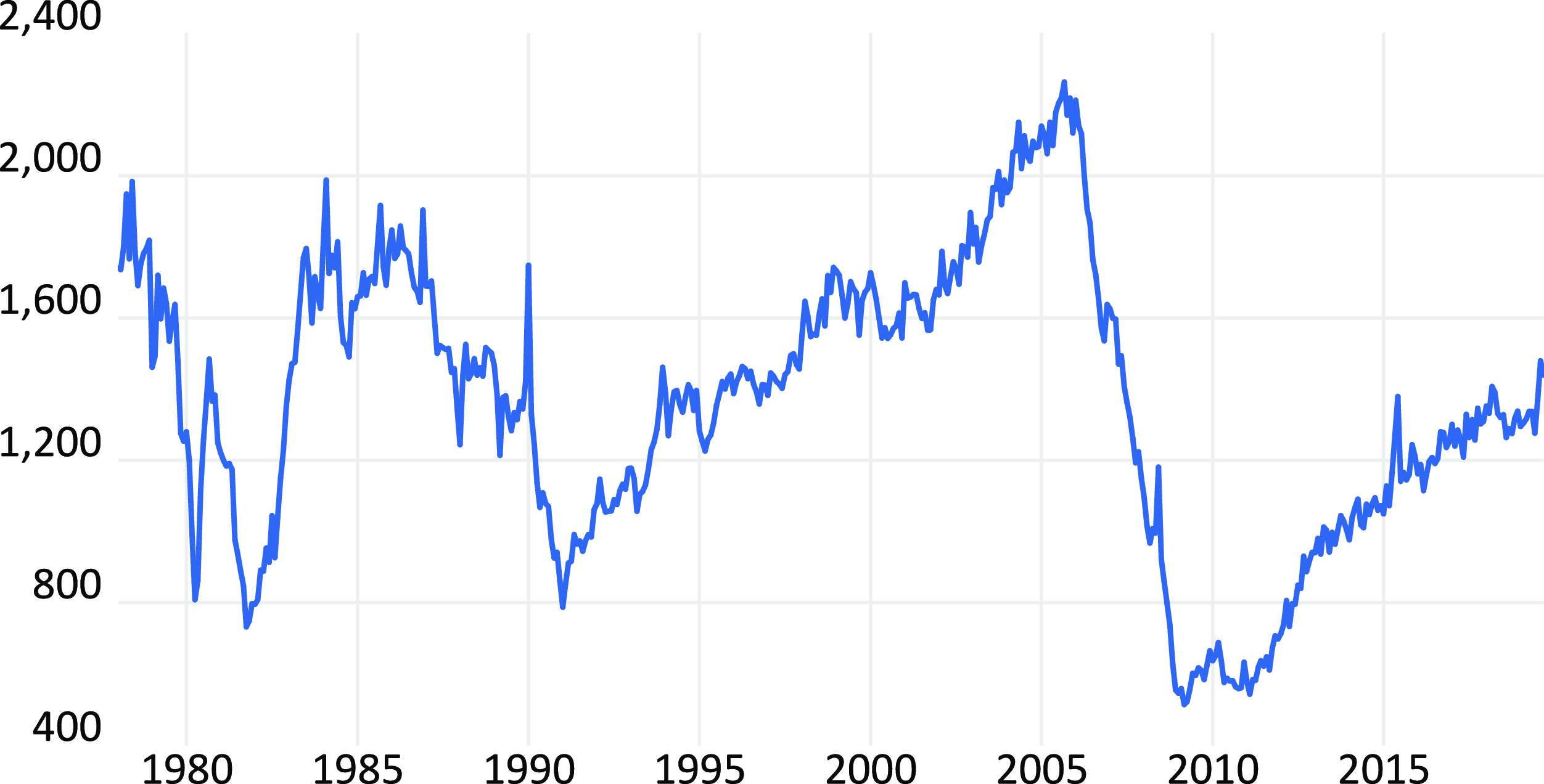
Figure 17. Wu and Xia (Reference Wu and Xia2016) shadow rates and federal funds rates.

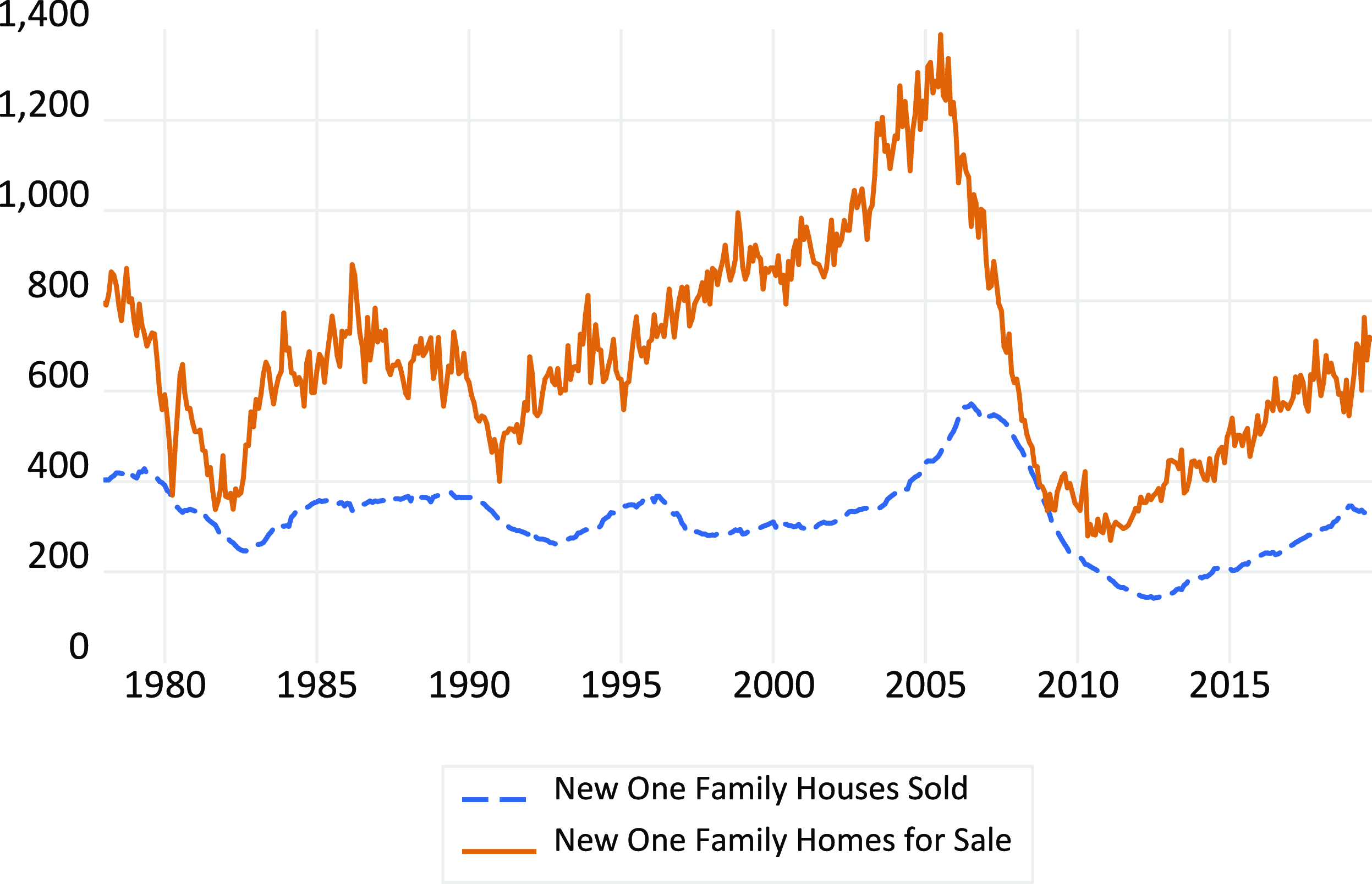
Figure 18. US new one family houses (sold and for sale).

We measure housing loans using all real estate loans (for all commercial banks) and construct the housing inventory–sales ratio by dividing houses for sale by houses sold. Because this provides an indication of the size of the for-sale inventory in relation to the number of houses currently sold, we can use it to measure the time-on-the-market, i.e., how long the current for-sale inventory would last given the current sales rate if no additional new houses were built. Finally, we use the S&P CoreLogic Case–Shiller home price index deflated by the consumer price index to measure real house prices.

Figure 19. Robustness 1, impulse response to monetary policy shocks.

Figure 20. Robustness 2, impulse response to monetary policy shocks.

Figure 21. Robustness 3, impulse response to monetary policy shocks.

Figure 22. Robustness 4, impulse response to monetary policy shocks.

Figure 23. Robustness 5, impulse response to monetary policy shocks.

All the data except the SOC index and the S&P CoreLogic Case–Shiller home price index are from the Federal Reserve Economic Data (FRED) constructed by the Federal Reserve Bank of St. Louis. The SOC index is from the Michigan Survey of Consumers, whereas the S&P CoreLogic Case–Shiller home price index is available from Robert Shiller’s webpage.Footnote ² All the data are described in Table 1 and the time series plots are shown in Figure 1.

5. Monetary policy and the US housing market

We first examine the impulse response functions to evaluate whether the SVAR model can characterize the cyclical properties of the US housing market. Our purpose is to check whether the responses of the house price are plausible reactions to the different types of shocks, and most importantly, whether monetary policy shocks have a significant impact on house prices. Whether these responses persist is also of interest. We select the lag length of the VAR model using the Akaike information criterion, although the Bayesian information criterion provides comparable results. We also use the structural forecast error variance decomposition to see if the monetary policy shock accounts for a considerable portion of the variation in house prices.

5.3. Monetary policy and the 2002–2006 US housing boom

It is claimed in Bernanke (Reference Bernanke2010) that the direct linkages between monetary policy and housing bubbles are weak, whereas Taylor (Reference Taylor2015) argues that the low-interest rate policy of 2003–2005 brought on a search for yield and was then a key factor in the subsequent financial crisis and the Great Recession. Here, we further address the question of whether loosening monetary policy causes house price booms during our sample period using historical decomposition. We construct the base projection of house prices, which is obtained from the VAR model without any stochastic shocks. We then perform a historical decomposition to dynamically simulate the model by turning on only one realized historical structural shock, with the other shocks set to zero. Hence, we can determine the importance of any one structural shock by examining the extent to which the introduction of the particular shock in house prices closes the gap between the base projection and the actual series. Figure 7 plots the cumulative contribution of different shocks to house prices. It is evident that we can historically explain a substantial portion of the movements in house prices using monetary policy shocks. By contrast, sentiment shocks have made comparatively small contributions to house prices.

It is of special interest to focus on the specific period between when the housing boom began in early 2002 and reached its record high in mid-2006.Footnote ³ Hence, we further examine whether we can attribute the house price hike during the period 2002–2006 to monetary policy shocks. Let $\hat{y}_{6t}^{j}$ denote the counterfactual house price series with only the realized historical shocks $j\in \{\text{MP, Credit, Sent, Demand, Supply, HP}\}$ , and $\text{base}_{6t}$ denote the base projection without any stochastic shocks. As discussed, we can measure the importance of structural shock $j$ by examining the extent to which the introduction of shock $j$ in house prices (i.e., $\hat{y}_{6t}^{j}-\text{base}_{6t}$ ) closes the gap between the base projection and the actual series (i.e., $y_{6t}-\text{base}_{6t}$ ). We thus follow the spirit of Kilian and Lee (Reference Kilian and Lee2014), and use the following measure to present the information conveyed by historical decomposition:

\begin{equation*} \text{HD}_{6,T_1,T_2}^{j} = 100\times \frac {(\hat {y}_{6T2}^{j}-\text{base}_{T2})-(\hat {y}_{6T1}^{j}-\text{base}_{T1})}{(y_{6T2}-\text{base}_{6T2})-(y_{6T1}-\text{base}_{6T1})} \end{equation*}

for $T_1\lt T_2$ . That is, the portion of the cumulative change in $y_{6t}-\text{base}_{6t}$ between dates $T_1$ and $T_2$ explained by structural shock $j$ .

A high value of $\text{HD}_{6,T_1,T_2}^{j}$ indicates that the gap between the base projection and the actual series can be largely explained by structural shock $j$ during the period between $T_1$ and $T_2$ . Alternatively, a negative value of $\text{HD}_{6,T_1,T_2}^{j}$ indicates that the impact of structural shock $j$ has been offset by the remaining shocks. We provide a bar chart to show $\text{HD}_{6,T_1,T_2}^{j}$ for different shocks during 2002:M1–2006:M5 in Figure 8. Using this, we can see that between 2002:M1 and 2006:M5, monetary policy shocks account for 69% of house price variations, which is the highest percentage among all the structural shocks. Hence, the results from the historical decomposition provide some indirect evidence to support the claim that the “too-low-for-too-long” interest rates starting in the early 2000s may have caused the subsequent US housing market booms.

5.5. External instrument identification

In our baseline results, we employ the federal funds rate as a measure of monetary policy, which is also influenced by forces other than monetary policy. To account for bias when estimating the effects of monetary policy using federal funds rates, the literature suggests the use of the narrative approach in Romer and Romer (Reference Romer and Romer2004) to construct an external series as a more exogenous measure of monetary policy shocks. As argued by Montiel Olea et al. (Reference Montiel Olea, Stock and Watson2021), while such an external series would not represent a genuine monetary policy shock, it can be treated as a variable plausibly correlated with monetary policy shocks, and uncorrelated with other structural shocks. Hence, in the spirit of Stock and Watson (Reference Stock and Watson2012) and many other recent works in the literature [see, e.g., Mertens and Ravn (Reference Mertens and Ravn2013); Gertler and Karadi (Reference Gertler and Karadi2015); Mertens and Montiel Olea (Reference Mertens and Montiel Olea2018)], this section aims to strengthen the argument for the impact of monetary policy shocks on house prices by incorporating identification with an external instrument, i.e., Romer and Romer’s series.

Table 3. Variance decomposition: percentage contribution of monetary policy shocks for different robustness specifications

Note: Robustness 1 represents the model using Gilchrist and Zakrajsek (Reference Gilchrist and Zakrajsek2012)’s excess bond premium as a measure of credit condition. Robustness 2 represents the model with the Bork et al. (Reference Bork, Møller and Pedersen2020)’s housing sentiment index. Robustness 3 represents the model using housing permits as a measure of housing demand. Robustness 4 represents the model using the Wu and Xia (Reference Wu and Xia2016) shadow rates as a measure of monetary policy. Robustness 5 represents the model using the ratio of the new one-family houses sold to new one-family homes for sale to measure the time-on-the-market.

Figure 24. Robustness: historical decomposition. Robustness 1 represents the model using Gilchrist and Zakrajsek (Reference Gilchrist and Zakrajsek2012)’s excess bond premium as a measure of credit condition. Robustness 2 represents the model with the Bork et al. (Reference Bork, Møller and Pedersen2020)’s housing sentiment index. Robustness 3 represents the model using housing permits as a measure of housing demand. Robustness 4 represents the model using the Wu and Xia (Reference Wu and Xia2016) shadow rates as a measure of monetary policy. Robustness 5 represents the model using the ratio of the new one-family houses sold to new one-family homes for sale to measure the time-on-the-market.

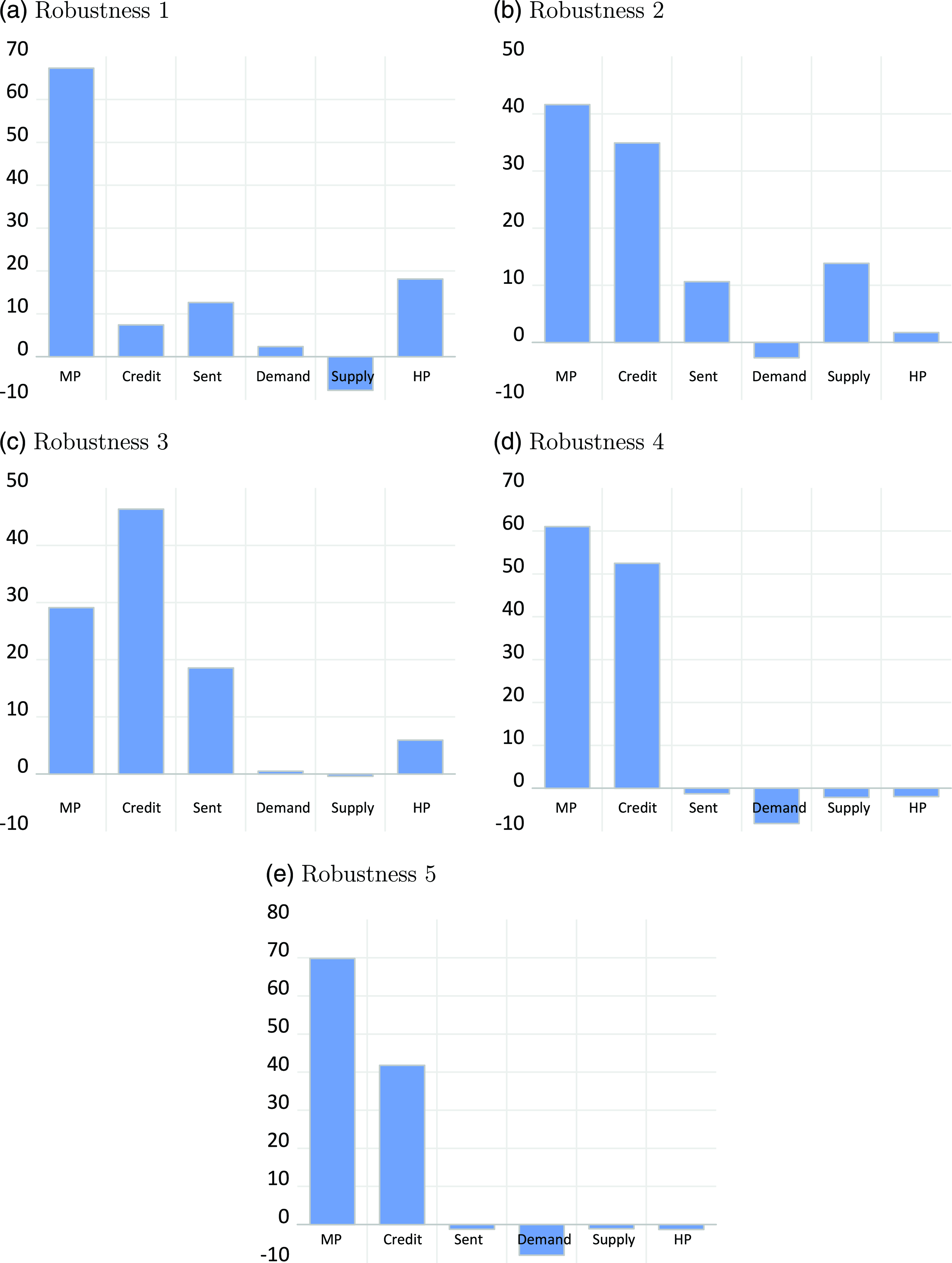
Figure 25. Robustness: contribution of each structural shock to the cumulative change in the house prices during January 2002 to May 2006. See notes to Figure 24 for more details about different robustness specifications.

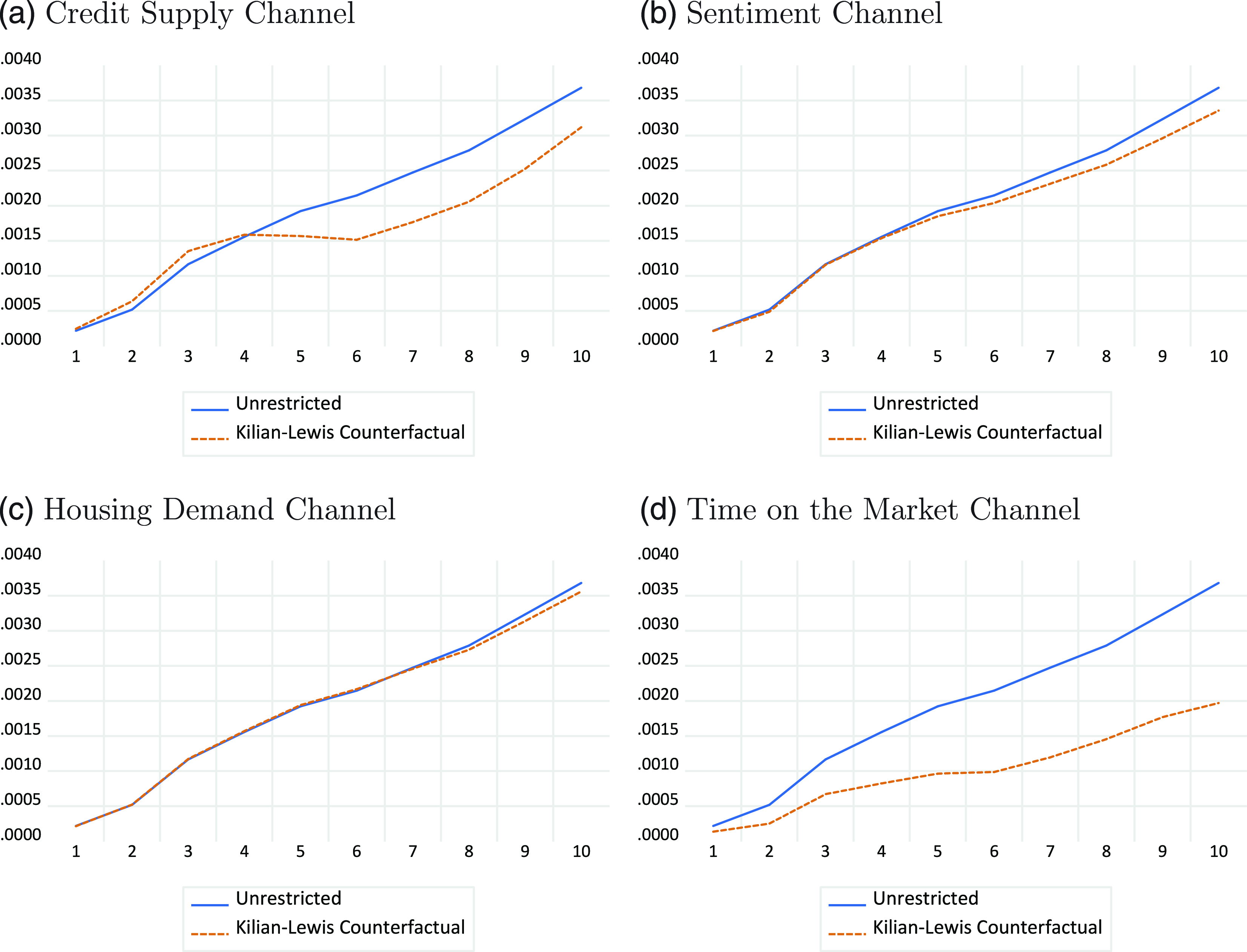
Figure 26. Robustness 1: Unrestricted and counterfactual responses [Kilian and Lewis (Reference Kilian and Lewis2011)’s counterfactual].

We employ the updated Romer and Romer (Reference Romer and Romer2004)’s series constructed by Miranda-Agrippino and Rey (Reference Miranda-Agrippino and Rey2020) and Miranda-Agrippino and Ricco (Reference Miranda-Agrippino and Ricco2021).Footnote ⁶ The identifying assumption underlying this approach is twofold: (1) the federal funds rate is correlated with the narrative instrument, and (2) the series of instrument is exogenous to other shocks in the system. These assumptions align with the methodological framework presented by Romer and Romer (Reference Romer and Romer2004). While the second assumption is not testable, we follow Montiel Olea et al. (Reference Montiel Olea, Stock and Watson2021) to address concerns regarding the instrument’s strength. The calculated Wald statistic for this analysis is 8.93, exceeding the critical value of 3.84 at a 95% confidence level, which supports the rejection of the null hypothesis of irrelevance.

Figure 9 presents the impacts of the monetary policy shocks on each variable, along with the 95% weak-instrument robust confidence interval proposed by Montiel Olea et al. (Reference Montiel Olea, Stock and Watson2021). Notably, the impulse responses displayed in the figure exhibit no qualitative deviations from our baseline findings. That is, the responses to the instrumented monetary policy shocks closely resemble those observed in the benchmark analysis. In sum, this exercise reinforces our initial conclusion about the significance of expansionary monetary policy causing a house price appreciation.

6. How important are the different channels for monetary transmission mechanism?

Because we have shown that monetary policy has a nonnegligible influence on house prices, it is of interest to investigate further how important the different channels are through which low-interest rates cause the housing market to boom. To respond to this question, we follow the approach proposed by Kilian and Lewis (Reference Kilian and Lewis2011) to conduct a counterfactual analysis, which they use to investigate how the monetary policy channel amplifies the effects of oil price shocks on real output.

Using the credit channel as an example, to quantify this channel, we consider a counterfactual in which credit conditions react to fluctuations in all variables in the SVAR model except the monetary policy shocks. To shut down the direct response of credit conditions to monetary policy shocks, we construct a sequence of hypothetical shocks to credit conditions that offset the contemporaneous and lagged effects of the federal funds rate on credit conditions.

We only shut down the response of credit conditions to monetary policy shocks, and allow credit conditions to respond to the other endogenous variables in the SVAR model, i.e., the response of credit conditions need not be zero. Hence, we can use the difference between the unrestricted (actual) and counterfactual impulse responses to quantify the effects of monetary policy shocks on house prices through the credit condition. A large gap between these two responses suggests the credit channel plays an important role in the transmission of monetary policy. By contrast, if the actual and counterfactual responses are close to each other, we would conclude that credit conditions do not act as a channel for monetary policy. We can quantify alternative channels such as the market sentiment, housing demand, and time-on-the-market channels using an analogous procedure.

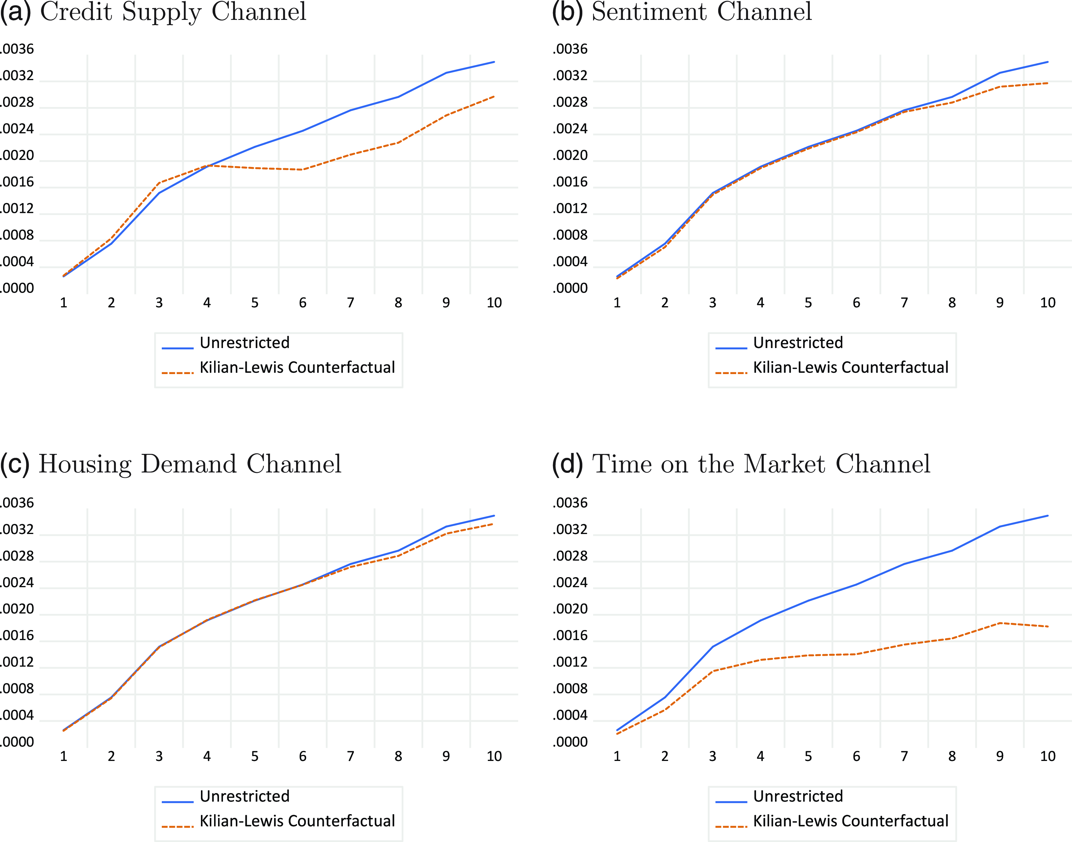
Using the case of an expansionary monetary policy shock, Figure 11 illustrates the counterfactual results for the different channels. The solid line represents the unrestricted response of house prices to a loose monetary policy shock, whereas the dashed line represents the counterfactual responses. The difference between the two lines indicates the effects of the channels. According to Figure 11, the most important channel is the time-on-the-market channel, whereby faster sales and lower inventory levels in the housing market amplify the effects of an expansionary monetary policy shock. The credit channel also plays a role in the transmission of monetary policy shocks to house prices. However, in the absence of the sentiment and housing demand channels, the responses of house prices are precisely the same as they were. This implies that the sentiment and housing demand channels are not important in the transmission of monetary policy shocks.

It is worth noting that we can construct an alternative counterfactual approach by holding channel variables such as credit conditions, market sentiment, housing loans, and the inventory–sales ratio fixed in response to monetary policy shocks [see, e.g., Bernanke et al. (Reference Bernanke, Gertler and Watson1997)]. This alternative approach is called the Bernanke–Gertler–Watson (BGW) counterfactual by Kilian and Lewis (Reference Kilian and Lewis2011).

Figure 12 depicts the BGW counterfactuals with the unrestricted responses, and provides similar results to the Kilian and Lewis (Reference Kilian and Lewis2011) approach. The time-on-the-market remains the most crucial channel for monetary policy transmission.

Figure 27. Robustness 2: Unrestricted and counterfactual responses [Kilian and Lewis (Reference Kilian and Lewis2011)’s counterfactual].

7. Do monetary policy shocks have asymmetric effects on house prices?

In this section, we further investigate if the effects of monetary policy shocks on house prices are asymmetric. A strand of previous empirical studies tends to find that monetary contractions have a significantly greater effect on economic activity than an equally sized expansionary policy [see, e.g., DeLong and Summers (Reference DeLong and Summers1988); Cover (Reference Cover1992); Rhee and Rich (Reference Rhee and Rich1995); Karras (Reference Karras1996); Karras and Stokes (Reference Karras and Stokes1999); Tenreyro and Thwaites (Reference Tenreyro and Thwaites2016); Angrist et al. (Reference Angrist, Jordà and Kuersteiner2018)]. Following Tenreyro and Thwaites (Reference Tenreyro and Thwaites2016), we use the local projection method proposed by Jorda (Reference Jorda2005) to investigate further whether positive and negative shocks to policy rates have different impacts on house prices, $y_t$ :

(3) \begin{equation} y_{t+h} = \alpha _h + \beta _h^+\times \max\![e_t^{\text{MP}},0] + \beta _h^-\times \min\![e_t^{\text{MP}},0] + \gamma'_{\!\!h}\boldsymbol{x}_t + \varepsilon _{t+h}, \end{equation}

where $\max\![e_t^{\text{MP}},0]$ and $\min\![e_t^{\text{MP}},0]$ are contractionary and expansionary monetary shocks and $\boldsymbol{x}_t$ is a vector of controls including one lag of the dependent variable and other structural shocks.

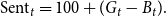
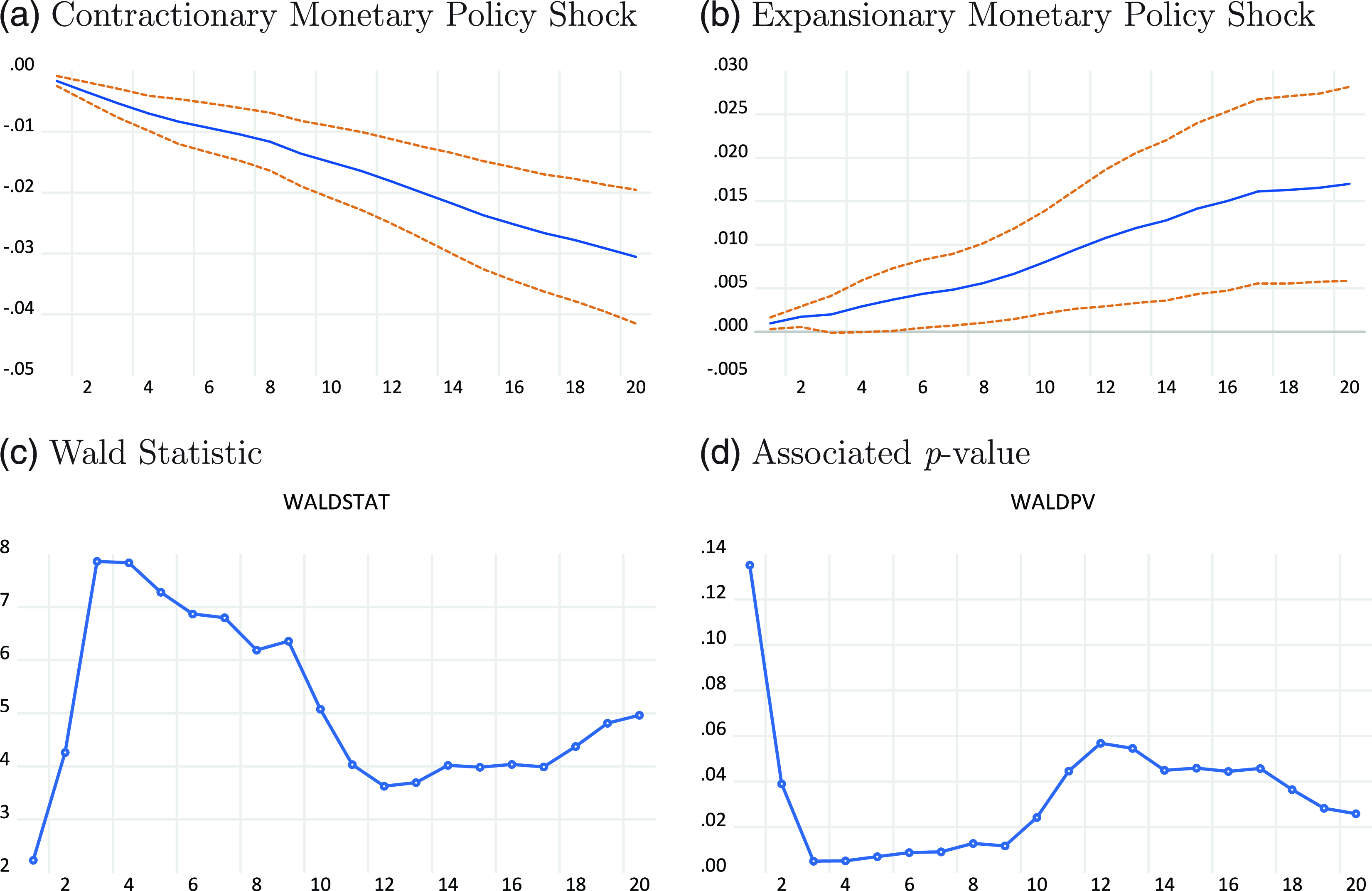
Figure 13(a) and (b) plots the impulse responses of house prices for positive and negative policy rate shocks, respectively. As suggested by Jorda (Reference Jorda2005), we construct a 95% confidence interval using the Newey–West heteroskedasticity and autocorrelation consistent (HAC) estimator. As expected, a positive (contractionary) shock causes house prices to decrease, whereas a negative (expansionary) shock causes house prices to increase. Both responses are statistically significant. Moreover, the magnitudes of responses are much higher for interest rate hikes than cuts, which suggests that the effects of monetary policy shocks on house prices are indeed asymmetric. The Wald statistics and associated $p$ -values for testing the null hypothesis $H_0\;:\; |\beta _h^+| = | \beta _h^-|$ , $h=0,1,\ldots,H$ , are in Figure 13(c) and (d). Clearly, we can reject the null hypothesis over most horizons, which provides convincing evidence of asymmetry.

Figure 28. Robustness 3: Unrestricted and counterfactual responses [Kilian and Lewis (Reference Kilian and Lewis2011)’s counterfactual].

Figure 29. Robustness 4: Unrestricted and counterfactual responses [Kilian and Lewis (Reference Kilian and Lewis2011)’s counterfactual].

Figure 30. Robustness 5: Unrestricted and counterfactual responses [Kilian and Lewis (Reference Kilian and Lewis2011)’s counterfactual].

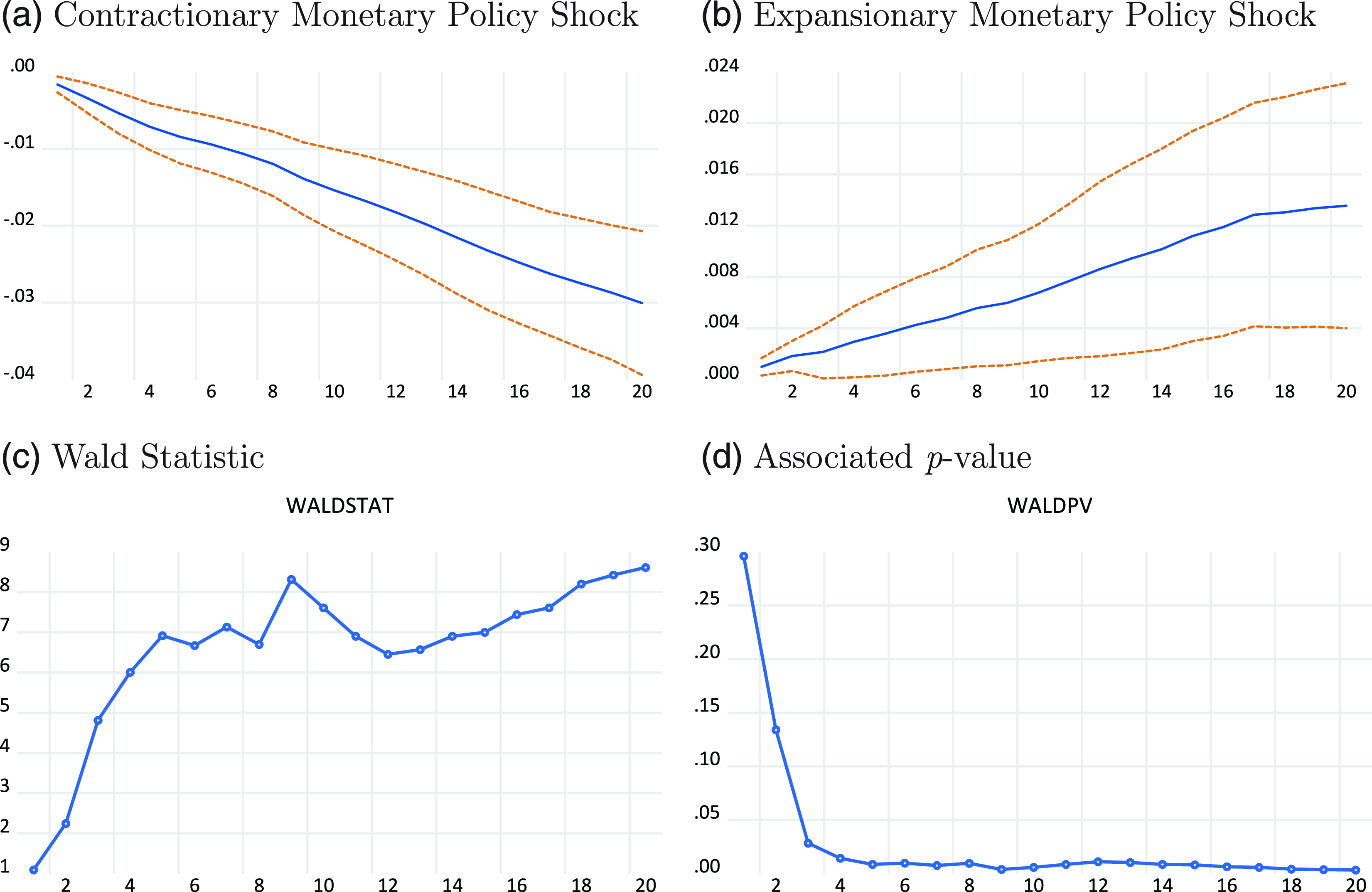
Figure 31. Robustness 1: Response of house prices and test results of asymmetry.

Figure 32. Robustness 2: Response of house prices and test results of asymmetry.

Figure 33. Robustness 3: Response of house prices and test results of asymmetry.

Figure 34. Robustness 4: Response of house prices and test results of asymmetry.

Figure 35. Robustness 5: Response of house prices and test results of asymmetry.

8. Robustness

In this section, we provide a battery of robustness checks to validate our results from the baseline model. We first consider an alternative measure of credit conditions. Gilchrist and Zakrajsek (Reference Gilchrist and Zakrajsek2012) propose the use of the excess bond premium (EBP) as a measure of credit supply shocks, arguing that the proposed measure can capture exogenous variation in the pricing of default risk and as such constitutes an appropriate proxy for credit supply. They show that the EBP is highly correlated with measures of supply derived from the senior loan officers survey. In what follows, we replace the credit subindex of the Chicago Fed NFCI with the EBP in Gilchrist and Zakrajsek (Reference Gilchrist and Zakrajsek2012). The EBP data are updated by Favara et al. (Reference Favara, Lewis and Zakrajsek2016), and plotted in Figure 14.Footnote ⁷ We refer to these results as Robustness 1.

Second, a recent analysis by Bork et al. (Reference Bork, Møller and Pedersen2020) constructs a new measure of housing sentiment using household survey responses to questions about buying conditions for houses. Although the new measure is based on the same data source from the consumer surveys of the University of Michigan as in our baseline model, the authors refined the survey data using partial least squares to construct a housing sentiment index, which is argued to extract the most valuable information from the survey responses into an easy-to-interpret index of housing sentiment. Bork et al. (Reference Bork, Møller and Pedersen2020)’s housing sentiment index is available at a quarterly frequency,Footnote ⁸ and we thus convert the quarterly data into monthly data by the local quadric polynomial where the average of the monthly data matches the quarterly data. We plot Bork et al. (Reference Bork, Møller and Pedersen2020)’s housing sentiment index in Figure 15 and refer to the results as Robustness 2.

Third, an alternative measure of housing demand is used. Although future housing supply relates to the granting of building permits, it may also reflect a shift in current housing demand. We thus replace the housing loan data with building permits to identify housing demand shocks. The building permit data are the new privately owned housing units authorized in permit-issuing places (total units), which are available from the FRED. We plot the data for building permits in Figure 16, with the results denoted as Robustness 3.

Fourth, we account for the period of zero lower bound (ZLB) interest rates. In this analysis, we use the federal funds rate to reflect monetary policy. However, during the ZLB period, it is possible that the federal funds rate is unable to capture the features of monetary policy because it is almost always only slightly higher than zero. To address this concern, we replace the federal funds rate with the Wu–Xia shadow rate from 1990:M1 to 2019:M9 following Wu and Xia (Reference Wu and Xia2016). The Wu–Xia rate is estimated based on the idea of the shadow rate proposed by Black (Reference Black1995) and provides an alternative indicator of the Federal Reserve’s policy stance when the federal funds rate approaches the ZLB. As a reference, the rates are posted and updated by the Federal Reserve Bank of Atlanta on a regular basis. Figure 17 plots the differences between the federal funds rate and the Wu–Xia shadow rate. We title this exercise Robustness 4.

Finally, we consider an alternative measure of the time-on-the-market by calculating the ratio of new one-family houses sold to new one-family homes for sale. Both data are obtained from the FRED and plotted in Figure 18. Empirical results using the new measure of the time-on-the-market are denoted as Robustness 5.

The impulse response functions in response to an expansionary monetary policy are presented in Figures 19–23 for Robustness 1–5. Clearly, our baseline results remain: a loose monetary policy causes real house prices to significantly increase.

Moreover, the variance decomposition shown in Table 3 reveals that monetary policy shocks continue to explain about 23%–38% of the movements in real house prices. Figure 24 illustrates the historical decomposition results for our different robustness checks, which again align with our baseline results. In particular, Figure 25 also provides evidence that monetary policy shocks are responsible for the 2002–2006 US housing booms.

As for the transmission channels of monetary policy, Figures 26–30 suggest that while the credit supply channel may again have played some role consistent with the baseline findings, the time-on-the-market is unambiguously the most important channel amplifying the effects of monetary policy on house prices. Finally, Figures 31–35 suggest that our baseline evidence for the asymmetric effects of monetary policy shocks on house prices remains robust.