


1 Introduction
Traditionally, analytical studies of glacier and ice-sheet flow have considered length scales in the downstream direction which are either much shorter or longer than the thickness of ice. The former corresponds to classical models of basal sliding (e.g. Reference NyeNye, 1969, and particularly Reference FowlerFowler, 1979, Reference Fowler1981), while the latter leads to the shallow-ice approximation (e.g. Reference HutterHutter, 1983). A consistent model which deals with ice flow over basal undulations whose wavelengths are comparable with ice thickness is, however, desirable as it could elucidate how large obstacles such as drumlins and other glacial bedforms generate “form drag”.
Here we present a two-dimensional model for rapid ice flow over such large-wavelength obstacles (i.e. of lengths comparable to ice thickness). We restrict ourselves to the case where these obstacles play a significant role in the force balance of the ice flow, analogous to classical basal sliding. Given a stress tensor σ and a bed z = H(x) with normal n and tangent t (cf. Fig. 1), the force exerted by a section of bed on the body of ice is

where the integral is taken over the section of bed in question and ds denotes an element of arc of the bed. In classical hard-bed sliding, local basal shear stress t · σ n | z=H is usually assumed to be negligible due to the presence of a continuous regelation film. A thin weak layer of deforming sediment (e.g. Reference Engelhardt and KambEngelhardt and Kamb, 1998) under an ice stream could have a similar effect; moreover, it might suppress small-scale roughness generated by small obstacles such as clasts, as these would be sheared along with the till matrix. It is, however, conceivable that sufficiently large obstacles such as drumlins may contribute to force balance in the downstream direction through the first term on the righthand side above, which we have referred to as “form drag”. The theory constructed in sections 2–5 assumes that form drag is significant, and the scalings introduced in section 4 reflect this. Consequently, our theory is an extension of classical basal sliding theory to finite ice depth. We do not, however, ignore the possibility of small-scale roughness or local basal shear stress due to sediment deformation, but merely assume that basal “friction” due to these terms does not dominate over the effect of large-scale bed topography in determining flow velocities. This will be the case for a given bed topography if basal “friction” is sufficiently small, or, for a given local sliding law, if bed topography has sufficient amplitude. An analogous approach was previously taken in classical sliding theory by Reference MorlandMorland (1976b) and Reference FowlerFowler (1981).
Geometry of ice flow problem.

Certain restrictions on mean bed and surface slope (cf. sections 4 and 5) do, however, have to be applied to our theory; essentially the mean surface slope of the ice body has to be much smaller than the local bed roughness slope, which in turn is small compared with unity. This would obviously apply to drumlin-type basal topography under an ice stream; consequently most of the subsequent discussion refers to ice streams. While there is no unambiguous evidence that drumlins or other bedforms exist under present-day ice streams, geological evidence suggests that rapid sliding did occur over drumlinized terrain, for instance in the Puget Sound area (U.S.A.) during the last Ice Age (e.g. Reference Brown, Hallet and BoothBrown and others, 1987).
Reference MorlandMorland (1976a) was the first author to try to include the notion of finite ice depth in a theory of basal sliding. However, his solution of the flow equations does rely on a half-space (infinite depth) geometry, and he does not deal with perturbations caused at the glacier surface by bumps on the bed. Moreover, the ice-flow geometry considered by Morland is an inclined slab, whereas we consider a general ice-stream geometry and show explicitly how to separate the local flow problem over basal topography from the problem of the bulk flow of the ice stream; this may be seen as analogous to the asymptotic matching procedure of Reference FowlerFowler (1979, Reference Fowler1981), which relates the local basal sliding problem to the problem of bulk glacier flow. In the present case, however, the separation of the two flow problems is considerably more involved since they cannot be separated geometrically into a boundary layer and an outer flow. Instead, a more complicated multiple-scales approach must be used.
The assumption of significant form drag sets this analysis apart from those of Reference Gudmundsson, Raymond and BindschadlerGudmundsson and others (1998), who studied the effect of basal perturbations on ice-stream surfaces, of Reference MorlandMorland (2000), who considered basal undulations under ice sheets, and those of other authors who have considered the effect of basal perturbations on finite-depth ice flow (e.g. Reference Hutter, Legerer and SpringHutter and others, 1981; Reference HutterHutter, 1983; Reference ReehReeh, 1987). All of these authors consider perturbations to a basic shearing flow, where form drag is a higher-order correction, whereas our analysis assumes that form drag is of leading order. Indeed, our model may be applied to the case where there is no small-scale roughness and hence no “sliding law” in the classical sense, whereas Reference Gudmundsson, Raymond and BindschadlerGudmundsson and others (1998) and Reference MorlandMorland (2000) require a sliding law to be prescribed. However, as both Reference Gudmundsson, Raymond and BindschadlerGudmundsson and others (1998) and the present paper consider rapid ice flow over basal topography, some of the results obtained are similar. As we point out in section 3, the two models basically differ in assumptions about the size of basal obstacles and of basal shear stresses.
A two-dimensional model, by its very nature, has to neglect lateral shear (e.g. Reference Whillans and van der VeenWhillans and Van der Veen, 1997). However, as lateral shear is unlikely to vary over distances comparable with ice thickness (since ice streams are much wider than thick), this neglect is tantamount to ignoring a constant term in the local force balance, or equivalently, to overestimating the driving stress.
2 Model
The geometry of the problem is illustrated in Figure 1. We consider the flow of Newtonian viscous ice over a prescribed bed z = H(x), while z = D(x, t) denotes the upper surface of the ice. Given viscosity η, density ρ and acceleration due to gravity g and denoting the velocity field by u = (u, w), we obtain the usual slow-flow equations


where k is the z-unit vector. At the surface z = D, we prescribe vanishing shear and normal stress,


while the evolution of D(x, t) is governed by a kinematic boundary condition (where accumulation is ignored)

At the base of the ice stream z = H, we suppose that there may be an applied shear stress τ b (u b, x) which is a function of basal sliding velocity u b and position x,


τ b may arise if there is some microscale roughness or if there is a thin deforming sediment layer with sufficient shear strength. For a bed with no small-scale resistance, we simply put τ b = 0. Lastly, we have a kinematic boundary condition analogous to Equation (5) where basal melt is ignored,

3 Gudmundsson’s Model
Reference Gudmundsson, Raymond and BindschadlerGudmundsson and others (1998) assume that both z = H and z = D are straight, parallel lines inclined at some angle α to the horizontal, and then perturb them slightly (see Fig. 2; in fact, it is convenient to realign the coordinate system with these straight lines). A linearization of the equations in the previous section (with a particular choice of sliding law τ b) is then performed on the basis that the perturbations introduced are small.
Problem considered by Reference Gudmundsson, Raymond and BindschadlerGudmundsson and others (1998).

A crucial point, however, is that small geometrical perturbations may in fact introduce O(1) or even large perturbations into the stress field when sliding is rapid. To understand this, consider a bed perturbation of size h and wavelength D (scales for bed bump height and ice thickness, respectively) in Equation (8). Vertical velocity is then perturbed by an amount w ∼ u b h/D by such a bump. If this perturbation is of O(1) compared with the unperturbed shearing velocity in the ice u s, then a linearization of boundary condition (7) may fail, depending on the form of τ b in Equation (8). It is easy to see that, if sliding is rapid in the sense that ub /u s ≫ 1, w ∼ u s occurs for fairly subdued bumps, namely, when h/D ∼ u s/u b. Reference Gudmundsson, Raymond and BindschadlerGudmundsson and others (1998) estimate u b/u s at around 5000 for a typical ice stream, so w ∼ u s corresponds to h ≈ 0.2 m when D = 1000 m. If w is large compared with u s — and the previous argument indicates that this may in fact be the case when h is still quite small — then we may see terms in Equation (7) become important which are neglected, regardless of the choice of τ b, in Gudmundsson and others’ linearization. These terms include the “normal stress” effects which lead to form drag in classical basal sliding theory, and the rest of this paper is concerned with the situation where they are important.
4 Non-Dimensionalization
We define the following scales (see Fig. 3): [D] for the mean thickness of the ice stream (and also for the mean variation in bed elevation over the length of the ice stream), [L] for the length of the ice stream, [U] for a typical basal sliding velocity and [u] for typical internal deformation velocities (note that [U] and [u] are distinct and may be asymptotically different). Moreover, we suppose that there are bumps of wavelength ∼ [D] and amplitude [h] on the bed, and corresponding perturbations of height [d] to the ice-stream surface. [τ] will denote a typical deviatoric stress, while [τ d] is a scale for the driving stress, distinct from [τ]. Note that, because we scale the change in bed elevation H over the length of the ice stream L with [D], these scalings would not apply to a steep glacier geometry.
Scales for the ice-stream flow problem.

As in shallow-ice theory, the mean surface slope of the ice stream is assumed to be small,

There are then two important asymptotically different horizontal length scales, [D] and [L].We are mostly interested in the local flow problem on the short length scale [D], but the driving stress arises only because there is a mean decrease in surface elevation in the downstream direction over the length of the ice stream. One cannot therefore ignore variations on the long scale entirely, and this suggests multiply scaled horizontal coordinates and associated time variables


(x ⋆, t ⋆) and (X ⋆, T ⋆) are, of course, not independent, as (X ⋆, T ⋆) = ∊(x ⋆, t ⋆). In the limit ∊ ≪ 1 one can, however, treat them as independent in the context of a multiple-scales expansion (e.g. Reference HolmesHolmes, 1995). The “inner” variables (x ⋆, t ⋆) can be thought of as describing local variations, whereas the “outer” ones (X ⋆, T ⋆) describe the bulk behaviour of the ice stream. The appropriate transformation of derivatives is then


In his account of classical sliding, Reference FowlerFowler (1981) separated bed elevation into a smoothed bed and a local roughness component. Following his example, we define a smoothed bed elevation as a running average:

where [D] ≪ L M ≪ [L] so that the smoothed bed thus defined depends only on the outer variable X ⋆. Implicit in this definition is the assumption that basal topography occurs on asymptotically distinct length scales [D] and [L] with insignificant topography of intermediate wavelengths, which makes the smoothing above unique (cf. also Reference FowlerFowler, 1981). In practice, one might choose for L M the geometric mean of [D] and [L], L M = ([D][L])1/2 ≈ 20 km for a typical ice stream. It is expedient to apply a similar smoothing procedure to surface elevation and velocity, thus


These decompositions allow the following dimensionless variables to be defined in addition to Equations (11) and (12):


where i and k are the x- and z-unit vectors, respectively. The decompositions of u and p introduced here may seem overelaborate at first sight; they do, however, lead to some convenient simplifications later.
For a given ice-stream geometry, one can estimate the thickness and length scales [D] and [L] and the roughness scale [h]. It remains to define the other scales in terms of these. Clearly, the driving stress is

If the aspect ratio of a typical local bed bump is defined as

then the assumption that form drag in Equation (1) is a significant term in force balance suggests that (cf. Reference FowlerFowler, 1981)

If basal bumps are shallow with v ≪ 1, as will be assumed, then [τ] ≫ [τ d] and hence deformational velocities will be much greater than any shearing velocities due to the driving stress (u s defined in section 3) . This explains why both components of the local “deformational” part of the velocity field are scaled with [u] in Equation (19), and Equation (9) suggests we put

But [τ] is a typical deviatoric stress, and so we have

Combining Equations (26–28) gives us [U] and [u]:

Note that this derivation assumes that [U] is determined primarily by form drag, and not by the sliding law τ
b (u
b, x). In other words, the scaled basal shear stress  must be O(1) (or small) for all x and the value of [U] calculated here.
In a more realistic model, one might use a Glen’s law rheology  with an exponent n rather than a fixed η, and replace Equation (28) by [τ] = A
−1/n
([u]/[D])1/n
, from which one obtains
with an exponent n rather than a fixed η, and replace Equation (28) by [τ] = A
−1/n
([u]/[D])1/n
, from which one obtains

Using [τ d] = 104 Pa, [D] = 1 km, n = 3, A =10−24 s−1 Pa−3 and [h] = 50 m (as a representative drumlin height scale), one obtains [U] ≈ 5 km a−1, which is clearly about an order of magnitude too large for the Siple Coast ice streams (which have low driving stresses of ∼ 104 Pa), suggesting that glacial bedforms are unlikely to generate significant form drag. However, as drumlins usually have steep upstream faces, and the estimate (27) is based on approximating the local bed slope by v, the value of v = 0.05 may in fact underestimate the effect of bedforms. This is significant because [U] in Equation (30) depends strongly on v; with the values above but v = 0.1 instead of 0.05, we find [U] ≈ 315 m a−1. Moreover, we find in section 7 that even a conservative estimate of v can give rise to realistic sliding velocities.
It remains to fix [d], the scale for surface perturbations. Two mechanisms affect how large surface perturbations will be. Firstly, advection in Equation (6) suggests

and, secondly, hydrostatic pressure changes in Equation (5) would lead to

For a consistent model, one should choose the smaller choice of [d] above. For the present we choose Equation (31), and consider later in section 5.2 the rescaling required when ∊/v ≪ v.
5 Multiple-Scales Expansion
The scaled variables defined in the previous section are substituted in the model in section 2, and we omit the asterisks for convenience. All dependent variables other than H, D and U are assumed to depend on both inner and outer variables, which we treat as independent. In order that ordering in a multiple-scales expansion be preserved uniformly with respect to the inner variables, dependent variables must be bounded functions of the inner variables, x and t in our case. Furthermore, the averaging procedures (15–17) now yield


The dimensionless model contains two small parameters, v and ∊. We shall assume that ∊ ≪ v ≪ 1, and construct a leading-order model on this basis. The assumption that ∊ ≪ v is clearly realistic for most glacial bedforms; moreover, it ensures that deviatoric stresses [τ] = ρg[D]∊/v are much smaller than hydrostatic pressures ρg[D]. If this were not the case, one would expect widespread cavitation even in the absence of pressurized subglacial water.
As the boundaries of the ice-flow domain are z = H + vh and z = D + vd and v ≪ 1, the boundary conditions are expanded in Taylor series about z = H and z = D under the assumption that the flow field is sufficiently smooth to allow expansion to the required order. This approach can also be found in Reference NyeNye (1969) and Reference MorlandMorland (1976a, b), and allows the problem to be considered on the simpler domain H < z < D.
51 Expansion and simplification
To the error indicated, the scaled field equations become


while boundary conditions (4) and (5) at the surface are


In Equation (6) u| z =D+vd and w| z =D+vd are expanded inTaylor series to some order n about z = D

and at the base:


In Equation (9), we expand in a similar manner to Equation (40) above,

Equations (40) and (43) are simplified by introducing an averaging operator as

for any f for which 〈f〉 is well defined. Note that 〈f〉 = F for any F independent of x (essentially the smoothed quantities U, D and H), and from Equations (33) and (34), 〈d〉 = 〈h〉 = 0. Moreover, if f is bounded with respect to x, then

Where  in the usual notation. Armed with these properties of 〈·〉, we are now ready to manipulate Equations (40) and (43). Now, from Equation (43)

By integration by parts,

The first term on the righthand side vanishes by Equation (45). Therefore, by Equation (37)

Substituting Equation (48) in Equation (46) and using the properties of 〈·〉 listed above yields

if, formally, an integer n exists such that vn +1 ≲ ∊, and the expansions in Equations (40) and (43) can be carried out to this order.
Applying 〈·〉 to both sides of Equation (37) and using Equation (45) yields

and so 〈w〉 = O(∊) for all z.
In an anologous manner to the derivation of Equation (49), applying 〈·〉 to both sides of Equation (40) and manipulating yields

which leads to the conclusion that D depends only on the outer time variable T to O(∊), so D = D(X, T) to O(∊); this is hardly surprising since one would expect the mean thickness of the ice stream to change on the convective time-scale associated with its length (and not its thickness). Moreover, if we define  as an average in time analogous to the spatial average 〈·〉, then Equation (51) reduces to the familiar plug-flow mass conservation equation for D,

Equation (51) substituted back in Equation (40) yields the kinematic boundary condition

52 Leading-order model
Dependent variables are expanded as u = u 0 + O(v), d = d 0 + O(v), etc. This yields the following leading-order (to an O(v) error) model.


on the domain H < z < D 0, which is a semi-infinite strip with respect to the inner coordinates, as H and D only depend on the outer ones, X and T, to leading order. Note that, to leading order, we have a non-shearing flow; this is again analogous to classical sliding with shallow bed slopes (e.g. Fowler, Reference Fowler1986), and arises because [τ] ≫ [τd ].
From Equations (38) and (39), boundary conditions are


and from Equation (52)

while from Equations (41) and (43) one obtains


Note that, because the flow is non-shearing and [τ] ≫ [τ d], there is zero basal shear stress at leading order in Equation (58); τ b in Equation (38) is a O(v) correction.We should also comment at this point about the O(v 2/∊) term in Equations (39) and (56); its retention as a possible O(1) term is justified since, by virtue of ∊ ≪ v, we have v 2/∊ ≫ v. Hence the O(v 2/∊) term is much greater than the O(v) error in the leading-order model. We wish to retain the term explicitly because, as will be seen in the next section, it is responsible for the relaxation of surface perturbations to their steady-state shape. There remains the possibility that v 2/∊ ≫ 1, in which case a rescaling becomes necessary. This rescaling, d ⋆⋆ = (v 2/∊)d ⋆, introduces no new terms into the leading-order model, and the error remains of O(v). The rescaling converts Equations (56) and (57), respectively, into (again dropping asterisks)


One may then wish to ignore the O(∊/v 2) terms on the left-hand side in Equation (61). This is a singular perturbation, as it ignores the time derivative in d, and given initial conditions then require a boundary layer in t.When such a boundary layer is taken into account, the behaviour of the original leading-order model and its rescaled leading-order counterpart then differs by a (small) term of (∊/v 2)U 0∂d 0/∂x, and one may therefore persevere with the original leading-order model even when v 2/∊ ≫ 1.
Given D 0 and H (which are constant with respect to the inner variables x and t), Equations (53–59) almost constitute a closed set of equations (given appropriate initial conditions); it remains to fix the sliding velocity U 0 (independent of the inner spatial variable x, but dependent on time t), which is in fact the object of our study. Simple considerations of momentum conservation suggest that one should expect, by analogy with Nye (Reference Nye1969) and Fowler (Reference Fowler1981), a leading-order relation of the form

where the term on the left is the mean driving stress, and the terms on the right are the mean component of normal stress in the upstream direction and the mean basal shear stress, respectively. It can, in fact, be shown in a rather convoluted manner, by considering O(v) terms in Equations (36–38), (41) and (42) in the multiple-scales expansion, that Equation (62) is indeed correct. This equation finally determines U 0.
Equation (62) relates mean driving stress to mean sliding velocity; this is very different from shallow-ice theory where local driving stress determines local sliding velocity. This may be understood as an extreme example of the effect of longitudinal stresses considered in, for example, Kamb and Echelmeyer (Reference Kamb and Echelmeyer1986). Since the ice is stiff here in the sense that deformational velocities [u] are much less than sliding velocities [U], longitudinal stresses arise which ensure that the sliding velocity is locally constant in space to leading order. In particular, if τ b ≠ 0, a sliding velocity independent of position requires basal shear stress to be concentrated where the bed is stickier (i.e. where τ b is greater).
6 Solution of the Local Flow Problem
One of the main benefits of the results of the previous section is that the free boundary problem for the ice-stream surface D is reduced to a fixed boundary problem on the “inner” scale; the surface perturbation d 0 appears as a variable in the boundary conditions of the ice-flow problem, but does not affect the position of the boundary z = D 0 at leading order. The domain of the leading-order “inner” ice-flow problem is the strip H < z < D 0.
We will now concern ourselves exclusively with the inner problem at leading order, and therefore omit the subscripts 0 as well as the outer variables (X, T). Furthermore, since D 0 and H are independent of the inner variables, an appropriate choice of origin and of the scales [D] and [L] ensures that the following hold for any given fixed (X, T):

The domain of the problem is then 0 < z < 1, and the driving stress is −(D 0 − H)(∂D 0/∂X) = 1.
A partial solution of the inner problem can be derived in Fourier transform space. To facilitate matters, we assume that the bed is periodic with period a and define the Fourier transform of a periodic function f as

Note that n here denotes an integer index and not the exponent in Glen’s law. The evolution of perturbations d on the ice-stream surface is described by

while momentum conservation (Equation (49), which determines U(t) at any time t) is expressed as

where * denotes complex conjugation and  stands for imaginary part.
The evolution equation (63) for d is not dissimilar to some of Gudmundsson and others’ (1998) results. The first two terms on the lefthand side are growth and advection-type terms, while the third leads to the decay of surface perturbations due to increased hydrostatic pressure. The term on the righthand side is a source term which represents how well basal perturbations are “transmitted” to the surface. A notable departure from Gudmundsson’s results is that the presence of small-scale roughness τ
b does not affect surface evolution at leading order in our model, though it will be important at higher order. Moreover, Equation (63) is not a linear equation as U depends on the  through Equation (64). A simple analytical solution of the form presented in Gudmundsson and others (Reference Gudmundsson, Raymond and Bindschadler1998) is therefore not available.
For a bed which can be represented by a truncated Fourier series, it is not difficult to solve Equations (63) and (64) numerically for appropriate initial conditions on d (cf. section 7). Here we focus on qualitative features of Equation (64). In particular, approximate versions of Equation (64) which depend only on the  can be derived in the case of v
2 ≫ ∊ and v
2 ≪ ∊.
can be derived in the case of v
2 ≫ ∊ and v
2 ≪ ∊.
When v 2 ≪ ∊ (small bed roughness or large driving stress), one simply ignores the O(v 2/∊) term in Equation (64) and obtains

In the case v
2 ≫ ∊ (large bed roughness or small driving stress) one rescales d
⋆⋆ = (v
2/∊)d
⋆ (cf. section 5.2). Ignoring the advection and growth terms of O(∊/v
2) in the rescaled version of Equation (63) gives  in terms of
  ; substituting this in Equation (64) yields

Ignoring the friction term 〈τ b〉, both of these are of the form

Classical (infinite-depth) sliding theory predicts f(k n) = 1 (e.g. Fowler, Reference Fowler1986, equation (2.38)). Thus f(k n) measures the enhancement of basal drag due to surface effects compared with the classical result. Figure 4 shows f(k n) for the two cases considered above. We see that f(k n) → 1 for large k n as required. However, at small k n (i.e. large wavelengths, λ = 2π/k n) we see that form drag is suppressed for higher driving stresses or lower bed roughnesses compared with the classical result, whereas form drag is enhanced for smaller driving stresses or large bed roughnesses by the formation of a standing wave at the ice-stream surface. These results are also confirmed by direct numerical simulation of Equations (63) and (64).
Form-drag enhancement for v 2 ≪ ∊, v 2 ≫ ∊, compared with the assumption of infinite depth. Shown here is the function f (k n) defined in Equation (67).

Note that 1/f(k n) is essentially Reference GudmundssonGudmundsson’s (1997) “sliding function” s evaluated for a Glen’s law exponent n = 1 at small bed slope (ε = 0 in his notation) but at finite “thinness parameter” (δ in his paper, here simply 1/k n), while Gudmundsson dealt only with the case δ ≪ 1. Our results suggest a major discrepancy with Gudmundsson’s equation (36), which suggests s should be independent of “thinness” δ, or k n here, when bed roughness is small. Moreover, the different behaviour in the limits v 2/∊ → 0, ∞ suggests that s should also depend on ice surface slope for finite δ.
7 Numerical Solution
We deliberately chose the simplest possible rheology for ice in section 2 in order to simplify our model derivation. However, a typical ice stream is polythermal, and temperature variations with depth will affect its rheology (Paterson, Reference Paterson1994). This, in turn, is likely to affect both form drag and surface perturbations caused by large obstacles.
The simplest assumption one can make is that viscosity increases exponentially with height above the bed, η ∼ exp(κz) (Gudmundsson and others, Reference Gudmundsson, Raymond and Bindschadler1998), which can be justified theoretically if temperature varies linearly with depth and the dependence of viscosity on temperature is described by a Frank–Kamenetskii approximation (e.g. Fowler, Reference Fowler1997, p. 184).
The appropriately modified “inner” problem becomes


while Equation (49) still holds.
A partial solution in Fourier transform space is again possible, with analogues to Equations (63) and (64):


where the various functions F and G have to be calculated numerically (cf. Appendix). Figures 5–8 show numerical calculations of the functions F and G for various values of κ. Reasonable estimates for κ are κ ≈ 3–6, using (cf. Paterson, Reference Paterson1994, p. 86)

with R = 8.3 J mol−1 K−1, Q = 0.7–1.4 × 10⁵ J mol−1, T 0 = 270 K and a temperature difference between surface and base of the ice stream of T − T 0 ≈ −25 K.
The function F1 (kn, κ) at various values of κ Note that F1 determines how effectively a given Fourier mode will decay in Equation (75). Clearly F1 decreases with κ. Decay of surface perturbations is suppressed by stiffer ice near the surface.

The function F2 (kn, κ) at various values of κ. Note that F2 controls how well basal perturbations are “transmitted” to the surface; with increasing κ the band of effectively transmitted wavelengths becomes narrower and shifted towards larger wavelengths λ = 2π/kn.

The function G1 (kn, κ) at various values of κ. Note that G1 determines how form drag is enhanced compared with the classical (infinite-depth) result in the first momentum balance term in Equation (76). G1 develops a pronounced peak at kn ≈ 2 for large κ. One may ascribe this to flow over bumps of this wavenumber involving more deformation of the upper, stiffer ice, leading to increased resistance.

The function G2 (kn, κ) at various values of κ.

Equations (75) and (76) are solved numerically for a given bed and value of κ, subject to the initial condition d = 0 and under the assumption τ b = 0. For ease of interpretation, our results are re-dimensionalized. In order to do so (cf. Equation (29)), the ice viscosity η has to be estimated at the base of the ice stream, which is tantamount to estimating the effect of the non-linearity of the rheology of ice on our results. Given a bed roughness estimate v, viscosity is estimated using Glen’s law as

with A = 6 × 10⁻²⁴ s−1 Pa−3 and n = 3. Since η above depends strongly on v, this is a crude way of proceeding, and one should therefore regard our results as entirely qualitative.
The bed chosen for our simulations is shown in Figure 9e, where ice flow here is from left to right. The chosen profile has the steep upstream side typical of a drumlin. The bed is extended periodically, with period a = 2000 m, while ice thickness is put at 1000 m and the driving stress at [τ d] = 104 Pa, corresponding to ∊ ≈ 10−3. The profile has a maximum height differential of 50 m, so we estimate v = 0.05. This yields an approximate viscosity of η = 4.2 × 10¹² Pa s ≈ 1.3 bara.
Simulation of the evolution of surface perturbations caused by the bedform shown in (e) (extended periodically). (b) shows the evolving surface at 120 day intervals for κ = 6, corresponding to an activation energy Q = 1.4 × l04 J mol−1 and a temperature gradient of about 25 K. (c) shows surface evolution at 24 day intervals for κ = 3, corresponding to an activation energy Q = 7 × 10⁴ J mol−1 and a temperature gradient of about 25 K. (d) shows surface evolution at 12 day intervals for κ = 0 corresponding to the isothermal case. Note the different y-axis scales in the different panels. (a) shows the normal stress distribution (minus hydrostatic contribution) at the end of the simulation shown in (b).

The results of the simulations are shown in Figures 9 and 10. For all three values of κ used, the surface perturbations d eventually form a standing wave above the bed bump, and consequently the sliding velocity approaches a constant at large times. The time taken to approach this steady state depends on κ; the larger κ, the more slowly the steady state is attained. This may be attributed to the fact that the function F 1 (kn , κ) decreases with κ (Fig. 5). Inspection of Equation (75) shows that F 1 controls the “decay” of surface perturbations.
Evolution of the sliding velocity during the simulations shown in Fig. 9. (a) corresponds to the case κ = 6, (b) to κ = 3 and (c) to κ = 0. Note the different x- and y-axis scales in the different panels.

The final sliding velocity is considerably smaller for large κ than for small κ, which indicates that the upper parts of the ice stream, which are stiffer for larger κ, impede sliding. Furthermore, despite a large estimate for [U] (cf. section 4), realistic values of sliding velocities can be produced.
The size of the standing wave also decreases with κ. This may be attributed to the fact that the function F 2 (k n , κ), which controls how well particular wavelengths are transmitted to the surface, decreases with κ for k n > π (corresponding to wavelengths smaller than two ice thicknesses; cf. Fig. 6). This reduces the size of surface perturbations in the present case, where we have chosen a bedform wavelength of two ice thicknesses.
8 Discussion
Our results suggest that long-wavelength (∼1 km) bedforms of sufficient amplitude may be able to limit the sliding velocity of ice streams, particularly if there is a significant temperature gradient in the ice, leading to high viscosities in the near-surface parts of the ice stream.
This conclusion is, however, not entirely robust; the main difficulty to resolve is the effect of the non-linearity of ice rheology — our estimate of [U] in Equation (30) is highly sensitive to v. Moreover, we have entirely ignored the possibility of cavitation here. Given the typically high drainage pressures under an ice stream, one may suspect that cavitation in the lee of large bedforms is a very real possibility. Figure 9a shows the normal stress distribution (minus hydrostatic pressure) over the bed at the end of the simulation shown in Figure 9b. As expected, normal stress is lowest in the lee of the bedform. A corollary of this is that care needs to be exercised in interpreting observations of water levels in boreholes (e.g. Reference Engelhardt and KambEngelhardt and Kamb, 1997) in order to determine basal effective pressures, as deviatoric normal stresses due to flow over basal undulations may affect normal stress and hence basal effective pressure. This effect has previously been considered, albeit in a crude way and in a different context, by Reference Booth and HalletBooth and Hallet (1993).
In agreement with Reference Gudmundsson, Raymond and BindschadlerGudmundsson and others’ (1998) results, our analysis shows that basal perturbations of wave-lengths comparable to ice thickness cause a surface expression at the top of the ice stream. How well a given wavelength is “transmitted” to the surface does, however, depend on the temperature gradient in the ice (and hence on κ; cf. Fig. 6). For relatively high temperature gradients we may expect to see only weak surface expressions caused by basal bumps of wavelengths of 1–2 ice thicknesses (cf. Fig. 9), while longer wavelengths, which are less efficient at causing form drag, are transmitted more strongly (cf. Fig. 6).
The work presented here also indicates how ice dynamics on length scales comparable to ice thickness can be separated in a mathematically consistent way from large-scale ice dynamics, and it is conceivable that the multiple-scales approach used here could be useful in other circumstances where a consideration of local (kilometre-scale) effects is important. This is not limited to the case of significant form drag, and could be useful, for instance, in tracer studies if there are significant bed undulations on a kilometre scale generating a non-laminar velocity field.
Acknowledgements
I would like to thank L. Morland, H. Gudmundsson and J. Meyssonnier (Scientific Editor) for many suggestions which helped greatly to improve the original manuscript. I should also like to thank A. Fowler for supervising this work as part of a D.Phil. thesis. This work was supported financially by the Engineering and Physical Sciences Research Council and by Corpus Christi College, Oxford University.
Appendix
Calculation of Functions F 1 F 2, G 1 G 2
Equation (69) is satisfied by introducing a stream function ψ as
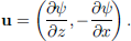
Fourier-mode solutions of Equations (68) and (69) then take the form

where substituting ψ in Equation (68) yields a quartic for m 4 + 2κm 3 + (κ 2 − 2k 2)m 2 − 2κk 2 m + k 2(κ 2 + k 2) = 0 , which has four distinct roots m 1, m 2, m 3 and m 4 when κ = 0 (in fact, these roots form complex conjugate pairs). A general Fourier-mode solution
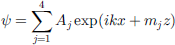
is substituted in the boundary conditions (70–73); the solution of the set of linear algebraic equations in the Aj which results is used to calculate the F and G functions by substituting in Equations (74) and (49).



