2. Laplace invariants and Laplace series

In this section, we review the main notions and facts concerning the Laplace invariants, the Laplace transformations and the Laplace series in the continuous case that we need to prove discrete analogues of the Darboux formulae. All propositions, theorems and statements of this section are known to experts in the area. Detailed proofs can be found in the original book by Darboux [Reference Darboux1], which is in French, or in the classical book [Reference Forsyth21]. The cascade method had also been discussed in a well-known book [Reference Tricomi22] in a bit of an old-fashioned way and in papers [Reference Zhiber and Sokolov23–Reference Habibullin, Faizulina and Khakimova25] from a modern perspective. Laplace invariants for differential operators of a more general form had been studied in [Reference Kamran and Tenenblat26–Reference Athorne29].

Consider the linear hyperbolic differential operator

(2.1) \begin{equation} {\mathcal L}=\partial _x\partial _y+a\partial _x+b\partial _y+c, \end{equation}

where $a$ , $b$ and $c$ are functions of the variables $x$ and $y$ . The functions $k=c-ab-a_x$ and $h=c-ab-b_y$ are called the Laplace invariants of (2.1). They are invariant under gauge transformations ${\mathcal L}\mapsto \bar {\mathcal L}=\omega ^{-1}{\mathcal L}\omega$ , where $\omega =\omega (x,y)$ is an arbitrary function and control factorisability of such an operator: since

\begin{equation*} {\mathcal L}=(\partial _x+b)(\partial _y+a)+k=(\partial _y+a)(\partial _x+b)+h, \end{equation*}

the operator $\mathcal L$ is factorisable if and only if at least one of its Laplace invariants is zero. Straightforward calculation shows that if $h=0$ , then the general solution of ${\mathcal L}\psi =0$ has the form

(2.2) \begin{equation} \psi (x,y)=\left (\int \left (X(x) e^{\int b(x,y)dx-\int a(x,y)dy}\right )dx+Y(y)\right )e^{-\int b(x,y)dx} \end{equation}

and if $k=0$ , then the general solution has the form

(2.3) \begin{equation} \psi (x,y)=\left (\int \left (Y(y) e^{\int a(x,y)dy-\int b(x,y)dx}\right )dy+X(x)\right )e^{-\int a(x,y)dy}, \end{equation}

where $X$ and $Y$ are arbitrary functions of one variable.

Two linear hyperbolic differential operators

\begin{equation*} {\mathcal L}=\partial _x\partial _y+a\partial _x+b\partial _y+c\quad \hbox{and}\quad \hat {\mathcal L}=\partial _x\partial _y+\hat a\partial _x+\hat b\partial _y+\hat c \end{equation*}

are related by a Darboux–Laplace transformation if there exist first-order operators ${\mathcal D}=\alpha \partial _x+\beta \partial _y+\gamma$ and $\hat {\mathcal D}=\hat \alpha \partial _x+\hat \beta \partial _y+\hat \gamma$ such that the following relation is satisfied:

(2.4) \begin{equation} \hat {\mathcal L}\circ {\mathcal D}=\hat {\mathcal D}\circ {\mathcal L}. \end{equation}

Two particular cases ${\mathcal D}=\partial _x+b$ and ${\mathcal D}=\partial _y+a$ correspond to classical Laplace transformations, which were widely used by Darboux and Goursat in their research on the theory of surfaces.Footnote ¹ In both cases, the coefficients of operators $\hat {\mathcal L}$ and $\hat {\mathcal D}$ are uniquely defined in terms of the coefficients of $\mathcal L$ . The main property of Darboux-Laplace transformations is that the transformation operator $\mathcal D$ maps the kernel of the operator $\mathcal L$ into the kernel of $\hat {\mathcal L}$ : if $\psi \in {\mathop {\textrm {Ker}}\nolimits }{\mathcal L}$ , then relation (2.4) implies that ${\mathcal D}\psi \in {\mathop {\textrm {Ker}}\nolimits }\hat {\mathcal L}$ . There exists a wide class of Darboux–Laplace transformations for linear hyperbolic operators different from the classical Laplace transformations (see [Reference Shemyakova30, Reference Shemyakova31]), but we will consider only classical ones throughout this paper.

Operator relation (2.4) is equivalent to a system of PDEs for the coefficients of all four operators. Proof of Proposition 1 is based on the fact that operators $\hat {\mathcal L}$ , $\mathcal L$ and $-h^{-1}(\partial _y+a)$ provide a solution to this system for the suitably chosen fourth operator.

Consider a hyperbolic operator

\begin{equation*} {\mathcal L}_0=\partial _x\partial _y+a_0\partial _x+b_0\partial _y+c_0 \end{equation*}

and apply the Laplace transformation ${\mathcal D_0}=\partial _x+b_0$ :

\begin{equation*} {\mathcal L}_1{\mathcal D}_0={\mathcal D}_1{\mathcal L}_0\quad \hbox{where}\quad {\mathcal L}_1=\partial _x\partial _y+a_1\partial _x+b_1\partial _y+c_1. \end{equation*}

Apply the Laplace transformation ${\mathcal D_1}=\partial _x+b_1$ to the operator ${\mathcal L}_1$ , etc. This procedure produces the sequence of hyperbolic operators starting from ${\mathcal L}_0$ and such that any two neighbouring operators are related by a Laplace transformation. The second Laplace transformation ${\mathcal D}'_0=\partial _y+a_0$ allows to continue the sequence to the left:

\begin{equation*} {\mathcal L}_{-1}{\mathcal D}'_0={\mathcal D}'_1{\mathcal L}_0, \end{equation*}

etc. This leads to the sequence

(2.5) \begin{equation} \ldots \stackrel {{\mathcal D}'_j}{\longleftarrow }{\mathcal L}_{-j}\stackrel {{\mathcal D}'_{j-1}}{\longleftarrow }{\mathcal L}_{-j+1}\stackrel {{\mathcal D}'_{j-2}} {\longleftarrow }\ldots \stackrel {{\mathcal D}'_1}{\longleftarrow }{\mathcal L}_{-1}\stackrel {{\mathcal D}'_0}{\longleftarrow }{\mathcal L}_0\stackrel {{\mathcal D}_0} {\longrightarrow }{\mathcal L}_1\stackrel {{\mathcal D}_1}{\longrightarrow }\ldots \stackrel {{\mathcal D}_{j-1}}{\longrightarrow }{\mathcal L}_j\stackrel {{\mathcal D}_j} {\longrightarrow }{\mathcal L}_{j+1}\stackrel {{\mathcal D}_{j+1}}{\longrightarrow }\ldots , \end{equation}

which is called the Laplace series of the operator ${\mathcal L}_0$ . If some operator ${\mathcal L}_r$ in its positive part has zero $h$ -invariant, then the sequence terminates at ${\mathcal L}_r$ since this operator is factorisable. Similarly, if ${\mathcal L}_{-s}$ has zero $k$ -invariant for some $s\geqslant 0$ , then sequence (2.5) terminates from the left. The Laplace series is said to be finite if it terminates from both sides.

Laplace invariants of any three consecutive operators in the Laplace series satisfy the relations

\begin{equation*} k_{j+1}=h_j,\quad h_{j+1}=2h_j-h_{j-1}+(\ln h_j)_{xy}. \end{equation*}

The second of these relations is one of the forms of the two-dimensional Toda lattice.

The theorem below generalises formulae (2.2) (2.3). It follows from the fact that each operator in the Laplace series is obtained from the previous one by a Laplace transformation, which maps the kernel of the initial operator into the kernel of the next one.

Theorem 1. If the Laplace series of ${\mathcal L}_0$ terminates in the term ${\mathcal L}_r$ for some $r\in \mathbb N$ , then the general solution of the equation ${\mathcal L}_0\psi =0$ is given by

(2.6) \begin{equation} \psi _0(x,y)=-\frac {1}{h_0}(\partial _y+a_0)\left (-\frac {1}{h_1}(\partial _y+a_1)\left (\ldots \left (-\frac {1}{h_{r-1}}(\partial _y+a_{r-1})\right )\ldots \right )\right )\psi _r(x,y), \end{equation}

where $\psi _r$ has the form

(2.7) \begin{equation} \psi _r(x,y)=\left (\int \left (X(x) e^{\int b_r(x,y)dx-\int a_r(x,y)dy}\right )dx+Y(y)\right )e^{-\int b_r(x,y)dx} \end{equation}

and $X$ and $Y$ are arbitrary functions of one variable. If the Laplace series of ${\mathcal L}_0$ terminates in the term ${\mathcal L}_{-s}$ for some $s\in \mathbb N$ , then the general solution is given by

(2.8) \begin{equation} \psi _0(x,y)=-\frac {1}{k_0}(\partial _x+b_0)\left (-\frac {1}{k_{-1}}(\partial _x+b_{-1})\left (\ldots \left (-\frac {1}{k_{-s+1}}(\partial _x+b_{-s+1})\right )\ldots \right )\right )\psi _{-s}(x,y), \end{equation}

where $\psi _{-s}$ is defined as follows:

\begin{equation*} \psi _{-s}(x,y)=\left (\int \left (Y(y) e^{\int a_{-s}(x,y)dy-\int b_{-s}(x,y)dx}\right )dy+X(x)\right )e^{-\int a_{-s}(x,y)dy}. \end{equation*}

Remark 2. We define Laplace transformations in an algebraic way as mappings between hyperbolic operators. Originally, Darboux introduced such transformations in geometrical terms in his study of line congruences; see [Reference Darboux1]. Within the frame of this approach, any conjugate net (i.e., a parameterised two-dimensional surface ${\mathbf r}(u,v)$ in three-dimensional Euclidean space such that the families of coordinate lines are conjugate to each other) admits two different transformations defined in the following way. Fix a coordinate line $u=\mathop {\textrm {const}}\nolimits$ and consider all coordinate lines of the other family that intersect it. They are known to form a developable surface. Edges of regression of such developable surfaces corresponding to different coordinate lines $u=\mathop {\textrm {const}}\nolimits$ form a new surface, which appears to be the Laplace image of the initial one. The second transformation is defined in a similar way using the other family of coordinate lines. This construction is described in detail also in [Reference Eizenhart32], but in a rather archaic way, or very briefly in [Reference Doliwa8]. We will not use the geometrical nature of the Laplace transformations; we only highlight their significance in classical differential geometry. Note also that the mixed derivative ${\mathbf r}(u,v)_{uv}$ is orthogonal to the normal vector to the surface for any conjugate net ${\mathbf r}(u,v)$ . Hence the relation

\begin{equation*} {\mathbf r}_{uv}+a{\mathbf r}_u+b{\mathbf r}_v=0 \end{equation*}

holds for some scalar functions $a=a(u,v)$ and $b=b(u,v)$ . Therefore, the components of the vector ${\mathbf r}(u,v)$ that parameterises the surface satisfy a linear hyperbolic equation. In a projective setting, it takes the form

\begin{equation*} {\mathbf r}_{uv}+a{\mathbf r}_u+b{\mathbf r}_v+c{\mathbf r}=0. \end{equation*}

This relates our algebraic construction with the original geometric approach developed by Darboux.

3. Darboux formulae for general solution

Formulae (2.6) and (2.8) from the previous section allow one to obtain the general solution of a particular hyperbolic equation in explicit form given that its Laplace series is finite at least in one direction. But on the one hand, they include the integration of an arbitrary function, and on the other hand, they do not provide a suitable description of all hyperbolic equations with finite Laplace series, which would be interesting from a geometrical point of view. In this section, we review the Darboux formulae from [Reference Darboux1, Reference Forsyth21] that give the general solution in a more suitable form.

Theorem 2. If the Laplace series of a hyperbolic operator ${\mathcal L}_0$ is finite, $h_r=k_{-s}=0$ for some $r,s\geqslant 0$ , then there exist coefficients $A_i(x,y)$ and $B_j(x,y)$ such that the general solution of the equation ${\mathcal L}_0\psi =0$ is given by

(3.1) \begin{equation} \psi (x,y)=A_0 X+A_1 X'+\ldots +A_s X^{(s)}+B_0 Y+B_1 Y'+\ldots +B_r Y^{(r)}, \end{equation}

where $X(x)$ and $Y(y)$ are arbitrary functions of one variable (primes and superscripts denote derivatives).

If a hyperbolic equation ${\mathcal L}_0\psi =0$ admits a solution of the form ( 3.1 ) for some $A_i(x,y)$ and $B_j(x,y)$ , then its Laplace series is finite: $h_r=k_{-s}=0$ .

Remark 3. Not every expression of the form ( 3.1 ) defines the general solution for some hyperbolic equation with the finite Laplace series since there are restrictions on the coefficients $A_i$ , $B_j$ . Indeed, consider the simplest case of an operator with zero Laplace invariants $h_0=k_0=0$ . Hence, formula ( 3.1 ) takes the form $\psi =A X+B Y$ . Differentiate it with respect to $x$ and $y$ and substitute into the initial hyperbolic equation. Since $X$ and $Y$ are arbitrary, this yields

(3.2) \begin{equation} a_0=-(\ln A)_y,\quad b_0=-(\ln B)_x,\quad (\ln A)_{xy}=(\ln B)_{xy}. \end{equation}

The third relation shows that functions $A$ and $B$ could not be chosen at random.

A complete description of all restrictions that should be imposed on the coefficients of (3.1) is given by the Darboux determinant formula.

Theorem 3. Let ${\mathcal L}_0$ be a hyperbolic operator with the finite Laplace series, where $h_r=k_{-s}=0$ for some $r,s\geqslant 0$ . Then there exists a function $\omega =\omega (x,y)$ and functions of one variable

(3.3) \begin{equation} \xi _1 (x),\xi _2 (x),\ldots ,\xi _{r+s+1}(x),\eta _1(y),\eta _2 (y),\ldots ,\eta _{r+s+1}(y) \end{equation}

such that the general solution of ${\mathcal L}_0\psi =0$ is given by

(3.4) \begin{eqnarray} \psi (x,y)=\omega (x,y)\cdot \left | \begin{array}{c@{\quad}c@{\quad}c@{\quad}c@{\quad}c@{\quad}c@{\quad}c@{\quad}c} X & X' & \ldots & X^{(s)} & Y & Y' & \ldots & Y^{(r)}\\ \xi _1 & \xi '_1 & \ldots & \xi ^{(s)}_1 & \eta _1 & \eta '_1 & \ldots & \eta ^{(r)}_1\\ \vdots &&& \vdots & \vdots &&& \vdots \\ \xi _{r+s+1} & \xi '_{r+s+1} & \ldots & \xi ^{(s)}_{r+s+1} & \eta _{r+s+1} & \eta '_{r+s+1} & \ldots & \eta ^{(r)}_{r+s+1} \end{array} \right | \end{eqnarray}

where $X(x)$ and $Y(y)$ are arbitrary functions of one variable.

For any two families of linearly independent functions of one variable ( 3.3 ) and for any function $\omega =\omega (x,y)$ there exists a hyperbolic differential operator ${\mathcal L}_0$ with the finite Laplace series that terminates at the terms $r$ and $-s$ , such that formula ( 3.4 ) provides the general solution of ${\mathcal L}_0\psi =0$ .

Example 1. In the simplest case $h_0=k_0=0$ formula ( 3.4 ) takes the form

\begin{equation*} \psi (x,y)=\omega (x,y)\left (\eta (y)X(x)-\xi (x)Y(y)\right ). \end{equation*}

This means that for any choice of $\xi$ , $\eta$ and $\omega$ the function $\psi$ defines the general solution of the corresponding hyperbolic equation with vanishing Laplace invariants. Note that in this case $a_0=-(\ln (\omega \eta ))_y$ , $b_0=-(\ln (\omega \xi ))_x$ , and the compatibility condition from ( 3.2 ) is satisfied since $\xi$ and $\eta$ are functions of one variable. For simplicity, we may set $\omega =1$ : this gives the general solution of a gauge-equivalent hyperbolic equation with zero Laplace invariants.

Remark 5. It follows from ( 3.4 ) that if functions ( 3.3 ) are linearly independent, then $\psi (x,y)\equiv 0$ if and only if pairs

\begin{equation*} (X,Y),\ (\xi _1,\eta _1),\ldots , (\xi _{r+s+1},\eta _{r+s+1}) \end{equation*}

are linearly independent with constant coefficients (see [Reference Darboux1]). This provides a procedure to construct non-zero solutions of hyperbolic operators with finite Laplace series.

Example 2. An important particular case of conjugate nets is given by the so-called Königs nets: algebraically they are characterised by an additional constraint that the Laplace invariants of the corresponding hyperbolic operator are equal (see [Reference Bobenko and Suris3]). Any operator with equal Laplace invariants is gauge-equivalent to an operator of the form $\partial _x\partial _y+c$ , so Königs nets are defined by solutions of the Moutard equation

\begin{equation*} \psi _{xy}+c\psi =0. \end{equation*}

It follows that the Laplace series is symmetric for any Königs net. Darboux formula ( 3.4 ) provides a large stock of Königs nets with finite Laplace series: in this case one has to set $\xi _i=\eta _i$ for all $i=1,2,\ldots ,r=s$ . In particular, this allows us to obtain explicit solutions for the corresponding Moutard equation. For example, if $\xi _1=1$ , $\xi _2=x$ , $\xi _3=\frac {x^2}{2}$ , then ( 3.4 ) yields

\begin{equation*} \psi (x,y)=X'+Y'+\frac {1}{x-y}(X-Y), \end{equation*}

where we choose $\omega =\frac {2}{(x-y)^2}$ for simplicity. Hence we obtain the general solution for Moutard equation

\begin{equation*} \psi _{xy}-\frac {2}{(x-y)^2}\psi =0 \end{equation*}

and, therefore, a family of Königs nets with the Laplace series of the length $3$ . Arbitrary choice of independent functions $\xi _1,\xi _2,\xi _3$ provides the general solution for some Moutard equation with the Laplace series of the length $3$ (see [Reference Darboux1]).

4. Laplace invariants in discrete case

In this section, we aggregate basic facts on the Laplace invariants, Laplace transformations and the cascade method both in the purely discrete and in the semi-discrete cases. Although, to the best of our knowledge, some of the propositions below are not contained in the existing literature in explicit form, their proofs are either trivial or similar to the proofs of analogous propositions in the continuous case. Therefore, we give only statements without proofs in this section.

In the purely discrete case, consider a sequence of hyperbolic difference operators

\begin{equation*} {\mathcal L}_j=T_n T_m+a_j T_n+b_j T_m+c_j, \end{equation*}

where functions $a_j$ , $b_j$ and $c_j$ are defined on the $(n,m)$ -lattice and $T_n$ , $T_m$ are the shift operators:

\begin{equation*} T_n\psi _{n,m}=\psi _{n+1,m}\quad T_m\psi _{n,m}=\psi _{n,m+1}. \end{equation*}

Clearly, the operator ${\mathcal L}_j$ can be factorised in two different ways:

\begin{align*} {\mathcal L}_j=&(T_n+b_{j,n,m})(T_m+a_{j,n-1,m})+a_{j,n-1,m}b_{j,n,m}k_{j,n,m}=\\ &\qquad\qquad\qquad=(T_m+a_{j,n,m})(T_n+b_{j,n,m-1})+a_{j,n,m}b_{j,n,m-1}h_{j,n,m}, \end{align*}

where

\begin{equation*} k_{j,n,m}=\frac {c_{j,n,m}}{a_{j,n-1,m}b_{j,n,m}}-1\quad \hbox{and}\quad h_{j,n,m}=\frac {c_{j,n,m}}{a_{j,n,m}b_{j,n,m-1}}-1 \end{equation*}

are the Laplace invariants of difference operators ${\mathcal L}_j$ .

In the entirely discrete case, Darboux–Laplace transformations are introduced similarly to the continuous case: difference operator $\mathcal D$ defines a transformation for a difference hyperbolic operator $\mathcal L$ if there exist a hyperbolic operator $\hat {\mathcal L}$ and operator $\hat {\mathcal D}$ such that operator relation (2.4) is satisfied. In this case, such a relation is equivalent to a system of partial difference equations on the coefficients of the operators. Even if $\mathcal D$ and $\hat {\mathcal D}$ are first-order operators, a complete description of all possible Darboux–Laplace transformations for a given difference hyperbolic operator $\mathcal L$ is still an open problem (see [Reference Smirnov33]). Nevertheless, this system of difference equations admits two simple particular solutions for any $\mathcal L$ : corresponding transformations are given by operators $T_n+b_{j,n,m-1}$ and $T_m+a_{j,n-1,m}$ . These transformations are discrete analogues of classical Laplace transformations, and we will call them discrete Laplace transformations.

Suppose any two neighbouring operators ${\mathcal L}_j$ and ${\mathcal L}_{j+1}$ are related by the Laplace transformation defined by ${\mathcal D}_j=T_n+b_{j,n,m-1}$ . Then the Laplace invariants satisfy the purely discrete two-dimensional Toda lattice [Reference Adler and Startsev6]:

\begin{equation*} k_{j+1,n,m}=h_{j,n,m},\quad \frac {h_{j,n+1,m}h_{j,n,m-1}}{h_{j,n,m}h_{j,n+1,m-1}}=\frac {(1+h_{j+1,n,m})(1+h_{j-1,n+1,m-1})}{(1+h_{j,n,m})(1+h_{j,n+1,m-1})}. \end{equation*}

Discrete Darboux–Laplace transformations of a more general form were considered in [Reference Smirnov33].

Remark 7. Note that in the discrete case the Laplace invariants are defined not quite similarly to the continuous case: there is division by $a_{j,n,m}$ and by $b_{j,n,m}$ . This comes from the fact that functions

\begin{equation*} \tilde k_{j,n,m}=c_{j,n,m}-a_{j,n-1,m}b_{j,n,m},\quad \tilde h_{j,n,m}=c_{j,n,m}-a_{j,n,m}b_{j,n,m-1} \end{equation*}

are not invariant with respect to gauge transformations.

In the continuous case, we can use the cascade method for finding the general solution of a hyperbolic equation whenever its Laplace series terminates. But in order to do this, we need to find the general solution of the corresponding hyperbolic equation with zero Laplace invariant. In the discrete case, there is a problem that the apparatus of difference equations is less developed than the apparatus of differential equations: it is possible to express the general solution of a factorisable hyperbolic differential equation in compact form (2.2) or (2.3) using integration, although appropriate notation for a similar situation in the discrete case does not exist in mathematics. Indeed, using the representation

\begin{equation*} {\mathcal L}=(T_n+b_{n,m})(T_m+a_{n-1,m}) \end{equation*}

of a difference operator for which $k_{n,m}=0$ , one can denote ${\varphi }_{n,m}=\psi _{n,m+1}+a_{n-1,m}\psi _{n,m}$ and consider non-homogeneous difference equation ${\varphi }_{n+1,m}+b_{n,m}{\varphi }_{n,m}=0$ for the new unknown function ${\varphi }_{n,m}$ . For any integers $n,m$ the value of ${\varphi }_{n,m}$ can be recursively expressed in terms of the coefficients and the initial data ${\varphi }_{0,m}$ . Consecutively, given ${\varphi }_{n,m}$ , one can solve the first order difference equation for $\psi _{n,m+1}$ and write down the general solution in terms of the initial data $\psi _{k,0}$ and $\psi _{0,k}$ . For example, for positive values of $m$ this expression has the form

(4.1) \begin{equation} \psi _{n,m}=\alpha _{n,m}\psi _{n,0}+\gamma ^0_{n,m}\psi _{0,0}+\gamma ^1_{n,m}\psi _{0,1}+\gamma ^2_{n,m}\psi _{0,2}+\ldots +\gamma ^m_{n,m}\psi _{0,m}, \end{equation}

where $\alpha$ , $\gamma ^k$ are some coefficients. Unfortunately, the particular form of this expression is rather ugly and depends on the signs of integers $n$ and $m$ . Therefore, we do not make an attempt to give this formula explicitly and only emphasise that there exists an effective way to express the general solution in terms of the initial data $N_n=\psi _{n,0}$ and $M_m=\psi _{0,m}$ once the corresponding difference operator is factorisable. Note that expression (4.1) is local in arbitrary function $N_n$ and non-local in arbitrary function $M_m$ (i.e., it depends on a variable number of its shifts). Similarly, if $h_{n,m}=0$ , then the general solution can be expressed in the form

(4.2) \begin{equation} \psi _{n,m}=\beta _{n,m}\psi _{0,m}+\delta ^0_{n,m}\psi _{0,0}+\delta ^1_{n,m}\psi _{1,0}+\delta ^2_{n,m}\psi _{2,0}+\ldots +\delta ^n_{n,m}\psi _{n,0}. \end{equation}

Another way to represent the general solution of a hyperbolic difference equation with a factorisable operator is given by

Theorem 4. If the Laplace series of ${\mathcal L}_0$ terminates in the term ${\mathcal L}_r$ for some $r\in \mathbb N$ , then the general solution of the equation ${\mathcal L}_0\psi =0$ is given by

(4.3) \begin{align} \psi _{0,n,m}=-\frac {1}{a_{0,n,m}b_{0,n-1,m}h_{0,n,m}}(T_m+a_{0,n,m})\left (-\frac {1}{a_{1,n,m}b_{1,n-1,m}h_{1,n,m}}(T_m+a_{1,n,m})\ldots \right .\nonumber \\ \ldots \left .\left (-\frac {1}{a_{r-1,n,m}b_{r-1,n-1,m}h_{r-1,n,m}}(T_m+a_{r-1,n,m})\right )\ldots \right )\psi _{r,n,m}, \end{align}

where $\psi _r$ is the general solution of a factorisable equation ${\mathcal L}_r\psi =0$ .

If the Laplace series of ${\mathcal L}_0$ terminates in the term ${\mathcal L}_{-s}$ for some $s\in \mathbb N$ , then the general solution is given by

\begin{align*} \psi _{0,n,m}=-\frac {1}{a_{0,n,m-1}b_{0,n,m}h_{0,n,m}}(T_n+b_{0,n,m})\left (-\frac {1}{a_{-1,n,m-1}b_{-1,n,m}h_{-1,n,m}}(T_n+b_{1,n,m})\ldots \right .\\ \ldots \left .\left (-\frac {1}{a_{-s+1,n,m-1}b_{-s+1,n,m}h_{-s+1,n,m}}(T_n+b_{-s+1,n,m})\right )\ldots \right )\psi _{-s,n,m}, \end{align*}

where $\psi _{-s}$ is the general solution of a factorisable equation ${\mathcal L}_{-s}\psi =0$ .

Consider a sequence of hyperbolic differential-difference operators

(4.4) \begin{equation} {\mathcal L}_j=\partial _x T_n+a_{j,n}\partial _x+b_{j,n} T_n+c_{j,n}, \end{equation}

where $a_{j,n}$ , $b_{j,n}$ and $c_{j,n}$ are functions depending on discrete variable $n\in \mathbb Z$ and on continuous variable $x\in \mathbb R$ and where $T$ is the shift operator: $T_n\psi _n (x)=\psi _{n+1}(x)$ . The operator ${\mathcal L}_j$ can be rewritten in two different ways,

\begin{equation*} {\mathcal L}_j=(\partial _x+b_{j,n})(T+a_{j,n})+a_{j,n}k_{j,n}=(T+a_{j,n})(\partial _x+b_{j,n-1})+a_{j,n}h_{j,n}, \end{equation*}

where

\begin{equation*} k_{j,n}=\frac {c_{j,n}}{a_{j,n}}-(\ln a_{j,n})'_x-b_{j,n}\quad \hbox{and}\quad h_{j,n}=\frac {c_{j,n}}{a_{j,n}}-b_{j,n-1} \end{equation*}

are the Laplace invariants of differential-difference operator ${\mathcal L}_j$ . Similarly to the continuous case operator (4.4) can be factorised if and only if at least one of its Laplace invariants vanishes.

Suppose any two neighbouring operators ${\mathcal L}_j$ and ${\mathcal L}_{j+1}$ are related by a Laplace transformation, that is, they satisfy relation (2.4), where ${\mathcal D}_j=\partial _x+b_{j,n-1}$ . This operator relation can be rewritten in terms of coefficients:

\begin{eqnarray*} \left \lbrace \begin{array}{l} k_{j+1,n}=h_{j,n}\\ \left (\ln \frac {h_{j,n}}{h_{j,n+1}}\right )'_x=h_{j+1,n+1}-h_{j,n+1}-h_{j,n}+h_{j-1,n} \end{array} \right .. \end{eqnarray*}

These equations are one of the forms of the semi-discrete two-dimensional Toda lattice [Reference Adler and Startsev6]. Laplace transformations in the variable $n$ are defined by difference operators ${\mathcal D}'_j=T_n+a_{j,n}$ .

Remark 10. In the semi-discrete case, the division by $a_{j,n}$ in the definition of the Laplace invariants is also necessary because the functions

\begin{equation*} \tilde k_{j,n}=c_{j,n}-a_{j,n,x}-a_{j,n}b_{j,n},\quad \tilde h_{j,n}=c_{j,n}-a_{j,n}b_{j,n-1} \end{equation*}

are not invariant with respect to gauge transformations of the form ${\mathcal L}\to \omega ^{-1}_{n+1}{\mathcal L}\omega _n$ . Therefore, in this case, we also assume that the coefficients $a_{0,n}$ are non-zero. Since operator relation ( 2.4 ) yields the condition $a_{j,n}=a_{j+1,n}$ , the coefficients of all operators in the lattice do not turn into zero, and hence, the Laplace invariants are well-defined.

Similarly to the continuous case, the following proposition holds.

5. Darboux formulae in discrete case

In this section, we prove the analogues of the Darboux formulae for the general solution of a linear hyperbolic equation with the finite Laplace series in a purely discrete case. Our aim is to prove the following:

Theorem 5. Let ${\mathcal L}_0$ be a hyperbolic difference operator with a finite Laplace series where $h_r=k_{-s}=0$ for some $r,s\geqslant 0$ . Then there exist functions

(5.1) \begin{equation} \nu _{1,n},\nu _{2,n},\ldots ,\nu _{r+s+1,n}\quad \hbox{and}\quad \mu _{1,m},\mu _{2,m},\ldots ,\mu _{r+s+1,m} \end{equation}

of one discrete variable and a function $\omega _{nm}$ such that the general solution of ${\mathcal L}_0\psi =0$ is given by the determinant formula

(5.2) \begin{align} \psi _{0,n,m}=\nonumber \\& =\omega _{n,m}\cdot \det \left (\begin{array}{c@{\quad}c@{\quad}c@{\quad}c@{\quad}c@{\quad}c@{\quad}c@{\quad}c} M_m & M_{m+1} & \ldots & M_{m+r} & N_n & N_{n+1} & \ldots & N_{n+s}\\ \mu _{1,m} & \mu _{1,m+1} & \ldots & \mu _{1,m+r} & \nu _{1,n} & \nu _{1,n+1} & \ldots & \nu _{1,n+s}\\ \mu _{2,m} & \mu _{2,m+1} & \ldots & \mu _{2,m+r} & \nu _{2,n} & \nu _{2,n+1} & \ldots & \nu _{2,n+s}\\ \vdots &&&\vdots &&&&\vdots \\ \mu _{r+s+1,m} & \mu _{r+s+1,m+1} & \ldots & \mu _{r+s+1,m+r} & \nu _{r+s+1,n} & \nu _{r+s+1,n+1} & \ldots & \nu _{r+s+1,n+s} \end{array} \right ), \end{align}

where $N_n$ and $M_m$ are arbitrary functions of one variable.

For any two families of linearly independent functions of one variable ( 5.1 ) and for any function $\omega _{n,m}$ there exists a hyperbolic difference operator ${\mathcal L}_0$ with a finite Laplace series that terminates at the terms $r$ and $-s$ such that formula ( 5.2 ) provides the general solution of ${\mathcal L}_0\psi =0$ .

The proof of this general result is divided into a number of propositions, lemmas and theorems.

Lemma 1. If the Laplace series of ${\mathcal L}_0$ terminates at the term ${\mathcal L}_r$ where $r\gt 0$ , then the equation ${\mathcal L}_0\psi =0$ admits a solution of the form

(5.3) \begin{equation} \psi _{0,n,m}=B_{0,n,m} M_m+B_{1,n,m} M_{m+1}+\cdots +B_{r,n,m} M_{m+r}, \end{equation}

where $M_m$ is an arbitrary function of one discrete variable. If the Laplace series terminates at the term ${\mathcal L}_{-s}$ where $s\gt 0$ , then the equation ${\mathcal L}_0\psi =0$ admits a solution of the form

(5.4) \begin{equation} \psi _{0,n,m}=A_{0,n,m} N_n+A_{1,n,m} N_{n+1}+\cdots +A_{s,n,m} N_{n+s}, \end{equation}

where $N_n$ is an arbitrary function of one discrete variable.

Proof. Use induction in $r$ to prove the first claim. If $r=0$ , then the equation ${\mathcal L}_0\psi =0$ admits a solution of the form $\psi _{n,m}=B_{0,n,m} M_m$ . Substitute it into the equation:

\begin{equation*} B_{0,n+1,m+1} M_{m+1}+a_{n,m} B_{0,n+1,m} M_m+b_{n,m} B_{0,n,m+1} M_{m+1}+c_{n,m}B_{0,n,m} M_m=0. \end{equation*}

Since $M$ is arbitrary, this leads to equations

\begin{eqnarray*} \left \{ \begin{array}{l} B_{0,n+1,m+1}+b_{n,m} B_{0,n,m+1}=0\\ a_{n,m} B_{0,n+1,m}+c_{n,m}B_{0,n,m}=0 \end{array} \right .. \end{eqnarray*}

Multiply the first equation by $a_{n,m+1}$ , shift the second equation in $m$ and consider the difference:

\begin{equation*} a_{n,m+1}b_{n,m} B_{0,n,m+1}-c_{n,m+1}B_{0,n,m+1}=0 \end{equation*}

This relation has to be satisfied for all natural $n,m$ . Hence $a_{n,m+1}b_{n,m}-c_{n,m+1}=0$ , which is equivalent to $h_{n,m+1}=0$ .

Assume the proposition holds for all equations admitting solutions (5.3) of order $r$ . Consider equation ${\mathcal L}_0\psi =0$ having such a solution of order $r+1$ . This means that the result of substitution of this solution into the equation, which is an expression of the form

(5.5) \begin{equation} C_{0,n,m}M_m+C_{1,n,m}M_{m+1}+\cdots +C_{r+2,n,m}M_{m+r+2}, \end{equation}

identically vanishes. Note that the leading coefficient in (5.5) has the form

(5.6) \begin{equation} C_{r+2,n,m}=B_{r+1,n+1,m+1}+b_{n,m}B_{r+1,n,m+1}=0. \end{equation}

If $h_0=0$ , then the proposition is proved. Otherwise, apply the Laplace transformation $T_n+b_{n,m-1}$ :

\begin{align*} \psi _{1,n,m}=(T_n+b_{n,m-1})\left (B_{0,n,m} M_m+B_{1,n,m} M_{m+1}+\cdots +B_{r+1,n,m} M_{m+r+1}\right )=\\ =b_{n,m-1}B_{0,n,m} M_m+\cdots +(B_{r+1,n+1,m}+b_{n,m-1}B_{r+1,n,m}) M_{m+r+1} \end{align*}

Compare the leading coefficient in the latter expression with (5.6) to conclude that $\psi _1$ has the form (5.3) of order $r$ and hence by the assumption the Laplace series of the corresponding operator ${\mathcal L}_1$ terminates at the term ${\mathcal L}_p$ , where $p\leqslant r$ . But ${\mathcal L}_1$ is the next term in the Laplace series of the initial operator ${\mathcal L}_0$ . Therefore, its Laplace series terminates not later than at the $(r+1)$ -th term. The second claim is proved similarly.

Lemma 3. If the Laplace invariants of ${\mathcal L}_0$ are non-zero and the general solution of the hyperbolic equation ${\mathcal L}_0\psi =0$ has the form

(5.7) \begin{equation} \psi _{0,n,m}=A_{0,n,m} N_n+A_{1,n,m} N_{n+1}+\cdots +A_{s,n,m} N_{n+s}+B_{0,n,m} M_m+B_{1,n,m} M_{m+1}+\cdots +B_{r,n,m} M_{m+r}, \end{equation}

where $M$ and $N$ are arbitrary functions of one discrete variable and $A_0\ne 0$ , $A_s\ne 0$ , $B_0\ne 0$ , $B_r\ne 0$ , then the general solution of the equation ${\mathcal L}_1\psi =0$ , where ${\mathcal L}_1=(T_n+b_{n,m-1}){\mathcal L}_0$ , has the form

\begin{equation*} \psi _{1,n,m}=\hat A_{0,n,m} N_n+\hat A_{1,n,m} N_{n+1}+\cdots +\hat A_{s+1,n,m} N_{n+s+1}+\hat B_{0,n,m} M_m+\hat B_{1,n,m} M_{m+1}+\cdots + \hat B_{r-1,n,m} M_{m+r-1}, \end{equation*}

where $\hat A_0\ne 0$ , $\hat A_{s+1}\ne 0$ , $\hat B_0\ne 0$ , $\hat B_{r-1}\ne 0$ , and the general solution of the equation ${\mathcal L}_{-1}\psi =0$ , where ${\mathcal L}_{-1}=(T_m+a_{n-1,m}){\mathcal L}_0$ , has the form

\begin{equation*} \psi _{-1,n,m}=\tilde A_{0,n,m} N_n+\tilde A_{1,n,m} N_{n+1}+\cdots +\tilde A_{s-1,n,m} N_{n+s-1}+\tilde B_{0,n,m} M_m+\tilde B_{1,n,m} M_{m+1}+ \cdots +\tilde B_{r+1,n,m} M_{m+r+1}, \end{equation*}

where $\tilde A_0\ne 0$ , $\tilde A_{s-1}\ne 0$ , $\tilde B_0\ne 0$ , $\tilde B_{r+1}\ne 0$ .

Proof. Apply the Laplace transformation to (5.7) to get the general solution of ${\mathcal L}_1\psi =0$ . Obviously it has the form

\begin{equation*} \psi _{1,n,m}=\hat A_{0,n,m} N_n+\hat A_{1,n,m} N_{n+1}+\cdots +\hat A_{s+1,n,m} N_{n+s+1}+\hat B_{0,n,m} M_m+\hat B_{1,n,m} M_{m+1}+\cdots + \hat B_{r,n,m} M_{m+r}, \end{equation*}

and we need to prove that $\hat B_{r,n,m}=0$ . Note that

(5.8) \begin{equation} \hat A_{s+1,n,m}=A_{s,n+1,m},\quad \hat B_{r,n,m}=B_{r,n+1,m}+b_{n,m-1} B_{r,n,m},\quad \hat B_{r-1,n,m}=B_{r-1,n+1,m}+b_{n,m-1} B_{r-1,n,m}; \end{equation}

hence, $\hat A_{s+1}\ne 0$ . Substitute (5.7) into hyperbolic equation ${\mathcal L}_0\psi =0$ . This gives an expression of the form

\begin{equation*} C_{0,n,m} N_n+C_{1,n,m} N_{n+1}+\cdots +C_{s+1,n,m} N_{n+s+1}+ D_{0,n,m} M_m+D_{1,n,m} M_{m+1}+\cdots +D_{r+1,n,m} M_{m+r+1}=0. \end{equation*}

Since functions $M$ and $N$ are arbitrary, all coefficients vanish. In particular,

\begin{equation*} 0=D_{r+1,n,m}=B_{r,n+1,m+1}+b_{n,m}B_{r,n,m+1}. \end{equation*}

Compare this with the second relation in (5.8) to verify that $\hat B_r=0$ . Besides this,

(5.9) \begin{equation} 0=D_{r,n,m}=B_{r-1,n+1,m+1}+a_{n,m}B_{r,n+1,m}+b_{n,m}B_{r-1,n,m+1}+c_{n,m}B_{r,n,m}. \end{equation}

Assume that $\hat B_{r-1}=0$ . Hence (5.8) yields $B_{r-1,n+1,m+1}=-b_{n,m} B_{r-1,n,m+1}$ . Therefore, (5.9) can be rewritten as

\begin{equation*} 0=\left (c_{n,m}-a_{n,m}b_{n,m-1}\right )B_{r,n,m}=a_{n,m}b_{n,m-1}h_{n,m}B_{r,n,m}, \end{equation*}

which contradicts the assumption $B_r\ne 0$ since $h$ is non-zero.

Note that

\begin{equation*} \hat A_{0,n,m}=b_{n,m-1}A_{0,n,m}\ne 0,\quad \hat B_{0,n,m}=B_{0,n+1,m}+b_{n,m-1}B_{0,n,m}. \end{equation*}

If $\hat B_{0,n,m}=0$ , then express $B_{0,n+1,m}=-b_{n,m-1}B_{0,n,m}$ and substitute this into the equation $D_{0,n,m}=0$ :

\begin{equation*} 0=a_{n,m}B_{0,n+1,m}+c_{n,m}B_{n,m}=\left (c_{n,m}-a_{n,m}b_{n,m-1}\right )B_{0,n,m}. \end{equation*}

Since $h\ne 0$ , we arrive at a contradiction. The second claim is obtained similarly.

Proof. The general solution of ${\mathcal L}_0=0$ can be obtained by the application of $s$ Laplace transformations to the general solution of ${\mathcal L}_{-s}=0$ . We will construct such a solution in a special form. Since $h_{-s}=0$ , operator ${\mathcal L}_{-s}$ can be factorised, and therefore, according to Proposition 3, the general solution has the form $\psi _{-s,n,m}=\theta _{n,m}+\theta ^0_{n,m}$ . Note that $\theta _{n,m}=\alpha _{n,m}N_n$ , where $N_n$ is an arbitrary function of one variable and $\alpha _{n,m}$ depends on coefficients of ${\mathcal L}_{-s}$ . Similarly, the general solution of the equation ${\mathcal L}_r=0$ has the form $\psi _{r,n,m}=\chi _{n,m}+\chi ^0_{n,m}$ , where $\chi _{n,m}=\beta _{n,m}M_m$ and $M_m$ is an arbitrary function. Set $\chi ^0=0$ and apply the composition $\mathcal M$ of inverse Laplace transformations:

\begin{equation*} {\mathcal M}\chi _{n,m}=\omega _{n,m}\left (T_m+a_{-s+1,n-1,m}\left )\right (T_m+a_{-s+2,n-1,m}\right )\ldots \left (T_m+a_{r,n-1,m}\right )\chi _{n,m}\in {\mathop {\textrm {Ker}}\nolimits }{\mathcal L}_{-s} \end{equation*}

(see Remark 9). Since $\chi _{n,m}=\beta _{n,m}M_m$ depends on an arbitrary function and

\begin{equation*} \left (T_n+b_{-s,n,m}\right )\left (T_m+a_{-s,n-1,m}\right ){\mathcal M}\chi _{n,m}=0, \end{equation*}

the function ${\varphi }_{n,m}=\left (T_m+a_{-s,n-1,m}\right ){\mathcal M}\chi _{n,m}$ parameterises the general solution of the homogeneous equation $\left (T_n+b_{-s,n,m}\right )\psi _{n,m}=0$ . Hence, $\theta ^0_{n,m}={\mathcal M}\chi _{n,m}$ satisfies the non-homogeneous equation

\begin{equation*} \left (T_m+a_{-s,n-1,m}\right )\psi _{n,m}={\varphi }_{n,m}. \end{equation*}

Therefore the general solution of ${\mathcal L}_{-s}\psi =0$ has the form

\begin{equation*} \psi _{-s,n,m}=\alpha _{n,m}N_n+{\mathcal M}\chi _{n,m}. \end{equation*}

Apply the Laplace transformations ${\mathcal N}=\left (T_n+b_{-1,n,m-1}\right )\ldots \left (T_n+b_{-s,n,m-1}\right )$ to obtain the general solution of ${\mathcal L}_0\psi =0$ :

\begin{align*} \psi _{0,n,m}={\mathcal N}\left (\alpha _{n,m}N_n+{\mathcal M}\chi _{n,m}\right )= {\mathcal N}\left (\alpha _{n,m}N_n\right )+\tilde \omega _{n,m}\left (T_m+a_{1,n-1,m}\right )\ldots \left (T_m+a_{r,n-1,m}\right )\left (\beta _{n,m}M_m\right )=\\ =A_{0,n,m} N_n+A_{1,n,m} N_{n+1}+\cdots +A_{s,n,m} N_{n+s}+B_{0,n,m} M_m+B_{1,n,m} M_{m+1}+\cdots +B_{r,n,m} M_{m+r} \end{align*}

since $\mathcal N$ and $\left (T_m+a_{1,n-1,m}\right )\ldots \left (T_m+a_{r,n-1,m}\right )$ are difference operators in $T_n$ and $T_m$ of orders $s$ and $r$ respectively.

The second claim follows from Lemmas 2, 3.

Suppose the Laplace series of ${\mathcal L}_0$ is finite, $h_r=k_{-s}=0$ for some $r,s\geqslant 0$ , and the operators ${\mathcal L}_{-s+1},\ldots ,{\mathcal L}_{r-1}$ have non-zero Laplace invariants. Then the general solution of the equation ${\mathcal L}_r\psi =0$ has the form

\begin{equation*} \psi _{r,n,m}=A_{0,n,m} N_n+A_{1,n,m} N_{n+1}+\cdots +A_{r+s,n,m} N_{n+r+s}+B_{0,n,m} M_m. \end{equation*}

Without loss of generality, one may assume that $B_0=1$ (apply an appropriate gauge transformation, which does not change the Laplace invariants). Hence, the hyperbolic equation ${\mathcal L}_r\psi =0$ admits a solution of the form $\psi _{r,n,m}=M_m$ . This yields $b_{r,n,m}=-1$ , $a_{r,n,m}=-c_{r,n,m}$ . Thus,

\begin{equation*} {\mathcal L}_r=\left (T_m+a_{r,n,m}\right )\left (T_n-1\right )\quad \hbox{and}\quad \left (T_n-1\right )\psi _{r,n,m}\in {\mathop {\textrm {Ker}}\nolimits }\left (T_m+a_{r,n,m}\right ). \end{equation*}

Therefore, $\left (T_n-1\right )\psi _{r,n,m}=\alpha _{n,m}\tilde N_n$ for a certain $\tilde N$ . This leads to the relation

(5.10) \begin{align} -A_{0,n,m} N_n+(A_{0,n+1,m}-A_{1,n,m}) N_{n+1}+\cdots +\nonumber \\ +(A_{r+s-1,n+1,m}-A_{r+s,n,m}) N_{n+r+s}+A_{r+s,n+1,m} N_{n+r+s+1}=\alpha _{n,m}\tilde N_n. \end{align}

Denote

\begin{equation*} \lambda _{0,n,m}=-\frac {A_{0,n,m}}{\alpha _{n,m}},\quad \lambda _{1,n,m}=\frac {A_{0,n+1,m}-A_{1,n,m}}{\alpha _{n,m}},\ldots , \lambda _{r+s+1,n,m}=\frac {A_{r+s,n+1,m}}{\alpha _{n,m}}. \end{equation*}

Note that all coefficients $\lambda _0,\ldots ,\lambda _{r+s+1}$ do not depend on $m$ since $N_n$ and $\tilde N_n$ are functions of one discrete variable $n$ . Therefore we drop the second index in $\lambda _{0,n,m},\ldots ,\lambda _{r+s+1,n,m}$ for convenience.

Proof. Express the functions $A_{i,n,m}$ in terms of $\alpha _{n,m}$ and $\lambda _0,\ldots ,\lambda _{r+s+1}$ :

\begin{align*} A_{0,n,m}&=-\alpha _{n,m}\lambda _{0,n}\\ A_{1,n,m}&=A_{0,n+1,m}-\alpha _{n,m}\lambda _{1,n}=-T_n\left (\alpha _{n,m}\lambda _{0,n}\right )-\alpha _{n,m}\lambda _{1,n}\\ A_{2,n,m}&=A_{1,n+1,m}-\alpha _{n,m}\lambda _{2,n}=-T^2_n\left (\alpha _{n,m}\lambda _{0,n}\right )-T_n\left (\alpha _{n,m}\lambda _{1,n}\right )-\alpha _{n,m}\lambda _{2,n}\\ \ldots \\ A_{r+s,n,m}&=A_{r+s-1,n+1,m}-\alpha _{n,m}\lambda _{r+s,n}=-\sum \limits _{i=0}^{r+s}T^i_n\left (\alpha _{n,m}\lambda _{r+s-i,n}\right )\\ A_{r+s,n+1,m}&=\alpha _{n,m}\lambda _{r+s+1,n}. \end{align*}

Hence, function $\alpha _{n,m}$ satisfies the linear difference equation

(5.11) \begin{equation} \lambda _{0,n} T^{r+s+1}_n\alpha _{n,m}+\ldots +\lambda _{r+s} T_n\alpha _{n,m}+\lambda _{r+s+1}\alpha _{n,m}=0.\quad \end{equation}

Let $\nu _{1,n},\nu _{2,n},\ldots ,\nu _{r+s+1,n}$ be a fundamental system of solutions of linear ordinary difference equation (5.11). Then $\tilde N=0$ once $N=\nu _i$ is chosen in (5.10) for some $i=1,2,\ldots ,r+s+1$ . Hence

\begin{equation*} \left (T_n-1\right )\left (A_{0,n,m} \nu _{i,n}+A_{1,n,m} \nu _{i,n+1}+\cdots +A_{r+s,n,m} \nu _{i,n+r+s}+M_m\right )=0 \end{equation*}

for every $i=1,2,\ldots ,r+s+1$ . This means that

\begin{equation*} \mu _{i,m}:=A_{0,n,m} \nu _{i,n}+A_{1,n,m} \nu _{i,n+1}+\cdots +A_{r+s,n,m} \nu _{i,n+r+s},\quad i=1,2,\ldots ,r+s+1, \end{equation*}

are functions only of $m$ .

Proposition 6. In the above setting, the general solution of the equation ${\mathcal L}_r\psi =0$ is given by $\psi _r=\frac {\Delta _1}{\Delta }$ , where

(5.12) \begin{eqnarray} \Delta _{1,n,m}=\det \left ( \begin{array}{ccccc} M_m & N_n & N_{n+1} & \ldots & N_{n+r+s}\\ \mu _{1,m} & \nu _{1,n} & \nu _{1,n+1} & \ldots & \nu _{1,n+r+s}\\ \mu _{2,m} & \nu _{2,n} & \nu _{2,n+1} & \ldots & \nu _{2,n+r+s}\\ \vdots &&&\ddots &\vdots \\ \mu _{r+s+1,m} & \nu _{r+s+1,n} & \nu _{r+s+1,n+1} & \ldots & \nu _{n+s+1,n+r+s} \end{array} \right ), \end{eqnarray}

(5.13) \begin{eqnarray} \Delta _{n,m}=\det \left ( \begin{array}{cccc} \nu _{1,n} & \nu _{1,n+1} & \ldots & \nu _{1,n+r+s}\\ \nu _{2,n} & \nu _{2,n+1} & \ldots & \nu _{2,n+r+s}\\ \vdots &&\ddots &\vdots \\ \nu _{r+s+1,n} & \nu _{r+s+1,n+1} & \ldots & \nu _{n+s+1,n+r+s} \end{array} \right ). \end{eqnarray}

Proof. Let $\psi _r$ be the general solution of ${\mathcal L}_r\psi =0$ . Then there exist families of functions $\nu _1,\ldots ,\nu _{r+s+1}$ and $\mu _1,\ldots ,\mu _{r+s+1}$ depending on $n$ and $m$ respectively such that the following relations are satisfied:

(5.14) \begin{equation} \left \{ \begin{aligned} \psi _{r,n,m}&-A_{0,n,m} N_n-A_{1,n,m} N_{n+1}-\cdots -A_{r+s,n,m} N_{n+r+s}=M_m\\ &-A_{0,n,m}\nu _{i,n}-A_{1,n,m} \nu _{i,n+1}-\cdots -A_{r+s,n,m} \nu _{i,n+r+s}=\mu _{i,m},\quad i=1,2,\ldots ,r+s+1\\ \end{aligned} \right .. \end{equation}

Solve this system with respect to the unknowns $\psi _r,-A_0,-A_1,\ldots ,-A_{r+s}$ and apply Cramer’s rule to obtain the formula for $\psi _r$ .

Consider the general solution of ${\mathcal L}_0\psi =0$ . On the one hand, it has the form (5.7); on the other hand, it is obtained from the general solution of equation ${\mathcal L}_r\psi =0$ by application of Laplace transformations: $\psi _r={\mathcal M}\psi _0$ , where $\mathcal M$ is a difference operator of order $r$ and $\psi _r$ is the quotient of determinants (5.12) and (5.13). Hence $\psi _0=0$ whenever $N=\nu _i$ and $M=\mu _i$ for a certain $i=1,2,\ldots ,r+s+1$ . Therefore, up to multiplication by an appropriate function $\omega _{n,m}$ , the following equations are satisfied:

\begin{equation*} \left \{ \begin{aligned} \psi _{0,n,m}&-B_{0,n,m} M_n-\cdots -B_{r,n,m} M_{n+r}-A_{0,n,m} N_n-\cdots -A_{s,n,m} N_{n+s}=0\\ &-B_{0,n,m}\mu _{i,n}-\cdots -B_{r,n,m} \mu _{i,n+r}-A_{0,n,m}\nu _{i,n}-\cdots -A_{s,n,m} \nu _{i,n+s}=0,\quad i=1,2,\ldots ,r+s+1\\ \end{aligned} \right .. \end{equation*}

Solve this system with respect to the unknowns $\psi _0,-B_0,\ldots ,-B_r,-A_0,\ldots ,A_s$ and apply the projective version of Cramer’s rule to obtain (5.2). This proves the first part of Theorem 5.

In order to prove the second part of Theorem 5, choose arbitrary independent functions of one variable

(5.15) \begin{equation} \nu _{1,n},\nu _{2,n},\ldots ,\nu _{r+s+1,n}\quad \hbox{and}\quad \mu _{1,m},\mu _{2,m},\ldots ,\mu _{r+s+1,m} \end{equation}

and solve linear system (5.14) for $A_0,A_1,\ldots ,A_{r+s}$ . This provides

(5.16) \begin{equation} \psi _{r,n,m}=A_{0,n,m} N_n+A_{1,n,m} N_{n+1}+\cdots +A_{r+s,n,m} N_{n+r+s}+M_m. \end{equation}

Proof. Since $\mu _{i,m}=-A_{0,n,m}\nu _{i,n}-A_{1,n,m} \nu _{i,n+1}-\cdots -A_{r+s,n,m} \nu _{i,n+r+s}$ is a function of $m$ for every $\quad i=1,2,\ldots ,r+s+1$ , function $\nu _i$ satisfies the difference equation

\begin{equation*} \left (T_n-1\right )\left (A_{0,n,m} \nu _{i,n}+A_{1,n,m} \nu _{i,n+1}+\cdots +A_{r+s,n,m} \nu _{i,n+r+s}\right )=0, \end{equation*}

which has order $r+s+1$ . Consider the linear ordinary difference equation

\begin{equation*} \lambda _{0,n}\nu _{n+r+s+1}+\cdots +\lambda _{r+s,n}\nu _{n+1}+\lambda _{r+s+1,n}\nu _n=0, \end{equation*}

having $\nu _{1,n},\nu _{2,n},\ldots ,\nu _{r+s+1,n}$ as a basis in the space of solutions. Such an equation is unique up to multiplication by an arbitrary function $\alpha _{n,m}$ . Therefore, the following relations are satisfied:

\begin{equation*} \alpha _{n,m}=-\frac {A_{0,n,m}}{\lambda _{0,n,m}}=\frac {A_{0,n+1,m}-A_{1,n,m}}{\lambda _{1,n}}=\ldots = \frac {A_{r+s-1,n+1,m}-A_{r+s,n,m}}{\lambda _{r+s,n}}=\frac {A_{r+s,n+1,m}}{\lambda _{r+s+1,n}}. \end{equation*}

This implies that $\left (T_n-1\right )\psi _{r,n,m}=\alpha _{n,m}\tilde N_n$ , where $\tilde N$ is a function of $n$ . Hence

\begin{equation*} \left (T_m+\gamma _{n,m}\right )\left (T_n-1\right )\psi _{r,n,m}=\left (T_m+\gamma _{n,m}\right )\left (\alpha _{n,m}\tilde N_n\right )= \left (\alpha _{n,m+1}+\gamma _{n,m}\alpha _{n,m}\right )\tilde N_n \end{equation*}

for any $\gamma _{n,m}$ . Therefore if $\gamma _{n,m}=-\frac {\alpha _{n,m+1}}{\alpha _{n,m}}$ for all $n,m\in \mathbb Z$ , then ${\mathcal L}_r\psi _r=0$ , where

\begin{equation*} {\mathcal L}_r=\left (T_m+\gamma _{n,m}\right )\left (T_n-1\right )=T_nT_m+\gamma _{n,m}T_n-T_m-\gamma _{n,m}. \end{equation*}

Note that $h_r=0$ for any operator of such kind.

According to Theorem 6, if the hyperbolic equation ${\mathcal L}_r\psi =0$ admits a solution of the form (5.16), then the Laplace series of ${\mathcal L}_r$ is finite. In particular, $h_{-s}=0$ . Apply Laplace transformations to ${\mathcal L}_r$ and to $\psi _r$ in order to obtain the operator ${\mathcal L}_0$ in the Laplace series and the general solution of the equation ${\mathcal L}_0\psi =0$ . On the one hand it has the form

\begin{equation*} \psi _{0,n,m}=C_{0,n,m} N_n+C_{1,n,m} N_{n+1}+\ldots +C_{s,n,m} N_{n+s}+D_{0,n,m} M_m+D_{1,n,m} M_{m+1}+\ldots +D_{r,n,m} M_{m+r}. \end{equation*}

On the other hand, consider the determinant in (5.2) constructed using functions (5.15) and expand it along its first row. This expression has the form

\begin{equation*} \tilde \psi _{0,n,m}=\tilde A_{0,n,m} N_n+\tilde A_{1,n,m} N_{n+1}+\cdots +\tilde A_{s,n,m} N_{n+s}+\tilde B_{0,n,m} M_m+\tilde B_{1,n,m} M_{m+1}+\cdots +\tilde B_{r,n,m} M_{m+r}. \end{equation*}

Note that since $\psi _0$ is obtained from $\psi _r$ , which was constructed earlier, the substitution $N=\nu _i$ , $M=\mu _i$ implies that $\psi _r=0$ for every $i=1,2,\ldots ,r+s+1$ ; therefore, we get $\psi _0=0$ for such a choice of $N$ and $M$ as well. This leads to a linear system

\begin{equation*} C_{0,n,m} \nu _{i,n}+C_{1,n,m} \nu _{i,n+1}+\cdots +C_{s,n,m} \nu _{i,n+s}+D_{0,n,m} \mu _{i,m}+D_{1,n,m} \mu _{i,m+1}+\cdots +D_{r,n,m} \mu _{i,m+r}=0 \end{equation*}

for the unknowns $C_1,\ldots ,C_{s,n,m},D_1,\ldots ,D_{r,n,m}$ . Note also that such a choice of $N$ and $M$ yields $\tilde \psi _0=0$ and, therefore, also the relations

\begin{equation*} \tilde A_{0,n,m} \nu _{i,n}+\tilde A_{1,n,m} \nu _{i,n+1}+\cdots +\tilde A_{s,n,m} \nu _{i,n+s}+ \tilde B_{0,n,m} \mu _{i,m}+\tilde B_{1,n,m} \mu _{i,m+1}+\cdots +\tilde B_{r,n,m} \mu _{i,m+r}=0, \end{equation*}

where $i=1,2,\ldots ,r+s+1$ . Hence, the unknowns

\begin{equation*} C_1,\ldots ,C_{s,n,m},D_1,\ldots ,D_{r,n,m}\quad \hbox{and}\quad \tilde A_1,\ldots ,\tilde A_{s,n,m},\tilde B_1,\ldots ,\tilde B_{r,n,m} \end{equation*}

satisfy the same system of homogeneous linear equations, and these $(r+s+1)$ -tuples are proportional since functions (5.15) are independent. Therefore there exists $\tilde \omega$ such that $\psi _{0,n,m}=\tilde \omega _{n,m}\tilde \psi _{0,n,m}$ defines the general solution of ${\mathcal L}_0\psi =0$ , where ${\mathcal L}_0$ has a finite Laplace series. 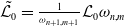For any other $\omega$ function $\omega _{n,m}\psi _{0,n,m}$ satisfies equation $\tilde {\mathcal L}_0\psi =0$ , where $\tilde {\mathcal L}_0=\frac {1}{\omega _{n+1,m+1}}{\mathcal L}_0\omega _{n,m}$ is gauge-equivalent to ${\mathcal L}_0$ and therefore has the same series of Laplace invariants. This completes the proof of Theorem 5.

In the discrete case, it is also possible to express in terms of functions (5.1) not only the general solution (5.2), but also the coefficients of the operator ${\mathcal L}_0$ . The functions $A_{0,n,m}$ and $B_{0,n,m}$ can be expressed in terms of (5.1) using the expansion of determinant (5.2) along its first row; see Remark 6. The coefficients of ${\mathcal L}_0$ can be expressed in terms of them.

Proposition 7. If the general solution of the equation $L_0\psi =0$ with the Laplace series terminating at the terms $r$ and $-s$ is given by ( 5.2 ), then the coefficients of the operator ${\mathcal L}_0$ have the form

(5.17) \begin{equation} a_{n,m}=-\frac {A_{s,n+1,m+1}}{A_{s,n+1,m}},\ b_{n,m}=-\frac {B_{r,n+1,m+1}}{B_{r,n,m+1}},\ c_{n,m}=\frac {\sum \limits _{i=0}^s A_{i,n+1,m+1}+a_{nm}\sum \limits _{i=0}^s A_{i,n+1,m}+b_{nm}\sum \limits _{i=0}^s A_{i,n,m+1}}{\sum \limits _{i=0}^s A_{i,n,m}}. \end{equation}

Proof. Consider the general solution of ${\mathcal L}_0\psi =0$ in form (5.7) and apply shifts:

\begin{align*} \psi _{0,n+1,m}&=A_{0,n+1,m} N_{n+1}+\cdots +A_{s,n+1,m} N_{n+s+1}+B_{0,n+1,m} M_m+\cdots +B_{r,n+1,m} M_{m+r}\\ \psi _{0,n,m+1}&=A_{0,n,m+1} N_{n}+\cdots +A_{s,n,m+1} N_{n+s}+B_{0,n,m+1} M_{m+1}+\cdots +B_{r,n,m+1} M_{m+r+1}\\ \psi _{0,n+1,m+1}&=A_{0,n+1,m+1} N_{n+1}+\cdots +A_{s,n+1,m+1} N_{n+s+1}+B_{0,n+1,m+1} M_{m+1}+\cdots +B_{r,n+1,m+1} M_{m+r+1}.\\ \end{align*}

Note that the expression

\begin{equation*} \tilde \psi _{0,n,m}:=\psi _{0,n+1,m+1}-\frac {A_{s,n+1,m+1}}{A_{s,n+1,m}}\psi _{0,n+1,m}-\frac {B_{r,n+1,m+1}}{B_{r,n,m+1}}\psi _{0,n,m+1} \end{equation*}

does not contain the highest shifts $N_{n+s+1}$ and $M_{m+r+1}$ , that is it has form (5.7). Moreover, the substitution $N=\nu _i$ , $M=\mu _i$ for every $i=1,2,\ldots ,r+s+1$ implies that $\psi _0=0$ and, hence, that $\tilde \psi _0=0$ . Using the same argument as before, we deduce that there exists a function $\omega$ such that $\tilde \psi _{0,n,m}=\omega _{n,m}\psi _{0,n,m}$ . Hence,

(5.18) \begin{equation} \psi _{0,n+1,m+1}-\frac {A_{s,n+1,m+1}}{A_{s,n+1,m}}\psi _{0,n+1,m}-\frac {B_{r,n+1,m+1}}{B_{r,n,m+1}}\psi _{0,n,m+1}=\omega _{n,m}\psi _{0,n,m}. \end{equation}

This means that we constructed a hyperbolic second-order difference operator with a unitary leading coefficient that is annihilated by the general solution $\psi _0$ of the initial equation. Hence, we only need to prove the formula for $c_{n,m}=-\omega _{n,m}$ . Consider the particular solution that corresponds to $N_n\equiv 1$ , $M_m\equiv 0$ and substitute it into (5.18) to find $\omega$ .

6. Semi-discrete case

In this section, we briefly discuss semi-discrete analogues of the Darboux formulae. All proofs are similar to the ones in the continuous and in the entirely discrete cases.

Theorem 7. If the Laplace series of a semi-discrete hyperbolic operator ${\mathcal L}_0$ is finite, $h_r=k_{-s}=0$ for some $r,s\geqslant 0$ and the operators ${\mathcal L}_{-s+1},\ldots ,{\mathcal L}_{r-1}$ have non-zero Laplace invariants, then the general solution of difference equation ${\mathcal L}_0\psi =0$ has the form

\begin{equation*} \psi _{0,n}=A_{0,n} N_n+A_{1,n} N_{n+1}+\cdots +A_{r,n} N_{n+r}+B_{0,n} X+B_{1,n} X'+\cdots +B_{s,n} X^{(s)}, \end{equation*}

where $N_n$ and $X$ are arbitrary functions of variables $n$ and $x$ respectively, $A_{i,n}$ and $B_{j,n}$ are some particular functions depending on the coefficients of the initial equation, and $A_0\ne 0$ , $A_r\ne 0$ , $B_0\ne 0$ , $B_s\ne 0$ .

If a hyperbolic equation ${\mathcal L}_0\psi =0$ admits a solution of the form ( 5.7 ), where $A_0\ne 0$ , $A_r\ne 0$ , $B_0\ne 0$ and $B_s\ne 0$ , then its Laplace series is finite, $h_r=k_{-s}=0$ , and the operators ${\mathcal L}_{-s+1},\ldots ,{\mathcal L}_{r-1}$ have non-zero Laplace invariants.

Theorem 8. Let ${\mathcal L}_0$ be a hyperbolic differential-difference operator with a finite Laplace series where $h_r=k_{-s}=0$ for some $r,s\geqslant 0$ . Then there exist functions

(6.1) \begin{equation} \nu _{1,n},\nu _{2,n},\ldots ,\nu _{r+s+1,n}\quad \hbox{and}\quad \xi _1 (x),\xi _2 (x),\ldots ,\xi _{r+s+1} (x) \end{equation}

of one discrete variable and a function $\omega _n=\omega _n(x)$ such that the general solution of ${\mathcal L}_0\psi =0$ is given by the determinant formula

(6.2) \begin{eqnarray} \psi _{0,n}=\omega _{n}\cdot \det \left ( \begin{array}{cccccccc} X & X' & \ldots & X^{(s)} & N_n & N_{n+1} & \ldots & N_{n+r}\\ \xi _1 & \xi '_1 & \ldots & \xi ^{(s)}_1 & \nu _{1,n} & \nu _{1,n+1} & \ldots & \nu _{1,n+r}\\ \xi _2 & \xi '_2 & \ldots & \xi ^{(s)}_2 & \nu _{2,n} & \nu _{2,n+1} & \ldots & \nu _{2,n+r}\\ \vdots &&&\vdots &&&&\vdots \\ \xi _{r+s+1} & \xi '_{r+s+1} & \ldots & \xi ^{(s)}_{r+s+1} & \nu _{r+s+1,n} & \nu _{r+s+1,n+1} & \ldots & \nu _{r+s+1,n+r}\\ \end{array} \right ), \end{eqnarray}

where $N_n$ and $X(x)$ are arbitrary functions of one variable.

For any two families of linearly independent functions of one variable ( 6.1 ) and for any function $\omega _n=\omega _n(x)$ , there exists a hyperbolic differential-difference operator ${\mathcal L}_0$ with a finite Laplace series that terminates at the terms $r$ and $-s$ such that formula ( 6.2 ) provides the general solution of ${\mathcal L}_0\psi =0$ .