

Introduction
Potential water scarcity due to climate change is of great concern in California. Expected variations in temperature and precipitation as climate changes, coupled with a changing population, droughts, and wildfire risks to watersheds on public lands, are putting increasing pressure on water resources in the state. As a result, there is a growing interest among policy makers and land managers to understand how the economic value of water-provisioning services from public lands may vary through the 21st century in California's drought-prone environment. This policy interest is heightened by concerns with how climate change will affect future water supply in the state.
Climate projections for Southern California are partially explained by its Mediterranean-type climate. Global climate models predict that most areas with Mediterranean-type climates will become drier (Polade et al. Reference Polade, Gershunov, Cayan, Dettinger and Pierce2017). Correspondingly, climate change is expected to affect precipitation patterns in California (Cvijanovic et al. Reference Cvijanovic, Santer, Bonfils, Lucas, Chiang and Zimmerman2017), resulting in adverse effects for the supply of surface water in the state's major hydrological basins (Dettinger, Udall, and Georgakakos Reference Dettinger, Udall and Georgakakos2015; Vicuna et al. Reference Vicuna, Maurer, Joyce, Dracup and Purkey2007). Basin-level assessments have shown that water supplies from hydrological basins that supply Southern California are vulnerable to the effects of climate change (e.g., Foti, Ramirez, and Brown Reference Foti, Ramirez and Brown2014; Pagán et al. Reference Pagán, Ashfaq, Rastogi, Kendall, Kao, Naz and Pal2016). National forests represent an important source of water for downstream communities in Southern California, and lands managed by the U.S. Department of Agriculture (USDA) Forest Service supply about 47 percent of surface water supply in California (Brown, Hobbins, and Ramirez Reference Brown, Hobbins and Ramirez2008; Brown et al. Reference Brown, Froemke, Mahat and Ramirez2016). Additionally, increasing variability in water supply is a concern, as it has implications for other salient issues in the region, such as how ecosystems, water, and fire can be managed (Sawyer, Hooper, and Safford Reference Sawyer, Hooper and Safford2014, p. 6).
A priority for policy makers is managing demand for water. The demand for and use of residential water will change because population size and preferences are evolving. Demand management and water conservation policies have been in place for many years, resulting in continual decreases in per capita water consumption in the region; for example, the Los Angeles Department of Water and Power delivered 112 gallons of water per capita in 2017–2018, one of the lowest per capita rates of any major U.S. city, reinforcing the overall decline in per capita use. As such, total water consumption in Los Angeles was lower in 2017 than in 1970, despite an increase of more than one million people over that 47 year period (Los Angeles Department of Water and Power, 2019).
This paper focuses on how residents in urban areas who use municipally treated water will be affected by changes in supply caused by climate change. Urban areas may face challenges in providing fresh water to their growing populations as a result of “unprecedented hydrologic changes due to global climate change” (McDonald et al. Reference McDonald, Green, Balk, Fekete, Revenga, Todd and Montgomery2011, p. 6312). As decision makers try to evaluate trade-offs between policy alternatives, however, they have limited economic information about how ecosystem service values will be affected by climate change. We estimate the effects of climate change on the economic value of raw, untreated water from public lands—in particular, from the San Bernardino National Forest, which is administered by the USDA Forest Service—throughout the 21st century, reporting results for every decade. A better understanding of how variations in water supply affect welfare may help public land managers and water utility managers evaluate potential trade-offs from land management activities that affect water supply, alternative water supplies or infrastructure investments, and pricing structures.
We have chosen Southern California because it differs from other Mediterranean-type locations in a few ways. For example, it experiences more intense summer droughts compared to other Mediterranean-type locations, with only 5 percent of annual precipitation occurring in the summertime (Cowling et al. Reference Cowling, Ojeda, Lamont, Rundel and Lechmere-Oertel2005). Precipitation occurs more infrequently in Southern California than in other Mediterranean-type locations (Cowling et al. Reference Cowling, Ojeda, Lamont, Rundel and Lechmere-Oertel2005), and it has the most variable rainfall regime of the world's Mediterranean-type climate zones. Wildfires also pose a threat to water supplies in Southern California. Wildfires are a common occurrence in Southern California and can affect the ability of public lands to provide water as an ecosystem service. For example, the 2009 Station Fire in the Angeles National Forest has been the largest in Los Angeles County to date, burning 160,000 acres and considerably disturbing water provisioning from the affected watersheds.
The San Bernardino National Forest is the focus of this study because it provides the main source of water for water retailers serving four communities in Southern California: San Jacinto, Riverside, Colton, and Redlands.Footnote 1 San Bernardino National Forest is one of four large national forests in Southern California—along with Los Padres, Angeles, and Cleveland national forests—and may therefore inform policy decisions for the rest of the region. These four national forests cover an area of 14,335 km2 and generate a mean annual water supply volume of 2.05 billion m3 (Brown et al. Reference Brown, Froemke, Mahat and Ramirez2016)—amid a population of almost 23 million people (U.S. Census Bureau 2014). Landscapes in San Bernardino National Forest are largely semi-arid with Mediterranean-type ecosystems and significant chaparral coverage.
The purpose of this paper is to estimate the economic value of water for household use supplied by the San Bernardino National Forest. The study seeks to estimate the effects on consumer welfare from variations in water supply due to climate change through the 21st century. The focus here is on use values for municipally-treated water by urban households. Other sectors (e.g., agriculture and industrial) are also important users of water in Southern California, although analysis of use values for these sectors is left to future research. Since water supply and use vary over time, we examine the timing of resource availability. The study estimates the value of water by projecting changes in the volume of surface water supplied by the San Bernardino National Forest into the future and estimating the corresponding welfare effects. We are able to estimate welfare changes by coupling projections of surface water runoff from a regionally calibrated dynamic global vegetation model, with a range of estimates of the price elasticity of demand for surface water from the literature.
This study extends previous work in several important ways. First, to our knowledge this is the first study to address how the economic value of water will change through the 21st century due to climate change in Southern California. Second, we project future water supply using a biophysical model under 28 different possible climate future projections, reported by decade, which has not been done previously for California, nor other Mediterranean-type areas. Finally, we generate corresponding estimates of water provisioning ecosystem service by decade from 2020 until the end of the century, for a wildfire and drought-prone ecosystem.
Importance of Ecosystem Service Valuation for Water in the National Forests
National forests connect and encompass watersheds as well as terrestrial and coastal ecosystems, producing a variety of environmental services, including the supply and purification of fresh water. Public concern about adequate supplies of clean water and protection of water provisioning services for nearby residents contributed to the establishment of federally protected forest reserves in the United States (USDA Forest Service 2000; Steen Reference Steen2004, p. 36). A significant source of annual freshwater in the United States originates from forests—46 percent—out of which about 14 percent originates from national forests (Brown et al. Reference Brown, Froemke, Mahat and Ramirez2016); about 80 percent of streams in the U.S. originate from public and private forests (USDA Forest Service 2000). There are 81 national forests in the western U.S., collectively occupying 573 thousand km2 (57,300,000 ha). These national forests provide an annual average water yield of 230 billion m3; in the western United States—comprised of Arizona, California, Colorado, Idaho, Montana, New Mexico, Nevada, Oregon, Utah, Washington, and Wyoming—national forests provide 49 percent of the mean annual water supply (Brown et al. Reference Brown, Froemke, Mahat and Ramirez2016).
Given that national forests are a vital source of fresh water in the West, their management in semi-arid Southern California plays an even more important role in the provision of water as an ecosystem service. Indeed, forest plans explicitly state the need to balance the needs of downstream users and in-stream resource needs when engaging in land management activities (USDA Forest Service 2005a, p. 11). For example, forest managers cooperate with other water agencies to engage in projects to maintain the provision of water to users and for resource needs (USDA Forest Service 2005b, p. 23). They must weigh trade-offs between competing uses for the water—whether for downstream water retailers, on-site recreational purposes, stream diversions on the forest for water withdrawals by private companies (James Reference James2018), and in-stream ecological and habitat needs (USDA Forest Service 2005c, pp. 36–37). Forest managers at the agency must also consider the sustainable use of multiple goods and services provided by national forests under the Multiple-Use Sustainable Yield Act of 1960;Footnote 2 this law includes watershed uses among timber, range, recreation, wildlife, and fish-related uses.
This study focuses on raw, or untreated, water from the San Bernardino National Forest, which covers 2,723 km2 and is located about 145 km east of Los Angeles. This national forest contains Mount San Gorgonio, the tallest peak in Southern California, at 11,502 feet (3,506 m). It includes several mountains—the San Gabriel, the San Bernardino, San Jacinto, and the Santa Rosa Mountains—which encompass several critical watersheds. San Bernardino National Forest offers year-round recreational opportunities, such as water-based recreational activities at multiple lakes and skiing in the mountains. It also provides valuable watershed protection. Nevertheless, recent analysis of weather station data near the Angeles and San Bernardino National Forests indicates that “year-to-year variability in precipitation has been increasing over the course of the last century at these stations” (Sawyer, Hooper, and Safford Reference Sawyer, Hooper and Safford2014, p. 6).
Literature Review
There are several challenges involved in accurately valuing water from national forests, such as trying to price nonmarket values, complex aquatic and riparian ecosystems, and the interrelated values between water and watershed services; these obstacles often result in the undervaluation of water in management decisions (Berry, Reference Berry2010). In Southern California, the challenges of droughts, wildfires, ageing infrastructure and leakage, population growth, environmental requirements, economic development, and budgetary constraints compound the region's vulnerability to climatic changes. As far back as 2009, the California Environmental Protection Agency and the California Energy Commission sponsored a study to investigate the effect of climate change on a wide range of ecosystem services in the state that included two case studies: one for quantifying water supply for a cultural service (skiing) and the other for in-stream flows for fresh water fish (California Climate Change Center, 2009). The study did not, however, examine water for municipal purposes, nor did it quantify economic values.
Few studies quantify multiple economic benefits from forests with Mediterranean-type climates. Watershed protection and watershed-related services have been considered as components of forest ecosystem service provision in European and North African Mediterranean-type climates, although water supply for household use was not explicitly considered (Merlo and Croitoru Reference Merlo and Croitoru2005). Water is recognized as an important constraint when managing Mediterranean-type forests for multiple objectives under changing climate and wildfire conditions (Palahi et al. Reference Palahi, Mavsar, Garcia and Birot2008). A challenge with such studies is that it is difficult to weigh trade-offs among multiple objectives without quantifying values (or other means of comparison).
Climate-induced changes in water availability affect welfare in a variety of ways for both water retailers and their customers. Reduction in revenues, higher water rates, costs of changing behavior to constrain water use, infrastructure investments, expenditures on water-saving devices, and new municipal codes and standards are examples of initiatives that affect economic welfare that may result from climate change. These changes in welfare can be quantified in terms of changes in economic benefits or opportunity costs. Where water use approximates a private good—as in the case for our study of treated water consumed by single family households—“either in the production of goods and services or in the satisfaction of individual wants and needs…the estimates of the change in [the economic value or welfare] can be derived from an analysis of consumer…water demand and cost schedules” (Hurd and Rouhi-Rad Reference Hurd and Rouhi-Rad2013, p. 577).Footnote 3 Buck et al. (Reference Buck, Auffhammer, Hamilton and Sunding2016) employ a utility fixed-effects model to measure welfare losses due to a 30-percent decrease in water supply; they conclude that one of the main welfare results indicates that when volumetric rates carry a portion of the fixed costs, average welfare losses increase significantly with volume shortages.
Jenkins, Lund, and Howitt (Reference Jenkins, Lund and Howitt2003) follow this general approach by measuring welfare changes in a California context. They make use of the California Value Integrated Network (CALVIN) model, an economic-engineering optimization model of California developed at the University of California, Davis, to estimate economic loss functions due to anticipated drought-induced water shortages. The authors focus on the welfare effects on urban water users in California in 2020 due to water shortages relative to 1995. By integrating relevant areas under the demand curve, they estimate economic losses from urban water scarcity to average $1.6 billion per year in 2020.Footnote 4
Young and Gray (Reference Young and Gray1972), Young (Reference Young2005), and Young and Loomis (Reference Young and Loomis2014) cite earlier work by James and Lee (Reference James, Lee, Chow, Eliassen and Linsley1971) as the basis of their approach to derive an estimated value of treated water consumed by single family households by examining a change in supply. They estimate changes in consumer surplus due to a change in water supply in one period, holding water price constant. The focus is on consumer surplus since average cost pricing is assumed—common to the water use literature—thus producer surplus is expected to be zero. They apply the standard formula for the integral of a demand function by inferring an empirical demand function from an observed price-quantity point on that demand curve and an assumed price elasticity of demand for urban water. The gross economic value of a change in water availability is quantified by integrating the demand function for the specified quantity change. Consumer surplus is then determined by subtracting the cost of storing, treating, and delivering the water to urban households. In the third and final step, leakage costs are subtracted from the consumer surplus to arrive at the economic value of raw or untreated water. The present study follows Young and Loomis (Reference Young and Loomis2014) as well as the approach outlined by Griffin (Reference Griffin1990), in which he builds upon this earlier work but assumes an explicit functional form while examining welfare changes due to increases in water supply over multiple periods and explicitly allows prices to increase over time.
Methods
In this study, the economic value of raw water is estimated in two stages. First, the quantity of water by decade from the San Bernardino National Forest is projected for the 21st century via a dynamic vegetation model, driven with climate projections from multiple global circulation models. Second, these water quantity projections are coupled with price-quantity data representing demand for municipal water by single family households. This two-step method allows us to apply a modified version of an existing valuation method to generate a trajectory of changes in consumer surplus due to variations in water supply caused by climate change. This adjusted consumer surplus is used to calculate the economic value of water from San Bernardino National Forest associated with projected water volume changes.
Generating Water Provision Projections by Decade
The first step of the method is to generate projections of the volume of surface water runoff by decade through the 21st century. These projections are generated using the MC2 dynamic global vegetation model (Bachelet et al. Reference Bachelet, Lenihan, Daly, Neilson, Ojima and Parton2001), which has been successfully applied at the regional scale (Case et al. Reference Case, Kerns, Kim, Day, Eglitis, Simpson, Reigel, Halofsky, Peterson and Ho2018; Kim et al. Reference Kim, Kerns, Drapek, Pitts and Halofsky2018). MC2 was calibrated to Southern California using multiple observation data sets, including net primary productivity, carbon stock estimates, and wildfire regimes. MC2 models vegetation response to climate change over time by simulating the processes that govern ecosystem carbon and water cycling, vegetation biogeography, and wildfire occurrence and effects. Model outputs include spatial distribution of potential natural vegetation and stream flow.
MC2 represents the landscape as a grid, and simulations are driven by downscaled monthly climate projections derived from 28 general circulation models (GCMs) simulating representative concentration pathway 4.5 (RCP4.5), a “medium” stabilization emissions scenario (van Vuuren et al. Reference van Vuuren, Edmonds, Kainuma, Riahi, Thomson, Hibbard and Rose2011, p. 11). Downscaled climate projections for the 28 GCMs are drawn from a published data set, NEX-DCP30 (Thrasher et al. Reference Thrasher, Xiong, Wang, Melton, Michaelis and Nemani2013), which uses a statistical downscaling method called the Bias Correction-Spatial Disaggregation (BCSD) to transform coarse spatial scale GCM output published by the Coupled Model Intercomparison Project 5 (CMIP5; Taylor, Stouffer, and Meehl Reference Taylor, Stouffer and Meehl2012) to a fine scale (30 arc-seconds, or approximately 800m). MC2 parameters were adjusted so that model outputs for plant productivity, carbon stocks, biogeography, and fire regime align with observed values.
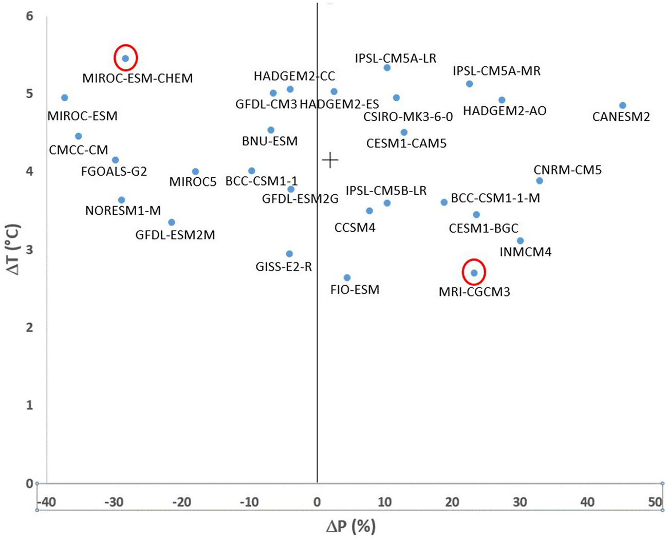
Although the GCMs simulate one climate change scenario, the RCP4.5, the simulated future climate projections vary widely in temperature and precipitation (see the appendix, Figure A1), and, in turn, streamflow simulated by MC2. In other words, the 28 streamflow projections simulated by MC2 capture a range of uncertainty arising from GCMs. We analyze the ensemble of 28 streamflow projections for the study area. In each decade we calculate annual flow volumes from each of the 28 simulated streamflow projections and calculate the ensemble mean by decade, to be used in the economic valuation.
In addition to reporting on the mean of the ensemble of 28 future projections, we also present results for two individual GCMs as case studies. The variability among GCMs can be summarized in terms of projected changes in temperature and precipitation. A “warm-wet” model—MRI-CGCM3—was selected to represent a moderate temperature increase (about 1.4⁰ C) and large precipitation increase (about 18%). A “hot-dry” model—MIROC-ESM—was selected to represent the high end of temperature increases (about 3.0⁰ C) and large precipitation decreases (about −30%). (See the appendix, Figure A1, for the distribution of the 28 model projections in temperature-precipitation change space.)
We make simplifying assumptions about the hydrological model in the study area to relate supply from the national forest to downstream users. First, the model assumes that the projected average annual water flows from San Bernardino National Forest is available to the water retailers during the same decade; that is, we assume there is no lag between the provision and availability of the water (e.g., due to the timing of groundwater infiltration) at decadal time steps. Second, we assume that water utilities in the study area face stable groundwater tables over time such that water pumped from groundwater represents recent infiltration from the national forest in the same decade.Footnote 5
Developing Economic Valuation Projections by Decade
In the second step, the economic value of water is estimated. Specifically, the economic value of raw (untreated) water or the at-source value of water from San Bernardino National Forest is determined; this value is of interest as it is the most pertinent value when assessing trade-offs between different uses and non-uses of water from public lands. This category is differentiated from at-site water, which is defined to be the water delivered to urban customers such as single family households by a water retailer; at-site water includes conveyance, treatment, and distribution characteristics. Although these two are different economic goods, an empirically based approach can be used that imputes the consumer surplus from at-site water demand to derive the value of the at-source value of water (Young and Loomis Reference Young and Loomis2014). As Young and Loomis (Reference Young and Loomis2014, pp. 447–448) state, although often the most desired economic value for investment and reallocation appraisals is an at-source value, in “contrast, the most readily observable value is [an] at-site value, the willingness-to-pay at the point of use…[by]…the household.”
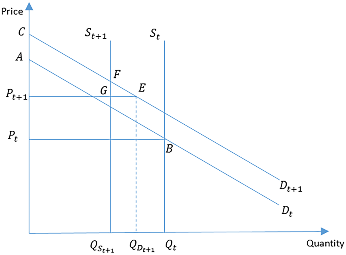
Conceptually, consider supply, demand, and price for at-site water, and how consumer surplus changes over time, in Figure 1. Demand changes over time due to changes in population and per capita consumption. At time t, the water supplied to single family households is S t, the demand for water by single family households is given by D t, the price the water retailer charges is P t, and the corresponding quantity demanded is Q t. Consumer surplus is given by the area ABP t. In the next time period, suppose demand shifts to D t+1, and price is administratively set at P t+1; at this price, the quantity demanded is $Q_{D_{t + 1}}\comma \;$ and the corresponding consumer surplus is CEP t+1. Assume in period t + 1 the supply of water decreases to S t+1 due to the effect of climate change; now consumer surplus is CFGP t+1, resulting in a decrease in welfare equivalent to FEG. This area, FEG, is the welfare measure used to calculate the change in use value of water in this study.
Welfare changes from water supply and shifts in demand
This study follows the approach outlined by Griffin (Reference Griffin1990) in estimating demand functions for each decade in the 21st century to then derive urban residential water values for households that receive their water from San Bernardino National Forest, and ultimately at-source raw water values, the ecosystem service provided by the national forest. In this article, assumptions specific to the study area are used to construct these demand functions. Young and Gray (Reference Young and Gray1972), Young (Reference Young2005), and Young and Loomis (Reference Young and Loomis2014) outline a succinct approach, which we apply to our study context, to estimate an at-source value of residential water that requires four data items:
○ a price-quantity point—an observed price in effect during a specified period,
○ the corresponding water deliveries observed during that same period,
○ a hypothetical change in quantity that is to be valued, and
○ the assumed price elasticity of demand.
The approach in this study accounts for several factors that change over time, captured in Figure 1. Specifically, the model accounts for population growth, per capita consumption limits mandated in California, other demand curve shifters, growth in prices, and leakage from the municipal water systems. Whereas Young and Loomis (Reference Young and Loomis2014) assume a constant elasticity of substitution functional form for demand, we follow Griffin (Reference Griffin1990) in using a Cobb-Douglas functional form, as it is commonly employed in demand estimation, it meets the requirement for a constant elasticity of substitution function, and as Griffin notes, the approximated function lies in the correct orthant with positive prices and quantities.Footnote 6 Although his objective is to value increases in water supply, we apply Griffin's approach here to also value decreases in supply.
The single family household demand for urban water is assumed to be:

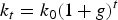
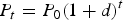
where (Q, P) is the quantity and price of residential water, k is a constant, and ɛ is the price elasticity of demand for residential water. The observed quantity, price, and price elasticity of demand for the base period (2015) are denoted Q 0, P 0, and ɛ 0, respectively. Rearranging Equation (1) gives the following initial value of the constant in the base period:

Following Griffin (Reference Griffin1990), the price elasticity of demand for treated water by single family households is assumed to be constant along the curve and over time, and not equal to 1; demand will shift outward over time due to changes in the population and per capita consumption growth rates. Demand by single family households in period t is given by

and
where g incorporates both the expected population and per capita consumption growth rates, which may be positive or negative. This is an improvement over the model proposed by Griffin (Reference Griffin1990), which only accounts for the population growth rate. Note that since k changes over time, the demand curve shifts over time as well. Inverse demand is given by:
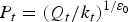
The inverse of the price elasticity of demand, ${1 /{\varepsilon _0}}\comma $ in Equation (5) is referred to as the price flexibility of demand. This expression reflects the “proportional change in value to users from a given change in quantity consumed, the relationship of interest in many water valuation contexts” (Young and Loomis, Reference Young and Loomis2014, p. 475).
In period t, the quantity demanded by single family households is Q t, so in the base period, the quantity demanded is given by Q 0. In time t, the quantity demanded by households at the prevailing price is a, whereas the amount supplied to the household sector by a water retailer is b. When b > a, there is a supply surplus, and if price adjusts to clear the market, total benefits to residents is given by V t, which is equivalent to the area under the demand curve, specified by:
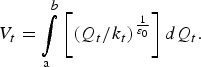
If the supply available to households in time t is less than the quantity demanded at the prevailing price in time t, such that b < a, then the welfare decrease is given by the negative of equation (6), as the order of the limits is reversed.
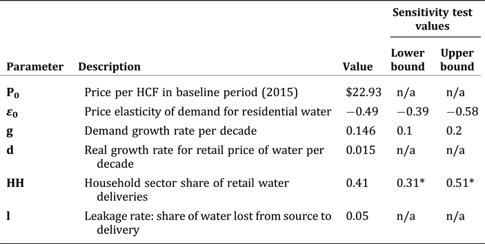
The reference price series is assumed to be an administratively set reference price that increases over time, reflecting trends in California and especially in Southern California. Price is calculated as:
where d is the growth rate for price or water rate charged to single family households in the study area. This rate will reflect increases in marginal cost for sourcing water, infrastructure investments, and other associated costs for operations and maintenance. This reference price trend set by the water retailers is assumed to be exogenous to the final supply in any time period and exogenous to households, but the retailers pick the rate d to reflect their expectations of trends. For the purposes of valuing supply changes, we assume that if a surplus of water is realized in any period, price is allowed to fall to clear the supply for that period, and conversely, if there is a shortage, the price is held at the reference level and rationing is used to address the shortage.Footnote 7
In addition to the value of treated water for households, this study also estimates the value of the raw water from San Bernardino, or the at-source value of water from San Bernardino National Forest. To derive this value, the approach expounded by Young and Loomis (Reference Young and Loomis2014) is followed. Note that demand studies for municipally treated tap water measure the willingness to pay for services to capture, transport, treat, and store the water in addition to the water itself. Thus, the costs associated with these services must be deducted from the estimated willingness to pay for tap water in order to correctly impute the value of raw water. It is assumed that if the treated water is priced to fully recover its associated costs—so full-cost pricing with no producer surplus—then the average revenue can be subtracted from the total willingness to pay to arrive at the net consumer surplus imputable to raw water. The water retailers examined in this study are assumed to set water rates for household customers at full cost.
Therefore, assuming P t is the average cost of water charged to households, P t × Q b is equal to the amount paid for the final water quantity. Let C t be the change in consumer surplus associated with the increase in quantity from $Q_{a}$ to $Q_{b}$
 , then the cost associated with this change in quantity is subtracted from V t, the total benefit or value of the treated water:

This change in consumer surplus needs to be further adjusted to account for losses due to leakages and errors with meters. A per unit value of consumer's surplus final value of raw water is given by:
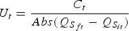
and finally, the value of at-source (raw) water, or the value of the ecosystem service from the national forest, is calculated as:
where R t is the per unit net benefit or value of raw water to the water retailer's customers in period t, and l 0 is the proportion of water lost due to leakage or meter errors or pilferage in the base period, and is assumed to remain constant over time.
Model Inputs and Parameters
Parameterizing the model, described earlier, requires choices of several parameters describing the supply and demand for water in this particular basin and for the water retailers that rely on water from San Bernardino National Forest. Furthermore, it requires assumptions to characterize how certain components of the model will change over time.
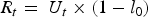
Table 1 reports key model parameter values used to generate estimates, and the ensuing discussion details the sources and rationale for each parameter. In general, we opt for simple assumptions, particularly related to temporal dynamics. These assumptions are guided by relevant literature or public documents where possible, although in some cases only limited guidance is available. In this sense, the assumed model parameters may be considered a first approximation, with the potential to incorporate better information or more nuanced assumptions when available.
Parameter Values Used for Model and Sensitivity Tests
Note: *For the purposes of the sensitivity tests, the lower bound reflects a sensitivity test where the household share of retail water deliveries declines each decade by about 1.4 percentage points each decade, ending at the lower bound of hh = 0.31. The upper bound indicates a sensitivity test where the household share increases each decade by about 1.4 percentage points, ending in the last decade with the upper bound of hh = 0.51.
Pricing Structure, Initial Price, and Price Elasticity of Demand for Residential Water
Price in the base period (2015) is the average price charged to households by the water retailers in four cities—Riverside, San Jacinto, Redlands, and Colton—because the water retailers that serve these communities get their entire supply from the San Bernardino National Forest, either as surface water or ground water, or both.Footnote 8 Their water sources are specified in their 2015 Urban Water Management Plans. Riverside and San Jacinto are located in Riverside County, while Colton and Redlands are in San Bernardino County. Some rely on groundwater exclusively (e.g. Riverside and San Jacinto) while others use a combination of surface and ground water (e.g. Redlands). This price represents the cost of treating, storing, and delivering the water. Derivation of the current price is explained in further detail later.
With respect to prices, three types of pricing schemes for water to residential households are observed in California: 1) uniform pricing, where each household pays a fixed price per hundred cubic feet; 2) tiered or block pricing, where the price per hundred cubic feet (HCF) for the household depends upon the amount of water consumed, and 3) allocation-based pricing, which is a type of block pricing that accounts for household characteristics (Baerenklau, Schwabe, and Dinar Reference Baerenklau, Schwabe and Dinar2014). All four municipalities use a tiered water-pricing scheme with increasing block rates. In the case of increasing block rates, the first few HCFs are priced relatively low, whereas subsequent HCFs are priced higher such that the per-HCF price increases in conjunction with consumption. All household customers are charged the tier 1 amount to cover fixed costs regardless of the amount of water consumed, even when consumption declines, such as during shortages. Water retailers have been contending with declining per capita consumption for many years and thus have increasingly been moving towards tiered pricing structures or water budgets to maintain revenues.
The price used for the base period (P 0) is the average water rate of the four municipalities and is calculated as follows. First, we take the retailer's per capita gallon consumption by single family households for 2017–2018Footnote 9 and multiply this by the average number of people per household for the municipality as recorded by the most recent United States Census; this household consumption is converted to HCFs. Then, this average household consumption is multiplied by the relevant tiered rate(s) for a single family household to arrive at an average cost per HCF per household. The average water rate per HCF across these four municipalities is $22.93 per HCF in period P 0.Footnote 10
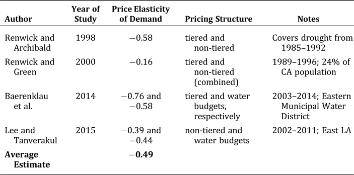
Table 2 shows the price elasticity of demand estimated in studies of residential demand for urban water in Southern California. The average of these (−0.49) is used in estimating the economic value of water, in Equations (2), (3), (5), and (6), or: ɛ 0 = −0.49. This value falls in the range of residential water price elasticities reported by Espey, Espey, and Shaw (Reference Espey, Espey and Shaw1997), and is close to their mean estimate of all studies of −0.51.
Price Elasticity of Demand for Municipally Treated Water in Southern California
Projected Price in 21st Century and Demand for Residential Water
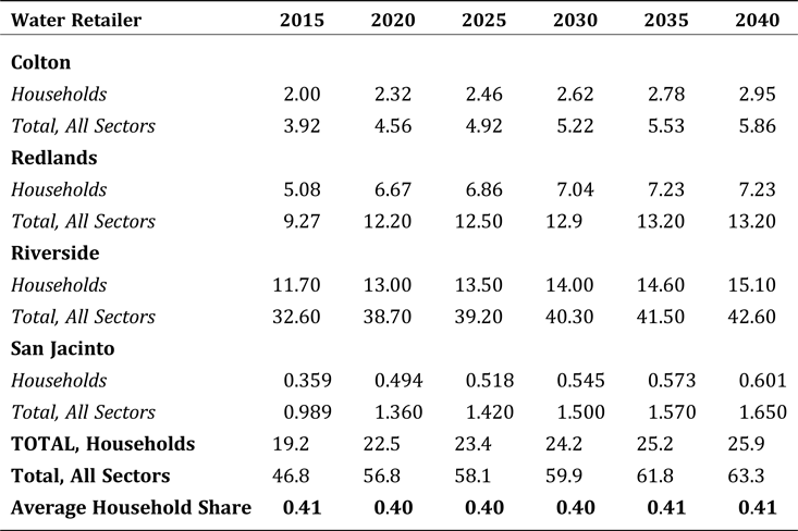
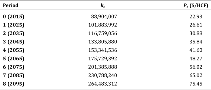
The constant in the base period, k 0, in Equation (2) is calculated using the average price in the base period ($22.93), the total reported deliveries to the household sector, and the price elasticity of demand. Water retailers are required by the state to develop and submit urban water management plans every five years in accordance with the California Urban Water Management Planning Act of 1983 (City of Riverside 2016; City of San Jacinto 2016; San Bernardino Valley Municipal Water District 2016). Deliveries to households by the four retailers—which we use as the initial quantity demanded—totaled about 19.2 million HCF in 2015 (see the appendix, Table A1 for retailer deliveries used to calculate initial demand).
The growth rate for the constant, g, as specified in Equation (4), is derived from projected demand in the 2015 urban water management plans, and includes changes in population and per capita consumption. Retailers are required to forecast their demand over the next 25 years and report these projections in their water management plans. In making these projections, the retailers include both population growth and changes in per capita consumption that align with state-mandated limits; for example, in 2018 California mandated a 55-gallon per capita per day limit for indoor use. Under Assembly Bill 1668 and Senate Bill 606, water utilities must meet this limit on average across all their customers or they could face fines; this limit is reduced to 52.5 gallons by 2025, and 50 gallons by 2030. If the 50 gallons/capita daily limit is maintained, then by 2060—halfway through the 80 year time period being studied—the total projected to be consumed is about 2.3 billion gallons per day, or about 6,951 acre-feet per day; the comparable figure from 2015 is about 17,499 acre-feet per day, representing a decrease of about 40 percent over the 45-year period between 2015 and 2060. This may be achievable, as the total daily consumption decreased by about 17 percent over the 15-year period 1990 to 2015 (California Department of Finance 2007; California Department of Finance n.d.; Mount and Hanak Reference Mount and Hanak2019). Moreover, it has been noted that even after the last drought ended in 2017, there have been indications that per capita consumption has remained lower than before the drought in some areas of Southern California.Footnote 11
In their 2015 urban water management plans, the retailers have assumed that they will meet these caps. The discrete growth rate for the 25-year period is calculated from the continuous growth rate for each individual retailer's projected data series, and then the average of their discrete growth rates is computed.Footnote 12 This average discrete annual growth rate from the four water retailers is calculated and then applied to the 10-year periods from 2020 to 2099 for a growth rate (g) of 0.146 per decade.
The retail price of water paid by single family households in each period is calculated according to Equation (7), where the real growth rate d is set to 0.015 (Metropolitan Water District of Southern California 2015). This rate is used by the Metropolitan Water District of Southern California, a major wholesaler of water in California that is one of 29 long-term Water Supply Contractors that purchase water directly from the California Department of Water Resources’ State Water Project. It delivers an average of 1.5 billion gallons of water per day to most of the southern coastal region (Metropolitan Water District of Southern California, 2019); although all four water retailers in this study get their water from San Bernardino National Forest, Riverside can access water from the Metropolitan Water District if necessary.Footnote 13 Prices are assumed to increase, reflecting actions by wholesalers such as the Metropolitan Water District and retailers.Footnote 14 Prices used in each decade, along with calculations of the demand constant k, are reported in the appendix, Table A1.
The quantity demanded by single family households at the prevailing administrative price in each period is calculated using Equation (3). To determine whether there is a shortage or surplus of water for single family households in period t, this forecasted quantity demanded is then compared to what is available to the water retailers that can be allocated to single family households.
To determine the quantity of water available for households in period t, the projected water demanded by all sectors that receive water deliveries by the water retailers is calculated. We assume that the ratio of household demand to total demand among all sectors in 2015 will remain constant in the future and that demands on supply from outside the retail water utility are negligible. Specific information about where the raw water from the national forest eventually goes is not available from the USDA Forest Service nor the retailers’ reports.
In 2015 water deliveries to household users comprised approximately 41 percent of deliveries to all sectors (about 19.2 million HCF for households and 46.8 million HCF to all sectors). Delivered volumes from 2015 are drawn from the water retailers’ respective urban water management plans; retailers must report their deliveries to all sectors that they service, such as single family households, multifamily homes, agriculture, industry, and government. Under this assumption, dividing estimated quantity demanded by households in any decade by 0.41 yields the total demand among all sectors. Total demand can then be compared to total projected surface water flows from San Bernardino National Forest to determine whether, on average, there will be an expected supply shortage or surplus.
Finally, to derive the raw water values using Equation (10), the average leakage rate of the four water retailers reported in their respective urban water management plans; the leakage rate is 5 percent and is assumed to be constant through to the end of the century.
Results
Table 3 reports average annual surface water flows by decade for the ensemble mean and the two bookend GCMs. On average, the ensemble mean of water available from the San Bernardino National Forest ranges from about 50 million HCF at the beginning of the century to about 76 million HCF at the end of the century. Individual GCM projections, however, are relatively more variable; for instance, on average, the warm-wet GCM exhibits slightly lower water availability compared with the ensemble mean and some decades are projected to drop well below average. The hot-dry GCM, on average, projects about half the water available under the ensemble mean but with larger decade-over-decade swings in availability.
Projected Average Annual Water Volume from San Bernardino National Forest Through 21st Century under Alternate GCMs, by Decade (millions of HCF)

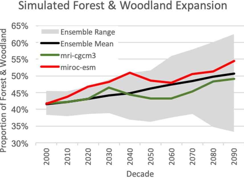
An interesting feature of generating the water volumes from the MC2 model is that the vegetation response to climate change is highly dynamic over time, due to simulated interactions between climate, vegetation, and fire. In MC2 simulations, a warming climate promotes greater vegetation productivity, leading to expansions of forests and woodlands, coupled with increased fire activity (see in appendix Figure A2). For example, ensemble mean water volumes are higher than both the warm-wet and hot-dry models in several decades, because both GCMs drive greater forest and woodland expansion, with more water transpired and less runoff. Simulation results suggest a large vegetation loss to fire is possible in the study area, as vegetation type conversion passes a threshold mid-century, leading to a temporary increase in runoff before burned areas are re-vegetated.
Table 4 reports average annual quantity demanded by households in each decade, the projected volume of water available to the household sector, and the projected surplus/shortage in each decade, by GCM. The point of reference in determining whether there is a surplus or shortage in each decade is the quantity demanded (column a), similar to the approach used by others (e.g., Jenkins, Lund, and Howitt Reference Jenkins, Lund and Howitt2003). For example, for the decade 2020–2029, the quantity of water demanded by households at the administrative price will be 20.4 million HCF. The ensemble mean of the GCMs projects 20.3 million HCF of water available to households from San Bernardino National Forest, resulting in a small shortage, shown in column (c); under the warm-wet and hot-dry GCMs, the amount of water available from the forest for households is projected to be a surplus of 8.8 million HCF and a shortfall of 15 million HCF, respectively.Footnote 15
Projected Average Annual Volume of Treated Water Demand, Availability, and Surplus/Shortages by Single Family Households by Decade (millions HCF)
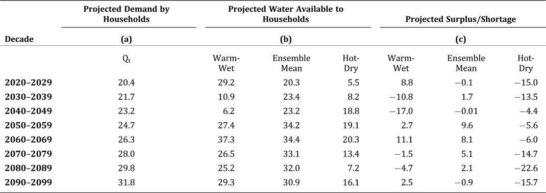
Note: Q t is from Equation (3). Perceived discrepancies due to rounding.
Table 5 presents the trajectory of changes in consumer surplus and raw water values per unit volume of water throughout the 21st century under the different GCMs (the results of estimates of equations 8 and 10). Households will experience gains in consumer surplus (positive values) in time periods when available volumes exceed demand and will experience decreases (negative values) when available water cannot meet quantity demanded.
Changes in Household Consumer Surplus in 21st Century in Response to Water Surpluses and Shortages, by Decade and GCM (‘000 $)
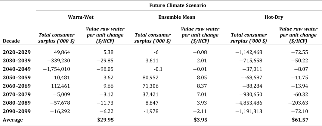
Note: Dollar values are denominated in 2018 dollars.
Negative values indicate decades when there is insufficient water to meet the demand for single family households across the four water retailers; thus, these consumer surplus figures reflect consumer surplus lost due to consumption being limited to less than the demanded volume. Positive values indicate decades when available supply exceeds demands; these values reflect the consumer surplus that could be gained if prices were allowed to adjust so demand equals supply.
Consumer surplus values reflect changes in supply, not total consumer surplus for the entire supply.
Averages are calculated using the absolute value of the raw water values.
Results indicate that water available from San Bernardino National Forest through the 21st century will largely generate positive changes in consumer surplus due to the ensemble mean supply frequently exceeding household demand. Estimated changes in consumer surplus range from a negligible decline of about $6,000 annually at the beginning of the century to a decrease of almost $2 million annually by the end of the century (in 2018 dollars); note that by mid-century the maximum increase is almost $81 million. These changes in welfare for the ensemble mean are determined by shortages and surpluses due to variations in climate, as well as demand being constrained by price increases throughout the century, and per capita limits on water consumption.
Changes in welfare for supply projections from any given bookend GCM exhibit greater decade-over-decade variation. The warm-wet GCM exhibits decades when supply falls short of demand, resulting in negative changes in consumer surplus, such as at the end of the century; this is countered by decades with positive changes in consumer surplus, such as in 2040–2049. Note that in the hot-dry GCM, there are shortages in every decade in the 21st century associated with welfare reductions ranging from $37 million to over $4 billion.
The value of the raw water ecosystem service per unit volume of water through the 21st century for the ensemble mean and two GCMs is reported in the second column of each panel in Table 5. These ecosystem values take into account assumed leakage rates from the urban water system. Raw water values in dollars per HCF can be interpreted as the average value of a unit of water supplied by the forest over the range of projected supply shortages or surpluses. For example, the projected ensemble mean surplus in the 2050–2059 decade of 9.6 million HCF reflects an average economic value of $8.05 per HCF (about $0.0108 per gallon). The raw per unit water values for the ensemble mean are projected to range from about $0.01 per HCF to $8.37 per HCF annually over the course of the century. These values indicate that, on average, each additional HCF of water over projected demand provides benefits ranging from about 0.03 percent to 17 percent of the projected price for each respective decade. Raw per unit water values from the warm-wet and hot-dry GCMs also reflect variation over the 21st century. For example, the supply shortages under the hot-dry GCM are associated with declines in annual welfare, with corresponding raw water values ranging from $8.07 per HCF of water, to $203.63.
There are few studies that provide projections for water from national forests or raw or minimally treated water for agriculture through the 21st century. Jenkins et al. (Reference Jenkins, Lund and Howitt2003) provide projections of welfare loss in 2020 totaling $1.6 billion but not beyond that date. Estimates from the 1990s and early 2000s tend to be lower than our future projections, which is not unreasonable since increasing temperatures, wildfires, and droughts have become increasingly problematic. Water from national forests for off-stream uses has been estimated to be $40 per acre-foot on average, or $0.092 per HCF, with higher values in California (USDA Forest Service, 2000). Evidence from water market transactions in California (Brown Reference Brown2007; Hanak and Stryjewski Reference Hanak and Stryjewski2012) indicate water values ranging from $50 to $500 per acre-foot ($0.11 to $1.26 per HCF). Hedonic regression estimates of farmland values in the San Joaquin Valley (Buck, Auffhammer, and Sunding Reference Buck, Auffhammer and Sunding2014) indicate that the value of irrigation water is $3,723 per acre-foot ($8.57/HCF). In a survey of California residents, Creel and Loomis (Reference Creel and Loomis1992) report a conservative estimate of $303 per acre-foot ($0.70/HCF) that reflects an increase in total benefits for recreational purposes via increasing the supply of untreated water to wildlife and fisheries habitats in the San Joaquin Valley. Ward et al. (Reference Ward, Roach and Henderson1996) estimate marginal values for recreation at federal public reservoirs in Sacramento, in Northern California, during the early part of the 1985–1991 drought; they estimate per-acre values ranging from $6 ($0.01/HCF) to $693 ($1.59/HCF). More recently, however, Buck et al. (Reference Buck, Auffhammer, Hamilton and Sunding2016) measure welfare losses from urban water disruptions with shortages ranging from 10 percent to 30 percent; using estimated utility-specific price elasticities for 37 different water utilities across California, they estimate welfare losses averaging from $1,458 to $3,426 per acre-foot ($3.35/HCF to $387/HCF). Our average estimate under the ensemble mean from 2020–2090 of $3.95/HCF aligns with these more recent estimates.
Sensitivity Analyses
The presented results may be sensitive to how we parameterize the model assumptions. To explore how the results might change under alternative specifications, we present three simple sensitivity analyses, one where the price elasticity of demand is specified as either a higher or lower value estimated from the literature (instead of the simple mean), a second where the share of water demand accounted for by households either decreases or increases over time from the current value (0.41), and a third where the growth rate in household demand for water is either higher or lower than the rate projected by municipal water utilities. The last two columns of Table 1 report the parameter values used for the sensitivity tests.
Other model calculations and parameters are unchanged from the method just described. For each analysis we re-estimate the change in consumer surplus by decade using the alternative value of the relevant parameter. For both of the parameters tested, we generate estimates with a lower- and upper-bound value of the parameters.
Figure 2 presents estimates of changes in consumer surplus by decade with the alternative parameters. The re-estimated consumer surplus values are compared to the baseline parameterization with ensemble mean of projections of water volume supplied by San Bernardino National Forest (presented in the middle column of Table 3). The presented sensitivity analyses use the ensemble mean water volume values.
Sensitivity Analysis: Change in Consumer Surplus at Alternative Model Parameter Values, by Decade
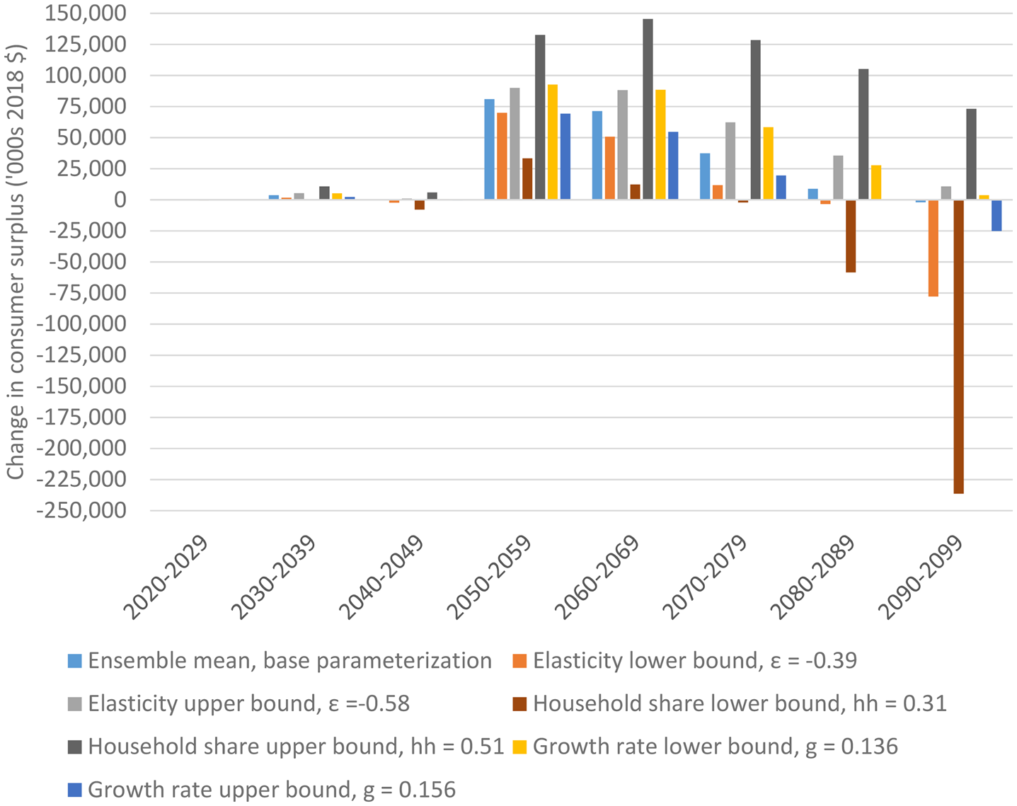
The simple sensitivity tests indicate that the general findings from the ensemble mean projected water volumes are qualitatively similar across alternative model parameters. Given projected water volumes over the century, varying the parameters results in a few shifts from surpluses to shortages in certain decades for the household sector. The largest effect on the change in consumer surplus is the share of water allocated to single family households; using the lower-bound value (31 percent, a 10 percent decrease over the baseline assumption from water-retailer data) results in a large decrease in consumer surplus compared to the baseline. The sensitivity tests also suggest that projections of water volume supplied by the forest (i.e., which climate model is used to generate future water volumes) have a much larger effect on changes in consumer surplus estimates for municipal water. That is, within reasonable assumptions about the demand side of household water, available supply is the primary driver of welfare effects.
Summary
A better understanding of the economic value of water may help planners and policy makers by informing budgetary processes to better reflect resource scarcity and public preferences. Multiple uses for municipal residents, agricultural and industrial purposes, ecological needs such as fish habitat, and recreation, coupled with the projected effects of climate change, will likely exacerbate water shortages in the future, in particular in arid and semi-arid Mediterranean-type areas around the world, such as Southern California (e.g. Giorgi and Lionella Reference Giorgi and Lionello2008). Moreover, the most recent drought in California—from 2011 to 2017—continues to linger in the public's memory, with climate-related precipitation issues continuing to be an ongoing concern for policy makers. Given these stressors to the supply of water in Southern California and challenges associated with climate change, understanding the welfare impacts of changes in the supply of water for downstream users may help forest managers weigh actions that affect water supply and inform water retail agencies’ future investments.
This article estimates projected changes in the value of municipally treated water for household use over the 21st century. The approach relies on comparisons of projected household demand for water to projected available supply from San Bernardino National Forest under numerous potential climate scenarios in each decade. Changes in welfare for single family households are calculated by estimating the change in consumer surplus associated with decreases or increases in consumption necessary to equate the supply of water from the national forest to quantity demanded. Both the household level value and the raw water value are estimated. To the knowledge of the authors, this is the first study to produce such estimates.
The approach employed here describes how consumer welfare changes when climate change affects the supply of water from national forests. When available supply is less than demand, we assume that effective consumption restrictions can be implemented to constrain demand such that consumption equals available supply at projected prices. The foregone consumer surplus associated with a decrease in consumption relative to the quantity demanded represents the value to consumers lost due to inadequate supply from the forest. When supply exceeds quantity demanded, we calculate increases in consumer surplus as if allowing retail prices for water to decrease and consumption to increase until demand equals available supply. The additional surplus that would accrue to consumers under this scenario is interpreted as the potential value to consumers of surplus water from forests.
Results indicate that the ensemble mean climate model projects supply surpluses through the end of the century for the household retail water sector in the study area. These results imply that the average value of an additional unit of raw water provided by San Bernardino National Forest ranges from a low of $0.018 per HCF to $8.37 per HCF through the 21st century (annually in 2018 dollars).
The two additional climate scenarios examined—a warm-wet and a hot-dry scenario—exhibit greater variation in volume of water supplied decade-over-decade. Four of the eight decades project water supply available for households that is less than demanded in the warm-wet scenario, and all eight decades project shortages in the hot-dry scenario. When shortages do occur, the changes in welfare can be substantial.
During the last statewide drought (2011–2017), water retailers became acutely aware of how decreases in water consumption can result in significant, prolonged revenue declines. During this last drought, the State Water Resources Control Board directed water retailers to reexamine their pricing structure (California State Water Resources Control Board, 2018). Since then, most retailers, including all four in this study, now use a tier pricing structure or other type of pricing structure to encourage conservation; additionally, since the drought, many have changed their pricing so as to ensure their rates for the first tier—or lowest level—which has to be paid regardless of consumed volume by the household, is sufficient to cover a significant portion of their fixed costs. In this way, if consumption declines due to a water shortage or the continuing general per capita statewide decline, water retailers will still be able to cover their fixed costs.
Estimates of the value of water supplies provided by national forests may help land managers weigh forest management actions that affect water supply. To the extent that vegetation management, infrastructure investments, and other activities affect the quantity or variability of surface water runoff from forests—and to be clear, the response of surface water runoff to such activities is unknown in many cases—estimates of how consumer surplus changes can help illustrate potential trade-offs of planned activities.
For an illustrative example of how these results could be used, suppose land managers planned vegetation restoration projects over the next decade that, due to increased vegetation cover and evapotranspiration, were expected to decrease expected surface water flows by 250,000 HCF per year over the 2030–2039 decade (about 14.7 percent of the projected surplus from the ensemble mean in that decade). Given the effect on welfare of the supply shortage ($2.01 per HCF based on the ensemble mean), managers could conclude that the benefits of the restoration project must exceed about $500,000, plus the cost of the restoration, to offset welfare losses due to reduced water supply (in 2018 dollars; $2.01/HCF x 250,000 HCF).
The valuation method we describe has several limitations. First, the estimates of changes in consumer surplus rely on integrating the area under a demand function based on price elasticities drawn from the literature that we assume do not change over time. We do not project demand elasticities in the future, and it is unknown how well the existing elasticity estimates will represent demand 20, 30, or 50 years in the future. Moreover, most water utilities in Southern California use tiered pricing strategies (where per-unit rates increase with consumption), which we do not explicitly model here. Relatedly, we do not know what these price structures might look like in the future under different supply scenarios (shortages or surpluses). We have assumed that they will be similar to the current price structures, although future research could examine different price structures, such as water budgets, as a potential response by water retailers to changes in water availability.
Second, we make several assumptions about model parameters that simplify the retail market for water in the study area. We assume that water retailers receive negligible water outside the national forest areas; this assumption aligns with information from the four water retailers included in this study but may be overly restrictive. We also assume that the proportion of retail water delivered to households is fixed at the current average proportion for the four water retailers and that there are negligible demands on water from San Bernardino National Forest outside of the retail water utilities. Basic sensitivity analyses help illustrate how relaxing demand-side assumptions affects estimates; different assumptions about demand-side parameters result in modest changes in consumer surplus estimates. But the future path of the household share of deliveries, or other model parameters, may change in ways that we are not currently able to predict or are outside the range of estimates we explore in the sensitivity tests.
Third, we don't account for nuances in the hydrological system that could affect the timing and size of welfare effects. Storage infrastructure or other investments by water utilities could smooth consumption year-over-year or decade-over-decade. Additionally, we have not incorporated any delay or lag between the provision and availability of water for households. In many parts of California, groundwater is an important—if not the only—source of water. The decadal time steps in the model likely help avoid problems with the timing of groundwater availability. But the model also does not account for changes in the groundwater table—such as wholesalers or retailers pumping water into ground water tables for storage or rehabilitation purposes—that could affect whether municipal pumping of groundwater represents recent infiltration of water from national forests. Incorporating storage and time-lag effects in the model would be useful for future research.
Fourth, we derive at-source value for water from a direct use value for drinking water; indirect use values such as recreation are not considered, nor are other ecosystem functions such as ecological or habitat values. Non-use values such as existence, future option, and bequest values are not considered. As such, the estimates presented here may be interpreted to be lower-bound values.
Finally, we derive the value of water from the single family households served by the retail water sector. Other sectors account for the majority of water deliveries in the study area; understanding demand relationships in these sectors—and in particular how water retailers may respond to changes in demand among sectors (e.g., by encouraging intersectoral trading)—could add to a fuller picture of the effects of changes in water supply from national forests in the future. Furthermore, other demands for water outside of the retail market (such as in-stream flows, agricultural uses in the basin not served by the retailers, or municipal uses in other basins) are not accounted for here.
Water-related ecosystem services are among the most tangible benefits supplied by national forests in Southern California. A future research area could focus on the advantage of coupling the biophysical model outputs with economic water values. Such research can identify spatial heterogeneity in the provision and value of surface water as an ecosystem service. These model projections of water supply vary across space, which when coupled with economic values, may allow policy makers to more comprehensively weigh trade-offs associated with site-specific forest management actions.
Supplementary material
The supplementary material for this article can be found at https://doi.org/10.1017/age.2020.3
Appendix
Projected Change in Temperature and Precipitation from 28 GCMs under RCP8.5 over the 1970–1999 to 2070–2099 Time Period
Results of MC2 Dynamic Vegetation Model
Actual Deliveries and Projected Demands by Water Retailers for Single Family Households and All Retail Sectors, by Year (millions HCF)
Values for Constant kt and Prices (Pt) by decade


 Open access