


1. Introduction
The Evolutionary Map of the Universe (EMU) (Norris et al. Reference Norris2021; Hopkins et al. Reference Hopkins2025) survey is a large-scale radio survey currently being undertaken by the Australian Square Kilometre Array Pathfinder (ASKAP) (Hotan et al. Reference Hotan2021) telescope to map the southern sky at 944 MHz. The improved resolution and sensitivity of modern observatories (e.g. ASKAP, MeerKAT Jonas & MeerKAT Team Reference Jonas2016, etc) allow the discovery and analysis of previously unseen radio objects and emissions. These facilities have revealed numerous new supernova remnants (SNRs) (Filipović et al. Reference Filipović2022, Reference Filipović2023, Reference Filipović2024, Reference Filipović2025b; Sasaki et al. Reference Sasaki2025) and SNR candidates (Smeaton et al. Reference Smeaton2024a, b; Lazarević et al. Reference Lazarević2024a). They have also uncovered several other objects of interest, including pulsar-wind nebulae (PWNe) (Lazarević et al. Reference Lazarević2024b; Ahmad et al. Reference Ahmad2025); reflection nebulae (RNe) (Bradley et al. Reference Bradley2025b); active galactic nuclei (AGNs) (Velović et al. Reference Velović2023; Reference Velović2022); and enigmatic objects of unknown origin (Bordiu et al. Reference Bordiu2024; Smeaton et al. Reference Smeaton2025). ASKAP, alongside other instruments such as MeerKAT, Giant Metrewave Radio Telescope (GMRT) (Ananthakrishnan & Pramesh Rao Reference Ananthakrishnan and Pramesh Rao2001) and Low-Frequency Array (LOFAR) (van Haarlem et al. Reference van Haarlem2013), have also been instrumental to the search for radio counterparts of neutrino detections (Filipović et al. Reference Filipović2025a), as well as the discovery of Odd Radio Circles (ORCs) (Norris et al. Reference Norris2021, Reference Norris2022; Koribalski et al. Reference Koribalski2021; Hota et al. Reference Hota2025; De Gasperin et al. Reference De Gasperin, Brüggen and Pasini2026). These ORCs are an interesting class of new radio objects, appearing exclusively at radio-continuum frequencies. They typically display a circular structure, generally a few arcminutes in size, and often have a central elliptical galaxy visible in the optical, which may be the host of the emission. These properties can vary across different ORCs, however, and the origin of these objects is still being investigated (Norris et al. Reference Norris2021).
One of the most recent EMU survey datasets reveals a patch of diffuse radio emission, EMU J094412 $-$
751016, which we nickname Anglerfish.Footnote
a
This is a distinct extended emission source, composed of an
$-$
751016, which we nickname Anglerfish.Footnote
a
This is a distinct extended emission source, composed of an $\sim 55^{\prime\prime}$
radius circular component, and an
$\sim 55^{\prime\prime}$
radius circular component, and an $\sim30^{\prime\prime}$
extension to the south-east. We find the emission is spatially correlated with two obvious optical and infrared (IR) objects (see Figure 1). We identify the first object as a known IR source WISEA J094409.17
$\sim30^{\prime\prime}$
extension to the south-east. We find the emission is spatially correlated with two obvious optical and infrared (IR) objects (see Figure 1). We identify the first object as a known IR source WISEA J094409.17 $-$
751012.8, and a second object as the semi-variable star V687 Carinae (hereafter referred to as V687 Car).
$-$
751012.8, and a second object as the semi-variable star V687 Carinae (hereafter referred to as V687 Car).
In Section 2 we discuss the data used in this analysis. In Section 3, we present our results. In Section 4, we discuss three main origin scenarios for the radio-continuum emission: (1) a remnant of a stellar mass-loss episode from V687 Car, (2) a high-latitude SNR, and (3) an ORC with WISEA J094409.17 $-$
751012.8 as the host elliptical galaxy. In Section 5, we present our conclusions.
$-$
751012.8 as the host elliptical galaxy. In Section 5, we present our conclusions.
2. Data
ASKAP observed Anglerfish on 25th March 2025 as part of the cEMU survey in tile EMU_0941 $-$
75 (SB72176). The data were reduced using the standard ASKAPSoft data reduction pipeline, which consists of multi-frequency synthesis imaging, multi-scale cleaning, and self-calibration, followed by convolution to a common beam size of B.S.=
$-$
75 (SB72176). The data were reduced using the standard ASKAPSoft data reduction pipeline, which consists of multi-frequency synthesis imaging, multi-scale cleaning, and self-calibration, followed by convolution to a common beam size of B.S.= $15^{\prime\prime}\times15^{\prime\prime}$
(Guzman et al. Reference Guzman2019). The final 944 MHz Stokes I radio image is shown in Figure 1, and we estimate a local RMS noise sensitivity of
$15^{\prime\prime}\times15^{\prime\prime}$
(Guzman et al. Reference Guzman2019). The final 944 MHz Stokes I radio image is shown in Figure 1, and we estimate a local RMS noise sensitivity of $\sim$
25–30
$\sim$
25–30 $\unicode{x03BC}$
Jy beam
$\unicode{x03BC}$
Jy beam $^{-1}$
.
$^{-1}$
.
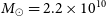
Four-panel image of Anglerfish radio-continuum emission. Top left: 944 MHz ASKAP radio-continuum image (linearly scaled) with a measured Root Mean Squared (RMS) noise level of $\sim$
25–30
$\sim$
25–30 $\unicode{x03BC}$
Jy beam
$\unicode{x03BC}$
Jy beam $^{-1}$
, and a
$^{-1}$
, and a $15^{\prime\prime} \times 15^{\prime\prime}$
convolved beam size shown in the bottom left corner. Contours are from the same image at levels of 60, 100, and 150
$15^{\prime\prime} \times 15^{\prime\prime}$
convolved beam size shown in the bottom left corner. Contours are from the same image at levels of 60, 100, and 150 $\unicode{x03BC}$
Jy beam
$\unicode{x03BC}$
Jy beam $^{-1}$
. Top right: DSS2 IR image. The variable star V687 Car and the elliptical galaxy WISEA J094409.17
$^{-1}$
. Top right: DSS2 IR image. The variable star V687 Car and the elliptical galaxy WISEA J094409.17 $-$
751012.8 are annotated in the image with the solid blue arrows. The dashed orange arrow shows the direction of proper motion of V687 Car. The image is linearly scaled and the contours are from the radio-continuum image at the same levels as the top left panel. Bottom left: Polarised intensity (PI) image with an RMS noise level of 10
$-$
751012.8 are annotated in the image with the solid blue arrows. The dashed orange arrow shows the direction of proper motion of V687 Car. The image is linearly scaled and the contours are from the radio-continuum image at the same levels as the top left panel. Bottom left: Polarised intensity (PI) image with an RMS noise level of 10 $\unicode{x03BC}$
Jy beam
$\unicode{x03BC}$
Jy beam $^{-1}$
. The image is linearly scaled, and the contours are from the radio-continuum image at the same levels as the top left panel. The image is convolved to a beam size of
$^{-1}$
. The image is linearly scaled, and the contours are from the radio-continuum image at the same levels as the top left panel. The image is convolved to a beam size of $18^{\prime\prime}\times 18 ^{\prime\prime}$
, shown in the bottom left corner. There are two point sources in PI at levels of
$18^{\prime\prime}\times 18 ^{\prime\prime}$
, shown in the bottom left corner. There are two point sources in PI at levels of $\sim$
8
$\sim$
8 $\sigma$
and
$\sigma$
and $\sim$
6
$\sim$
6 $\sigma$
, indicated by the blue arrows. Bottom right: RGBY image using radio, optical, and IR data. Red is EMU 944 MHz, green is DSS2 Red, blue is DSS2 blue, and yellow is DSS2 IR. All images are linearly scaled.
$\sigma$
, indicated by the blue arrows. Bottom right: RGBY image using radio, optical, and IR data. Red is EMU 944 MHz, green is DSS2 Red, blue is DSS2 blue, and yellow is DSS2 IR. All images are linearly scaled.

We also use radio polarisation data from the ASKAP Sky Survey of the Universe’s Magnetism (POSSUM) survey (Gaensler et al. Reference Gaensler2025). These data are obtained from the same observations and scheduling blocks as the EMU data. POSSUM data consist of Stokes Q and U polarisation frequency cubes with 1 MHz channels. These images are used to calculate the polarised intensity (PI), and the resulting polarisation images have a lower resolution than EMU (B.S. $= 18^{\prime\prime}\times 18^{\prime\prime}$
; see Figure 1, bottom left).
$= 18^{\prime\prime}\times 18^{\prime\prime}$
; see Figure 1, bottom left).
We use proper motion (PM) measurements obtained from the Gaia telescope (Gaia Collaboration et al. 2016) to determine movements of the star V687 Car. These PM values were obtained from Gaia Data Release 3 (DR3) (Gaia Collaboration et al. 2023a). We also use the distance measurement from Bailer-Jones et al. (Reference Bailer-Jones, Rybizki, Fouesneau, Mantelet and Andrae2018), derived from the Gaia Data Release 2 (DR2) parallax (see Section 4.1).
We use optical data from the Digital Sky Survey 2 (DSS2) optical survey (Lasker et al. Reference Lasker, Software, Systems, Jacoby and Barnes1996), including red, blue, and IR bands to analyse the optical properties of the emission, WISEA J094409.17 $-$
751012.8, and V687 Car (see Figure 1). We also use Wide-Field Infrared Survey Explorer (WISE) (Wright et al. Reference Wright2010) IR observations from Cutri et al. (Reference Cutri2013), specifically the W1 (3.4
$-$
751012.8, and V687 Car (see Figure 1). We also use Wide-Field Infrared Survey Explorer (WISE) (Wright et al. Reference Wright2010) IR observations from Cutri et al. (Reference Cutri2013), specifically the W1 (3.4 $\unicode{x03BC}$
m), W2 (4.6
$\unicode{x03BC}$
m), W2 (4.6 $\unicode{x03BC}$
m), and W3 (12
$\unicode{x03BC}$
m), and W3 (12 $\unicode{x03BC}$
m) bands, to analyse the IR colours of WISEA J094409.17
$\unicode{x03BC}$
m) bands, to analyse the IR colours of WISEA J094409.17 $-$
751012.8.
$-$
751012.8.
Finally, we searched for any sign of Anglerfish at other frequencies but found no corresponding emission. Specifically, we searched in FIR (Spitzer), UV (GALEX), X-ray (RASS, eRASS DR1, XMM-Newton, and Chandra), and $\gamma$
-ray (Fermi). Other available radio surveys, including the Rapid ASKAP Continuum Survey (RACS) (McConnell et al. Reference McConnell2020), University Molonglo Sky Survey (SUMSS) (Mauch et al. Reference Mauch2003) and Parkes-MIT-NRAO (PMN) (Wright et al. Reference Wright1996) were also searched, but no traces of emission associated with Anglerfish were found.
$\gamma$
-ray (Fermi). Other available radio surveys, including the Rapid ASKAP Continuum Survey (RACS) (McConnell et al. Reference McConnell2020), University Molonglo Sky Survey (SUMSS) (Mauch et al. Reference Mauch2003) and Parkes-MIT-NRAO (PMN) (Wright et al. Reference Wright1996) were also searched, but no traces of emission associated with Anglerfish were found.
3. Results
The Anglerfish radio emission has two distinct components (Figure 1); a circular region centred at $\mathrm{RA(J2000)} = 09^\mathrm{h} 44^\mathrm{m}12.3^\mathrm{s}$
, Dec(J2000) =
$\mathrm{RA(J2000)} = 09^\mathrm{h} 44^\mathrm{m}12.3^\mathrm{s}$
, Dec(J2000) = $- 75^\circ 10^\prime 16 .\!\!^{\prime\prime}9$
(Galactic coordinates:
$- 75^\circ 10^\prime 16 .\!\!^{\prime\prime}9$
(Galactic coordinates: $l = 291.7^\circ$
, b =
$l = 291.7^\circ$
, b = $-$
16.5
$-$
16.5 $^\circ$
) with radius
$^\circ$
) with radius $\sim55^{\prime\prime}$
, and a region which extends
$\sim55^{\prime\prime}$
, and a region which extends $\sim 30^{\prime\prime}$
towards the south-east. The entire area is elliptical, centred at
$\sim 30^{\prime\prime}$
towards the south-east. The entire area is elliptical, centred at $\mathrm{RA(J2000)} = 09^\mathrm{h} 44^\mathrm{m} 18.6 ^\mathrm{s}$
,
$\mathrm{RA(J2000)} = 09^\mathrm{h} 44^\mathrm{m} 18.6 ^\mathrm{s}$
, $\mathrm{Dec(J2000)} = -75^\circ 10' 26 .\!^{\prime\prime} 7$
(angled at 22 degrees) with semi-axes of
$\mathrm{Dec(J2000)} = -75^\circ 10' 26 .\!^{\prime\prime} 7$
(angled at 22 degrees) with semi-axes of $60^{\prime\prime}$
and
$60^{\prime\prime}$
and $90^{\prime\prime}$
, which is shown in Figure 4. There are no obvious radio point sources visible within the emission.
$90^{\prime\prime}$
, which is shown in Figure 4. There are no obvious radio point sources visible within the emission.
We analysed the Stokes V EMU data, but detected no circular polarisation. We follow a process similar to that used in Filipović et al. (Reference Filipović2025a), using the POSSUM data to create Faraday spectra and calculate the PI of Anglerfish. We then calculate the rotation measure of the polarisation, using the rotation measure synthesis technique (see Burn Reference Burn1966; Brentjens & de Bruyn Reference Brentjens and de Bruyn2005 or additionally Harvey-Smith et al. Reference Harvey-Smith2010) as detailed in Ball et al. (Reference Ball2023), to de-rotate the linear polarisations. The detailed polarisation images are shown in Figure 1, and the PI image achieves an RMS noise level of 10 $\unicode{x03BC}$
Jy beam
$\unicode{x03BC}$
Jy beam $^{-1}$
, which is taken from the Faraday depth spectra. The peak in PI is 83
$^{-1}$
, which is taken from the Faraday depth spectra. The peak in PI is 83 $\unicode{x03BC}$
Jy beam
$\unicode{x03BC}$
Jy beam $^{-1}$
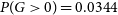
, as can be seen in Figure 2 while in total power, we measure 110
$^{-1}$
, as can be seen in Figure 2 while in total power, we measure 110 $\unicode{x03BC}$
Jy beam
$\unicode{x03BC}$
Jy beam $^{-1}$
in the same location. That gives 75% of fractional polarisation, which is acceptable, given the above uncertainties.
$^{-1}$
in the same location. That gives 75% of fractional polarisation, which is acceptable, given the above uncertainties.
Faraday Depth Spectrum of the brightest peak in the PI map displayed in Figure 1, where it is indicated by the left blue arrow. In the top right inset, we show an inset zooming in on the peak, indicating a non-zero RM.

We observed two areas of polarisation emission, with peaks of 60 and 80 $\unicode{x03BC}$
Jy, giving significance levels of 6 and 8
$\unicode{x03BC}$
Jy, giving significance levels of 6 and 8 $\sigma$
, respectively (see Figures 1 and 2). It should be noted that the noise in the Faraday depth spectra is Ricean, not Gaussian, and we have therefore adopted an 8
$\sigma$
, respectively (see Figures 1 and 2). It should be noted that the noise in the Faraday depth spectra is Ricean, not Gaussian, and we have therefore adopted an 8 $\sigma$
detection threshold. This 8
$\sigma$
detection threshold. This 8 $\sigma$
threshold approximately corresponds to a false positive rate of
$\sigma$
threshold approximately corresponds to a false positive rate of $\sim$
4% (George, Stil, & Keller Reference George, Stil and Keller2012). Therefore, we take the 8
$\sim$
4% (George, Stil, & Keller Reference George, Stil and Keller2012). Therefore, we take the 8 $\sigma$
peak as a detection and the 6
$\sigma$
peak as a detection and the 6 $\sigma$
peak as a marginal detection. These regions are located on the edge of the Anglerfish’s emission, but do not spatially coincide with the brightest Stokes I emission. These faint polarised sources are consistent with polarisation arising from shell expansion. If the emission is of synchrotron origin, then this would require coincident magnetic fields. Thus, the fact that the polarisation peaks are anti-correlated with the Stokes I total intensity implies that depolarisation may be taking place, in the case of non-thermal emission. This would likely be due to denser or more magnetised media associated with the peak positions of the total intensity. The thermal vs. non-thermal nature of the radio emission is unclear, but the current data suggest non-thermal emission is more likely, as discussed later in this section. The 8
$\sigma$
peak as a marginal detection. These regions are located on the edge of the Anglerfish’s emission, but do not spatially coincide with the brightest Stokes I emission. These faint polarised sources are consistent with polarisation arising from shell expansion. If the emission is of synchrotron origin, then this would require coincident magnetic fields. Thus, the fact that the polarisation peaks are anti-correlated with the Stokes I total intensity implies that depolarisation may be taking place, in the case of non-thermal emission. This would likely be due to denser or more magnetised media associated with the peak positions of the total intensity. The thermal vs. non-thermal nature of the radio emission is unclear, but the current data suggest non-thermal emission is more likely, as discussed later in this section. The 8 $\sigma$
peak to the left in Figure 1 is considered significant at the detection threshold (see Figure 2), however, as it is a point-like source, it could be the polarised emission of an unrelated background source. We find that the polarisation results are fairly weak, and thus determine that they should not be relied on for further theoretical analysis.
$\sigma$
peak to the left in Figure 1 is considered significant at the detection threshold (see Figure 2), however, as it is a point-like source, it could be the polarised emission of an unrelated background source. We find that the polarisation results are fairly weak, and thus determine that they should not be relied on for further theoretical analysis.
We use the elliptical region defined above to measure the flux density of Anglerfish using the astronomy software Cube Analysis and Rendering Tool for Astronomy (CARTA) (Comrie et al. Reference Comrie2018). We subtract the nearby diffuse background flux density, following the process of Hurley-Walker et al. (Reference Hurley-Walker2019), and assume a 10% error, following the process of Filipović et al. (Reference Filipović2022). We note that Anglerfish is located away from the Galactic Plane (b = $-$
16.5
$-$
16.5 $^\circ$
) and therefore the contribution of this background noise is minimal. We measure an integrated radio flux density of Anglerfish to be
$^\circ$
) and therefore the contribution of this background noise is minimal. We measure an integrated radio flux density of Anglerfish to be $S_{943\,\rm MHz}=5.0\pm 0.5$
mJy. We assume a 10% uncertainty due to the object’s faintness, similar to the methods used in other analyses of low-surface-brightness, diffuse radio objects (Filipović et al. Reference Filipović2022; Smeaton et al. Reference Smeaton2025). As we have no other detections at radio frequencies, we cannot determine the radio spectral index. We attempted to use the ASKAP Taylor 1 (T1) image to estimate the ASKAP in-band spectral index. However, given the low surface brightness, the results are unrealistic and have very large errors. Therefore, we instead use the available GaLactic and Extragalactic All-sky MWA Survey (GLEAM) 200 MHz radio data from the MurchisonWidefield Array (MWA) telescope (Hurley-Walker et al. Reference Hurley-Walker2017) and 1367 MHz RACS data from the ASKAP telescope (McConnell et al. Reference McConnell2020) to estimate limits on the spectral index. We do not detect Anglerfish in either survey, so these upper flux density limits provide a possible spectral index range.
$S_{943\,\rm MHz}=5.0\pm 0.5$
mJy. We assume a 10% uncertainty due to the object’s faintness, similar to the methods used in other analyses of low-surface-brightness, diffuse radio objects (Filipović et al. Reference Filipović2022; Smeaton et al. Reference Smeaton2025). As we have no other detections at radio frequencies, we cannot determine the radio spectral index. We attempted to use the ASKAP Taylor 1 (T1) image to estimate the ASKAP in-band spectral index. However, given the low surface brightness, the results are unrealistic and have very large errors. Therefore, we instead use the available GaLactic and Extragalactic All-sky MWA Survey (GLEAM) 200 MHz radio data from the MurchisonWidefield Array (MWA) telescope (Hurley-Walker et al. Reference Hurley-Walker2017) and 1367 MHz RACS data from the ASKAP telescope (McConnell et al. Reference McConnell2020) to estimate limits on the spectral index. We do not detect Anglerfish in either survey, so these upper flux density limits provide a possible spectral index range.
Anglerfish would appear as an extended object in the RACS data and as a point source in the MWA data, thus the limits are calculated slightly differently. Measuring an upper limit of a non-detection can be sensitive to the noise level used, and so a more robust method is chosen for the RACS and MWA noise levels. We measured the local RMS noise by generating a histogram of pixel values within a region surrounding the Anglerfish location and fitting a Gaussian to the negative pixel values, taking the measured $\sigma$
as the uncertainty (see Figure A1). This approach avoids contamination from positive source emission and ensures only the local noise is measured. This resulted in values of 0.24 mJy for RACS and 9.75 mJy for MWA.
$\sigma$
as the uncertainty (see Figure A1). This approach avoids contamination from positive source emission and ensures only the local noise is measured. This resulted in values of 0.24 mJy for RACS and 9.75 mJy for MWA.
To estimate the upper limit for a non-detection of an extended object, we estimate the uncertainty (noise level) over the source area and multiply this by 3 for a 3 $\sigma$
detection limit. We use the elliptical region of
$\sigma$
detection limit. We use the elliptical region of $60^{\prime\prime}\times 90^{\prime\prime}$
for the source area,
$60^{\prime\prime}\times 90^{\prime\prime}$
for the source area, $\Omega_\mathrm{source}$
, and the RACS beam size of
$\Omega_\mathrm{source}$
, and the RACS beam size of $13.1^{\prime\prime}\times 9.3^{\prime\prime}$
to calculate the number of beams covering the source as
$13.1^{\prime\prime}\times 9.3^{\prime\prime}$
to calculate the number of beams covering the source as $N = \Omega_\mathrm{ source}/\Omega_{\rm beam}$
. Each of these beams has an RMS noise level of
$N = \Omega_\mathrm{ source}/\Omega_{\rm beam}$
. Each of these beams has an RMS noise level of $\sigma_\mathrm{rms}$
which we estimate as 0.24 mJy beam
$\sigma_\mathrm{rms}$
which we estimate as 0.24 mJy beam $^{-1}$
(Figure A1, left). We assume that the noise in each beam is uncorrelated and thus independent of each other, and so the total uncertainty follows error propagation for N independent measurements with the same uncertainty
$^{-1}$
(Figure A1, left). We assume that the noise in each beam is uncorrelated and thus independent of each other, and so the total uncertainty follows error propagation for N independent measurements with the same uncertainty $\sigma_\mathrm{rms}$
, which gives
$\sigma_\mathrm{rms}$
, which gives $\sigma_\mathrm{total}$
=
$\sigma_\mathrm{total}$
= $\sigma_\mathrm{rms}\times\sqrt{N}$
. Therefore, for a 3
$\sigma_\mathrm{rms}\times\sqrt{N}$
. Therefore, for a 3 $\sigma$
detection limit, the upper RACS 1 367 MHz flux density limit is calculated as
$\sigma$
detection limit, the upper RACS 1 367 MHz flux density limit is calculated as $S \lt 3\times\sigma_\mathrm{rms}\times\sqrt{\Omega_\mathrm{source}/\Omega_\mathrm{ beam}}$
= 4.8 mJy.
$S \lt 3\times\sigma_\mathrm{rms}\times\sqrt{\Omega_\mathrm{source}/\Omega_\mathrm{ beam}}$
= 4.8 mJy.
The method used for this limit estimation assumes that the individual beams are uncorrelated. For radio interferometric imaging, the image pixels are inherently correlated to an extent due to the Fourier transform process. However, for extended sources which cover multiple beams (in our case, Anglerfish covers $\Omega_\mathrm{source}/\Omega_\mathrm{beam}\sim44$
beams), this correlation is typically not significant. To test the impact of potential beam-correlation effects, we independently calculate an upper limit using an empirical approach that inherently accounts for pixel correlations in the data. For this, we generate 25 apertures of the source size (
$\Omega_\mathrm{source}/\Omega_\mathrm{beam}\sim44$
beams), this correlation is typically not significant. To test the impact of potential beam-correlation effects, we independently calculate an upper limit using an empirical approach that inherently accounts for pixel correlations in the data. For this, we generate 25 apertures of the source size ( $60^{\prime\prime}\times 90^{\prime\prime}$
) distributed on the RACS image in blank sky surrounding the source. We measure the integrated flux density for each of these apertures and calculate the standard deviation, which gives a value of 1.38 mJy. Assuming a 3
$60^{\prime\prime}\times 90^{\prime\prime}$
) distributed on the RACS image in blank sky surrounding the source. We measure the integrated flux density for each of these apertures and calculate the standard deviation, which gives a value of 1.38 mJy. Assuming a 3 $\sigma$
detection threshold, this gives an upper limit of 4.1 mJy. This is slightly lower than the previously calculated 4.8 mJy (within 16%) and shows that these correlation effects are not significantly biasing the results. We adopt the more conservative value of 4.8 mJy as the 1 367 MHz flux density RACS upper limit for the subsequent analysis.
$\sigma$
detection threshold, this gives an upper limit of 4.1 mJy. This is slightly lower than the previously calculated 4.8 mJy (within 16%) and shows that these correlation effects are not significantly biasing the results. We adopt the more conservative value of 4.8 mJy as the 1 367 MHz flux density RACS upper limit for the subsequent analysis.
For the MWA image, as the source would appear as a point source were it detectable, the estimation is simpler and the source area is taken to be equivalent to the beam area. Therefore, the above equation simplifies to an upper limit of $S\lt3\sigma$
, where
$S\lt3\sigma$
, where $\sigma$
is the measured local RMS noise which we measure as
$\sigma$
is the measured local RMS noise which we measure as $\sim$
9.75 mJy beam
$\sim$
9.75 mJy beam $^{-1}$
(Figure A1, right). Therefore, the MWA 200 MHz upper limit is taken as
$^{-1}$
(Figure A1, right). Therefore, the MWA 200 MHz upper limit is taken as $\sim$
29.3 mJy.
$\sim$
29.3 mJy.
Using the measured 944 MHz point and the two upper limit flux densities, we calculate a possible spectral index range for the emission. This is done by generating two linear fits as the boundaries of this range, one being through the 944 MHz EMU point and the RACS upper limit, and the other through the EMU point and the MWA upper limit (see Figure 3). We calculate the uncertainties in these limits by also calculating the lines of worst fit through the EMU upper and lower uncertainties ( $5.0\pm 0.5$
mJy). These spectral index uncertainties are shown as the shaded blue regions in Figure 3. This gives a shallow limit of
$5.0\pm 0.5$
mJy). These spectral index uncertainties are shown as the shaded blue regions in Figure 3. This gives a shallow limit of $\alpha = -0.1\pm0.3$
and a steep limit of
$\alpha = -0.1\pm0.3$
and a steep limit of $\alpha = -1.2\pm0.1$
. The data are not sufficient to constrain the spectral index any further, and this entire range (the hashed region in Figure 3 of
$\alpha = -1.2\pm0.1$
. The data are not sufficient to constrain the spectral index any further, and this entire range (the hashed region in Figure 3 of $-1.3\lt\alpha\lt0.2$
) is the possible spectral index range from the given uncertainties. Both flat and steep spectral indices are thus consistent with the current data, and so both thermal and non-thermal mechanisms are possible. For radio spectral indices, a reasonable cut-off between thermal and non-thermal emission can be assumed to be
$-1.3\lt\alpha\lt0.2$
) is the possible spectral index range from the given uncertainties. Both flat and steep spectral indices are thus consistent with the current data, and so both thermal and non-thermal mechanisms are possible. For radio spectral indices, a reasonable cut-off between thermal and non-thermal emission can be assumed to be $-0.3$
, with steeper values likely indicating non-thermal, synchrotron emission. Taking
$-0.3$
, with steeper values likely indicating non-thermal, synchrotron emission. Taking $\alpha=-0.3$
as a general dividing line, this shows that two-thirds of the entire uncertainty range is within the non-thermal regime (
$\alpha=-0.3$
as a general dividing line, this shows that two-thirds of the entire uncertainty range is within the non-thermal regime ( $\alpha\lt-0.3$
) and one-third is flatter (
$\alpha\lt-0.3$
) and one-third is flatter ( $\alpha\gt-0.3$
). Therefore, with no other data available, we conclude a non-thermal spectral index is more likely from this range, but emphasise that it cannot be properly constrained without more data. The current data do not allow us to test the possibilities of any more complex spectral shapes, and a linear fit is assumed. If the spectral index is indeed non-thermal, this would support the SNR and ORC scenarios described in Sections 4.2 and 4.3. Conversely, a flatter spectral index instead supports the stellar outburst scenario described in Section 4.1.
$\alpha\gt-0.3$
). Therefore, with no other data available, we conclude a non-thermal spectral index is more likely from this range, but emphasise that it cannot be properly constrained without more data. The current data do not allow us to test the possibilities of any more complex spectral shapes, and a linear fit is assumed. If the spectral index is indeed non-thermal, this would support the SNR and ORC scenarios described in Sections 4.2 and 4.3. Conversely, a flatter spectral index instead supports the stellar outburst scenario described in Section 4.1.
Spectral index graph of the Anglerfish emission, using the flux density measurement from the EMU data, and the upper limits from the RACS and GLEAM data to generate shallow (dotted line) and steep (dashed line) limits for the spectral index. The uncertainty ranges for each of these spectral index fits is shown as a shaded blue region around each line. The hashed area in between represents the possible spectral index range.

We find that Anglerfish emits exclusively at radio frequencies, as demonstrated by the lack of detection at other frequencies across multiple surveys (listed at the end of Section 2). We searched for potential counterparts for this emission in the Hong Kong/AAO/Strasbourg H $\alpha$
(HASH) Planetary Nebula (PN) catalogue (Parker, Bojicčić, & Frew Reference Parker, Bojičić and Frew2016), and the Galactic SNR catalogue of Green (Reference Green2025), but found no corresponding sources. We therefore investigate the two distinctive, centrally positioned optical sources (see Figure 1) as prime candidates for the origin of this radio-continuum emission. The yellowish source on the left is the semi-variable star V687 Car, and the white right-hand point source is the elliptical galaxy WISEA J094409.17
$\alpha$
(HASH) Planetary Nebula (PN) catalogue (Parker, Bojicčić, & Frew Reference Parker, Bojičić and Frew2016), and the Galactic SNR catalogue of Green (Reference Green2025), but found no corresponding sources. We therefore investigate the two distinctive, centrally positioned optical sources (see Figure 1) as prime candidates for the origin of this radio-continuum emission. The yellowish source on the left is the semi-variable star V687 Car, and the white right-hand point source is the elliptical galaxy WISEA J094409.17 $-$
751012.8.
$-$
751012.8.
4. Discussion
4.1. Anglerfish as stellar (V687 Car) mass-loss episode
V687 Car (also referred to as IRAS 09440 $-$
7456) is a semi-regular variable star first identified by Bedient (Reference Bedient2007). The online SIMBAD database lists V687 Car as a Mira Ceti type variable, for which it references (Samus et al. Reference Samus, Kazarovets, Durlevich, Kireeva and Pastukhova2009). However, this entry does not list the star as a Mira Ceti type variable. Subsequent observations have confirmed its variability to be semi-variable type A (Samus et al. Reference Samus, Kazarovets, Durlevich, Kireeva and Pastukhova2017). Despite the star’s known variability, there is no clear indication of its spectral classification. Gaia DR3 (Gaia Collaboration et al. 2023a) lists an effective temperature of 3 285.7 K and an absolute magnitude in the G band of
$-$
7456) is a semi-regular variable star first identified by Bedient (Reference Bedient2007). The online SIMBAD database lists V687 Car as a Mira Ceti type variable, for which it references (Samus et al. Reference Samus, Kazarovets, Durlevich, Kireeva and Pastukhova2009). However, this entry does not list the star as a Mira Ceti type variable. Subsequent observations have confirmed its variability to be semi-variable type A (Samus et al. Reference Samus, Kazarovets, Durlevich, Kireeva and Pastukhova2017). Despite the star’s known variability, there is no clear indication of its spectral classification. Gaia DR3 (Gaia Collaboration et al. 2023a) lists an effective temperature of 3 285.7 K and an absolute magnitude in the G band of $-1.33$
. Tracing these values on the Hertzsprung-Russell diagram (Filipović & Tothill Reference Filipović and Tothill2021) indicates that V687 Car is an M-Type giant.
$-1.33$
. Tracing these values on the Hertzsprung-Russell diagram (Filipović & Tothill Reference Filipović and Tothill2021) indicates that V687 Car is an M-Type giant.
Semi-regular variable stars are evolved giants with intermediate to late spectral types (M, C, S, etc. Lundgren Reference Lundgren1988). They typically exhibit brightness variations with periods ranging from $\sim$
35 to 1 200 d, which can be interspersed by irregular behaviour. Unlike Mira variables, which display large amplitude brightness variations, semi-regular type A stars have smaller amplitude changes (
$\sim$
35 to 1 200 d, which can be interspersed by irregular behaviour. Unlike Mira variables, which display large amplitude brightness variations, semi-regular type A stars have smaller amplitude changes ( $\lt$
2.5 mag; Trabucchi, Mowlavi, & Lebzelter Reference Trabucchi, Mowlavi and Lebzelter2021). V687 Car’s variability is measured as fluctuating between apparent V-band magnitudes of
$\lt$
2.5 mag; Trabucchi, Mowlavi, & Lebzelter Reference Trabucchi, Mowlavi and Lebzelter2021). V687 Car’s variability is measured as fluctuating between apparent V-band magnitudes of $\sim$
13–14.5 with a period of 240 d (Bedient Reference Bedient2007), as expected for semi-regular type A stars. These stars can undergo significant mass-loss (Cranmer & Saar Reference Cranmer and Saar2011), resulting in weak thermal free-free radio emission from ionised winds or circumstellar envelopes, and in some cases, from molecular maser emission (McIntosh & Indermuehle Reference McIntosh and Indermuehle2015). Bailer-Jones et al. (Reference Bailer-Jones, Rybizki, Fouesneau, Demleitner and Andrae2021) estimated a distance to V687 Car of
$\sim$
13–14.5 with a period of 240 d (Bedient Reference Bedient2007), as expected for semi-regular type A stars. These stars can undergo significant mass-loss (Cranmer & Saar Reference Cranmer and Saar2011), resulting in weak thermal free-free radio emission from ionised winds or circumstellar envelopes, and in some cases, from molecular maser emission (McIntosh & Indermuehle Reference McIntosh and Indermuehle2015). Bailer-Jones et al. (Reference Bailer-Jones, Rybizki, Fouesneau, Demleitner and Andrae2021) estimated a distance to V687 Car of $2.08^{+0.29}_{-0.22}$
kpc, and if we place the radio–continuum feature at this distance, its size would be
$2.08^{+0.29}_{-0.22}$
kpc, and if we place the radio–continuum feature at this distance, its size would be $\sim$
1.21
$\sim$
1.21 $\times$
1.82 pc (based on the elliptical region defined in Section 3).
$\times$
1.82 pc (based on the elliptical region defined in Section 3).
ASKAP EMU 944 MHz image of the Anglerfish radio emission with superimposed measurements used in Section 4.1. The image is linearly scaled with the beam size shown in the bottom left corner. The black circle denotes the elliptical region defined in Section 3. The white dashed line represents V687 Car’s tangential movement, with two arrows indicating its direction. The green square shows the location of V687 Car, the white ‘X’ shows the geometric centre of the emission (discussed in Section 3, and the red circle denotes V687 Car’s closest approach to the geometric centre.

V687 Car has FK5 PM of $\mu_{\alpha}$
:
$\mu_{\alpha}$
: $-6.877\pm 0.066$
mas yr
$-6.877\pm 0.066$
mas yr $^{-1}$
and
$^{-1}$
and $\mu_{\delta}$
:
$\mu_{\delta}$
: $5.374\pm 0.065$
mas yr
$5.374\pm 0.065$
mas yr $^{-1}$
. To account for peculiar velocity, we first converted the FK5 PM to Galactic Coordinates;
$^{-1}$
. To account for peculiar velocity, we first converted the FK5 PM to Galactic Coordinates; $\mu_{l}$
:
$\mu_{l}$
: $-8.699\pm 0.087$
mas yr
$-8.699\pm 0.087$
mas yr $^{-1}$
and
$^{-1}$
and $\mu_{b}$
:
$\mu_{b}$
: $-0.697\pm 0.069$
mas yr
$-0.697\pm 0.069$
mas yr $^{-1}$
. Then, using the equations discussed by (Comerón & Pasquali Reference Comerón and Pasquali2007, Equations; 2a, 2b, 3a, and 3b), we derive peculiar PMs of V687 Car;
$^{-1}$
. Then, using the equations discussed by (Comerón & Pasquali Reference Comerón and Pasquali2007, Equations; 2a, 2b, 3a, and 3b), we derive peculiar PMs of V687 Car; $\mu_{l}$
:
$\mu_{l}$
: $-3.149\pm 0.087$
mas yr
$-3.149\pm 0.087$
mas yr $^{-1}$
and
$^{-1}$
and $\mu_{b}$
:
$\mu_{b}$
: $0.178\pm 0.069$
mas yr
$0.178\pm 0.069$
mas yr $^{-1}$
. These correspond to peculiar velocities of 31.1
$^{-1}$
. These correspond to peculiar velocities of 31.1 $\pm$
0.9 km s
$\pm$
0.9 km s $^{-1}$
and 1.8
$^{-1}$
and 1.8 $\pm$
0.7 km s
$\pm$
0.7 km s $^{-1}$
, and a tangential peculiar velocity of 31.2
$^{-1}$
, and a tangential peculiar velocity of 31.2 $\pm$
0.8 km s
$\pm$
0.8 km s $^{-1}$
. The movement of V687 Car is shown in Figure 1 (top–right) and Figure 4, with the star shown to be moving in a north-westerly direction, aligned with the head-tail radio structure observed in the larger emission.
$^{-1}$
. The movement of V687 Car is shown in Figure 1 (top–right) and Figure 4, with the star shown to be moving in a north-westerly direction, aligned with the head-tail radio structure observed in the larger emission.
The projected PM of V687 Car somewhat matches the geometry of the irregular elliptical shape of the radio–continuum emission, although the peculiar velocity indicates that it is moving more northern than north-westerly (See Figure 4). As it is possible that this is a chance alignment, we estimate the probability of a chance alignment using the Gaia DR3 data. The probability of one or more stars with magnitude equivalent or brighter than V687 Car appearing in the Anglerfish emission area is given as $P(S\gt0)$
, where P is the Poisson distribution with rate
$P(S\gt0)$
, where P is the Poisson distribution with rate $\lambda$
, where
$\lambda$
, where $\lambda$
is the expected number of stars. We use the Gaia DR3 G-band magnitude of 10.28, for this estimate. We note this magnitude is higher than the previous V-band magnitude of Bedient (Reference Bedient2007), possibly due to the different bandwidth. As this value is from the Gaia catalogue, we use this for the probability calculation to ensure consistent cross-matching between the catalogue. We estimate the rate by measuring the number of candidate stars in a search area of radius
$\lambda$
is the expected number of stars. We use the Gaia DR3 G-band magnitude of 10.28, for this estimate. We note this magnitude is higher than the previous V-band magnitude of Bedient (Reference Bedient2007), possibly due to the different bandwidth. As this value is from the Gaia catalogue, we use this for the probability calculation to ensure consistent cross-matching between the catalogue. We estimate the rate by measuring the number of candidate stars in a search area of radius $60^\prime$
, with an area
$60^\prime$
, with an area $\pi\times60^2 = 11\,309.73$
square arcminutes. 79 stars satisfying the criteria were found, giving a rate of
$\pi\times60^2 = 11\,309.73$
square arcminutes. 79 stars satisfying the criteria were found, giving a rate of $79/11\,309.73 = 0.0069$
stars per square arcminute. Using the Anglerfish elliptical area defined earlier as 4.72 square arcminutes, the expected rate is
$79/11\,309.73 = 0.0069$
stars per square arcminute. Using the Anglerfish elliptical area defined earlier as 4.72 square arcminutes, the expected rate is $\lambda=0.0069\times4.72 = 0.033$
stars per 4.72 square arcminutes. Therefore, the probability of one or more stars appearing in the region, independent of Anglerfish, is estimated as
$\lambda=0.0069\times4.72 = 0.033$
stars per 4.72 square arcminutes. Therefore, the probability of one or more stars appearing in the region, independent of Anglerfish, is estimated as $P(S\gt0) = 0.0325$
using the Poisson distribution. This is indicative of a low probability of chance alignment.
$P(S\gt0) = 0.0325$
using the Poisson distribution. This is indicative of a low probability of chance alignment.
Using a method similar to that explored by Bradley et al. (Reference Bradley2025a), we can calculate V687 Car’s trajectory and determine a theoretical age and expansion velocity for the supposed mass-loss shell. Figure 4 shows measurements of the star’s projected motion across the radio–continuum emission. Assuming that the centre of the ellipse used to measure the radio–continuum emission (see Section 3) is close to the geometric centre of the shell, the point at which V687 Car comes closest to the centre of the emission is RA(J2000) $=$
09
$=$
09 $^\mathrm{h}$
44
$^\mathrm{h}$
44 $^\mathrm{m}$
19.34
$^\mathrm{m}$
19.34 $^\mathrm{s}$
, Dec(J2000)
$^\mathrm{s}$
, Dec(J2000) $=-$
75
$=-$
75 $^\circ$
10’24.23”. The angular distance from V687 Car to the ‘centre’ coordinates is
$^\circ$
10’24.23”. The angular distance from V687 Car to the ‘centre’ coordinates is $\sim$
16
$\sim$
16 $^{\prime\prime}$
, and using the same method in Bradley et al. (Reference Bradley2025a), we determine the time travelled to be
$^{\prime\prime}$
, and using the same method in Bradley et al. (Reference Bradley2025a), we determine the time travelled to be $5\,060\pm 130$
yr. Assuming the mass-loss shell originated at this point, we take the calculated time as an estimate of the shell’s age. Measuring the longest distance of the travelled emission (90
$5\,060\pm 130$
yr. Assuming the mass-loss shell originated at this point, we take the calculated time as an estimate of the shell’s age. Measuring the longest distance of the travelled emission (90 $^{\prime\prime}$
, from the elliptical region), and dividing by the shell age, we determine an average expansion velocity of
$^{\prime\prime}$
, from the elliptical region), and dividing by the shell age, we determine an average expansion velocity of $175\pm 5$
km s
$175\pm 5$
km s $^{-1}$
. It is important to note that this assumes the radio-continuum emission began at its apparent centre and a 2-dimensional plane, making the age estimate a lower limit and the expansion velocity estimate an upper limit.
$^{-1}$
. It is important to note that this assumes the radio-continuum emission began at its apparent centre and a 2-dimensional plane, making the age estimate a lower limit and the expansion velocity estimate an upper limit.
Considering our calculated average expansion velocity of $175\pm 5$
km s
$175\pm 5$
km s $^{-1}$
, it is important to note that the expected stellar wind velocity of an M-type giant does not typically exceed
$^{-1}$
, it is important to note that the expected stellar wind velocity of an M-type giant does not typically exceed $\sim$
20 km s
$\sim$
20 km s $^{-1}$
(Bladh et al. Reference Bladh, Höfner, Aringer and Eriksson2015; Liljegren et al. Reference Liljegren, Höfner, Eriksson and Nowotny2017). This makes V687 Car an unlikely host for the radio emission, as the stellar wind output is not powerful enough to sustain a shell of this size. The spectral index range calculated suggests that the radio emission is consistent with both thermal and non-thermal origins (see Section 3). The mass-loss episode scenario would be expected to generate thermal emission, which is consistent with the spectral index range.
$^{-1}$
(Bladh et al. Reference Bladh, Höfner, Aringer and Eriksson2015; Liljegren et al. Reference Liljegren, Höfner, Eriksson and Nowotny2017). This makes V687 Car an unlikely host for the radio emission, as the stellar wind output is not powerful enough to sustain a shell of this size. The spectral index range calculated suggests that the radio emission is consistent with both thermal and non-thermal origins (see Section 3). The mass-loss episode scenario would be expected to generate thermal emission, which is consistent with the spectral index range.
4.2. Anglerfish as a high latitude supernova remnant
We also consider the possibility that Anglerfish may be a high-latitude SNR, similar to ones such as Calvera (Arias et al. Reference Arias2022), G70.0 $-$
21.5 (Fesen et al. Reference Fesen, Neustadt, Black and Koeppel2015), and G181.1+9.5 (Kothes et al. Reference Kothes, Reich, Foster and Reich2017). The expected spectral index of an SNR is
$-$
21.5 (Fesen et al. Reference Fesen, Neustadt, Black and Koeppel2015), and G181.1+9.5 (Kothes et al. Reference Kothes, Reich, Foster and Reich2017). The expected spectral index of an SNR is $\sim-0.5$
(Galactic average is
$\sim-0.5$
(Galactic average is $-$
0.51
$-$
0.51 $\pm$
0.01 Ranasinghe & Leahy Reference Ranasinghe and Leahy2023), which is within the spectral index range given in Section 3. The spectral index is only weakly constrained, however, and other physical properties act as a more accurate indicator of the Anglerfish’s nature. At Anglerfish’s direction (l = 291.7
$\pm$
0.01 Ranasinghe & Leahy Reference Ranasinghe and Leahy2023), which is within the spectral index range given in Section 3. The spectral index is only weakly constrained, however, and other physical properties act as a more accurate indicator of the Anglerfish’s nature. At Anglerfish’s direction (l = 291.7 $^\circ$
, b =
$^\circ$
, b = $-$
16.5
$-$
16.5 $^\circ$
), we can calculate a maximum distance if we assume that it would be located within the Galactic disk. Assuming a maximum disk width of
$^\circ$
), we can calculate a maximum distance if we assume that it would be located within the Galactic disk. Assuming a maximum disk width of $\sim$
1 kpc we estimate a maximum likely distance of
$\sim$
1 kpc we estimate a maximum likely distance of $D=1\textrm{~kpc}/\textrm{sin}(\!-16.5$ $^\circ$ $)=\,\sim3.5$
kpc, corresponding to a physical diameter of
$)=\,\sim3.5$
kpc, corresponding to a physical diameter of $\sim$
2 pc. This would make Anglerfish one of the smallest SNRs discovered to date. There would only be one known SNRs with a smaller physical size, the SN 1987A with a diameter of 0.4 pc, and one with a possibly similar size, the Galactic SNRs Perun, which may be as small as 2 pc (Smeaton et al. Reference Smeaton2024b). We note, however, that Perun’s size was not fully constrained, and this smallest size is the lower end of a given diameter range due to complications in measuring an exact distance. If we instead assume that Anglerfish may be located outside of the Galactic disk, at a latitude of
$\sim$
2 pc. This would make Anglerfish one of the smallest SNRs discovered to date. There would only be one known SNRs with a smaller physical size, the SN 1987A with a diameter of 0.4 pc, and one with a possibly similar size, the Galactic SNRs Perun, which may be as small as 2 pc (Smeaton et al. Reference Smeaton2024b). We note, however, that Perun’s size was not fully constrained, and this smallest size is the lower end of a given diameter range due to complications in measuring an exact distance. If we instead assume that Anglerfish may be located outside of the Galactic disk, at a latitude of $-$
16.5
$-$
16.5 $^\circ$
, the Milky Way extends to a maximum distance of
$^\circ$
, the Milky Way extends to a maximum distance of $\sim$
20 kpc (Churchwell et al. Reference Churchwell2009, their Figure 16). This maximum distance thus corresponds to a maximum physical size of
$\sim$
20 kpc (Churchwell et al. Reference Churchwell2009, their Figure 16). This maximum distance thus corresponds to a maximum physical size of $\sim$
10 pc diameter. This is within the Galactic SNRs population, but is relatively small compared to the Galactic average (30.5
$\sim$
10 pc diameter. This is within the Galactic SNRs population, but is relatively small compared to the Galactic average (30.5 $\pm$
1.7 pc; Ranasinghe & Leahy Reference Ranasinghe and Leahy2023).
$\pm$
1.7 pc; Ranasinghe & Leahy Reference Ranasinghe and Leahy2023).
Another issue with this scenario is the radio surface brightness. Smaller SNRs are expected to be younger and thus have a higher radio surface brightness. Using the measured flux density at 944 MHz and the estimated spectral index range, we calculate surface brightness as $\Sigma_{\textrm{1GHz}}=S_{\textrm{1GHz}}/\Omega$
, where
$\Sigma_{\textrm{1GHz}}=S_{\textrm{1GHz}}/\Omega$
, where $S_{\textrm{1GHz}}$
is the flux density scaled to 1 GHz and
$S_{\textrm{1GHz}}$
is the flux density scaled to 1 GHz and $\Omega$
is the calculated surface area in steradians using a measured radius of
$\Omega$
is the calculated surface area in steradians using a measured radius of $r = 55^{\prime\prime}$
. As the flux density scaling uses the estimated spectral index, we use the upper and lower limits to calculate two surface brightness values,
$r = 55^{\prime\prime}$
. As the flux density scaling uses the estimated spectral index, we use the upper and lower limits to calculate two surface brightness values, $\Sigma = 2.2\times10^{-22}$
W m
$\Sigma = 2.2\times10^{-22}$
W m $^{-2}$
Hz
$^{-2}$
Hz $^{-1}$
for
$^{-1}$
for $\alpha = -0.6$
and
$\alpha = -0.6$
and $\Sigma = 2.1\times10^{-22}$
W m
$\Sigma = 2.1\times10^{-22}$
W m $^{-2}$
Hz
$^{-2}$
Hz $^{-1}$
for
$^{-1}$
for $\alpha = -1.2$
. We note that we have not included the uncertainties in the spectral indices in this calculation. This is primarily because the surface brightness values are used to estimate an empirical relationship, and a small change in spectral index will not substantially alter them. We use this value to place Anglerfish in the context of the Galactic SNR population using the established statistical
$\alpha = -1.2$
. We note that we have not included the uncertainties in the spectral indices in this calculation. This is primarily because the surface brightness values are used to estimate an empirical relationship, and a small change in spectral index will not substantially alter them. We use this value to place Anglerfish in the context of the Galactic SNR population using the established statistical $\Sigma-D$
relation (Pavlović et al. Reference Pavlović2018). This is a statistical, empirical relationship which compares an SNR’s radio surface brightness with its physical size and has been used to analyse the Galactic SNR population. Most SNRs follow a typical trend where the surface brightness decreases by size, and the Galactic population is mostly located in a particular region of the
$\Sigma-D$
relation (Pavlović et al. Reference Pavlović2018). This is a statistical, empirical relationship which compares an SNR’s radio surface brightness with its physical size and has been used to analyse the Galactic SNR population. Most SNRs follow a typical trend where the surface brightness decreases by size, and the Galactic population is mostly located in a particular region of the $\Sigma-D$
diagram. We assume a most likely diameter of
$\Sigma-D$
diagram. We assume a most likely diameter of $\sim$
2 pc for Anglerfish if it is a Galactic object and compare it with the Galactic population distribution (Pavlović et al. Reference Pavlović2018, their Figure 3). We find that these values would place Anglerfish in the lower left part of this graph, well outside of the main Galactic SNR population. A maximum diameter of 10 pc would be more likely for the SNR scenario, and would place Anglerfish closer to the Galactic SNR population, but it would still be an outlier. While this is an empirical relationship and there are known SNRs that are outliers to this population, such a large difference argues against the SNR scenario.
$\sim$
2 pc for Anglerfish if it is a Galactic object and compare it with the Galactic population distribution (Pavlović et al. Reference Pavlović2018, their Figure 3). We find that these values would place Anglerfish in the lower left part of this graph, well outside of the main Galactic SNR population. A maximum diameter of 10 pc would be more likely for the SNR scenario, and would place Anglerfish closer to the Galactic SNR population, but it would still be an outlier. While this is an empirical relationship and there are known SNRs that are outliers to this population, such a large difference argues against the SNR scenario.
Additionally, SNRs are typically detected at other wavelengths, such as optical or X-ray, which is not the case for Anglerfish. In particular, for the emission to be Galactic, it must be quite small, meaning that it is more likely to be a younger SNR, which are typically expected to have brighter X-ray emission. Overall, the contradictions in size, distance, and brightness, and the lack of detection at other frequencies, make the SNR interpretation unlikely.
4.3. Anglerfish as an ORC candidate
We also consider the possibility that Anglerfish is a type of celestial object known as an ORC. ORCs generally share a set of common properties required for the classification; they are typically centred on massive elliptical galaxies, they exhibit physical sizes of a few hundred kpc, and the diffuse component is seen exclusively at radio frequencies (Norris et al. Reference Norris2021; Gupta et al. Reference Gupta2022; Taziaux et al. Reference Taziaux2025). The most common radio morphology consists of edge-brightened, near-circular emission. There are some variations within the known ORC population for certain properties. Some ORCs show more complex internal ring-like structures (Norris et al. Reference Norris2022), and some display additional structure adjacent to the main circular structure (e.g. ORC1; Norris et al. Reference Norris2022). Additionally, some display a double structure consisting of intersecting rings (Norris et al. Reference Norris2022; Riseley et al. Reference Riseley2024; Hota et al. Reference Hota2025; Taziaux et al. Reference Taziaux2025), which may also be the case for Anglerfish. These double structures are more likely to form from a dynamic origin, as this would likely be required to form large, several-hundred-kpc size rings of equal size on either side of a galaxy.
Several of these properties are also shared by Anglerfish, where we see a structure of exclusively radio-continuum emission with an optical/IR source near the geometric centre. This IR source is identified as WISEA J094409.17 $-$
751012.8 in the catalogue of Cutri et al. (Reference Cutri2013). This source is located near the geometric centre, slightly offset towards the head of the structure (Figure 1). Due to this location, we investigate it as a host galaxy for the Anglerfish emission in the context of a possible ORC scenario.
$-$
751012.8 in the catalogue of Cutri et al. (Reference Cutri2013). This source is located near the geometric centre, slightly offset towards the head of the structure (Figure 1). Due to this location, we investigate it as a host galaxy for the Anglerfish emission in the context of a possible ORC scenario.
We use the IR WISE observations of Cutri et al. (Reference Cutri2013) to measure the W1 $-$
W2 and W2
$-$
W2 and W2 $-$
W3 colours of WISEA J094409.17
$-$
W3 colours of WISEA J094409.17 $-$
751012.8 to help classify the galaxy. The recorded WISE magnitudes are W1 (3.4
$-$
751012.8 to help classify the galaxy. The recorded WISE magnitudes are W1 (3.4 $\unicode{x03BC}$
m) =
$\unicode{x03BC}$
m) = $10.81 \pm 0.02$
mag, W2 (4.6
$10.81 \pm 0.02$
mag, W2 (4.6 $\unicode{x03BC}$
m) =
$\unicode{x03BC}$
m) = $10.54\pm 0.02$
mag, and W3 (12
$10.54\pm 0.02$
mag, and W3 (12 $\unicode{x03BC}$
m) =
$\unicode{x03BC}$
m) = $9.58 \pm 0.03$
mag (Cutri et al. Reference Cutri2013), giving values of W1
$9.58 \pm 0.03$
mag (Cutri et al. Reference Cutri2013), giving values of W1 $-$
W2 =
$-$
W2 = $0.267 \pm 0.04$
mag and W2
$0.267 \pm 0.04$
mag and W2 $-$
W3 =
$-$
W3 = $0.960 \pm 0.06$
mag. We compare these values with the colour-colour plot of Wright et al. (Reference Wright2010), their Figure 12, which places WISEA J094409.17
$0.960 \pm 0.06$
mag. We compare these values with the colour-colour plot of Wright et al. (Reference Wright2010), their Figure 12, which places WISEA J094409.17 $-$
751012.8 in the elliptical galaxy region. Due to potential WISE photometry contamination issues from the nearby star V687 Car listed in the catalogue, we further check this classification using the observed Gaia DR3 colours and calculate the colours G
$-$
751012.8 in the elliptical galaxy region. Due to potential WISE photometry contamination issues from the nearby star V687 Car listed in the catalogue, we further check this classification using the observed Gaia DR3 colours and calculate the colours G $-$
RP = 3.9 and BP
$-$
RP = 3.9 and BP $-$
G = –2.3. These values place WISEA J094409.17
$-$
G = –2.3. These values place WISEA J094409.17 $-$
751012.8 in the galaxy section of the Gaia colour-colour plot of Wu et al. (Reference Wu, Scialpi, Liao, Mannucci and Qi2024). This makes WISEA J094409.17
$-$
751012.8 in the galaxy section of the Gaia colour-colour plot of Wu et al. (Reference Wu, Scialpi, Liao, Mannucci and Qi2024). This makes WISEA J094409.17 $-$
751012.8 a potential host galaxy for Anglerfish if it is an ORC.
$-$
751012.8 a potential host galaxy for Anglerfish if it is an ORC.
WISEA J094409.17 $-$
751012.8 has a literature redshift of
$-$
751012.8 has a literature redshift of $z_\mathrm{UGC}=0.0704\pm 0.0410$
. This was determined using Gaia DR3 as described by Gaia Collaboration et al. (2023b), which contains a catalogue of calculated redshifts for galaxies (i.e. the Unresolved Galaxy Classifier (UGC) Catalogue) observed with Gaia, using a SVM, based on the RP and BP low resolution spectra. At the Gaia
$z_\mathrm{UGC}=0.0704\pm 0.0410$
. This was determined using Gaia DR3 as described by Gaia Collaboration et al. (2023b), which contains a catalogue of calculated redshifts for galaxies (i.e. the Unresolved Galaxy Classifier (UGC) Catalogue) observed with Gaia, using a SVM, based on the RP and BP low resolution spectra. At the Gaia $z_\mathrm{UGC}$
, using the radius of the measured circular component of the radio emission (55
$z_\mathrm{UGC}$
, using the radius of the measured circular component of the radio emission (55 $^{\prime\prime}$
), we calculate a linear diameter of
$^{\prime\prime}$
), we calculate a linear diameter of $153\pm 82$
kpc, assuming the cosmological parameters
$153\pm 82$
kpc, assuming the cosmological parameters $H_0 = 67.31\,$
km s
$H_0 = 67.31\,$
km s $^{-1}$
,
$^{-1}$
, $\Omega_M=0.315$
, and
$\Omega_M=0.315$
, and $\Omega_L=0.685$
(Planck Collaboration et al. 2020). This size estimate is somewhat smaller than typical for an ORC (Norris et al. Reference Norris2022).
$\Omega_L=0.685$
(Planck Collaboration et al. 2020). This size estimate is somewhat smaller than typical for an ORC (Norris et al. Reference Norris2022).
We note that the redshifts calculated for the UGC within Gaia are estimated via the SVM machine learning algorithm, using very low-resolution spectra across a very narrow wavelength, with a maximum redshift of $z \lt 0.6$
. Further, there is at least 2% of the
$z \lt 0.6$
. Further, there is at least 2% of the $\sim$ $248\,\mathrm{k}$
sources with a spectroscopically measured redshift that are incorrectly estimated – i.e. for the majority of sources, the Gaia estimated redshift is likely to be accurate (Delchambre et al. Reference Delchambre2023), but where there is additional photometry available, additional estimates may prove more accurate. Given we have access to broadband photometry across a much wider band, from optical to infrared, we also calculate a photometric redshift using the SkyMapper Southern Sky Survey (Keller et al. Reference Keller2007) and AllWISE photometry. We use the k-Nearest Neighbours machine learning method described by Luken et al. (Reference Luken, Norris, Park, Wang and Filipović2022); Luken et al. (Reference Luken2023). We use the DR4 (Onken et al. Reference Onken2024) values, which give an r-mag of 15.3, and we get a redshift of
$248\,\mathrm{k}$
sources with a spectroscopically measured redshift that are incorrectly estimated – i.e. for the majority of sources, the Gaia estimated redshift is likely to be accurate (Delchambre et al. Reference Delchambre2023), but where there is additional photometry available, additional estimates may prove more accurate. Given we have access to broadband photometry across a much wider band, from optical to infrared, we also calculate a photometric redshift using the SkyMapper Southern Sky Survey (Keller et al. Reference Keller2007) and AllWISE photometry. We use the k-Nearest Neighbours machine learning method described by Luken et al. (Reference Luken, Norris, Park, Wang and Filipović2022); Luken et al. (Reference Luken2023). We use the DR4 (Onken et al. Reference Onken2024) values, which give an r-mag of 15.3, and we get a redshift of $z_\mathrm{ph}$
=
$z_\mathrm{ph}$
= $0.65\pm 0.10$
. This corresponds to a diameter of 788 kpc for Anglerfish (using the same cosmological parameters as above), more typical for ORCs (Norris et al. Reference Norris2022).
$0.65\pm 0.10$
. This corresponds to a diameter of 788 kpc for Anglerfish (using the same cosmological parameters as above), more typical for ORCs (Norris et al. Reference Norris2022).
We also estimate the stellar mass using the WISE values (Cutri et al. Reference Cutri2013) and applying the K-corrections from Assef et al. (Reference Assef2010) to obtain rest-frame magnitudes at both possible redshift values. Using the stellar mass-to-light ratio from Jarrett et al. (Reference Jarrett2017), we estimate stellar masses of $M_{\odot}= 2.6\times 10^{10}$
for
$M_{\odot}= 2.6\times 10^{10}$
for $z_\mathrm{sp}$
= 0.0704 and
$z_\mathrm{sp}$
= 0.0704 and $M_{\odot}=2.2\times10 ^{10}$
solar masses for
$M_{\odot}=2.2\times10 ^{10}$
solar masses for $z_\mathrm{ph}$
= 0.65. ORCs are also characterised by having average spectral indices of
$z_\mathrm{ph}$
= 0.65. ORCs are also characterised by having average spectral indices of $\alpha\sim-1$
(Norris et al. Reference Norris2021), which is within with the range calculated in Section 3.
$\alpha\sim-1$
(Norris et al. Reference Norris2021), which is within with the range calculated in Section 3.
Morphologically, Anglerfish shares some characteristics with typical ORCs, but there are some slightly differing properties that must be discussed. Anglerfish is not as obviously limb-brightened as some other ORCs, e.g. ORC1 (also known as ORC J2103 $-$
6200; Norris et al. Reference Norris2022), and there is a patch of emission extending out of the south-eastern side, making the shape not perfectly circular. There are known ORCs which display similar additional structure, and so such asymmetry does not preclude an ORC classification. There is the possibility that the extended emission may be unrelated to the circular emission, and thus the circular region would resemble a more typical ORC structure (Norris et al. Reference Norris2021; Norris et al. Reference Norris2025; Koribalski et al. Reference Koribalski2021). This scenario is highly unlikely, however, as it would require a chance coincidence of two overlapping regions of diffuse radio emission. As the Anglerfish is located at a high Galactic latitude, this coincidence would be very unlikely, and the entire emission is likely part of the same physical structure.
$-$
6200; Norris et al. Reference Norris2022), and there is a patch of emission extending out of the south-eastern side, making the shape not perfectly circular. There are known ORCs which display similar additional structure, and so such asymmetry does not preclude an ORC classification. There is the possibility that the extended emission may be unrelated to the circular emission, and thus the circular region would resemble a more typical ORC structure (Norris et al. Reference Norris2021; Norris et al. Reference Norris2025; Koribalski et al. Reference Koribalski2021). This scenario is highly unlikely, however, as it would require a chance coincidence of two overlapping regions of diffuse radio emission. As the Anglerfish is located at a high Galactic latitude, this coincidence would be very unlikely, and the entire emission is likely part of the same physical structure.
If the extended emission is associated and Anglerfish is not circular, this does not preclude an ORC classification. While ORCs are typically circular, there are some observed that deviate from this perfect symmetry. For example, ORC 1 shows a generally circular structure, but when observed in more detail, some asymmetry becomes visible in the circular shape (Norris et al. Reference Norris2021). There are some extensions of emission, particularly on the north-western edge, which deviate from this symmetry and make a more elliptical shape. This is less pronounced than in the case of Anglerfish, however. Another possible extension is faintly visible in ORC 4. It has been suggested that this extension may be caused by an orientation effect of a double-ring structure, where one ring is appearing behind the other, with the orientation angle causing a slight offset (Norris et al. Reference Norris2021). Therefore, slightly asymmetric morphologies are not unheard of in the ORC class, but without a definite origin for the ORC phenomenon, it is difficult to say whether they are an expected property.
Multiple origin scenarios for ORCs are discussed in the literature, including, but not limited to, Super Massive Black Hole (SMBH) merger events, galaxy mergers, and remnant lobes from radio galaxies (Norris et al. Reference Norris2022; Dolag et al. Reference Dolag, Böss, Koribalski, Steinwandel and Valentini2023; Shabala et al. Reference Shabala2024). Some asymmetry is predicted in some of these origin formation scenarios; for example, the phoenix origin hypothesis for ORCs (Shabala et al. Reference Shabala2024, see their Figure 2). This scenario posits that ORCs are remnant lobes from powerful radio galaxies, which have been re-energised by the passage of energetic shocks. Simulations for this scenario predict that some ORCs may exhibit incomplete structures with offset extensions when viewed from different angles. For example, see the model of an ORC with a 75 $^\circ$
viewing angle and a 400 Myr age as presented in (Shabala et al. Reference Shabala2024, see their Figure A2). For this origin scenario, it is also expected that there may be X-ray shocks observable near the ORC, and perhaps an observable X-ray cavity associated with a secondary (invisible in the radio), radio lobe. Due to this, high-resolution X-ray observations, such as those from the Chandra or XMM-Newton telescopes, would be useful for better distinguishing between these scenarios. Additionally, a better constraint on the radio spectral index, as well as high-resolution observations at other frequencies, such as optical, would be useful in more definitively ruling out multi-frequency counterparts, thus arguing for the ORC scenario.
$^\circ$
viewing angle and a 400 Myr age as presented in (Shabala et al. Reference Shabala2024, see their Figure A2). For this origin scenario, it is also expected that there may be X-ray shocks observable near the ORC, and perhaps an observable X-ray cavity associated with a secondary (invisible in the radio), radio lobe. Due to this, high-resolution X-ray observations, such as those from the Chandra or XMM-Newton telescopes, would be useful for better distinguishing between these scenarios. Additionally, a better constraint on the radio spectral index, as well as high-resolution observations at other frequencies, such as optical, would be useful in more definitively ruling out multi-frequency counterparts, thus arguing for the ORC scenario.
We also note that the possible host galaxy WISEA J094409.17 $-$
751012.8 is not located exactly at the geometric centre of the emission, but is slightly offset to the north-west. If we take the centre of the circular emission as defined in Section 3, we find that WISEA J094409.17
$-$
751012.8 is not located exactly at the geometric centre of the emission, but is slightly offset to the north-west. If we take the centre of the circular emission as defined in Section 3, we find that WISEA J094409.17 $-$
751012.8 is offset by
$-$
751012.8 is offset by $12 .\!^{\prime\prime} 4$
from the centre. Slight offsets of the host galaxy from the observed geometric centre have been observed in other ORCs (e.g ORC J0219
$12 .\!^{\prime\prime} 4$
from the centre. Slight offsets of the host galaxy from the observed geometric centre have been observed in other ORCs (e.g ORC J0219 $-$
0505 Norris et al. Reference Norris2025). The host offset observed for ORC J0219
$-$
0505 Norris et al. Reference Norris2025). The host offset observed for ORC J0219 $-$
0505 is
$-$
0505 is $4^{\prime\prime}$
(
$4^{\prime\prime}$
( $\sim13$
kpc at their measured redshift of
$\sim13$
kpc at their measured redshift of $z = 0.196$
), significantly less than that observed for Anglerfish in terms of absolute size (
$z = 0.196$
), significantly less than that observed for Anglerfish in terms of absolute size ( $12.4^{\prime\prime}$
,
$12.4^{\prime\prime}$
, $\sim87$
kpc at
$\sim87$
kpc at $z = 0.65$
). An interesting scenario, however, is that of the phoenix hypothesis discussed by Shabala et al. (Reference Shabala2024), who predict a host offset in their scenarios, and map these values as a percentage of host offset divided by major axis. If we calculate the offset/major axis for Anglerfish, we get values of 0.225 (if we use the
$z = 0.65$
). An interesting scenario, however, is that of the phoenix hypothesis discussed by Shabala et al. (Reference Shabala2024), who predict a host offset in their scenarios, and map these values as a percentage of host offset divided by major axis. If we calculate the offset/major axis for Anglerfish, we get values of 0.225 (if we use the $55^{\prime\prime}$
radius circular region) and 0.138 (if we use the larger elliptical region as defined in Section 3). A similar calculation using the values for ORC J0219
$55^{\prime\prime}$
radius circular region) and 0.138 (if we use the larger elliptical region as defined in Section 3). A similar calculation using the values for ORC J0219 $-$
0505 yields 0.229, quite similar to the Anglerfish circular calculation. Therefore, this offset does not preclude an ORC candidate classification, particularly in the case of the phoenix origin scenario, and if Anglerfish is identified as an ORC, it could help provide evidence for the origin of these objects.
$-$
0505 yields 0.229, quite similar to the Anglerfish circular calculation. Therefore, this offset does not preclude an ORC candidate classification, particularly in the case of the phoenix origin scenario, and if Anglerfish is identified as an ORC, it could help provide evidence for the origin of these objects.
There is also the possibility that Anglerfish may be an object known as Galaxies with Large-scale Ambient Radio Emissions (GLAREs) (Gupta et al. Reference Gupta2025). It has been suggested that GLAREs may be ORC precursors, or ORCs at a different evolutionary stage, and these objects can display more irregularly shaped emission than typical ORCs. If Anglerfish were a GLARE, then it may be a type of ‘rectangular GLARE’, following the classification scheme of Gupta et al. (Reference Gupta2025).
It is also possible that the galaxy WISEA J094409.17 $-$
751012.8 is a chance alignment with the emission, and we investigate this scenario in a similar way as done in Section 4.1. Using the same 1
$-$
751012.8 is a chance alignment with the emission, and we investigate this scenario in a similar way as done in Section 4.1. Using the same 1 $^\circ$
radius search region as used for the V687 Car calculation, we find 84 catalogued galaxies in the region from the NED database. This gives a rate of 0.0074 galaxies per square arcminute and multiplying this by the Anglerfish area of 4.72 square arcminutes, we find an expected rate of 0.035 galaxies per 4.72 square arcminutes. Therefore, the probability of one or more galaxies appearing in this region, independent of Anglerfish, is estimated as
$^\circ$
radius search region as used for the V687 Car calculation, we find 84 catalogued galaxies in the region from the NED database. This gives a rate of 0.0074 galaxies per square arcminute and multiplying this by the Anglerfish area of 4.72 square arcminutes, we find an expected rate of 0.035 galaxies per 4.72 square arcminutes. Therefore, the probability of one or more galaxies appearing in this region, independent of Anglerfish, is estimated as $P(G\gt0) = 0.0344$
using the Poisson distribution. This indicates a low probability of a chance alignment, similar to the case for V687 Car. Therefore, it is not possible to statistically determine whether one of the objects is more likely to be associated with the emission; thus, this alignment is not a good discriminator among the possible scenarios.
$P(G\gt0) = 0.0344$
using the Poisson distribution. This indicates a low probability of a chance alignment, similar to the case for V687 Car. Therefore, it is not possible to statistically determine whether one of the objects is more likely to be associated with the emission; thus, this alignment is not a good discriminator among the possible scenarios.
5. Conclusion
We report the detection of a radio-continuum source observed with ASKAP, which we name Anglerfish – EMU J094412 $-$
751016. We discuss three main origin scenarios: the first is a mass-loss episode from the variable M-Type giant star V687 Car, the second is a Galactic SNR, and the third is an ORC candidate with an elliptical host galaxy, WISEA J094409.17
$-$
751016. We discuss three main origin scenarios: the first is a mass-loss episode from the variable M-Type giant star V687 Car, the second is a Galactic SNR, and the third is an ORC candidate with an elliptical host galaxy, WISEA J094409.17 $-$
751012.8.
$-$
751012.8.
Given the star’s weak winds compared to the calculated theoretical expansion velocity, we deem it unlikely that V687 Car is physically associated with the radio-continuum emission and conclude that it is likely a chance superposition.
We also investigate whether Anglerfish may be a high-latitude Galactic SNR, but find that the observed size and brightness are not consistent with the Galactic SNR population. For Anglerfish to be located within the MW, we find that its size would have to be smaller than expected for a Galactic SNR, and it would lie well outside of the Galactic $\Sigma-D$
distribution. We therefore deem this scenario unlikely without more compelling supporting evidence.
$\Sigma-D$
distribution. We therefore deem this scenario unlikely without more compelling supporting evidence.
Finally, we present the ORC scenario as the most likely scenario. We find the IR source WISEA J094409.17 $-$
751012.8 is a promising candidate for a host galaxy, as the IR colours indicate that it is an elliptical galaxy centred on the radio emission. The distance to this galaxy would give Anglerfish a physical size of several hundred kiloparsecs, depending on the redshift used, qualifying it as a possible ORC candidate. Similarly, the estimated spectral index range is consistent with an ORC scenario.
$-$
751012.8 is a promising candidate for a host galaxy, as the IR colours indicate that it is an elliptical galaxy centred on the radio emission. The distance to this galaxy would give Anglerfish a physical size of several hundred kiloparsecs, depending on the redshift used, qualifying it as a possible ORC candidate. Similarly, the estimated spectral index range is consistent with an ORC scenario.
Overall, we determine that the ORC scenario is most likely based on the available data and propose this object as an ORC candidate. A definitive classification is not currently possible, however, and future multi-frequency observations, particularly in the radio, X-ray, and optical regimes, are vital to better constrain Anglerfish’s properties and determine its nature.
Acknowledgements
This scientific work uses data obtained from Inyarrimanha Ilgari Bundara, the CSIRO Murchison Radio-astronomy Observatory. We acknowledge the Wajarri Yamaji People as the Traditional Owners and native title holders of the Observatory site. CSIRO’s ASKAP radio telescope is part of the Australia Telescope National Facility (https://ror.org/05qajvd42). Operation of ASKAP is funded by the Australian Government with support from the National Collaborative Research Infrastructure Strategy. ASKAP uses the resources of the Pawsey Supercomputing Research Centre. Establishment of ASKAP, Inyarrimanha Ilgari Bundara, the CSIRO Murchison Radio-astronomy Observatory, and the Pawsey Supercomputing Research Centre are initiatives of the Australian Government, with support from the Government of Western Australia and the Science and Industry Endowment Fund.
This work has made use of data from the European Space Agency (ESA) mission Gaia (https://www.cosmos.esa.int/gaia), processed by the Gaia Data Processing and Analysis Consortium (DPAC, https://www.cosmos.esa.int/web/gaia/dpac/consortium). Funding for the DPAC has been provided by national institutions, in particular the institutions participating in the Gaia Multilateral Agreement.
Data availability statement
The ASKAP data used in this article are available through the CASDA (https://research.csiro.au/casda ).
Funding statement
DU acknowledge the financial support provided by the Ministry of Science, Technological Development and Innovation of the Republic of Serbia through the contract 451-03-66/2024-03/200104 and for support through the joint project of the Serbian Academy of Sciences and Arts and Bulgarian Academy of Sciences ‘Optical search for Galactic and extragalactic SNRs’. CJR acknowledges financial support from the German Science Foundation DFG, via the Collaborative Research Center SFB1491 ‘Cosmic Interacting Matters – From Source to Signal’.
Appendix
Histogram of the pixel values for RACS image (left) and MWA image (right). All pixel values are shown in grey, and the negative pixel values are shown in blue, both normalised to unit area. The different heights of the grey and blue histograms result from their different sample sizes when normalised to probability density. The blue histogram shows only negative pixels (a narrower range), while the grey histogram includes all pixels (spanning a wider range, including positive sources). The Gaussian (the thick red line) was fit only to the negative values to estimate the background noise level, and the dashed red vertical lines in the left panel show the $\pm$
3
$\pm$
3 $\sigma$
limits.
$\sigma$
limits.

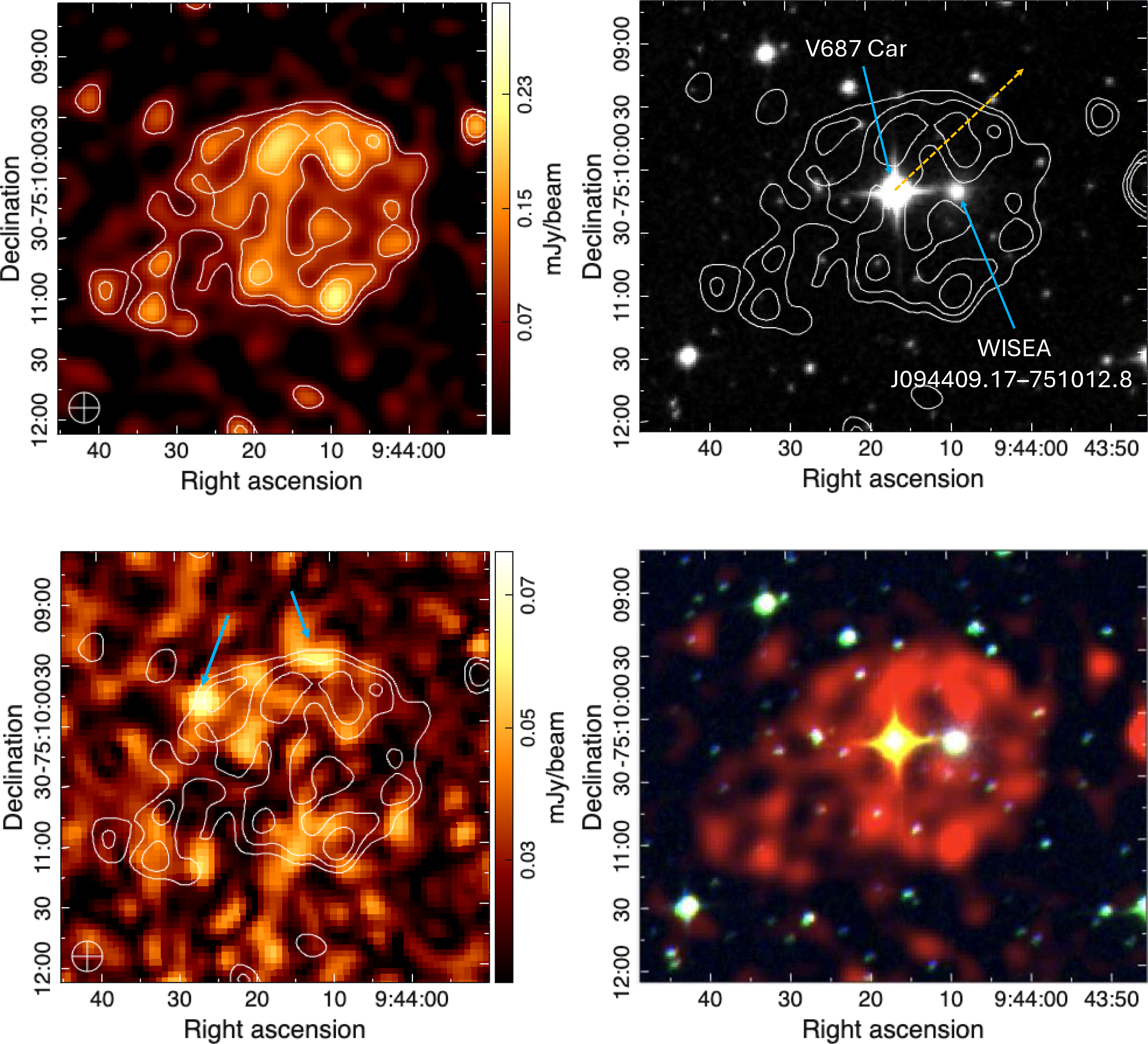


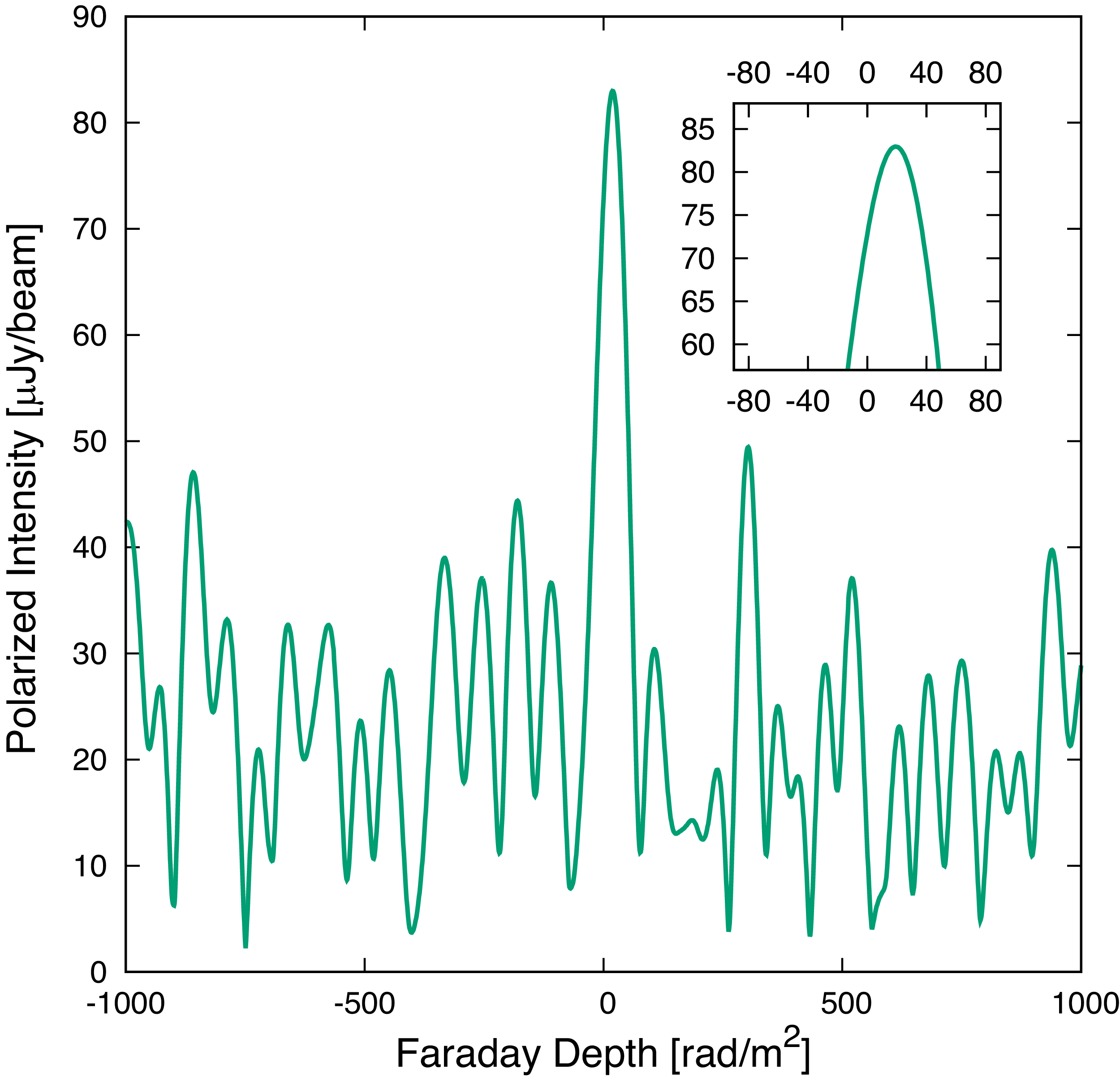
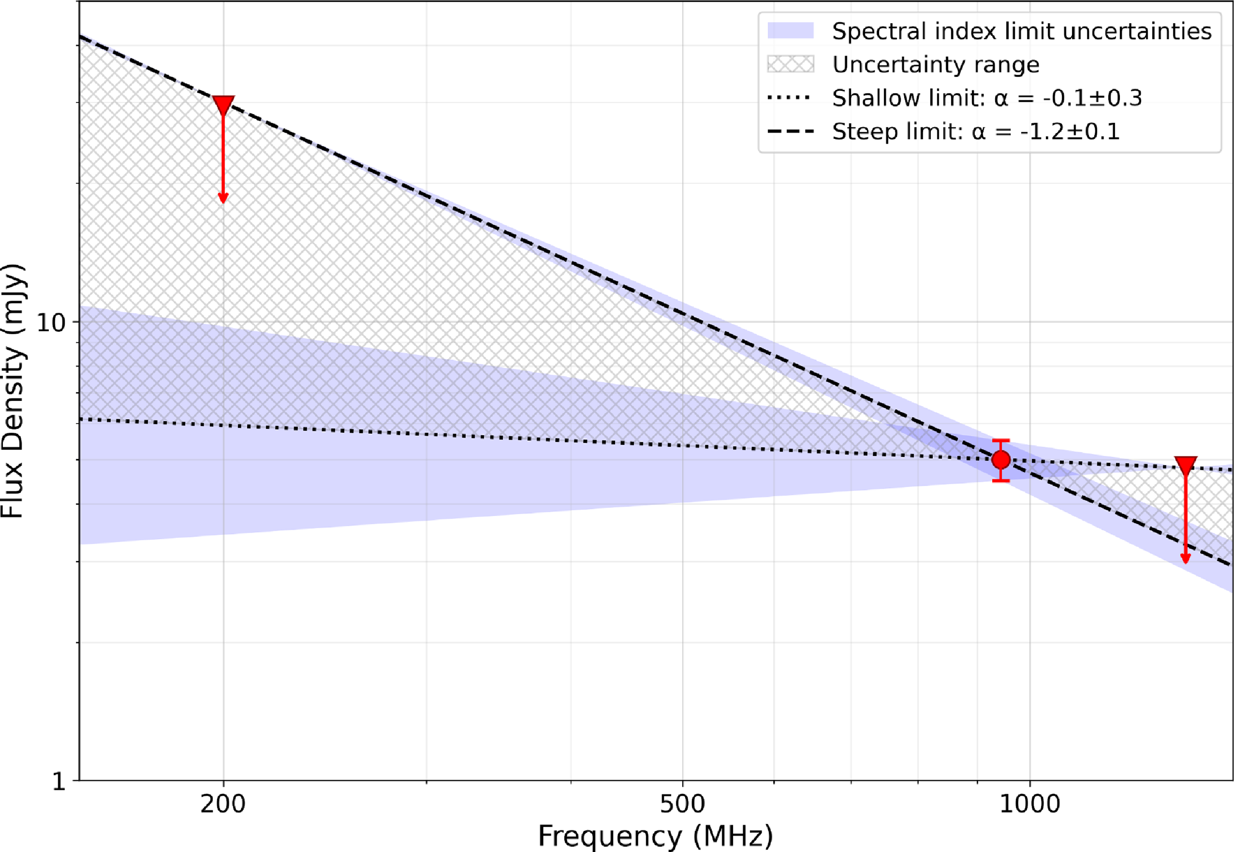
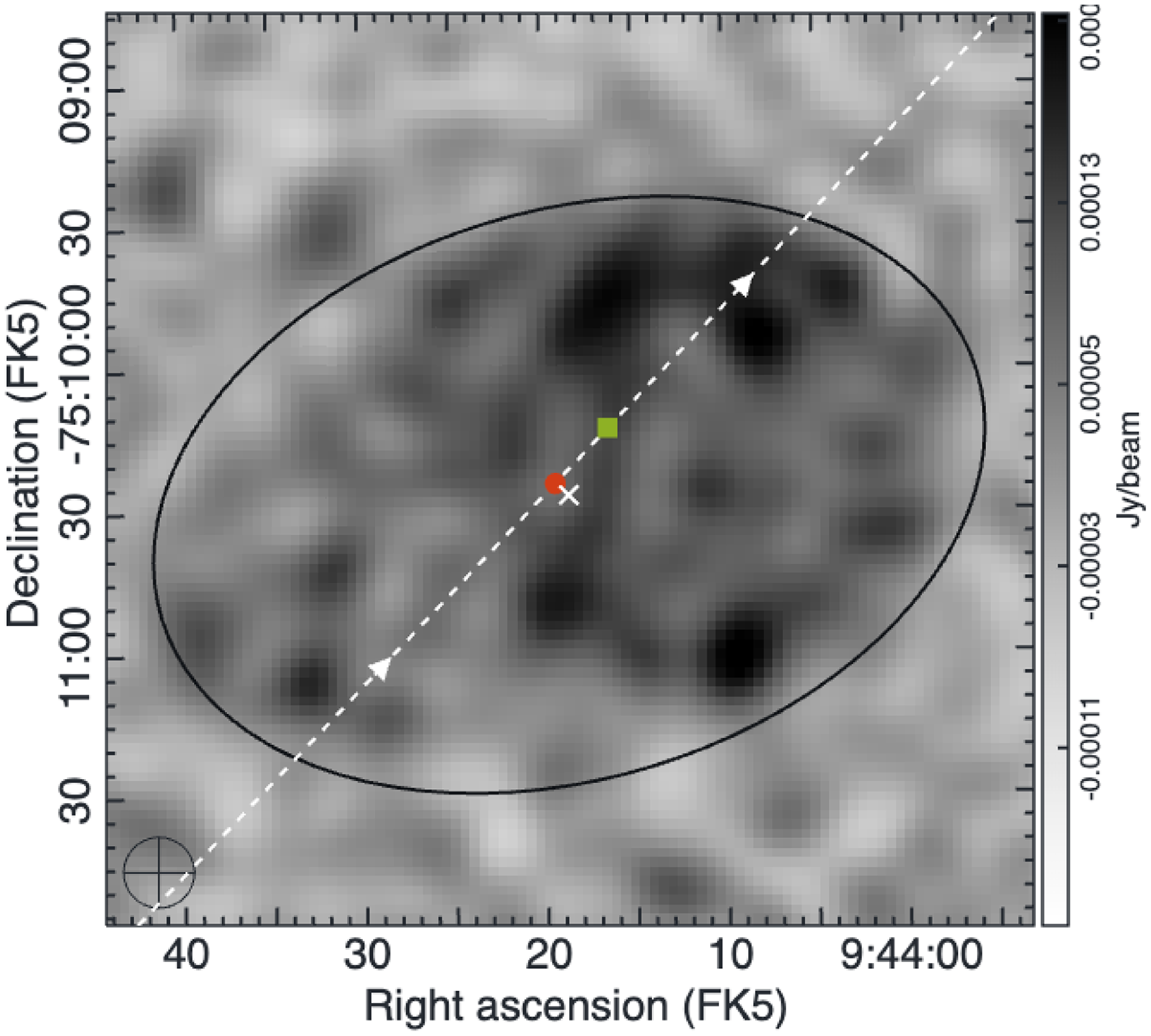
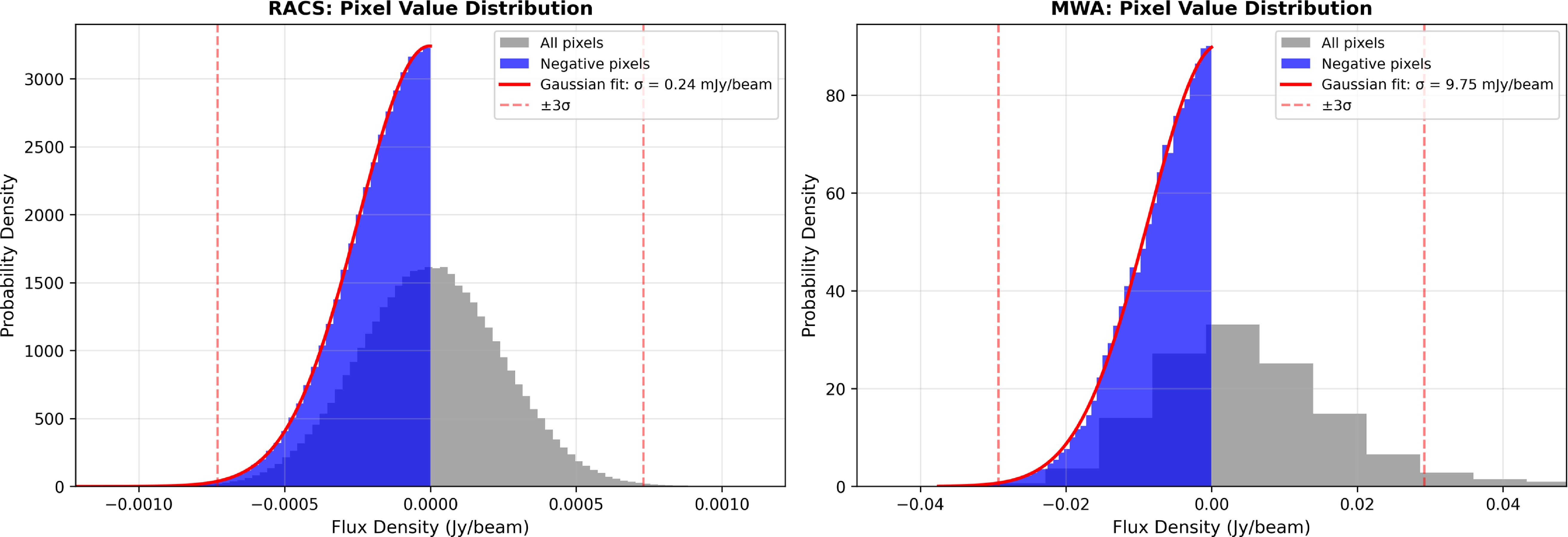


 Open access