


1. Introduction
Subjective probability estimates provided by human experts are important in many different domains, among them business, finance, marketing, politics, engineering, meteorology, environmental science, and public health (McAndrew et al., Reference McAndrew, Wattanachit, Gibson and Reich2021). In contrast to machine learning algorithms, they provide knowledge based on human intuition and experience without access to large data sets (McAndrew et al., Reference McAndrew, Wattanachit, Gibson and Reich2021). In this way, they can steer decisions and facilitate planning and dealing with risks. The subjective probability estimates can be either predictions for future events (Graefe, Reference Graefe2018; Turner et al., Reference Turner, Steyvers, Merkle, Budescu and Wallsten2014), for example, election outcomes or weather phenomena, a quantification of an expert’s belief in the truth of a statement (Karvetski et al., Reference Karvetski, Olson, Mandel and Twardy2013; Prelec et al., Reference Prelec, Seung and McCoy2017), or any other binary classifications. In the following, we will refer to these probability estimates as forecasts. Accordingly, the human subjects providing them will be termed forecasters. The subject of the forecast, for example, an event to be predicted or a statement to be judged, will be referred to as a query.
If multiple forecasts from different forecasters are available for the query at hand, combining these individual forecasts usually increases performance (Bennett et al., Reference Bennett, Benjamin, Mistry and Steyvers2018; Budescu and Chen, Reference Budescu and Chen2015; McAndrew et al., Reference McAndrew, Wattanachit, Gibson and Reich2021; Satopää, Reference Satopää2022; Satopää et al., Reference Satopää, Salikhov, Tetlock and Mellers2023; Turner et al., Reference Turner, Steyvers, Merkle, Budescu and Wallsten2014), known as the wisdom-of-the-crowds effect (Surowiecki, Reference Surowiecki2005). The combination of forecasts can be realized with behavioral or mathematical combination methods. For behavioral forecast aggregation, the forecasters negotiate a consensus in a social process (Minson et al., Reference Minson, Mueller and Larrick2018; Silver et al., Reference Silver, Mellers and Tetlock2021). In contrast, mathematical aggregation methods use mathematical fusion rules or models to combine the provided individual forecasts to an aggregated forecast (Clemen and Winkler, Reference Clemen and Winkler1999; Hanea et al., Reference Hanea, Wilkinson, McBride, Lyon, van Ravenzwaaij, Singleton Thorn, Gray, Mandel, Willcox and Gould2021; Wilson, Reference Wilson2017).
There is a wide range of different possible mathematical fusion rules for combining forecasts, which can result in different performances of the fused forecast (Satopää et al., Reference Satopää, Pemantle and Ungar2016). Many of them assume the individual forecasters to be independent (Wilson, Reference Wilson2017) or at least do not explicitly consider a possible correlation between the provided probability estimates. Popular examples of such methods are linear opinion pools, i.e., unweighted or weighted averages. While unweighted linear opinion pools, i.e., standard averages, can already achieve solid performance (Clemen, Reference Clemen1989; Turner et al., Reference Turner, Steyvers, Merkle, Budescu and Wallsten2014), weighted linear opinion pools try to increase fusion performance by giving each forecaster a different weight. The weights can be determined by the forecasters’ individual performance (Cooke, Reference Cooke1991; Hanea et al., Reference Hanea, Wilkinson, McBride, Lyon, van Ravenzwaaij, Singleton Thorn, Gray, Mandel, Willcox and Gould2021), their forecasts’ coherence (Karvetski et al., Reference Karvetski, Olson, Mandel and Twardy2013), or the number of cues available to them (Budescu and Rantilla, Reference Budescu and Rantilla2000), or can be optimized for maximum performance (Ranjan and Gneiting, Reference Ranjan and Gneiting2010). Because linear opinion pools can be over- or underconfident, trimmed (Grushka-Cockayne et al., Reference Grushka-Cockayne, Jose and Lichtendahl2017) and extremized (Baron et al., Reference Baron, Mellers, Tetlock, Stone and Ungar2014) linear opinion pools have also been proposed. Besides linear opinion pools, there are also multiplicative opinion pools, which combine forecasts using a product instead of a sum. Examples are the Independent Opinion Pool (Berger, Reference Berger1985), which explicitly assumes independent forecasts and multiplies the individual forecasts, or geometric (logarithmic) pooling (Berger, Reference Berger1985; Dietrich and List, Reference Dietrich, List, Hájek and Hitchcock2016), which is a weighted product of the forecasts. Linear as well as multiplicative opinion pools can also be used with transformations of the probability forecasts. Examples are the probit average (Satopää et al., Reference Satopää, Salikhov, Tetlock and Mellers2023), which avoids a bias of the simple average toward 0.5, or a geometric mean of odds (Satopää et al., Reference Satopää, Baron, Foster, Mellers, Tetlock and Ungar2014). In addition to the linear and multiplicative pooling methods listed above, Bayesian models for forecast aggregation have been proposed that do not consider correlations between forecasters or explicitly assume independent forecasters (Hanea et al., Reference Hanea, Wilkinson, McBride, Lyon, van Ravenzwaaij, Singleton Thorn, Gray, Mandel, Willcox and Gould2021; Trick et al., Reference Trick, Rothkopf and Jäkel2023; Turner et al., Reference Turner, Steyvers, Merkle, Budescu and Wallsten2014). Hanea et al. (Reference Hanea, Wilkinson, McBride, Lyon, van Ravenzwaaij, Singleton Thorn, Gray, Mandel, Willcox and Gould2021) propose an unsupervised Bayesian model that does not rely on historical seed queries to learn the forecasters’ behavior. In contrast, Turner et al. (Reference Turner, Steyvers, Merkle, Budescu and Wallsten2014) introduce a family of different supervised Bayesian models, which either first calibrate the forecasts and then fuse them using an unweighted linear opinion pool or vice versa. Finally, Trick et al. (Reference Trick, Rothkopf and Jäkel2023) explicitly assume independent forecasts and model them with beta distributions conditioned on the truth value.
However, human forecasters are usually correlated (Berger, Reference Berger1985; Hogarth, Reference Hogarth1978; Lichtendahl et al., Reference Lichtendahl, Grushka-Cockayne, Jose and Winkler2022; Wilson and Farrow, Reference Wilson, Farrow, Dias, Morton and Quigley2018; Winkler et al., Reference Winkler, Grushka-Cockayne, Lichtendahl and Jose2019; Wiper and French, Reference Wiper and French1995). The correlation between forecasters can be attributed to similar data seen (Morris, Reference Morris1986; Winkler, Reference Winkler1981; Winkler et al., Reference Winkler, Grushka-Cockayne, Lichtendahl and Jose2019), similar training (Lichtendahl et al., Reference Lichtendahl, Grushka-Cockayne, Jose and Winkler2022; Winkler, Reference Winkler1981; Winkler et al., Reference Winkler, Grushka-Cockayne, Lichtendahl and Jose2019), and/or similar methodology, such as statistical procedures as an aid for forecasting (Lichtendahl et al., Reference Lichtendahl, Grushka-Cockayne, Jose and Winkler2022; Morris, Reference Morris1986; Winkler, Reference Winkler1981; Winkler et al., Reference Winkler, Grushka-Cockayne, Lichtendahl and Jose2019).
If the provided forecasts are correlated but the used fusion method assumes independence, the fused forecast might be overconfident, because the amount of unique information is overestimated and thus uncertainty is reduced too much (Trick et al., Reference Trick, Rothkopf and Jäkel2023; Trick and Rothkopf, Reference Trick, Rothkopf, Camps-Valls, Ruiz and Valera2022; Wilson, Reference Wilson2017). Therefore, forecast aggregation methods should explicitly consider the forecasters’ correlation to avoid overconfidence and improve the fused forecast’s performance (Wilson, Reference Wilson2017). In fact, considering the correlation of forecasters has been declared as one of the major challenges in forecast aggregation according to the review by McAndrew et al. (Reference McAndrew, Wattanachit, Gibson and Reich2021).
There are already several approaches that explicitly propose fusion methods for correlated forecasts. Budescu and Chen (Reference Budescu and Chen2015) introduced a weighted linear opinion pool with higher weights for forecasters that are less correlated to the other forecasters. Other approaches explicitly infer the amount of shared information underlying correlated forecasts by asking the forecasters not only for their own forecast but also for an additional prediction of the other forecasters’ average forecast (Palley and Satopää, Reference Palley and Satopää2023; Palley and Soll, Reference Palley and Soll2019; Peker, Reference Peker2023; Rilling, Reference Rilling2025). Satopää (Reference Satopää2022) proposes a Bayesian model for combining correlated forecasts without additional predictions of other forecasters’ forecasts. However, their model is unsupervised, so they cannot learn the individual behavior of the forecasters, including their correlation, from historical seed queries. In contrast, the model by Babic et al. (Reference Babic, Gaba, Tsetlin and Winkler2022) relies on historical data but assumes the complete evidence that caused the forecasts to be known, which includes the amount of shared information that caused the correlation between the forecasters.
Since the concrete evidence underlying the provided forecasts is difficult to come by in practice, some Bayesian approaches model the unknown information that caused the forecasts as latent variables (Di Bacco et al., Reference Di Bacco, Frederic and Lad2003; Lichtendahl et al., Reference Lichtendahl, Grushka-Cockayne, Jose and Winkler2022; Satopää et al., Reference Satopää, Pemantle and Ungar2016). Di Bacco et al. (Reference Di Bacco, Frederic and Lad2003) consider two forecasters that provide their probabilistic forecasts for an event H. Their model assumes some knowledge that both forecasters share and some knowledge that only specific forecasters have, represented as events F,
 $G_1$
, and
$G_1$
, and
 $G_2$
. The provided forecasts are transformed to odds and modeled with a log-normal distribution, jointly with the ratios of the posterior distributions of H given F, H given
$G_2$
. The provided forecasts are transformed to odds and modeled with a log-normal distribution, jointly with the ratios of the posterior distributions of H given F, H given
 $G_1$
, and H given
$G_1$
, and H given
 $G_2$
. However, their approach is rather theoretical. It remains unclear how to get the model parameters from prior experience. Satopää et al. (Reference Satopää, Pemantle and Ungar2016) propose a partial information framework for the aggregation of K forecasters. They model the information underlying the forecasts as particles of information, either positive or negative. If the sum of all particles
$G_2$
. However, their approach is rather theoretical. It remains unclear how to get the model parameters from prior experience. Satopää et al. (Reference Satopää, Pemantle and Ungar2016) propose a partial information framework for the aggregation of K forecasters. They model the information underlying the forecasts as particles of information, either positive or negative. If the sum of all particles
 $X_S$
is positive, the event happens. Each forecaster observes some particle subset
$X_S$
is positive, the event happens. Each forecaster observes some particle subset
 $B_i$
, and the subsets of different forecasters can overlap, which generates a correlation between their forecasts. The sums of particles
$B_i$
, and the subsets of different forecasters can overlap, which generates a correlation between their forecasts. The sums of particles
 $X_S, X_{B_1}, \dots , X_{B_K}$
are modeled with a multivariate normal distribution with mean 0 and covariances equal to the number of shared particles in different subsets. The sum of particles
$X_S, X_{B_1}, \dots , X_{B_K}$
are modeled with a multivariate normal distribution with mean 0 and covariances equal to the number of shared particles in different subsets. The sum of particles
 $X_{B_i}$
is transformed to a probability forecast with probit transformation. With their model, Satopää et al. (Reference Satopää, Pemantle and Ungar2016) show when averages of forecasts should be extremized, i.e., shifted toward 0 or 1, and how this is dependent on how much information the forecasters share. With a similar goal, Lichtendahl et al. (Reference Lichtendahl, Grushka-Cockayne, Jose and Winkler2022) also model the information causing the forecasts as information particles
$X_{B_i}$
is transformed to a probability forecast with probit transformation. With their model, Satopää et al. (Reference Satopää, Pemantle and Ungar2016) show when averages of forecasts should be extremized, i.e., shifted toward 0 or 1, and how this is dependent on how much information the forecasters share. With a similar goal, Lichtendahl et al. (Reference Lichtendahl, Grushka-Cockayne, Jose and Winkler2022) also model the information causing the forecasts as information particles
 $x_i$
. Some information particles are private for individual forecasters, some are shared between all forecasters. All information particles
$x_i$
. Some information particles are private for individual forecasters, some are shared between all forecasters. All information particles
 $x_i$
as well as the target variable
$x_i$
as well as the target variable
 $x_t$
, whose value determines the truth value t, are distributed under the same distribution with a conjugate prior on its parameters. By applying Bayes’ rule, the posterior probability of the target variable
$x_t$
, whose value determines the truth value t, are distributed under the same distribution with a conjugate prior on its parameters. By applying Bayes’ rule, the posterior probability of the target variable
 $x_t$
is computed as the fusion result given some sufficient statistics of observed information particles
$x_t$
is computed as the fusion result given some sufficient statistics of observed information particles
 $x_i$
, which are in turn computed from the observed probabilistic forecasts provided by the forecasters. The unknown sufficient statistics from the shared information particles are integrated out. Two specific conjugate models are discussed, Beta-Bernoulli and Normal-Normal. However, to be applicable to real data, the model is simplified: It is assumed that the probability of the truth value t given all provided forecasts is a generalized linear model.
$x_i$
, which are in turn computed from the observed probabilistic forecasts provided by the forecasters. The unknown sufficient statistics from the shared information particles are integrated out. Two specific conjugate models are discussed, Beta-Bernoulli and Normal-Normal. However, to be applicable to real data, the model is simplified: It is assumed that the probability of the truth value t given all provided forecasts is a generalized linear model.
In contrast to the models presented above, which explicitly model the latent information causing the provided forecasts, other Bayesian models only model the provided probability forecasts as data (Bordley, Reference Bordley1982; Clemen and Winkler, Reference Clemen, Winkler and Viertl1987; French, Reference French1980). French (Reference French1980) as well as Clemen and Winkler (Reference Clemen, Winkler and Viertl1987) transfer the probability estimates to log-odds and model them with a multivariate Gaussian distribution conditioned on the truth value t. With their model and some historical training data, they can learn how individual forecasters behave for true and false queries, i.e., their bias, variance, and uncertainty. Also, using the Gaussian distribution, they can model pairwise correlation between individual forecasters. Bordley (Reference Bordley1982) uses the same multivariate Gaussian model approach in order to derive the weights for a multiplicative fusion rule considering the correlation of forecasters.
While transforming the probability forecasts to log-odds and modeling them with a multivariate Gaussian distribution is mathematically convenient and enables straightforward representation of correlations between forecasts, another possibility is to model them directly with a beta distribution without any transformation. The beta distribution is commonly used to model probabilities since it is the standard distribution over probabilities in Bayesian statistics and the conjugate prior of the Bernoulli distribution. Accordingly, in prior work, we modeled probabilistic forecasts with a beta distribution conditioned on the truth value t (Trick et al., Reference Trick, Rothkopf and Jäkel2023) and used this model for normative aggregation of probability forecasts. However, in that model, we assumed the forecasts provided by different forecasters to be conditionally independent given the truth value t. This assumption, which usually does not hold in reality, caused our beta fusion model to be overconfident on two real-world data sets. Thus, for correlated forecasts, this model is not normative. It does not formalize how to obtain the correct fused uncertainty.
Therefore, in the present work, we introduce a Bayesian model for combining probabilistic forecasts that considers the correlation between forecasts. The new model also represents the forecasts with a beta distribution conditioned on the truth value t. However, in our model, we additionally assume that the forecast provided by a forecaster for a query depends on an interplay of the forecaster’s skill and the query’s difficulty. Moreover, we assume that the correlation between forecasts provided by different forecasters can be attributed to the fact that they answer to the same queries since for all forecasters some queries are easy and others are hard. The resulting Skill–Difficulty Correlated Fusion Model explicitly models the forecasters’ skills and the queries’ difficulties and thereby implicitly models the correlation between forecasts, which can then be considered for fusion. Fusing forecasts according to the Skill–Difficulty Correlated Fusion Model is normative, given that the model assumptions are correct. In particular, correlated forecasts can be fused normatively.
The remainder of the article is structured as follows. Section 2 introduces our new Skill–Difficulty Correlated Fusion Model, including its generative model and a discussion of its parameters, a reparameterization in favor of interpretability and inference, the correlations that can be represented, as well as parameter inference and fusion. In Section 3, we present our evaluations of the model, including a detailed description of the used data set and cross-validation, an evaluation of how the estimated model parameters can be interpreted and how our model fits the data, and a comparison of the Skill–Difficulty Correlated Fusion Model’s fusion performance to related Bayesian models. Finally, we discuss our results and outline conclusions, limitations, and ideas for future work in Section 4.
2. The Skill–Difficulty Correlated Fusion Model
We propose the Skill–Difficulty Correlated Fusion Model, a Bayesian generative model for combining probabilistic forecasts provided by human forecasters, which explicitly models the forecasters’ skills and the queries’ difficulties in order to implicitly model the correlation between forecasts. After introducing the generative model in Section 2.1, we discuss the model parameters’ interpretation in Section 2.2. In Section 2.3, we introduce a reparameterization of the model in favor of parameter interpretability and robustness of inference and discuss the correlations that can be represented using the model in Section 2.4. In Section 2.5, we outline parameter inference and fusion with the model.
2.1. Generative model
We assume K human forecasters to provide subjective probability estimates, i.e., forecasts, on N binary queries. The queries can be factual statements that are either true or false, questions that can be answered with yes or no, or any other binary classification task with a truth value of either 1 or 0. For each query, the probability estimates provided by the forecasters quantify their belief in their answer’s correctness. A probability of 0 indicates that the forecaster is completely certain that the query’s truth value is 0 (e.g., false/no), whereas a probability of 1 means that the forecaster assumes a truth value of 1 (e.g., true/yes) with full certainty.
We formalize the forecast provided by forecaster k for query n as
 $x_n^k \in [0,1]$
with
$x_n^k \in [0,1]$
with
 $n = 1, \dots , N$
,
$n = 1, \dots , N$
,
 $k = 1, \dots , K$
. The truth value of query n is formalized as
$k = 1, \dots , K$
. The truth value of query n is formalized as
 $t_n \in \{0,1\}$
for
$t_n \in \{0,1\}$
for
 $n = 1, \dots , N$
. Since the beta distribution is the natural choice for modeling probabilities, a previous model (Trick et al., Reference Trick, Rothkopf and Jäkel2023) assumes the forecasts
$n = 1, \dots , N$
. Since the beta distribution is the natural choice for modeling probabilities, a previous model (Trick et al., Reference Trick, Rothkopf and Jäkel2023) assumes the forecasts
 $x_n^k$
to be beta-distributed conditioned on the truth value
$x_n^k$
to be beta-distributed conditioned on the truth value
 $t_n \in \{0,1\}$
, as
$t_n \in \{0,1\}$
, as
 $$ \begin{align} x_n^k | t_n = j &\sim \text{Beta}(\alpha_j^k, \beta_j^k), \quad j=0,1. \end{align} $$
After learning the parameters
 $\alpha _j^k$
and
$\alpha _j^k$
and
 $\beta _j^k$
from labeled training data, this model represents the forecasting behavior of each forecaster conditioned on the truth value
$\beta _j^k$
from labeled training data, this model represents the forecasting behavior of each forecaster conditioned on the truth value
 $t_n$
, including their bias, uncertainty, and variance. In particular, forecaster k’s bias can be expressed with the beta distribution’s mean
$t_n$
, including their bias, uncertainty, and variance. In particular, forecaster k’s bias can be expressed with the beta distribution’s mean
 $\mu _j^k=\alpha _j^k/(\alpha _j^k+\beta _j^k)$
. If
$\mu _j^k=\alpha _j^k/(\alpha _j^k+\beta _j^k)$
. If
 $\mu _0^k<0.5$
and
$\mu _0^k<0.5$
and
 $\mu _1^k>0.5$
, we define forecaster k to be unbiased since they on average provide correct forecasts. The mean forecast
$\mu _1^k>0.5$
, we define forecaster k to be unbiased since they on average provide correct forecasts. The mean forecast
 $\mu _j^k$
can also quantify the uncertainty of forecaster k: The closer it is to 0 or 1, the less uncertain the forecaster is on average. However, the uncertainty of the actual forecasts provided by forecaster k is also dependent on their variance, which determines their forecasts’ concentration around the mean
$\mu _j^k$
can also quantify the uncertainty of forecaster k: The closer it is to 0 or 1, the less uncertain the forecaster is on average. However, the uncertainty of the actual forecasts provided by forecaster k is also dependent on their variance, which determines their forecasts’ concentration around the mean
 $\mu _j^k$
. This variance can be expressed with the modeling beta distribution’s precision
$\mu _j^k$
. This variance can be expressed with the modeling beta distribution’s precision
 $p_j^k=\alpha _j^k + \beta _j^k$
, also known as its concentration parameter (Huang, Reference Huang2005). The higher this precision is, the lower is the beta distribution’s variance. Still, note that it is not the inverse of the distribution’s variance. While explicitly considering the learned behavior of the forecasts, i.e., their bias, uncertainty, and variance, new forecasts
$p_j^k=\alpha _j^k + \beta _j^k$
, also known as its concentration parameter (Huang, Reference Huang2005). The higher this precision is, the lower is the beta distribution’s variance. Still, note that it is not the inverse of the distribution’s variance. While explicitly considering the learned behavior of the forecasts, i.e., their bias, uncertainty, and variance, new forecasts
 $x_u^k$
for a previously unseen query u can be fused by inferring the truth value
$x_u^k$
for a previously unseen query u can be fused by inferring the truth value
 $t_u$
given the forecasts
$t_u$
given the forecasts
 $x_u^k$
and the learned parameters
$x_u^k$
and the learned parameters
 $\alpha _j^k$
and
$\alpha _j^k$
and
 $\beta _j^k$
using Bayes’ rule. Note that by modeling bias, variance, and uncertainty with a beta distribution conditioned on the truth value
$\beta _j^k$
using Bayes’ rule. Note that by modeling bias, variance, and uncertainty with a beta distribution conditioned on the truth value
 $t_n$
, the forecasters are also implicitly calibrated when they are fused. This means that they are corrected for over- or underconfident forecasts, which do not match the relative frequency of occurrence, for example, of a predicted event or a judged true statement (Trick et al., Reference Trick, Rothkopf and Jäkel2023).
$t_n$
, the forecasters are also implicitly calibrated when they are fused. This means that they are corrected for over- or underconfident forecasts, which do not match the relative frequency of occurrence, for example, of a predicted event or a judged true statement (Trick et al., Reference Trick, Rothkopf and Jäkel2023).
In previous work, four variants of this beta fusion model were compared (Trick et al., Reference Trick, Rothkopf and Jäkel2023). While in (2.1), the forecasts are modeled with two completely different beta distributions for
 $t_n=0$
and
$t_n=0$
and
 $t_n=1$
, the symmetric variant of the model represents the forecasts with symmetric beta distributions for
$t_n=1$
, the symmetric variant of the model represents the forecasts with symmetric beta distributions for
 $t_n=0$
and
$t_n=0$
and
 $t_n=1$
, i.e., as
$t_n=1$
, i.e., as
 $$ \begin{align} \begin{aligned} x_n^k | t_n = 0 &\sim \text{Beta}(\alpha^k, \beta^k)\\ x_n^k | t_n = 1 &\sim \text{Beta}(\beta^k, \alpha^k). \end{aligned} \end{align} $$
Thus, it assumes the forecasts provided for queries with truth values
 $t_n=0$
and the ones for queries with truth values
$t_n=0$
and the ones for queries with truth values
 $t_n=1$
to be symmetric around 0.5. This symmetric beta fusion model is of special interest because it implicitly calibrates the forecasts according to a well-known calibration function, the Linear-in-Log-Odds calibration function (Trick et al., Reference Trick, Rothkopf and Jäkel2023). For both the asymmetric (2.1) and the symmetric (2.2) variant of the model, which model each forecaster k separately with hierarchical models, we also investigated non-hierarchical model variants, which consider the forecasters as exchangeable and only learn one parameter set for all of them.
$t_n=1$
to be symmetric around 0.5. This symmetric beta fusion model is of special interest because it implicitly calibrates the forecasts according to a well-known calibration function, the Linear-in-Log-Odds calibration function (Trick et al., Reference Trick, Rothkopf and Jäkel2023). For both the asymmetric (2.1) and the symmetric (2.2) variant of the model, which model each forecaster k separately with hierarchical models, we also investigated non-hierarchical model variants, which consider the forecasters as exchangeable and only learn one parameter set for all of them.
All variants of the beta fusion model shown above assume the forecasts
 $x_n^k$
provided by different forecasters k to be conditionally independent given the truth value
$x_n^k$
provided by different forecasters k to be conditionally independent given the truth value
 $t_n$
. However, for real-world forecasting data, this assumption is usually not met (Berger, Reference Berger1985; Hogarth, Reference Hogarth1978; Lichtendahl et al., Reference Lichtendahl, Grushka-Cockayne, Jose and Winkler2022; Wilson and Farrow, Reference Wilson, Farrow, Dias, Morton and Quigley2018; Winkler et al., Reference Winkler, Grushka-Cockayne, Lichtendahl and Jose2019; Wiper and French, Reference Wiper and French1995). Accordingly, our evaluations on two data sets also showed that the beta fusion models are overconfident, which deteriorates their performance. Therefore, in this work, we extend the beta fusion model to consider correlations between forecasters.
$t_n$
. However, for real-world forecasting data, this assumption is usually not met (Berger, Reference Berger1985; Hogarth, Reference Hogarth1978; Lichtendahl et al., Reference Lichtendahl, Grushka-Cockayne, Jose and Winkler2022; Wilson and Farrow, Reference Wilson, Farrow, Dias, Morton and Quigley2018; Winkler et al., Reference Winkler, Grushka-Cockayne, Lichtendahl and Jose2019; Wiper and French, Reference Wiper and French1995). Accordingly, our evaluations on two data sets also showed that the beta fusion models are overconfident, which deteriorates their performance. Therefore, in this work, we extend the beta fusion model to consider correlations between forecasters.
In line with the previous beta fusion models, in our new Skill–Difficulty Correlated Fusion Model, we also model the forecasts
 $x_n^k$
with a beta distribution conditioned on the truth value
$x_n^k$
with a beta distribution conditioned on the truth value
 $t_n$
. Likewise, we also assume symmetric beta distributions for modeling forecasts with truth value
$t_n$
. Likewise, we also assume symmetric beta distributions for modeling forecasts with truth value
 $t_n=0$
and
$t_n=0$
and
 $t_n=1$
as in (2.2), because previous evaluations showed that symmetric beta modeling leads to more robust calibration and higher fusion performance (Trick et al., Reference Trick, Rothkopf and Jäkel2023). However, we do not assume that forecast
$t_n=1$
as in (2.2), because previous evaluations showed that symmetric beta modeling leads to more robust calibration and higher fusion performance (Trick et al., Reference Trick, Rothkopf and Jäkel2023). However, we do not assume that forecast
 $x_n^k$
by forecaster k for query n is generated merely by the forecaster’s behavior and can thus be modeled with a beta distribution with parameters
$x_n^k$
by forecaster k for query n is generated merely by the forecaster’s behavior and can thus be modeled with a beta distribution with parameters
 $\alpha ^k,\beta ^k$
specific for this forecaster k. Instead, here, we assume that forecast
$\alpha ^k,\beta ^k$
specific for this forecaster k. Instead, here, we assume that forecast
 $x_n^k$
by forecaster k for query n is generated by both forecaster k’s properties, which we call their skill, and query n’s properties, which we call its difficulty. Accordingly, we model
$x_n^k$
by forecaster k for query n is generated by both forecaster k’s properties, which we call their skill, and query n’s properties, which we call its difficulty. Accordingly, we model
 $x_n^k$
with a beta distribution with parameters
$x_n^k$
with a beta distribution with parameters
 $\alpha _k$
and
$\alpha _k$
and
 $\beta _k$
, specific for forecaster k, and parameters
$\beta _k$
, specific for forecaster k, and parameters
 $\gamma _n$
and
$\gamma _n$
and
 $\delta _n$
, specific for query n. In particular, if
$\delta _n$
, specific for query n. In particular, if
 $t_n=0$
,
$t_n=0$
,
 $x_n^k$
is modeled with a beta distribution with parameters
$x_n^k$
is modeled with a beta distribution with parameters
 $\alpha _k + \gamma _n$
and
$\alpha _k + \gamma _n$
and
 $\beta _k + \delta _n$
. If
$\beta _k + \delta _n$
. If
 $t_n=1,$
the parameters are interchanged to
$t_n=1,$
the parameters are interchanged to
 $\beta _k+\delta _n$
and
$\beta _k+\delta _n$
and
 $\alpha _k+\gamma _n$
,
$\alpha _k+\gamma _n$
,
 $$ \begin{align} \begin{aligned} x_n^k | t_n=0 &\sim \text{Beta}(\alpha_k+\gamma_n, \beta_k+\delta_n)\\ x_n^k | t_n=1 &\sim \text{Beta}(\beta_k+\delta_n, \alpha_k+\gamma_n). \end{aligned} \end{align} $$
The prior distribution on the truth value
 $t_n$
is a Bernoulli distribution with parameter
$t_n$
is a Bernoulli distribution with parameter
 $\pi $
, which is the proportion of true queries with truth value 1. The graphical model of the Skill–Difficulty Correlated Fusion Model is shown in Figure 1.
$\pi $
, which is the proportion of true queries with truth value 1. The graphical model of the Skill–Difficulty Correlated Fusion Model is shown in Figure 1.
The graphical model of the Skill–Difficulty Correlated Fusion Model.

2.2. Interpretation of the model’s parameters as skill and difficulty
The parameters
 $\alpha _k$
and
$\alpha _k$
and
 $\beta _k$
represent something akin to the skill of forecaster k in the sense that they determine the bias, variance, and uncertainty of forecasts provided by forecaster k independently of the query at hand n. Therefore, in the following,
$\beta _k$
represent something akin to the skill of forecaster k in the sense that they determine the bias, variance, and uncertainty of forecasts provided by forecaster k independently of the query at hand n. Therefore, in the following,
 $\alpha _k$
and
$\alpha _k$
and
 $\beta _k$
will be termed skill parameters. Equivalently, the parameters
$\beta _k$
will be termed skill parameters. Equivalently, the parameters
 $\gamma _n$
and
$\gamma _n$
and
 $\delta _n$
represent the difficulty of query n since they determine the bias, variance, and uncertainty of forecasts provided for query n independently of the specific forecasters providing them. Accordingly, we call
$\delta _n$
represent the difficulty of query n since they determine the bias, variance, and uncertainty of forecasts provided for query n independently of the specific forecasters providing them. Accordingly, we call
 $\gamma _n$
and
$\gamma _n$
and
 $\delta _n$
difficulty parameters.
$\delta _n$
difficulty parameters.
For interpreting the skill parameters
 $\alpha _k$
and
$\alpha _k$
and
 $\beta _k$
isolated from the difficulty parameters
$\beta _k$
isolated from the difficulty parameters
 $\gamma _n$
and
$\gamma _n$
and
 $\delta _n$
, we can set the difficulty parameters
$\delta _n$
, we can set the difficulty parameters
 $\gamma _n$
and
$\gamma _n$
and
 $\delta _n$
close to 0, meaning that only the forecasters’ properties are determining the forecasts. In this case, forecasts
$\delta _n$
close to 0, meaning that only the forecasters’ properties are determining the forecasts. In this case, forecasts
 $x_n^k$
are distributed according to Beta(
$x_n^k$
are distributed according to Beta(
 $\alpha _k, \beta _k$
) for
$\alpha _k, \beta _k$
) for
 $t_n=0$
and Beta(
$t_n=0$
and Beta(
 $\beta _k, \alpha _k$
) for
$\beta _k, \alpha _k$
) for
 $t_n=1$
. Note that with this parametrization, our Skill–Difficulty Correlated Fusion Model equals the symmetric variant of the previously proposed independent beta fusion model in (2.2). If for real data the difficulty parameters
$t_n=1$
. Note that with this parametrization, our Skill–Difficulty Correlated Fusion Model equals the symmetric variant of the previously proposed independent beta fusion model in (2.2). If for real data the difficulty parameters
 $\gamma _n$
and
$\gamma _n$
and
 $\delta _n$
are not equal to 0, the distributions Beta(
$\delta _n$
are not equal to 0, the distributions Beta(
 $\alpha _k, \beta _k$
) for
$\alpha _k, \beta _k$
) for
 $t_n=0$
and Beta(
$t_n=0$
and Beta(
 $\beta _k, \alpha _k$
) for
$\beta _k, \alpha _k$
) for
 $t_n=1$
do not describe the forecasts
$t_n=1$
do not describe the forecasts
 $x_n^k$
. However, they describe the forecasts we would assume if the queries’ difficulties had no influence on forecaster k’s forecasts. Forecaster k’s bias, which in part defines their skill, is determined by the mean of this beta distribution for
$x_n^k$
. However, they describe the forecasts we would assume if the queries’ difficulties had no influence on forecaster k’s forecasts. Forecaster k’s bias, which in part defines their skill, is determined by the mean of this beta distribution for
 $t_n=0$
, which is
$t_n=0$
, which is
 $\mu _k=\alpha _k/(\alpha _k+\beta _k)$
. This skill mean describes the average forecast we would expect if the queries’ difficulties had no influence on forecaster k’s forecasts. If
$\mu _k=\alpha _k/(\alpha _k+\beta _k)$
. This skill mean describes the average forecast we would expect if the queries’ difficulties had no influence on forecaster k’s forecasts. If
 $\mu _k<0.5$
, we define forecaster k to be unbiased because their mean forecast is closer to the truth value
$\mu _k<0.5$
, we define forecaster k to be unbiased because their mean forecast is closer to the truth value
 $t_n$
, so a forced binary decision for the discrete truth value (i.e., 0 or 1) would correctly correspond to the truth value. Thus, if
$t_n$
, so a forced binary decision for the discrete truth value (i.e., 0 or 1) would correctly correspond to the truth value. Thus, if
 $\beta _k>\alpha _k$
, forecaster k is unbiased. Forecaster k’s skill is also determined by their uncertainty, which is also quantified by the skill mean
$\beta _k>\alpha _k$
, forecaster k is unbiased. Forecaster k’s skill is also determined by their uncertainty, which is also quantified by the skill mean
 $\mu _k$
. The more uncertain, i.e., the closer to 0.5 it is, the more uncertain is forecaster k on average. However, the skill mean
$\mu _k$
. The more uncertain, i.e., the closer to 0.5 it is, the more uncertain is forecaster k on average. However, the skill mean
 $\mu _k$
can only provide information on the average uncertainty, not on the actual uncertainties of different forecasts provided, since there might be variance in the provided forecasts. The variance or variability of forecaster k around their skill mean, which is also part of their skill, can be straightforwardly quantified with the beta distribution’s skill precision
$\mu _k$
can only provide information on the average uncertainty, not on the actual uncertainties of different forecasts provided, since there might be variance in the provided forecasts. The variance or variability of forecaster k around their skill mean, which is also part of their skill, can be straightforwardly quantified with the beta distribution’s skill precision
 $\rho _k=\alpha _k+\beta _k$
. Thereby, lower precisions indicate higher variance around the mean.
$\rho _k=\alpha _k+\beta _k$
. Thereby, lower precisions indicate higher variance around the mean.
The skill parameters
 $\alpha _k$
and
$\alpha _k$
and
 $\beta _k$
and the derived skill mean
$\beta _k$
and the derived skill mean
 $\mu _k$
and skill precision
$\mu _k$
and skill precision
 $\rho _k$
can identify prototypical forecasters. Given that we assume the queries’ difficulties to have no impact on their forecasts, a highly skilled forecaster provides unbiased and certain forecasts with low variance and will thus show a skill mean
$\rho _k$
can identify prototypical forecasters. Given that we assume the queries’ difficulties to have no impact on their forecasts, a highly skilled forecaster provides unbiased and certain forecasts with low variance and will thus show a skill mean
 $\mu _k$
close to 0 with high skill precision. An uncertain forecaster provides forecasts close to 0.5 with low variance with
$\mu _k$
close to 0 with high skill precision. An uncertain forecaster provides forecasts close to 0.5 with low variance with
 $\mu _k$
close to 0.5 and a high skill precision. If
$\mu _k$
close to 0.5 and a high skill precision. If
 $\mu _k$
is close to 1 with high skill precision, forecaster k is a wrong forecaster with a strong bias and thus always provides incorrect forecasts with low uncertainty and low variance and might not have understood the task correctly or is malingering.
$\mu _k$
is close to 1 with high skill precision, forecaster k is a wrong forecaster with a strong bias and thus always provides incorrect forecasts with low uncertainty and low variance and might not have understood the task correctly or is malingering.
The difficulty parameters
 $\gamma _n$
and
$\gamma _n$
and
 $\delta _n$
can be interpreted when setting the skill parameters
$\delta _n$
can be interpreted when setting the skill parameters
 $\alpha _k$
and
$\alpha _k$
and
 $\beta _k$
close to 0. As a consequence,
$\beta _k$
close to 0. As a consequence,
 $x_n^k$
are distributed according to Beta(
$x_n^k$
are distributed according to Beta(
 $\gamma _n, \delta _n$
) for
$\gamma _n, \delta _n$
) for
 $t_n=0$
and Beta(
$t_n=0$
and Beta(
 $\delta _n, \gamma _n$
) for
$\delta _n, \gamma _n$
) for
 $t_n=1$
. Although these distributions might not model real forecasts, which are also determined by the skills of the forecasters providing them, they describe the forecasts we would assume to be provided for query n if the forecasters’ skills had no impact on the forecasts. The mean of this distribution for
$t_n=1$
. Although these distributions might not model real forecasts, which are also determined by the skills of the forecasters providing them, they describe the forecasts we would assume to be provided for query n if the forecasters’ skills had no impact on the forecasts. The mean of this distribution for
 $t_n=0$
, the difficulty mean
$t_n=0$
, the difficulty mean
 $\eta _n = \gamma _n/(\gamma _n+\delta _n)$
, quantifies the average forecast for query n if the forecasters’ skills had no impact on the forecasts provided for query n. It determines the bias of the forecasts provided for query n, which partly defines its difficulty. If the difficulty mean
$\eta _n = \gamma _n/(\gamma _n+\delta _n)$
, quantifies the average forecast for query n if the forecasters’ skills had no impact on the forecasts provided for query n. It determines the bias of the forecasts provided for query n, which partly defines its difficulty. If the difficulty mean
 $\eta _n<0.5$
, hence if
$\eta _n<0.5$
, hence if
 $\delta _n>\gamma _n$
, the forecasts for query n are unbiased. Thus, the forecasters on average provide correct answers for the query, so it is rather easy. Its difficulty is, however, also determined by the uncertainty of the forecasts provided. The average uncertainty of the forecasts provided for query n is quantified by the uncertainty of the difficulty mean
$\delta _n>\gamma _n$
, the forecasts for query n are unbiased. Thus, the forecasters on average provide correct answers for the query, so it is rather easy. Its difficulty is, however, also determined by the uncertainty of the forecasts provided. The average uncertainty of the forecasts provided for query n is quantified by the uncertainty of the difficulty mean
 $\eta _n$
. More extreme difficulty means closer to 0 or 1 show lower average uncertainty of the forecasts provided for a query. The difficulty precision
$\eta _n$
. More extreme difficulty means closer to 0 or 1 show lower average uncertainty of the forecasts provided for a query. The difficulty precision
 $\phi _n=\gamma _n+\delta _n$
quantifies how concentrated the forecasts provided for query n are around the difficulty mean
$\phi _n=\gamma _n+\delta _n$
quantifies how concentrated the forecasts provided for query n are around the difficulty mean
 $\eta _n$
, i.e., their variance.
$\eta _n$
, i.e., their variance.
Given difficulty mean
 $\eta _n$
and difficulty precision
$\eta _n$
and difficulty precision
 $\phi _n$
, we can identify special queries. If
$\phi _n$
, we can identify special queries. If
 $\eta _n$
is close to 0 with high difficulty precision, query n is a very easy query, for which forecasters provide unbiased and certain forecasts with low variance, given that we assume the forecasters’ skills to have no impact on the forecasts provided for it. For difficult queries, we distinguish between two types of queries, unknown and trick queries. For unknown queries,
$\eta _n$
is close to 0 with high difficulty precision, query n is a very easy query, for which forecasters provide unbiased and certain forecasts with low variance, given that we assume the forecasters’ skills to have no impact on the forecasts provided for it. For difficult queries, we distinguish between two types of queries, unknown and trick queries. For unknown queries,
 $\eta _n$
is close to 0.5 with high difficulty precision, so the forecasters do not know the answer to the query and therefore provide uncertain forecasts close to 0.5 with low variance. In contrast, for trick queries, they provide certain but biased forecasts with low variance because they think they know the correct answer but do not. In this case,
$\eta _n$
is close to 0.5 with high difficulty precision, so the forecasters do not know the answer to the query and therefore provide uncertain forecasts close to 0.5 with low variance. In contrast, for trick queries, they provide certain but biased forecasts with low variance because they think they know the correct answer but do not. In this case,
 $\eta _n$
is close to 1 with high difficulty precision.
$\eta _n$
is close to 1 with high difficulty precision.
Note that although we define skill as a property of the forecasters and difficulty as a property of the queries, both the skills of forecasters and the difficulties of queries can be explained by the information that the considered forecasters have. A query can only be unknown if most forecasters lack information about it. At the same time, an easy query requires a majority of forecasters to share correct information about the query, while a trick query requires most forecasters to share incorrect information about it. In contrast, the skill of a forecaster can be attributed to the private information of that individual forecaster.
2.3. Model reparameterization
Since skill and difficulty can be straightforwardly quantified with the skill mean and precision and difficulty mean and precision (Section 2.2), we reparameterized the Skill–Difficulty Correlated Fusion Model: Instead of parameterizing the beta distribution with
 $\alpha $
and
$\alpha $
and
 $\beta ,$
we now use the beta distribution’s mean
$\beta ,$
we now use the beta distribution’s mean
 $\mu = \alpha / (\alpha + \beta )$
and precision
$\mu = \alpha / (\alpha + \beta )$
and precision
 $\rho = \alpha + \beta $
as parameters and call the resulting distribution beta
$\rho = \alpha + \beta $
as parameters and call the resulting distribution beta
 $^{\prime }$
. This reparameterization improves the stability of Gibbs sampling used for inference. Further, it enhances the interpretability of the model’s parameters and priors. In particular, the skill of a forecaster k is now directly modeled by their skill mean
$^{\prime }$
. This reparameterization improves the stability of Gibbs sampling used for inference. Further, it enhances the interpretability of the model’s parameters and priors. In particular, the skill of a forecaster k is now directly modeled by their skill mean
 $\mu _k$
and their skill precision
$\mu _k$
and their skill precision
 $\rho _k$
, while the difficulty of a query n is represented by its difficulty mean
$\rho _k$
, while the difficulty of a query n is represented by its difficulty mean
 $\eta _n$
and its difficulty precision
$\eta _n$
and its difficulty precision
 $\phi _n$
, as defined in Section 2.2. Accordingly, forecasts
$\phi _n$
, as defined in Section 2.2. Accordingly, forecasts
 $x_n^k$
are now distributed according to
$x_n^k$
are now distributed according to
 $$ \begin{align} \begin{aligned} x_n^k|t_n = 0 &\sim \text{Beta}^{\prime}\left(\frac{\mu_k\rho_k+\eta_n\phi_n}{\rho_k+\phi_n}, \rho_k + \phi_n\right) \\ x_n^k|t_n = 1 &\sim \text{Beta}^{\prime}\left(\frac{(1-\mu_k)\rho_k+(1-\eta_n)\phi_n}{\rho_k+\phi_n}, \rho_k + \phi_n\right). \end{aligned} \end{align} $$
The full model including all priors is shown in Figure 2. As we discussed in Section 2.2, the skill mean
 $\mu _k$
should be below 0.5 if forecaster k is unbiased. To explicitly represent this in our model, we deterministically set
$\mu _k$
should be below 0.5 if forecaster k is unbiased. To explicitly represent this in our model, we deterministically set
 $\mu _k$
depending on the binary variable
$\mu _k$
depending on the binary variable
 $y_k$
, which indicates if forecaster k is unbiased (
$y_k$
, which indicates if forecaster k is unbiased (
 $y_k = 0$
). If this is the case,
$y_k = 0$
). If this is the case,
 $\mu _k$
is set to
$\mu _k$
is set to
 $\lambda _k$
, which follows a scaled beta
$\lambda _k$
, which follows a scaled beta
 $^{\prime }$
distribution with mean
$^{\prime }$
distribution with mean
 $u_{\lambda }$
and precision
$u_{\lambda }$
and precision
 $p_{\lambda }$
, scaled with 0.5 to only generate values between 0 and 0.5. For a biased forecaster with
$p_{\lambda }$
, scaled with 0.5 to only generate values between 0 and 0.5. For a biased forecaster with
 $y_k=1, \mu _k$
is set to
$y_k=1, \mu _k$
is set to
 $1-\lambda _k$
, so it is between 0.5 and 1. The prior on the bias indicator variable
$1-\lambda _k$
, so it is between 0.5 and 1. The prior on the bias indicator variable
 $y_k$
is a Bernoulli distribution with parameter v, which represents the proportion of biased forecasters. The prior on the skill precision
$y_k$
is a Bernoulli distribution with parameter v, which represents the proportion of biased forecasters. The prior on the skill precision
 $\rho _k$
is a gamma distribution with shape and rate set to
$\rho _k$
is a gamma distribution with shape and rate set to
 $r_1$
and
$r_1$
and
 $r_2$
. The priors over the difficulty parameters are modeled equivalently.
$r_2$
. The priors over the difficulty parameters are modeled equivalently.
 $\eta _n$
is deterministically set depending on the indicator variable
$\eta _n$
is deterministically set depending on the indicator variable
 $z_n$
, to
$z_n$
, to
 $\theta _n$
if
$\theta _n$
if
 $z_n=0$
or
$z_n=0$
or
 $1-\theta _n$
if
$1-\theta _n$
if
 $z_n=1$
.
$z_n=1$
.
 $z_n$
indicates if a query is an easy query with
$z_n$
indicates if a query is an easy query with
 $\eta _n < 0.5$
for
$\eta _n < 0.5$
for
 $z_n=0$
or a trick query with
$z_n=0$
or a trick query with
 $\eta _n> 0.5$
for
$\eta _n> 0.5$
for
 $z_n=1$
. Accordingly,
$z_n=1$
. Accordingly,
 $\theta _n$
is distributed with a scaled beta
$\theta _n$
is distributed with a scaled beta
 $^{\prime }$
distribution with mean
$^{\prime }$
distribution with mean
 $u_{\theta }$
and precision
$u_{\theta }$
and precision
 $p_{\theta }$
, scaled between 0 and 0.5.
$p_{\theta }$
, scaled between 0 and 0.5.
 $z_n$
is a Bernoulli variable with parameter w, which is the proportion of trick queries. The difficulty precision has a gamma prior with shape and rate
$z_n$
is a Bernoulli variable with parameter w, which is the proportion of trick queries. The difficulty precision has a gamma prior with shape and rate
 $f_1$
and
$f_1$
and
 $f_2$
. The prior distribution over the hyperparameters
$f_2$
. The prior distribution over the hyperparameters
 $u_\lambda , u_\theta , v, w$
are uniform distributions Beta(1,1), while the priors of
$u_\lambda , u_\theta , v, w$
are uniform distributions Beta(1,1), while the priors of
 $p_\lambda , p_\theta , r_1, r_2, f_1, f_2$
are uninformative gamma distributions with shape and rate set to 0.001. As in the original model in Figure 1, the truth value
$p_\lambda , p_\theta , r_1, r_2, f_1, f_2$
are uninformative gamma distributions with shape and rate set to 0.001. As in the original model in Figure 1, the truth value
 $t_n$
is Bernoulli-distributed with parameter
$t_n$
is Bernoulli-distributed with parameter
 $\pi $
, the proportion of true queries, with a uniform Beta(1,1) prior.
$\pi $
, the proportion of true queries, with a uniform Beta(1,1) prior.
Graphical model of the Skill–Difficulty Correlated Fusion Model with all priors, reparameterized using a beta
 $^{\prime }$
distribution with parameters mean and precision and including N training queries with known truth values and M fusion queries with unknown truth values.
$^{\prime }$
distribution with parameters mean and precision and including N training queries with known truth values and M fusion queries with unknown truth values.

2.4. Correlations in the model
The Skill–Difficulty Correlated Fusion Model can model positive correlations between forecasts. On the one hand, it can model the correlation between forecasts provided by two forecasters l and m for different queries,
 $x^l$
and
$x^l$
and
 $x^m$
, with fixed skill parameters
$x^m$
, with fixed skill parameters
 $\mu _l$
and
$\mu _l$
and
 $\rho _l$
for forecaster l and
$\rho _l$
for forecaster l and
 $\mu _m$
and
$\mu _m$
and
 $\rho _m$
for forecaster m but variable difficulty parameters
$\rho _m$
for forecaster m but variable difficulty parameters
 $\eta _n$
and
$\eta _n$
and
 $\phi _n$
. This correlation is caused by the forecasters seeing the same queries, for example, easy queries, unknown queries, or trick queries. Because the forecasters share information and have similar training and/or cognitive estimation biases, their forecasts for these easy, unknown, or trick queries are similar and thus correlated. On the other hand, the Skill–Difficulty Correlated Fusion Model can represent the correlation between the forecasts provided by multiple forecasters for two queries p and q,
$\phi _n$
. This correlation is caused by the forecasters seeing the same queries, for example, easy queries, unknown queries, or trick queries. Because the forecasters share information and have similar training and/or cognitive estimation biases, their forecasts for these easy, unknown, or trick queries are similar and thus correlated. On the other hand, the Skill–Difficulty Correlated Fusion Model can represent the correlation between the forecasts provided by multiple forecasters for two queries p and q,
 $x_p$
and
$x_p$
and
 $x_q$
, with fixed difficulty parameters
$x_q$
, with fixed difficulty parameters
 $\eta _p$
and
$\eta _p$
and
 $\phi _p$
for query p and
$\phi _p$
for query p and
 $\eta _q$
and
$\eta _q$
and
 $\phi _q$
for query q but variable skill parameters
$\phi _q$
for query q but variable skill parameters
 $\mu _k$
and
$\mu _k$
and
 $\rho _k$
. These forecasts for queries p and q might be correlated because they come from the same forecasters. In this work, we will use the Skill–Difficulty Correlated Fusion Model to combine forecasts provided by different forecasters for the same query while considering the potential correlation between these forecasters over different queries. Therefore, here, we focus on the first kind of correlation mentioned above: the correlation between the forecasts provided by two forecasters l and m for different queries,
$\rho _k$
. These forecasts for queries p and q might be correlated because they come from the same forecasters. In this work, we will use the Skill–Difficulty Correlated Fusion Model to combine forecasts provided by different forecasters for the same query while considering the potential correlation between these forecasters over different queries. Therefore, here, we focus on the first kind of correlation mentioned above: the correlation between the forecasts provided by two forecasters l and m for different queries,
 $x^l$
and
$x^l$
and
 $x^m$
.
$x^m$
.
As shown in (2.4), the forecasts of two forecasters l and m for a query n,
 $x_n^l$
and
$x_n^l$
and
 $x_n^m$
, are conditionally independent given
$x_n^m$
, are conditionally independent given
 $\eta _n$
and
$\eta _n$
and
 $\phi _n$
by definition, because they are independent draws from a beta
$\phi _n$
by definition, because they are independent draws from a beta
 $^{\prime }$
distribution. Accordingly, if all modeled queries have the same difficulty, so
$^{\prime }$
distribution. Accordingly, if all modeled queries have the same difficulty, so
 $\eta _n$
and
$\eta _n$
and
 $\phi _n$
are the same for all n, there is no correlation between the forecasts provided by different forecasters. If additionally
$\phi _n$
are the same for all n, there is no correlation between the forecasts provided by different forecasters. If additionally
 $\phi _n=0$
for all n, so also
$\phi _n=0$
for all n, so also
 $\gamma _n=\delta _n=0$
in the original parameterization in (2.3), it can easily be seen that our model equals the independent beta fusion model with symmetric beta distributions shown in (2.2). While
$\gamma _n=\delta _n=0$
in the original parameterization in (2.3), it can easily be seen that our model equals the independent beta fusion model with symmetric beta distributions shown in (2.2). While
 $x_n^l$
and
$x_n^l$
and
 $x_n^m$
are conditionally independent given
$x_n^m$
are conditionally independent given
 $\eta _n$
and
$\eta _n$
and
 $\phi _n$
, multiple forecasts provided by forecasters l and m for different queries,
$\phi _n$
, multiple forecasts provided by forecasters l and m for different queries,
 $x^l$
and
$x^l$
and
 $x^m$
, are, however, not unconditionally independent. If the queries have different difficulties, as we expect in reality,
$x^m$
, are, however, not unconditionally independent. If the queries have different difficulties, as we expect in reality,
 $x^l$
and
$x^l$
and
 $x^m$
are positively correlated.
$x^m$
are positively correlated.
The correlation between two forecasters is modulated by how much the forecasts provided by these forecasters are determined by their individual skills in comparison to the shared queries’ difficulties. If the queries’ difficulties mainly determine the given forecasts, it is the shared information between forecasters that generates similar forecasts by different forecasters on the same (e.g., easy, unknown, or trick) queries. In this case, the forecasts are highly correlated. If, on the other hand, the individual forecasters’ skills mainly determine the forecasts, the forecasters’ individual private information determines the forecasts, leading to low correlations.
The trade-off between the influence of individual forecasters’ skills and the queries’ difficulties is quantified by the relation between skill parameters
 $\mu _k, \rho _k$
and difficulty parameters
$\mu _k, \rho _k$
and difficulty parameters
 $\eta _n, \phi _n$
. In particular, it is the relation of skill and difficulty precisions
$\eta _n, \phi _n$
. In particular, it is the relation of skill and difficulty precisions
 $\rho _k$
and
$\rho _k$
and
 $\phi _n$
that mostly determines the correlation. Higher difficulty precision parameters
$\phi _n$
that mostly determines the correlation. Higher difficulty precision parameters
 $\phi _n$
compared to the skill precision parameters
$\phi _n$
compared to the skill precision parameters
 $\rho _k$
lead to higher influence of the shared queries’ difficulties on the provided forecasts compared to the forecasters’ individual skills. Thus, the correlation between different forecasters’ provided forecasts increases. In particular, if the difficulty precisions
$\rho _k$
lead to higher influence of the shared queries’ difficulties on the provided forecasts compared to the forecasters’ individual skills. Thus, the correlation between different forecasters’ provided forecasts increases. In particular, if the difficulty precisions
 $\phi _n$
tend to infinity for fixed skill parameters, the correlation tends to 1. In this case, the forecasts are fully determined by the queries’ difficulties, so all forecasters provide the same forecasts. If in contrast the difficulty precisions
$\phi _n$
tend to infinity for fixed skill parameters, the correlation tends to 1. In this case, the forecasts are fully determined by the queries’ difficulties, so all forecasters provide the same forecasts. If in contrast the difficulty precisions
 $\phi _n$
tend to 0 for fixed skill parameters, the correlation tends to 0, because in this case, the forecasts are only determined by the forecasters’ skills.
$\phi _n$
tend to 0 for fixed skill parameters, the correlation tends to 0, because in this case, the forecasts are only determined by the forecasters’ skills.
Of course, leaving the
 $\phi _n$
fixed, the difficulty means
$\phi _n$
fixed, the difficulty means
 $\eta _n$
also have an impact on the correlation, for example, by determining how many trick queries there are. However, regardless of the values that the
$\eta _n$
also have an impact on the correlation, for example, by determining how many trick queries there are. However, regardless of the values that the
 $\eta _n$
take, the
$\eta _n$
take, the
 $\phi _n$
can generate the full range of correlations between 0 and 1.
$\phi _n$
can generate the full range of correlations between 0 and 1.
Figure 3 shows three examples of model specifications leading to different correlations between the forecasts of two forecasters. For the very low correlation close to 0 in Figure 3(a), the difficulty precision parameters
 $\phi _n$
were drawn from a gamma distribution with shape 0.1 and rate 1,000, leading to very small
$\phi _n$
were drawn from a gamma distribution with shape 0.1 and rate 1,000, leading to very small
 $\phi _n$
close to 0. For the medium correlation in Figure 3(b), difficulty precisions
$\phi _n$
close to 0. For the medium correlation in Figure 3(b), difficulty precisions
 $\phi _n$
around an average value of 8 are generated from a gamma distribution with shape 4 and rate 0.5. For the very high correlation close to 1 shown in Figure 3(c), very large difficulty precisions
$\phi _n$
around an average value of 8 are generated from a gamma distribution with shape 4 and rate 0.5. For the very high correlation close to 1 shown in Figure 3(c), very large difficulty precisions
 $\phi _n$
are generated from a gamma distribution with shape 1,000 and rate 0.1.
$\phi _n$
are generated from a gamma distribution with shape 1,000 and rate 0.1.
Three examples of simulated forecasts of two forecasters,
 $x^1$
and
$x^1$
and
 $x^2$
, for 20,000 queries, 10,000 of which with truth value
$x^2$
, for 20,000 queries, 10,000 of which with truth value
 $t=0$
(left column) and 10,000 with truth value
$t=0$
(left column) and 10,000 with truth value
 $t=1$
(right column), with different correlations, low (a), medium (b), and high (c). The two forecasters are equally skilled with skill parameters
$t=1$
(right column), with different correlations, low (a), medium (b), and high (c). The two forecasters are equally skilled with skill parameters
 $\mu _1=\mu _2=0.25$
and
$\mu _1=\mu _2=0.25$
and
 $\rho _1=\rho _2=12$
. The difficulty parameters
$\rho _1=\rho _2=12$
. The difficulty parameters
 $\eta _n$
and
$\eta _n$
and
 $\phi _n$
for different n are drawn from their prior distributions. For generating the low correlation close to 0 for
$\phi _n$
for different n are drawn from their prior distributions. For generating the low correlation close to 0 for
 $t=0$
and
$t=0$
and
 $t=1$
in (a), their parameters are chosen as
$t=1$
in (a), their parameters are chosen as
 $u_{\theta }=0.5, p_{\theta }=4, f_1=0.1, f_2=1,000$
, and
$u_{\theta }=0.5, p_{\theta }=4, f_1=0.1, f_2=1,000$
, and
 $w=0.2$
. For generating a medium correlation of 0.46 in (b), they are
$w=0.2$
. For generating a medium correlation of 0.46 in (b), they are
 $u_{\theta }=0.5, p_{\theta }=4, f_1=4, f_2=0.5$
, and
$u_{\theta }=0.5, p_{\theta }=4, f_1=4, f_2=0.5$
, and
 $w=0.2$
. The forecasts in (c) with a correlation close to 1 are generated with
$w=0.2$
. The forecasts in (c) with a correlation close to 1 are generated with
 $u_{\theta }=0.5, p_{\theta }=4, f_1=1,000, f_2=0.1$
, and
$u_{\theta }=0.5, p_{\theta }=4, f_1=1,000, f_2=0.1$
, and
 $w=0.2$
.
$w=0.2$
.

2.5. Parameter inference and fusion
In order to use the Skill–Difficulty Correlated Fusion Model to combine multiple subjective probability estimates, the model’s parameters need to be inferred. As can be seen in the graphical model in Figure 2, for N training queries, indexed with
 $n=1,\dots ,N$
, the forecasts
$n=1,\dots ,N$
, the forecasts
 $x_n^k$
as well as the corresponding truth values
$x_n^k$
as well as the corresponding truth values
 $t_n$
are observed. For M fusion queries, indexed with
$t_n$
are observed. For M fusion queries, indexed with
 $n=N+1,\dots ,N+M$
, only the forecasts
$n=N+1,\dots ,N+M$
, only the forecasts
 $x_n^k$
provided by the K forecasters are observed and the posterior distribution over the truth values
$x_n^k$
provided by the K forecasters are observed and the posterior distribution over the truth values
 $t_n$
has to be inferred for fusing these forecasts. Besides, all other parameters in the model, including the forecasters’ skill parameters with their hyperparameters, the training and fusion queries’ difficulty parameters with their hyperparameters and the proportion of true queries
$t_n$
has to be inferred for fusing these forecasts. Besides, all other parameters in the model, including the forecasters’ skill parameters with their hyperparameters, the training and fusion queries’ difficulty parameters with their hyperparameters and the proportion of true queries
 $\pi $
need to be inferred from the provided training and fusion queries.
$\pi $
need to be inferred from the provided training and fusion queries.
Inference in the model is done with Gibbs–MH sampling, with probability 0.9 for a Gibbs sampling step and probability 0.1 for an MH steps. In the MH step, we propose to invert both
 $t_n$
and
$t_n$
and
 $z_n$
of the fusion queries. This is necessary, because the posterior over
$z_n$
of the fusion queries. This is necessary, because the posterior over
 $t_n$
might be bimodal, so standard Gibbs sampling might get stuck in one of the modes. The reason for the potential bimodality of
$t_n$
might be bimodal, so standard Gibbs sampling might get stuck in one of the modes. The reason for the potential bimodality of
 $t_n$
’s posterior is that we do not know the difficulty parameters of the fusion queries. In particular, the indicator variable
$t_n$
’s posterior is that we do not know the difficulty parameters of the fusion queries. In particular, the indicator variable
 $z_n$
for trick queries might be 0 or 1. Thus, for example, a query with all forecasts
$z_n$
for trick queries might be 0 or 1. Thus, for example, a query with all forecasts
 $x_n^k$
close to 1 could be a true easy query with
$x_n^k$
close to 1 could be a true easy query with
 $t_n=1$
and
$t_n=1$
and
 $z_n = 0$
or a false trick query with
$z_n = 0$
or a false trick query with
 $t_n=0$
and
$t_n=0$
and
 $z_n=1$
. Our MH step allows the sampler to explore both options. The full joint distribution, from which all equations required for Gibbs sampling can be derived, can be found in Section 1 of the Supplementary Material.
$z_n=1$
. Our MH step allows the sampler to explore both options. The full joint distribution, from which all equations required for Gibbs sampling can be derived, can be found in Section 1 of the Supplementary Material.
3. Evaluation
We evaluate the proposed Skill–Difficulty Correlated Fusion Model on the Knowledge Test Confidence (KTeC) data set (Section 3.1) using leave-one-out (LOO) cross-validation (Section 3.2). For exemplary forecasters and queries, we show how our model’s parameters can be interpreted and how the model fits the data (Section 3.3). In addition, we evaluate the fusion performance of the Skill–Difficulty Correlated Fusion Model in comparison to previously proposed Bayesian fusion models in terms of Brier score, mean absolute error, and entropy (Section 3.4).
3.1. Knowledge Test Confidence data set
The KTeC data setFootnote 1 (Trick et al., Reference Trick, Rothkopf and Jäkel2023) includes subjective probability estimates of 85 human forecasters on 180 queries. Each forecaster provided a forecast to all 180 queries, resulting in a total number of 15,300 subjective probability estimates.
The queries are knowledge statements that are either false (
 $t_n=0$
) or true (
$t_n=0$
) or true (
 $t_n=1$
), while the number of false and true statements is balanced. There are easy queries known to the majority of forecasters, such as ‘London is the capital of England’ (
$t_n=1$
), while the number of false and true statements is balanced. There are easy queries known to the majority of forecasters, such as ‘London is the capital of England’ (
 $t_n=1$
), and hard queries. Hard queries are either unknown to most forecasters, for example, ‘Being and Nothingness was written in 1943’ (
$t_n=1$
), and hard queries. Hard queries are either unknown to most forecasters, for example, ‘Being and Nothingness was written in 1943’ (
 $t_n=1$
), or are trick queries that most forecasters judge incorrectly, for example, ‘The official language of the United States is English’ (
$t_n=1$
), or are trick queries that most forecasters judge incorrectly, for example, ‘The official language of the United States is English’ (
 $t_n=0$
at the time the data were collected, before March 1, 2025).
$t_n=0$
at the time the data were collected, before March 1, 2025).
The forecasters were students from the University of Osnabrück. Their probabilistic forecasts are their confidence judgments on the given statements. A confidence of 0 indicates that the forecaster is 100% certain that the statement is wrong, whereas a confidence of 1 indicates that the forecaster is 100% certain that the statement is correct. The forecasts could be provided in 11 discrete steps of 0.1 between 0 and 1. For the following evaluations, we preprocessed forecasts of 0 and 1 to 0.001 and 0.999 to avoid computational problems. Note that in previous work, we showed that this score correction has no significant influence on the fusion results (Trick et al., Reference Trick, Rothkopf and Jäkel2023). In the KTeC data set, the forecasts provided by different forecasters are correlated. For queries with truth value 0 the pairwise correlation between two forecasters is on average 0.293, for queries with truth value 1 it is on average 0.333. More details on the data set, for example, how the query statements were designed, can be found in the work of Trick et al. (Reference Trick, Rothkopf and Jäkel2023).
3.2. Cross-validation
We evaluate the Skill–Difficulty Correlated Fusion Model on the KTeC data set described above using LOO cross-validation. Accordingly, we split the data set, consisting of 180 queries, into 180 training and test sets. Each training set is composed of the forecasts of all 85 forecasters on 179 training queries, along with their known truth values. The forecasts on the one remaining fusion query, for which we do not know the truth value, build the respective test sets.
Inference for model training and testing, i.e., fusion, is realized simultaneously using Gibbs–MH sampling, implemented in Python. We ran 100 parallel chains with 500 samples and a burn-in of 500 samples each. To check for convergence, for all continuous parameters, we computed the convergence statistic
 $\hat {R}$
, also known as the Gelman–Rubin statistic. All chains converged, with a maximum
$\hat {R}$
, also known as the Gelman–Rubin statistic. All chains converged, with a maximum
 $\hat {R}$
of 1.17.
$\hat {R}$
of 1.17.
3.3. Parameter interpretation and model fit
In Section 2.2, we outlined how the skill parameters
 $\alpha _k, \beta _k$
or
$\alpha _k, \beta _k$
or
 $\mu _k$
and
$\mu _k$
and
 $\rho _k$
respectively and the difficulty parameters
$\rho _k$
respectively and the difficulty parameters
 $\gamma _n,\delta _n$
or
$\gamma _n,\delta _n$
or
 $\eta _n$
and
$\eta _n$
and
 $\phi _n$
can be interpreted in theory. In the following, we will analyze and interpret the parameters inferred for training split 1 of LOO cross-validation on the KTeC data set. We discuss what the inferred parameters reveal about our data set and show how the parameters and with them the Skill–Difficulty Correlated Fusion Model fit the training data. The parameter values specified in the following are the means of the posterior distributions inferred with Gibbs–MH Sampling.
$\phi _n$
can be interpreted in theory. In the following, we will analyze and interpret the parameters inferred for training split 1 of LOO cross-validation on the KTeC data set. We discuss what the inferred parameters reveal about our data set and show how the parameters and with them the Skill–Difficulty Correlated Fusion Model fit the training data. The parameter values specified in the following are the means of the posterior distributions inferred with Gibbs–MH Sampling.
The skill hyperparameters inferred for our model,
 $u_{\lambda }, p_{\lambda }, v, r_1, r_2$
, show that the forecasters in the KTeC data set are on average unbiased and provide more certain than uncertain forecasts. From the estimated values
$u_{\lambda }, p_{\lambda }, v, r_1, r_2$
, show that the forecasters in the KTeC data set are on average unbiased and provide more certain than uncertain forecasts. From the estimated values
 $u_{\lambda }=0.85$
,
$u_{\lambda }=0.85$
,
 $p_{\lambda }=12.19$
,
$p_{\lambda }=12.19$
,
 $v=0.2$
,
$v=0.2$
,
 $r_1=2.74$
,
$r_1=2.74$
,
 $r_2=4.71,$
we can infer an unbiased and uncertain average skill mean
$r_2=4.71,$
we can infer an unbiased and uncertain average skill mean
 $\mu _k=0.45<0.5$
. Because of the low average skill precision
$\mu _k=0.45<0.5$
. Because of the low average skill precision
 $\rho _k=0.58$
, the average provided forecasts are, however, not concentrated at the uncertain skill mean but are more certain, tending toward 0 and 1. The variances of
$\rho _k=0.58$
, the average provided forecasts are, however, not concentrated at the uncertain skill mean but are more certain, tending toward 0 and 1. The variances of
 $\mu _k$
and
$\mu _k$
and
 $\rho _k$
are low with
$\rho _k$
are low with
 $\text {Var}(\mu _k)=0.01$
and
$\text {Var}(\mu _k)=0.01$
and
 $\text {Var}(\rho _k)=0.12$
, so the different forecasters perform similarly.
$\text {Var}(\rho _k)=0.12$
, so the different forecasters perform similarly.
A more precise picture of the forecasters’ skills in the KTeC data set can be obtained by looking at Figure 4(a), which shows the skills of all 85 forecasters in training split 1 in terms of their individual skill means
 $\mu _k$
and skill precisions
$\mu _k$
and skill precisions
 $\rho _k$
. As can be seen, there are unbiased (skill mean
$\rho _k$
. As can be seen, there are unbiased (skill mean
 $\mu _k<0.5$
) and biased (skill mean
$\mu _k<0.5$
) and biased (skill mean
 $\mu _k>0.5$
) forecasters and forecasters with low variability (high skill precision
$\mu _k>0.5$
) forecasters and forecasters with low variability (high skill precision
 $\rho _k$
) or high variability (low skill precision
$\rho _k$
) or high variability (low skill precision
 $\rho _k$
) in their forecasts. For example, the highlighted forecaster 11 provides unbiased forecasts with a low skill mean, while forecaster 10 provides biased forecasts with a high skill mean. Forecaster 63, on the other hand, provides uncertain forecasts with a skill mean close to 0.5 and high skill precision. However, in general, the forecasters’ skills are fairly similar, as indicated by the low variance of parameters
$\rho _k$
) in their forecasts. For example, the highlighted forecaster 11 provides unbiased forecasts with a low skill mean, while forecaster 10 provides biased forecasts with a high skill mean. Forecaster 63, on the other hand, provides uncertain forecasts with a skill mean close to 0.5 and high skill precision. However, in general, the forecasters’ skills are fairly similar, as indicated by the low variance of parameters
 $\mu _k$
and
$\mu _k$
and
 $\rho _k$
reported above. Thus, the inferred skill hyperparameters provide a good description of the forecasters in the KTeC data set.
$\rho _k$
reported above. Thus, the inferred skill hyperparameters provide a good description of the forecasters in the KTeC data set.
An overview of the skills of different forecasters (a) and the difficulties of different queries (b) from the KTeC data set. We plot the skill means
 $\mu _k$
against the skill precisions
$\mu _k$
against the skill precisions
 $\rho _k$
of all 85 forecasters (a) and the difficulty means
$\rho _k$
of all 85 forecasters (a) and the difficulty means
 $\eta _n$
against the difficulty precisions
$\eta _n$
against the difficulty precisions
 $\phi _n$
of training queries 2–180 (b) in training split 1 of LOO cross-validation. Low means indicate unbiased forecasts provided by forecaster k or for query n, and high means indicate biased forecasts. Low precisions indicate high variability in forecasts provided by forecaster k or for query n, and high precisions indicate low variability in forecasts. We highlighted exemplary forecasters 10, 11, and 63 and exemplary queries 2, 6, 72, 92, 123, and 164. Error bars are not included because the standard errors of the mean are too small to be visible.
$\phi _n$
of training queries 2–180 (b) in training split 1 of LOO cross-validation. Low means indicate unbiased forecasts provided by forecaster k or for query n, and high means indicate biased forecasts. Low precisions indicate high variability in forecasts provided by forecaster k or for query n, and high precisions indicate low variability in forecasts. We highlighted exemplary forecasters 10, 11, and 63 and exemplary queries 2, 6, 72, 92, 123, and 164. Error bars are not included because the standard errors of the mean are too small to be visible.

The inferred difficulty hyperparameters
 $u_{\theta }, p_{\theta }, w, f_1, f_2$
with values
$u_{\theta }, p_{\theta }, w, f_1, f_2$
with values
 $u_{\theta }=0.53$
,
$u_{\theta }=0.53$
,
 $p_{\theta }=1.17$
,
$p_{\theta }=1.17$
,
 $w=0.14$
,
$w=0.14$
,
 $f_1=1.56$
, and
$f_1=1.56$
, and
 $f_2=1.06$
reveal that on average the difficulty mean is
$f_2=1.06$
reveal that on average the difficulty mean is
 $\eta _n=0.33<0.5$
with a rather high average difficulty precision of
$\eta _n=0.33<0.5$
with a rather high average difficulty precision of
 $\phi _n=1.47$
, showing that the forecasts provided for the queries in the KTeC data set are on average unbiased with medium uncertainty and rather low variance. Thus, the queries are on average rather easy. The variances of
$\phi _n=1.47$
, showing that the forecasts provided for the queries in the KTeC data set are on average unbiased with medium uncertainty and rather low variance. Thus, the queries are on average rather easy. The variances of
 $\eta _n$
and
$\eta _n$
and
 $\phi _n$
are higher than those of
$\phi _n$
are higher than those of
 $\mu _k$
and
$\mu _k$
and
 $\rho _k$
with
$\rho _k$
with
 $\text {Var}(\eta _n)=0.06$
and
$\text {Var}(\eta _n)=0.06$
and
 $\text {Var}(\phi _n)=1.4$
, so the queries’ difficulties in the KTeC data set are more variable than the forecasters’ skills.
$\text {Var}(\phi _n)=1.4$
, so the queries’ difficulties in the KTeC data set are more variable than the forecasters’ skills.
This can also be seen in Figure 4(b), which shows the difficulties of all 179 queries in training split 1 regarding their difficulty means
 $\eta _n$
and difficulty precisions
$\eta _n$
and difficulty precisions
 $\phi _n$
. Compared to the skills in Figure 4(a), the difficulties are more diverse. For example, there are very easy queries, such as the highlighted query 92, for which forecasters provide unbiased and certain forecasts with low variability, i.e., with a very low difficulty mean and high difficulty precision. In contrast, there are also trick queries, such as query 164, for which forecasters provide biased forecasts, resulting in a very high difficulty mean. Other queries are unknown, such as query 123, with a difficulty mean close to 0.5 and high difficulty precision, so forecasters provide uncertain forecasts for this query. Despite the high diversity of the queries’ difficulties, there are much more rather easy queries than hard queries, indicated by more low difficulty means. These findings are consistent with the interpretations of the inferred difficulty hyperparameters above that suggest a low average difficulty mean with high average difficulty precision and a higher variance of difficulty parameters compared to skill parameters.
$\phi _n$
. Compared to the skills in Figure 4(a), the difficulties are more diverse. For example, there are very easy queries, such as the highlighted query 92, for which forecasters provide unbiased and certain forecasts with low variability, i.e., with a very low difficulty mean and high difficulty precision. In contrast, there are also trick queries, such as query 164, for which forecasters provide biased forecasts, resulting in a very high difficulty mean. Other queries are unknown, such as query 123, with a difficulty mean close to 0.5 and high difficulty precision, so forecasters provide uncertain forecasts for this query. Despite the high diversity of the queries’ difficulties, there are much more rather easy queries than hard queries, indicated by more low difficulty means. These findings are consistent with the interpretations of the inferred difficulty hyperparameters above that suggest a low average difficulty mean with high average difficulty precision and a higher variance of difficulty parameters compared to skill parameters.
In order to analyze individual forecasters’ skills and queries’ difficulties in more detail, in the following, we will show the provided forecasts by the exemplary forecasters (Section 3.3.1) and for the exemplary queries (Section 3.3.2) highlighted in Figure 4 and explain how the respective inferred skill or difficulty parameters and with them our Skill–Difficulty Correlated Fusion Model fit the shown data.
3.3.1. Forecasters’ skills
Figure 5 shows the provided forecasts of three exemplary forecasters, forecaster 11, forecaster 63, and forecaster 10, for the 179 queries in training split 1. To be able to show their skill without distinguishing queries with truth label
 $t_n=0$
and
$t_n=0$
and
 $t_n=1$
, we inverted all forecasts given for queries with truth value
$t_n=1$
, we inverted all forecasts given for queries with truth value
 $t_n=1$
. Thus, a forecast
$t_n=1$
. Thus, a forecast
 $x_n^k<0.5$
can be considered a correct forecast, the lower, the more certain. We plot the relative frequency of the forecasts provided by forecaster k for all queries in a histogram. The curves plotted over the data show the learned distributions according to our model in (2.4) over all forecasts provided by forecaster k. While the skill parameters
$x_n^k<0.5$
can be considered a correct forecast, the lower, the more certain. We plot the relative frequency of the forecasts provided by forecaster k for all queries in a histogram. The curves plotted over the data show the learned distributions according to our model in (2.4) over all forecasts provided by forecaster k. While the skill parameters
 $\mu _k$
and
$\mu _k$
and
 $\rho _k$
are thus fixed, for each single forecast in the shown data, the difficulty parameters
$\rho _k$
are thus fixed, for each single forecast in the shown data, the difficulty parameters
 $\eta _n$
and
$\eta _n$
and
 $\phi _n$
in (2.4) are different because they are provided for different queries. Therefore, the shown distribution is a mixture of beta
$\phi _n$
in (2.4) are different because they are provided for different queries. Therefore, the shown distribution is a mixture of beta
 $^{\prime }$
distribution, whose mixture components are 179 beta
$^{\prime }$
distribution, whose mixture components are 179 beta
 $^{\prime }$
distributions according to (2.4) with skill parameters
$^{\prime }$
distributions according to (2.4) with skill parameters
 $\mu _k$
and
$\mu _k$
and
 $\rho _k$
for the respective forecaster k and the difficulty parameters
$\rho _k$
for the respective forecaster k and the difficulty parameters
 $\eta _n$
and
$\eta _n$
and
 $\phi _n$
of all 179 queries in the training split. All mixture weights are equal because all queries have the same impact on the distribution. Since we inverted all forecasts for queries with truth value
$\phi _n$
of all 179 queries in the training split. All mixture weights are equal because all queries have the same impact on the distribution. Since we inverted all forecasts for queries with truth value
 $t_n=1$
in order to show a forecaster’s skill regardless of the respective queries’ truth values, in the mixture of beta
$t_n=1$
in order to show a forecaster’s skill regardless of the respective queries’ truth values, in the mixture of beta
 $^{\prime }$
distribution, we use the parametrization for
$^{\prime }$
distribution, we use the parametrization for
 $t_n=0$
in (2.4) for all mixture components.
$t_n=0$
in (2.4) for all mixture components.
The forecasts provided by three exemplary forecasters along with their estimated distribution according to our Skill–Difficulty Correlated Fusion Model. We show the relative frequency of the forecasts provided by forecaster 11 (a), 63 (b), and 10 (c) on the 179 training queries in training split 1 as histograms. Forecasts for queries with truth value
 $t_n=1$
are inverted in order to display a forecaster’s skill regardless of the queries’ truth values. Thus, a forecast is correct if
$t_n=1$
are inverted in order to display a forecaster’s skill regardless of the queries’ truth values. Thus, a forecast is correct if
 $x_n^k<0.5$
. The curves plotted over the data illustrate the estimated distributions over all forecasts provided by forecaster k according to our model in (2.4). Since the difficulty parameters
$x_n^k<0.5$
. The curves plotted over the data illustrate the estimated distributions over all forecasts provided by forecaster k according to our model in (2.4). Since the difficulty parameters
 $\eta _n, \phi _n$
are different for every single forecast in the shown data, the shown distributions are equally-weighted mixture of beta
$\eta _n, \phi _n$
are different for every single forecast in the shown data, the shown distributions are equally-weighted mixture of beta
 $^{\prime }$
distributions consisting of 179 components according to (2.4) for
$^{\prime }$
distributions consisting of 179 components according to (2.4) for
 $t_n=0$
with skill parameters
$t_n=0$
with skill parameters
 $\mu _k,\rho _k$
for the respective forecaster k and the difficulty parameters
$\mu _k,\rho _k$
for the respective forecaster k and the difficulty parameters
 $\eta _n,\phi _n$
of the 179 training queries in the training split.
$\eta _n,\phi _n$
of the 179 training queries in the training split.

Note that the shown data and distributions for the exemplary forecasters in Figure 5 are a result of both forecasters’ skills and queries’ difficulties. They would have looked different if the shown forecasters had provided forecasts for different queries. In particular, as the inferred hyperparameters
 $u_{\theta }, p_{\theta }, w, f_1, f_2$
show, the queries are on average rather easy. Therefore, the forecasters provide better forecasts than they would for more difficult queries, given their skill.
$u_{\theta }, p_{\theta }, w, f_1, f_2$
show, the queries are on average rather easy. Therefore, the forecasters provide better forecasts than they would for more difficult queries, given their skill.
Forecaster 11 shown in Figure 5(a) is a skilled forecaster, who judges most of the given queries correctly and with high confidence. Matching the data, the corresponding estimated skill parameters generating the shown mixture of beta
 $^{\prime }$
distribution are
$^{\prime }$
distribution are
 $\mu _{11}=0.37$
and
$\mu _{11}=0.37$
and
 $\rho _{11}=0.16$
. Thus, the skill mean
$\rho _{11}=0.16$
. Thus, the skill mean
 $\mu _{11}$
is below 0.5, showing that on average forecaster 11 provides unbiased forecasts. While the mean uncertainty of forecasts
$\mu _{11}$
is below 0.5, showing that on average forecaster 11 provides unbiased forecasts. While the mean uncertainty of forecasts
 $x^{11}$
is medium, the skill precision
$x^{11}$
is medium, the skill precision
 $\rho _{11}$
is low with
$\rho _{11}$
is low with
 $\rho _{11}=0.16$
. Accordingly, the forecasts are not concentrated around the skill mean, so forecaster 11 provides certain forecasts, most of which close to 1.
$\rho _{11}=0.16$
. Accordingly, the forecasts are not concentrated around the skill mean, so forecaster 11 provides certain forecasts, most of which close to 1.
Forecaster 63 in Figure 5(b) is a very uncertain forecaster. On average, forecaster 63 also provides unbiased forecasts with skill mean
 $\mu _{63}=0.48 < 0.5$
. However, their skill mean is very close to 0.5. Together with the high skill precision
$\mu _{63}=0.48 < 0.5$
. However, their skill mean is very close to 0.5. Together with the high skill precision
 $\rho _{63}=3.13$
, the skill parameters reflect that forecaster 63 provides rather uncertain forecasts.
$\rho _{63}=3.13$
, the skill parameters reflect that forecaster 63 provides rather uncertain forecasts.
For forecaster 10 shown in Figure 5(c), we inferred the skill parameters
 $\mu _{10} = 0.59$
and
$\mu _{10} = 0.59$
and
 $\rho _{10} = 0.32$
. The high skill mean above 0.5 indicates that forecaster 10 is on average biased and provides incorrect forecasts, given that we assume the queries’ difficulties to have no impact on their forecasts. Interestingly, this cannot be seen when only looking at the data. The provided forecasts and the inferred distribution over them shown in Figure 5(c) suggest that forecaster 10 provides more correct forecasts than incorrect forecasts. This discrepancy can be well explained with the difficulties inferred for the queries in the data set. As noted above, according to the inferred difficulty hyperparameters, the queries in the evaluated KTeC data set are rather easy. Therefore, although their forecasts are on average correct, the model identifies forecaster 10 to be biased, because the considered queries are too easy. Thus, an advantage of the proposed Skill–Difficulty Correlated Fusion Model is that it quantifies the forecasters’ skills independently of the (mostly easy) queries, so we can identify a biased forecaster even though the forecasts they provided do not look biased.
$\rho _{10} = 0.32$
. The high skill mean above 0.5 indicates that forecaster 10 is on average biased and provides incorrect forecasts, given that we assume the queries’ difficulties to have no impact on their forecasts. Interestingly, this cannot be seen when only looking at the data. The provided forecasts and the inferred distribution over them shown in Figure 5(c) suggest that forecaster 10 provides more correct forecasts than incorrect forecasts. This discrepancy can be well explained with the difficulties inferred for the queries in the data set. As noted above, according to the inferred difficulty hyperparameters, the queries in the evaluated KTeC data set are rather easy. Therefore, although their forecasts are on average correct, the model identifies forecaster 10 to be biased, because the considered queries are too easy. Thus, an advantage of the proposed Skill–Difficulty Correlated Fusion Model is that it quantifies the forecasters’ skills independently of the (mostly easy) queries, so we can identify a biased forecaster even though the forecasts they provided do not look biased.
For all three forecasters shown in Figure 5, we see that the learned distributions over the forecasts provided by the specific forecasters, illustrated by the blue curves, fit the data visualized by the histograms well.
3.3.2. Queries’ difficulties
In Figure 6, we show the forecasts provided by all 85 forecasters for six specific queries in training split 1 of LOO cross-validation. As for the forecasters in Figure 5, we also inverted the forecasts for queries with truth value
 $t_n=1$
in order to be able to illustrate the difficulty of the query regardless of its truth value
$t_n=1$
in order to be able to illustrate the difficulty of the query regardless of its truth value
 $t_n$
. Accordingly, forecasts
$t_n$
. Accordingly, forecasts
 $x_n^k<0.5$
are correct forecasts. We plot the relative frequency of the respective forecasts provided by all forecasters for the specific query as histograms. The curves plotted over the histograms are the distributions according to our model in (2.4) over all forecasts provided for the specific query. While here, the difficulty parameters
$x_n^k<0.5$
are correct forecasts. We plot the relative frequency of the respective forecasts provided by all forecasters for the specific query as histograms. The curves plotted over the histograms are the distributions according to our model in (2.4) over all forecasts provided for the specific query. While here, the difficulty parameters
 $\eta _n$
and
$\eta _n$
and
 $\phi _n$
are fixed for the specific query n, the skill parameters
$\phi _n$
are fixed for the specific query n, the skill parameters
 $\mu _k$
and
$\mu _k$
and
 $\rho _k$
are different for different forecasts since they are provided by different forecasters. Thus, the shown distributions are equally-weighted mixture of beta
$\rho _k$
are different for different forecasts since they are provided by different forecasters. Thus, the shown distributions are equally-weighted mixture of beta
 $^{\prime }$
distributions. Their 85 mixture components are beta
$^{\prime }$
distributions. Their 85 mixture components are beta
 $^{\prime }$
distributions according to (2.4) for
$^{\prime }$
distributions according to (2.4) for
 $t_n=0$
with difficulty parameters
$t_n=0$
with difficulty parameters
 $\eta _n$
and
$\eta _n$
and
 $\phi _n$
for the respective query n and the skill parameters
$\phi _n$
for the respective query n and the skill parameters
 $\mu _k$
and
$\mu _k$
and
 $\rho _k$
of all 85 forecasters in the training split.
$\rho _k$
of all 85 forecasters in the training split.
The forecasts provided for six exemplary queries along with their estimated distribution according to our Skill–Difficulty Correlated Fusion Model. We show the relative frequency of the forecasts provided by all 85 forecasters for training queries 92 (a), 164 (b), 123 (c), 6 (d), 72 (e), and 2 (f) in training split 1 as histograms. Forecasts for queries with truth value
 $t_n=1$
are inverted in order to display a query’s difficulty regardless of its truth value. Thus, a forecast
$t_n=1$
are inverted in order to display a query’s difficulty regardless of its truth value. Thus, a forecast
 $x_n^k<0.5$
is a correct forecast. The curves plotted over the data are the distributions over the forecasts provided for the respective query according to our model in (2.4). Since the skill parameters
$x_n^k<0.5$
is a correct forecast. The curves plotted over the data are the distributions over the forecasts provided for the respective query according to our model in (2.4). Since the skill parameters
 $\mu _k, \rho _k$
are different for every single forecast in the shown data, the shown distributions are equally-weighted mixture of beta
$\mu _k, \rho _k$
are different for every single forecast in the shown data, the shown distributions are equally-weighted mixture of beta
 $^{\prime }$
distributions consisting of 85 components according to (2.4) for
$^{\prime }$
distributions consisting of 85 components according to (2.4) for
 $t_n=0$
with difficulty parameters
$t_n=0$
with difficulty parameters
 $\eta _n,\phi _n$
for the respective training query n and the skill parameters
$\eta _n,\phi _n$
for the respective training query n and the skill parameters
 $\mu _k,\rho _k$
of the 85 forecasters.
$\mu _k,\rho _k$
of the 85 forecasters.

As for the forecasters in Figure 5, the data and distributions shown in Figure 6 would have looked different if the shown queries had been forecasted by different forecasters. Since the forecasters are more skilled than unskilled according to the estimated hyperparameters
 $u_{\lambda }, p_{\lambda }, v, r_1, r_2$
, the forecasts for the shown queries are slightly better than they would be with less skilled forecasters, given their difficulty.
$u_{\lambda }, p_{\lambda }, v, r_1, r_2$
, the forecasts for the shown queries are slightly better than they would be with less skilled forecasters, given their difficulty.
Query 92 (‘London is the capital of England’,
 $t_{92}=1$
) shown in Figure 6(a) is a prototypical easy query. Almost all forecasters provided unbiased and certain forecasts. This is also reflected in the query’s parameters: Its difficulty mean
$t_{92}=1$
) shown in Figure 6(a) is a prototypical easy query. Almost all forecasters provided unbiased and certain forecasts. This is also reflected in the query’s parameters: Its difficulty mean
 $\eta _{92}=0.01$
is very close to 0 with a high difficulty precision
$\eta _{92}=0.01$
is very close to 0 with a high difficulty precision
 $\phi _{92}=9.49$
, implying unbiased, i.e., correct, and certain forecasts with low variance.
$\phi _{92}=9.49$
, implying unbiased, i.e., correct, and certain forecasts with low variance.
In contrast, query 164 (‘The official language of the United States is English’,
 $t_{164}=0$
at the time the data were collected, before March 1, 2025) in Figure 6(b) is a trick query, which is answered incorrectly, i.e., with a strong bias, and with high certainty by the majority of forecasters. Its inferred difficulty mean is
$t_{164}=0$
at the time the data were collected, before March 1, 2025) in Figure 6(b) is a trick query, which is answered incorrectly, i.e., with a strong bias, and with high certainty by the majority of forecasters. Its inferred difficulty mean is
 $\eta _{164}=0.99$
, close to 1, showing that the forecasts for query 164 are strongly biased and on average very certain. Since the difficulty precision
$\eta _{164}=0.99$
, close to 1, showing that the forecasts for query 164 are strongly biased and on average very certain. Since the difficulty precision
 $\phi _{164}=0.83$
is additionally below 1, the forecasts are concentrated at 1, while some forecasters also provided correct forecasts close to 0.
$\phi _{164}=0.83$
is additionally below 1, the forecasts are concentrated at 1, while some forecasters also provided correct forecasts close to 0.
Query 123 (‘Being and Nothingness was written in 1943’,
 $t_{123}=1$
) in Figure 6(c) is an unknown query for which most forecasters provide a forecast of 0.5. The corresponding difficulty parameters reflect this with an uncertain difficulty mean of
$t_{123}=1$
) in Figure 6(c) is an unknown query for which most forecasters provide a forecast of 0.5. The corresponding difficulty parameters reflect this with an uncertain difficulty mean of
 $\eta _{123}=0.48$
and a high difficulty precision of
$\eta _{123}=0.48$
and a high difficulty precision of
 $\phi _{123}=7.42$
, leading to mostly uncertain forecasts concentrated around 0.5.
$\phi _{123}=7.42$
, leading to mostly uncertain forecasts concentrated around 0.5.
For query 6 (‘The national flag of the United States of America consists of thirteen horizontal stripes and fifty small five-pointed stars’,
 $t_6=1$
) in Figure 6(d), more variable forecasts are provided. The query can be regarded as a rather easy query with forecasts being on average correct, i.e., unbiased, reflected in the inferred difficulty mean
$t_6=1$
) in Figure 6(d), more variable forecasts are provided. The query can be regarded as a rather easy query with forecasts being on average correct, i.e., unbiased, reflected in the inferred difficulty mean
 $\eta _6=0.4$
, lower than 0.5. Since the difficulty precision
$\eta _6=0.4$
, lower than 0.5. Since the difficulty precision
 $\phi _{6}=0.33$
is below 1, the forecasts are not concentrated around the mean but tend toward 0 and 1, resulting in variable forecasts, many of which uncertain.
$\phi _{6}=0.33$
is below 1, the forecasts are not concentrated around the mean but tend toward 0 and 1, resulting in variable forecasts, many of which uncertain.
Similar to query 6, query 72 (‘South Africa is the world’s largest diamond producing country’,
 $t_{72}=1$
) shown in Figure 6(e) is also an uncertain unbiased query, which is on average forecasted correctly. Its inferred difficulty mean is
$t_{72}=1$
) shown in Figure 6(e) is also an uncertain unbiased query, which is on average forecasted correctly. Its inferred difficulty mean is
 $\eta _{72}=0.32$
, similar to that of query 6. However, the inferred difficulty precision
$\eta _{72}=0.32$
, similar to that of query 6. However, the inferred difficulty precision
 $\phi _{72}=3.13$
is much higher, so the forecasts are more concentrated around the difficulty mean
$\phi _{72}=3.13$
is much higher, so the forecasts are more concentrated around the difficulty mean
 $\eta _{72}=0.32$
.
$\eta _{72}=0.32$
.
Query 2 (‘Rum is Jamaica’s principal export’,
 $t_2=0$
) in Figure 6(f) is an example of a trick query, for which uncertain forecasts are provided. Accordingly, its difficulty parameters are
$t_2=0$
) in Figure 6(f) is an example of a trick query, for which uncertain forecasts are provided. Accordingly, its difficulty parameters are
 $\eta _2=0.53$
and
$\eta _2=0.53$
and
 $\phi _2=2.43$
. The skill mean greater than 0.5 reflects a bias and high average uncertainty and the high difficulty precision reflects uncertain forecasts concentrated around the uncertain difficulty mean.
$\phi _2=2.43$
. The skill mean greater than 0.5 reflects a bias and high average uncertainty and the high difficulty precision reflects uncertain forecasts concentrated around the uncertain difficulty mean.
For all six shown queries in Figure 6, we see that the estimated distributions over the forecasts provided for the specific queries, shown with the blue curves drawn over the data, fit the data well.
3.4. Fusion performance
To evaluate the fusion performance, we compare the Skill–Difficulty Correlated Fusion Model to the independent beta fusion models we proposed in previous work (Trick et al., Reference Trick, Rothkopf and Jäkel2023) and the related fusion models by Turner et al. (Reference Turner, Steyvers, Merkle, Budescu and Wallsten2014) on the KTeC data set.
The independent beta fusion model represents the forecasts
 $x_n^k$
with a beta distribution with parameters
$x_n^k$
with a beta distribution with parameters
 $\alpha _j^k, \beta _j^k$
conditioned on the truth value
$\alpha _j^k, \beta _j^k$
conditioned on the truth value
 $t_n=j$
according to (2.1). Different variants of this model are either hierarchical or non-hierarchical and model the forecasts with either asymmetric or symmetric beta distributions for
$t_n=j$
according to (2.1). Different variants of this model are either hierarchical or non-hierarchical and model the forecasts with either asymmetric or symmetric beta distributions for
 $t_n=0$
and
$t_n=0$
and
 $t_n=1$
. The resulting four beta fusion models are the Hierarchical Beta Fusion Model (HB), the non-hierarchical Beta Fusion Model (B), the Hierarchical Symmetric Beta Fusion Model (HSB), and the non-hierarchical Symmetric Beta Fusion Model (SB).
$t_n=1$
. The resulting four beta fusion models are the Hierarchical Beta Fusion Model (HB), the non-hierarchical Beta Fusion Model (B), the Hierarchical Symmetric Beta Fusion Model (HSB), and the non-hierarchical Symmetric Beta Fusion Model (SB).
In our previous work (Trick et al., Reference Trick, Rothkopf and Jäkel2023), we also compared the performances of our independent beta fusion models against the fusion models proposed by Turner et al. (Reference Turner, Steyvers, Merkle, Budescu and Wallsten2014). Their approach compares different Bayesian models that either first calibrate the provided forecasts and then fuse them or first fuse the forecasts and then calibrate the fused forecast. Fusion is realized with averaging. Hierarchical and non-hierarchical models as well as fusion of log-odds or probabilities are compared. The resulting models are Average Then Calibrate (ATC), Calibrate Then Average (CTA), Calibrate Then Average on Log-Odds (CTALO), Hierarchical Calibrate Then Average (HCTA), and Hierarchical Calibrate Then Average on Log-Odds (HCTALO). Turner et al. (Reference Turner, Steyvers, Merkle, Budescu and Wallsten2014) additionally compared their models to the baseline method Unweighted Linear Opinion Pool (ULINOP). ULINOP can be augmented with the baseline method Probit Average (PAVG) (Satopää et al., Reference Satopää, Salikhov, Tetlock and Mellers2023), which transforms the forecasts with probit transformation before averaging them. Details on the implementation and evaluation of the independent beta fusion models, the Turner fusion models, and the two baseline methods can be found in the work of Trick et al. (Reference Trick, Rothkopf and Jäkel2023).
Since the forecasts provided by different forecasters in the KTeC data set are correlated, in our comparison, we do not only consider mere forecasting performance but put a special focus on the forecasts’ uncertainty and potential overconfidence. In order to do this, we quantify fusion performance with the performance measures Brier score, mean absolute error, and entropy.
The Brier score (Brier, Reference Brier1950) is commonly used for measuring the performance of human forecasters (Baron et al., Reference Baron, Mellers, Tetlock, Stone and Ungar2014; Hanea et al., Reference Hanea, Wilkinson, McBride, Lyon, van Ravenzwaaij, Singleton Thorn, Gray, Mandel, Willcox and Gould2021; Karvetski et al., Reference Karvetski, Olson, Mandel and Twardy2013; Ranjan and Gneiting, Reference Ranjan and Gneiting2010; Satopää, Reference Satopää2022; Turner et al., Reference Turner, Steyvers, Merkle, Budescu and Wallsten2014). It describes the mean squared error between the provided probability forecasts
 $x_n$
and the corresponding truth values
$x_n$
and the corresponding truth values
 $t_n$
,
$t_n$
,
 $$ \begin{align} \text{BS} &= \frac{1}{N} \sum_{n=1}^{N}{(x_n-t_n)^2}. \end{align} $$
A lower Brier score indicates a better performance, with
 $\text {BS}=0$
being the best and
$\text {BS}=0$
being the best and
 $\text {BS}=1$
being the worst attainable score. The Brier score is a strictly proper scoring rule (Murphy, Reference Murphy1973) and is thus optimized if the forecasters provide their true beliefs of the probability instead of deliberately making them more or less extreme. Thus, it punishes over- and underconfident forecasts.
$\text {BS}=1$
being the worst attainable score. The Brier score is a strictly proper scoring rule (Murphy, Reference Murphy1973) and is thus optimized if the forecasters provide their true beliefs of the probability instead of deliberately making them more or less extreme. Thus, it punishes over- and underconfident forecasts.
Mean absolute error (MAE) (Canbek et al., Reference Canbek, Temizel and Sagiroglu2022; Ferri et al., Reference Ferri, Hernández-Orallo and Modroiu2009) quantifies the absolute difference between the provided forecast
 $x_n$
and the truth value
$x_n$
and the truth value
 $t_n$
,
$t_n$
,
 $$ \begin{align} \text{MAE} &= \frac{1}{N} \sum_{n=1}^{N}{|x_n-t_n|}. \end{align} $$
Accordingly, it also ranges between 0 and 1, with
 $\text {MAE}=0$
being the best and
$\text {MAE}=0$
being the best and
 $\text {MAE}=1$
being the worst possible score. Compared to the Brier score, MAE is more straightforwardly interpretable and more robust to outliers (Canbek et al., Reference Canbek, Temizel and Sagiroglu2022). However, unlike Brier score, it is not a proper scoring rule (Buja et al., Reference Buja, Stuetzle and Shen2005) and thus rewards overconfident forecasts.
$\text {MAE}=1$
being the worst possible score. Compared to the Brier score, MAE is more straightforwardly interpretable and more robust to outliers (Canbek et al., Reference Canbek, Temizel and Sagiroglu2022). However, unlike Brier score, it is not a proper scoring rule (Buja et al., Reference Buja, Stuetzle and Shen2005) and thus rewards overconfident forecasts.
In contrast to Brier score and MAE, (Shannon) entropy does not directly measure the forecasting performance but only the uncertainty of the forecasts, independent of their correctness. It is defined for a single binary forecast as
 $\text {h}(x_n) = -x_n \log (x_n) - (1-x_n) \log (1-x_n)$
, so for N considered queries, we compute the mean entropy H as
$\text {h}(x_n) = -x_n \log (x_n) - (1-x_n) \log (1-x_n)$
, so for N considered queries, we compute the mean entropy H as
 $$ \begin{align} \text{H} &= \frac{1}{N} \sum_{n=1}^{N} {\left(-x_n \log(x_n) - (1-x_n) \log(1-x_n)\right)}. \end{align} $$
The minimum mean entropy is 0 and indicates fully certain forecasts being either 0 or 1. The maximum mean entropy for binary forecasts is approximately 0.7 and is obtained if all forecasts are 0.5 and thus fully uncertain. Since entropy explicitly quantifies uncertainty, it is well-suited to check for overconfident forecasts.
Figure 7 shows the means and standard errors of the mean of Brier score, mean absolute error, and entropy on the KTeC data set for all considered fusion models, i.e., the Skill–Difficulty Correlated Fusion Model, the independent beta fusion models, the models proposed by Turner et al. (Reference Turner, Steyvers, Merkle, Budescu and Wallsten2014), and the baseline methods ULINOP and PAVG. The main result from evaluating the independent beta fusion models is that the Hierarchical Symmetric Beta Fusion Model performs best of all beta fusion models. This is also shown in Figure 7 for Brier score and MAE. However, while in terms of MAE, it also clearly outperforms the models by Turner et al. (Reference Turner, Steyvers, Merkle, Budescu and Wallsten2014), its Brier score (
 $\text {BS}=0.141$
) is worse than that of the best Turner model HCTALO (
$\text {BS}=0.141$
) is worse than that of the best Turner model HCTALO (
 $\text {BS} = 0.125$
). Since MAE rewards overconfidence and Brier score punishes it, these results are a clear indication of overconfidence. The entropy plot in Figure 7 further strengthens this conclusion because all beta fusion models show entropies close to 0, indicating very certain fused forecasts. In contrast, the fusion models by Turner et al. (Reference Turner, Steyvers, Merkle, Budescu and Wallsten2014) show higher entropies between 0.4 and 0.7 and thus result in more uncertain fused forecasts.
$\text {BS} = 0.125$
). Since MAE rewards overconfidence and Brier score punishes it, these results are a clear indication of overconfidence. The entropy plot in Figure 7 further strengthens this conclusion because all beta fusion models show entropies close to 0, indicating very certain fused forecasts. In contrast, the fusion models by Turner et al. (Reference Turner, Steyvers, Merkle, Budescu and Wallsten2014) show higher entropies between 0.4 and 0.7 and thus result in more uncertain fused forecasts.
Fusion performance of the Skill–Difficulty Correlated Fusion Model in comparison to related Bayesian fusion models on the KTeC data set. We compare the means and standard errors of the mean of Brier score, mean absolute error, and entropy of the Skill–Difficulty Correlated Fusion Model (SDCFM), the four independent beta fusion models, including the Hierarchical Beta Fusion Model (HB), the non-hierarchical Beta Fusion Model (B), the Hierarchical Symmetric Beta Fusion Model (HSB), and the non-hierarchical Symmetric Beta Fusion Model (SB), the models by Turner et al. (Reference Turner, Steyvers, Merkle, Budescu and Wallsten2014), Average Then Calibrate (ATC), Calibrate Then Average (CTA), Calibrate Then Average using Log-Odds (CTALO), Hierarchical Calibrate Then Average (HCTA), and Hierarchical Calibrate Then Average on Log-Odds (HCTALO), and the two baseline methods Unweighted Linear Opinion Pool (ULINOP) and Probit Average (PAVG).

Our Skill–Difficulty Correlated Fusion Model, which models the correlations between forecasters, performs comparably to all independent beta fusion models and better than the Turner models according to MAE, with
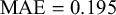 $\text {MAE}=0.195$
. However, while the independent beta fusion models cannot outperform the Turner models in terms of Brier score, the Skill–Difficulty Correlated Fusion Model performs best of all considered fusion models with a Brier score of
$\text {MAE}=0.195$
. However, while the independent beta fusion models cannot outperform the Turner models in terms of Brier score, the Skill–Difficulty Correlated Fusion Model performs best of all considered fusion models with a Brier score of
 $\text {BS}=0.118$
, compared to
$\text {BS}=0.118$
, compared to
 $\text {BS}=0.125$
for the second best model HCTALO by Turner et al. (Reference Turner, Steyvers, Merkle, Budescu and Wallsten2014). Looking at entropy, we also see that the Skill–Difficulty Correlated Fusion Model is less uncertain than the Turner models, but more uncertain than the independent beta fusion models with an entropy of
$\text {BS}=0.125$
for the second best model HCTALO by Turner et al. (Reference Turner, Steyvers, Merkle, Budescu and Wallsten2014). Looking at entropy, we also see that the Skill–Difficulty Correlated Fusion Model is less uncertain than the Turner models, but more uncertain than the independent beta fusion models with an entropy of
 $\text {H}=0.247$
.
$\text {H}=0.247$
.
4. Discussion and conclusion
In this work, we introduced a Bayesian model for combining correlated human forecasts. The model assumes that a forecast provided by a forecaster for some query is dependent on both the forecaster’s properties, which we call their skill, and the query’s properties, which we call its difficulty. Further, we assume that the forecasts provided by different forecasters are correlated because they provide forecasts for the same queries. Accordingly, the proposed Skill–Difficulty Correlated Fusion Model represents the forecasts with a beta distribution conditioned on their truth value with skill parameters specific for each forecaster and difficulty parameters specific for each query. By explicitly modeling the forecasters’ skills as well as the queries’ difficulties, the Skill–Difficulty Correlated Fusion Model can implicitly model the correlation between the forecasts provided by different forecasters. Thus, compared to previous models that assume independence, the new model can better represent human forecasts, which are often correlated (Berger, Reference Berger1985; Hogarth, Reference Hogarth1978; Lichtendahl et al., Reference Lichtendahl, Grushka-Cockayne, Jose and Winkler2022; Wilson and Farrow, Reference Wilson, Farrow, Dias, Morton and Quigley2018; Winkler et al., Reference Winkler, Grushka-Cockayne, Lichtendahl and Jose2019; Wiper and French, Reference Wiper and French1995). Also, it explicitly quantifies the skills of individual forecasters and the difficulties of individual queries and thus allows analyzing and comparing different forecasters independently of the queries their forecasts are provided for or different queries independently of the forecasters who provide their respective forecasts. Having learned the model parameters from observed training data, the Skill–Difficulty Correlated Fusion Model can be used to combine new unseen forecasts provided by different forecasters by inferring the posterior distribution over their truth value. Given that the model assumptions are correct, fusion with the Skill–Difficulty Correlated Fusion Model is normative. Thus, the forecasters’ skills as well as their correlation can be normatively considered for fusion. We emphasize, however, that the model cannot represent arbitrary correlation structures. For example, different subgroups with a specific correlation cannot be modeled (see Section 2 of the Supplementary Material for a detailed discussion of this limitation). The model can only represent correlations that are caused by the forecasters seeing the same queries. In particular, it is restricted to positive correlations. Also, the model can only consider forecasters’ skills that are stable over time and can be learned from training data. Consequently, the fusion rule, like any normative model, is normative only if the observed data are well described by the proposed generative model.
We evaluated the Skill–Difficulty Correlated Fusion Model on a data set consisting of 85 forecasters who each provided forecasts for 180 queries. We compared our model’s fusion performance in terms of Brier score, mean absolute error, and entropy to related Bayesian fusion models, which do not consider correlation (Trick et al., Reference Trick, Rothkopf and Jäkel2023; Turner et al., Reference Turner, Steyvers, Merkle, Budescu and Wallsten2014). While the previously proposed independent beta fusion models (Trick et al., Reference Trick, Rothkopf and Jäkel2023) turned out to be overconfident and therefore outperformed the models proposed by Turner et al. (Reference Turner, Steyvers, Merkle, Budescu and Wallsten2014) in terms of mean absolute error but could not outperform them in terms of Brier score, the Skill–Difficulty Correlated Fusion Model performs best of all compared fusion models according to both mean absolute error and Brier score. In addition, it leads to more uncertain fused forecasts than the independent beta fusion models, shown by a higher entropy. Thus, modeling correlations between forecasters in our Skill–Difficulty Correlated Fusion Model fixes the overconfidence problem of the independent beta fusion models.
For exemplary forecasters and queries, we showed how the Skill–Difficulty Correlated Fusion Model quantifies the forecasters’ and queries’ properties, i.e., their skills and difficulties, and how it fits the forecasting data. However, as seen, for example, in Figure 5(c), our model cannot represent a peak at 0.5 in the histogram of provided forecasts, unless all forecasts are concentrated around 0.5 anyway. This peak or blip in the histogram is called the 50–50 blip and is caused by the forecasters’ high epistemic uncertainty (Bruine de Bruin et al., Reference Bruine de Bruin, Fischbeck, Stiber and Fischhoff2002; Fischhoff and Bruine De Bruin, Reference Fischhoff and Bruine De Bruin1999; Karvetski et al., Reference Karvetski, Olson, Mandel and Twardy2013). If the forecasters have absolutely no knowledge about the truth value of a query, i.e., they have high epistemic uncertainty, they choose 0.5. Even for skilled forecasters, this will happen for quite a few queries, at least if the queries’ topics differ from each other. If the forecasts are predictions of the occurrence of future events, whose outcomes cannot be known yet, the 50–50 blip can even be amplified, because it comprises both the forecasts of people that have absolutely no knowledge, i.e., with high epistemic uncertainty, and the predictions that are explicitly intended to express a probability of 0.5, i.e., with high aleatoric uncertainty (Karvetski et al., Reference Karvetski, Olson, Mandel and Twardy2013). Thus, future work should extend the Skill–Difficulty Correlated Fusion Model to explicitly represent a potential peak of forecasts at 0.5, i.e., the 50–50 blip. This might not only improve the model’s fit to real forecasting data but also further improve the fusion performance due to better modeling of the forecasts.
Supplementary material
The supplementary material for this article can be found at https://doi.org/10.1017/jdm.2026.10035.
Data availability statement
Data availability is not applicable to this article as no new data were created in this study.
Funding statement
This work was supported by the German Federal Ministry of Education and Research (BMBF) in the project IKIDA (Grant No. 01IS20045).
Competing interests
The authors declare none.
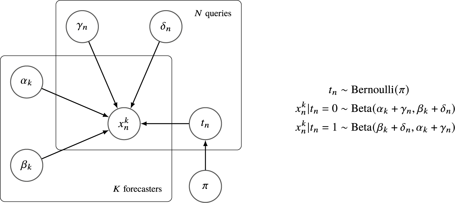


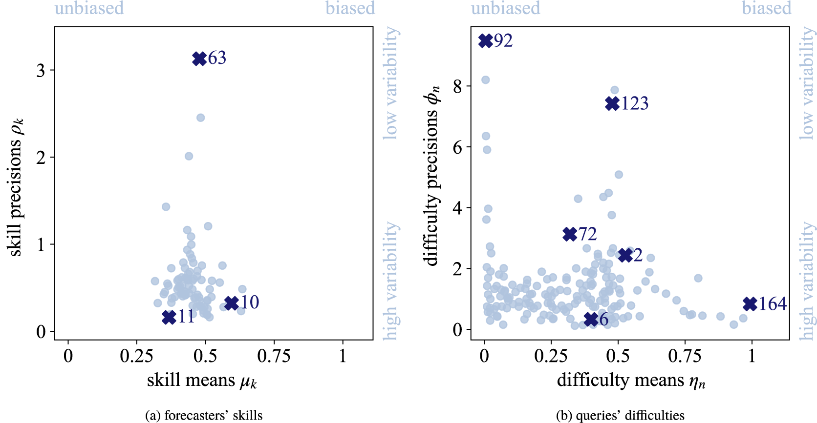


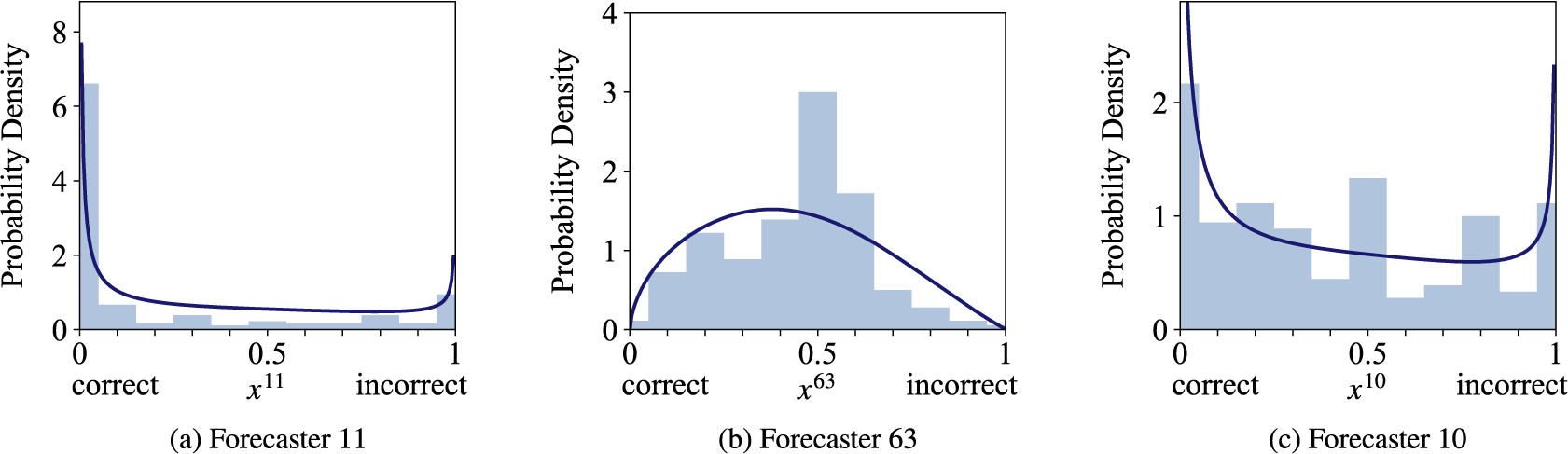


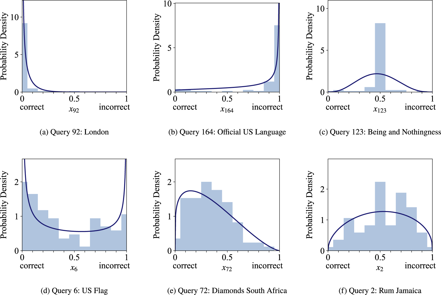


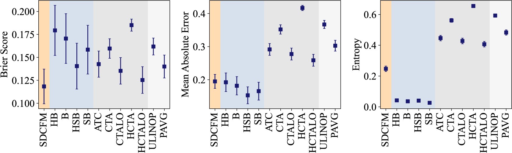


 Open access