





1. Introduction
Failing to correctly adhere to prescribed medication schedules can be extremely harmful to an individual’s health and well-being. However, adherence rates to medication plans are estimated to be only around 50% (Haynes et al., Reference Haynes, McDonald and Garg2002; WHO, 2003). Non-adherence remains a substantial problem even in settings where information and medication are freely available and the costs of failing to adhere are extremely high.Footnote 1 Several behavioral approaches have been proposed to address adherence, but their effectiveness has been mixed (Guinart & Kane, Reference Guinart and Kane2019; Anderson et al., Reference Anderson, Nuckols, Coles, Le, Schnipper, Shane, Jackevicius, Lee and Pevnick2020; Shih & Cohen, Reference Shih and Cohen2020). Two common approaches incentives (see, e.g.DeFulio & Silverman, Reference DeFulio and Silverman2012; Petry et al., Reference Petry, Rash and Byrne2012; Bassett et al., Reference Bassett, Wilson, Taaffe and Freedberg2015) and text-message reminders (see, e.g.Lester et al., Reference Lester, Ritvo, Mills, Kariri, Karanja, Chung, Jack, Habyarimana, Sadatsafavi, Najafzadeh and Marra2010; Pop-Eleches et al., Reference Pop-Eleches, Thirumurthy, Habyarimana, Zivin, Goldstein, De Walque, Mackeen, Haberer, Kimaiyo, Sidle and Ngare2011; Thirumurthy & Lester, Reference Thirumurthy and Lester2012; Mbuagbaw et al., Reference Mbuagbaw, van der Kop, Lester, Thirumurthy, Pop-Eleches, Ye, Smieja, Dolovich, Mills and Thabane2013) typically adopt a “one-size-fits-all” design. Yet, substantial heterogeneity likely exists in both the causes of non-adherence and the effectiveness of interventions. Tailoring interventions to individual characteristics could therefore improve efficiency and reduce costs, but doing so requires a simple and scalable method for identifying those most at risk of low adherence.
This paper investigates whether planning and behavior in a simple, scalable time preference task can predict an individual’s propensity to adhere to prescribed medication. Time preferences vary widely across individuals (see, e.g.Falk et al., Reference Falk, Becker, Dohmen, Enke, Huffman and Sunde2018), and if they are systematically related to adherence, they could serve as a practical diagnostic tool for screening individuals at risk of non-compliance.Footnote 2 Improved identification of adherence risk would be especially valuable for preventive and chronic care, where the benefits of treatment are delayed and non-adherence is difficult to observe directly.
We conduct a low-cost text-message study inviting 694 pregnant South African women to complete a time-preference task and to report adherence to daily iron supplement recommendations for anemia prevention during pregnancy. Because medication adherence is inherently difficult to measure, showing that behavior in a fully observable effort task predicts adherence provides a valuable complement to self-reported measures. Our approach allows us to test whether heterogeneity in time preferences, as reflected in task planning and completion behavior, predicts heterogeneity in medication adherence. This low-cost screening method could help identify individuals who would benefit most from adherence interventions and enable earlier, more efficient targeting - particularly in settings where non-compliance can lead to serious and irreversible health outcomes, such as during pregnancy or in the treatment of HIV or tuberculosis.
Adherence to medication can be viewed as an intertemporal decision problem in which individuals must exert effort today to gain health benefits in the future. Traditional measures of time preference rely on monetary trade-offs between “money now” and “money later” (Andreoni et al., Reference Andreoni, Kuhn and Sprenger2015). However, since adherence involves an “effort now” “benefit later” trade-off, it is more appropriate to measure time preferences in the effort domain (Augenblick et al., Reference Augenblick, Niederle and Sprenger2015; Andreoni et al., Reference Andreoni, Gravert, Kuhn, Saccardo and Yang2018). We therefore implement a simple real-effort task delivered via text message. The design builds on Augenblick et al. (Reference Augenblick, Niederle and Sprenger2015), who use a lab-based effort task to measure time preferences, but we adapt it into a lighter and more scalable version suitable for low-resource environments. Participants are asked to complete a short incentivized word task within a specified number of days in exchange for mobile credit. While the reward and timing of payment are fixed, the difficulty of the task increases with delay, thereby introducing a time–effort trade-off. Before starting, participants also indicate when they plan to complete the task, allowing us to capture both intended and actual behavior.
From this design, we infer two key dimensions: (i) how patient the participant is based on whether she plans to complete the task early or with delay and (ii) whether she behaves as planned, revealing her consistency or potential present bias. Section 3 presents a simple theoretical framework linking time preferences to medication adherence. Section 4 details the experimental design and explains our classification of participants into On-timer, Late-or-Never-Doers, and Early-Doers, based on the timing of task completion relative to their plan. We also distinguish between Early-Planners and Late-Planners according to their initial intentions. Early-Planners can be interpreted as having a higher exponential discount factor  $\delta$, making our classification a noisy but practical proxy for patience. Section 5 outlines the experimental timeline and sample selection.
We find that reported adherence in our sample is high, with most of the 480 women who completed the study reporting daily pill intake (Section 6). Despite limited variation in the outcome, classification as a Late-Planner significantly predicts missed doses, and this measure shows out-of-sample predictive power. Interestingly, about 25% of participants are Early-Doers, 9% are Late-or-Never-Doers, and 66% are On-timers. Given the high share of early completers, we lack power to detect whether deviations from planned timing further predict adherence once planning type is controlled for. Hence, our main result is that planning to do the task on time positively predicts perfect medication adherence. Section 7 explores the robustness of these findings and examines whether they can be explained by demographic characteristics or general busyness of the women.
A related study by John et al. (Reference John and Orkin2022) also uses time-preference elicitation to predict health behavior, in their case, adherence to water chlorination. Unlike our approach, they implement an intensive, in-person intervention to change time preferences, whereas we focus on prediction using a low-touch, remotely delivered diagnostic task. Similarly, Brandt and Dickinson (Reference Brandt and Dickinson2013) find a positive relationship between time preferences and asthma medication adherence, while Mø rkbak et al. (Reference Mørkbak, Gyrd-Hansen and Kjær2017) link present bias to disease onset and prognosis among diabetic patients. Overall, existing evidence is mixed and largely based on small samples or hypothetical measures (Chapman et al., Reference Chapman, Brewer, Coups, Brownlee, Leventhal and Levanthal2001; Sloan et al., Reference Sloan, Padrón and Platt2009; Van Der Pol et al., Reference Van Der Pol, Hennessy and Manns2017)). Our results are consistent with Brandt and Dickinson (Reference Brandt and Dickinson2013) and demonstrate that even a simple classification, based only on when people plan to perform a measurable effort, has significant predictive power for identifying individuals likely to struggle with adherence. This is encouraging for policymakers and health practitioners, as eliciting simple plans is far easier than estimating detailed preference parameters such as  $\delta$ and $\beta$ in the $\beta \delta$-model (O’Donoghue & Rabin, Reference O’Donoghue and Rabin1999).
More broadly, our study contributes to the literature on behavioral interventions to improve medication adherence (see, e.g., Lester et al., Reference Lester, Ritvo, Mills, Kariri, Karanja, Chung, Jack, Habyarimana, Sadatsafavi, Najafzadeh and Marra2010; Pop-Eleches et al., Reference Pop-Eleches, Thirumurthy, Habyarimana, Zivin, Goldstein, De Walque, Mackeen, Haberer, Kimaiyo, Sidle and Ngare2011; Thirumurthy & Lester, Reference Thirumurthy and Lester2012; Bassett et al., Reference Bassett, Wilson, Taaffe and Freedberg2015; Aggarwal et al., Reference Aggarwal, Dizon-Ross and Zuckerin press) and to research on real-effort measurement of time preferences in resource-constrained settings (see, e.g., Augenblick et al., Reference Augenblick, Niederle and Sprenger2015; Andreoni et al., Reference Andreoni, Kuhn and Sprenger2015; Augenblick, Reference Augenblick2018; Augenblick & Rabin, Reference Augenblick and Rabin2019; DellaVigna & Pope, Reference DellaVigna and Pope2018; John et al., Reference John and Orkin2022; Cohen et al., Reference Cohen, Ericson, Laibson and White2020). Together with our findings, this literature highlights the potential of combining scalable behavioral diagnostics with targeted interventions to improve health outcomes and make preventive care more efficient.
2. Context
In this study, we focus on the effect of time preferences on the medication adherence of expectant mothers in South Africa. In 2014, the South African National Department of Health (NDoH) developed a text-message-based information and reminder system called MomConnect. This platform aims to assist expectant mothers through their pregnancy, and in the early period after birth. It does this by, for example, reminding them to schedule pregnancy check-ups, providing them with a description of how babies develop, informing them about the health benefits of breastfeeding, and informing them about symptoms that would indicate that they should seek medical help. When we ran this study, nearly 2 million women had joined MomConnect, making it one of the largest mHealth programs of its kind. Similar programs have been developed in other places, for example in India.
One of the aims of the program is to improve medication adherence among expectant mothers in South Africa, since pregnancy and early infancy are critical periods for the development of a child. In this paper, we focus on studying adherence to the specific recommendation that pregnant women should take daily iron supplements to prevent anemia. Anemia during pregnancy has negative health effects for both mothers and babies. During the last two trimesters of pregnancy, iron is essential for the mother as her body needs to produce more blood and grow both the placenta and the fetus. Anemia is associated with an elevated risk of maternal mortality, problems with lymphocyte stimulation (related to the immune systems), risk of pre-term delivery, and risk of low birth weight (see, e.g.
Allen, Reference Allen2000; Lozoff et al., Reference Lozoff, Beard, Connor, Felt, Georgieff and Schallert2006; Kalaivani, Reference Kalaivani2009; Abu-Saad & Fraser, Reference Abu-Saad and Fraser2010; Balarajan et al., Reference Balarajan, Ramakrishnan, Özaltin, Shankar and Subramanian2011). The World Health Organization estimates that in 2016 the rate of anemia amongst women of reproductive age was around  $25\%$ in South Africa and $33\%$ globally (World Health Organization, 2020). This is in spite of the fact that in South Africa the government runs a program to supply free iron supplements to all pregnant women. Health workers are instructed to provide pregnant woman with a supply of the supplements at the first antenatal visit and to follow-up by checking for signs of anemia during the second visit (for further evidence documenting the status of anemia and iron supplement intake in the South African context, see, e.g.
Nojilana et al., Reference Nojilana, Norman, Dhansay, Labadarios, Van Stuijvenberg and Bradshaw2007; Phatlhane et al., Reference Phatlhane, Zemlin, Matsha, Hoffmann, Naidoo, Ichihara, Smit and Erasmus2016; Tunkyi & Moodley, Reference Tunkyi and Moodley2016; Mbhenyane & Cherane, Reference Mbhenyane and Cherane2017; Harika et al., Reference Harika, Faber, Samuel, Kimiywe, Mulugeta and Eilander2017; Symington et al., Reference Symington, Baumgartner, Malan, Wise, Ricci, Zandberg and Smuts2019).
$33\%$ globally (World Health Organization, 2020). This is in spite of the fact that in South Africa the government runs a program to supply free iron supplements to all pregnant women. Health workers are instructed to provide pregnant woman with a supply of the supplements at the first antenatal visit and to follow-up by checking for signs of anemia during the second visit (for further evidence documenting the status of anemia and iron supplement intake in the South African context, see, e.g.
Nojilana et al., Reference Nojilana, Norman, Dhansay, Labadarios, Van Stuijvenberg and Bradshaw2007; Phatlhane et al., Reference Phatlhane, Zemlin, Matsha, Hoffmann, Naidoo, Ichihara, Smit and Erasmus2016; Tunkyi & Moodley, Reference Tunkyi and Moodley2016; Mbhenyane & Cherane, Reference Mbhenyane and Cherane2017; Harika et al., Reference Harika, Faber, Samuel, Kimiywe, Mulugeta and Eilander2017; Symington et al., Reference Symington, Baumgartner, Malan, Wise, Ricci, Zandberg and Smuts2019).
In summary, all women from whom we sample are recommended to take iron supplements and should have access to free supplements. This makes the context ideal for testing our research question because it enables us to abstract from budget and availability constraints. At the same time, the South African setting is one in which the WHO numbers suggest that there is scope for reducing anemia and where a suitable platform for scalable interventions is well-established.
3. Theoretical framework
In this section, we provide a simple theoretical framework to illustrate the effect of time preferences on the decision to take iron supplements.Footnote 3 The theoretical framework informs our experimental design and the interpretation of our results.
A pregnant woman’s decision of whether to follow the recommendation to take iron supplements daily during pregnancy has similar characteristics to an investment decision: It requires an immediate cost and involves a future benefit. The immediate cost  $c$ includes the effort cost of getting and taking supplements, the cognitive cost of remembering to take the supplements, and costs of short term side effects such as an upset stomach. In general, the cost would also involve costs of buying the supplements but in our setting pills are typically available for free at the health centers. The future benefits $b_t$ capture all health benefits to the mother and her baby, e.g. the reduced risk of maternal mortality, the reduced risk of pre-term delivery, and the reduced risk of low birth weight. If the expectant mothers do not take iron supplements, they receive the best alternative payoff which, without loss of generality, we normalize to $0$.
$0$.
As with other investment decisions, the decision to take daily supplements is an inter-temporal decision problem. Allowing for the present-biased time preferences (Phelps & Pollak, Reference Phelps and Pollak1968; Laibson, Reference Laibson1997; O’Donoghue & Rabin, Reference O’Donoghue and Rabin1999) as captured by the  $\beta \delta-$model (O’Donoghue & Rabin, Reference O’Donoghue and Rabin1999), the net benefit of taking the supplements in period $t$ are:
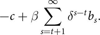 \begin{equation}
-c + \beta \sum_{s=t+1}^{\infty} \delta^{s-t}b_s.
\end{equation}
\begin{equation}
-c + \beta \sum_{s=t+1}^{\infty} \delta^{s-t}b_s.
\end{equation}where  $\beta$ is an additional discount factor between present and future periods, applied on top of the usual exponential discount factor $\delta$. The expectant mother has time-consistent preferences if $\beta=1$ and she has present-biased preferences whenever $\beta \lt 1$. As suggested by O’Donoghue and Rabin (Reference O’Donoghue and Rabin1999) individuals may or may not correctly anticipate future present bias. Let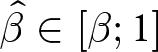 $\hat{\beta}\in[\beta;1]$ denote the prediction of $\beta$ in future periods. The standard time-consistent exponential discounter then has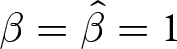 $\beta=\hat{\beta}=1$, the sophisticated present-biased individual has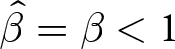 $\hat{\beta}=\beta \lt 1$, and the fully naive present-biased individual has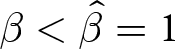 $\beta \lt \hat{\beta}=1$. With this notation the expectant mother anticipates that the future net benefit of doing the task in a future period is $-c + \hat{\beta} \sum_{s=t+1}^{\infty} \delta^{s-t}b_s$. Hence, naive present-biased individuals mispredict their future net benefit. The distinction between naivety and sophistication may be of importance, when individuals have opportunities to delay doing a task (e.g. to later in the day),Footnote 4 as sophisticates will anticipate that they may not do the task if they delay. As shown by O’Donoghue and Rabin (Reference O’Donoghue and Rabin1999), sophisticates may then do the task sooner than a time-consistent individual would have done and they may use commitment devices to ensure that they take supplements. This simple model illustrates a number of ways in which time-preference may influence adherence:
• Adherence is increasing in patience as captured by the exponential discount factor $\delta$, i.e. women who are more impatient and therefore discount the future more are less likely to take supplements.
• For naives, adherence is increasing in the present-bias parameter
$\beta$, i.e. women who display time-inconsistent delay are less likely to take supplements.• Sophistication can alleviate problems related to present-bias.


4. Observing time preferences in the effort domain
We set out to design a simple incentivized time-preference experiment which can be used in low resource settings to classify participants in a meaningful way according to their behavior in the experiment. Our simple task does not allow for tight identification of time preference parameters. Nevertheless, we will demonstrate the usefulness of our categorizations for predicting adherence.
Traditionally, time preferences have been elicited in the monetary domain, where participants choose between either more money now or more money later. However, recent papers have emphasized the importance of measuring time preferences within the specific domain of interest (see, e.g., Ubfal, Reference Ubfal2016; Augenblick et al., Reference Augenblick, Niederle and Sprenger2015; Cohen et al., Reference Cohen, Ericson, Laibson and White2020). Since adhering to medication can be viewed as a type of (cognitive) effort task, we investigate time preferences in the effort domain. For this purpose, we design a simplified version of the experiment used by Augenblick et al. (Reference Augenblick, Niederle and Sprenger2015)Footnote 5 which is suitable for a text-message based implementation.
4.1. Experimental design
The experiment begins on day  $t=0$ when participants are informed that they can earn phone credits worth 20 South African Rand (equivalent to 1.4 USD) if they complete a word task. The task involves writing a list of words backwards. Participants are given two examples and are told that they will receive text messages containing the relevant word lists in the coming days. Importantly, the longer participants wait to do the task, the more words they will need to write to earn the 20 Rand phone credits. The reason for this increasing effort cost is to make procrastination expensive. The participants can choose between writing four words on day $t=1$, six words on day $t=3$, or ten words on day $t=5$. Irrespective of when they complete the task, they will receive phone credits on day $t=7$. At time $t=0$, participants are fully informed about this procedure and are asked whether and when they expect to do the task. We provide a fixed payment of 5 Rand for their answer to this question on day $t=0$ and we do not incentivize how accurately their choice on day $t=0$ matches subsequent choices.
On day  $t=1$, participants receive a new message with a list of four words: “baby, parent, bottle, mom.” A participant who replies with these words written backward has completed the task. If the participant does not complete the task, she gets two additional chances to do the task: on day $t=3$ and on day $t=5$ when new lists of words are sent. The time-line of the text-message task can be seen in Figure 1 and the full set of messages for the task can be found in Appendix.
Timeline of the text-message-based real-effort task

We developed this specific word task for several reasons. First, the task had to be suitable for the text-message implementation. The majority of the effort tasks commonly used in the economics literature are either too long, or infeasible for a limited contact context such as this (e.g. implemented over text-message).Footnote 6 Second, in our setting, it is important that participants can complete the task at any time throughout a day. This way the task might mimic the underlying effort and cognitive constraints that drive time preferences and medication adherence. In pilot tests, we found that although the word task was considered tedious and frustrating, it did not take long to do.
4.2. Interpreting choices in the time-preference elicitation
We follow the approach in Augenblick (Reference Augenblick2018) and Augenblick and Rabin (Reference Augenblick and Rabin2019) to classify time preferences from a comparison of future and immediate effort choices. The initial plan of whether and when to do the task is a future effort choice. Behavior in the subsequent periods, implicitly give us an immediate effort choice. However, the simplicity of our task implies that we cannot identify precise estimates of the time-preference parameters in the  $\beta \delta$-model; instead, we classify the women based on their future effort choice as either Early-Planners (who plan to do the task as soon as possible) or Late-Planners (who plan to delay the task). These two classifications are noisy measures of the participant’s patience as often captured by the exponential discount factor. In addition, we classify the participants based on whether their future and immediate effort choices are consistent meaning that they act according to plan. The women are therefore classified as either On-Timers (who do the task when they had planned), Late-or-Never-Doers (who do the task later than planned if at all) or Early-Doers (who do the task earlier than planned).Footnote 7 We discuss the details of the classifications in the following subsections.
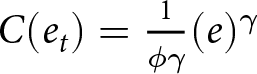
To illustrate the classification mechanism, let  $k$ denote the time period when an effort decision is made, let $t$ denote the time period when the task is performed, and let $e_t$ denote the effort level, i.e. number of written words where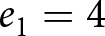 $e_1=4$,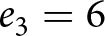 $e_3=6$ and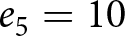 $e_5=10$. The wage level, $w$, is the amount of money paid out at time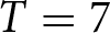 $T=7$. In our experiment, $w =20$ if the participant completes the task at any point in time, and $w=0$ otherwise. For tractability we assume that the disutility of effort is captured by a function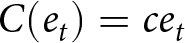 $C(e_t)=ce_t$. We allow for variation in $c$ across individuals and time to capture variation in busyness, distractions, phone access, and salience. We let $c$ have distribution $F(c)$ with mean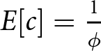 $E[c]=\frac{1}{\phi}$ such that $\phi$ can be interpreted as the expected “exchange rate” between effort and money as in Augenblick (Reference Augenblick2018).Footnote 8 We assume that both effort and monetary payments are discounted by a quasi-hyperbolic discounting function that discounts costs by the discount factor 1 when $t = k$ and $\beta \delta^{t-k}$ when $t \gt k$.
In this setting, where the payment for the task does not depend on when the task is completed, utility maximization is equivalent to effort-cost minimization subject to a participation constraint. The participation constraint ensures that the discounted effort cost of doing the task at the chosen time  $t^*$ does not exceed the discounted payment from doing the task. That is at time $k\geq0$ the participant should expect to do the task at time
 \begin{equation}
t^\star=\underset{t\in\{1,3,5\},t\geq k}{\operatorname{argmin}}\{\beta^{1(k \lt t)}\delta^{t-k}\cdot c_t^{(1-1(k \lt t))}(\frac{1}{\phi})^{1(k \lt t)}e_t\}
\end{equation}
\begin{equation}
t^\star=\underset{t\in\{1,3,5\},t\geq k}{\operatorname{argmin}}\{\beta^{1(k \lt t)}\delta^{t-k}\cdot c_t^{(1-1(k \lt t))}(\frac{1}{\phi})^{1(k \lt t)}e_t\}
\end{equation}subject to the participation constraint  $\beta \delta^{T-k}\cdot 20\geq \beta^{1(k \lt t^\star)} \delta^{{t^\star-k}}\cdot c_{t^\star}^{(1-1(k \lt t^\star))}(\frac{1}{\phi})^{1(k \lt t^\star)}e_{t^\star}$ where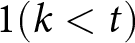 $1(k \lt t)$ is an indicator function for whether the effort allocation is in the future relative to the point in time when the decision is made, and where $c_t$ is the time $t$ realization of $c$ which is only known once period $t$ arrives. In both Equation 2 and in the participation constraint, $\beta$ is replaced by $\hat{\beta}$ when the participant makes a prediction about future present bias. This allows us to capture full sophistication (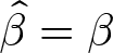 $\hat{\beta}=\beta$), partial sophistication (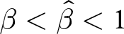 $\beta \lt \hat{\beta} \lt 1$) and naivete (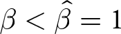 $\beta \lt \hat{\beta}=1$) about future present bias. Below we describe optimal behavior under various assumptions regarding sophistication. We refer to the appendix for the technical details.
4.2.1. Future effort choices: what do women plan to do?
At time  $k=0$ the participant states whether and when she plans to do the task and therefore implicitly states anticipated future effort at time $t=1$, $t=3$ and $t=5$. As mentioned above we do not incentivize the accuracy with which the future effort choice matches effort choices made at later points in time (i.e. for $k \gt 0$). This is to reduce the extent to which (sophisticated) participants use their answer at time $k=0$ as a commitment device to discipline future behavior and it is important because our categorization of individuals is based on a comparison between future and immediate effort choices, and hence to get variation in behavior, we do not specifically want to encourage (or discourage) consistent behavior.
For ease of exposition, we first focus on the case were individuals at time  $k=0$ are naive about future present bias.Footnote 9 That is the women do not foresee that present bias will influence future behavior when they state their plan. This naivete assumption leaves room for discrepancies between planned effort) from the perspective of time $k=0$) and actual behavior (at time $k \gt 0$) even in cases where the realized costs of effort is exactly as expected (i.e.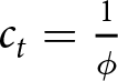 $c_t=\frac{1}{\phi}$).
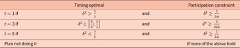
Solving the problem in Equation (2) for  $k=0$ involves doing a number of pairwise comparisons of the discounted cost of exerting effort at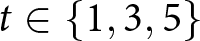 $t\in\{1,3,5\}$. Table 1 summarizes the conditions generated by the pairwise comparisons. Since subjects are making the plan at time $k=0$, all effort costs and payments are in the future. This implies that $\beta$ is irrelevant and cancels out. Furthermore, all effort costs are equal to the expected level an hence choices depend on the exchange rate between effort and money $\phi$ rather than on a specific realization of $c$.
$c$.
Planned future effort
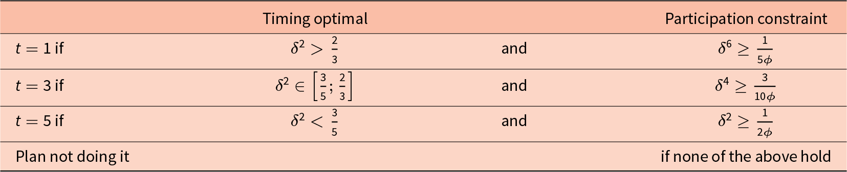
Notes: The table gives conditions under which the alternative possible timings are optimal perspective of period  $k=0$ if individuals are exponential discounters or naively present-biased at $k=0$. Further details are provided in the appendix.
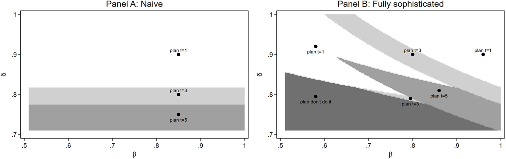
Table 1 clearly shows that a participant may plan not to do the task, if the participation constraints are not satisfied, e.g. because the exchange rate  $\phi$ is such that the wage paid is insufficient. If at least one of the participation constraints hold, then the anticipated optimal timing for the effort only depends on the size of her exponential discount factor, $\delta$. A participant with a low level of patience (i.e. a low $\delta$) will plan to do the task later. Therefore if we assume naivete (or standard exponential discounting at time $k=0$), the plan revealed in the first part of the experiment only depends on the exponential discount factor $\delta$ and not on the present bias parameter $\beta$ or beliefs thereof. This is also illustrated in Panel A of Figure 2.
Model implied planned behavior for different levels of  $\beta$ and $\delta$
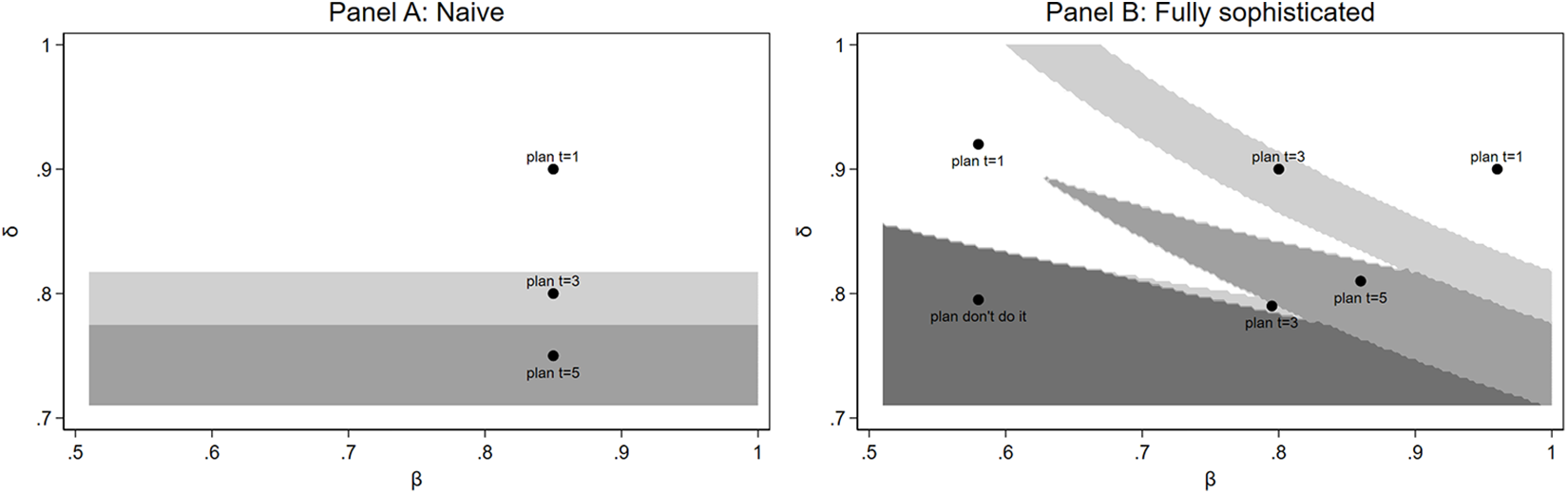
In contrast, if the women are partially or fully sophisticated about their present bias at time  $k=0$, the analysis is somewhat more complicated as the individual then takes into account that even if she would like to complete the task on a particular day from the perspective of time $k=0$, when she arrives at that particular day, she may procrastinate due to her present bias. An individual who is fully sophisticated at time $k=0$ will realize this and will therefore estimate when she will actually do the task (if at all) and she will adjust her plan accordingly. In order, to make her plan, she will therefore solve the problem backwards and start by considering what she would expect to do if she arrives at the last period and has not yet done the task. Will it then be optimal to do the task? Or will she expect not to do the task? Given expected behavior in the last period, what is then optimal behavior in the period before that, etc.? This implies that the plan made by fully or partial sophisticates at time $k=0$ depends not only on $\delta$ but also on $\hat{\beta}$ since expected behavior at time $t\geq1$ depends on both $\delta$ and $\hat{\beta}$. Panel B of Figure 2 illustrates planned behavior in this case for fully sophisticated women (who have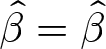 $\hat{\beta}=\hat{\beta}$). For partial sophisticates, the $\beta$ on the horizontal axis is simply replaced by $\hat{\beta}$ and planned behavior then depends on the belief about $\beta$ rather than the actual underlying preference parameter. The figure shows that even when women are fully sophisticated at time $k=0$, it is the case, that for high or low values of $\beta$, those women who plan to do the task at time $t=1$ have a higher exponential discount rate $\delta$ than those who plan to do the task later at $t\geq3$. For intermediate values of $\beta$ there is a less clear association between planning to do it early and $\delta$.
Nevertheless, under our assumptions, our model suggests that individuals who plan to do the task early in period  $t=1$ (illustrated by the white areas in Figure 2) often have a high exponential discount factor $\delta$. We therefore classify participants based on their planned behavior as either Early-Planners if they plan to do the task in period $t=1$ or as Late-Planners otherwise (illustrated by the gray shaded areas in Figure 2)Footnote 10 and use this as a noisy classification of how much the participants discount the future. Late-Planners who plan to delay the task to period $t\geq3$ are largely less patient and discount more, hence their exponential discount factor $\delta$ is lower than that of Early Planners who plan to perform the task immediately in period $t=1$.
4.2.2. Future versus immediate effort choices: do women act according to plan?
The second part of our classification of behavior involves comparing the time  $k=0$ plan of future effort to immediate effort choices made in periods $k=1$, $k=3$ and $k=5$, in order to elicit possible inconsistencies between the plan and actual behavior. Solving for the optimal timing in Equation (2) for $k=\{1,3,5\}$ again involves doing a number of pairwise comparisons in order to determine if planned behavior still is optimal as time progresses, and if it is not what the women will do instead. Within our model there are two basic components which may lead to deviations from planned behavior. First, when faced with a particular task, the individual may experience effort costs that are higher or lower than expected. That is, the realization of $c_t$ may differ from $E(c_t)$. If the effort costs are higher than expected, the woman may (regardless of their time preferences) choose to postpone the task and vice versa if the effort costs are lower than expected. In section 7, we discuss the extent to which systematic variation in effort costs may have influenced our findings. However, to ease the exposition in this subsection we will assume that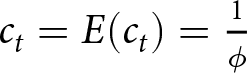 $c_t=E(c_t)=\frac{1}{\phi}$ for all $t$ meaning that there is no time variation in effort cost. This is clearly a simplification but it enables us to focus on the second component of the model, which can result in deviations from planned behavior: present bias. In our analysis, we allow for naivete, as well as both full and partial sophistication, and we consider these cases in turn.
A fully sophisticated women with 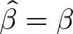 $\hat\beta=\beta$, will do exactly as planned when we abstract from variation in effort costs. This is because these women fully understand the extent of their present bias and therefore perfectly adjust their plan to reflect their subsequent behavior.
In contrast, a present-biased naive individual with 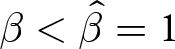 $\beta \lt \hat{\beta}=1$ plans as if she has no present bias, but once the time to do a task arrives she will be influenced by her present bias and if the present-bias is strong enough she may want to delay the effort. Panel A of Figure 3 illustrates the theoretical predictions of planned and actual behavior for different combinations of the parameters $\delta$ and $\beta$ for navies.Footnote 11. Along the vertical axis the figure mirrors Panel A of 2 and shows that for navies planned behavior is determined only by the size of $\delta$ as discussed in the previous subsection. Actual behavior in contrast depends on both $\beta$ and $\delta$. The very light gray areas indicate that the task is carried out as planned. Purple areas indicate that the task is carried out with delay which can occur if the women have intermediate level present-biased preferences. The blue shaded areas indicate situations where individuals plan to do the task but fail to do it. This can happen if the women have strongly present-biased preferences ( $\beta \lt 1$) and a relatively low exponential discount factor ( $\delta$).
Model implied planned and actual behavior for different levels of  $\beta$ and $\delta$
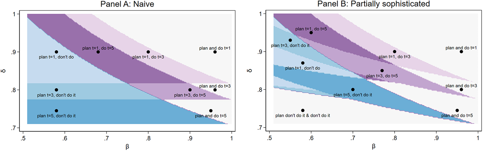
The behavior of partial sophisticated individuals is illustrated in Panel B of Figure 3 where we have set 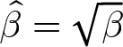 $\hat\beta=\sqrt\beta$ which ensures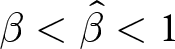 $\beta \lt \hat\beta \lt 1$. We use the same color coding. Clearly, compared to naifs, there are more combinations of $\beta$ and $\delta$ where women behave as they said they would (light gray areas). But unlike for the fully sophisticated, there are also cases where the women delay the task longer than planned (purple areas) or fail to do it even though they had planned to do the task (blue areas).
We group participants in our experiment along the color code as the colors represent different behaviors that can serve as noisy measures of underlying time preferences:
• On-timers: These individuals carry out the task as planned (as in the light gray areas of the figure) and fully sophisticated women. Our model suggests that these women either have time-consistent preferences or only slightly present-biased preferences (
$\beta$ close to one) or they are sufficiently sophisticated about their present bias to be able to carry out their initial plan. In addition, the effort cost of doing the task does not deviate too much from what they had expected.• Late-or-never-doers: These women do the task later than planned, if at all (represented by the blue or purple areas above). Our model suggests that these are women who are present biased and to some extent naive, such that they fail to carry out their initial plan. However, this group also includes individuals who may in fact have limited self-control problems but for whom the effort cost of doing the task turns out to be much greater than expected.
• Early-doers: These are women who are either future biased or face a lower effort cost than expected.

5. Implementation and sample selection
The data collection took place from the 19 March to the 29 June 2019. In total, a sample of 18,400 women was drawn randomly from the population of MomConnect users. We used the following criteria: (i) on the 19 March 2019, there were between 105 and 130 days until their expected due date, and (ii) the women were aged 18 or older. We sampled from the entire country and did not place a restriction on language. We have information on their preferred language, whether they live in an urban or rural area and whether they signed up with a smart phone or an older mobile phone without smart-phone capabilities.
This sample of women received a text-message invitation in English 105 days prior to their estimated due date asking whether they would like to participate in a research study on healthy pregnancy behavior for which they could earn phone credits. In line with our pre-study expectations, approximately 24% (4226) of the contacted women opted in to participate.Footnote 12 These women were then randomized into six different treatment arms that were run in parallel. In total, 694 of the women were randomly assigned to the treatment arm relevant for the current paper.
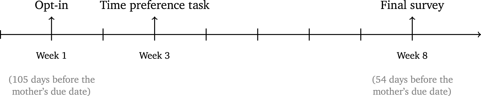
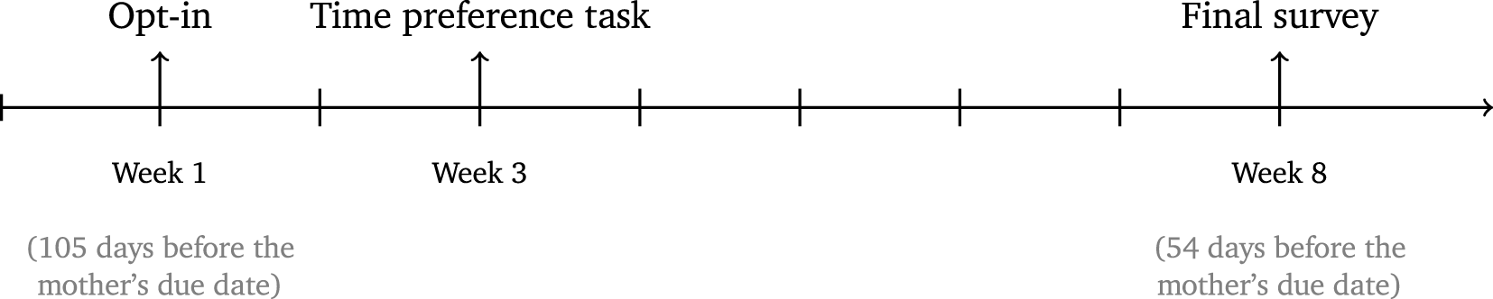
A timeline of their participation can be seen in Figure 4. In an initial survey, participants were asked some baseline questions, including how many older children they had and whether they thought iron supplements were important for a healthy mother and child.Footnote 13 Fifteen days after opting in to the study, the women received the instructions for the real-effort time-preference task of writing words backwards. A total of 546 participants took part in the time-preference task. Approximately five weeks later, in the final week of data collection for this study, the women were asked to complete a short survey consisting of eight questions including questions about iron intake, iron deficiency and symptoms, perceived difficulty of remembering to take iron supplements, and experienced side effects.Footnote 14
Timeline of the experiment
For our main analysis, we limit our sample to women who took part in the time-preference task and answered all eight questions of the final survey. This leaves us with a final sample of 480 women.Footnote 15 Table C.7 in Appendix C reports some basic demographic information for the individuals in our final sample. The average woman was born in 1992, making her 27 years old at the time of our data collection. Thirty-five percent of our sample has English as their preferred language. Twenty-nine percent of the women live in urban areas and on average the participants have one older child and 12 years of schooling. The table also tests whether there is biased selection on observables into our final analysis sample. Compared to the full sample of women who opted in, our final sample shows a slightly lower share of urban women. Otherwise, there are no observable differences.
6. Results
6.1. Behavior in the time-elicitation task
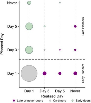
Among the 480 women in our final sample, 333 (70%) reported that they planned to do the task on the first day, while 69 (14%) and 63 (13%) women answered that they would wait and do it on day 3 or 5, respectively. Fifteen women (3%) stated that they did not plan to do the task. In practice, 432 (90%) of the women actually did the task on the first day.Footnote 16 This implies that a large fraction of our sample (121 women) actually did the task earlier than they had planned. However, the majority of women (301 participants) performed the task as planned. Only 43 of our participants did the task later than planned or not at all, despite having stated that they would do it.
As discussed in section 4.2.1 and section 4.2.2 we use this behavior to classify the women in two ways. First, we classify women into Early-Doers, Late-Doers and On-Timers. Second, we classify the women as being either Early or Late Planners based on when they planned to do the task. Individuals that planned to do the task on day 1 are called “Early Planners”, while everyone else is labeled “Late Planners”. Figure 5 reports the distribution of women according to the categorizations, showing the On-Timers in grey, the Early-Doers in green and the Late-Doers in purple and Early Planners below the dashed line while Late Planners are those above the dashed line.
Categorization
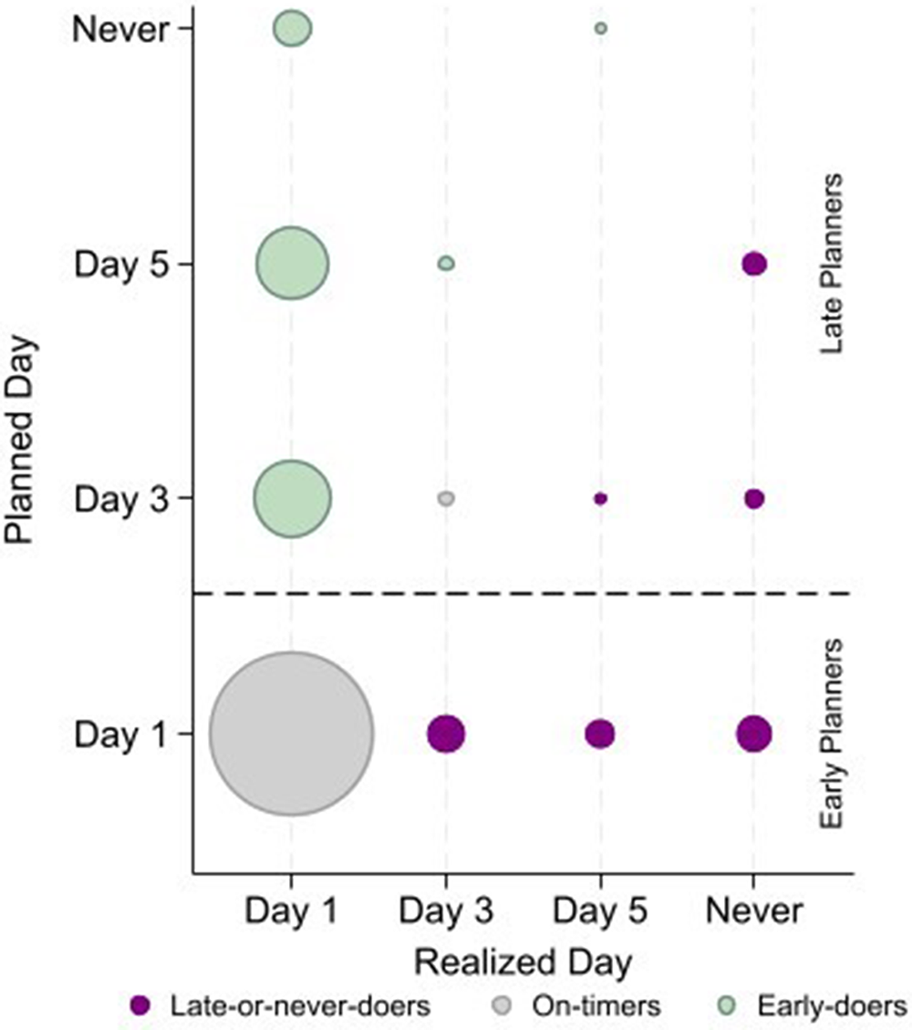
By construction, an individual cannot be classified as both an Early Planner, planning to do the task on the first day, and an Early-Doer, doing it earlier than planned. Since many of our participants ended up doing the task on the first day, 136 out of 147 Late Planners are classified as Early-Doers, so the Late Planners and Early-Doer groups are nearly overlapping. Therefore, we focus on both the Late Planners and the Late-Doers in our empirical analysis.
6.2. Self-reported adherence
Our main outcome variable is self-reported adherence. The variable is measured in response to the question: “How many days did you take your iron pills last week? (1-7)”. We ask about the past week, rather than about the entire pregnancy, because imperfect and motivated recall becomes more of an issue when asking individuals to report outcomes from a longer time window.Footnote 17 However, it is important to keep in mind that even when considering the shorter period of a week, taking an iron pill on a particular day may not be a particularly memorable moment, and self-reported medication adherence should therefore be seen as a proxy for actual adherence. In addition, research suggests that self-reported estimates tend to be upward biased due to social desirability bias (Wilson et al., Reference Wilson, Carter and Berg2009). However, self-stated measures of medication adherence are widely used in the literature and have been found to correlate strongly with objective measures.Footnote 18 This suggests that the over-reporting shifts the measured distribution of adherence to the right, but remains informative regarding the relative adherence of different individuals (i.e. regarding who adheres more and who adheres less). Further, evidence from Barron et al. (Reference Barron, Damgaard and Gravert2026) indicates that women in this study population report adherence honestly. In that analysis, self-reported adherence correlated sensibly with external factors: women who reported that free pills were unavailable at their clinic were less likely to report full adherence, and adherence was positively associated with recent doctor visits but negatively with being told they had low iron levels. Reports of adherence were also highly consistent across two survey rounds 17 days apart. Additional checks in Barron et al. (Reference Barron, Damgaard and Gravert2026) showed that reporting low iron, an easily recalled outcome, was predicted by difficulty remembering to take pills, side effects, and fatigue, and negatively associated with knowledge and beliefs about iron. These relationships are as expected, supporting the credibility of women’s self-reports. As this paper uses a random subsample from the same population, we rely on those findings as evidence of honest reporting here.
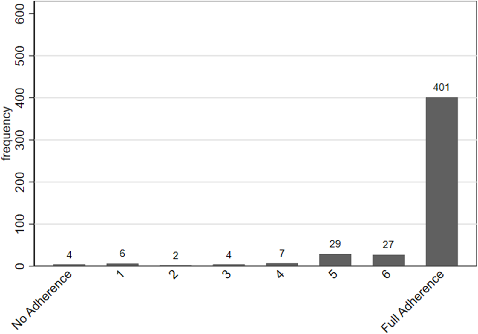
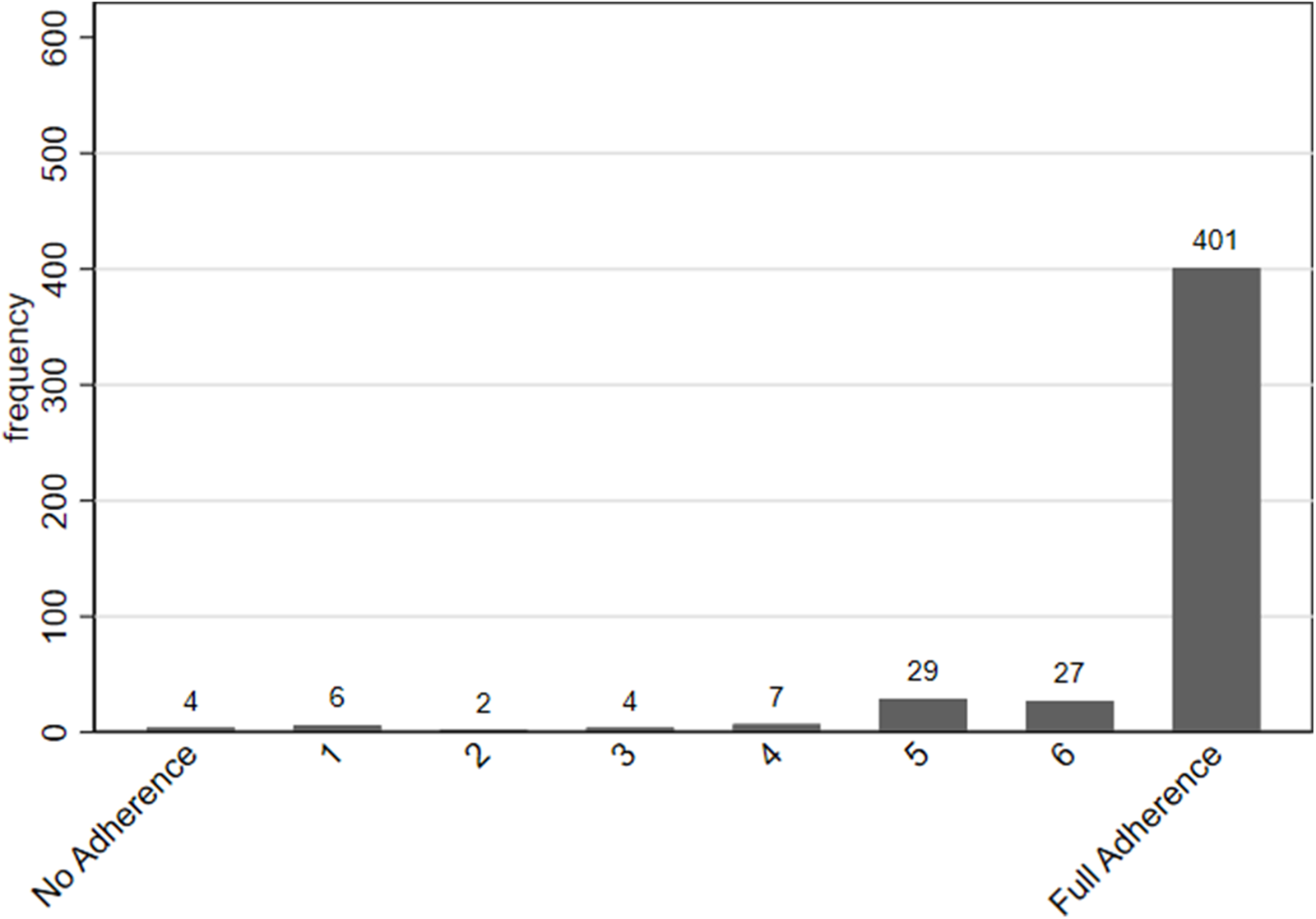
Figure 6 reports the distribution of self-reported adherence, showing that individuals in our sample tended to show a high degree of adherence to their iron supplements, with only 79 out of 480 reporting that they did not take their iron pills every day during the preceding week.
Iron intake last week
6.3. The relationship between the discount factor and adherence
The central question that we ask in this paper is whether we can use elicited time preferences from an extremely simple, low-cost, real-effort task to predict which individuals will be more likely to adhere to their iron supplements.
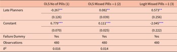
Our model suggests that self-reported adherence is increasing in the discount factor  $\delta$, i.e. women who discount future effort more are more likely to delay and therefore less likely to take their supplements. We investigate this question in Table 2. The first column reports the results from an OLS regression, showing the relationship between the number of pills taken during the last week and whether an individual is classified as an Late Planner according to our time-preference task.Footnote 19 In line with the model intuition, we find that Late Planners take fewer pills than Early Planners, with results significant at the 5% level. Since the key distinction in adherence behavior appears to be between full adherence (i.e. taking the pills on all seven days) and partial adherence (i.e. taking pills on fewer than seven days), we also construct a binary variable that reflects whether an individual missed an iron pill on at least one day, or not. Replacing the continuous outcome variable with this binary outcome variable, columns 2 (OLS) and 3 (Logit), shows that Late Planners are more likely to be partial adherers.
Adherence of late planners
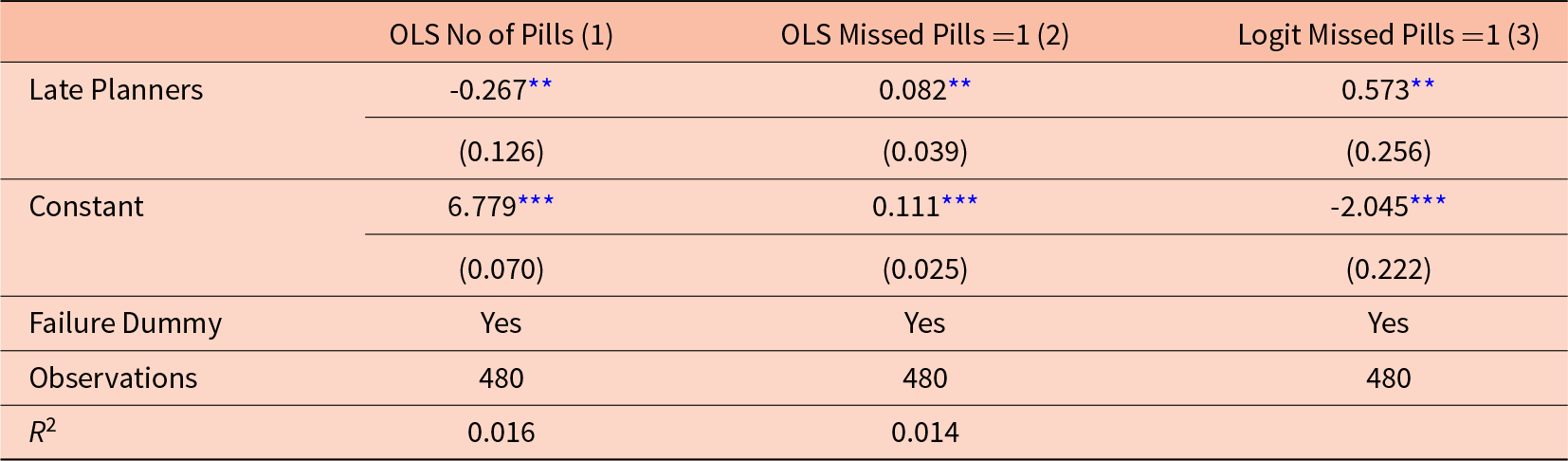
Notes: Regressions include the 480 participants that answered all eight questions of the final survey. Missed Pills =1 is a dummy variable which is 0 if the participant reported having taken all 7 pills last week, and which is 1 if she missed one pill or more. Late Planners is a dummy variable where planning to do the task on day 1 is denoted 0 and planning to do the task on day 3 or 5, or not planning to do the task is denoted with a 1. Failure Dummy is a dummy for technical problems leading to payment delay. Regressions include the 480 participants that answered all eight questions of the final survey. Robust standard errors in parentheses
*** p  $ \lt 0.01$, ** p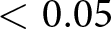 $ \lt 0.05$, * p $ \lt 0.1$.
Being a Late Planner is therefore significantly correlated with not fully adhering to the prescribed medication plan. We conducted several exercises to test the robustness of this result to the inclusion of additional covariates. Table C.11 in Appendix C reports these results and shows that the estimates are robust to adding a measure of self-reported risk aversion, controlling for the respondent’s language, and controlling for their education level. The results are also robust when excluding participants who did not plan to do the task at all (see Table C.12 in the Appendix).
6.4. The relationship between time-consistency and adherence
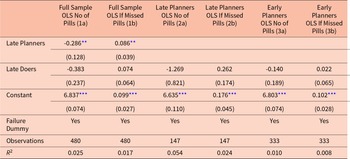
Our model further suggests that adherence is lower for individuals who display time-inconsistent delay. Table 3 examines the relationship between adherence behavior and discounting, including our classification of individuals as Late-Doers. Columns 1a and b show that the effect for Late Planners shown above is robust to the inclusion of the Late-Doer dummy. In addition, the point estimates for the Late-Doers dummy are consistent with the intuition that people who plan to do the time-preference task early, but then procrastinate or fail to do it, take fewer pills and are more likely to have missed a pill. However, these effects are neither significant in regressions for the full sample, nor in regressions using the sub-samples of Late and Early Planners, respectively (see columns 2a, 2b, 3a, and 3b). One potential explanation for the lack of significance is the unanticipated low degree of variation in the outcome variable, which reduced the power of our analysis.
Planning, doing and adherence
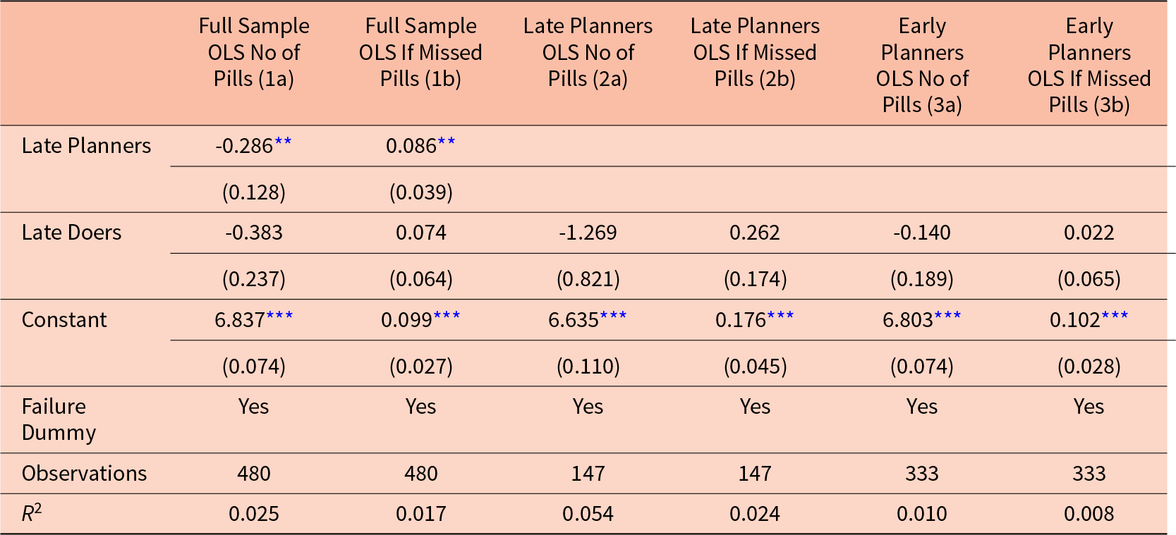
Notes: Results in column 1a and 1b are shown for the 480 participants who have done the full survey and use the full information on all attempts to do the task at any of the possible days. Column 2a-2b and 3a-3b show results using the subsamples of Late Planners and Early Planners, respectively. Late Planners is a dummy variable where planning to do the task on day 1 is denoted 0 and planning to do the task on day 3 or 5, or not planning to do the task is denoted with a 1. Late doers are people who planned to do the word task sooner, did it later or did not do it. Missed Pills = 1 is a dummy variable which is 0 if the participant reported having taken all 7 pills last week. OLS Regressions. Robust standard errors in parentheses
*** p $ \lt 0.01$, ** p $ \lt 0.05$, * p $ \lt 0.1$.
6.5. The predictive power of our classifications
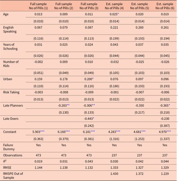
We have now established that our classifications have the expected sign, even if the effect is not always statistically significant. We now investigate whether our classifications have predictive power beyond that provided by usual demographic variables, that might be used by policy makers to classify individuals. We do this both within and out-of sample. First we estimate a benchmark prediction model, where we predict adherence (“Number of Pills”) using other individual characteristics: age, language, years of schooling, number of previous children, living area, and a risk taking measure (column 1 of Table 4).Footnote 20
Prediction analysis: Number of pills taken
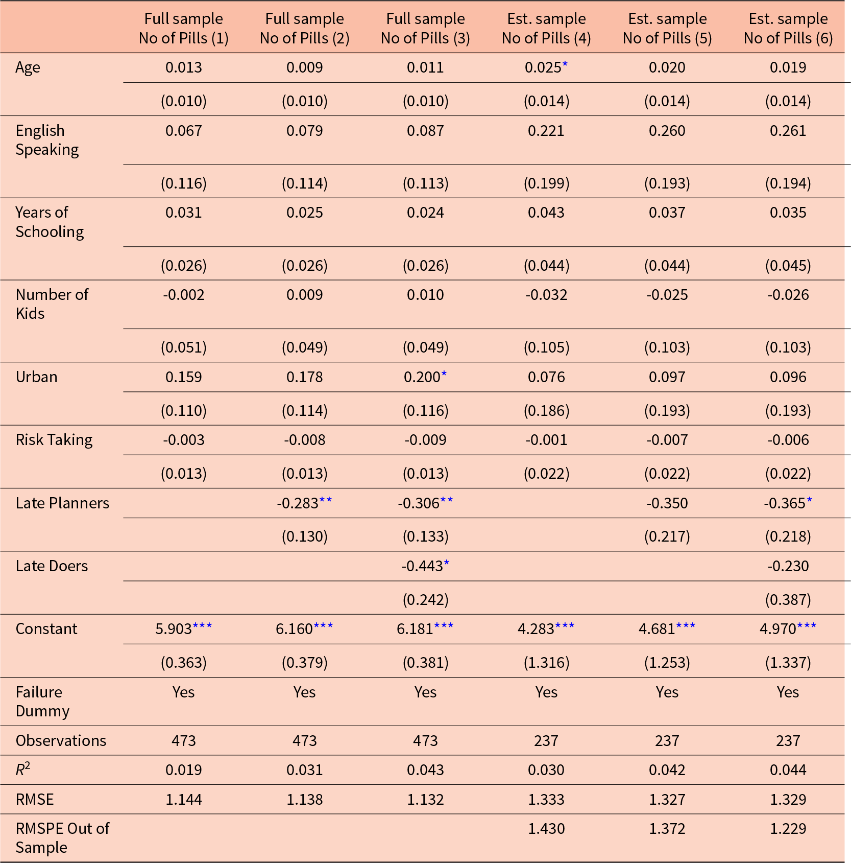
Notes: The full sample include the 473 participants that answered all eight questions of the final survey and for whom all controls are available. 7 observations are dropped because we lack information on the number of kids. The estimation sample excludes a hold-out sample consisting of the 50% of women who are due last. RMSE and RMSPE are the Root Mean Square Error corrected for degrees of freedom of the estimation and hold-out sample respectively. Robust standard errors in parentheses.
*** p  $ \lt 0.01$, ** p $ \lt 0.05$, * p $ \lt 0.1$.
We find that basic demographics do not correlate in a meaningful way with medication adherence. However, when we add our classifications, we confirm our findings from the previous section and also improve our Root Mean Squared Error (RMSE), showing that the classifications have predictive power.
In columns 4-6 of Table 4 we repeat this analysis but estimate the model using only 50% of the sample of the estimation while the remaining 50% are left as a hold-out sample for out-of-sample prediction. The hold-out sample consists of women with the latest due dates. The estimated coefficients for our time-preference measures are again of similar magnitude, but in this exercise we clearly lose statistical power. Nevertheless, adding our measure of Late Planners still leads to a small improvement in RMSE and adding both time-preference measures improves the out-of-sample Root Mean Squared Prediction Error (RMSPE).
Hence, we show that our task provides predictive power that goes beyond using simple demographics to classify the women.
7. Are the women simply busy?
One question that might come to mind is whether our results are driven by time preferences or simply by the fact that some women are busier or more distracted than others. In our theoretical model, we allow effort costs to vary over time and over individuals. It may be the case that our simple time-preference task is providing a measurement of how busy and cognitively constrained mothers are in their everyday lives, as opposed to being a “clean” measure of time preferences.
To investigate this, we approximate busyness in three ways. First, throughout their pregnancy, the mothers receive multiple messages as part of the larger experiment which they are asked to respond to. One might expect that women who are busier, in general, would take a longer time to answer these messages. Second, the timing of messages depends on the individual estimated due date of each expectant mother. Since the women have different due dates that are as good as random, they receive the same message on different days of the week. This provides us with exogenous variation in which day of the week a given message is received. We can use this variation to examine the role of being busy under the assumption that busyness varies between weekdays and the weekend. Lastly, it is plausible that women who already have kids at home might be busier than those who are pregnant with their first child. We use each of these three measures of busyness to provide evidence about whether busyness is a central mechanism driving our results.
First, we examine how quickly the expectant mothers replied to other messages, unrelated to the time-preference task. At the end of the first week after signing up for the study, participants received an incentivized text message asking them to reply with the first 4 digits of their ID number. This was nine days before the time-preference task and the purpose of the question was to see if the participant was still actively engaged and responsive to the study.Footnote 21 Table C.14 in Appendix C shows that there is no correlation between answering the text message in the first hour or not answering at all, and on the other hand, when they planned to do or actually did the time-preference task. We take this as evidence that our time-preference task is not driven by a general state of being busy when receiving the texts.Footnote 22
Second, we examine whether the day-of-the week of receiving the message informing them about the time-reference task influenced their anticipated or actual behavior in the task. For some women, day 1 falls on a Friday, day 3 on a Sunday, and day 5 on a Tuesday. If a woman is less busy on weekends, then she might decide to do the task on Sunday (i.e on day 3), thus looking like a Late Planner to us. However, Table C.15 in Appendix C investigates if there is any difference in planning or completion of the task, depending on the day the task was received. Table C.15 shows no significant differences in the day-of-the-week in any of the results of the time-reference task, indicating that this is not a major concern in this setting.
Third, we replicate our regressions from Table 2, but now include “number of kids” as a control (see Tables C.16) The “number of kids” variable is not significant and does not change the estimates.
Overall, these results indicate that individual heterogeneity in general “busyness” of expectant mothers is not the primary driver of our results. We cannot control for all sources of busyness or exogenous shocks, so there might be some unobserved factors, but those women, who have no time or interest in taking part in our study should have already selected out of the sample at the start. Nevertheless, participation of those who opted in was very high and very consistent across several weeks.
8. Conclusion
In recent years, health care has shifted toward prevention rather than treatment (CDC, 2009). Preventing illness is both more effective and less resource intensive than managing disease after onset. While medical research increasingly emphasizes genetic markers and biomarkers to forecast disease susceptibility, behavioral science offers complementary tools for predicting and influencing health behaviors, especially for conditions driven by behavioral rather than purely genetic factors. From a policy perspective, improving the ability to anticipate and modify health behavior before problems arise represents an important step toward better health outcomes and reduced long-term costs.
This study demonstrates that time preferences, elicited through a simple real-effort task, correlate with medication adherence. Because adherence is difficult to observe and often relies on self-reporting, showing that behavior in a fully measurable experimental task can predict adherence offers a valuable diagnostic alternative. In a field study of 480 pregnant women in South Africa, we find that this low-cost and easily implemented measure predicts self-reported adherence even in a population with limited variation in reported adherence. Women who delay completing the task are less likely to adhere fully to their medication regimen, and those who fail to complete it as planned are also less likely to take daily iron supplements. Our results also show that demographic variables, such as location, age, and number of children, provide limited predictive power, despite being common criteria for targeting health interventions.
Kini and Ho (Reference Kini and Ho2018) highlight a range of strategies to improve adherence, from patient education to reminders and incentives, but note concerns about scalability and cost. A practical way to address these challenges is to improve screening so that interventions focus on those most at risk of non-adherence. Better prediction of adherence enables more precise targeting, reducing unnecessary interventions, participant fatigue, and welfare losses from commitment devices (Bai et al., Reference Bai, Handel, Miguel and Rao2021). Traditional nudges tend to apply uniformly, often achieving modest effects of only 2–8% (DellaVigna & Linos, Reference DellaVigna and Linos2022). Combining behavioral diagnostics with targeted interventions could substantially enhance their impact, as suggested by Campos-Mercade et al. (Reference Campos-Mercade, Meier, Schneider and Wengström2021), who show that experimentally measured prosociality predicts adherence to health recommendations during a pandemic.
Behavioral diagnostics have already proven useful in optimizing incentive contracts for health workers in Pakistan (Callen et al., Reference Callen, Andreoni, Khan, Jaffar and Sprenger2023). Extending such approaches to patients offers a scalable and low-cost method to predict and improve adherence, particularly in low-resource settings where mHealth systems such as MomConnect and similar platforms in India or Kenya already exist. In our sample, simply distinguishing between early and late planners predicted adherence weeks later, suggesting that a straightforward diagnostic measure can yield policy-relevant insights.
While precise estimates of parameters like  $ \delta $ and $ \beta $ remain valuable for theory, the policy relevance of preference-based diagnostics depends on their simplicity and interpretability. This paper is a first step toward developing more targeted and cost-effective behavioral interventions based on individual characteristics such as patience. Our highly motivated sample of pregnant women posed a challenge for both variation in outcomes as well as for observing present bias and should thus be interpreted as a lower limit of predictability. Future research should test this approach across diverse health contexts and populations and compare it with direct self-reported intentions to adhere to treatment to find the most cost-effective method to predict adherence.
Supplementary material
The supplementary material for this article can be found at https://doi.org/10.1017/esa.2025.10027.
Acknowledgements
The authors are grateful to the Praekelt Foundation and the South African National Department of Health (NDoH) for collaborating with us. Funding was generously provided by Trygg-Hansas Forskningsfond, Sweden. The activities of CEBI are financed by the Danish National Research Foundation, Grant DNRF134. The AEA RCT Registry trial number associated with this project is AEARCTR-0004018. Ethics Approval has been obtained from Pharma Ethics Ltd, Reference No:181021588. The authors have no conflict of interest.









 Open access

