


1. Introduction
Solving a linear DSGE model is often the first step in analyzing a structural macroeconomic question. A key computational challenge is solving the associated matrix quadratic equation efficiently and accurately. Existing methods, such as the generalized Schur (QZ) decomposition (Moler and Stewart, Reference Moler and Stewart1973) are widely used but can struggle with computational efficiency and scalability for large-scale models or when iteratively exploring multiple parameterizations. We demonstrate the potential of Structure-Preserving Doubling Algorithms (SDA)Footnote 1 to overcome these challenges by applying them to two practical contexts: first, in Smets and Wouters’s (Reference Smets and Wouters2007) New Keynesian model, where we evaluate performance across varying monetary policy rules; and second, in a comprehensive comparison using 142 models from the Macroeconomic Model Data Base (MMB).Footnote 2 In both cases, SDAs outperform conventional methods in terms of speed and accuracy, particularly when refining solutions or solving large models.
Doubling algorithms are certainly not unknown to economists (see, e.g., Hansen and Sargent, Reference Hansen and Sargent2014, Chapter 3.6). Anderson and Moore (Reference Anderson and Moore1979) consider doubling algorithms to solve the Riccati equations occurring in optimal linear filtering exercises. Building on this, Anderson et al. (Reference Anderson, McGrattan, Hansen and Sargent1996, Section 10, p. 224) use doubling algorithms to receive a conditional log-likelihood function for linear state space models (see also Harvey, Reference Harvey1990, Chapter 3, p. 119, 129). Furthermore, McGrattan (Reference McGrattan1990) as well applies doubling algorithms to the Riccati and Sylvester equations in the unknown matrices of the linear solution to LQ optimal control problems in economics. As our class of models as defined by Dynare (Adjemian et al. 2011) (henceforth Dynare) includes and expands on this class of models, our approach here can be seen as an extension, specifically to Anderson et al. (Reference Anderson, McGrattan, Hansen and Sargent1996) work.Footnote 3 More closely related is the application to Riccati equations (see Poloni (Reference Poloni2020) for an accessible introduction to doubling algorithms for Riccati equations), a link between the solution of Riccati equations and the matrix quadratic we solve is noted explicitly by Higham and Kim (Reference Higham and Kim2000) and Bini et al. (Reference Bini, Meini and Poloni2008), for example—both are quadratic equations in a matrix unknown, but with different structures. Chiang et al. (Reference Chiang, Chu, Guo, Huang, Lin and Xu2009), however, present explicit results for matrix polynomials with doubling methods—specifically structure preserving doubling methods, see Huang et al. (Reference Huang, Li and Lin2018)—and connect these algorithms to reduction algorithms (Latouche and Ramaswami’s (Reference Latouche and Ramaswami1993) logarithmic and Bini and Meini’s (Reference Bini and Meini1996) cyclic) that are algorithms available in Dynare,Footnote 4 though arguably undocumented.Footnote 5 Beyond relating these algorithms using unified notation, we provide iterative capabilities (i.e., updating or refining some initialized solution) using Bini and Meini (Reference Bini and Meini2023) that allow us to operate on a starting value for a solution to the matrix quadratic for the first SDA, First Standard Form (SF1). We show, however, that while this may reduce the computation time, the asymptotic solution of the second SDA, Second Standard Form (SF2), is unaffected.
We engage in a number of experiments to compare the algorithms to QZ-based methods,Footnote 6 Dynare’s implementation of Latouche and Ramaswami’s (Reference Latouche and Ramaswami1993) logarithmic reduction algorithm and Bini and Meini’s (Reference Bini and Meini1996) cyclic reduction algorithms, Meyer-Gohde and Saecker’s (Reference Meyer-Gohde and Saecker2024) Newton algorithms, and Meyer-Gohde’s (Reference Meyer-Gohde2025) Bernoulli methods following the latter’s experiments to ensure comparability. We begin by comparing the methods in the Smets and Wouters (Reference Smets and Wouters2007) model of the US economy—at the posterior mode, a numerically problematic calibration, and in solving for different parameterizations of the Taylor rule. In the latter, we move through a grid of different values of the reaction of monetary policy to inflation and output. Whereas the QZ and reduction methods have to recalculate the entire solution at each new parameter combination, the iterative implementations of the SDA like Newton and Bernoulli algorithms can initialize using the solution from the previous, nearby parameterization. As the parameterizations get closer together, the advantage in terms of computation time increases significantly, while the accuracy (measured by Meyer-Gohde’s (Reference Meyer-Gohde2023) practical forward error bounds) remains unaffected. We show that one of the doubling algorithms profits from this effect, while the other does not—this is consistent with our theoretical results that this particular doubling algorithm converges to the same solution regardless of its initialization.
We then compare the different methods using the models in the MMB, both initializing with a zero matrix (as implied by Latouche and Ramaswami’s (Reference Latouche and Ramaswami1993) logarithmic reduction and Bini and Meini’s (Reference Bini and Meini1996) cyclic reduction algorithms) and as solution refinement for iterative implementations (i.e., initializing the iterative methods with the QZ solution). We find that the reduction and doubling methods provide useable alternatives to the standard QZ.Footnote 7 The cyclic reduction algorithm suffers from unreliable convergence to the stable solution and the doubling algorithms perform more reliably than both the reduction methods, providing higher accuracy at frequently lower cost than alternatives including QZ. While each of the two doubling algorithms have their relative advantages as unconditional methods, one is particularly successful at solution refinement. This algorithm, consistent with the grid experiment in the Smets and Wouters (Reference Smets and Wouters2007) model, reliably provides large increases in accuracy at low additional computation costs—exactly what would be demanded of such an algorithm.
2. Problem statement
Standard numerical solution packages for DSGE models such as Dynare analyze models that can generally be collected in the following nonlinear functional equation
 \begin{align} &0 = E_t [f(y_{t+1}, y_t, y_{t-1}, \varepsilon _t)] \end{align}
The function
 $f \,:\, \mathbb{R}^{n_y}\times \mathbb{R}^{n_y}\times \mathbb{R}^{n_y}\times \mathbb{R}^{n_e}\rightarrow \mathbb{R}^{n_y}$
comprises the conditions (first-order conditions, resource constraints, market clearing, etc.) that characterize the model; the endogenous variables
$f \,:\, \mathbb{R}^{n_y}\times \mathbb{R}^{n_y}\times \mathbb{R}^{n_y}\times \mathbb{R}^{n_e}\rightarrow \mathbb{R}^{n_y}$
comprises the conditions (first-order conditions, resource constraints, market clearing, etc.) that characterize the model; the endogenous variables
 $y_t\in \mathbb{R}^{n_y}$
; and the exogenous shocks
$y_t\in \mathbb{R}^{n_y}$
; and the exogenous shocks
 $\varepsilon _{t}\in \mathbb{R}^{n_e}$
, where
$\varepsilon _{t}\in \mathbb{R}^{n_e}$
, where
 $n_y,n_e\in \mathbb{N}$
and
$n_y,n_e\in \mathbb{N}$
and
 $\varepsilon _{t}$
has a known mean zero distribution. The solution to the model (1) is the unknown function
$\varepsilon _{t}$
has a known mean zero distribution. The solution to the model (1) is the unknown function
 \begin{align} y_t = y(y_{t-1}, \varepsilon _t),\quad y \,:\,\mathbb{R}^{n_y+n_e}\rightarrow \mathbb{R}^{n_y} \end{align}
that maps states,
 $y_{t-1}$
and
$y_{t-1}$
and
 $\varepsilon _t$
, into endogenous variables,
$\varepsilon _t$
, into endogenous variables,
 $y_t$
. A closed form for (2) is generally not available and we must approximate. One point in the solution, the deterministic steady state
$y_t$
. A closed form for (2) is generally not available and we must approximate. One point in the solution, the deterministic steady state
 $\overline {y}\in \mathbb{R}^{n_y}$
such
$\overline {y}\in \mathbb{R}^{n_y}$
such
 $\overline {y}=y(\overline {y}, 0)$
and
$\overline {y}=y(\overline {y}, 0)$
and
 $0 = f(\overline {y}, \overline {y}, \overline {y}, 0)$
, can often be solved for and this provides a point around which local solutions can be expanded.
$0 = f(\overline {y}, \overline {y}, \overline {y}, 0)$
, can often be solved for and this provides a point around which local solutions can be expanded.
The linear, or first-order, approximation of (1) at the steady state gives
 \begin{align} 0=A E_t [y_{t+1}]+B y_t+C y_{t-1} +D\varepsilon _t \end{align}
where
 $A$
,
$A$
,
 $B$
,
$B$
,
 $C$
, and
$C$
, and
 $D$
are the derivatives of
$D$
are the derivatives of
 $f$
in (1) evaluated at the steady state and the
$f$
in (1) evaluated at the steady state and the
 $y$
’s in (3) now, reusing notation, are the (log) deviations of the endogenous variables from their steady states,
$y$
’s in (3) now, reusing notation, are the (log) deviations of the endogenous variables from their steady states,
 $\overline {y}$
. The solution to (3) is a linear solution of the form (2)
$\overline {y}$
. The solution to (3) is a linear solution of the form (2)
 \begin{align} y_t = P\;y_{t-1}+ Q\;\varepsilon _t \end{align}
which expresses
 $y_t$
as a function of its own past,
$y_t$
as a function of its own past,
 $y_{t-1}$
, and the shocks,
$y_{t-1}$
, and the shocks,
 $\varepsilon _t$
.
$\varepsilon _t$
.
Substituting (4) into (3) and recognizing that
 $E_t\left [\varepsilon _{t+1}\right ]=0$
yields the following
$E_t\left [\varepsilon _{t+1}\right ]=0$
yields the following
 \begin{align} 0&=A P^2+B P+C,\;\;\;\;0=\left (A P+B\right )Q+D \end{align}
The former is quadratic with potentially multiple solutions—generally a
 $P$
with all its eigenvalues inside the open unit circle is sought. As Lan and Meyer-Gohde (Reference Lan and Meyer-Gohde2014) prove, the latter can be uniquely solved for
$P$
with all its eigenvalues inside the open unit circle is sought. As Lan and Meyer-Gohde (Reference Lan and Meyer-Gohde2014) prove, the latter can be uniquely solved for
 $Q$
if such a
$Q$
if such a
 $P$
can be found, our focus will be the former, the unilateral quadratic matrix equations (UQME). In the following we show how to solve for
$P$
can be found, our focus will be the former, the unilateral quadratic matrix equations (UQME). In the following we show how to solve for
 $P$
in (5) using SDAs.
$P$
in (5) using SDAs.
3. Doubling methods for linear DSGE models
In this section, we outline two SDAs, well known from the applied mathematics literature (e.g. Huang et al. Reference Huang, Li and Lin2018), and apply them to solve linear DSGE models. While the algorithms themselves are not new, we contribute by showing how to recast the UQME (5) into the standard forms—First Standard Form (SF1) and Second Standard Form (SF2)—required to apply these methods. We establish a link between the standard conditions used in the DSGE literature to ensure existence and uniqueness of a solution and the convergence requirements of SDAs, as discussed in Section 4. Finally, we present extensions of both algorithms to incorporate an initial guess to enable them to act as refinement tools in iterative applications.Footnote 8
3.1 Matrix quadratics, pencils, and doubling
We begin by expressing the UQME in (5) as a subspace problem via the first companion linearization of the matrix quadratic problem (Hammarling et al. Reference Hammarling, Munro and Tisseur2013)
 \begin{align} \mathscr{A} \mathscr{X} = \mathscr{B} \mathscr{X} \mathscr{M} \end{align}
with
 \begin{align*} \mathscr{X}= \begin{pmatrix} I \\ P \end{pmatrix} && \mathscr{A}= \begin{pmatrix} 0 &\quad I \\ C &\quad B \end{pmatrix}, && \mathscr{B}= \begin{pmatrix} I &\quad 0\\ 0 &\quad -A \end{pmatrix}, && \mathscr{M}=P \end{align*}
Clearly, any
 $P$
satisfying (5) is a solution of (6). Further, the eigenvalues of
$P$
satisfying (5) is a solution of (6). Further, the eigenvalues of
 $\mathscr{M}$
are a subset of the generalized eigenvalues of the matrix pencil
$\mathscr{M}$
are a subset of the generalized eigenvalues of the matrix pencil
 $\mathscr{A}-\lambda \mathscr{B}$
, i.e.,
$\mathscr{A}-\lambda \mathscr{B}$
, i.e.,
 $\operatorname {eig}(\mathscr{M})\subset \operatorname {eig}(\mathscr{A},\mathscr{B})$
.
$\operatorname {eig}(\mathscr{M})\subset \operatorname {eig}(\mathscr{A},\mathscr{B})$
.
We make the standard assumption in the literature for the existence of a unique stable solvent
 $P$
, i.e., Blanchard and Kahn (Reference Blanchard and Kahn1980) celebrated rank and order conditions.
$P$
, i.e., Blanchard and Kahn (Reference Blanchard and Kahn1980) celebrated rank and order conditions.
Assumption 1 (Blanchard and Kahn (Reference Blanchard and Kahn1980) Rank and Order). There exist
-
(1)
 $2n_y$
latent roots of
$A\lambda ^2+B\lambda +C$
(
$n_y+\mathrm{rank}\left (A\right )$
finite
$\lambda \in \mathbb{C}:\det {(A\lambda ^2+B\lambda +C)} = 0$
and
$n_y-\mathrm{rank}\left (A\right )$
“infinite”
$\lambda$
) with
$n_y$
inside or on and
$n_y$
outside the unit circle.
$2n_y$
latent roots of
$A\lambda ^2+B\lambda +C$
(
$n_y+\mathrm{rank}\left (A\right )$
finite
$\lambda \in \mathbb{C}:\det {(A\lambda ^2+B\lambda +C)} = 0$
and
$n_y-\mathrm{rank}\left (A\right )$
“infinite”
$\lambda$
) with
$n_y$
inside or on and
$n_y$
outside the unit circle.
-
(2) a
$P\in \mathbb{R}^{n_y\times n_y}$
with
$\rho (P)\leq 1$
that satisfies the primary matrix quadratic
where
\begin{equation*}0=A P^2+B P+C\end{equation*}
$\rho (X)$
denotes the spectral radius of a matrix
$X$
.


The quadratic convergence of our SDAs requires the existence of a unique solvent to the reverse problem, which follows directly from Assumption 1.Footnote 9
Corollary 1 (Solvent of the Dual Matrix Equation). Let Assumption
1
hold. There exists a
 $P_d\in \mathbb{R}^{n_y \times n_y}$
with
$P_d\in \mathbb{R}^{n_y \times n_y}$
with
 $\rho (P_d)\lt 1$
that satisfies the dual matrix quadratic
$\rho (P_d)\lt 1$
that satisfies the dual matrix quadratic
 \begin{equation*}0=C P_d^2+B P_d+A.\end{equation*}
The problem in (6) is an eigenvalue problem and can thus be solved numerically using the QZ or generalized Schur decomposition of Moler and Stewart (Reference Moler and Stewart1973). In the online appendix, we derive the solution with QZ by working directly with the linear algebraic problem. This should link the more familiar QZ with the doubling algorithms we will subsequently present more clearly to readers looking for additional intuition.
We will approach the matrix pencil problem here via a doubling approach. In detail we will try to generate sequences
 $\{\mathscr{A}_k\}_{k=1}^N$
and
$\{\mathscr{A}_k\}_{k=1}^N$
and
 $\{\mathscr{B}_k\}_{k=1}^N$
such that
$\{\mathscr{B}_k\}_{k=1}^N$
such that
 \begin{align} \mathscr{A}_k \mathscr{X} = \mathscr{B}_k \mathscr{X} \mathscr{M\,}^{2^k} \end{align}
squaring the matrix
 $\mathscr{M}$
in each iteration. At the same time, we will seek to preserve the structure of the pencil, e.g., a special block structure of
$\mathscr{M}$
in each iteration. At the same time, we will seek to preserve the structure of the pencil, e.g., a special block structure of
 $\mathscr{A}_k$
and
$\mathscr{A}_k$
and
 $\mathscr{B}_k$
. This will enable us to express the algorithm in terms of submatrices of
$\mathscr{B}_k$
. This will enable us to express the algorithm in terms of submatrices of
 $\mathscr{A}_k$
and
$\mathscr{A}_k$
and
 $\mathscr{B}_k$
instead of the matrices in their entirety and makes sure that we can repeat the doubling step in the next iteration.
$\mathscr{B}_k$
instead of the matrices in their entirety and makes sure that we can repeat the doubling step in the next iteration.
Following Guo et al. (Reference Guo, Lin and Xu2006), a transformation
 $\,\,\,\,\widehat{\!\!\!\!\mathscr{A}}-\lambda \,\,\widehat {\!\!\mathscr{B}}$
of a pencil
$\,\,\,\,\widehat{\!\!\!\!\mathscr{A}}-\lambda \,\,\widehat {\!\!\mathscr{B}}$
of a pencil
 $\mathscr{A}-\lambda \mathscr{B}$
is called a doubling transform if
$\mathscr{A}-\lambda \mathscr{B}$
is called a doubling transform if
 \begin{align} \,\,\,\,\widehat{\!\!\!\!\mathscr{A}}=\overline {\mathscr{A}}\mathscr{A},\;\;\;\;\,\,\widehat {\!\!\mathscr{B}}=\overline {\mathscr{B}}\mathscr{B} \end{align}
for
 $\overline {\mathscr{A}}$
and
$\overline {\mathscr{A}}$
and
 $\overline {\mathscr{B}}$
that satisfy
$\overline {\mathscr{B}}$
that satisfy
 \begin{align} \text{rank}\left (\begin{bmatrix} \overline {\mathscr{A}} &\quad \overline {\mathscr{B}}\end{bmatrix}\right )=2n_y,\;\;\;\;\begin{bmatrix} \overline {\mathscr{A}}&\quad \overline {\mathscr{B}}\end{bmatrix}\begin{bmatrix} \mathscr{B}\\-\mathscr{A}\end{bmatrix}=0 \end{align}
That is, we will be transforming the problem here as in QZ, seeking a structure that is amenable to doubling instead of the upper triangularity sought there.
Such a doubling transformation is eigenspace preserving and eigenvalue squaring (“doubling”) following Guo et al. (Reference Guo, Lin and Xu2006, Theorem 2.1) or Huang et al. (Reference Huang, Li and Lin2018, Theorem 3.1) that we repeat here adapted to our problem
Theorem 1 (Doubling Pencil). Suppose
 $\,\,\,\,\widehat{\!\!\!\!\mathscr{A}}-\lambda \,\,\widehat {\!\!\mathscr{B}}$
is a doubling transformation of the pencil
$\,\,\,\,\widehat{\!\!\!\!\mathscr{A}}-\lambda \,\,\widehat {\!\!\mathscr{B}}$
is a doubling transformation of the pencil
 $\mathscr{A}-\lambda \mathscr{B}$
. Then, as
$\mathscr{A}-\lambda \mathscr{B}$
. Then, as
 $\mathscr{A} \mathscr{X} = \mathscr{B} \mathscr{X} \mathscr{M}$
it follows from (
6
) that
$\mathscr{A} \mathscr{X} = \mathscr{B} \mathscr{X} \mathscr{M}$
it follows from (
6
) that
 \begin{align} \widehat{\!\!\!\!\mathscr{A}} \mathscr{X} = \,\,\widehat {\!\!\mathscr{B}} \mathscr{X} \mathscr{M\,}^2 \end{align}
Proof. See Huang et al. (Reference Huang, Li and Lin2018, Theorem 3.1)
Following this theorem, we obtain a doubling algorithm for (6) by iterating on
 \begin{align} \underbrace {\,\,\,\,\widehat{\!\!\!\!\mathscr{A}}_{k}}_{\mathscr{A}_{k+1}}=\overline {\mathscr{A}}_{k}\mathscr{A}_{k},\;\;\;\;\underbrace {\,\,\widehat {\!\!\mathscr{B}}_{k}}_{\mathscr{B}_{k+1}}=\overline {\mathscr{B}}_{k}\mathscr{B}_{k} \end{align}
initializing with
 $\mathscr{A}$
and
$\mathscr{A}$
and
 $\mathscr{B}$
, as
$\mathscr{B}$
, as
 $\mathscr{A}\mathscr{X}=\mathscr{B}\mathscr{X}\mathscr{M}$
then gives
$\mathscr{A}\mathscr{X}=\mathscr{B}\mathscr{X}\mathscr{M}$
then gives
 \begin{align} \mathscr{A}_{1}\mathscr{X}&=\mathscr{B}_{1}\mathscr{X}\mathscr{M\,}^2&&\rightarrow & \mathscr{A}_{2}\mathscr{X}&=\mathscr{B}_{2}\mathscr{X}\mathscr{M\,}^4&&\rightarrow & \mathscr{A}_{k}\mathscr{X}&=\mathscr{B}_{k}\mathscr{X}\mathscr{M\,}^{2^k} \end{align}
We seek a structure in
 $\mathscr{A}$
and
$\mathscr{A}$
and
 $\mathscr{B}$
such that we calculate
$\mathscr{B}$
such that we calculate
 $\mathscr{A}_{k}\rightarrow \mathscr{A}_{k+1}$
and
$\mathscr{A}_{k}\rightarrow \mathscr{A}_{k+1}$
and
 $\mathscr{B}_{k}\rightarrow \mathscr{B}_{k+1}$
by recursions in elements (here we will settle for submatrices). In the following subsections, we provide two recursions of exactly this structure. Both require that we rearrange our pencil
$\mathscr{B}_{k}\rightarrow \mathscr{B}_{k+1}$
by recursions in elements (here we will settle for submatrices). In the following subsections, we provide two recursions of exactly this structure. Both require that we rearrange our pencil
 $\mathscr{A}-\lambda \mathscr{B}$
to conform to a specific structure of each recursion, as we now show.
$\mathscr{A}-\lambda \mathscr{B}$
to conform to a specific structure of each recursion, as we now show.
3.2 First Standard Form
To obtain the first SDA, we will transform the pencil
 $\mathscr{A}-\lambda \mathscr{B}$
. Assuming that
$\mathscr{A}-\lambda \mathscr{B}$
. Assuming that
 $B$
is non-singular, we receive the primal problem in SF1
$B$
is non-singular, we receive the primal problem in SF1
 \begin{align} \mathscr{A}_0 \mathscr{X} = \mathscr{B}_0 \mathscr{X} \mathscr{M} \end{align}
by multiplying (6) from the left by
 $S$
, where
$S$
, where
 \begin{align*} \mathscr{A}_0 &= \begin{pmatrix} E_0 &\quad 0 \\ -X_0 &\quad I \end{pmatrix}\,:\!=\,S\mathscr{A}, &\quad \mathscr{B}_0 &\quad = \begin{pmatrix} I &\quad -Y_0 \\ 0 &\quad F_0 \end{pmatrix}\,:\!=\,S\mathscr{B}, &\quad S &\quad = \begin{pmatrix} I &\quad -B^{-1}\\ 0 &\quad B^{-1} \end{pmatrix} \end{align*}
Note that (6) and (13) are equivalent in the sense that the pencils
 $\mathscr{A}-\lambda \mathscr{B}$
and
$\mathscr{A}-\lambda \mathscr{B}$
and
 $\mathscr{A}_0-\lambda \mathscr{B}_0$
share the same set of generalized eigenvalues, i.e.,
$\mathscr{A}_0-\lambda \mathscr{B}_0$
share the same set of generalized eigenvalues, i.e.,
 $\operatorname {eig}(\mathscr{A},\mathscr{B})=\operatorname {eig}(\mathscr{A}_0,\mathscr{B}_0)$
. We now use doubling transformations to arrive at a SDA for SF1, computing
$\operatorname {eig}(\mathscr{A},\mathscr{B})=\operatorname {eig}(\mathscr{A}_0,\mathscr{B}_0)$
. We now use doubling transformations to arrive at a SDA for SF1, computing
 $\{{\mathscr{A}}_{k}\}_{k=0}^{\infty }$
,
$\{{\mathscr{A}}_{k}\}_{k=0}^{\infty }$
,
 $\{{\mathscr{B}}_{k}\}_{k=0}^{\infty }$
with
$\{{\mathscr{B}}_{k}\}_{k=0}^{\infty }$
with
 \begin{align} \mathscr{A}_{k+1}&= \begin{pmatrix} E_{k+1} &\quad 0 \\ -X_{k+1} &\quad I \end{pmatrix} \,:\!=\, \begin{pmatrix} E_k\left (I-Y_k X_k \right )^{-1} &\quad 0\\ -F_k\left (I-X_k Y_k\right )^{-1} X_k &\quad I \end{pmatrix} \mathscr{A}_{k} \\[-12pt] \nonumber \end{align}
 \begin{align} \mathscr{B}_{k+1}&= \begin{pmatrix} I &\quad -Y_{k+1} \\ 0 &\quad F_{k+1} \end{pmatrix} \,:\!=\, \begin{pmatrix} I &\quad -E_k\left (I-Y_k X_k \right )^{-1} Y_k \\ 0 &\quad F_k\left (I-X_k Y_k\right )^{-1} \end{pmatrix} \mathscr{B}_{k} \\[6pt] \nonumber \end{align}
such that
 \begin{align} \mathscr{A}_k \mathscr{X} = \mathscr{B}_k \mathscr{X} \mathscr{M\,}^{2^k} \end{align}
A key feature here is that (16) retains SF1 for all
 $k\in \mathbb{N}$
. Algorithm 1 with an initial guess
$k\in \mathbb{N}$
. Algorithm 1 with an initial guess
 $P_0=0$
summarizes this SDA for the SF1. The intuition here is that under some fairly general preconditions, e.g., Assumption 1, the term
$P_0=0$
summarizes this SDA for the SF1. The intuition here is that under some fairly general preconditions, e.g., Assumption 1, the term
 $\mathscr{B}_k \mathscr{X} \mathscr{M\,}^{2^k}$
on the right-hand side of (16) converges to zero for
$\mathscr{B}_k \mathscr{X} \mathscr{M\,}^{2^k}$
on the right-hand side of (16) converges to zero for
 $k\rightarrow \infty$
, so that consequently
$k\rightarrow \infty$
, so that consequently
 $X_k$
converges to
$X_k$
converges to
 $P$
.
$P$
.
A disadvantage of SDAs is that numerical inaccuracies can propagate through iteration if, say, the matrices to be inverted are not well-conditioned. In the context of discrete algebraic Riccati equations (DAREs), Mehrmann and Tan (Reference Mehrmann and Tan1988) show that such a defection of the approximate solution again satisfies a DARE. As a result, after solving a DARE, one can solve the associated DAREs of the approximation error to increase the overall accuracy. Following this, Bini and Meini (Reference Bini and Meini2023) show how to incorporate an initial guess to SDA for the SF1 by means of an equivalence transformation of the pencil
 $\mathscr{A}-\lambda \mathscr{B}$
. Huang et al. (Reference Huang, Li and Lin2018) discuss similar transformations for algebraic Riccati equations (AREs) in general. We introduce such an initial guess by transforming the eigenvalue problem (6) to
$\mathscr{A}-\lambda \mathscr{B}$
. Huang et al. (Reference Huang, Li and Lin2018) discuss similar transformations for algebraic Riccati equations (AREs) in general. We introduce such an initial guess by transforming the eigenvalue problem (6) to
 \begin{align} \,\,\,\,\widehat{\!\!\!\!\mathscr{A}}\, \,\,\,\widehat {\!\!\!\mathscr{X}}\, = \,\,\widehat {\!\!\mathscr{B}}\, \,\,\,\widehat {\!\!\!\mathscr{X}}\, \mathscr{M} \end{align}
with
 $P_0$
as the initial guess such that
$P_0$
as the initial guess such that
 $P=\widehat {P}+P_0$
and
$P=\widehat {P}+P_0$
and
 \begin{align*} \,\,\,\widehat {\!\!\!\mathscr{X}}\, \,:\!=\, \begin{pmatrix} I \\ \hat {P} \end{pmatrix} && \,\,\,\,\widehat{\!\!\!\!\mathscr{A}}\, \,:\!=\, \mathscr{A} \begin{pmatrix} I &\quad 0 \\ P_0 &\quad I \end{pmatrix}, && \,\,\widehat {\!\!\mathscr{B}}\, \,:\!=\, \mathscr{B} \begin{pmatrix} I &\quad 0 \\ P_0 &\quad I \end{pmatrix} \end{align*}
Assuming that
 $B+AP_0$
has full rank, we multiply
$B+AP_0$
has full rank, we multiply
 $\,\,\,\,\widehat{\!\!\!\!\mathscr{A}}$
and
$\,\,\,\,\widehat{\!\!\!\!\mathscr{A}}$
and
 $\,\,\widehat {\!\!\mathscr{B}}$
by
$\,\,\widehat {\!\!\mathscr{B}}$
by
 \begin{align*} \widehat {S}= \begin{pmatrix} \left (B+AP_0\right )^{-1}B &\quad -\left (B+AP_0\right )^{-1}\\ I-\left (B+AP_0\right )^{-1}B &\quad\left (B+AP_0\right )^{-1} \end{pmatrix} \end{align*}
to receive the corresponding problem in SF1, i.e.,
 \begin{align} \,\,\,\,\widehat{\!\!\!\!\mathscr{A}}_0\, \,\,\,\widehat {\!\!\!\mathscr{X}}\, = \,\,\widehat {\!\!\mathscr{B}}_0\, \,\,\,\widehat {\!\!\!\mathscr{X}}\, \mathscr{M} \end{align}
with
 \begin{align*} \,\,\,\,\widehat{\!\!\!\!\mathscr{A}}_0\, &= \begin{pmatrix} \widehat {E}_0 &\quad 0 \\ -\widehat {X}_0 &\quad I \end{pmatrix} \,:\!=\, \widehat {S}\,\,\,\,\widehat{\!\!\!\!\mathscr{A}}, &\quad\hat {\mathscr{B}}_0\, &= \begin{pmatrix} I &\quad -\widehat {Y}_0 \\ 0 &\quad \widehat {F}_0 \end{pmatrix} \,:\!=\, \widehat {S}\,\,\widehat {\!\!\mathscr{B}} \end{align*}
Algorithm 1 summarizes the SDA for SF1 based on an initial
 $P_0$
. Note that a good
$P_0$
. Note that a good
 $P_0$
should increase the probability that
$P_0$
should increase the probability that
 $B+AP_0$
is well-conditioned, since under Assumption 1 we know that
$B+AP_0$
is well-conditioned, since under Assumption 1 we know that
 $B+AP$
has full rank (see Lan and Meyer-Gohde, Reference Lan and Meyer-Gohde2014). In comparison to
$B+AP$
has full rank (see Lan and Meyer-Gohde, Reference Lan and Meyer-Gohde2014). In comparison to
 $P_0=0$
above which is only applicable for non-singular
$P_0=0$
above which is only applicable for non-singular
 $B$
, Algorithm 1 can handle a singular
$B$
, Algorithm 1 can handle a singular
 $B$
, provided we have a
$B$
, provided we have a
 $P_0$
such that
$P_0$
such that
 $B+AP_0$
is non-singular.Footnote
10
$B+AP_0$
is non-singular.Footnote
10
Structure-Preserving Doubling Algorithm (SF1)

3.3 Second Standard Form
Alternatively, Chiang et al. (Reference Chiang, Chu, Guo, Huang, Lin and Xu2009) use a doubling algorithm on the eigenvalue problem
 \begin{align} {\mathscr{A\,\,}}^{\dagger }_0 {\mathscr{X\,\,}}^{\dagger } = {\mathscr{B\,}}^{\dagger }_0 {\mathscr{X\,\,}}^{\dagger } \mathscr{M} \end{align}
with
 \begin{align*} {\mathscr{X\,\,}}^{\dagger }&= \begin{pmatrix} I \\ AP \end{pmatrix}, & {\mathscr{A\,\,}}^{\dagger }_0 &= \begin{pmatrix} {E}^{\dagger }_0 &\quad 0 \\ -{X}^{\dagger }_0 &\quad I \end{pmatrix}\,:\!=\, \begin{pmatrix} -C &\quad 0 \\ 0 &\quad I \end{pmatrix}, &{\mathscr{B\,}}^{\dagger }_0&= \begin{pmatrix} -{Y}^{\dagger }_0 &\quad I \\ -{F}^{\dagger }_0 &\quad 0 \end{pmatrix}\,:\!=\, \begin{pmatrix} B &\quad I \\ A &\quad 0 \end{pmatrix}, \mathscr{M}=P \end{align*}
which satisfies the so-called Second Standard Form (SF2). Again any
 $P$
satisfying (5) is also a solution of (19). Note that
$P$
satisfying (5) is also a solution of (19). Note that
 $\mathscr{A}-\lambda \mathscr{B}$
and
$\mathscr{A}-\lambda \mathscr{B}$
and
 ${\mathscr{A\,\,}}^{\dagger }_0-\lambda {\mathscr{B\,}}^{\dagger }_0$
again share the same set of generalized eigenvalues, i.e.,
${\mathscr{A\,\,}}^{\dagger }_0-\lambda {\mathscr{B\,}}^{\dagger }_0$
again share the same set of generalized eigenvalues, i.e.,
 $\operatorname {eig}(\mathscr{A},\mathscr{B})=\operatorname {eig}({\mathscr{A\,\,}}^{\dagger }_0,{\mathscr{B\,}}^{\dagger }_0)$
.
$\operatorname {eig}(\mathscr{A},\mathscr{B})=\operatorname {eig}({\mathscr{A\,\,}}^{\dagger }_0,{\mathscr{B\,}}^{\dagger }_0)$
.
Similarly to SF1 above, the SDA for SF2 computes sequences
 $\{{\mathscr{A\,\,}}^{\dagger }_{k}\}_{k=0}^{\infty }$
,
$\{{\mathscr{A\,\,}}^{\dagger }_{k}\}_{k=0}^{\infty }$
,
 $\{{\mathscr{B\,}}^{\dagger }_{k}\}_{k=0}^{\infty }$
with
$\{{\mathscr{B\,}}^{\dagger }_{k}\}_{k=0}^{\infty }$
with
 \begin{align} {\mathscr{A\,\,}}^{\dagger }_{k+1}&= \begin{pmatrix} {E}^{\dagger }_{k+1} &\quad 0 \\ -{X}^{\dagger }_{k+1} &\quad I \end{pmatrix} \,:\!=\, \begin{pmatrix} {E}^{\dagger }_k\left ( {X}^{\dagger }_k - {Y}^{\dagger }_k \right )^{-1} &\quad 0 \\ {F}^{\dagger }_k\left ( {X}^{\dagger }_k - {Y}^{\dagger }_k \right )^{-1} &\quad I \end{pmatrix} \mathscr{A}_{k} \end{align}
 \begin{align} {\mathscr{B\,}}^{\dagger }_{k+1}&= \begin{pmatrix} -{Y}^{\dagger }_{k+1} &I \\ -{F}^{\dagger }_{k+1} &0 \end{pmatrix} \,:\!=\, \begin{pmatrix} I & {E}^{\dagger }_k\left ( {X}^{\dagger }_k - {Y}^{\dagger }_k \right )^{-1} \\ 0 & {F}^{\dagger }_k\left ( {X}^{\dagger }_k - {Y}^{\dagger }_k \right )^{-1} \end{pmatrix} \mathscr{B}_{k} \\[6pt] \nonumber \end{align}
such that
 \begin{align} {\mathscr{A\,\,}}^{\dagger }_k {\mathscr{X\,\,}}^{\dagger } = {\mathscr{B\,}}^{\dagger }_k {\mathscr{X\,\,}}^{\dagger } \mathscr{M\,}^{2^k} \end{align}
Note that compared to the SDA for SF1, the sequence
 $\{{X}^{\dagger }_{k}\}_{k=0}^{\infty }$
now converges to
$\{{X}^{\dagger }_{k}\}_{k=0}^{\infty }$
now converges to
 $AP$
instead of
$AP$
instead of
 $P$
. However, in case of convergence we may obtain a
$P$
. However, in case of convergence we may obtain a
 $P$
as
$P$
as
 $-({X}^{\dagger }_k+B)^{-1}C$
.
$-({X}^{\dagger }_k+B)^{-1}C$
.
Following the idea of Bini and Meini (Reference Bini and Meini2023) and applying it to the SDA for SF2, we take again
 $P_0$
as the initial guess such that
$P_0$
as the initial guess such that
 $P=\widehat {P}+P_0$
and insert this into the UQME (5)
$P=\widehat {P}+P_0$
and insert this into the UQME (5)
 \begin{align} 0&=A \left (\widehat {P}+P_0\right )^2+B \left (\widehat {P}+P_0\right )+C=A\widehat {P}^2+A \widehat {P}P_0 +\left (AP_0+B\right )\widehat {P}+AP_0^2+B P_0+C \end{align}
This can be rewritten as (19) with
 \begin{align*} \,\,\,\widehat {\!\!\!\mathscr{X\,\,}}^{\dagger }&= \begin{pmatrix} I \\ A\widehat {P} \end{pmatrix}, & \,\,\,\,\widehat{\!\!\!\!\mathscr{A\,\,\,}}^{\dagger }_0&= \begin{pmatrix} \widehat {E\,}^{\dagger }_0 &\ 0 \\ -\widehat {X}^{\dagger }_0 &\ I \end{pmatrix}\,:\!=\, \begin{pmatrix} -C &\ 0 \\ A P_0 &\ I \end{pmatrix}, &\,\,\widehat {\!\!\mathscr{B\,}}^{\dagger }_0 &= \begin{pmatrix} -\widehat {Y}^{\dagger }_0 &\ I \\ -\widehat {F}^{\dagger }_0 &\ 0 \end{pmatrix}\,:\!=\, \begin{pmatrix} AP_0+B &\ I \\ A &\ 0 \end{pmatrix}, \mathscr{M}=P \end{align*}
Algorithm 2 summarizes the SDA for SF2 based on an initial guess
 $P_0$
.
$P_0$
.
While this is a straightforward application of the initial guess approach of Algorithm 1 to the SDA for SF2, the algorithm will deliver the same approximation to
 $P$
regardless of
$P$
regardless of
 $P_0$
. We summarize this in the following (Huang et al. Reference Huang, Li and Lin2018, Theorem 3.32).
$P_0$
. We summarize this in the following (Huang et al. Reference Huang, Li and Lin2018, Theorem 3.32).
Theorem 2.
Let
 ${X}^{\dagger }_{t}$
,
${X}^{\dagger }_{t}$
,
 ${Y}^{\dagger }_{t}$
,
${Y}^{\dagger }_{t}$
,
 ${E}^{\dagger }_{t}$
, and
${E}^{\dagger }_{t}$
, and
 ${F}^{\dagger }_{t}$
denote the quantities of the Structure-Preserving Doubling Algorithm (SF2) and let
${F}^{\dagger }_{t}$
denote the quantities of the Structure-Preserving Doubling Algorithm (SF2) and let
 $\widehat {X}^{\dagger }_{t}$
,
$\widehat {X}^{\dagger }_{t}$
,
 $\widehat {Y}^{\dagger }_{t}$
,
$\widehat {Y}^{\dagger }_{t}$
,
 $\widehat {E\,}^{\dagger }_{t}$
, and
$\widehat {E\,}^{\dagger }_{t}$
, and
 $\widehat {F}^{\dagger }_{t}$
be the quantities of the Structure-Preserving Doubling Algorithm (SF2) with an initial guess
$\widehat {F}^{\dagger }_{t}$
be the quantities of the Structure-Preserving Doubling Algorithm (SF2) with an initial guess
 $P_0$
. Then we have that
$P_0$
. Then we have that
 \begin{align*} \widehat {X}^{\dagger }_{t}&={X}^{\dagger }_{t}-AP_0,& \widehat {Y}^{\dagger }_{t}&={Y}^{\dagger }_{t}-AP_0\\ \widehat {E\,}^{\dagger }_{t}&={E}^{\dagger }_{t},& \widehat {F}^{\dagger }_{t}&={F}^{\dagger }_{t} \end{align*}
Hence, both algorithms will eventually return the same approximation for
 $P$
.
$P$
.
Proof. See the appendix.
We see that it is not trivial to generate versions of these algorithms that enable refinement of arbitrary initializations of the solution. The results above are known for Riccati equations, we have extended them here to the specific case of our UQME. That we can provide a version of SF1 in Algorithm 1 which operates on arbitrary initializations is all the more interesting as it can potentially profit in terms of increased accuracy and reduced computation time from initializations that are close to the stable solvent
 $P$
being sought. We will confirm this and, following Theorem 2, that the Algorithm 2 does not.
$P$
being sought. We will confirm this and, following Theorem 2, that the Algorithm 2 does not.
Structure-Preserving Doubling Algorithm (SF2)

4. Theoretical and practical considerations
We now turn to theoretical and practical considerations relating to the doubling methods. While the applied mathematics literature establishes quadratic convergence of these algorithms under general conditions, our contribution lies in linking these convergence results to the standard solution criteria familiar to DSGE practitioners—specifically, the Blanchard and Kahn (Reference Blanchard and Kahn1980) conditions formalized in Assumption 1. We also show that, due to structural similarities, the cyclic and logarithmic reduction algorithms—already available in Dynare but only lightly documented—converge quadratically under the same conditions. From a practitioner’s perspective, it is crucial to know that these alternative methods are theoretically sound when applied to DSGE models. Finally, we discuss the measures of solution accuracy we will employ in the applications.
4.1 Cyclic and Logarithmic Reduction
SDAs generate a sequence of matrix pencils, in each step squaring the corresponding eigenvalues. Similarly, Bini and Meini’s (Reference Bini and Meini1996) cyclic reduction and Latouche and Ramaswami’s (Reference Latouche and Ramaswami1993) logarithmic reduction, generate sequences of matrix polynomials whose eigenvalues are squared in each step. In the following we outline the idea of the cyclic SDA of SF2.Footnote 11
Cyclic reduction computes the sequences
 $\{A_k\}_{k=0}^{\infty }$
,
$\{A_k\}_{k=0}^{\infty }$
,
 $\{B_k\}_{k=0}^{\infty }$
,
$\{B_k\}_{k=0}^{\infty }$
,
 $\{C_k\}_{k=0}^{\infty }$
, and
$\{C_k\}_{k=0}^{\infty }$
, and
 $\{\widehat {B}_k\}_{k=0}^{\infty }$
with
$\{\widehat {B}_k\}_{k=0}^{\infty }$
with
 \begin{align} A_{k+1} &= - A_{k}\,B_{k}^{-1}\,A_{k}, &A_{0}&=A \\[-10pt] \nonumber\end{align}
 \begin{align} B_{k+1} &= B_{k} - A_{k}\,B_{k}^{-1}\,C_{k} - C_{k}\,B_{k}^{-1}\,A_{k}, &B_{0}&=B \\[-10pt] \nonumber \end{align}
 \begin{align} C_{k+1} &= - C_{k}\,B_{k}^{-1}\,C_{k}, &C_{0}&=C \\[-10pt] \nonumber \end{align}
 \begin{align} \widehat {B}_{k+1}&= \widehat {B}_{k} - A_{k}\,B_{k}^{-1}\,C_{k} &\widehat {B}_{0}&=B \\[9pt] \nonumber \end{align}
Using divide-and-conquer, cyclic reduction defines a sequence of UQMEs with
 \begin{align} 0 &= A_{k} \mathscr{M}_{k}^{\,2} + B_{k} \mathscr{M}_{k} + C_{k}, & 0 &= A_{k} \mathscr{M}_{k}\mathscr{M} + \widehat {B}_{k} \mathscr{M} + C, \end{align}
where
 $\mathscr{M}_{k}=\mathscr{M\,}^{2^{k}}$
. Furthermore, assuming that
$\mathscr{M}_{k}=\mathscr{M\,}^{2^{k}}$
. Furthermore, assuming that
 $\lim \limits _{k \rightarrow \infty }\widehat {B}_{k}^{-1}$
exists and that
$\lim \limits _{k \rightarrow \infty }\widehat {B}_{k}^{-1}$
exists and that
 $\lim \limits _{k \rightarrow \infty }\widehat {B}_{k}^{-1}A_{k}\mathscr{M}_{k}\mathscr{M}=0$
we can express the solvent
$\lim \limits _{k \rightarrow \infty }\widehat {B}_{k}^{-1}A_{k}\mathscr{M}_{k}\mathscr{M}=0$
we can express the solvent
 $P$
as
$P$
as
 $P =- \lim \limits _{k \rightarrow \infty } \widehat {B}_{k}^{-1}C$
.
$P =- \lim \limits _{k \rightarrow \infty } \widehat {B}_{k}^{-1}C$
.
As pointed out by Bini et al. (Reference Bini, Iannazzo and Meini2011, pp. 167) and Chiang et al. (Reference Chiang, Chu, Guo, Huang, Lin and Xu2009, pp. 236), the SDA for SF2 is connected to cyclic reduction. In detail, it follows via induction that
 \begin{align*} \widehat {B}_{k} &= B+{X}^{\dagger }_k, &B_{k} &={X}^{\dagger }_k-{Y}^{\dagger }_k, &C_{k} &=-{E}^{\dagger }_k, &A_{k} &= -{F}^{\dagger }_k, & \forall k \geq 0 \end{align*}
Hence, the SDA for SF2 with
 $P_0=0$
and cyclic reduction are theoretically equivalent.
$P_0=0$
and cyclic reduction are theoretically equivalent.
This equivalence with a special case (
 $P_0=0$
) of an SDA is significant as this cyclic reduction is included yet only mildly documented in Dynare. The same is true for the logarithmic reduction of Latouche and Ramaswami (Reference Latouche and Ramaswami1993), which uses the same divide-and-conquer strategy to obtain
$P_0=0$
) of an SDA is significant as this cyclic reduction is included yet only mildly documented in Dynare. The same is true for the logarithmic reduction of Latouche and Ramaswami (Reference Latouche and Ramaswami1993), which uses the same divide-and-conquer strategy to obtain
 $\{H_k\}_{k=0}^{\infty }$
,
$\{H_k\}_{k=0}^{\infty }$
,
 $\{L_k\}_{k=0}^{\infty }$
,
$\{L_k\}_{k=0}^{\infty }$
,
 $\{\widehat {H}_k\}_{k=0}^{\infty }$
, and
$\{\widehat {H}_k\}_{k=0}^{\infty }$
, and
 $\{\widehat {L}_k\}_{k=0}^{\infty }$
with
$\{\widehat {L}_k\}_{k=0}^{\infty }$
with
 \begin{align} H_{k+1} &= \left (I-H_{k}L_{k}-L_{k}H_{k}\right )^{-1}H_{k}^2, &H_{0}= -B^{-1}A \\[-8pt] \nonumber\end{align}
 \begin{align} L_{k+1} &= \left (I-H_{k}L_{k}-L_{k}H_{k}\right )^{-1}L_{k}^2, &L_{0}= -B^{-1}C, \\[-8pt] \nonumber\end{align}
 \begin{align} \widehat {H}_{k+1} &= \widehat {H}_{k}H_{k+1}, &\widehat {H}_{0} = -B^{-1}A, \\[-8pt] \nonumber\end{align}
 \begin{align} \widehat {L}_{k+1} &= \widehat {L}_{k} +\widehat {H}_{k}L_{k+1}, &\widehat {L}_{0} = -B^{-1}C, \\[8pt] \nonumber \end{align}
that define a sequence of UQMEs similarly to the cyclic reduction above with
 \begin{align} 0&= H_{k} \mathscr{M}_{k}^{\,2} - \mathscr{M}_{k} + L_{k}. & 0&= \widehat {H}_{k} \mathscr{M}_{k+1} - \mathscr{M} + \widehat {L}_{k} \end{align}
As pointed out by Bini et al. (Reference Bini, Latouche and Meini2005, Theorem 7.5), it follows via induction that for all
 $k\geq 0$
 \begin{align*} H_{k} &= -B_{k}^{-1}A_{k}, &L_{k} &= -B_{k}^{-1}C_{k}. \end{align*}
Consequently, there is also a link between the SDA for SF2 with
 $P_0=0$
and the logarithmic reduction. In detail, we get for all
$P_0=0$
and the logarithmic reduction. In detail, we get for all
 $k \geq 0$
that
$k \geq 0$
that
 \begin{align*} H_{k}&=\left ({X}^{\dagger }_k-{Y}^{\dagger }_k\right )^{-1}{F}^{\dagger }_k &L_{k}&=\left ({X}^{\dagger }_k-{Y}^{\dagger }_k\right )^{-1}{E}^{\dagger }_k \end{align*}
Similar to the cyclic reduction assuming here
 $\lim \limits _{k \rightarrow \infty } \widehat {H}_{k} \mathscr{M}_{k+1}=0$
the stable solvent is
$\lim \limits _{k \rightarrow \infty } \widehat {H}_{k} \mathscr{M}_{k+1}=0$
the stable solvent is
 \begin{align} P &= \lim \limits _{k \rightarrow \infty } \widehat {L}_{k}, \end{align}
Pseudocode of both reductions in our notation are in the online appendix. Compared to the doubling algorithm, the reductions follow a similar idea by squaring the eigenvalues of matrix polynomials. Beyond that, abstracting from numerical inaccuracies, we find that the SDA for SF2 with
 $P_0=0$
and the cyclic reduction will deliver identical approximation to
$P_0=0$
and the cyclic reduction will deliver identical approximation to
 $P$
for a given number of iterations. While the two reduction generate interchangeable sequences of UQMEs (the left equations in (28) and (33)), the two algorithms differ in the way in which they recover the approximation to
$P$
for a given number of iterations. While the two reduction generate interchangeable sequences of UQMEs (the left equations in (28) and (33)), the two algorithms differ in the way in which they recover the approximation to
 $P$
(the right equations in (28) and (33)). Hence, although we can link some quantities computed by the logarithmic reduction to the quantities of the cyclic reduction / SF2, we will in general receive distinct solutions
$P$
(the right equations in (28) and (33)). Hence, although we can link some quantities computed by the logarithmic reduction to the quantities of the cyclic reduction / SF2, we will in general receive distinct solutions
 $P$
.
$P$
.
4.2 Convergence
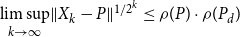
A major advantage of SDAs—regardless of a particular starting value—is that they provide quadratic convergence at relatively low computational cost per iteration. We establish sufficient conditions for quadratic convergence in the following theorem.
Theorem 3 (Convergence). Suppose
 $P$
and
$P$
and
 $P_d$
exist and satisfy Assumption
1
(and hence Corollary
1
). Then following statements are true.
$P_d$
exist and satisfy Assumption
1
(and hence Corollary
1
). Then following statements are true.
-
(1) If the sequences
$\{X_{k}\}_{k=0}^{\infty }$
,
$\{Y_{k}\}_{k=0}^{\infty }$
,
$\{E_{k}\}_{k=0}^{\infty }$
, and
$\{F_{k}\}_{k=0}^{\infty }$
are well defined, i.e., all the inverses exist during the doubling iteration process,
$X_k$
converges to
$P$
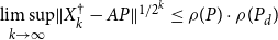
quadratically, and moreover,
$\limsup \limits _{k\rightarrow \infty } \lVert X_k - P\rVert ^{1/{2^k}} \leq \rho (P) \cdot \rho (P_d)$
. -
(2) If the sequences
$\{{X}^{\dagger }_{k}\}_{k=0}^{\infty }$
,
$\{{Y}^{\dagger }_{k}\}_{k=0}^{\infty }$
,
$\{{E}^{\dagger }_{k}\}_{k=0}^{\infty }$
, and
$\{{F}^{\dagger }_{k}\}_{k=0}^{\infty }$
are well defined, i.e., all the inverses exist during the doubling iteration process,
${X}^{\dagger }_k$
converges to
$AP$
quadratically, and moreover,
$\limsup \limits _{k\rightarrow \infty } \lVert {X}^{\dagger }_k - AP\rVert ^{1/{2^k}} \leq \rho (P) \cdot \rho (P_d)$
. -
(3) If the sequences
$\{L_{k}\}_{k=0}^{\infty }$
,
$\{H_{k}\}_{k=0}^{\infty }$
,
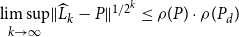
$\{\widehat {L}_{k}\}_{k=0}^{\infty }$
, and
$\{\widehat {H}_{k}\}_{k=0}^{\infty }$
are well defined, i.e., all the inverses during the Logarithmic Reduction exist,
$\widehat {L}_{k}$
converges to
$P$
quadratically, and moreover,
$\limsup \limits _{k\rightarrow \infty } \lVert \widehat {L}_{k} - P\rVert ^{1/{2^k}} \leq \rho (P) \cdot \rho (P_d)$
.


Proof. See the appendix.
Theorem 3 also applies to the cyclic reduction due to its equivalence to the SDA for SF2. Consequently, under Assumption 1, all algorithms presented above, from SDA for SF1 to logarithmic reduction, will converge quadratically to the unique (semi) stable solution
 $P$
.
$P$
.
4.3 Accuracy
To compare the different algorithms we need a measure of accuracy, that is, how far the solution produced by a particular method,
 $\hat {P}$
, is from the true solution,
$\hat {P}$
, is from the true solution,
 $P$
. As the latter is not known we will appeal to two measures, one from numerical stability analysis and another by comparing to arbitrary precision. For the numerical measure, we use the tighter forward error bound of Meyer-Gohde (Reference Meyer-Gohde2023)
$P$
. As the latter is not known we will appeal to two measures, one from numerical stability analysis and another by comparing to arbitrary precision. For the numerical measure, we use the tighter forward error bound of Meyer-Gohde (Reference Meyer-Gohde2023)
 \begin{align} \underbrace {\frac {\left \lVert P-\hat {P}\right \rVert _F}{\left \lVert P\right \rVert _F}}_{\text{Forward Error}}\le \underbrace {\frac {\left \lVert H_{\hat {P}}^{-1}\text{vec}\left (R_{\hat {P}}\right )\right \rVert _2}{\left \lVert \hat {P}\right \rVert _F}}_{\text{Forward Error Bound}} \end{align}
where the residual of the UQME is
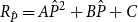 $R_{\hat {P}}=A\hat {P}^2+B\hat {P}+C$
and
$R_{\hat {P}}=A\hat {P}^2+B\hat {P}+C$
and
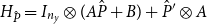 $H_{\hat {P}}=I_{n_y}\otimes (A\hat {P}+B)+\hat {P}'\otimes A$
, and the forward error relative to a high precision solution of the problem,
$H_{\hat {P}}=I_{n_y}\otimes (A\hat {P}+B)+\hat {P}'\otimes A$
, and the forward error relative to a high precision solution of the problem,
 $\hat {P}_{HP}$
,
$\hat {P}_{HP}$
,
 \begin{align} \underbrace {\frac {\left \lVert \hat {P}_{HP}-\hat {P}\right \rVert _F}{\left \lVert \hat {P}_{HP}\right \rVert _F}}_{\text{High Precision Forward Error}} \end{align}
The right-hand side of (35) can be rearranged so the numerator solves a Sylvester equation and we use the Advanpix Multiprecision Toolbox (Advanpix LLC., 2025) for
 $\hat {P}_{HP}$
.Footnote
12
We will see in the applications that the two measures provide essentially the same answer, which favors (35) that operates directly with the numerical solution,
$\hat {P}_{HP}$
.Footnote
12
We will see in the applications that the two measures provide essentially the same answer, which favors (35) that operates directly with the numerical solution,
 $\hat {P}$
. Nonetheless, having both measures should support belay skepticism in either particular measure.
$\hat {P}$
. Nonetheless, having both measures should support belay skepticism in either particular measure.
5. Applications
We run through two different sets of experiments to assess the SDAs—in the model of Smets and Wouters (Reference Smets and Wouters2007) and on the suite of models in the MMB. These two sets enable us to assess the different methods firstly in a specific, policy relevant model and then also in non-model specific manner, to give us insight on how robust our results are across models. We focus here on comparing our algorithms above with Dynare’s QZ-based method,Footnote 13 Dynare’s cyclic and logarithmic reduction methods,Footnote 14 the baseline Newton method from Meyer-Gohde and Saecker (Reference Meyer-Gohde and Saecker2024), and the baseline Bernoulli method from Meyer-Gohde (Reference Meyer-Gohde2025), who also run these experiments.Footnote 15 We assess the performance with respect to the accuracy, computational time, and convergence to the stable solvent. We examine the consequences of initializing both from zero matrix (an uninformed initialization of a stable solvent or the standard initialization for the reduction and structure preserving doubling algorithms) and Dynare’s QZ solution.
5.1 Smets and Wouters (2007) model
We start with Smets and Wouters’ (Reference Smets and Wouters2007) medium scale, estimated DSGE model that is a benchmark for policy analysis. They estimate and analyze a New Keynesian model with US data featuring the usual frictions, sticky prices and wages, inflation indexation, consumption habit formation as well as production frictions concerning investment, capital and fixed costs. For our purposes, the monetary policy rule is particularly important, as we will compare the accuracy of different solution methods when solving under alternate, but nearby parameterizations of the following Taylor rule
 \begin{gather} r_t=\rho r_{t-1} + (1-\rho ) \big(r_{\pi } \pi _t + r_{Y} (y_t - y_t^p) \big) + r_{\Delta y} \big(\big(y_t-y_t^p\big)-\big(y_{t-1}-y_{t-1}^p\big) \big) + \varepsilon ^r_t, \end{gather}
where
 $r_t$
is the interest rate,
$r_t$
is the interest rate,
 $\pi _t$
inflation, and
$\pi _t$
inflation, and
 $(y_t - y_t\,^p)$
the current output gap. The parameters
$(y_t - y_t\,^p)$
the current output gap. The parameters
 $r_{\pi }$
,
$r_{\pi }$
,
 $r_{Y}$
, and
$r_{Y}$
, and
 $r_{\Delta y}$
describing the sensitivity of the interest rate to each of these variables, and also the change in the output gap, and
$r_{\Delta y}$
describing the sensitivity of the interest rate to each of these variables, and also the change in the output gap, and
 $\rho$
measures interest rate smoothing.
$\rho$
measures interest rate smoothing.
The results for the posterior mode of Smets and Wouters (Reference Smets and Wouters2007) can be found in Table 1. Compared with the QZ algorithm, both the doubling algorithms, SF1 and SF2, along with the reduction algorithms already implemented in Dynare, perform very comparably. This is in contrast to the baseline Newton algorithm that fails to converge to the stable solvent (there is no guarantee that this algorithm will converge to a particular solvent though extensions of this baseline algorithm perform more favorably). The baseline Bernoulli algorithm gives a trade-off repeated throughout that analysis: generally more accurate, but often about an order of magnitude slower, than QZ. This is not the case with our doubling algorithms, they are as fast or faster than QZ and provide an order of magnitude more of accuracy. All four of the algorithms explored here, doubling and reduction, require about 10 iterations to converge and provide solutions that do not differ in an economic sense from the solution provided by QZ. Note that both of the measures of accuracy, the forward error bound in (35) and the error relative to a high precision solution (36), give similar results with the exception being the baseline Newton algorithm that solves the matrix quadratic, the forward error bound of (35) is small, but with a different solution than the rest of the algorithms—i.e., it converged to a solution containing unstable eigenvalues.
Smets and Wouters (Reference Smets and Wouters2007), posterior mode

Run Time for Dynare (QZ) in seconds, for all others, run time relative to Dynare. Max Abs. Diff. measures the largest abs. difference from the
 $P$
produced by Dynare.
$P$
produced by Dynare.
In Table 2 we examine the different methods as solution refinement techniques, by parameterizing the model of Smets and Wouters (Reference Smets and Wouters2007) to a numerical instability following Meyer-Gohde (Reference Meyer-Gohde2023), see the online appendix for this parameterization, and initializing the different methods at the Dynare QZ solution. Note that the reduction methods cannot work with an initial value for the solution, so we compare the solution provided by Dynare’s QZ with the doubling refinement versions of SF1 and SF2 as well as the Newton and the Bernoulli method. First, consistent with theorem 2 and, hence, the irrelevance of initial conditions for that algorithm, the SF2 algorithm does not appear to be comparable with the Newton or SF1 algorithm, converging to a solution that has a much less substantial improvement in accuracy. As above, the two different measures of accuracy we examine agree on the relative ordering of the different algorithms. The Newton algorithm provides substantially more accuracy than the Bernoulli algorithm but at a higher additional computational cost, echoing a trade-off mentioned above. The SF1 algorithm breaks through this barrier, providing roughly the same level of accuracy as the Newton algorithm at less computational costs. That the Newton method is so time consuming despite the relatively few number of iterations performed emphasizes the computational intensity of the Newton step that is not shared by the doubling algorithms—the former involves solving structured linear (Sylvester) equations whereas the latter solve standard systems of linear equations. The resulting implied variances of inflation,
 $\pi _t$
, differ on an economically relevant scale. The more accurate methods all agree that the QZ solution understates the variance of inflation.Footnote
16
$\pi _t$
, differ on an economically relevant scale. The more accurate methods all agree that the QZ solution understates the variance of inflation.Footnote
16
Smets and Wouters (Reference Smets and Wouters2007), numerically problematic parameterization

Run Time for Dynare in seconds, for all others, run time relative to Dynare. Variance
 $\pi _t$
gives the associated value for the population or theoretical variance of inflation.
$\pi _t$
gives the associated value for the population or theoretical variance of inflation.
We now take this refinement perspective and apply the different algorithms to solve iteratively for different parameterizations of the Taylor rule in the model of Smets and Wouters (Reference Smets and Wouters2007). We would like to establish whether solutions from previous, nearby parameterizations can be used to efficiently initialize the doubling methods similarly to the experiment above with the QZ solution as the initial guess. To that end, the experiment iterates through an evenly spaced
 $10\times 10$
grid for
$10\times 10$
grid for
 $r_\pi$
and
$r_\pi$
and
 $r_y$
, the responses to inflation and the output gap in the Taylor rule (37), holding all other parameters at their posterior mode values. We iterate through the grid taking the solution from the previous parameterization as the initialization for the next iteration, that is
$r_y$
, the responses to inflation and the output gap in the Taylor rule (37), holding all other parameters at their posterior mode values. We iterate through the grid taking the solution from the previous parameterization as the initialization for the next iteration, that is
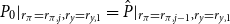 $P_{0}|_{r_\pi =r_{\pi ,j},r_y=r_{y,1}}=\hat {P}|_{r_\pi =r_{\pi ,j-1},r_y=r_{y,1}}$
initializing with
$P_{0}|_{r_\pi =r_{\pi ,j},r_y=r_{y,1}}=\hat {P}|_{r_\pi =r_{\pi ,j-1},r_y=r_{y,1}}$
initializing with
 $P_{0}|_{r_\pi =r_{\pi ,1},r_y=r_{y,1}}=\hat {P}^{QZ}|_{r_\pi =r_{\pi ,1},r_y=r_{y,1}}$
for the first row of the grid in the different values of
$P_{0}|_{r_\pi =r_{\pi ,1},r_y=r_{y,1}}=\hat {P}^{QZ}|_{r_\pi =r_{\pi ,1},r_y=r_{y,1}}$
for the first row of the grid in the different values of
 $r_\pi$
and then
$r_\pi$
and then
 $P_{0}|_{r_\pi =r_{\pi ,j},r_y=r_{y,j}}=\hat {P}|_{r_\pi =r_{\pi ,j},r_y=r_{y,j-1}}$
to fill out the grid in the values of
$P_{0}|_{r_\pi =r_{\pi ,j},r_y=r_{y,j}}=\hat {P}|_{r_\pi =r_{\pi ,j},r_y=r_{y,j-1}}$
to fill out the grid in the values of
 $r_y$
. Thus we initialize all algorithms at the QZ solution and, as we move to nearby parameterizations, we measure the time and accuracy of the different methods. We calculate the median over the whole grid and then repeat the experiment with the grid points closer together by varying the size of the interval in the grid—setting
$r_y$
. Thus we initialize all algorithms at the QZ solution and, as we move to nearby parameterizations, we measure the time and accuracy of the different methods. We calculate the median over the whole grid and then repeat the experiment with the grid points closer together by varying the size of the interval in the grid—setting
 $r_\pi \in [1.5,1.5 \times (1+10^{-x})]$
and
$r_\pi \in [1.5,1.5 \times (1+10^{-x})]$
and
 $r_Y \in [0.125,0.125 \times (1+10^{-x})]$
, where
$r_Y \in [0.125,0.125 \times (1+10^{-x})]$
, where
 $x \in [-1,8]$
. An increase in
$x \in [-1,8]$
. An increase in
 $x$
is a decrease in the spacing between the 100 grid points that thus increases the precision of the initialization.
$x$
is a decrease in the spacing between the 100 grid points that thus increases the precision of the initialization.
Forward errors and computation time per grid point for different parameterizations of the model by Smets and Wouters (Reference Smets and Wouters2007), log10 scale all axes.

Figure 1 summarizes the experiment graphically. Firstly, the left panel shows that the accuracy of the algorithms is independent of the grid spacing (and, hence, how close the parameter steps are from each other), this is expected and confirms the consistency of the algorithms and our measures of their accuracy.Footnote 17 The Bernoulli method is the exception and displays a significant drop in forward errors that coincides with the drop in computation time in the right figure—at a close enough parameterization, the Bernoulli algorithm starts with a guess from the previous parameterization that is accurate beyond the convergence threshold and the single iteration that is performed provides substantial (relative to more widely spaced grids) accuracy gains. In terms of their relative accuracies, the Newton is the most and the Bernoulli is generally (that is, except at the very closely spaced grids) the least accurate. All of the doubling and reduction algorithms are more accurate than QZ, with the cyclic reduction and SF2 algorithms roughly the same (as we would expect from Section 4.1) and close to Newton, followed by the log reduction, and finally SF1 doubling. As to be expected from Theorem 2, the SF2 doubling algorithm does not systematically profit in terms of reduced computation time as the parameter initializations improve (due to closer grid spacing) as the Newton and Bernoulli algorithms do. The SF1 doubling algorithm, in contrast, does profit with a downward trend in the computation time, although the Newton and Bernoulli algorithms clearly profit much more substantially with more significant downward trends.
5.2 MMB Suite Comparison
To guard against our comparison of methods from being specific to a particular model, we also adopt the model-robust approach inherit in the MMB. By abstracting from individual model characteristics we can gain insights into the algorithms that are robust to the particular features of a specific model. Besides drawing then general conclusions, we show an advantage for the SDAs with increasing model size. We implement version 3.3 of the MMB with the comparison repository Rep-MMB,Footnote 18 which contains over 160 different models, ranging from small scale to large-scale models and including estimated models of the US, EU, and multi-country economies. We test the algorithm on a subset of models appropriate for linear, rational expectations DSGE soution Footnote 19 —a histogram of the differing sizes can be found in Figure 2. With this large set of models, we feel confident in asserting that our assessment of the algorithms is robust to a representative sample of models relevant to policy settings.
Histogram over the number of state variables for the 142 MMB models.

We solve each model in the MMB first initializing with the zero matrix and then with the QZ solution provided by Dynare. To get a reliable measure of the computation times, we solve each model 100 times and take the average computation time of the middle three quintiles to minimize the effects of outliers.Footnote 20
MMB results

Run time and forward errors relative to Dynare, number of models that converge to the stable solution and number of iterations in absolute terms.
We begin with the initialization at the zero matrix and the top half of Table 3 summarizes the results. As noted in our previous studies, the Newton method is somewhat slower but more accurate than QZ when it converges to the stable solution—yet it does this in its baseline form only slightly more than half the time—and the baseline Bernoulli algorithm (almost) always converges to the unique stable solution—but does so more slowly than QZ at about the same level of accuracy. The cyclic reduction method is an intermediate case, converging to the stable solution for about 3/4 of the models, at generally comparable computation time, and somewhat higher accuracy than QZ. The logarithmic reduction is an improvement, converging for more models, and doing so at about the same speed and somewhat more accurately than the cyclic reduction. In terms of our doubling algorithms, they converge more frequently than even the logarithmic reduction (but still not for all and when, this failure is due to a breakdown of nonsingularity of the coefficient matrices in their recursions). As we will see in the next experiment, this can be overcome at least for the SF1 doubling algorithm by an appropriate (re)initialization of the algorithm.Footnote
21
The SF2 doubling algorithm on average outperforms QZ both in terms of speed and accuracy, although not for every model as the max or worst case shows (and again with the caveat that it does not successfully converge for 10 of the 142 models). The SF1 algorithm is not quite as fast at the median but has a far lower worst case computation time. This average performance of SF2 being faster than SF1 is consistent with the former inverting only one matrix,
 ${X}^{\dagger }_k - {Y}^{\dagger }_k$
—see Algorithm 2, whereas the latter needs to invert two,
${X}^{\dagger }_k - {Y}^{\dagger }_k$
—see Algorithm 2, whereas the latter needs to invert two,
 $I-{Y}_k {X}_k$
and
$I-{Y}_k {X}_k$
and
 $I-{X}_k{Y}_k$
—see Algorithm 1. Comparing the errors of the two doubling algorithms, SF2 has the lower worst case and mean forward error of the two and SF1 has the most accurate best case model and second best worst case model. Again, the information provided by the two error measures roughly coincides. In sum, the doubling algorithms (less so the reduction algorithms) perform favorably relative to QZ.
$I-{X}_k{Y}_k$
—see Algorithm 1. Comparing the errors of the two doubling algorithms, SF2 has the lower worst case and mean forward error of the two and SF1 has the most accurate best case model and second best worst case model. Again, the information provided by the two error measures roughly coincides. In sum, the doubling algorithms (less so the reduction algorithms) perform favorably relative to QZ.
Distribution of forward error bound for the MMB.

A graphical overview of the entire distribution of forward errors is plotted in Figure 3, the left relative to QZ and the right in absolute terms. The Newton algorithm is the most accurate with a clearly left shifted distribution relative to Dynare—with a mode improvement of about one order of magnitude—and the Bernoulli method the least with a clearly right shifted distribution relative to QZ. All of the methods here, reduction and doubling, lie in between but with modes and medians all to the left of QZ. While they are all very comparable, the SF2 algorithm has almost its entire mass to the left of Dynare and the cyclic reduction algorithm is right skewed with a substantial mass to the right of Dynare. The absolute values show that almost all of the models have errors less than 1e-10 and the accuracy of the Newton method is also clear with a substantial mass of forward error bounds inside machine precision and all mass essentially below e-12. The distributions of forward errors relative to the high precision solution (36) give virtually the same picture, as we show in Figure 4c. In any case, it appears that the models in the MMB were solved with acceptable accuracy and the SF2 doubling or logarithmic reduction is to be preferred among the algorithms here.
Forward errors and computation time, log10 scales, for the MMB.

Figure 4 provides a model-by-model comparison of the different algorithms’ performance relative to QZ with each dot being the result of a model. All four panels express computation times and forward errors relative to Dynare on a log scale—hence a negative value in a dimension means the algorithm is more accurate or computationally efficient than QZ. In the top left panel, all of the methods are plotted using the forward error bound. First, recognize that the Bernoulli method is sometimes more and sometimes less accurate than QZ but usually slower (higher computation time), whereas the baseline Newton method is generally more accurate but usually slightly slower than QZ. The doubling and reduction algorithms require similar computation times as QZ (almost always within one half an order of magnitude slower/faster) but are generally more accurate. The doubling algorithms are more accurate than the reduction algorithms (notice the outlier along the x axis of the reduction algorithms with more than three orders of magnitude higher forward errors than QZ) and the SF2 doubling algorithm is the most accurate of the doubling algorithms as can be seen by comparing the lower two panels—visually, this algorithm is on average slightly faster than QZ and provides an order of magnitude more accuracy. The upper right panel plots the forward error relative to a high precision solution to the numerical forward error bound—as all points, hence the solutions from all algorithms for all models, lie along the 45 degree line, we conclude these two measures provide the same information. This provides strong evidence in favor of Meyer-Gohde (Reference Meyer-Gohde2023) practical forward error bound (35) that calculates this bound without having to calculate an additional, computationally expensive higher precision solution, but rather operates through the numerical stability analysis of the solution provided by the method in question only.
Forward errors, computation time, and state variables for MMB.

Figure 5 continues the model-by-model comparison of the different algorithms’ performance relative to QZ, but now with a focus on the effect of model size, measured by the number of state or backward-looking variables. The top left panel gives the accuracy of the different methods for the different models plotted against the dimension of the endogenous state. There is not a visually compelling correlation—although for very large models, the reduction and doubling algorithms like the Newton algorithm appear to perform better than QZ. For computational times the story is different: the right panel plots the computational time against the number of state variables and a clear downward trend or negative correlation in particular for the doubling algorithms is obvious. In sum, for the largest models in the MMB, our doubling algorithms provide about two orders of magnitude more accuracy at about one tenth the computation time.
To assess the potential for improving on solutions, we repeat the exercise, but now initialize with the solution provided by QZ, see the bottom half of Table 3 for the results. The cyclic and logarithmic reductions are no longer included as they cannot operate with an arbitrary initialization. The baseline Newton method significantly improves the number of models it converges for. Note especially that, in contrast to the top half of the table when initialized at the zero matrix, now the SF1 doubling algorithm alongside the baseline Bernoulli method converges successfully to the unique stable solution in all models. Consistent with theorem 2, the SF2 doubling algorithm, however, does not and continues to converge or not for all but one of the same models as under the initialization with the zero matrix.
Both the Bernoulli and Newton methods run just a few iterations, and the later generally achieves a greater increase in accuracy albeit at a higher additional computation cost due to the computational intensity of the Newton step. The SF1 and SF2 doubling algorithms run through multiple iterations, ending up being faster and slightly more accurate than the Newton method at the median. Far more impressive here are the max or worst-case outcomes, with SF1 doubling at worst adding on an additional 7.5 times QZ computation cost and 4.9 times the forward error. The worst case Newton computation costs are an additional 840 times and Bernoulli 50+ thousand times the QZ initial time and the SF2 doubling algorithm has at worst a forward error bound about 300 times and Newton 1e9 times that of QZ. The results also highlight the effects of finite precision: numerical calculations generally introduce nonzero numerical errors, e.g. rounding errors, and if QZ’s solution is already accurate up to machine precision, additional calculations with any algorithm are unlikely to increase and more likely to decrease accuracy. We conclude that the SF1 doubling algorithm ought to be preferred as a solution refinement method, usually providing significant accuracy gains at low additional computation costs that is robust even in the worst case relative to alternatives.
Figure 6, like Figure 3 but now initialized at the QZ solution, provides an overview of the entire distribution of forward errors, the left relative to those from Dynare’s QZ method and the middle in absolute terms. We display the results from the forward error bound and, again, the forward error relative to a high precision solution gives the same picture, as confirmed by the figure on the right. It is apparent that the baseline Bernoulli algorithm provides only a marginal improvement on the QZ solution. While this should be tempered with the observation that only two Bernoulli iterations were performed at the median, the Newton algorithm also only runs a few iterations. The doubling algorithms perform favorably, with both displaying left shifted distributions of error bounds relative to QZ. Taken together with the results from Table 3, the SF1 doubling algorithm can be considered an ideal solution refinement algorithm across a wide variety of models.
Distribution of FE bound for the MMB, initialized at dynare (QZ).

6. Conclusion
We have introduced and developed doubling algorithms for solving linear DSGE models as alternatives to QZ methods, connecting them to the related reduction algorithms implemented, albeit silently, in Dynare. The doubling algorithms possess quadratic convergence rates, combining the advantages of Newton-based methods with the stable solution properties of Bernoulli methods. This paper demonstrates their practical value through extensive testing, particularly in comparison to the literature-standard QZ algorithm and in their ability to refine existing solutions for improved accuracy.
Our experiments, including applications to the Smets and Wouters (Reference Smets and Wouters2007) model and the suite of models in the MMB, reveal that both doubling algorithms outperform QZ in accuracy and computational efficiency across a wide range of models. For the largest model in the MMB with thousands of state variables, doubling algorithms achieve solutions roughly an order of magnitude faster than QZ, highlighting their potential in computationally intensive settings, such as heterogeneous agent models like HANK. These findings underscore the relevance of doubling algorithms for large-scale macroeconomic modeling, particularly when speed and precision are critical.
While results across the MMB are generally favorable, outliers remain in terms of accuracy, computational time, and convergence. To address such variability, we extended the doubling algorithms to accept user-defined initializations, providing convincing evidence that the SF1 doubling algorithm in particular can reliably deliver low-cost, high-accuracy refinements of existing solutions. In scenarios where improving the accuracy of an initial solution is paramount, the SF1 doubling algorithm is the algorithm of choice, combining robustness, speed, and precision. The methods provide promising alternatives, particularly when working with large-scale or computationally intensive DSGE models.
Supplementary material
The supplementary material for this article can be found at https://doi.org/10.1017/S1365100525100813.
Acknowledgements
We are grateful to participants of the 30th International Conference on Computing in Economics and Finance (2024 CEF) and the Annual Conference of the International Association for Applied Econometrics (IAAE 2024). The code to replicate the analysis can be found at https://github.com/AlexMeyer-Gohde/Linear-DSGE-with-Doubling. This research was supported by the DFG through grant nr. 465469938 “Numerical diagnostics and improvements for the solution of linear dynamic macroeconomic models” and grant nr. 465135565 “Models of Imperfect Rationality and Redistribution in the Context of Retirement.”
Appendix A. Proof of Theorem 2
We can show the statement by induction. For
 $k=0$
we have
$k=0$
we have
 \begin{align*} \widehat {X}^{\dagger }_{0}&=-AP_0 ={X}^{\dagger }_{0}-AP_0,&\widehat {Y}^{\dagger }_{0}&=-AP_0-B ={Y}^{\dagger }_{0}-AP_0,& \widehat {E\,}^{\dagger }_{0}&=-C ={E}^{\dagger }_{0},& \widehat {F}^{\dagger }_{0}&=-A ={F}^{\dagger }_{0}. \end{align*}
Further, assuming that the claim holds for an arbitrary
 $k\geq 0$
we have
$k\geq 0$
we have
 \begin{align*} \left (\widehat {X}^{\dagger }_k - \widehat {Y}^{\dagger }_k\right ) &=\left ({X}^{\dagger }_k - AP_0 - {Y}^{\dagger }_k + AP_0\right )= \left ({X}^{\dagger }_k - {Y}^{\dagger }_k\right ), \end{align*}
and therefore
 \begin{gather*} \widehat {E\,}^{\dagger }_{k+1} =\widehat {E\,}^{\dagger }_k \left (\widehat {X}^{\dagger }_k - \widehat {Y}^{\dagger }_k\right )^{-1} \widehat {E\,}^{\dagger }_k={E}^{\dagger }_k \left ({X}^{\dagger }_k - {Y}^{\dagger }_k\right )^{-1} {E}^{\dagger }_k = {E}^{\dagger }_{k+1}\\ \widehat {F}^{\dagger }_{k+1} =\widehat {F}^{\dagger }_k \left (\widehat {X}^{\dagger }_k - \widehat {Y}^{\dagger }_k\right )^{-1} \widehat {F}^{\dagger }_k={F}^{\dagger }_k \left ({X}^{\dagger }_k - {Y}^{\dagger }_k\right )^{-1} {F}^{\dagger }_k = {F}^{\dagger }_{k+1} \\ \widehat {X}^{\dagger }_{k+1} =\widehat {X}^{\dagger }_k - \widehat {F}^{\dagger }_k \left (\widehat {X}^{\dagger }_k - \widehat {Y}^{\dagger }_k\right )^{-1} \widehat {E\,}^{\dagger }_k={X}^{\dagger }_k - AP_0 -{F}^{\dagger }_k \left ({X}^{\dagger }_k - {Y}^{\dagger }_k\right )^{-1} {E}^{\dagger }_k ={X}^{\dagger }_{k+1} - AP_0 \\ \widehat {Y}^{\dagger }_{k+1} =\widehat {Y}^{\dagger }_k + \widehat {E\,}^{\dagger }_k \left (\widehat {X}^{\dagger }_k - \widehat {Y}^{\dagger }_k\right )^{-1} \widehat {F}^{\dagger }_k={Y}^{\dagger }_k - AP_0 + {E}^{\dagger }_k \left ({X}^{\dagger }_k - {Y}^{\dagger }_k\right )^{-1} {F}^{\dagger }_k = {Y}^{\dagger }_{k+1} - AP_0.\\ \end{gather*}
Appendix B. Proof of Theorem 3
For the proofs of parts (1) and (2) see Theorems 3.18 and 3.19 by Huang et al. (Reference Huang, Li and Lin2018, pp. 35, 37). To prove (3) first note that Assumption 1 (and hence Corollary 1) implies
 $\rho (P) \leq 1 \wedge \rho (P_d) \lt 1$
.
$\rho (P) \leq 1 \wedge \rho (P_d) \lt 1$
.
We will show that in this case
 $H_k$
converges quadratically to zero. To see this, note that using (33) of UQME (5) and it’s dual UQME
$H_k$
converges quadratically to zero. To see this, note that using (33) of UQME (5) and it’s dual UQME
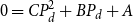 $0=C P_d^2 + B P_d +A$
, respectively, we receive
$0=C P_d^2 + B P_d +A$
, respectively, we receive
 \begin{align} L_{k} &= \mathscr{M}_{k} - H_{k} \mathscr{M}_{k}^{\,2},& H_{k} &= \mathscr{N}_{k} - L_{k} \mathscr{N}_{k}^{\,\,2} \end{align}
where
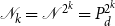 $\mathscr{N}_{k}=\mathscr{N\,\,}^{2^{k}}=P_{d}^{2^{k}}$
. Using (A1) to substitute
$\mathscr{N}_{k}=\mathscr{N\,\,}^{2^{k}}=P_{d}^{2^{k}}$
. Using (A1) to substitute
 $L_{k}$
in the right equation of (A1) yields
$L_{k}$
in the right equation of (A1) yields
 \begin{align} H_{k} &= \mathscr{N}_{k} - \mathscr{M}_{k}\mathscr{N}_{k}^{\,\,2} + H_{k} \mathscr{M}_{k}^{\,2} \mathscr{N}_{k}^{\,\,2} \end{align}
Thus, for any sub-multiplicative matrix norm
 $\lVert \,.\,\rVert$
we obtain
$\lVert \,.\,\rVert$
we obtain
 $\lVert H_{k}\rVert \leq \lVert \mathscr{N}_{k}\rVert + \lVert \mathscr{M}_{k}\rVert \lVert \mathscr{N}_{k}\rVert ^{2} + \lVert H_{k}\rVert \lVert \mathscr{M}_{k}\rVert ^{2} \lVert \mathscr{N}_{k}\rVert ^{2}$
. Since
$\lVert H_{k}\rVert \leq \lVert \mathscr{N}_{k}\rVert + \lVert \mathscr{M}_{k}\rVert \lVert \mathscr{N}_{k}\rVert ^{2} + \lVert H_{k}\rVert \lVert \mathscr{M}_{k}\rVert ^{2} \lVert \mathscr{N}_{k}\rVert ^{2}$
. Since
 $\rho (P) \cdot \rho (P_d)=\rho (\mathscr{M}) \cdot \rho (\mathscr{N}\kern1pt\,) \lt 1$
defining
$\rho (P) \cdot \rho (P_d)=\rho (\mathscr{M}) \cdot \rho (\mathscr{N}\kern1pt\,) \lt 1$
defining
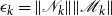 $\epsilon _k=\lVert \mathscr{N}_{k}\rVert \lVert \mathscr{M}_{k}\rVert$
we know that
$\epsilon _k=\lVert \mathscr{N}_{k}\rVert \lVert \mathscr{M}_{k}\rVert$
we know that
 $\lim \limits _{k\rightarrow \infty } \epsilon _k = 0$
. Hence, there is some sufficiently large
$\lim \limits _{k\rightarrow \infty } \epsilon _k = 0$
. Hence, there is some sufficiently large
 $k$
so that
$k$
so that
 $\epsilon _k\lt 1$
and consequently
$\epsilon _k\lt 1$
and consequently
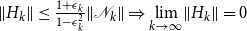 $\lVert H_{k}\rVert \leq \frac {1 + \epsilon _k}{1-\epsilon _k^2} \lVert \mathscr{N}_{k}\rVert \Rightarrow \lim \limits _{k\rightarrow \infty } \lVert H_{k}\rVert = 0$
. From the Gelfand’s formula / the spectral radius theorem we also know
$\lVert H_{k}\rVert \leq \frac {1 + \epsilon _k}{1-\epsilon _k^2} \lVert \mathscr{N}_{k}\rVert \Rightarrow \lim \limits _{k\rightarrow \infty } \lVert H_{k}\rVert = 0$
. From the Gelfand’s formula / the spectral radius theorem we also know
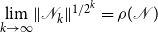 $\lim \limits _{k\rightarrow \infty } \lVert \mathscr{N}_{k}\rVert ^{1/{2^k}} = \rho (\mathscr{N}\kern1pt\,)$
so that
$\lim \limits _{k\rightarrow \infty } \lVert \mathscr{N}_{k}\rVert ^{1/{2^k}} = \rho (\mathscr{N}\kern1pt\,)$
so that
 \begin{equation*}\lVert H_{k}\rVert ^{1/{2^k}} \leq \left (\frac {1 + \epsilon _k}{1-\epsilon _k^2}\right )^{1/{2^k}} \lVert \mathscr{N}_{k}\rVert ^{1/{2^k}} \Rightarrow \lim \limits _{k\rightarrow \infty } \lVert H_{k}\rVert ^{1/{2^k}} = \rho (\mathscr{N}\kern1pt\,) \leq \rho (P_d).\end{equation*}
Since
 $\rho (P_d)\lt 1$
we know that
$\rho (P_d)\lt 1$
we know that
 $H_{k}$
converges quadratically to zero. Hence, we also know that there must be some sufficiently large
$H_{k}$
converges quadratically to zero. Hence, we also know that there must be some sufficiently large
 $k$
such that
$k$
such that
 $\lVert \widehat {H}_{k-1} \rVert = \lVert H_{0} \cdot \ldots \cdot H_{k-1} \rVert \lt 1$
and consequently
$\lVert \widehat {H}_{k-1} \rVert = \lVert H_{0} \cdot \ldots \cdot H_{k-1} \rVert \lt 1$
and consequently
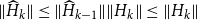 $\lVert \widehat {H}_{k}\rVert \leq \lVert \widehat {H}_{k-1}\rVert \lVert H_{k}\rVert \leq \lVert H_{k}\rVert$
. This means that
$\lVert \widehat {H}_{k}\rVert \leq \lVert \widehat {H}_{k-1}\rVert \lVert H_{k}\rVert \leq \lVert H_{k}\rVert$
. This means that
 $\widehat {H}_{k}$
also converges quadratically to zero, i.e.,
$\widehat {H}_{k}$
also converges quadratically to zero, i.e.,
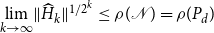 $\lim \limits _{k\rightarrow \infty } \lVert \widehat {H}_{k}\rVert ^{1/{2^k}} \leq \rho (\mathscr{N}\kern1pt\,) = \rho (P_d)$
. Now rewrite the right equation of (33) to
$\lim \limits _{k\rightarrow \infty } \lVert \widehat {H}_{k}\rVert ^{1/{2^k}} \leq \rho (\mathscr{N}\kern1pt\,) = \rho (P_d)$
. Now rewrite the right equation of (33) to
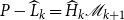 $P - \widehat {L}_{k} = \widehat {H}_{k} \mathscr{M}_{k+1}$
to yield
$P - \widehat {L}_{k} = \widehat {H}_{k} \mathscr{M}_{k+1}$
to yield
 $ \lVert P - \widehat {L}_{k}\rVert \leq \lVert \widehat {H}_{k} \rVert \lVert \mathscr{M}_{k+1}\rVert$
. The statement then follows from the Gelfand’s formula / the spectral radius theorem as
$ \lVert P - \widehat {L}_{k}\rVert \leq \lVert \widehat {H}_{k} \rVert \lVert \mathscr{M}_{k+1}\rVert$
. The statement then follows from the Gelfand’s formula / the spectral radius theorem as
 \begin{align} \lVert P - \widehat {L}_{k}\rVert ^{1/{2^k}} &\leq \lVert \widehat {H}_{k} \rVert ^{1/{2^k}} \lVert \mathscr{M}_{k+1}\rVert ^{1/{2^k}} \Rightarrow \lim \limits _{k\rightarrow \infty } \lVert P - \widehat {L}_{k}\rVert ^{1/{2^k}} \leq \rho (P)\rho (P_d). \end{align}
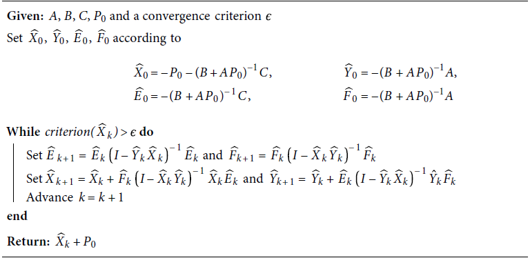
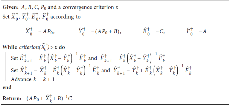
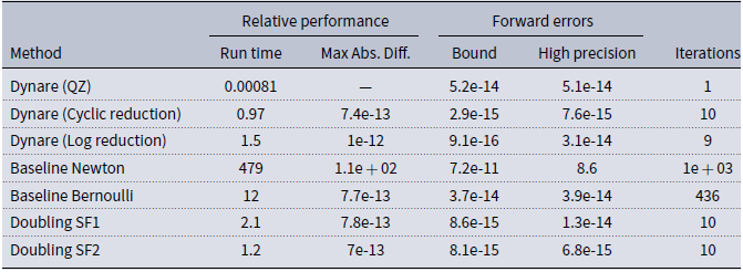


 Open access