Introduction

In the study of glaciofluvial sediment transport, most works have dealt with relationships between discharge and suspended-sediment transport (Reference Østrem, Jopling and McDonaldOstrem, 1975; Reference CollinsCollins, 1979; Reference GurnellGurnell, 1982). Less consideration has been given to grain-size distributions of sediments transported or settled in glacial meltwater streams (Reference Rainwater and GuyRainwater and Guy, 1961; Ziegler, 1974; Reference Bogen, Enell and GahnströmBogen, 1979,1980; Reference Fenn and GomezFenn and Gomez, 1989), whereas several investigations of this subject have been carried out in non-glaciated areas (Reference Folk and WardFolk and Ward, 1957; Reference BagnoldBagnold, 1968; Reference VisherVisher, 1969; Reference SenguptaSengupta, 1975; Reference MiddletonMiddleton, 1976; Reference Walling and MooreheadWalling and Moorehead, 1987).

However, Ziegler (1974) emphasized the necessity of analysing the composition of suspended sediment, as water from proglacial streams is used in hydro-electric power stations. As argued by Reference Walling and MooreheadWalling and Moorehead (1987), the grain-size of suspended sediments may also exert an important control on the trap efficiency of reservoirs. Additionally, the study of grain-size distributions can provide important information on the interactions between discharge and glacial hydrology, on the one hand, and factors such as composition of till at the glacier bed or stream-bed material, on the other.

This study aims to consider temporal variations in grain-size distribution of suspended sediment in a glacial meltwater stream and compare the variations with discharge and sediment concentration.

Study Area

Field work was undertaken in the summer of 1985 at Austre Okstindbreen, the largest glacier in Okstindan, northern Norway (Fig. 1). The glacier covers an area of 14 km² between about 1700 and 730 m, and the catchment of the limnigraph station, where discharge was measured, has an area of 22.5 km². However, water contributions from areas outside the drainage basin of Austre Okstindbreen are only of minor and decreasing influence, as snow melt declines and ice melt increases during the summer. Though rainfall is very common, its contribution to the drainage is of minor importance. Generally, two meltwater streams, a southern and a northern one, drain the glacier (Reference Theakstone and KnudsenTheakstone and Knudsen, 1981). At the beginning of the field season, the southern stream was the major one, but it contained only negligible amounts of sediment in transport. However, after a mid-July storm, followed by an extraordinarily high discharge, no flow was registered in this outlet. Because of the very difficult conditions in the northern stream, where samples were taken, it was not possible to carry out discharge measurements there, but the water-level fluctuations appeared to be perfectly in phase with the fluctuations at the site where the discharge was measured.

Fig. 1.

The location of Okstindan and Austre Okstindbreen with glacier margins of 1962 and 1985.

Fig. 2.

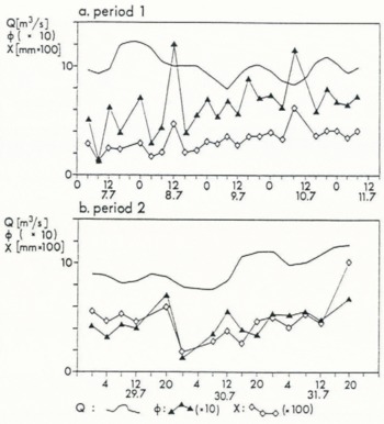
The course of discharge (Q), mean grain-size (x), and percentage of fine sediment (ø) during periods 1(a) and 2(b).

Petrographically, the area is very monotonous (Reference HoelHoel, 1910). It consists mainly of garnetiferous mica-schists. However, at several locations, granitic dykes occur, and in places dolomite is present. In front of the glacier, the area is dominated by morainic material consisting of rock fragments and finer sediments.

Methods

Using a Manning S-4050A automatic sampler, meltwater was collected at intervals of 2 h. Every second sample from two distinct periods in the field season (Fig. 2) was used for grain-size analysis. The water intake, a tube of 9.5 mm internal diameter, was fixed in the stream well off the bed about 30 m from the glacier portal and about 2 m from the channel bank. The sampler was adjusted to an intake velocity of 1 m s⁻¹, and stream-flow velocity near the intake was measured to between 0.3 and 0.9 ms⁻¹.

Meltwater samples, which usually contained between 170 and 240 ml, were filtered within 48 h after sampling through individually pre-weighed Schleicher and Schüll cellulose membrane filter papers (0.45 μm pore diameter), air-dried and packed into aluminium foil and numbered plastic bags.

In the laboratory, the filter papers were dried for 16 h at 110°C. Before weighing, the few grains coarser than

1 mm were removed from the samples, because their large individual weights would influence the statistical analyses of the samples (all of which are small) in a random manner. However, it was only necessary to remove grains from a few samples.

In order to prepare the samples for analysis, filter papers were individually oven-destructed (1 h at 200°C), and the sediments were treated with 0.002 mol sodium pyrophosphate and ultra-sound to prevent flocculating grains. Grain-size fractions coarser than 0.038 mm were dried and sieved for 20 min using the factor 2 scale, while fractions finer than that size were analysed by means of sedimentation.

The statistical analyses of the grain-size data were based on the hyperbolic distribution. Ina log-log plot, the probability function of a hyperbolic distribution appears as a hyperbola, whereas a log-log plot of the probability function of a normal distribution appears as a parabola. Strictly speaking, the normal distribution represents only one single shape of curve, while the hyperbolic distribution, with the same variance, includes an association of curve shapes. Several investigations have shown that the distributions of wind- and water-transported and -deposited sediments are better described as hyperbolic than log-normal (Reference Bagnold and BarndorfT–NielsenBagnold and Barndorff-Nielsen, 1980). The estimation programme SAHARA (Christiansen and Hartmann, 1988) was used to approximate the hyperbolic distribution to the data (Fig. 3). Mathematical descriptions of the hyperbolic distribution are found in, for example, Reference NielsenBarndorff-Nielsen (1977) and Reference NielsenBarndorff-Nielsen and others (1982).

Fig. 3.

a. Shows the hyperbolic curve fitted for a sample of grain-size data from period 1. The figure at the top indicates the number of the sample, b. Shows the positions of 23 distributions from the two periods in the shape triangle of the hyperbolic distribution (χ = skewness; ξ = peakedness). All other distributions of suspended sediments from this study are placed on the line: ξ = 1.0 (χ < –0.4). In addition, three distributions of settled samples from a lake in front of the glacier, and eight distributions from the work of Reference Fenn and GomezFenn and Gomez (1989) are shown. The normal distribution (N), the positive and negative hyperbolic (H and —H), and exponential (E and -E) distributions, and the Laplace distribution are limits of the hyperbolic distribution (after Reference Nielsen and ChristiansenBarndorff-Melsen and Christiansen, 1988).

Table 1.

Correlation coefficients between selected parameters and number of samples. The α values show the results of two-tailed analysis of the correlation coefficients. If α exceeds 0.05, the coefficient is not significantly different from zero. The subscript in the equation which gives the best correlation coefficient: 1: Y = a + bX; 2: Y = aX^b; 3: Y = e^{(a + bX)}

Results

Results of the analyses of grain-size distributions are shown in Tables 1 and 2 and in Figures 2 and 3. It is emphasized that no samples were normally distributed. This is clearly shown in Figure 3b. In order to compare with the distributions of settled sediments in the same environment, three samples collected during the 1985 field season are plotted in the figure, and they appear to be clearly different from the others. Furthermore, eight samples from the work of Reference Fenn and GomezFenn and Gomez (1989) on the same subject are plotted in the figure in order to compare with suspended sediments from another location. Though their shapes are different from the others, as seen in the figure, they are far from being normally distributed.

Table 1 shows correlations from both periods between discharge and selected sediment-describing and distribution-describing parameters.

Large variations in correlation coefficients occur, indicating differences in influence of different parameters, both within the individual periods and between them.

There is high correlation between discharge, Q and sediment concentration, c, in period 2, but practically none in period 1, with correlation coefficients calculated for the period as a whole. However, if the development of Q and c is split up into single days or events, good correlations are found in both periods.

The correlation between sediment concentration and the coarse fractions, expressed by γ (cf. Fig. 3a), is much higher in period 2 than in period 1. The same holds for the comparison of the prevailing grain-size, v, and sorting, κ, while the opposite is the case between mean grain-size, x, and skewness, χ.

Almost no correlation is found between discharge and the concentration of sand (<1 mm) in period 1 while there is high correlation between those parameters in period 2.

Table 2.

Comparison of mean values (M) and standard deviations (s) of periods 1 and 2. Explanation of subscripts: 1. Does not reject the hypotheses that sl = s2; 2. Reject this hypothesis; 3. Does not reject the hypothesis that Ml = M2; 4. Reject this hypothesis. The symbols F and t indicate the F- and t-tests, respectively

The same holds for the comparison of the prevailing grain-size and the concentration of silt (and clay, which is included here).

In period 1, mean grain-size seems to describe the distributions better than the prevailing grain-size does. In period 2, however, neither of them can be said to be better than the other.

Table 2 compares parameters from period 1 with parameters from period 2. In most cases, standard deviations and mean values are significantly different between the two periods.

It is worth noting that, though the mean sediment concentration is much lower in period 2, the percentage of coarse grains is larger. The removal of grains, as mentioned before, was only necessary from samples in this period.

Figure 2 visualizes relations between discharge- and distribution-describing parameters. It is seen that the variations of mean grain-size and percentage of fine material, Φ (defined as the fraction which is finer than the prevailing grain-size), coincide, but the correlation with discharge is low. The slow increase of Φ and x through period 1 and through the greater part of period 2 shows that the percentage of fine material decreases.

Discussion

The results presented in Table 2 indicate that conditions other than hydraulic ones are responsible for the grain-size distribution of the suspended sediment. This is in agreement with the results of Reference Bogen, Enell and GahnströmBogen (1979), who studied grain-size distributions of suspended sediment in several Norwegian proglacial and non-glacial streams. Bogen drew his conclusion from the unfilfilled requirement that the sediments should be normally distributed. However, it is unlikely that hydraulics result in normally distributed sediments. Reference Kennedy, Ehrlich and KanaKennedy and others (1981) showed that suspended sediments below breaking waves were distributed non-log-normally. Reference Bagnold and BarndorfT–NielsenBagnold and Barndorff-Nielsen (1980) and Reference Christiansen, Blaesild and DalsgaardChristiansen and others (1984) showed that sediments transported by water are better described by using hyperbolic distributions. Additionally, the latter authors showed that the segmented curves which often appear when plotting grain-size data on probability paper have the same course as hyperbolic distributions plotted on the same paper. Applying this to the curves given by Bogen, it can be shown that his samples can also be described as hyperbolic or by the (skew) Laplace distribution.

Reference Rainwater and GuyRainwater and Guy (1961) found that variations in grain-size distribution coincided well with discharge in the meltwater stream draining Chamberlain Glacier, Alaska. The difference between their findings and those of the present study may be due to the fact that Rainwater and Guy sampled about 250 m from the glacier (30 m in this study). Using data from their paper, it can be shown that none of the samples was normally distributed, though some of them also were neither hyperbolic.

Reference Fenn and GomezFenn and Gomez (1989) made use of cross-correlation analysis in order to find connections between discharge and distribution parameters (median grain-size and sorting according to Reference TraskTrask (1930)). They found that the values were broadly in phase with discharge, but correlation coefficients never exceeded 0.30, a result which is in general agreement with the results of the present study. As mentioned before and seen in Figure 3b, the sediment studied by Fenn and Gomez also turned out to have a hyperbolic distribution (grain-size data kindly supplied by C.R. Fenn).

The importance of using the hyperbolic distribution for the description of sediment samples is illustrated by the fact that a fit of the normal distribution to cumulative grain-size data often results in a segmented curve. This curve has mostly been interpreted as belonging to two or three separate normal distributions (cf. Reference VisherVisher, 1969; Reference MiddletonMiddleton, 1976), which were said to have originated by different transport mechanisms. However, even samples which are taken from suspension, reflecting a single transport type, may appear as segmented curves if fitted by normal distributions. For this reason, the uncritical use of normal distributions may well lead to errors in interpretation of sediment sources. Additionally, the ability of fitting a single distribution, whether it is hyperbolic, normal, or of any other kind, to sediment samples may help to eliminate such errors.

The non-hydraulic conditions which influence the grain-size distributions of the suspended sediment must be searched for either subglacially or at the stream bed (which of course can also be subglacial).

Reference CollinsCollins (1979) studied variations in suspended-sediment concentration in the proglacial river Gornera, Switzerland, and the connection with subglacial events. He suggested that slumping from unstable moraines may cause sudden increases in concentration. A similar process can often be observed on river banks, where erosion and removal of fine sediments cause the whole bank or part of it to slump into the water. The decrease in relative content of fine sediment through the first and the last part of the second period, as indicated in Figure 2, may well give reason to invoke such processes. As sediments in moraines tend to be very poorly sorted, the reason for the erratic changes in grain-size distribution could be found in Collins’ suggestions.

Reference BogenBogen (1980) found that temporary deposition and erosion of sediments at the channel bed during falling and rising stages of water caused short time variations in grain-size distributions. He concluded that this, together with flow competence, was the determinant condition.

It is possible to believe that mixing of the two factors suggested by Collins and Bogen will determine the sediment composition. However, referring to the results of Rainwater and Guy, hydraulics will probably influence the grain-size distributions more with increasing distance from the glacier, as the importance of subglacial sediment sources declines. In addition, it should be expected that, because of the chosen sampling site, the hydraulic influence in the present study exists but is disguised by the factors mentioned above.

Several workers have used parameters from grain-size distributions for environmental distinctions (e.g. Reference FriedmanFriedman, 1961; Reference KoldijkKoldijk, 1968). Reference Nielsen and ChristiansenBarndorff-Nielsen and Christiansen (1988) used the hyperbolic shape triangle for distinguishing between erosion and deposition of sand. Figure 3b indicates that the hyperbolic shape triangle may be useful for such identifications. First, a clear distinction can be made between the distributions of transported and settled sediment, respectively, which is clear, as a certain kind of sorting takes place during the settling process, causing a change in curve shape. The settled sediments shown in Figure 3b are much better sorted than the suspended sediments. Secondly, through a comparison of distribution shapes from two separate locations, as seen in this figure, it seems that the initial conditions (which could be mineralogical or grain-size compositions, respectively, and accessibility for weathering, erosion, and transport) probably play the most important role in the grain-size distribution of the suspended sediment. The reason for this suggestion is that one should expect hydraulics to influence grain-size independently of location.

The comparative, statistical tests of parameters from periods 1 and 2 in Table 2 indicate the existence of two distinct sediment populations. This implies that emptying of discrete sediment reservoirs is taking place, which is possible in various ways. Reference CollinsCollins (1979) mentioned that the drainage of an ice-dammed lake at Gornergletscher, Switzerland, caused an evacuation of sediment from the glacier bed. Furthermore, the development of the glacial drainage system during the summer causes the opening of englacial and subglacial conduits, resulting in drainage of reservoirs and the release of sediments. Additionally, glacier movement may deform conduits, resulting in opening or closing of drainage systems. Reference Theakstone and KnudsenTheakstone and Knudsen (1981) carried out dye-tracer tests at Austre Okstindbreen. They found that the drainage pattern in the glacier was built up of several minor conduits which joined the main stream (or streams) before leaving the glacier. Over several years, Reference Knudsen and TheakstoneKnudsen and Theakstone (1988) studied the drainage of an ice-dammed lake at Austre Okstindbreen. In 1985, the drainage of the lake occurred just before the beginning of the period of observation for the present study, and it is believed that large amounts of sediment were removed from the glacier bed during the flood. As the extraordinarily high discharge in the mid-season of 1985 cannot be explained by intensive precipitation or increased melting, it must be inferred that it was caused by the release of an internal reservoir, which further blocked the conduits leading to the southern outlet and thereby changed the main drainage system of Austre Okstindbreen.

The gradual increase of the parameters Φ and x during period 1 (Fig. 2a) indicates the emptying of a sediment reservoir, meaning that the finest sediments are removed first. After the first third of period 2, the increase of Φ and x (Fig. 2b) shows that a new emptying of a sediment reservoir works through.

Conclusions

In the light of the results and discussion of the present study, the following conclusions can be drawn:

1. 1. Grain-size distributions of suspended sediments in glacial melt-water streams can be described as hyperbolic rather than log-normal. However, the question whether hydraulics influence the distribution or not is not determined by which distribution a sample represents, but how the parameters which form the distribution vary.

2. 2. The hyperbolic shape triangle may be useful for the identification of environment and process. Though much work has been done in non-glacial environments (Reference Nielsen and ChristiansenBarndorff-Nielsen and Christiansen, 1988), the data until recently available from glaciated areas is too little for precise conclusions.

3. 3. By means of statistical tests, it is shown that the sediments in periods 1 and 2, respectively, belong to two distinct populations.

4. 4. High sediment concentration does not necessarily reflect a high concentration of coarse grains. Additionally, concentration of coarse grains is independent of discharge.

5. 5. There are no direct correlations between discharge and distribution parameters, and no single parameter definitely represents the grain-size distributions better than any other parameters. However, based on the results of Reference Rainwater and GuyRainwater and Guy (1961) and Reference BogenBogen (1980), there is the possibility that the influence of discharge will stand out more clearly at a sampling site farther down-stream, as the importance of the glacier-bed conditions diminishes.

The study of grain-size distributions of sediments in proglacial streams may, possibly combined with other analyses, provide insight into the complex processes which take place on the glacier bed. It may, however, be difficult to transfer results from one location to another, because differences in sampled material, say in mineralogy or the shape of grains, and the way of treating the data may result in different interpretations of the interaction between hydraulics and glacial hydrology on the one hand and grain-size compositions on the other.

Acknowledgements

The author is grateful to W. H. Theakstone for discussion on the interpretation of field observations, to N. T. Knudsen for critically reading the manuscript, to C. Christiansen and D. Hartmann for helpful discussions on the interpretation of grain-size analysis, to P. Blœsild for valuable help with and discussion of statistical analysis, to R. S. Nielsen for drawing the figures, and to two anonymous referees for constructive remarks.