




1 Introduction
Reasoning about actions and change, or more generally about dynamic systems, is not only central to knowledge representation and reasoning but at the heart of computer science (Fisher et al. Reference Fisher, Gabbay and Vila2005). In practice, this kind of reasoning often requires both qualitative as well as quantitative dynamic constraints. For instance, when planning and scheduling at once, actions may have durations, and their effects may need to meet deadlines. On the other hand, any flexible formalism for actions and change must incorporate some form of non-monotonic reasoning to deal with inertia and other types of defaults.
Over the past years, we addressed qualitative dynamic constraints by combining traditional approaches, like Dynamic and Linear Temporal Logic ( $\textrm {DL}$ (Harel et al. Reference Harel, Tiuryn and Kozen2000) and $\textrm {LTL}$
(Pnueli Reference Pnueli1977)), with the base logic of Answer Set Programming (ASP (Lifschitz Reference Lifschitz and de Schreye1999)), namely, the logic of Here-and-There (
$\textrm {LTL}$
(Pnueli Reference Pnueli1977)), with the base logic of Answer Set Programming (ASP (Lifschitz Reference Lifschitz and de Schreye1999)), namely, the logic of Here-and-There ( $\textrm {HT}$
(Heyting Reference Heyting1930)) and its non-monotonic extension, called equilibrium logic (Pearce Reference Pearce1997). This resulted in (the non-monotonic formalisms) linear dynamic and temporal equilibrium logics (
$\textrm {HT}$
(Heyting Reference Heyting1930)) and its non-monotonic extension, called equilibrium logic (Pearce Reference Pearce1997). This resulted in (the non-monotonic formalisms) linear dynamic and temporal equilibrium logics ( $\textrm {DEL}$
(Bosser et al. Reference Bosser, Cabalar, Diéguez, Schaub, Thielscher, Toni and Wolter2018) and
$\textrm {DEL}$
(Bosser et al. Reference Bosser, Cabalar, Diéguez, Schaub, Thielscher, Toni and Wolter2018) and $\textrm {TEL}$
(Aguado et al. Reference Aguado, Cabalar, Diéguez, Pérez, Schaub, Schuhmann and Vidal2023)) that gave rise to the temporal ASP system telingo (Cabalar et al. Reference Cabalar, Kaminski, Morkisch, Schaub, Balduccini, Lierler and Woltran2019) extending the ASP system clingo (Gebser et al. Reference Gebser, Kaminski, Kaufmann, Ostrowski, Schaub, Wanko, Carro, King, Saeedloei and De Vos2016).
$\textrm {TEL}$
(Aguado et al. Reference Aguado, Cabalar, Diéguez, Pérez, Schaub, Schuhmann and Vidal2023)) that gave rise to the temporal ASP system telingo (Cabalar et al. Reference Cabalar, Kaminski, Morkisch, Schaub, Balduccini, Lierler and Woltran2019) extending the ASP system clingo (Gebser et al. Reference Gebser, Kaminski, Kaufmann, Ostrowski, Schaub, Wanko, Carro, King, Saeedloei and De Vos2016).
A commonality of such dynamic and temporal logics is that they abstract from specific time points when capturing temporal relationships. For instance, in temporal logic, we can use the formula  to express that always after pressing the button, an elevator is moving until it arrives at the corresponding floor. However, nothing can be said about how long the elevator is moving until it arrives.
A key design decision was to base both aforementioned logics, $\textrm {TEL}$
and
$\textrm {TEL}$
and $\textrm {DEL}$
, on the same linear-time semantics. Becker et al. (Reference Becker, Cabalar, Diéguez, Schaub and Schuhmann2024b) introduce a variant of
$\textrm {DEL}$
, on the same linear-time semantics. Becker et al. (Reference Becker, Cabalar, Diéguez, Schaub and Schuhmann2024b) introduce a variant of $\textrm {TEL}$
that associates each state with a discrete time point. This variant, called Metric Temporal Equilibrium Logic (
$\textrm {TEL}$
that associates each state with a discrete time point. This variant, called Metric Temporal Equilibrium Logic ( $\textrm {MEL}$
), is defined in terms of a monotonic logic called Metric Temporal logic of Here-and-There (
$\textrm {MEL}$
), is defined in terms of a monotonic logic called Metric Temporal logic of Here-and-There ( $\textrm {MHT}$
), a metric temporal extension of the intermediate logic of Here-and-There, mentioned above, plus a criterion for selecting minimal
$\textrm {MHT}$
), a metric temporal extension of the intermediate logic of Here-and-There, mentioned above, plus a criterion for selecting minimal $\textrm {MHT}$
models called (metric) equilibrium models. We obtain in this way a non-monotonic entailment relation. For instance, in our example, we may thus express that whenever the button is pressed, the elevator will arrive at its destination in
$\textrm {MHT}$
models called (metric) equilibrium models. We obtain in this way a non-monotonic entailment relation. For instance, in our example, we may thus express that whenever the button is pressed, the elevator will arrive at its destination in $0$
to
$0$
to $3$
seconds, by writing
$3$
seconds, by writing

Unlike the non-metric version, this stipulates that once $\mathit{press}$
is true in a state,
$\mathit{press}$
is true in a state, $\mathit{arrives}$
must be true in some future state whose associated time is at most
$\mathit{arrives}$
must be true in some future state whose associated time is at most $3$
time units after the time of
$3$
time units after the time of $\mathit{press}$
, and
$\mathit{press}$
, and $\mathit{moving}$
is true in all states in between.
$\mathit{moving}$
is true in all states in between.
An important step towards an implementation consists in reducing arbitrary input theories to normal formsFootnote
1
closer to logic programs. For instance, Becker et al. (Reference Becker, Cabalar, Diéguez, Hahn, Romero and Schaub2024a, Reference Becker, Cabalar, Diéguez, Hahn, Romero and Schaub2026) propose a subclass of $\textrm {MEL}$
that can be encoded in propositional ASP. This translation does not consider binary metric temporal operators such as metric until or metric release. Moreover, the resulting logic program may contain pure future atoms in the rule heads and that leads to the introduction of future dependencies. It would be interesting to avoid such future dependendencies since, so and incremental solvers are more efficient when derivations of the current state can be directly done from information obtained at previous states (and already computed by the solver) rather than depending on “future” states that have not been still considered (Gabbay Reference Gabbay, Banieqbal, Barringer and Pnueli1987).
$\textrm {MEL}$
that can be encoded in propositional ASP. This translation does not consider binary metric temporal operators such as metric until or metric release. Moreover, the resulting logic program may contain pure future atoms in the rule heads and that leads to the introduction of future dependencies. It would be interesting to avoid such future dependendencies since, so and incremental solvers are more efficient when derivations of the current state can be directly done from information obtained at previous states (and already computed by the solver) rather than depending on “future” states that have not been still considered (Gabbay Reference Gabbay, Banieqbal, Barringer and Pnueli1987).
In this paper, we introduce a Tseitin-like reduction from any arbitrary metric temporal formulas into metric temporal logic programs. Our translation generates a specific type of metric temporal logic program in which future operators affect only to implications. However, both the body and the head of each implication contain only past and present references. The advantage of this format lies in the use of incremental solving techniques already implemented in solvers such as telingo (Cabalar et al. Reference Cabalar, Kaminski, Morkisch, Schaub, Balduccini, Lierler and Woltran2019). In incremental solving, the use of past temporal operators in the body of the rules implies that these bodies can be readily evaluated at each iteration, since their truth values have already been determined in previous steps. Our translation requires that the intervals associated with binary temporal operators in the input formulas be of the form $[0..n]$
, where
$[0..n]$
, where $n \lt \omega$
.
$n \lt \omega$
.
The rest of the paper is organized as follows. In Section 2, we present the syntax and semantics of $\textrm {MHT}$
, the monotonic basis of
$\textrm {MHT}$
, the monotonic basis of $\textrm {MEL}$
. In Section 3, we present an alternative (but equivalent) three-valued semantics that is used to prove the correctness of our Tseitin-like translation, which is itself presented in Section 4. We finish the paper with the conclusions and future work.
$\textrm {MEL}$
. In Section 3, we present an alternative (but equivalent) three-valued semantics that is used to prove the correctness of our Tseitin-like translation, which is itself presented in Section 4. We finish the paper with the conclusions and future work.
2 Metric logic of here-and-there
We begin by introducing the logic of Metric Here-and-There ( $\textrm {MHT}$
), a metric extension of
$\textrm {MHT}$
), a metric extension of $\textrm {HT}$
which serves as the monotonic foundation for Metric Equilibrium Logic (
$\textrm {HT}$
which serves as the monotonic foundation for Metric Equilibrium Logic ( $\textrm {MEL}$
).
$\textrm {MEL}$
).
Given $m \in \mathbb{N}$
and
$m \in \mathbb{N}$
and $n \in \mathbb{N} \cup \{\omega \}$
, we let
$n \in \mathbb{N} \cup \{\omega \}$
, we let $[m..n]$
stand for the set
$[m..n]$
stand for the set $\{i \in \mathbb{N} \mid m \leq i \leq n\}$
,
$\{i \in \mathbb{N} \mid m \leq i \leq n\}$
, $[m..n)$
for
$[m..n)$
for $\{i \in \mathbb{N} \mid m \leq i \lt n\}$
,
$\{i \in \mathbb{N} \mid m \leq i \lt n\}$
, $(m..n]$
for
$(m..n]$
for $\{i \in \mathbb{N} \mid m \lt i \leq n\}$
and
$\{i \in \mathbb{N} \mid m \lt i \leq n\}$
and $(m..n)$
stand for
$(m..n)$
stand for $\{i \in \mathbb{N} \mid m \lt i \lt n\}$
. We use letters
$\{i \in \mathbb{N} \mid m \lt i \lt n\}$
. We use letters $I, J$
to denote intervals and, since they stand for sets, we assume standard set relations like inclusion
$I, J$
to denote intervals and, since they stand for sets, we assume standard set relations like inclusion $I \subseteq J$
or membership
$I \subseteq J$
or membership $i \in I$
.
$i \in I$
.
Given a set $\mathcal{A}$
of propositional variables (called alphabet), a metric formula
$\mathcal{A}$
of propositional variables (called alphabet), a metric formula $\varphi$
is defined by the grammar:
$\varphi$
is defined by the grammar:

where $p \in \mathcal{A}$
is an atom,
$p \in \mathcal{A}$
is an atom, $\otimes$
is any binary Boolean connective
$\otimes$
is any binary Boolean connective $\otimes \in \{\to ,\wedge ,\vee \}$
. As usual in intuitionistic logic, we define
$\otimes \in \{\to ,\wedge ,\vee \}$
. As usual in intuitionistic logic, we define $\neg \varphi \stackrel {\mathit{def}}{=} \varphi \to \bot$
,
$\neg \varphi \stackrel {\mathit{def}}{=} \varphi \to \bot$
, $\varphi \leftrightarrow \psi \stackrel {\mathit{def}}{=} \left (\varphi \to \psi \right )\wedge \left (\psi \to \varphi \right )$
and
$\varphi \leftrightarrow \psi \stackrel {\mathit{def}}{=} \left (\varphi \to \psi \right )\wedge \left (\psi \to \varphi \right )$
and $\top \stackrel {\mathit{def}}{=} \neg \bot$
.
$\top \stackrel {\mathit{def}}{=} \neg \bot$
.
The binary temporal operators $\varphi _1 \mathbin {\boldsymbol{\mathsf{S}}}_{I} \varphi _2$
and
$\varphi _1 \mathbin {\boldsymbol{\mathsf{S}}}_{I} \varphi _2$
and $\varphi _1 \mathbin {\boldsymbol{\mathsf{T}}}_{I} \varphi _2$
denote that
$\varphi _1 \mathbin {\boldsymbol{\mathsf{T}}}_{I} \varphi _2$
denote that $\varphi _1$
holds since or is triggered by
$\varphi _1$
holds since or is triggered by $\varphi _2$
, respectively. Similarly,
$\varphi _2$
, respectively. Similarly,  represents the until operator, while
  signifies that $\varphi _2$
is released by
$\varphi _2$
is released by $\varphi _1$
. The non-metric counterparts of these operators share the same intuitive semantics but omit explicit reference to the interval
$\varphi _1$
. The non-metric counterparts of these operators share the same intuitive semantics but omit explicit reference to the interval $I$
. The unary operators
$I$
. The unary operators $\unicode{x25EF}_{I} \varphi$
and
$\unicode{x25EF}_{I} \varphi$
and $\unicode{x2B24}_{I}\varphi$
(along with their non-metric versions
$\unicode{x2B24}_{I}\varphi$
(along with their non-metric versions $\unicode{x25EF} \varphi$
and
$\unicode{x25EF} \varphi$
and $\unicode{x2B24} \varphi$
) indicate that
$\unicode{x2B24} \varphi$
) indicate that $\varphi$
holds in the next or previous state, respectively. We distinguish between metric and non-metric variants based on the presence of interval constraints: in the metric case, satisfaction is contingent upon conditions being met within the intervals augmenting the operators, whereas non-metric operators impose no such quantitative bounds. Additionally, the following derived operators can be defined:
$\varphi$
holds in the next or previous state, respectively. We distinguish between metric and non-metric variants based on the presence of interval constraints: in the metric case, satisfaction is contingent upon conditions being met within the intervals augmenting the operators, whereas non-metric operators impose no such quantitative bounds. Additionally, the following derived operators can be defined:

2.1 Semantics
A Here-and-There trace (for short $\textrm {HT}$
-trace) of length
$\textrm {HT}$
-trace) of length $\lambda \in \mathbb{N} \cup \{\omega \}$
over alphabet
$\lambda \in \mathbb{N} \cup \{\omega \}$
over alphabet $\mathcal{A}$
is a sequence of pairs
$\mathcal{A}$
is a sequence of pairs $(\langle H_i,T_i \rangle )_{i \in [0..\lambda )}$
with
$(\langle H_i,T_i \rangle )_{i \in [0..\lambda )}$
with $H_i\subseteq T_i\subseteq \mathcal{A}$
for any
$H_i\subseteq T_i\subseteq \mathcal{A}$
for any $i \in [0..\lambda )$
. For convenience, we often represent an
$i \in [0..\lambda )$
. For convenience, we often represent an $\textrm {HT}$
-trace as the pair
$\textrm {HT}$
-trace as the pair $\langle \mathbf{H},\mathbf{T} \rangle$
of sequences
$\langle \mathbf{H},\mathbf{T} \rangle$
of sequences $\mathbf{H} = (H_i)_{i \in [0..\lambda )}$
and
$\mathbf{H} = (H_i)_{i \in [0..\lambda )}$
and $\mathbf{T} = (T_i)_{i \in [0..\lambda )}$
. Notice that, when
$\mathbf{T} = (T_i)_{i \in [0..\lambda )}$
. Notice that, when $\lambda =\omega$
, this covers traces of infinite length. We say that
$\lambda =\omega$
, this covers traces of infinite length. We say that $\langle \mathbf{H},\mathbf{T} \rangle$
is total whenever
$\langle \mathbf{H},\mathbf{T} \rangle$
is total whenever $\mathbf{H}=\mathbf{T}$
, that is,
$\mathbf{H}=\mathbf{T}$
, that is, $H_i=T_i$
for all
$H_i=T_i$
for all $i \in [0..\lambda )$
.
$i \in [0..\lambda )$
.
Definition 1 (Becker et al. Reference Becker, Cabalar, Diéguez, Schaub and Schuhmann2024b)
A timed $\textrm {HT}$
-trace
$\textrm {HT}$
-trace $(\langle \mathbf{H},\mathbf{T} \rangle ,\tau )$
of length
$(\langle \mathbf{H},\mathbf{T} \rangle ,\tau )$
of length $\lambda$
over
$\lambda$
over $(\mathbb{N},\lt )$
and alphabet
$(\mathbb{N},\lt )$
and alphabet $\mathcal{A}$
is a pair consisting of
$\mathcal{A}$
is a pair consisting of
-
• an $\textrm {HT}$
-trace
$\langle \mathbf{H},\mathbf{T} \rangle$
of length
$\lambda$
over
$\mathcal{A}$
and
$\textrm {HT}$
-trace
$\langle \mathbf{H},\mathbf{T} \rangle$
of length
$\lambda$
over
$\mathcal{A}$
and -
• a function
$\tau : [0..\lambda ) \to \mathbb{N}$
such that
$\tau (i)\leq \tau (i{+}1)$
.


A timed $\textrm {HT}$
-trace of length
$\textrm {HT}$
-trace of length $\lambda \gt 1$
is called
$\lambda \gt 1$
is called ${strict}$
if
${strict}$
if $\tau (i)\lt \tau (i{+}1)$
for all
$\tau (i)\lt \tau (i{+}1)$
for all $i{+}1 \in [0..\lambda )$
such that
$i{+}1 \in [0..\lambda )$
such that $i+1 \lt \lambda$
and
$i+1 \lt \lambda$
and ${non-strict}$
otherwise. We assume w.l.o.g. that
${non-strict}$
otherwise. We assume w.l.o.g. that $\tau (0)=0$
.
$\tau (0)=0$
.
Function $\tau$
assigns to each state index
$\tau$
assigns to each state index $i \in [0..\lambda )$
a time point
$i \in [0..\lambda )$
a time point $\tau (i) \in \mathbb{N}$
representing the number of time units (seconds, milliseconds, etc, depending on the chosen granularity) elapsed since time point
$\tau (i) \in \mathbb{N}$
representing the number of time units (seconds, milliseconds, etc, depending on the chosen granularity) elapsed since time point $\tau (0)=0$
, chosen as the beginning of the trace. Given any timed
$\tau (0)=0$
, chosen as the beginning of the trace. Given any timed $\textrm {HT}$
-trace, satisfaction of formulas is defined as follows.
$\textrm {HT}$
-trace, satisfaction of formulas is defined as follows.
Definition 2 (
$\textrm {MHT}$
-satisfaction; Becker et al. Reference Becker, Cabalar, Diéguez, Schaub and Schuhmann2024b)

A timed $\textrm {HT}$
-trace
$\textrm {HT}$
-trace $\mathbf{M}=(\langle \mathbf{H},\mathbf{T} \rangle , \tau )$
of length
$\mathbf{M}=(\langle \mathbf{H},\mathbf{T} \rangle , \tau )$
of length $\lambda$
over alphabet
$\lambda$
over alphabet $\mathcal{A}$ ${satisfies}$
a metric formula
${satisfies}$
a metric formula $\varphi$
over
$\varphi$
over $\mathcal{A}$
at step
$\mathcal{A}$
at step $k \in [0..\lambda )$
, written
$k \in [0..\lambda )$
, written $\mathbf{M},k \models \varphi$
, if the following conditions hold:
$\mathbf{M},k \models \varphi$
, if the following conditions hold:
-
1.
$\mathbf{M},k \not \models \bot$
-
2.
$\mathbf{M},k \models p$
if
$p \in H_k$
for any atom
$p \in \mathcal{A}$
-
3.
$\mathbf{M}, k \models \varphi \wedge \psi$
iff
$\mathbf{M}, k \models \varphi$
and
$\mathbf{M}, k \models \psi$
-
4.
$\mathbf{M}, k \models \varphi \vee \psi$
iff
$\mathbf{M}, k \models \varphi$
or
$\mathbf{M}, k \models \psi$
-
5.
$\mathbf{M}, k \models \varphi \to \psi$
iff
$\mathbf{M}', k \not \models \varphi$
or
$\mathbf{M}', k \models \psi$
, for both
$\mathbf{M}'=\mathbf{M}$
and
$\mathbf{M}'=(\langle \mathbf{T},\mathbf{T} \rangle , \tau )$
-
6.
$\mathbf{M}, k \models \unicode{x2B24}_{I}\, \varphi$
iff
$k\gt 0$
and
$\mathbf{M}, k{-}1 \models \varphi$
and
$\tau (k)-\tau (k{-}1) \in I$
-
7.
$\mathbf{M}, k \models \varphi \mathbin {\boldsymbol{\mathsf{S}}}_{I} \psi$
iff for some
$j \in [0..k]$
with
$\tau (k)-\tau (j) \in I$
, we have
$\mathbf{M}, j \models \psi$
and
$\mathbf{M}, i \models \varphi$
for all
$i \in (j..k]$
-
8.
$\mathbf{M}, k \models \varphi \mathbin {\boldsymbol{\mathsf{T}}}_{I} \psi$
iff for all
$j \in [0..k]$
with
$\tau (k)- \tau (j) \in I$
, we have
$\mathbf{M}, j \models \psi$
or
$\mathbf{M}, i \models \varphi$
for some
$i \in (j..k]$
-
9.
$\mathbf{M}, k \models \unicode{x25EF}_{I}\, \varphi$
iff
$k+1\lt \lambda$
and
$\mathbf{M}, k{+}1 \models \varphi$
and
$\tau (k{+}1)-\tau (k) \in I$
-
10.
iff for some
$j \in [k..\lambda )$
with
$\tau (j)-\tau (k) \in I$
, we have
$\mathbf{M}, j \models \psi$
and
$\mathbf{M}, i \models \varphi$
for all
$i \in [k..j)$
-
11.
iff for all
$j \in [k..\lambda )$
with
$\tau (j)-\tau (k) \in I$
, we have
$\mathbf{M}, j \models \psi$
or
$\mathbf{M}, i \models \varphi$
for some
$i \in [k..j)$




















 iff for some



 iff for all



A formula $\varphi$
is a tautology (or is valid), written
$\varphi$
is a tautology (or is valid), written $\models \varphi$
, iff
$\models \varphi$
, iff $\mathbf{M},k \models \varphi$
for any timed
$\mathbf{M},k \models \varphi$
for any timed $\textrm {HT}$
-trace
$\textrm {HT}$
-trace $\mathbf{M}$
and any
$\mathbf{M}$
and any $k \in [0..\lambda )$
.
$k \in [0..\lambda )$
. $\textrm {MHT}$
is the logic induced by the set of all such tautologies. For two formulas
$\textrm {MHT}$
is the logic induced by the set of all such tautologies. For two formulas $\varphi , \psi$
we write
$\varphi , \psi$
we write $\varphi \equiv \psi$
, iff
$\varphi \equiv \psi$
, iff $\models \varphi \leftrightarrow \psi$
, that is,
$\models \varphi \leftrightarrow \psi$
, that is, $\mathbf{M},k \models \varphi \leftrightarrow \psi$
for any timed
$\mathbf{M},k \models \varphi \leftrightarrow \psi$
for any timed $\textrm {HT}$
-trace
$\textrm {HT}$
-trace $\mathbf{M}$
of length
$\mathbf{M}$
of length $\lambda$
and any
$\lambda$
and any $k \in [0..\lambda )$
. A timed
$k \in [0..\lambda )$
. A timed $\textrm {HT}$
-trace
$\textrm {HT}$
-trace $\mathbf{M}$
is an
$\mathbf{M}$
is an $\textrm {MHT}$
model of a metric temporal formula
$\textrm {MHT}$
model of a metric temporal formula $\varphi$
if
$\varphi$
if $\mathbf{M},0 \models \varphi$
. Similarly,
$\mathbf{M},0 \models \varphi$
. Similarly, $\mathbf{M}$
is an
$\mathbf{M}$
is an $\textrm {MHT}$
model of theory
$\textrm {MHT}$
model of theory $\Gamma$
if
$\Gamma$
if $\mathbf{M},0 \models \varphi$
for all
$\mathbf{M},0 \models \varphi$
for all $\varphi \in \Gamma$
. The set of
$\varphi \in \Gamma$
. The set of $\textrm {MHT}$
models of
$\textrm {MHT}$
models of $\Gamma$
having length
$\Gamma$
having length $\lambda$
is denoted as
$\lambda$
is denoted as $\textrm {MHT}(\Gamma ,\lambda )$
, whereas
$\textrm {MHT}(\Gamma ,\lambda )$
, whereas $\textrm {MHT}(\Gamma ) \stackrel {\mathit{def}}{=} \bigcup _{\lambda =0}^\omega \textrm {MHT}(\Gamma ,\lambda )$
is the set of all
$\textrm {MHT}(\Gamma ) \stackrel {\mathit{def}}{=} \bigcup _{\lambda =0}^\omega \textrm {MHT}(\Gamma ,\lambda )$
is the set of all $\textrm {MHT}$
models of
$\textrm {MHT}$
models of $\Gamma$
of any length. We may obtain fragments of any metric logic by imposing restrictions on the timed
$\Gamma$
of any length. We may obtain fragments of any metric logic by imposing restrictions on the timed $\textrm {HT}$
-traces used for defining tautologies and models. That is,
$\textrm {HT}$
-traces used for defining tautologies and models. That is, $\textrm {MHT}_{\!f}$
stands for the restriction of
$\textrm {MHT}_{\!f}$
stands for the restriction of $\textrm {MHT}$
to traces of any finite length
$\textrm {MHT}$
to traces of any finite length $\lambda \in \mathbb{N}$
and
$\lambda \in \mathbb{N}$
and $\textrm {MHT}_{\!\omega }$
corresponds to the restriction to traces of infinite length
$\textrm {MHT}_{\!\omega }$
corresponds to the restriction to traces of infinite length $\lambda =\omega$
.
$\lambda =\omega$
.
An interesting subset of $\textrm {MHT}$
is the one formed by total timed
$\textrm {MHT}$
is the one formed by total timed $\textrm {HT}$
-traces like
$\textrm {HT}$
-traces like $(\langle \mathbf{T}, \mathbf{T} \rangle , \tau )$
. In the non-metric version of temporal
$(\langle \mathbf{T}, \mathbf{T} \rangle , \tau )$
. In the non-metric version of temporal $\textrm {HT}$
, the restriction to total models corresponds to Linear Temporal Logic (
$\textrm {HT}$
, the restriction to total models corresponds to Linear Temporal Logic ( $\textrm {LTL}$
, Pnueli (Reference Pnueli1977)). In our case, the restriction to total traces defines a metric version of
$\textrm {LTL}$
, Pnueli (Reference Pnueli1977)). In our case, the restriction to total traces defines a metric version of $\textrm {LTL}$
, which we call Metric Temporal Logic (or
$\textrm {LTL}$
, which we call Metric Temporal Logic (or $\textrm {MTL}$
for short). Becker et al. (Reference Becker, Cabalar, Diéguez, Schaub and Schuhmann2024b) show that
$\textrm {MTL}$
for short). Becker et al. (Reference Becker, Cabalar, Diéguez, Schaub and Schuhmann2024b) show that $\textrm {MHT}$
satisfies the common persistence and negation properties, and that
$\textrm {MHT}$
satisfies the common persistence and negation properties, and that $\textrm {MHT}_{\!f}$
is decidable.
$\textrm {MHT}_{\!f}$
is decidable.
2.2 Strict traces
Next, we consider a group of results that hold under the assumption of strict traces, namely, that $\tau (i) \lt \tau (i+1)$
for any pair of consecutive time points. We can enforce metric models to be traces with a strict timing function
$\tau (i) \lt \tau (i+1)$
for any pair of consecutive time points. We can enforce metric models to be traces with a strict timing function $\tau$
. This can be achieved with the addition of the formula
$\tau$
. This can be achieved with the addition of the formula $\square \neg \unicode{x25EF}_{0} \top$
to the context, where
$\square \neg \unicode{x25EF}_{0} \top$
to the context, where $0$
abbreviates
$0$
abbreviates $[0..0]$
.
$[0..0]$
.
Proposition 1. For any $\textrm {MHT}$
trace
$\textrm {MHT}$
trace $(\langle \mathbf{H},\mathbf{T} \rangle ,\tau )$
of length
$(\langle \mathbf{H},\mathbf{T} \rangle ,\tau )$
of length $\lambda \in \mathbb{N}\cup \lbrace \omega \rbrace$
, we have that
$\lambda \in \mathbb{N}\cup \lbrace \omega \rbrace$
, we have that $(\langle \mathbf{H},\mathbf{T} \rangle ,\tau ) \models \square \neg \unicode{x25EF}_{0} \top$
iff
$(\langle \mathbf{H},\mathbf{T} \rangle ,\tau ) \models \square \neg \unicode{x25EF}_{0} \top$
iff $\tau$
is a strict function.
$\tau$
is a strict function.
In Lemma 1 below, the use of strict traces enables a recursive definition for operators of the form $Q_{\leq n}$
, with
$Q_{\leq n}$
, with  . This novel characterization, similar to the recursive definition of binary temporal operators in $\textrm {LTL}$
(Pnueli Reference Pnueli1977), is more suitable for the Tseitin-style translation developed in this paper. For this reason, we henceforth restrict our focus to strict traces, allowing us to assume the implicit inclusion of the aforementioned axiom. The following equivalences state that the interval
$\textrm {LTL}$
(Pnueli Reference Pnueli1977), is more suitable for the Tseitin-style translation developed in this paper. For this reason, we henceforth restrict our focus to strict traces, allowing us to assume the implicit inclusion of the aforementioned axiom. The following equivalences state that the interval $[0..0]$
makes all binary metric operators collapse into their right-hand argument formula, whereas unary operators collapse to a truth constant. For metric formulas
$[0..0]$
makes all binary metric operators collapse into their right-hand argument formula, whereas unary operators collapse to a truth constant. For metric formulas $\psi$
and
$\psi$
and $\varphi$
and for strict traces, we have:
$\varphi$
and for strict traces, we have:

 \begin{align} \unicode{x25EF}_{0} \, \varphi &\equiv \unicode{x2B24}_{0} \, \varphi \equiv \bot\\[-20pt]\nonumber \end{align}
 \begin{align} \widehat {\unicode{x25EF}}_{0} \, \varphi &\equiv \widehat {\unicode{x2B24}}_{0} \, \varphi \equiv \top \end{align}
The last two lines are precisely an effect of dealing with strict traces. For instance, $\unicode{x25EF}_{0} \, \varphi \equiv \bot$
tells us that it is always impossible to have a successor state with the same time as the current one, regardless of the formula
$\unicode{x25EF}_{0} \, \varphi \equiv \bot$
tells us that it is always impossible to have a successor state with the same time as the current one, regardless of the formula $\varphi$
at hand. Lemma 1 below allows unfolding until, release, since, and trigger for intervals of the form
$\varphi$
at hand. Lemma 1 below allows unfolding until, release, since, and trigger for intervals of the form $[0..n]$
.
$[0..n]$
.
Lemma 1 (Becker et al. Reference Becker, Cabalar, Diéguez, Schaub and Schuhmann2024b).
For metric formulas $\psi$
and
$\psi$
and $\varphi$
and for
$\varphi$
and for $n \ge 0$
, we have:
$n \ge 0$
, we have:


 \begin{align} \varphi \mathbin {\boldsymbol{\mathsf{S}}}_{\leq n} \psi & {} \equiv \textstyle \psi \vee (\varphi \wedge \bigvee _{x=1}^{n} \unicode{x2B24}_{x} (\varphi \mathbin {\boldsymbol{\mathsf{S}}}_{\leq (n-x)} \psi ) )\\[-8pt]\nonumber \end{align}
 \begin{align} \varphi \mathbin {\boldsymbol{\mathsf{T}}}_{\leq n} \psi & {} \equiv \textstyle \psi \wedge ( \varphi \vee \bigwedge _{x=1}^{n} \widehat {\unicode{x2B24}}_{x} (\varphi \mathbin {\boldsymbol{\mathsf{T}}}_{\leq (n-x)} \psi ) ), \end{align}
where intervals of the form $x$
stand for
$x$
stand for $[x..x]$
.
$[x..x]$
.
The equivalences presented above hold under the assumption of strict traces. To show it, let us consider the formula  and let us define the timed $\textrm {HT}$
-trace
$\textrm {HT}$
-trace $\mathbf{M}=(\langle \mathbf{T},\mathbf{T} \rangle ,\tau )$
of length
$\mathbf{M}=(\langle \mathbf{T},\mathbf{T} \rangle ,\tau )$
of length $\lambda =2$
as
$\lambda =2$
as $T_0 = \lbrace \mathit{p} \rbrace$
,
$T_0 = \lbrace \mathit{p} \rbrace$
, $T_1 = \lbrace \mathit{a} \rbrace$
, and
$T_1 = \lbrace \mathit{a} \rbrace$
, and $\tau (0)=\tau (1)=0$
. Since
$\tau (0)=\tau (1)=0$
. Since $\tau (0) \not \lt \tau (1)$
,
$\tau (0) \not \lt \tau (1)$
, $\mathbf{M}$
is not a strict trace. Hence,
$\mathbf{M}$
is not a strict trace. Hence,  but
but  , which falsifies (5). Formulas of the form
  , where $[a..b)$
is a general interval, accept more complicated recursive definitions (see (Becker et al. Reference Becker, Cabalar, Diéguez, Schaub and Schuhmann2024b) for details) and they are left out of the scope of this paper.
$[a..b)$
is a general interval, accept more complicated recursive definitions (see (Becker et al. Reference Becker, Cabalar, Diéguez, Schaub and Schuhmann2024b) for details) and they are left out of the scope of this paper.
2.3 Metric equilibrium models
As in (propositional) equilibrium logic (Pearce Reference Pearce2006), non-monotonicity is achieved by means of a selection among the timed $\textrm {HT}$
-traces of a theory.
$\textrm {HT}$
-traces of a theory.
Definition 3 (Metric Equilibrium Model (Becker et al. Reference Becker, Cabalar, Diéguez, Schaub and Schuhmann2024b))
Let $\mathfrak{G}$
be some set of timed
$\mathfrak{G}$
be some set of timed $\textrm {HT}$
-traces of a given theory. A total timed
$\textrm {HT}$
-traces of a given theory. A total timed $\textrm {HT}$
-trace
$\textrm {HT}$
-trace $(\langle \mathbf{T},\mathbf{T} \rangle ,\tau )$
is a metric equilibrium model of
$(\langle \mathbf{T},\mathbf{T} \rangle ,\tau )$
is a metric equilibrium model of $\mathfrak{G}$
iff there is no other
$\mathfrak{G}$
iff there is no other $\mathbf{H}$
different from
$\mathbf{H}$
different from $\mathbf{T}$
such that
$\mathbf{T}$
such that $(\langle \mathbf{H},\mathbf{T} \rangle ,\tau ) \in \mathfrak{G}$
.
$(\langle \mathbf{H},\mathbf{T} \rangle ,\tau ) \in \mathfrak{G}$
.
We talk about metric equilibrium models of a theory $\Gamma$
when
$\Gamma$
when $\mathfrak{S} = \textrm {MHT}(\Gamma )$
, and we write
$\mathfrak{S} = \textrm {MHT}(\Gamma )$
, and we write $\textrm {MEL}(\Gamma , \lambda )$
and
$\textrm {MEL}(\Gamma , \lambda )$
and $\textrm {MEL}(\Gamma )$
to stand for the metric equilibrium models of
$\textrm {MEL}(\Gamma )$
to stand for the metric equilibrium models of $\textrm {MHT}(\Gamma , \lambda )$
and
$\textrm {MHT}(\Gamma , \lambda )$
and $\textrm {MHT}(\Gamma )$
, respectively. Metric Equilibrium Logic (MEL) is the non-monotonic logic induced by the metric equilibrium models of metric temporal theories. Variants
$\textrm {MHT}(\Gamma )$
, respectively. Metric Equilibrium Logic (MEL) is the non-monotonic logic induced by the metric equilibrium models of metric temporal theories. Variants $\textrm {MEL}_{\!f}$
and
$\textrm {MEL}_{\!f}$
and $\textrm {MEL}_{\omega }$
refer to
$\textrm {MEL}_{\omega }$
refer to $\textrm {MEL}$
when restricted to traces of finite and infinite length, respectively.
$\textrm {MEL}$
when restricted to traces of finite and infinite length, respectively.
3 Three-valued semantics
It is well known that $\textrm {HT}$
semantics is equivalent to three-valued Gödel logic (Gödel Reference Gödel1932). The use of the latter semantics in the context of equilibrium logic and its temporal extensions facilitates correctness proofs of Tseitin reductions to logic programs and temporal logic programs, since it allows equivalences to be evaluated more conveniently. Three-valued Gödel logic was extended to the temporal setting in Cabalar (Reference Cabalar, Janhunen and Niemelä2010), within the context of reducing temporal theories to temporal logic programs. Since, in this paper, we extend Cabalar’s results to the metric case, we also provide a three-valued characterization of
$\textrm {HT}$
semantics is equivalent to three-valued Gödel logic (Gödel Reference Gödel1932). The use of the latter semantics in the context of equilibrium logic and its temporal extensions facilitates correctness proofs of Tseitin reductions to logic programs and temporal logic programs, since it allows equivalences to be evaluated more conveniently. Three-valued Gödel logic was extended to the temporal setting in Cabalar (Reference Cabalar, Janhunen and Niemelä2010), within the context of reducing temporal theories to temporal logic programs. Since, in this paper, we extend Cabalar’s results to the metric case, we also provide a three-valued characterization of $\textrm {MHT}$
. In our setting, a three-valued interpretation is a mapping
$\textrm {MHT}$
. In our setting, a three-valued interpretation is a mapping
 \begin{equation*}m: \left ([0..\lambda ) \to \mathbb{N}\right ) \to \left (\left ([0..\lambda ) \times \mathcal{A}\right ) \to \lbrace 0,1,2\rbrace \right )\end{equation*}
where, broadly speaking, the first input function $\left ( [0..\lambda ) \to \mathbb{N}\right )$
represents a timing function that gives the different time points associated with each state of the trace; we denote it by
$\left ( [0..\lambda ) \to \mathbb{N}\right )$
represents a timing function that gives the different time points associated with each state of the trace; we denote it by $\tau$
in the rest of this section. Given
$\tau$
in the rest of this section. Given $\tau$
, we define
$\tau$
, we define
 \begin{equation*} m(\tau ): [0..\lambda ) \times \mathcal{A} \to \lbrace 0,1,2\rbrace \end{equation*}
as the associated evaluation for propositional variables, that is, a function that provides the truth value for each propositional variable $p \in \mathcal{A}$
at each time point
$p \in \mathcal{A}$
at each time point $k \in [0..\lambda )$
. Such
$k \in [0..\lambda )$
. Such $m(\tau )$
Footnote
2
can be extended to
$m(\tau )$
Footnote
2
can be extended to $\boldsymbol{m}$
to cope with arbitrary formulas as shown below.
$\boldsymbol{m}$
to cope with arbitrary formulas as shown below.
 \begin{align*} \boldsymbol{m}(k,\bot ) & = 0 \\ \boldsymbol{m}(k,a) &= m(\tau )(k,a) \hspace {20pt} \text{for any atom } a\\ \boldsymbol{m}(k,\varphi \wedge \psi ) & = \min (\boldsymbol{m}(k,\varphi ),\boldsymbol{m}(k,\psi ))\\ \boldsymbol{m}(k,\varphi \vee \psi ) & = \max (\boldsymbol{m}(k,\varphi ),\boldsymbol{m}(k,\psi ))\\ \boldsymbol{m}(k,\varphi \to \psi ) & = \begin{cases} 2 & \text{ if } \boldsymbol{m}(k,\varphi ) \le \boldsymbol{m}(k,\psi )\\ \boldsymbol{m}(k,\psi ) & \text{ otherwise } \end{cases}\\ \boldsymbol{m}(k,\unicode{x2B24}_{I} \varphi ) & = \begin{cases} 0 & \text{if } k=0 \text{ or } \tau (k)-\tau (k-1) \not \in I\\ \boldsymbol{m}(k-1,\varphi ) & \text{otherwise } \end{cases}\\ \boldsymbol{m}(k,\widehat {\unicode{x2B24}}_{I} \varphi ) & = \begin{cases} 2 & \text{if } k=0 \text{ or } \tau (k)-\tau (k-1) \not \in I\\ \boldsymbol{m}(k-1,\varphi ) & \text{otherwise } \end{cases}\kern95pt\end{align*} $ \boldsymbol{m}(k,\varphi \mathbin {\boldsymbol{\mathsf{S}}}_{I} \psi ) = \sup \{\min \{\boldsymbol{m}(i,\psi ),\boldsymbol{m}(j,\varphi )\mid j \in (i..k]\} \mid i \in [0..k] \text{ and } \tau (k)-\tau (i) \in I\}$
Footnote
3
$ \boldsymbol{m}(k,\varphi \mathbin {\boldsymbol{\mathsf{S}}}_{I} \psi ) = \sup \{\min \{\boldsymbol{m}(i,\psi ),\boldsymbol{m}(j,\varphi )\mid j \in (i..k]\} \mid i \in [0..k] \text{ and } \tau (k)-\tau (i) \in I\}$
Footnote
3
 \begin{align*} \boldsymbol{m}(k,\varphi \mathbin {\boldsymbol{\mathsf{T}}}_{I} \psi ) & = \inf \{\max \{\boldsymbol{m}(i,\psi ),\boldsymbol{m}(j,\varphi )\mid j \in (i..k]\} \mid i \in [0..k] \text{ and } \tau (k)-\tau (i)\in I\}\\ \boldsymbol{m}(k,\unicode{x25EF}_{I} \varphi ) & = \begin{cases} 0 & \text{if } k+1=\lambda \ (\neq \omega ) \text{ or } \tau (k+1)-\tau (k)\not \in I\\ \boldsymbol{m}(k+1,\varphi ) & \text{otherwise } \end{cases}\\ \boldsymbol{m}(k,\widehat {\unicode{x25EF}}_{I} \varphi ) & = \begin{cases} 2 & \text{if } k+1=\lambda \ (\neq \omega ) \text{ or } \tau (k+1)-\tau (k)\not \in I\\ \boldsymbol{m}(k+1,\varphi ) & \text{otherwise } \end{cases} \end{align*}


The three-valued semantics defined above offers a significant advantage when establishing equivalences. For instance, demonstrating that $\boldsymbol{m}(k,\varphi \leftrightarrow \psi )=2$
is equivalent to showing that
$\boldsymbol{m}(k,\varphi \leftrightarrow \psi )=2$
is equivalent to showing that $\boldsymbol{m}(k,\varphi ) = \boldsymbol{m}(k,\psi )$
for all formulas
$\boldsymbol{m}(k,\varphi ) = \boldsymbol{m}(k,\psi )$
for all formulas $\varphi$
and
$\varphi$
and $\psi$
. Similarly, proving that
$\psi$
. Similarly, proving that $\boldsymbol{m}(0, \square (\varphi \leftrightarrow \psi ))$
is equivalent to establishing that
$\boldsymbol{m}(0, \square (\varphi \leftrightarrow \psi ))$
is equivalent to establishing that $\boldsymbol{m}(k,\varphi )=\boldsymbol{m}(k,\psi )$
for all
$\boldsymbol{m}(k,\varphi )=\boldsymbol{m}(k,\psi )$
for all $k \in [0..\lambda )$
. These properties streamline the formal verification process, as they allow complex logical equivalences to be treated as identities within our three-valued framework.
$k \in [0..\lambda )$
. These properties streamline the formal verification process, as they allow complex logical equivalences to be treated as identities within our three-valued framework.
To establish the equivalence between the standard $\textrm {MHT}$
semantics and our three-valued characterization, we define a function
$\textrm {MHT}$
semantics and our three-valued characterization, we define a function $f$
from the set of timed
$f$
from the set of timed $\textrm {HT}$
-traces to the set of three-valued interpretations. For any timed
$\textrm {HT}$
-traces to the set of three-valued interpretations. For any timed $\textrm {HT}$
-trace
$\textrm {HT}$
-trace $\mathbf{M} = (\langle \mathbf{H},\mathbf{T} \rangle ,\tau )$
of length
$\mathbf{M} = (\langle \mathbf{H},\mathbf{T} \rangle ,\tau )$
of length $\lambda$
, let
$\lambda$
, let $f(\mathbf{M}) = m(\tau )$
where
$f(\mathbf{M}) = m(\tau )$
where $m(\tau ): [0 \cdot \cdot \lambda ) \times \mathcal{A} \to \lbrace 0,1,2\rbrace$
is defined for any
$m(\tau ): [0 \cdot \cdot \lambda ) \times \mathcal{A} \to \lbrace 0,1,2\rbrace$
is defined for any $k \in [0..\lambda )$
and
$k \in [0..\lambda )$
and $a \in \mathcal{A}$
as follows:
$a \in \mathcal{A}$
as follows:
 \begin{equation*} m(\tau )(k,a) = \begin{cases} 0 & \text{if} \ a \not \in T_k \\ 1 & \text{if} \ a \in T_k\setminus H_k \\ 2 & \text{if} \ a \in H_k \end{cases}\\ \end{equation*}
This function provides us with a 1-1 correspondence between timed $\textrm {HT}$
-traces and three-valued interpretations. It can be checked that
$\textrm {HT}$
-traces and three-valued interpretations. It can be checked that $f$
is bijective. The following lemma shows that the satisfaction of arbitrary metric temporal formulas is preserved among the semantics.
$f$
is bijective. The following lemma shows that the satisfaction of arbitrary metric temporal formulas is preserved among the semantics.
Proposition 2. For every timed $\textrm {HT}$
-trace
$\textrm {HT}$
-trace $\mathbf{M}$
of length
$\mathbf{M}$
of length $\lambda$
, every
$\lambda$
, every $k \in [0..\lambda )$
and every formula
$k \in [0..\lambda )$
and every formula $\varphi$
,
$\varphi$
, $\mathbf{M}, k\models \varphi$
iff
$\mathbf{M}, k\models \varphi$
iff $f(\mathbf{M})(k,\varphi ) = 2$
and
$f(\mathbf{M})(k,\varphi ) = 2$
and $(\langle \mathbf{T},\mathbf{T} \rangle ), k\models \varphi$
iff
$(\langle \mathbf{T},\mathbf{T} \rangle ), k\models \varphi$
iff $f(\mathbf{M})(k,\varphi ) \not = 0$
.
$f(\mathbf{M})(k,\varphi ) \not = 0$
.
Corollary 1. The $\textrm {MHT}$
semantics and its three-valued characterization are equivalent.
$\textrm {MHT}$
semantics and its three-valued characterization are equivalent.
For our Tseitin translation, we impose the following restriction: the intervals associated to binary temporal operators $\mathbin {\boldsymbol{\mathsf{S}}}_{I}$
,
$\mathbin {\boldsymbol{\mathsf{S}}}_{I}$
, $\mathbin {\boldsymbol{\mathsf{T}}}_{I}$
,
$\mathbin {\boldsymbol{\mathsf{T}}}_{I}$
,  and
and  are of the form $I=[0..n]$
, with
$I=[0..n]$
, with $n\lt \omega$
. By abbreviating the interval
$n\lt \omega$
. By abbreviating the interval $[0..n]$
by ‘
$[0..n]$
by ‘ ${\le }\,n$
’, the metric temporal operators are of the form
${\le }\,n$
’, the metric temporal operators are of the form $\mathbin {\boldsymbol{\mathsf{S}}}_{\leq n}$
,
$\mathbin {\boldsymbol{\mathsf{S}}}_{\leq n}$
, $\mathbin {\boldsymbol{\mathsf{T}}}_{\leq n}$
,
$\mathbin {\boldsymbol{\mathsf{T}}}_{\leq n}$
,  ,
,  . The following proposition shows how equivalences (5)–(8) lead to an alternative three-valued interpretation for the metric operators.
Proposition 3. For any interpretation $\boldsymbol{m}$
of length
$\boldsymbol{m}$
of length $\lambda$
, any
$\lambda$
, any $k \in [0..\lambda )$
and any
$k \in [0..\lambda )$
and any $n \in [0..\omega )$
, we have:
$n \in [0..\omega )$
, we have:

Note that, by applying Proposition 3, we can conclude that  . In what follows, we use those semantics when dealing with metric modalities of the form $Q_{\leq n}$
with
$Q_{\leq n}$
with  .
.
4 Translation into metric temporal logic programs
Definition 4 (Metric temporal literal, rule and program).
Given an alphabet $\mathcal{A}$
, we define the set of
$\mathcal{A}$
, we define the set of $\mathrm{regular\, literals}$
as
$\mathrm{regular\, literals}$
as $\lbrace a, \neg a\mid a \in \mathcal{A}\rbrace$
, the set of
$\lbrace a, \neg a\mid a \in \mathcal{A}\rbrace$
, the set of $\mathrm{metric\, temporal\, literals}$
as
$\mathrm{metric\, temporal\, literals}$
as $\lbrace \unicode{x2B24}_{I} a,\neg \unicode{x2B24}_{I} a, \widehat {\unicode{x2B24}}_{I} a, \neg \widehat {\unicode{x2B24}}_{I} a, \unicode{x2B24} a,\neg \unicode{x2B24} a, \widehat {\unicode{x2B24}} a , \neg \widehat {\unicode{x2B24}} a \mid a \in \mathcal{A}\rbrace$
. A
$\lbrace \unicode{x2B24}_{I} a,\neg \unicode{x2B24}_{I} a, \widehat {\unicode{x2B24}}_{I} a, \neg \widehat {\unicode{x2B24}}_{I} a, \unicode{x2B24} a,\neg \unicode{x2B24} a, \widehat {\unicode{x2B24}} a , \neg \widehat {\unicode{x2B24}} a \mid a \in \mathcal{A}\rbrace$
. A $\mathrm{metric\,temporal \,rule}$
is either
$\mathrm{metric\,temporal \,rule}$
is either
-
• an
$\mathrm{initial\, rule}$
$B\to A$
-
• a
$\mathrm{dynamic\, rule}$
of the form
$\widehat {\unicode{x25EF}} \square \left ( B\to A\right )$
, or -
• a
$\mathrm{final \, rule}$
of the form



where $B= \bigwedge \limits _{i=1}^n b_i$
with
$B= \bigwedge \limits _{i=1}^n b_i$
with $n\ge 0$
,
$n\ge 0$
, $A=\bigvee \limits _{j=1}^m a_j$
with
$A=\bigvee \limits _{j=1}^m a_j$
with $m\ge 0$
, and each
$m\ge 0$
, and each $b_i$
and
$b_i$
and $a_j$
are metric temporal literals for dynamic rules, or regular literals for initial and final rules. Facts of the form
$a_j$
are metric temporal literals for dynamic rules, or regular literals for initial and final rules. Facts of the form $p$
are equivalent to rules of the form
$p$
are equivalent to rules of the form $\to p$
while constraints of the form
$\to p$
while constraints of the form $\neg p$
are equivalent to rules of the type
$\neg p$
are equivalent to rules of the type $p \to \bot$
. A
$p \to \bot$
. A $\mathrm{metric\, temporal\, logic\, program}$
is a set of metric temporal rules.
$\mathrm{metric\, temporal\, logic\, program}$
is a set of metric temporal rules.
In the propositional setting, the Tseitin transformation is typically performed by substituting subformulas with auxiliary atoms that represent their respective truth values. In the metric temporal case, the recursive nature of the metric temporal operators necessitates a more complex approach. For instance, if we follow Proposition 1, the satisfaction of the formula  requires the evaluation of
  , for all $x \in [1..3]$
, which are not subformulas of
$x \in [1..3]$
, which are not subformulas of  .
.
Inspired by the Fisher-Ladner closure used in dynamic logics (Fischer and Ladner Reference Fischer and Ladner1979), the set of subformulas must be closed under the recursive definitions of the binary metric operators. This closure ensures that the auxiliary atoms correctly capture the temporal expansion of formulas across the discrete time points of the timed trace.
Definition 5 (Closure).
Let $\varphi$
be a metric temporal formula. We define the
$\varphi$
be a metric temporal formula. We define the $\mathrm{closure}$
of
$\mathrm{closure}$
of $\varphi$
, in symbols
$\varphi$
, in symbols $cl(\varphi )$
, as the smallest theory satisfying the following properties:
$cl(\varphi )$
, as the smallest theory satisfying the following properties:
-
1.
$\varphi \in cl(\varphi )$
-
2.
$cl(\varphi )$
is closed under subformulas -
3.
and
$n\ge 1$
imply , for all
$i \in [1..n]$
-
4.
and
$n\ge 1$
imply , for all
$i \in [1..n]$
-
5.
$\varphi \mathbin {\boldsymbol{\mathsf{S}}}_{\leq n} \psi \in cl(\varphi )$
and
$n\ge 1$
imply
$\unicode{x2B24}_i\left (\varphi \mathbin {\boldsymbol{\mathsf{S}}}_{\leq n-i} \psi \right ) \in cl(\varphi )$
, for all
$i \in [1..n]$
-
6.
$\varphi \mathbin {\boldsymbol{\mathsf{T}}}_{\leq n} \psi \in cl(\varphi )$
and
$n\ge 1$
imply
$\widehat {\unicode{x2B24}}_i \left (\varphi \mathbin {\boldsymbol{\mathsf{T}}}_{\leq n-i} \psi \right ) \in cl(\varphi )$
, for all
$i \in [1..n]$


 and
and 
 , for all
 and
and 
 , for all








For instance, the closure of the formula (1),  , corresponds to the set $\mathit{cl}$
((1)) below. For brevity, we abbreviate
$\mathit{cl}$
((1)) below. For brevity, we abbreviate $\mathit{press}$
,
$\mathit{press}$
, $\mathit{moving}$
and
$\mathit{moving}$
and $\mathit{arrives}$
as
$\mathit{arrives}$
as $\mathit{p}$
,
$\mathit{p}$
, $\mathit{m}$
and
$\mathit{m}$
and $\mathit{a}$
, respectively.
$\mathit{a}$
, respectively.

Each formula in  has been labeled in order to be referenced when displaying the translation of (1) into a metric temporal logic program shown in Table 4. Note that the formula $\;\mathbf{(F1)}$
corresponds to (1). The next proposition shows that the size of the closure of a formula
$\;\mathbf{(F1)}$
corresponds to (1). The next proposition shows that the size of the closure of a formula $\varphi$
, in symbols
$\varphi$
, in symbols $\lvert \mathit{cl}(\varphi )\rvert$
can be bounded by a polynomial that depends on two parameters: the size of
$\lvert \mathit{cl}(\varphi )\rvert$
can be bounded by a polynomial that depends on two parameters: the size of $\varphi$
(denoted by
$\varphi$
(denoted by $\lvert \varphi \rvert$
) and the maximum number
$\lvert \varphi \rvert$
) and the maximum number $n$
used in a binary temporal operator occurring in
$n$
used in a binary temporal operator occurring in $\varphi$
.
$\varphi$
.
Proposition 4. For any metric formula $\varphi$
,
$\varphi$
, $cl(\varphi )$
is finite and the total size of all the formulas in
$cl(\varphi )$
is finite and the total size of all the formulas in $cl(\varphi )$
,
$cl(\varphi )$
, $\lvert cl(\varphi )\rvert$
, is bounded by
$\lvert cl(\varphi )\rvert$
, is bounded by $\lvert cl(\varphi )\rvert \le 2(k_\varphi ^2 + 1) \lvert \varphi \rvert$
, where
$\lvert cl(\varphi )\rvert \le 2(k_\varphi ^2 + 1) \lvert \varphi \rvert$
, where $k_\varphi = \max \{1,n_\varphi \}$
and
$k_\varphi = \max \{1,n_\varphi \}$
and $n_\varphi$
is the maximum
$n_\varphi$
is the maximum $n$
that occurs in the operators
$n$
that occurs in the operators  ,
,  ,
, $\mathbin {\boldsymbol{\mathsf{S}}}_{\leq n}$
and
$\mathbin {\boldsymbol{\mathsf{S}}}_{\leq n}$
and $\mathbin {\boldsymbol{\mathsf{T}}}_{\leq n}$
in
$\mathbin {\boldsymbol{\mathsf{T}}}_{\leq n}$
in $\varphi$
.
$\varphi$
.
Note that the closure of a formula contains other formulas than subformulas, which are also translated into logical rules. To prove the correctness, we cannot only rely on structural induction since our translation depends on the notion of closure, which contains formulas that are not subformulas. For instance, let us consider the formula  . Following Proposition 3, the formulas
  and
and  are
are $\textrm {MHT}_{\!f}$
-equivalent. Our translation replaces
$\textrm {MHT}_{\!f}$
-equivalent. Our translation replaces  ,
,  ,
, 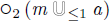 and
and  by fresh atoms and then adds extra formulas that ensure the relationship between those and the formulas they replace. Although the proof strategy is to proceed by structural induction, it is not directly possible here since, for instance,
  is not a proper subformula of
  . We aim to define a well-founded strict partial order that takes into account not only the complexity of the input formula but also the unfolding of the
  ,
,  ,
, $\mathbin {\boldsymbol{\mathsf{S}}}_{\leq n}$
and
$\mathbin {\boldsymbol{\mathsf{S}}}_{\leq n}$
and $\mathbin {\boldsymbol{\mathsf{T}}}_{\leq n}$
operators. We associate with each metric temporal formula
$\mathbin {\boldsymbol{\mathsf{T}}}_{\leq n}$
operators. We associate with each metric temporal formula $\varphi$
a natural number
$\varphi$
a natural number $\mathit{u}(\varphi )$
that is used to define our well-founded strict partial order.
$\mathit{u}(\varphi )$
that is used to define our well-founded strict partial order.
Definition 6. For a given metric formula $\varphi$
in the language, we define
$\varphi$
in the language, we define $\mathit{u}(\varphi )$
, that captures the unfolding of the formulas
$\mathit{u}(\varphi )$
, that captures the unfolding of the formulas  ,
, $\varphi \mathbin {\boldsymbol{\mathsf{S}}}_{\leq n} \psi$
and
$\varphi \mathbin {\boldsymbol{\mathsf{S}}}_{\leq n} \psi$
and $\varphi \mathbin {\boldsymbol{\mathsf{T}}}_{\leq n} \psi$
, as follows:
$\varphi \mathbin {\boldsymbol{\mathsf{T}}}_{\leq n} \psi$
, as follows:
-
•
$\mathit{u}(\bot ) = \mathit{u}(\top ) = 1$
; -
•
$\mathit{u}(a) = 1$
, for all
$a \in \mathcal{A}$
; -
•
$\mathit{u}(\varphi \otimes \psi ) = 1 + \mathit{u}(\varphi ) + \mathit{u}(\psi )$
, with ; -
•
$\mathit{u}(\oplus \varphi ) = 1+\mathit{u}(\varphi )$
, with
$\oplus \in \lbrace \unicode{x25EF}$
,
$\unicode{x2B24}$
,
$\widehat {\unicode{x25EF}}$
,
$\widehat {\unicode{x2B24}}$
,
$\unicode{x25EF}_{I}$
,
$\unicode{x2B24}_{I}$
,
$\widehat {\unicode{x25EF}}_{I}$
,
$\widehat {\unicode{x2B24}}_{I}$
,
$\Diamond$
,
$\blacklozenge$
,
$\square$
,
$\blacksquare$
$\rbrace$
; -
•
$\mathit{u}(\varphi \otimes _{\leq n} \psi ) = 2*(n+1)+\mathit{u}(\varphi ) + \mathit{u}(\psi )$
, with ; -
•
$\mathit{u}(\oplus _{\leq n} \varphi )= 2*(n+1)+\mathit{u}(\varphi )$
, with
$\oplus \in \lbrace \Diamond$
,
$\blacklozenge$
,
$\square$
,
$\blacksquare$
$\rbrace$
.




 ;
;



 ;
;


Given two metric formulas, we say that $\varphi \prec _{\mathit{u}} \psi$
if and only if
$\varphi \prec _{\mathit{u}} \psi$
if and only if $\mathit{u}(\varphi ) \lt \mathit{u}(\psi )$
. Since the previous definition is given as a mapping into the natural numbers, we can readily prove the following result.
$\mathit{u}(\varphi ) \lt \mathit{u}(\psi )$
. Since the previous definition is given as a mapping into the natural numbers, we can readily prove the following result.
Proposition 5. $\prec _{\mathit{u}}$
is a well-founded strict partial order.
$\prec _{\mathit{u}}$
is a well-founded strict partial order.
Regarding our running example, we get  ,
,  , and
, and  . Consequently,
  ,
,  and
and  , which allows us to apply the induction on the unfolding of binary metric temporal operators. Thanks to Proposition 5, we can use $\mathit{u}$
to provide an induction hypothesis, which is not based on the typical structural induction.
$\mathit{u}$
to provide an induction hypothesis, which is not based on the typical structural induction.
The following theorem states that an arbitrary metric temporal formula $\varphi$
Footnote
4
over an alphabet
$\varphi$
Footnote
4
over an alphabet $\mathcal{A}$
can be compiled into a metric temporal logic program
$\mathcal{A}$
can be compiled into a metric temporal logic program $\Gamma$
over an extended alphabet
$\Gamma$
over an extended alphabet $\mathcal{A}_{{\ell _{}}}\supseteq \mathcal{A}$
in such a way that there exists a bijection between the timed
$\mathcal{A}_{{\ell _{}}}\supseteq \mathcal{A}$
in such a way that there exists a bijection between the timed $\textrm {HT}$
-traces of length
$\textrm {HT}$
-traces of length $\lambda \in [1..\omega )$
satisfying
$\lambda \in [1..\omega )$
satisfying $\varphi$
and the traces of length
$\varphi$
and the traces of length $\lambda$
satisfying
$\lambda$
satisfying $\Gamma$
projected onto
$\Gamma$
projected onto $\mathcal{A}$
. That is, we have equivalence modulo auxiliary atoms.
$\mathcal{A}$
. That is, we have equivalence modulo auxiliary atoms.
Theorem 1 (Metric temporal logic program reduction).
For every metric temporal formula $\varphi$
4 over
$\varphi$
4 over $\mathcal{A}$
and for any
$\mathcal{A}$
and for any $\lambda \in [1..\omega )$
, we have that
$\lambda \in [1..\omega )$
, we have that
 \begin{equation} \textrm {MHT}(\varphi ,\lambda ) = \lbrace \mathbf{M}|_{\mathcal{A}} \mid \mathbf{M} \in \textrm {MHT}(\lbrace {\ell _{\varphi }} \rbrace \cup \eta ^*(\varphi ), \lambda ) \rbrace . \end{equation}
For transforming arbitrary temporal formulas into metric temporal logic programs, we use a Tseitin-style reduction (Tseitin Reference Tseitin1968) that relies on an alphabet extended by new atoms for each formula in the original language. The equivalence result in Theorem 1 is then obtained after removing auxiliary atoms and, in fact, is still preserved inside the context of a larger theory for the original vocabulary. The results presented in Theorem 1 are preserved when selecting the minimal models. This means that there exists a bijection between the metric equilibrium models of $\varphi$
and
$\varphi$
and $\Gamma$
projected onto
$\Gamma$
projected onto $\mathcal{A}$
. That is, we have strong equivalence modulo auxiliary atoms.
$\mathcal{A}$
. That is, we have strong equivalence modulo auxiliary atoms.
Corollary 2. For every metric temporal formula $\varphi$
4 over
$\varphi$
4 over $\mathcal{A}$
, for any
$\mathcal{A}$
, for any $\lambda \in [1..\omega )$
and any theory
$\lambda \in [1..\omega )$
and any theory $\Gamma$
over
$\Gamma$
over $\mathcal{A}$
,
$\mathcal{A}$
,
 \begin{equation} \textrm {MEL}(\lbrace \varphi \rbrace \cup \Gamma ,\lambda ) = \{\langle (\mathbf{H},\mathbf{T}),\tau \rangle |_{\mathcal{A}} \mid \langle (\mathbf{H},\mathbf{T}),\tau \rangle \in \textrm {MEL}(\lbrace {\ell _{\varphi }} \rbrace \cup \eta ^*(\varphi ) \cup \Gamma ,\lambda )\}. \end{equation}
Theorem 1 and Corollary 2 can be extended to arbitrary theories by defining the translation $\sigma$
as the metric temporal logic program:
$\sigma$
as the metric temporal logic program:
 \begin{align*} \sigma (\Gamma ) = \left \lbrace {\ell _{\gamma }} \mid \gamma \in \Gamma \right \rbrace \cup \left \lbrace \eta ^*(\mu ) \mid \mu \in cl(\Gamma )\right \rbrace \end{align*}
and then replacing $\lbrace {\ell _{\varphi }} \rbrace \cup \eta ^*(\varphi )$
by
$\lbrace {\ell _{\varphi }} \rbrace \cup \eta ^*(\varphi )$
by $\sigma (\Gamma )$
in expressions (9) and (10). Table 4 shows the translation of the expression in (1), which is done by applying the translation
$\sigma (\Gamma )$
in expressions (9) and (10). Table 4 shows the translation of the expression in (1), which is done by applying the translation $\eta (\mu )$
for each
$\eta (\mu )$
for each $\mu \in \mathit{cl}$
((1)). A metric temporal logic program can be obtained by using
$\mu \in \mathit{cl}$
((1)). A metric temporal logic program can be obtained by using $\eta ^*(\mu )$
instead. The rest of this section is devoted to proving Theorem 1, for which we extend Cabalar’s reduction for the case
$\eta ^*(\mu )$
instead. The rest of this section is devoted to proving Theorem 1, for which we extend Cabalar’s reduction for the case $\textrm {THT}_{\!\omega }$
(Cabalar Reference Cabalar, Janhunen and Niemelä2010) to the case of
$\textrm {THT}_{\!\omega }$
(Cabalar Reference Cabalar, Janhunen and Niemelä2010) to the case of $\textrm {MHT}_{\!f}$
. The reduction uses an extended alphabet
$\textrm {MHT}_{\!f}$
. The reduction uses an extended alphabet $\mathcal{A}_{{\ell _{}}}\supseteq \mathcal{A}$
that additionally contains a new atom
$\mathcal{A}_{{\ell _{}}}\supseteq \mathcal{A}$
that additionally contains a new atom $\ell _{\varphi }$
(aka label) for each formula
$\ell _{\varphi }$
(aka label) for each formula $\varphi$
in the original language over
$\varphi$
in the original language over $\mathcal{A}$
. For convenience, we use
$\mathcal{A}$
. For convenience, we use ${\ell _{\varphi }} \overset {\mathit{def}}{=} \varphi$
if
${\ell _{\varphi }} \overset {\mathit{def}}{=} \varphi$
if $\varphi$
is
$\varphi$
is $\top , \bot$
or an atom
$\top , \bot$
or an atom $a \in \mathcal{A}$
. For any non-atomic formula
$a \in \mathcal{A}$
. For any non-atomic formula $\gamma$
over
$\gamma$
over $\mathcal{A}$
, we introduce the translation
$\mathcal{A}$
, we introduce the translation $\eta$
given along Tables 1, 2, and 3, and call
$\eta$
given along Tables 1, 2, and 3, and call $\eta (\gamma )$
the definition of
$\eta (\gamma )$
the definition of $\gamma$
(the translation rules for Boolean and non-metric operators are provided in Tables A1 and A2). This definition is not a logic program yet, but it contains some double implication that can be easily transformed into a metric temporal logic program format by simple, non-modal transformations in the propositional logic of
$\gamma$
(the translation rules for Boolean and non-metric operators are provided in Tables A1 and A2). This definition is not a logic program yet, but it contains some double implication that can be easily transformed into a metric temporal logic program format by simple, non-modal transformations in the propositional logic of $\textrm {HT}$
. This translation of
$\textrm {HT}$
. This translation of $\eta (\mu )$
into a metric temporal logic program is shown in the tables as
$\eta (\mu )$
into a metric temporal logic program is shown in the tables as $\eta ^*(\mu )$
. In the rest of the section, we indistinctly use
$\eta ^*(\mu )$
. In the rest of the section, we indistinctly use $\eta (\mu )$
and
$\eta (\mu )$
and $\eta ^*(\mu )$
, as the former is more suitable for developing the proofs. As said before, their equivalence can be easily tested inside logic HT, and so, is not provided in this paper.
$\eta ^*(\mu )$
, as the former is more suitable for developing the proofs. As said before, their equivalence can be easily tested inside logic HT, and so, is not provided in this paper.
Translation for metric next, weak next, previous and weak previous

Table 1. Long description
The table has four rows and three columns. The columns are labeled with mu, eta(μ), and η*(μ). The rows are labeled with φ, φ subscript I, Iφ, and Iφ subscript I. Each cell contains specific logical expressions and their translations. Row 1: μ: φ, η(μ): hat O box (bullet T arrow right bullet (lμ arrow left lφ)), hat O diamond (bullet T arrow right bullet lμ), box (F arrow right lμ), η*(μ): hat O box (bullet lμ arrow right lφ), hat O diamond (bullet T land lφ arrow right bullet lμ), hat O diamond (bullet T arrow right bullet lμ), box (F arrow right lμ). Row 2: μ: φ subscript I, η(μ): hat O box (bullet T arrow right bullet (lμ arrow left lφ)), hat O diamond (bullet T arrow right bullet lμ), box (F arrow right lμ), η*(μ): hat O box (bullet lμ arrow right lφ), hat O diamond (bullet T land lφ arrow right bullet lμ), hat O diamond (bullet T arrow right bullet lμ), box (F arrow right lμ). Row 3: μ: Iφ, η(μ): hat O diamond (lμ arrow right I lφ), arrow right lμ, η*(μ): hat O box (lμ arrow right I lφ), hat O diamond (I lφ arrow right lμ), arrow right lμ. Row 4: μ: Iφ subscript I, η(μ): hat O box (lμ arrow right hat I lφ), lμ, η*(μ): hat O box (lμ land T arrow right lφ), hat O diamond (I lφ arrow right lμ), lμ.
Translation of metric since and metric trigger
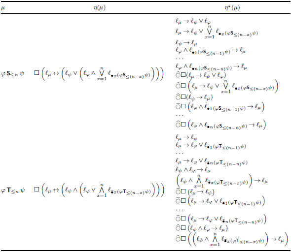
Table 2. Long description
The table presents translations of metric temporal logic expressions. It includes two main columns labeled eta(mu) and eta*(mu), each containing various logical expressions. The expressions involve logical operators such as implication, conjunction, disjunction, and negation, along with temporal operators like next, previous, since, and trigger. The table is divided into two sections, each with multiple rows of logical formulas. The first section starts with the expression phi subscript S less than or equal to n psi and translates it into a series of implications involving temporal operators. The second section starts with the expression phi subscript T less than or equal to n psi and similarly translates it into a series of implications involving temporal operators. Each row in the table shows a different logical expression and its corresponding translation.
Translation of metric until and metric release

Table 3. Long description
The table presents translations of metric temporal logic expressions. It includes two main sections, each with a formula and its corresponding translations. The first section shows translations for metric next, weak next, previous, and weak previous. The second section shows translations for metric since and metric trigger. Each section includes multiple rows with different translations, indicated by symbols such as ‘ell’, ‘ell subscript psi’, ‘ell subscript phi’, and various logical operators. The translations are presented in a structured format with clear labeling and logical expressions.
Translation of (1) into a metric temporal logic program. Equivalences of the form ${\ell _{\varphi }}\leftrightarrow p$
, with
${\ell _{\varphi }}\leftrightarrow p$
, with $p\in \mathcal{A}$
, are not shown and
$p\in \mathcal{A}$
, are not shown and $p$
is used instead of
$p$
is used instead of $\ell _{p}$
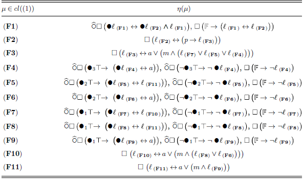
Table 4. Long description
An equation with multiple lines labeled from F1 to F11. Each line represents a different formula. The formulas include various logical operators such as diamonds, boxes, implications, and conjunctions. Variables and constants are used throughout the equations, with some lines containing nested logical expressions. The equations are structured to show the translation of a specific formula into a metric temporal logic program.
Given a trace $\mathbf{M}= \langle (\mathbf{H},\mathbf{T}),\tau \rangle$
of length
$\mathbf{M}= \langle (\mathbf{H},\mathbf{T}),\tau \rangle$
of length $\lambda \in \mathbb{N}\cup \lbrace \omega \rbrace$
, we define its projection onto the alphabet
$\lambda \in \mathbb{N}\cup \lbrace \omega \rbrace$
, we define its projection onto the alphabet $\mathcal{A}$
as
$\mathcal{A}$
as $\mathbf{M}\mid _{\mathcal{A}} = \langle (\mathbf{H}',\mathbf{T}'),\tau \rangle$
where
$\mathbf{M}\mid _{\mathcal{A}} = \langle (\mathbf{H}',\mathbf{T}'),\tau \rangle$
where $H'_i = H_i \cap \mathcal{A}$
and
$H'_i = H_i \cap \mathcal{A}$
and $T'_i = T_i \cap \mathcal{A}$
, for all
$T'_i = T_i \cap \mathcal{A}$
, for all $i \in [0..\lambda )$
.
$i \in [0..\lambda )$
.
Lemma 2. Let $\mathbf{M} = \langle (\mathbf{H},\mathbf{T}),\lambda \rangle$
be a
$\mathbf{M} = \langle (\mathbf{H},\mathbf{T}),\lambda \rangle$
be a $\textrm {MHT}$
model of length
$\textrm {MHT}$
model of length $\lambda \in [1..\omega )$
of a formula
$\lambda \in [1..\omega )$
of a formula $\varphi$
over
$\varphi$
over $\mathcal{A}$
. Then, there exists some timed
$\mathcal{A}$
. Then, there exists some timed $\textrm {HT}$
-trace
$\textrm {HT}$
-trace $\mathbf{M}'=\langle (\mathbf{H}',\mathbf{T}'),\tau \rangle$
over alphabet
$\mathbf{M}'=\langle (\mathbf{H}',\mathbf{T}'),\tau \rangle$
over alphabet $\mathcal{A}_{{\ell _{}}}$
such that
$\mathcal{A}_{{\ell _{}}}$
such that $\mathbf{M} = \mathbf{M}'|_{\mathcal{A}}$
and
$\mathbf{M} = \mathbf{M}'|_{\mathcal{A}}$
and $\mathbf{M}',0 \models \lbrace {\ell _{\varphi }} \rbrace \cup \eta ^*(\varphi )$
.
$\mathbf{M}',0 \models \lbrace {\ell _{\varphi }} \rbrace \cup \eta ^*(\varphi )$
.
Lemma 3. Let $\varphi$
be a temporal formula over
$\varphi$
be a temporal formula over $\mathcal{A}$
and let
$\mathcal{A}$
and let $\langle (\mathbf{H},\mathbf{T}),\tau \rangle$
be a
$\langle (\mathbf{H},\mathbf{T}),\tau \rangle$
be a $\textrm {MHT}$
model, with length
$\textrm {MHT}$
model, with length $\lambda \in [1..\omega )$
, of
$\lambda \in [1..\omega )$
, of $\lbrace {\ell _{\varphi }}\rbrace \cup \eta (\varphi )$
. Let
$\lbrace {\ell _{\varphi }}\rbrace \cup \eta (\varphi )$
. Let $\boldsymbol m$
be its associated three-valued interpretation. Then for any
$\boldsymbol m$
be its associated three-valued interpretation. Then for any $\mu \in cl(\varphi )$
and any
$\mu \in cl(\varphi )$
and any $k \in [0..\lambda )$
, we have
$k \in [0..\lambda )$
, we have $\boldsymbol{m}(k,{\ell _{\mu }}) = \boldsymbol{m}(k,\mu )$
.
$\boldsymbol{m}(k,{\ell _{\mu }}) = \boldsymbol{m}(k,\mu )$
.
Let us discuss now the proof of Theorem 1. We show that for any metric temporal formula $\varphi$
over
$\varphi$
over $\mathcal{A}$
and any
$\mathcal{A}$
and any $\lambda \in [1..\omega )$
,
$\lambda \in [1..\omega )$
,
 \begin{equation*} \textrm {MHT}(\varphi ,\lambda ) = \lbrace \mathbf{M}|_{\mathcal{A}} \mid \mathbf{M} \in \textrm {MHT}(\lbrace {\ell _{\varphi }} \rbrace \cup \eta (\varphi ), \lambda ) \rbrace . \end{equation*}
The ‘ $\subseteq$
’ direction follows from Lemma 2. For the ‘
$\subseteq$
’ direction follows from Lemma 2. For the ‘ $\supseteq$
’ direction, take some
$\supseteq$
’ direction, take some $\textrm {MHT}$
model
$\textrm {MHT}$
model $\mathbf{M}$
of
$\mathbf{M}$
of $\eta (\varphi )$
of length
$\eta (\varphi )$
of length $\lambda \in [1..\omega )$
. This implies that its associated
$\lambda \in [1..\omega )$
. This implies that its associated $3$
-valuation satisfies
$3$
-valuation satisfies ${\boldsymbol{m'}}(0,{\ell _{\varphi }})=2$
, which is included in
${\boldsymbol{m'}}(0,{\ell _{\varphi }})=2$
, which is included in $\eta (\varphi )$
. Since
$\eta (\varphi )$
. Since $\varphi \in cl(\varphi )$
, we can apply Lemma 3 to conclude
$\varphi \in cl(\varphi )$
, we can apply Lemma 3 to conclude ${\boldsymbol{m'}}(k,{\ell _{\varphi }})={\boldsymbol{m'}}(k,\varphi )$
for all
${\boldsymbol{m'}}(k,{\ell _{\varphi }})={\boldsymbol{m'}}(k,\varphi )$
for all $k \in [0..\lambda )$
but then, in particular,
$k \in [0..\lambda )$
but then, in particular, $2={\boldsymbol{m'}}(0,{\ell _{\varphi }})={\boldsymbol{m'}}(0,\varphi )$
and so,
$2={\boldsymbol{m'}}(0,{\ell _{\varphi }})={\boldsymbol{m'}}(0,\varphi )$
and so, $\mathbf{M}$
is also a model of
$\mathbf{M}$
is also a model of $\varphi$
. Finally,
$\varphi$
. Finally, $\mathbf{M}|_{\mathcal{A}}$
is still a model of
$\mathbf{M}|_{\mathcal{A}}$
is still a model of $\varphi$
because the latter is a theory over vocabulary
$\varphi$
because the latter is a theory over vocabulary $\mathcal{A}$
. The theorem below provides a parametric polynomial bound of the size of
$\mathcal{A}$
. The theorem below provides a parametric polynomial bound of the size of $\eta ^*(\varphi )$
.
$\eta ^*(\varphi )$
.
Theorem 2. The number of rules in $\eta ^*(\varphi )$
has a (parametric) polynomial bound that depends on
$\eta ^*(\varphi )$
has a (parametric) polynomial bound that depends on $n$
and
$n$
and $\lvert \varphi \rvert$
, where
$\lvert \varphi \rvert$
, where $n$
is the maximum interval value occurring in a subformula of
$n$
is the maximum interval value occurring in a subformula of $\varphi$
, which is of the form
$\varphi$
, which is of the form $Q_{\leq n}$
, where
$Q_{\leq n}$
, where  .
.
5 Conclusion
In this paper, we have described a Tseitin-like reduction from metric temporal logic formulas into a logic programming format under metric equilibrium logic semantics. Our current translation only considers intervals of the form $[0..n]$
in the binary metric operators since (resp. trigger) and until (resp. release). In the future, we expect to extend our translation in order to cope with arbitrary intervals. If that is possible, we would have an input format to which any arbitrary metric temporal theory could be reduced, making it easily implementable in ASP.
$[0..n]$
in the binary metric operators since (resp. trigger) and until (resp. release). In the future, we expect to extend our translation in order to cope with arbitrary intervals. If that is possible, we would have an input format to which any arbitrary metric temporal theory could be reduced, making it easily implementable in ASP.
Our contribution sheds light on the concept of metric temporal logic programs and its use as a “normal form” for interpreting metric temporal theories under answer set semantics. As future work, we expect to implement this translation in the solver telingo (Cabalar et al. Reference Cabalar, Kaminski, Morkisch, Schaub, Balduccini, Lierler and Woltran2019) and compare it with other solvers proposed by Becker et al. (Reference Becker, Cabalar, Diéguez, Hahn, Romero and Schaub2024a, Reference Becker, Cabalar, Diéguez, Hahn, Romero and Schaub2026). In addition, we would like to explore the notion of splittable metric temporal logic programs as done by Aguado et al. (Reference Aguado, Cabalar, Diéguez, Pérez, Schaub, Schuhmann and Vidal2023) for $\textrm {TEL}$
. In the temporal case, those programs possess nice computational methods via the use of splitting and loop formulas. An interesting research line could be to extend those results to the metric case. Finally, we would like to extend our reduction to metric extensions of dynamic equilibrium logic (Becker et al. Reference Becker, Cabalar, Diéguez, del Cerro, Schaub and Schuhmann2023)
$\textrm {TEL}$
. In the temporal case, those programs possess nice computational methods via the use of splitting and loop formulas. An interesting research line could be to extend those results to the metric case. Finally, we would like to extend our reduction to metric extensions of dynamic equilibrium logic (Becker et al. Reference Becker, Cabalar, Diéguez, del Cerro, Schaub and Schuhmann2023)
Appendix A Translation of Non-Metric Connectives
Translation of the propositional connectives
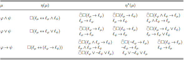
Table A1. Long description
The table presents translations of propositional connectives into metric temporal logic. It includes various logical expressions and their corresponding translations. Each row represents a different connective or logical operation, with columns showing the original expression and its translation. The table is divided into sections for different types of connectives, such as next, previous, since, and trigger operations. Each section provides specific translations for metric, weak, and other variants of these operations.
Translation of the non-metric temporal operators

Table A2. Long description
The table is divided into three columns labeled mu, eta(mu), and eta*(mu). Each row corresponds to a different temporal operator or combination of operators. The first column lists the original temporal operators, including next, previous, since, trigger, and their weak versions. The second column shows the translation of these operators into metric temporal logic programs using the eta function. The third column presents the translation using the eta* function. Each cell in the table contains a logical expression representing the translation of the corresponding operator.


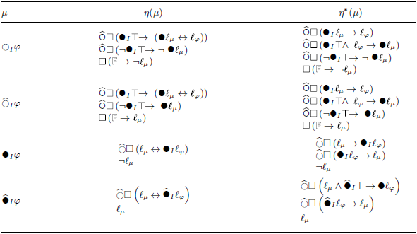
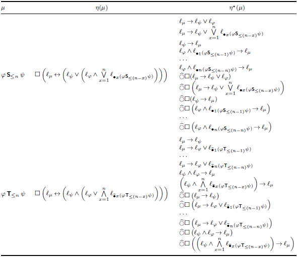
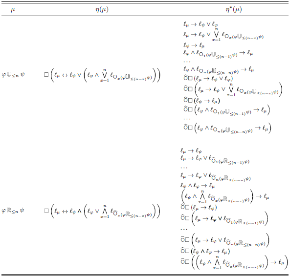
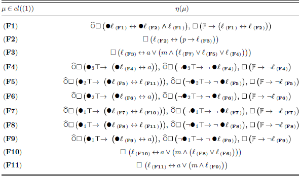
 ℓφ↔p
ℓφ↔p p∈A
p∈A p
p ℓp
ℓp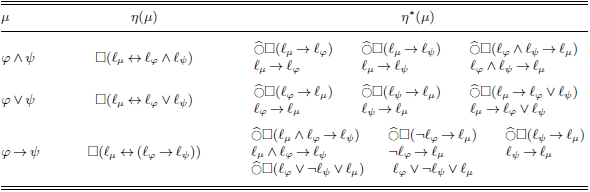
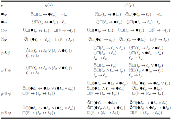

 Open access

