


1. Introduction
Warming of Arctic regions in recent decades has taken place at far faster rates than the rest of the world (Rantanen and others, Reference Rantanen2022). This process of Arctic amplification has been felt in the Canadian Arctic where environmental and climatic changes are proceeding at rates that are amongst the fastest of any region on earth (Bush and Lemmen, Reference Bush and Lemmen2019; Cooley and others, Reference Cooley2020). One of the most striking of such climate-driven environmental changes is the retreat of glaciers, ice caps and ice sheets (Cook and others, Reference Cook2019; Hugonnet and others, Reference Hugonnet2021; Menounos and others, Reference Menounos, Huss, Marshall, Ednie, Florentine and Hartl2025). The ice cover of the Canadian Arctic accounts for one-third of all land ice outside of the major ice sheets of Antarctica and Greenland, and negative glacier mass balance across the Canadian Arctic Archipelago was a major contributor to the sea-level rise experienced in the early years of the present century (Gardner and others, Reference Gardner2011, Reference Gardner, Moholdt, Arendt and Wouters2012; Gilbert and others, Reference Gilbert2016). Since the late 1990s melt from the ice of the Canadian Arctic has occurred at rates that are higher than at any point in the past 4000 years (Gardner and others, Reference Gardner, Moholdt, Arendt and Wouters2012; Bash and Moorman, Reference Bash and Moorman2020), and model projections suggest that Arctic Canada will continue to be the most significant of all the mountain glacier contributors to sea-level rise up until the end of the 21st century (Radić and Hock, Reference Radić and Hock2011). It is therefore important to gain a better understanding of how these glaciers and ice caps lose mass in response to the warming climate. Given the significant component of Canadian ice mass lost through the melting of ice at the surface, a highly developed understanding of the controls on meltwater generation and transport is also important (Bash and Moorman, Reference Bash and Moorman2020).
As a consequence of increasing atmospheric temperatures, the amount of melt generated on the majority of glaciers worldwide is increasing. Throughout the Arctic, rising equilibrium line altitudes (ELA) over the next few decades are projected to result in the greater exposure of bare ice during the melt season, tracking broader trends of glacier thinning and retreat (Huss and Hock, Reference Huss and Hock2015; Ryan and others, Reference Ryan2019; Irvine-Fynn and others, Reference Irvine-Fynn2022). Subsequent melting of ice in these regions generates surface water. On the Greenland Ice Sheet (GrIS)—the largest body of ice outside of Antarctica, and where rapid change is visible—there has been an exceptional rise in meltwater runoff over the last two decades (Trusel and others, Reference Trusel2018), which has resulted in the development of many thousands of large supraglacial lakes on the ice surface each summer (e.g. Leeson and others, Reference Leeson, Shepherd, Palmer, Sundal and Fettweis2012, Reference Leeson2015; Selmes and others, Reference Selmes, Murray and James2011; Sundal and others, Reference Sundal, Shepherd, Nienow, Hanna, Palmer and Huybrechts2009; Otto and others, Reference Otto, Holmes and Kirchner2022). In addition, extremely extensive networks of supraglacial channels develop, transporting large volumes of water great distances across the ice sheet.
The conventional understanding is that during the summer melt season, meltwater is generated at the ice surface. Where snow persists at the surface, some of this meltwater might percolate through the snowpack and refreeze. When meltwater is generated on ice (or reaches ice after passing through snow), it is conveyed through a network of supraglacial channels. These channels are frequently interrupted by crevasses and moulins, diverting water into the glacier itself, where it encounters englacial and/or subglacial drainage systems which can vary greatly in structure and efficiency (Pitcher and Smith, Reference Pitcher and Smith2019). As a result, the residency time of meltwater within the whole glacier system can differ greatly between glaciers and throughout the melt season; however, this meltwater will ultimately reach the glacier margin and proglacial zone, constituting mass loss. Considering just the supraglacial component of the drainage system, the combined effect of this drainage network, consisting of supraglacial lakes and channels, not only enables the storage and evacuation of meltwater here, but impacts surface albedo, and thus creates positive feedbacks with the meltwater-generation cycle (Stroeve, Reference Stroeve2001; McCutcheon and others, 2021).
The broad spatial structure of large supraglacial drainage systems is thought to primarily be controlled by the topography of the ice surface, which at least to some degree is controlled by the shape of the underlying topography (Karlstrom and Yang, Reference Karlstrom and Yang2016; Rawlins and others, Reference Rawlins, Rippin, Sole, Livingstone and Yang2023). Large-scale topographic variations at the bed are transmitted to the surface and these determine the broad structure of supraglacial drainage networks (Yang and others, Reference Yang, Smith, Chu, Gleason and Li2015; Lu and others, Reference Lu2020). However, due to the thermo-mechanical erosive power of cold flowing water, the relatively high erodibility of ice, and the changing volume of available water, channels and drainage networks evolve substantially over the course of a melt season, and most likely between melt seasons too as a result of these processes (Irvine-Fynn and others, Reference Irvine-Fynn, Hodson, Moorman, Vatne and Hubbard2011; Lampkin and Vanderberg, Reference Lampkin and Vanderberg2014; Lu and others, Reference Lu2020). Consequently, the dynamic nature of the supraglacial hydrological network itself exerts significant influence on the topography and roughness of the ice surface (Rippin and others, Reference Rippin, Pomfret and King2015; Irvine-Fynn and others, Reference Irvine-Fynn2022), alongside turbulent energy fluxes determined by the topography of the ice surface (Hock, Reference Hock2005; Irvine-Fynn and others, Reference Irvine-Fynn2022). Therefore, it seems that the complex interactions between supraglacial hydrology, topography and atmospheric energy exchanges are important when it comes to understanding hydrological drainage network evolution and the erosion and sculpting of the supraglacial landscape.
Despite the undoubted importance of drainage networks, it is only in the last two decades that supraglacial networks, particularly those of larger size and extent, have received significant attention, with the vast majority focussed on the ablating margins of the GrIS (Gleason and others, Reference Gleason2016; Lu and others, Reference Lu2020, Reference Lu2021; Otto and others, Reference Otto, Holmes and Kirchner2022; Rawlins and others, Reference Rawlins, Rippin, Sole, Livingstone and Yang2023; Smith and others, Reference Smith2015, 2017; Sundal and others, Reference Sundal, Shepherd, Nienow, Hanna, Palmer and Huybrechts2009; Yang and others, Reference Yang, Smith, Chu, Gleason and Li2015; Yang and others, Reference Yang, Smith, Chu, Pitcher, Gleason, Rennermalm and Li2016, Reference Yang2019, Reference Yang2021; Zhang and others, Reference Zhang2023). Extensive investigations have been carried out on the south and south-western margins of the GrIS (Joughin and others, Reference Joughin2013; Yang and Smith, Reference Yang and Smith2013; Lampkin and Vanderberg, Reference Lampkin and Vanderberg2014; Yang and others, Reference Yang, Smith, Chu, Gleason and Li2015, Reference Yang, Smith, Chu, Pitcher, Gleason, Rennermalm and Li2016, Reference Yang2019, Reference Yang2021; Glen and others, Reference Glen2025), documenting the spatial and temporal evolution of these networks, broadly highlighting how, over time, they have become larger, more persistent and more extensive as a response to the increasing volume of meltwater generation driven by climate change. Warming air temperatures and extreme melt years have facilitated the inland expansion of the GrIS ablation zone and subsequent supraglacial drainage network to progressively higher elevations, thereby extending their coverage across larger areas of the ice sheet (Otto and others, Reference Otto, Holmes and Kirchner2022; Rawlins and others, Reference Rawlins, Rippin, Sole, Livingstone and Yang2023; Zhang and others, Reference Zhang2023; Fan and others, Reference Fan, Ke, Luo, Shen, Livingstone and Lea2025; Glen and others, Reference Glen2025).
In the Canadian Arctic, despite the extensive ice cover and significant changes in recent decades, there are relatively few direct measurements of glacier melt and drainage processes (Bash and Moorman, Reference Bash and Moorman2020). Lu and others (Reference Lu2020) explored the Devon Ice Cap in the Canadian Arctic and noted that, as in Greenland, supraglacial drainage density typically increases through the melt season, reaching higher elevations as melt progresses and ablation peaks (Rawlins and others, Reference Rawlins, Rippin, Sole, Livingstone and Yang2023). Yang and others (Reference Yang2019) also explored drainage networks over small regions of both the Devon and Barnes Ice Caps (as well as Greenland), noting extensive channel networks, but such observations were made based on imagery from just a single day (Devon Ice Cap), or 2 days (NW Greenland Ice Sheet and Barnes Ice Cap), and so there was no consideration of more extensive temporal evolution. Further work on the Devon Ice Cap by Clason and others (Reference Clason, Mair, Burgess and Nienow2012) revealed the importance of an expanding and evolving supraglacial drainage network. The presence of greater amounts of surface water has the potential to influence the transfer of water from supraglacial to subglacial environments, with consequent impacts on basal sliding and thus overall ice dynamics (Clason and others, Reference Clason, Mair, Burgess and Nienow2012). With increasingly large volumes of surface meltwater driven by an increasingly warm world, we might also expect to see longer-term co-evolving changes in the surface topography and nature of supraglacial channel networks (size, extent, density, depth, etc.).
Here, we are interested in exploring how supraglacial drainage networks on the relatively understudied Barnes Ice Cap have evolved over timescales greater than just a few days (cf. Yang and others, Reference Yang2019), inducing changes to the topographic form driven by both ablation and the flow of water over the ice surface. We hypothesise that because of the increasing amount of meltwater generated, channel incision generates an increasingly topographically varied surface (Karlstrom and Yang, Reference Karlstrom and Yang2016). Conversely, increasing rates of widespread atmosphere-driven surface ablation may induce a reduction in surface variability due to overall ice surface lowering (Ryan and others, Reference Ryan2019; Irvine-Fynn and others, Reference Irvine-Fynn2022). The relative variability of an ice surface is thus a consequence of the battle between these two opposing processes. As a result, we would expect to see a highly variable and changeable supraglacial drainage network. Our intention is to explore this potential conflict and to focus our attention on the Barnes Ice Cap of Arctic Canada.
The overarching aim of this work is to track the hypothesised expansion of the supraglacial drainage network on the Barnes Ice Cap and its role in changes of the ice mass, both in the past, and considering the implications of this expansion into the future. In order to achieve this, we first explore changes in the geometry of the ice cap before investigating changes in the drainage network. Changes in the ice cap itself are important to consider, given it is the water generated by increasing surface melting that directly influences the form and nature of supraglacial drainage networks. We tackle all this via the following objectives:
1) To map changes in the ice cap as long as Landsat records allow.
2) To map the drainage network across the Barnes Ice Cap in Landsat imagery as long as the record allows.
3) To explore and quantify any changes in drainage network coverage, density and distribution over time.
4) To explore higher-resolution datasets (i.e. than the 30 m of Landsat) to map finer-scale drainage networks not otherwise visible in Landsat imagery.
2. Study location
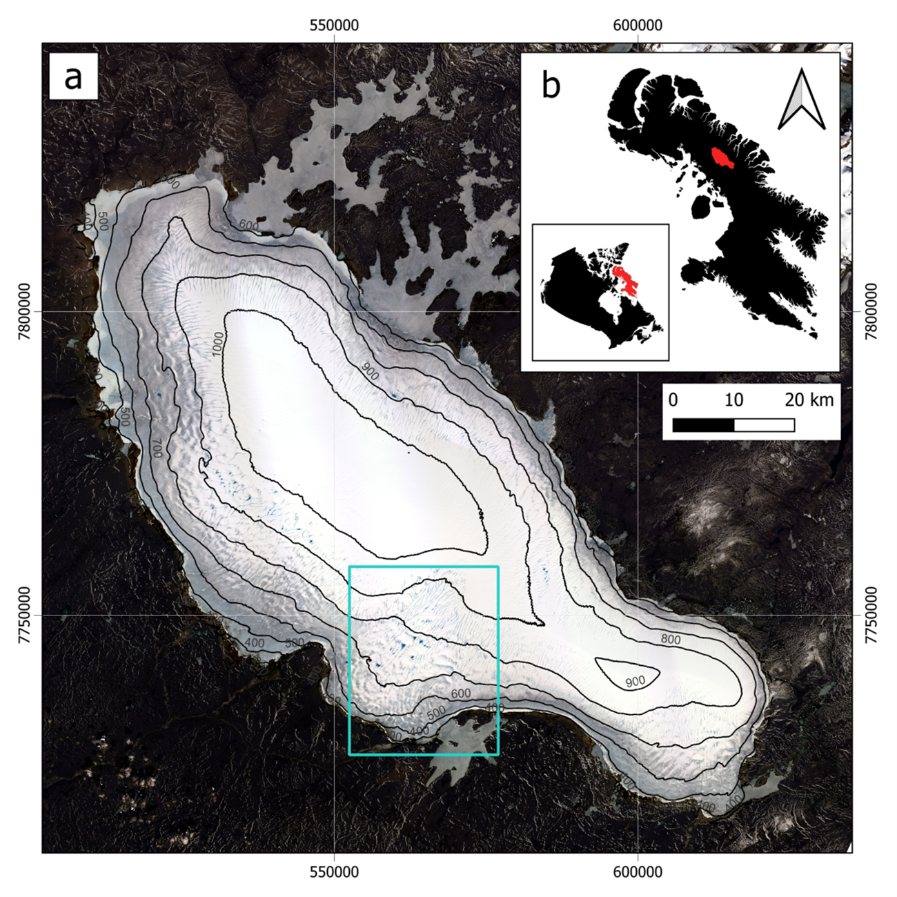
The Barnes Ice Cap is found in the centre of Baffin Island in Arctic Canada at a latitude of approximately 70°N (Fig. 1). In 2021, we measure the Barnes Ice Cap to cover an area of 5731 km2 while Gilbert (Reference Gilbert2016) reports a maximum thickness of ∼730 m. The ice cap was thought to be in balance towards the end of the 19th century but has experienced negative mass balance since that time, with an increasing rate of negative mass balance since the mid-1990s (Abdalati and others, Reference Abdalati2004; Sneed and others, Reference Sneed, Hooke and Hamilton2008; Gardner and others, Reference Gardner, Moholdt, Arendt and Wouters2012; Gilbert and others, Reference Gilbert2016, Reference Gilbert, Flowers, Miller, Refsnider, Young and Radić2017). Due to rising equilibrium lines, the Barnes Ice Cap lost its accumulation zone around the year 2010 (Gray and others, Reference Gray, Burgess, Copland, Demuth, Dunse, Langley and Schuler2015; Gilbert and others, Reference Gilbert2016, Reference Gilbert, Flowers, Miller, Refsnider, Young and Radić2017). At this rate, it is forecast to disappear within the next 300 years (Gilbert and others, Reference Gilbert, Flowers, Miller, Refsnider, Young and Radić2017). This loss will be permanent, even under a return to pre-industrial conditions, as the Barnes Ice Cap is a remnant of the Laurentide Ice Sheet (Gilbert and others, Reference Gilbert2016): the low-lying terrain and relatively high equilibrium line altitude mean that any loss of the ice cap is subject to hysteresis behaviour, requiring a return of glacial conditions to regrow to the pre-industrial extent.
(A) Landsat 8 image mosaic from 9 July 2022 of the Barnes Ice Cap on Baffin Island, Arctic Canada (band combination 4, 3, 2 in RGB; 100 m contours over the ice cap are derived from the 2 m ArcticDEM (Porter and others, Reference Porter2023)). The turquoise rectangle defines the area of interest in this study which we refer to as the central-southern outlet of the Barnes Ice Cap. (B) Baffin Island with the Barnes Ice Cap shown in red, and the inset to this inset shows Canada with Baffin Island marked in red. All components are in a UTM projection (zone 18 N).

Our study region comprises the central-southern outlet of the Barnes Ice Cap (see Fig. 1). This region covers much of a sector that was identified by Holdsworth (Reference Holdsworth1977) to have surged at some point in the past (an occurrence he noted based on the presence primarily of surge-scars), perhaps leading to a maximum extent around the year 1700. ITS_LIVE ice surface velocity data (see Fig. 6) indicates this to be the fastest-flowing sector of the ice cap, making it of particular interest when considering the interaction between surface water generation and ice dynamics. Finally, as an area of wider interest, this region includes margins of the ice cap that are lake-terminating and margins that are not, thus offering important insights into the differing impacts of terminal lakes on ice cap change.
3. Methods
3.1. Changes in glacier geometry
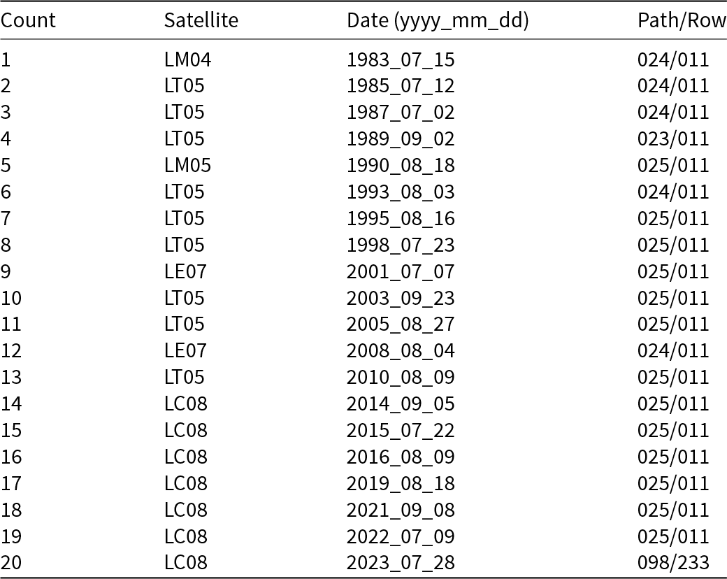
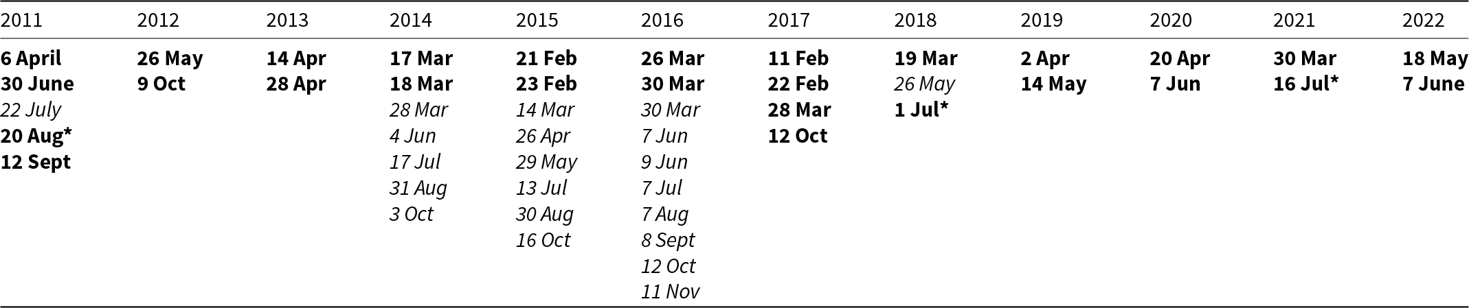
In order to achieve the stated aims, a series of Landsat Collection 2, Level 1 imagery were downloaded using the USGS facility Earth Explorer (https://earthexplorer.usgs.gov/). We obtained an annual image over as much of the Landsat record as possible, targeting the summer months to minimise snow cover, while also minimising cloud cover (Table 1). In some years, due to limited availability of imagery, snow cover was sometimes unavoidable. We also avoided Landsat 7 imagery where possible in the post-2003 period to minimise the need to utilise imagery impacted by the failure of the Scan Line Corrector (SLC).
Summary of dates over which imagery was downloaded and subsequently explored, as well as an indication of the satellite platform (i.e. Landsat 4 to 8) and the relevant path/row used, so as to assist any reader wishing to locate imagery.

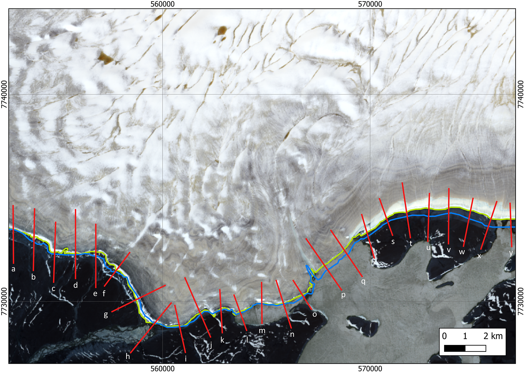
The next step involved quantifying the magnitude of change along the front of the Barnes Ice Cap in the region studied. This was done by manually digitising the ice front in each year. Band ratio classification approaches were explored, but still ultimately required laborious manual intervention to properly set ratio thresholds due to inconsistent identification of ice boundaries from one image to the next. Consequently, we determined a fully-manual approach to be preferable for delineating the ice margin. Due to the size of the ice front over our area of interest, and the varying nature of the terminus we assessed frontal change at 25 separate locations to uncover any potential variability in glacier frontal change (Fig. 2).
Location of 25 separate locations (labelled a–y) where ice front change was measured over 20 different time-steps from 1983 to 2023 (see Table 1) along the terminus of the central–southern outlet study region. Measurement locations are marked with red lines, each orientated approximately perpendicular to the ice front and parallel to ice flow. The blue outline marks the position of the ice-front as determined from a Landsat-4 image from July 1983, while the green outline denotes the position of the ice-front as determined from a Landsat-8 image from July 2023. The background image is a Landsat 8 image from 28 July 2023 (band combination 4, 3, 2). Note that much of the eastern part of this region of the ice front is water terminating, but the western part is land-terminating.

The next stage of analysis was to investigate changes in surface elevation through an exploration of the Advanced Spaceborne Thermal Emission and Reflection Radiometer (ASTER) digital elevation models (DEM)-difference product (hereafter dDEMs) generated by Hugonnet and others (Reference Hugonnet2021) at a resolution of 100 m. This uses largely untapped ASTER imagery to provide global estimates of DEM-difference change at 5-year timesteps between 2000 and 2019/20, validated against other high precision instruments. The Barnes Ice Cap lies in the region identified as Arctic Canada South and here, over the 2000–2019 period, overall mean elevation change rates were −0.77 ± 0.06 m a−1.
3.2. Changes in the drainage network
To explore supraglacial drainage networks, we used two approaches. Firstly, we explored temporal change in supraglacial drainage networks using ArcticDEM strip data (Porter and others, Reference Porter2022), 2 m resolution stereoscopic DEMs acquired between 2007 and 2023. We selected two strips that covered this central-southern outlet study region (20 August 2011 and 20 April 2020), which overlapped with each other with minimal apparent artefacts. We downloaded and coregistered these strips using the pdemtools software package (Chudley & Howat, Reference Chudley and Howat2024), and within this, coregistered the strips against the ArcticDEM mosaic using exposed bedrock following Nuth and Kääb (Reference Nuth and Kääb2011). Where no exposed bedrock was available for coregistration against the ArcticDEM mosaic, we instead coregistered using contemporaneous ICESat-2 data (no greater the ±45 days from the strip date), downloaded via the sliderule software package (Shean and others, 2023). Although these strips did not cover our entire area of interest, the substantial zone of overlap allowed us to assess temporal changes over the majority of the tongue.
We quantitatively delineated stream distribution from our DEMs, using the QGIS tool r.stream.extract. This calculated hydrological flow direction and accumulation from topography. We prepared the DEMs by filling depressions that might arise due to artefacts. Flow direction was then computed using a single flow direction approach (sometimes known as the D8 algorithm). Using this approach, water from one cell flows into just one downstream cell—which cell was determined by computing a gradient between the source cell and the surrounding eight cells, with water flowing to the downstream cell with the steepest gradient. The result of this procedure was a flow direction raster. Flow accumulation was subsequently calculated by using the flow direction raster to determine how many upstream cells contributed to a particular downstream cell. This produced a flow accumulation raster that identifies which cells receive the most contribution from upstream cells. Cells that had the greatest upstream contributing area were identified as river channels. This flow accumulation raster was then converted into a polyline displaying the network of channels.
The ArcticDEM strip dataset is limited in temporal extent and coverage. In order to utilise the wealth of satellite imagery to better explore the supraglacial drainage network at the Barnes Ice Cap across a longer time period (1985 to 2020), Landsat archival imagery via Google Earth Engine (GEE; Gorelick and others, Reference Gorelick, Hancher, Dixon, Ilyushchenko, Thau and Moore2017) was used to best map the presence of water (i.e. large-scale supraglacial channels and subsequent networks) on the surface of the Barnes Ice Cap at 5-year time-intervals. Whilst higher-resolution imagery, such as Sentinel-2 (10 m), is available and has been used in other supraglacial hydrologic studies (Yang and others, Reference Yang2019; Rawlins and others, Reference Rawlins, Rippin, Sole, Livingstone and Yang2023; Zhang and others, Reference Zhang2023) to map more detailed network configurations (i.e. both larger, primary channels and thinner, more transient channels), Landsat images with a 30 m resolution continues to provide valuable, broad-scale insights into drainage network configurations and larger channels, which transport the largest volumes of melt (Yang and others, Reference Yang2021).
To maximise image availability and reduce the influence of cloud cover over the Barnes Ice Cap, especially in earlier years of the time-series, 5-year mean NDWI composite images for eight time periods were generated between 1985 and 2020, These periods were: 1985–1989, 1990–1994, 1995–1999, 2000–2004, 2005–2009, 2010–2014, 2015–2019, 2020–2024. A total of 250 Landsat Tier 1 images (from Landsat 5, 7 and 8) were used across the full time series, with between 20 and 45 images per interval, depending on seasonal and mission-specific availability. While image density does vary slightly across intervals, particularly for Landsat 5 due to known differences in acquisition strategy, data continuity and cloud contamination (Zhang and others, Reference Zhang, Chen, Guo, Yi, Zeng and Li2022), the 5-year compositing approach helps to mitigate these inconsistencies and ensure each interval reflects the average melt season hydrological state. Such compositing-per-time-window approach has been widely adopted in similar mapping studies to support the representative multitemporal detection of surface water features on icy surfaces (Tuckett et al., Reference Tuckett, Ely, Sole, Lea, Livingstone, Jones and van Wessem2021; Bazilova and Kääb, Reference Bazilova and Kääb2022; Zhang et al., Reference Zhang, Chen, Guo, Yi, Zeng and Li2022).
For each period, all available Landsat Tier 1 imagery (Landsat 5, 7 and 8) from the typical melt season months of June to August was filtered to retain scenes with less than 20% cloud cover. NDWI was calculated using green and NIR bands (McFeeters, 1996) and mean NDWI values per pixel computed across the entire image collection to produce a single meltwater-enhanced composite image representative of each 5-year period. Mean NDWI was preferred over maximum to highlight consistently wet areas and provide a more stable representation of drainage features across time. These NDWI-composite images were then exported from GEE and processed in MATLAB using the well-documented automatic river detection algorithm by Yang and Smith (Reference Yang and Smith2012, Reference Yang, Smith, Chu, Gleason and Li2015). Variable thresholds for NDWI (between 0.1 and 0.32; Lu and others, Reference Lu2021) and Gabor-PPO processed images (10–20 out of 255) were selected via image histograms and visual inspection to extract supraglacial lakes and channels, respectively. Some manual cleaning was required in post-processing to assist with the joining of recurrently segmented channel sections, with the aid of RGB and NDWI GEE-generated images.
3.3. Surface velocity
Throughout our analysis, we were also concerned with investigating how surface dynamics influenced, or were influenced by, changes in ice geometry and/or hydrology. Surface velocities (m a−1) at 120 m spatial resolution were derived from the ITS_LIVE platform and were generated using auto-RIFT (Gardner and others, Reference Gardner2018) and provided by the NASA MEaSUREs ITS_LIVE project (Gardner and others, Reference Gardner, Fahnestock and Scambos2023; https://its-live.jpl.nasa.gov/).
4. Results
4.1. Glacier geometry
4.1.1. Changes in glacier extent
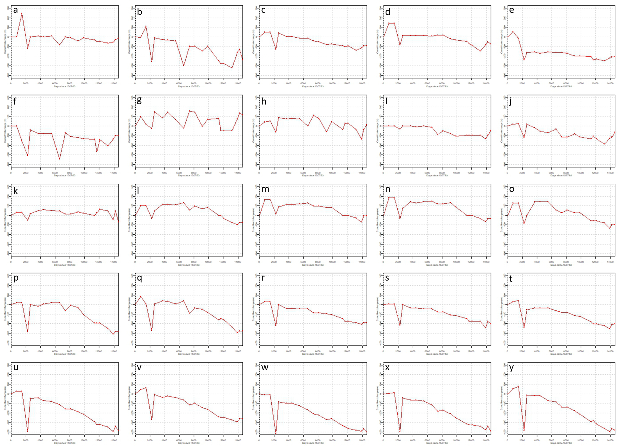
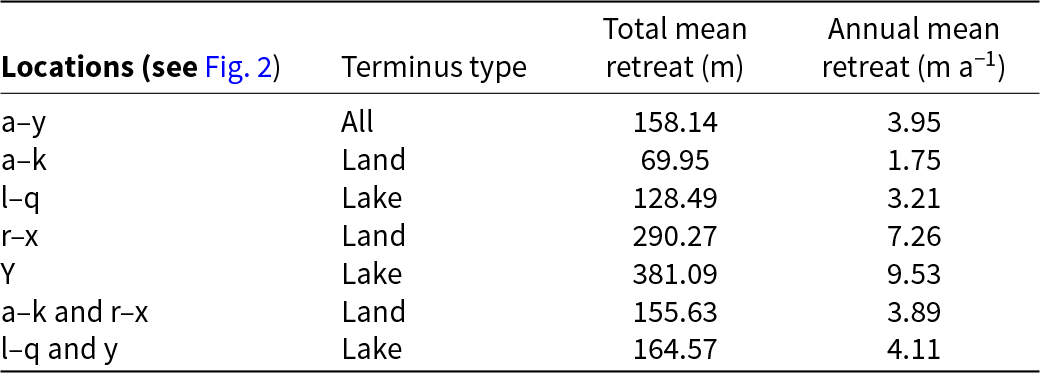
We show a high spatial variability in the pattern of frontal retreat over the 40-year study period (Fig. 3) across the 25 sites where retreat was measured (Fig. 2). Identifying the ice margins in 1983 and 2023 shows that retreat has been most extensive towards the eastern-side of the central-southern outlet study region (Fig. 2). Exploring temporal variability in retreat at the 25 study locations, the trend towards an increasing acceleration of ice front retreat is apparent (Fig. 3). The largest magnitude of retreat is identified in plots p–y representing the eastern-most measurement locations, which coincides with where the ice front partially terminates in proglacial lakes (Fig. 2 and Fig. 3). The locations where retreat is subdued or even relatively stable are found towards the western side of the area of investigation, where ice terminates on land (Fig. 3a-k). However, closer inspection of frontal change in Figs. 2 and 3 reveals that greater magnitudes of retreat are not always consistent with termination in water. Spatial variability is summarised in Table 2 in which we subdivide these sites up into land- and lake-terminating parts of the ice front. The average change over the 40-year period at all locations is a retreat of 158.14 m (3.95 m a−1) but the greatest retreat of 401 m (annual retreat rate of ∼10 m a−1) occurs at point w (Figs. 2 and 3; Table 2) which is a land-terminating location, while nearby point y is a rapidly retreating lake-terminating location. Clearly, there is great complexity in the behaviour of a retreating ice front, and while not the focus of this investigation, it does suggest that interactions with ice marginal water bodies might not be the only major driver of frontal retreat, as well as perhaps the nature of the basal topography.
Cumulative change in position of the ice front at 25 separate locations (see Figure 2) across the central–southern outlet study region of the Barnes Ice Cap. Measurements were made at 20 time-steps covering a 40-year period, between 15 July 1983 and 28 July 2023 (see Table 1). Each plot is labelled a–y so as to identify the position of each survey location. It is noticeable that virtually all plots show a retreating trend but there are fluctuations around this, with the most significant retreat being towards the right (east) of the study area, where the ice terminates in water. There is also a very marked step in retreat around day 2000. This represents a real and significant period of retreat that took place and was recorded in Landsat imagery from 2 July 1987 and 2 September 1989.


4.1.2. Changes in surface elevation
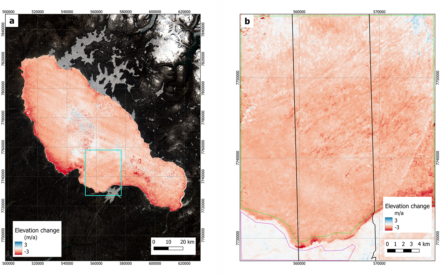
In addition to exploring frontal change, we also investigated changes in surface elevation via the ASTER dDEM product of Hugonnet (Reference Hugonnet2021). Figure 4 shows surface elevation change for the time period 2000–2020. Rates of change are shown in metres per year. Almost the entire region underwent surface lowering over the 20 year period, with only small regions at the summit of the ice cap exhibited thickening (Fig. 4).
Surface elevation change between 2000 and 2020 derived from the ASTER DEM-difference product (Hugonnet and others, Reference Hugonnet2021) at a resolution of 100 m. (A) The ASTER-derived elevation change over the entirety of the Barnes Ice Cap (turquoise box indicates the area shown in the right-most panel). The background is a Landsat 8 image from 28 July 2023. (B) Our area of interest (the central–southern outlet study region) as indicated in Figure 1, with the ArcticDEM strip-overlay section subsequently discussed marked in black. The green polygon marks the extent of the on-ice region investigated more in-depth. The pink polygon marks the equivalent off-ice region (see Figure 5).

To assess potential dDEM bias and errors, we monitor observed change over off-ice regions (pink polygon in Fig. 4b), which we assume should be stable over time, and compare it to ice surface elevation change over our study region (green polygon in Fig. 4b) over the 2000–2020 time period covered by the ASTER dDEM data (Fig. 5).
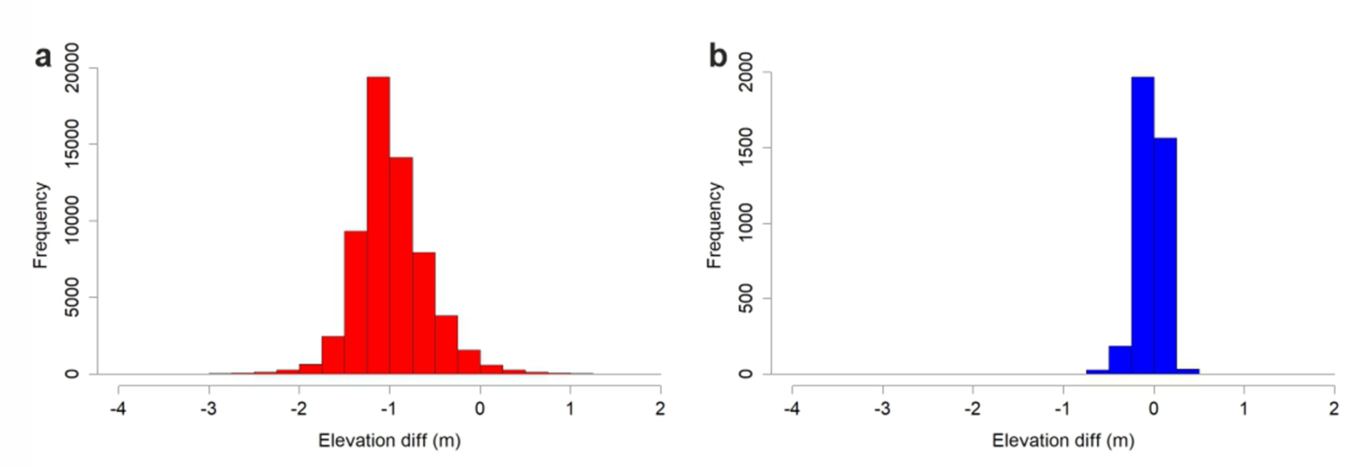
Histograms of surface elevation change between 2000 and 2020 derived from the ASTER DEM-difference product (Hugonnet, Reference Hugonnet2021) over on-ice (A) and off-ice (B) regions. The zones explored are highlighted in Figure 4. Over on-ice regions, the mean elevation change was −0.978 m a−1 and the median elevation change was −1.024 m a−1. Over off-ice areas the mean elevation change was −0.032 m a−1 and the median elevation change −0.018 m a−1.

The mean elevation change over the central-southern outlet study region of the Barnes Ice Cap was −0.978 m a−1 (a negative value means surface lowering) while the median elevation change was −1.024 m a−1. Over off-ice areas the mean elevation change was −0.032 m a−1 (median: −0.018 m a−1; Fig. 5). Consequently, the magnitude of change over the central-southern outlet study region is far greater than that observed over off-ice areas. We assume off-ice regions to be stable, albeit with the likely presence of small surface changes due to ice-cored moraines and unconsolidated surface material. The median value in this off-ice region (−0.018 ma−1) is substantially less than the standard deviation (0.130 ma−1) suggesting there is no significant systematic bias in our approach. Nevertheless, we take a conservative view that the changes observed in these off-ice areas indicate the minimum possible elevation change that can be confidently measured.
This on-ice rate of change for the central-southern outlet study region is very similar (but marginally less) than that for the entire Barnes Ice Cap (−1.062 ma−1). Hugonnet (Reference Hugonnet2021) report mean elevation change rates over the entire Arctic Canada South region (within which the Barnes Ice Cap is situated) of −0.77 ± 0.06 ma−1. The Barnes Ice Cap is therefore thinning at a rate faster than average for the Southern Canadian Arctic region. ITS_LIVE data also shows this central-southern outlet study region to be consistently the fastest moving part of the ice cap (Fig. 6).
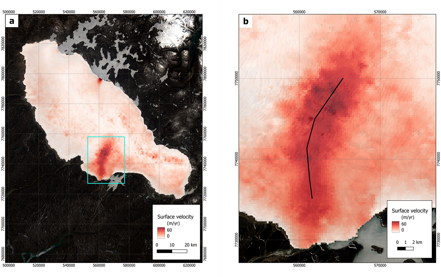
Surface velocities (ma−1) in 2018, derived from the ITS_LIVE platform (Gardner, Fahnestock, & Scambos, Reference Gardner, Fahnestock and Scambos2023). (A) Velocities over the whole of the Barnes Ice Cap, with the turquoise rectangle marking the central–southern outlet study region, which is the focus of (B). This shows velocities (using the same colour-scale) over the central–southern outlet study region. The black line represents an effective centreline along this fast-flow feature. The background image here is a Landsat 8 image from 28 July 2023, and channels visible in this image can be seen through the semi-transparent shading of surface velocities. The mean error across the whole of the Barnes Ice Cap is 0.86 ma−1; the mean error across the central–southern outlet study region is 0.96 ma−1.

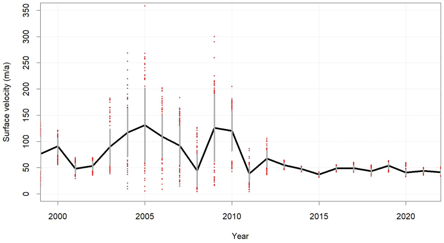
The mean ice velocity across the entirety off the Barnes Ice Cap is 9.55 m a−1 (standard deviation of 8.17 m a−1), whilst the mean velocity within our study area is 23.58 m a-1 (standard deviation of 13.91 m a−1) We also explored ITS_LIVE data over a number of time steps (1999–2022) and at multiple locations along a pseudo-centreline along the central-southern outlet study region. Over this time period, we not only observed a decreasing trend in surface velocity (Fig. 7) but also apparent changes in the variability of measurements. We attempt to explain the patterns of behaviour in the discussions.
Surface velocities (m a−1) at 162 separate points (in red) along an approximate centreline along the fast flow feature of the central–southern outlet study region. Points are located along the line marked in Figure 6b. The black line represents a mean velocity at all locations in each year while the grey vertical bars indicate the standard deviation in each year. The variation in velocity is particularly marked from 2003 to 2012, reducing substantially after 2012, while the feature appears to slow down from 2011 onwards.

4.2. Drainage networks from topographic data
4.2.1. Drainage network location and orientation
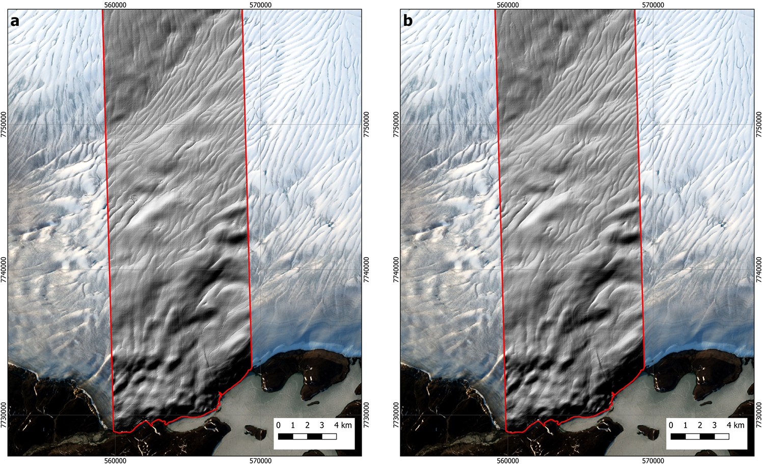
To explore the long-term evolution of supraglacial drainage pathways, we investigated ArcticDEM data in 2011 and 2020. Exaggerated hillshade models reveal a surface topography that is heavily dissected by a branching supraglacial channel network that is also visible in contemporaneous optical imagery (Fig. 8). Channels are clearly visible and close inspection of these two images reveals striking similarities, both in terms of larger-scale surface undulations and fine-scale linear features related to water flow.
Hillshaded DEM strips covering identical parts of the central–southern outlet study region: (A) 20 August 2011 and (B) 20 April 2020. Hillshades have been exaggerated by 15 times to enhance supraglacial topography associated with water channels. Note that these channels are also visible in the composite Landsat image in the background, which is a Landsat 8 image from 28 July 2023.

Following qualitative assessment, we quantitatively mapped channel distribution in the DEMs and display the resultant flow accumulation rasters as a polylines displaying the network of channels (Fig. 9).
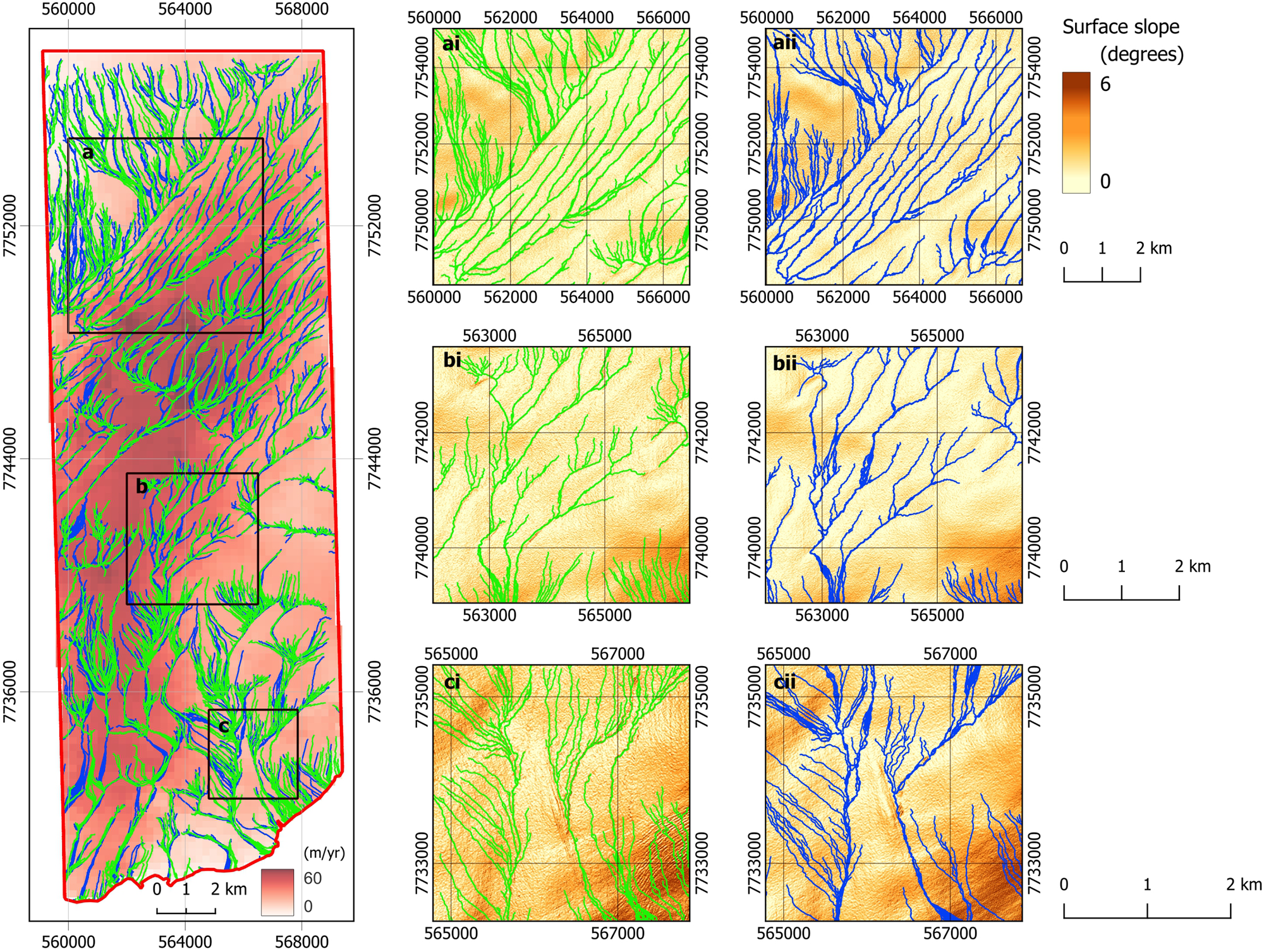
Drainage reconstructions based on DEM-derived channel locations on 20 August 2011 and 20 April 2020. The left-most panel shows drainage reconstructions from 2011 (green) and 2020 (blue) overlain onto the ITS_LIVE 2018 surface velocity mosaic (m a−1). Black boxes indicate the location of panels A, B and C. For panels, column (i) shows the reconstructed drainage pathways in 2011 (green), while (ii) shows the same in 2020 (blue). The background to panels (A–C) is the surface slope of the DEM from the respective years.

Superimposed channel networks from 2011 to 2020 showed remarkable similarity in drainage patterns between years (Fig. 9). Minor differences occur mainly in the lower-order channels. In some locations major drainage pathways are, to a large extent, found in the same place despite the nine-year time difference between strips. In some other locations, there appears to be a slight offset between the locations of these routeways, suggesting that these channels have been advected in the direction of ice flow.
In addition to the apparent persistence of channel locations, it is also interesting to note that the primary ice flow pathway, identified by a central region of higher velocities (darker reds in Fig. 9), appears to result in highly flow-aligned and parallel stream distributions. This is most clear in Figs. 9Ai and 9Aii where it seems that channels in the upper-left (north-west; NW) part of the image flow towards the centre of the image in a NW-SE orientation until they encounter the faster ice flow. On encountering this area of higher velocities, channel orientation abruptly changes to a NE-SW orientation, suggesting either that ice velocity has some role in stream orientation, or more likely that the controls on ice flow also control channel orientation. This pattern is replicated across the larger study region.
Channels are generally found on less steep terrain and steeper slopes are either unchanneled or display higher-order, less developed channel networks (Fig. 9). However, towards the ice margin where slopes become particularly steep, developed channels flow directly down the steep ice front.
4.2.2. Drainage channel persistence
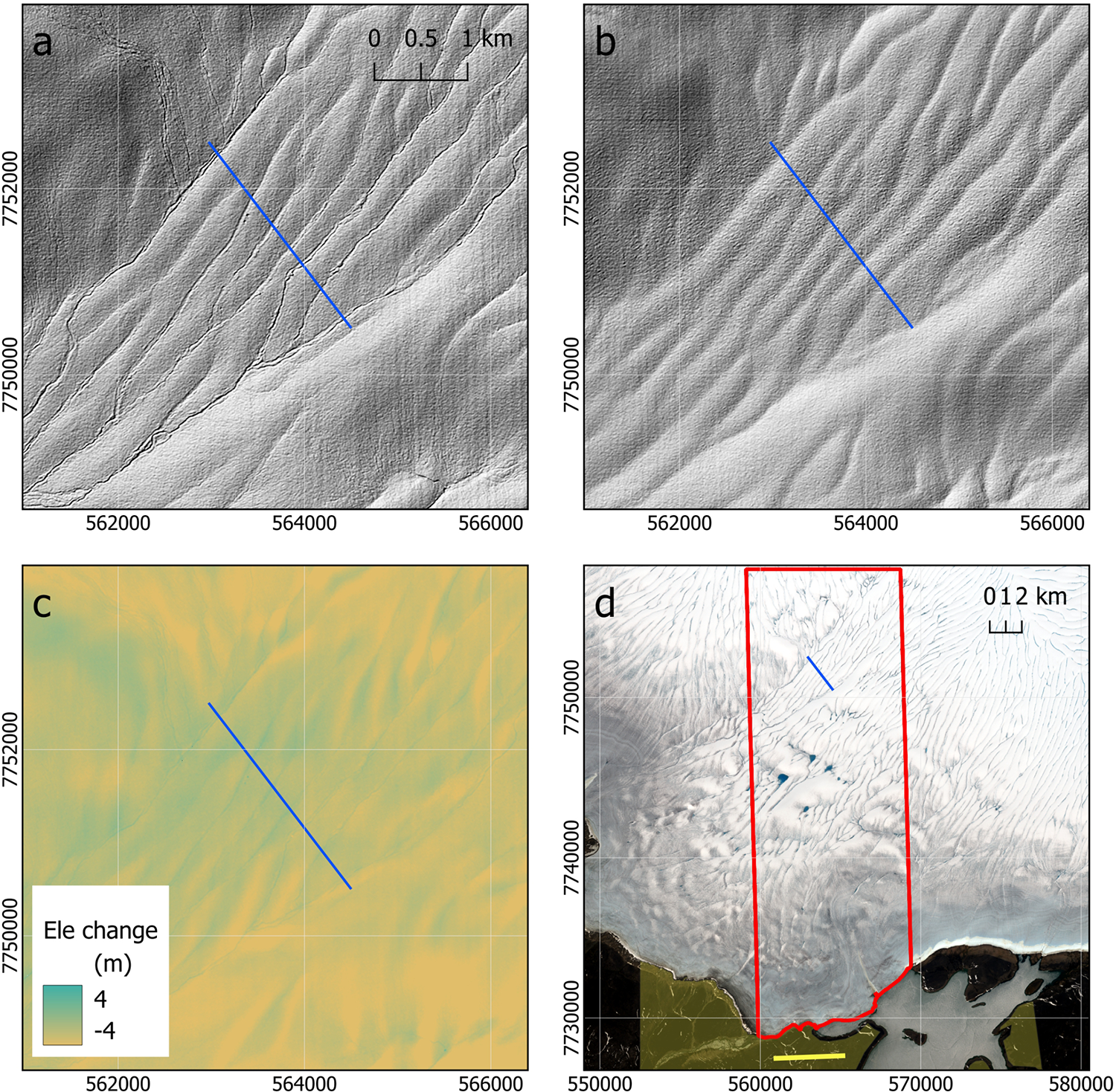
To explore changes in channel persistence in more depth, we take advantage of the high spatial and temporal resolution of ArcticDEM strip dataset. We identified 47 separate ArcticDEM stripfiles that at least partially overlap our wider region of study (Figs. 1 and 4). Within this, we delineated a short transect of ∼2.5 km (Fig. 10) which traversed a clear suite of supraglacial channels, identifying 28 strips (Table 3) that both overlap the transect and some of the forefield (off-glacier) area (necessary to co-register the stripfiles against stable bedrock).
The location of the 2.5 km long transect (blue line) where we explored high temporal resolution changes in surface shape. (A) ArcticDEM strips from 20 August 2011; (B) DEM from 20 April 2020; (C) the difference between the two DEMs; (D) larger regional view of the transect’s location, with the forefield (semi-transparent yellow) that was used as the off-glacier area for coregistration of the strip files, and an off-ice transect (yellow line) that is further explained in the text. The red polygon delineates the same area as in Figures 8 and 9.

Summary of ArcticDEM stripfiles available and used in this investigation. Files are listed by year, and it is notable that some years are much more readily served than others.

The dates in bold indicate where the stripfile overlaps both the cross-channel transect of interest and the off-ice co-registration area. The italicised dates are those where the stripfile covers the cross-channel transect but not the off-ice co-registration area. The bold dates with an asterisk are those that class as ‘summer’. Note that strips from 2 April 2019, 14 May 2019, 20 April 2020, 30 March 2021, 16 July 2021, 18 May 2022 and 7 June 2022 are coregistered to ICESat data.
Despite coregistration against stable bedrock, ArcticDEM strips do not necessarily display a secular lowering trend (Fig. 11). This is likely due to: (i) high intra-seasonal variability within the period which strips were captured (snowfall, surface melting, ice advection, dynamic processes and the role of flowing meltwater); and (ii) systematic elevation biases in the DEM strips (e.g. rotation and tilt) that are not corrected by our chosen coregistration approach (Nuth and Kääb, 2011), which only accounts for translation errors and is dependent on a coregistration reference site located distal to the transect of interest.
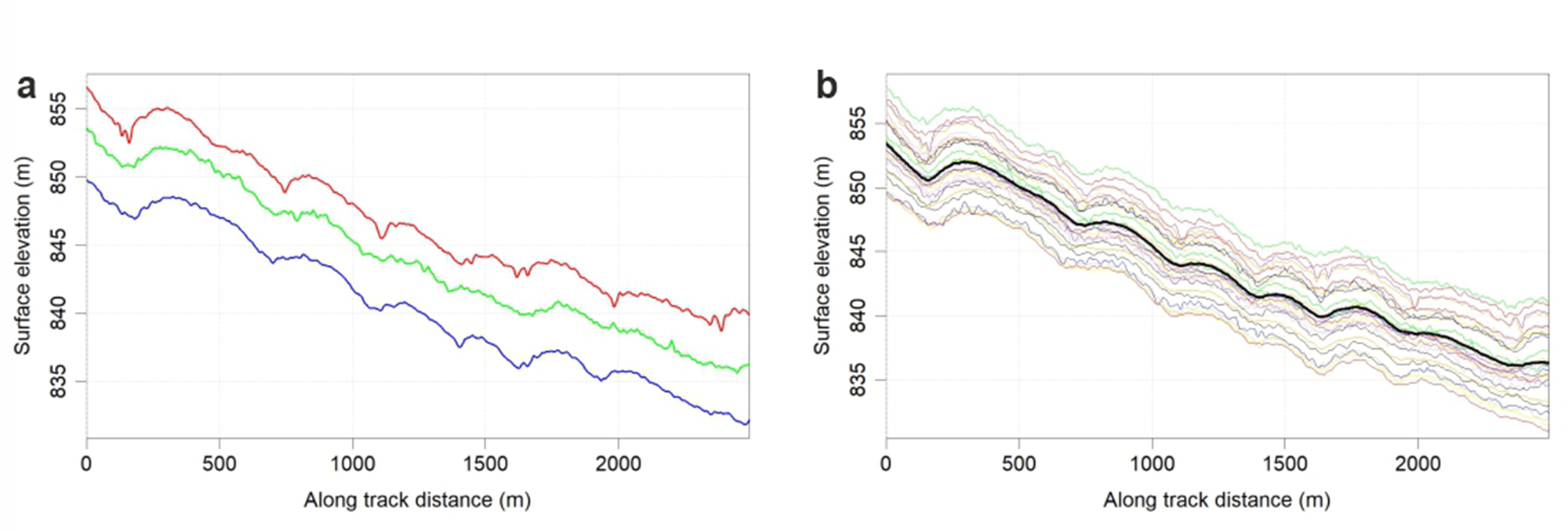
Surface profiles along the 2.5 km long transect shown in Figure 10 where the strip overlaps both the cross-channel transect of interest and the off-ice coregistration area. The plots run from the north-west to the south-east, and the seven channels seen in Figure 10 are clearly identifiable here. (A) Transects are shown for dates in July and August where to try to replicate the same time of year in each scenario—i.e. mid-to-late summer when snowcover should be at a minimum, and meltwater is flowing. The dates shown in this plot are 20 August 2011 (red); 1 July 2018 (green) and 16 July 2021 (blue). (B) Transects for all available stripfiles are shown so as to demonstrate the persistence of these channels across seasons and over the long term. Data here covers the period 6 April 2011 to 7 June 2022. The thick black line is the mean of all these 25 transects.

In order to minimise the effect of processes that might complicate such observations, we explore the surface at similar times of year, preferably at the end of the ablation season. The results of such an approach are shown in Fig. 11. The desire to explore change at a similar time each year means the vast majority of the stripfiles identified in Table 3 are not usable, and just three transects between 2011 and 2021 are shown. The dates of these transects are 20 August 2011, 1 July 2018 and 16 July 2021. There is consistent surface-wide lowering between 2011, 2018 and 2021 (Fig. 11).
The three summer transect indicate gradual surface lowering over the ∼10-year study period, as would be expected, at a mean annual rate of − 0.624 m a−1 between 2011 and 2021 (between 2011 and 2018 the rate is − 0.392 m a−1 while between 2018 and 2021 this accelerates to − 1.164 m a−1). Over the full time period, this derived magnitude of surface elevation change is somewhat lower than that derived from Hugonnet and others (Reference Hugonnet2021) and reported in Section 4.1.2, of −0.978 m a−1. However, the rate from ArcticDEM in more recent years exceeds the ASTER value. The discrepancy could indicate how rates of change are variable over shorter time periods but might also reflect the difficulties of using ArcticDEM strip data in such environments to identify change as we have mentioned here.
To assess the accuracy of the data, we looked at the difference in surface elevation in stripfiles over a transect of assumed stability in the off-ice area. As with the on-ice transects, we investigated change over a short period of time: 23–26 May 2012 and 14–28 April 2013. The mean difference in May 2012 was 0.020 m (mean magnitude difference of 0.051 m), while in April 2013, the mean difference was −0.006 m (mean magnitude difference of 0.014 m). Although these values are superficially small, expressed in the same units as above it becomes clear that substantial uncertainties exist, further calling into question the ability to use the ArcticDEM data to confidently quantify change in an ice surface.
Thus we find fundamental limitations in the ability to use the ArcticDEM stripfiles to explore short-term changes in ice elevation at the precision required for this study, given the highly dynamic environment, large distance from the ice margin and suboptimal coregistration conditions. What is striking, however, is the clear consistent presence of supraglacial channels as topographic lows in the terrain in approximately the same location over many years (Fig. 11a), that persist in all transects from these summer data. These channels are in fact visible in all transects from all the timesteps identified in Table 2 (Fig. 11b). This further demonstrates that such supraglacial channels are able to maintain their position over the long term.
4.3. Drainage networks from optical satellite imagery
The work presented in Section 4.2 demonstrates a surprising degree of stability in supraglacial channel location over a 9-year period, but we are interested to extend this analysis to investigate inter-annual persistence in channel locations over longer time periods using the longer Landsat record to explore channel evolution. To do this, we apply the approach of Rawlins and others (Reference Rawlins, Rippin, Sole, Livingstone and Yang2023) following Yang and others (Reference Yang, Smith, Chu, Gleason and Li2015) as outlined in the methodology (Fig. 12).
Mean surface drainage networks in 5-year time blocks, as determined through calculations of the NDWI in order to map out the presence of supraglacial water bodies. The 5-year time periods over which drainage was averaged are: (A) 1985–1989, (B) 1990–1994, (C) 1995–1999, (D) 2000–2004, (E) 2005–2009, (F) 2010–2014, (G) 2015–2019 and (H) 2020–2024. In each plot, an underlying composite Landsat 8 image from 28 July 2023 is shown, and lying on top of this (red-shading) is the ITS_LIVE 2018 ice surface velocity mosaic (m a−1). The blue lines show supraglacial water as identified in NDWI plots.

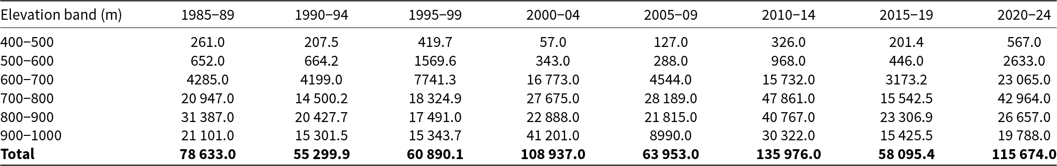
There is some evidence of an increase in the spatial extent of supraglacial drainage over the 49-year long record (Fig. 12). Total drainage extent between the first period (1985–1989) and the final period (2020–2024) does indeed increase, but over the intervening years there is some variability observed, with periods of greater drainage area (2000–2004 and 2010–2014) and periods of reduced drainage area (1990–1994 and 2015–2019). Similar patterns of behaviour are apparent when looking at discrete elevation bands too. This is summarised in Table 4.
Supraglacial drainage area over the time periods shown in Figure 12, by different elevation bands. Area is calculated from binary plots of drainage extent with the presence of water indicated by a value of 1 and no water a value of 0. The numbers in the table are therefore dimensionless (indicating the number of cells containing water over the study area) but could be converted to m2 by multiplying by the size of a Landsat cell (30 × 30m). Drainage area is indicated in 5-year time periods and is shown for different 100 m elevation bands and over the whole region.

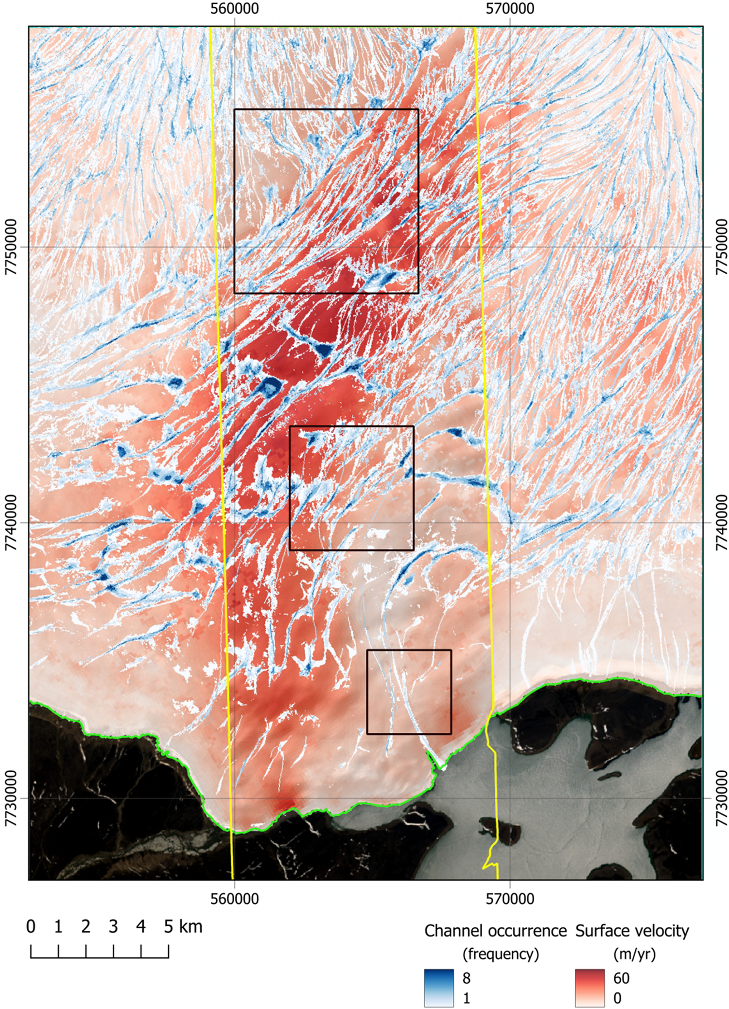
To highlight the regions of variability and overlap, we plot the accumulated incidence of water occurrence over all time periods (Fig. 13). Here, a darker blue thus indicate more frequent identification of a pixel as water across all Fig. 12 plots (and so reoccurrence as water). In this figure, we see that there are several major routeways that are reused in multiple time periods (darker blues) with an indication of more transient regions of drainage feeding into these. The image also highlights the occurrence of supraglacial lakes (larger areas of darker blue).
Per-pixel reoccurrence frequency of supraglacial drainage networks between 1985 and 2024, determined by summing all plots shown in Figure 12. Darker blue indicates more frequent reoccurrence. The background images are the same as in Figure 12. The yellow outline marks the ArcticDEM strip-overlay region discussed previously. The three black squares represent the areas of interest shown and discussed in Figures 9 and 14.

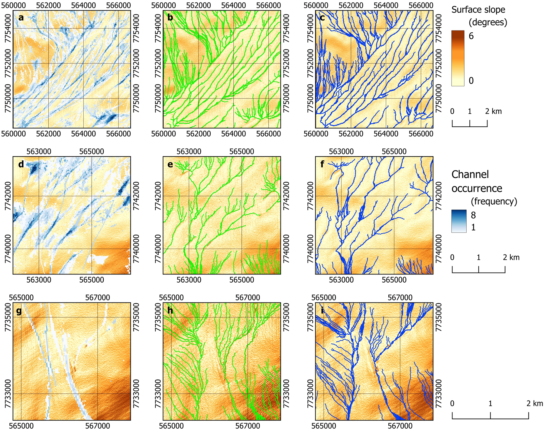
We further compare the NDWI Landsat-derived network with the DEM-derived network over contemporaneous time-steps (Fig. 14). The broad pattern revealed by both approaches of the higher-order (larger) channels is very similar, reinforcing the assertion that these drainage networks are indeed persistent over long periods of time. The NDWI product is less able to identify the smaller, lower-order channels, sometimes marking these are wider water-filled areas, or not indicating them as water-filled at all. This likely reflects the substantially lower resolution of these data.
Drainage networks in zoomed-in region A (top row), B (middle row) and C (bottom row) as defined in Figure 9, but also outlined in Figure 13. (A), (D) and (G) show cumulative supraglacial drainage networks between 1985 and 2024 derived from NDWI calculations (see Figures 12 and 13 for more details). (B), (C), (E), (F), (H) and (I) are identical to those plots shown in Figure 9, but are reproduced here for ease of comparison with the NDWI plots. These are reconstructed drainage pathways based on the ArcticDEM strip from 2011 and 2020. The background to all images is the surface slope.

5. Discussions
Our overarching purpose in this paper was to explore how drainage networks on the Barnes Ice Cap have evolved over time. In order to achieve this, and in recognition of the fact that it is water generated by melt from the ice cap surface that drives the discharge in these streams, we initially focussed on changes in the overall size of the ice cap, as driven by contemporary warming patterns. We then investigated in-depth, how supraglacial hydrological drainage networks vary temporally and spatially.
5.1. Geometrical changes
Our investigations reveal retreat of the ice margin and lowering of the surface (derived from analyses of Landsat imagery and the ASTER dDEM products, respectively). Our focus was on the fastest-flowing region of the Barnes Ice Cap over the 40-year period of our investigation (1983–2023), which showed a mean total retreat of 158.14 m (averaging 3.95 m a−1).
The ASTER dDEM product further enabled us to explore surface elevation change over just 20 years (2000–2020). The mean rate of change in the central–southern outlet study region was −0.978 m a−1, peaking at −1.76 m a−1. This thinning rate was similar but marginally greater than that for the entire Barnes Ice Cap of −1.062 m a−1. Hugonnet and others (Reference Hugonnet2021) report mean elevation change rates between 2000 and 2019 over the entire Arctic Canada South region (within which the Barnes Ice Cap is situated) of −0.77 ± 0.06 m a−1. The Barnes Ice Cap as a whole, and parts of the central–southern outlet study region are therefore thinning at a rate somewhat higher than that observed over the Southern Canadian Arctic. There are very small regions of apparent minimal thickening (largely outside of our study area, at the highest parts of the ice cap); perhaps as a result of the predicted increased precipitation that accompanies atmospheric warming (Tabari, Reference Tabari2020; Zhang and others, Reference Zhang2024). However, these regions constitute only a very small part of the wider ice cap (1.061%).
The elevated thinning rates in our study area are not entirely surprising since according to ITS_LIVE data, this is the fastest moving part of the ice cap by some way (Fig. 6). The mean ice velocity across the entirety off the Barnes Ice Cap in 2018 is 9.55 m a−1, but the mean velocity within our study area is more than twice this at 23.58 m a−1, peaking in some areas at 62.52 m a−1. Nevertheless, despite this being the fastest flowing part of the ice cap, our investigations suggest that this region has perhaps slowed down over the past 23 years. However, we are reluctant to rely too much on this observation since more prominently in Fig. 7 is a decrease in variability of velocity measurements after ∼2012. In fact, closer observation reveals that variability in measurements increases markedly after 2002 and persists until 2012. This period coincides with the beginning of the SLC-off period associated with Landsat 7 (Wang and others, Reference Wang, Wang, Wei, Jin, Li, Tong and Atkinson2021). We are thus reluctant to over-interpret this apparent slowdown. If we treat velocities in this period with caution, then annual surface velocities appear to have been remarkably consistent at this higher level, with little difference in mean surface velocity between the pre-2003 period and the post-2012 period. As a result, dynamic thinning (whereby thinning occurs because of increasingly fast drainage of ice (Shuman and others, Reference Shuman, Berthier and Scambos2011; Flament and Rémy, Reference Flament and Rémy2012)) might have a less important role in the observed ice thinning. Under such a scenario, where there is no significant change in ice velocity yet mass balance remains consistently negative and surface lowering continues, melt-driven surface lowering must play an important role.
The observed mass loss at the Barnes Ice Cap coupled with the rapid (but consistent) ice flow rates is significant and thus it is clear that the Barnes Ice Cap and particularly our study area deserves significant attention. If melt-driven lowering is so important, then characterising the generation and movement of this meltwater is key. We therefore subsequently focus on the nature and variability of drainage.
5.2. Surface hydrology
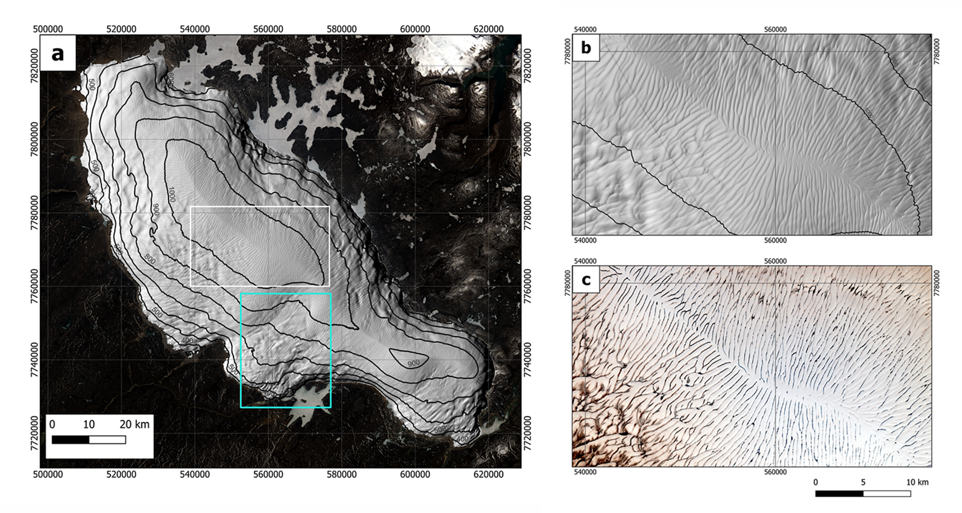
ArcticDEM data reveal an extremely detailed surface topography that is dominated at 10-100 m scales by a complex network of supraglacial channels carved into the ice surface. The surface of the Barnes Ice Cap is heavily dissected by supraglacial channels, and, within the limitations of the 2 m DEM resolution, they appear to be up to several tens of metres across, and several metres deep. They are visible in both ArcticDEM and Landsat data (Fig. 15) over nearly the entire ice cap, extending from virtually the highest point of the ice cap (at an elevation of ∼1097 m) to the margins in all directions.
(A) 2 m ArcticDEM mosaic (v4.1, made of amalgamated datasets from ∼2007 to the present) of the Barnes Ice Cap (Porter and others, Reference Porter2023), displayed as grey-scale representations of hillshaded topography exaggerated by 15 times, with 100 m surface elevation contours shown. The turquoise rectangle marks the central-southern outlet study region. The white rectangle highlights a region of the central, highest part of the Barnes Ice Cap, which is shown in panels (B and C). (B) The same hillshaded DEM whilst part (C) shows a Landsat 8 image form 28 July 2023. In (A), it is apparent that drainage channels cover virtually the whole of the Barnes Ice Cap. (B and C) This coverage extends all the way up to the ice divide at an elevation of ∼1097 m. Displaying both the DEM and a Landsat image serves to demonstrate that not only are channels present (ArcticDEM) but that they also visibly carry water and thus are active.

In carrying out this work, we expected to see an evolution of supraglacial drainage similar to that observed in Greenland—i.e. that as a result of increasing atmospheric temperatures the amount of melting would also increase, leading to an expansion of the drainage system reaching to increasingly high elevations as temperatures and melting increased (Smith and others, Reference Smith2015; Gleason and others, Reference Gleason2016, Reference Gleason2021; Pitcher and Smith, Reference Pitcher and Smith2019; Yang and others, Reference Yang2021; Rawlins and others, Reference Rawlins, Rippin, Sole, Livingstone and Yang2023). The main outcomes of our study, however, are somewhat different. As shown in Section 5.1, increasing mass loss by surface lowering did occur. However, over the 9-year period covered by the ArcticDEM analysis, we observe minimal variation in drainage routing. As reported in Section 4.2.1, there are some minor differences (mainly in the lower-order channels), but overridingly, the major drainage pathways are essentially the same between these two dates. Over the longer Landsat observational period (49-year from 1985 to 2024), we once again observed that despite some variability in the smaller lower-order channels, those of a higher order are remarkably persistent, and match well with those seen in the higher-resolution ArcticDEM investigations (Fig. 14). In addition, although there is perhaps some evidence of an increase in the spatial extent of supraglacial drainage over the 49-year long record (Fig. 12), for the most part we see that elevation-wise, the drainage has not expanded since the channels/drainage have already existed at the lowest-highest elevations across the time period. This is different to the situation occurring in Greenland where channels expand inland. This cannot happen on the Barnes Ice Cap as channels here already reach those highest elevations.
Over multi-annual time periods, the topographic form of the supraglacial environment is primarily driven by two processes. Firstly, ablation (or accumulation), which serves to lower (or raise) the ice surface (Ryan and others, Reference Ryan2019; Irvine-Fynn and others, Reference Irvine-Fynn2022). Despite some variability, the ice surface across the central–southern outlet study region (and much of the Barnes Ice Cap itself) shows significant surface lowering over time, indicative of substantial mass loss (Fig. 4). Rates of surface lowering vary in response to differing inputs of energy (moderated by variations in surface albedo, aspect, slope, etc.), but nevertheless, widespread surface ablation acts to smooth the surface and remove surface roughness obstacles.
The second process controlling the topographic form of the ice surface is the thermo-mechanical incision of flowing meltwater. While we envisage that widespread surface lowering by ablation generally serves to smooth an ice surface, the significant erosive power of cold, fast-flowing water on a highly erodible ice surface, and the fact that such channels are spatially discrete, increases surface roughness through the cutting of channels (Rippin and others, Reference Rippin, Pomfret and King2015; Irvine-Fynn and others, Reference Irvine-Fynn2022).
The marked surface lowering observed and reported here, alongside the persistent supraglacial drainage network suggests that despite widespread surface lowering through ablation, erosion by flowing water is of such a magnitude as to ensure that the drainage pathways persist year after year. Such significant and widespread surface ablation means that we might expect a drainage network that evolves substantially over the course of a melt season, with new channels easily being created as increasing volumes of water are generated. Similarly, we might expect similar evolution between melt seasons too (Irvine-Fynn and others, Reference Irvine-Fynn, Hodson, Moorman, Vatne and Hubbard2011; Lampkin and Vanderberg, Reference Lampkin and Vanderberg2014; Lu and others, Reference Lu2020). The fact that there is no such evolution, and that the channels show remarkable persistence year after year is counter to expectations, yet it implies that meltwater-forced erosion is greater than atmospheric mass loss, and so channels will incise more quickly than melting can flatten out a surface. If the channels remain constant then the incision rate must have to be constant in a steady state system, or if mass balance is increasingly negative, correlate with the increasing availability of meltwater. Further research into this topic would be of significant interest. However, it is important to note that there may well be channels smaller than the resolution resolvable which are more transient.
5.3. Controls on channel location
While we suggest that persistent supraglacial channels dominate on the Barnes Ice Cap, it is important to determine whether stream channels persist for lengthy periods of time being reused each year, or whether they repeatedly re-form in the same location each year due to some broader, underlying control. Through an analysis of all the ArcticDEM stripfiles over the entire ablation season (and beyond) of 2016 (Table 3), we see that the channels are evident and persistent from March to November 2016. It is thus clear that these channels likely do not reform each year, but rather they persist. Over much of the region of interest, both surface slope and ice velocity appear to have a controlling influence on channel location and orientation, with streams generally being found on less steep terrain with a trend for channels to orientate in the direction of ice flow (Lu and others, Reference Lu2021). Together, this suggests that the ice thickness and thus underlying basal topography have a control on channel location.
The concept of a role for bed topography in controlling channel location is akin to studies of supraglacial lakes on Greenland. These have been observed to remain in essentially the same location due to control exerted by the underlying bed topography. As has been discussed by Ignéczi and others (Reference Ignéczi2016, Reference Ignéczi, Sole, Livingstone, Ng and Yang2018), surface topography reflects underlying bed topography (albeit damped over scales of ice thicknesses), and so depressions or valleys in the bed manifest as such on the ice surface. Ignéczi and others (Reference Ignéczi, Sole, Livingstone, Ng and Yang2018) state that although large-scale drainage structure is controlled by surface topography, which is in turn controlled by basal topography, this is only at length scales comparable to the ice thickness. Consequently, it is unlikely that bed topography exerts an influence on the location of individual, discrete drainage pathways. However, ice velocity and surface slope are both controlled by underlying topography and our investigations indicate a close relationship between these two parameters and channel location. To explore the role of basal topography more fully, we explored this in our zone of interest.
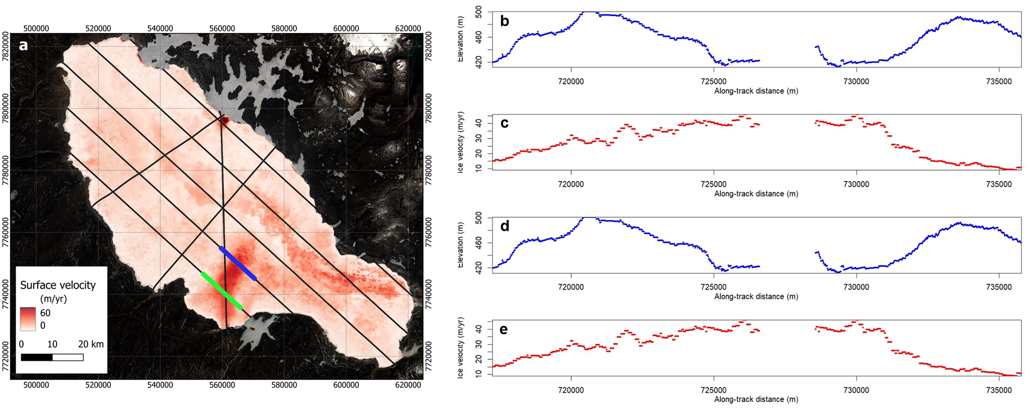
There are limited data available concerning the topography beneath the Barnes Ice Cap, but NASA’s ‘Operation IceBridge’ collected several lines of radio echo-sounding data, albeit sparse, over the Barnes Ice Cap in 2011 (Fig. 16; https://nsidc.org/data/icebridge/data; Paden and others, Reference Paden, Li, Leuschen, Rodriguez-Morales and Hale2019). Unsurprisingly, the fast-flow feature studied here appears to lie in a bedrock trough, and so there is clear topographic control on ice dynamic behaviour in the region. However, drainage pathways exist across the entirety of the Barnes Ice Cap, regardless of whether the bed topography is deep or shallow (Fig. 15), suggesting this is not a control on channel incidence.
(A) Location of Operation IceBridge RES survey lines gathered in May 2011. The black lines show the extent of all RES surveys, while the blue and green sections highlight transects that cross the fast-flow region in our area of interest. The red-shading represents ITS_LIVE 2018 surface velocity mosaic (m a−1). Line graphs represent the bed elevation (B) and surface velocities (C) along the upper transect marked in blue in the left-hand panel. (D and E) represent the same but for the transect marked in green. The background image here is a Landsat 8 image from 28 July 2023.

To summarise, bed topography no doubt exerts an influence on the broad shape of the ice surface, and on ice dynamics. Through this, there is some influence on drainage network behaviour, but not on individual channels. Individual channels are most likely initially initiated by subtle variations in surface roughness, which is in part influenced by the channels themselves. Once established, the channels appear to be reused year after year, exhibiting extraordinary stability. We also note that at the resolution of the imagery explored, the vast majority of channels appear to persist all the way to the ice margin, and thus there is a distinct lack of interruption of channels by crevasses or moulins in our area of interest. As a result, despite the large amount of water that we believe is channelled through this network, we tentatively suggest that little of this reaches subglacial locations, with most of it travelling supraglacially.
Rippin and others (Reference Rippin, Pomfret and King2015) identified the existence of a series of deeply-incised supraglacial channels on the surface of the polythermal glacier Midtre Lovénbreen in Svalbard that are reused year after year (cf. Irvine-Fynn, Reference Irvine-Fynn, Hodson, Moorman, Vatne and Hubbard2011; Karlstrom and others, Reference Karlstrom, Gajja and Manga2013), as well as a more temporary and widespread network of smaller channels that is reinstated each year. This is in contrast to channel migration observed by Irvinne-Fynn and others (Reference Irvine-Fynn2022) and indeed the typical way in which hydrology is believed to evolve on an ablating glacier (Hambrey, Reference Hambrey1977; Irvinne-Fynn and others, Reference Irvine-Fynn2022). We suggest that where atmospheric ablation is higher than channel incision, incised channels are preferentially removed, whereas in our scenario the reverse is the case and channels persist (e.g. Marston, Reference Marston1983; Pitcher and Smith, Reference Pitcher and Smith2019; Wytiahlowsky and others, Reference Wytiahlowsky, Stokes, Hodge, Clason and Jamieson2025).
In general, supraglacial drainage evolution over timescale of any substantial duration has been ignored or overlooked to date. Perhaps the most substantial observation derived from our investigation is to reveal the presence of not only extensive and repeatedly reused channels on multi-annual timescales, but on longer, multi-decadal timescales too. These channels are important because they provide highly efficient routes for meltwater to exit the ice cap, impacting the ease with which mass is lost. Consequently, not only is there significant melting, but this is rapidly transited across the ice cap and removed from the system, thus constituting mass loss. Further research on this topic should focus on exploring the balance between atmospheric ablation and channel incision and how this impacts channel persistence and speed of meltwater evacuation. It should also focus on exploring the controlling mechanisms that lead to persistent channels occurring and indeed what circumstances are required by scenarios where large interannual variation can occur.
6. Conclusion
The Barnes Ice Cap as a whole has experienced negative mass balance since the end of the 19th century, with an increasing rate of negative mass balance since the mid-1990s (Abdalati and others, Reference Abdalati2004; Sneed and others, 2008; Gardner and others, Reference Gardner, Moholdt, Arendt and Wouters2012; Gilbert and others, Reference Gilbert2016, Reference Gilbert, Flowers, Miller, Refsnider, Young and Radić2017). In line with this increasingly negative mass balance, we explored how the meltwater that is a product of this mass loss is transferred across the ice cap, by exploring how supraglacial drainage has changed and evolved over the 39 years between 1985 and 2024, given the potentially key role that such drainage expansion might have for subsequent ice-mass loss. Our hypothesis was that an increasing and expanding drainage network would exist, driven by these mass balance changes. Surprisingly, however, rather than an expansion of the drainage network, from 1987 onwards, there was a remarkable persistence in drainage network location, orientation and density at ∼10–100 m scales—finer than that which would be imposed by subglacial topography. These supraglacial drainage pathways are clearly visible in both Landsat imagery and ArcticDEM stripfiles and display high interannual and decadal stability. Furthermore, they are present everywhere apart from the summit ridge of the ice cap, acting as a drainage divide. Unlike Greenland therefore, there appears to be minimal large-scale evolution of drainage to higher elevations and, instead, substantial ice cap-wide persistence of such unusually stable supraglacial drainage up to its drainage divide is surprising.
The presence of such persistent channels has two main implications. Firstly, it suggests that meltwater generated anywhere on the Barnes Ice Cap is presumably relatively easily transited to these channels, meaning it is evacuated rapidly and efficiently from the ice cap once the melt season starts. Secondly, we hypothesise that the re-use of channels each year means that they are deeply cut several metres into the ice surface and outpaces annual ablation rates. Gulley and others (Reference Gulley, Benn, Mueller and Luckman2009; cf. Chandler and Hubbard, Reference Chandler and Hubbard2023) discussed how persistent supraglacial channels may become englacial, through a process known as cut-and-closure. In extreme cases, these channels can become subglacial, where basal sliding can be affected through changes in water pressure distribution, which may result in more complicated changes in ice dynamics and mass loss. Although we do not observe directly that this is or is not happening on the Barnes Ice Cap, it seems likely that extensive, persistent and deeply incised supraglacial channels have the potential to evolve in this way.
Acknowledgements
We thank the two reviewers and Scientific Editor, Rachel Carr, for their thoughtful and helpful insights into our paper.
Data availability
ArcticDEM strips are provided by the Polar Geospatial Center (https://www.pgc.umn.edu/data/arcticdem/) under NSF-OPP awards 1043681, 1559691, 1542736, 1810976 and 2129685. We acknowledge the US Geological Survey for use of Landsat 4, 5, 7 and 8 from 1983 to 2023 (Earth Resources Observation and Science (EROS) Center, 2020a, 2020b, 2020c). These Landsat data are available from the US Geological Survey (https://earthexplorer.usgs.gov/). Velocity data was generated using auto-RIFT and provided by the NASA MEaSUREs ITS_LIVE project (https://its-live.jpl.nasa.gov/). We also acknowledge NASA’s Operation IceBridge (https://nsidc.org/data/icebridge/data) for some data used in this study. All other data are available on request.


 Open access