2.1. Axisymmetric governing equations

We consider a free-surface layer of conducting fluid of depth $h$ in the annular gap between two cylindrical electrodes of radius $r_i$ and $r_o$ ($r_i< r_o$). A controlled current $I$ runs through the fluid from inner to outer electrode, and the entire annulus is subject to a vertical, imposed magnetic field $\boldsymbol {B} = -B_0 \boldsymbol {e_z}$. Figure 1(a) shows a schematic of the annular channel with the imposed magnetic field and current. For a low-conductivity fluid like saltwater and small $B_0$, the magnetic field is quasi-static (e.g. Knaepen & Moreau Reference Knaepen and Moreau2008; Favier et al. Reference Favier, Godeferd, Cambon, Delache and Bos2011; Davidson Reference Davidson2016; Verma Reference Verma2017) and the total Lorentz force on the fluid may be expressed as the sum of the applied driving force and magnetic drag,

(2.1)\begin{equation} \boldsymbol{F}=\boldsymbol{J}\times\boldsymbol{B}=\sigma(\boldsymbol{E}\times\boldsymbol{B}) - \sigma B_0^2(u_r \boldsymbol{e}_r + u_\theta \boldsymbol{e}_\theta), \end{equation}

after using Ohm's law to express the current density $\boldsymbol {J}$ in terms of the electrical conductivity of the fluid $\sigma$, the imposed electric field $\boldsymbol {E}$ and the fluid velocity $\boldsymbol {u}$.

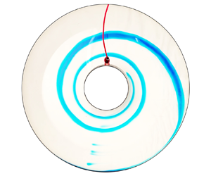
Figure 1. (a) Diagram of the magneto-Stokes system. A power supply controls the electric current $I$ through the fluid layer. Radially outwards ($+\boldsymbol {e}_r$) current density $\boldsymbol {J}$ and downwards ($-\boldsymbol {e}_z$) magnetic field $\boldsymbol {B}$ produce an azimuthal ($+\boldsymbol {e}_\theta$) Lorentz force $\boldsymbol {F}$ on the fluid. (b) Photograph of the channel used in laboratory experiments, with flow visualised by blue dye. The channel rests atop a wooden case of permanent magnets, which is replaced by a solenoid electromagnet (not pictured) for cases I–IV discussed in § 3.

Letting $U$ denote a characteristic velocity scale, the magnitude of the magnetic drag (${\sim }\sigma B_0^2U$) may be compared with that of the viscous drag (${\sim }\varrho \nu U/h^2$) by means of the Hartmann number,

(2.2)\begin{equation} {Ha} = \sqrt{\frac{\sigma B_0^2U}{\varrho\nu U/h^2}} = B_0 h\sqrt{\frac{\sigma}{\varrho\nu}}, \end{equation}

where $\varrho$ and $\nu$ are the density and kinematic viscosity of the fluid, respectively.

In our experiments, ${Ha} \lesssim 10^{-2}$ and thus the only component of current density $\boldsymbol {J}$ that makes a significant contribution to the Lorentz force is $\sigma \boldsymbol {E}$, which may be determined purely from the electric boundary conditions. A DC power supply can control the voltage across the sidewalls such that the total current $I$ is set to a desired value at each time $t$. In this case, current rather than voltage is used as a control parameter, and the Lorentz force is appropriately expressed as

(2.3)\begin{equation} \boldsymbol{F} = \sigma(\boldsymbol{E}\times\boldsymbol{B})= \frac{B_0 I(t)}{2 {\rm \pi}r h}\boldsymbol{e_\theta}, \end{equation}

neglecting any fringing of electric field lines due to the finite fluid depth (i.e. assuming that $\partial _z \boldsymbol {E} = 0$).

The resulting circulatory flow is governed by the incompressible equations of motion,

(2.4a,b)\begin{equation} \partial_t \boldsymbol{u} + \boldsymbol{u}\boldsymbol{\cdot}\boldsymbol{\nabla}\boldsymbol{u} ={-}\frac{1}{\varrho}\boldsymbol{\nabla} p + \nu \nabla^2 \boldsymbol{u}+ \frac{1}{\varrho}\boldsymbol{F},\quad \boldsymbol{\nabla}\boldsymbol{\cdot}\boldsymbol{u} = 0, \end{equation}

where $p$ is the deviation in pressure from the static pressure field $\varrho g (h-z)$.

We scale radial distances $r$ by the outer sidewall radius $r_o$, vertical distances $z$ by the fluid depth $h$ and electric current $I$ by its maximum value $I_0$, defining the non-dimensional quantities $\rho = r/r_o$, $\zeta =z/h$ and $\varUpsilon = I/I_0$. A velocity scale $U$ may be found by balancing the basal viscous drag (${\sim }2{\nu U}/{h^2}$) and Lorentz forces (${\sim }B_0 I_0/[{\rm \pi} h \varrho (r_i+r_o)]$) at the surface mid-gap, $z=h$, $r=(r_i+r_o)/2$:

(2.5)\begin{equation} U = \frac{B_0 I_0 h}{2 {\rm \pi}\nu \varrho (r_i+r_o)}. \end{equation}

This scale is used to produce the non-dimensional velocity $\boldsymbol {\upsilon } = \upsilon _\rho \boldsymbol {e_r} + \upsilon _\theta \boldsymbol {e_\theta } + (h/r_o)\upsilon _\zeta \boldsymbol {e_z}$, with components $\upsilon _\rho = u_r/U$, $\upsilon _\theta = u_\theta /U$ and $\upsilon _\zeta = (r_o/h) u_z/U$. An inertial scale $\varrho {U}^2$ is used to non-dimensionalise reduced pressure as $\varPi = p/(\varrho {U}^2)$. Time is non-dimensionalised as $\tau = t/T$ by a surface mid-gap advective time scale:

(2.6)\begin{equation} T=\frac{r_i+r_o}{U}. \end{equation}

In sum, our non-dimensionalisation makes the mapping

(2.7)\begin{equation} (\boldsymbol{u}, p, I)(r,\theta,z,t) \mapsto (\boldsymbol{\upsilon}, \varPi, \varUpsilon)(\rho,\theta,\zeta,\tau). \end{equation}

We introduce an a priori control Reynolds number $Re$ and a magnetic Reynolds number ${Rm}$,

(2.8a,b)\begin{equation} Re = \frac{h^2/\nu}{T} = \frac{B_0 I_0 h^3}{2 {\rm \pi}\nu ^2 \varrho (r_i+r_o)^2} \quad \text{and} \quad {Rm} = \frac{h^2/\eta}{T} = \frac{\nu}{\eta}Re, \end{equation}

where $\eta = (\mu _0 \sigma )^{-1}$ is the fluid's magnetic diffusivity and $\mu _0$ is the magnetic permeability of free space. For ${Rm} \ll 1$, magnetic diffusion dominates over advection, and the quasi-static description of the Lorentz force (2.3) is valid (e.g. Knaepen & Moreau Reference Knaepen and Moreau2008; Favier et al. Reference Favier, Godeferd, Cambon, Delache and Bos2011; Davidson Reference Davidson2016; Verma Reference Verma2017). As defined, ${Rm} \lesssim 10^{-10}$ for our experiments.

Also relevant are the radius ratio $\mathcal {R}$, aspect ratio $\mathcal {H}$ and depth-to-gap-width ratio $\varGamma$:

(2.9a–c)\begin{equation} \mathcal{R} = r_i/r_o, \quad \mathcal{H} = h/r_o, \quad \text{and} \quad \varGamma = h/(r_o-r_i) = \mathcal{H}/(1-\mathcal{R}). \end{equation}

Symbols for all dimensional parameters are listed in table 1. Definitions of scales and non-dimensional parameters are collected in table 2. The full non-dimensional axisymmetric equations in scaled cylindrical coordinates ($\rho,\theta,\zeta$) may be found in Appendix A.

Table 1. Dimensional parameter definitions. Values are given in § 3.

Table 2. Scales and non-dimensional parameters. All quantities below the dashed line are non-dimensional.

We assume vertical hydrostasy, $0={\partial _{\zeta }\varPi }$, and cyclostrophic balance, ${\upsilon _{\theta }^2}/{\rho }=\partial _{\rho }\varPi$, achieved via deflection of the free surface. Under these conditions, the meridional flow $\boldsymbol {\upsilon }_\bot = \upsilon _\rho \boldsymbol {e_r} + \mathcal {H}\upsilon _\zeta \boldsymbol {e_z}$ vanishes, leaving a linear equation for azimuthal magneto-Stokes flow,

(2.10)\begin{equation} Re\, \partial_{\tau}\upsilon_{\theta }={\nabla}^{2}_{\bot} \upsilon_\theta - \mathcal{H}^2\frac{\upsilon_\theta}{\rho^2} +\frac{\mathcal{R} +1}{\rho}\varUpsilon(\tau), \end{equation}

where we have defined the operator

(2.11)\begin{equation} {\nabla}^{2}_{\bot}({\cdot}) = \left[\mathcal{H}^2 {\rho}^{{-}1} \partial_{\rho}{\rho}\partial_{\rho} + \partial_{\zeta}^2\right] ({\cdot}). \end{equation}

We consider the rectangular domain $(\rho,\zeta ) \in (\mathcal {R},1)\times (0,1)$ with boundary conditions

(2.12)\begin{equation} \upsilon_\theta(\mathcal{R},\zeta,\tau)=\upsilon_\theta(1,\zeta,\tau)=\upsilon_\theta(\rho,0,\tau) = \left[\partial_{\zeta} \upsilon_\theta\right]_{\zeta=1} = 0. \end{equation}

This approximation to the free-surface boundary conditions is appropriate as long as the deflection due to capillary action and centrifugation is negligible (e.g. Greenspan & Howard Reference Greenspan and Howard1963). The Froude number ${Fr}$ compares the deflection of the free surface due to centrifugation (${\sim }U^2 g^{-1}$) with the depth of the fluid ($h$):

(2.13)\begin{equation} {Fr} = \sqrt{{U^2 g^{{-}1}}/{h}}. \end{equation}

Surface deflection due to capillary rise or dewetting is characterised by the capillary length (e.g. Martino et al. Reference Martino, De La Mora, Yoshida, Saito and Wilkes2006), $l = \sqrt {\gamma /(\varrho g)}$. The Bond number ${Bo}$ compares this length scale with the fluid depth:

(2.14)\begin{equation} {Bo} = (h/l)^2 = \varrho g h^2/\gamma. \end{equation}

In our validation experiments, ${Fr} \lesssim 10^{-2}$ and ${Bo} \geqslant 4.4$, so we adopt (2.12).

2.2. Spin up from rest

Solutions to (2.10), (2.12) that develop from an initially quiescent fluid ($\upsilon _\theta =0$ at $\tau = 0$) once constant electric current is applied ($\varUpsilon = 1$ for $\tau >0$) may be expressed as

(2.15)\begin{equation} \upsilon_\theta(\rho,\zeta,\tau) = \bar{\upsilon}_\theta(\rho,\zeta) + \upsilon_\theta'(\rho,\zeta,\tau). \end{equation}

The stationary component is

(2.16)\begin{align} \bar{\upsilon}_{\theta}(\rho,\zeta)&=\left(\frac{\mathcal{R}+1}{2}\right)\frac{2\zeta-\zeta^2}{\rho}\nonumber\\ &\quad -\sum_{n=1}^{\infty}\frac{2(\mathcal{R}+1)}{k_n^2 \mathcal{H}} \left[A_n {\rm{I}}_1\left(\frac{k_n }{\mathcal{H}}\rho\right)+B_n {\rm{K}}_1\left(\frac{k_n }{\mathcal{H} }\rho\right)\right] \sin (k_n \zeta), \end{align}

with

(2.17a)$$\begin{gather} A_n=\frac{\mathcal{H}}{k_n \mathcal{R}}\left[\frac{\mathcal{R} {\rm{K}}_1\left({k_n \mathcal{R}}/{\mathcal{H} }\right)-{\rm{K}}_1\left({k_n }/{\mathcal{H}}\right)}{{\rm{I}}_1\left({k_n}/{\mathcal{H} }\right) {\rm{K}}_1\left({k_n\mathcal{R} }/{\mathcal{H}}\right)-{\rm{K}}_1\left({k_n}/{\mathcal{H} }\right) {\rm{I}}_1\left({k_n \mathcal{R} }/{\mathcal{H}}\right)}\right], \end{gather}$$

(2.17b)$$\begin{gather}B_n=\frac{{\rm{I}}_1\left({k_n}/{\mathcal{H}}\right)-\mathcal{R} {\rm{I}}_1\left({k_n\mathcal{R} }/{\mathcal{H}}\right)}{\mathcal{R} {\rm{K}}_1\left({k_n \mathcal{R}}/{\mathcal{H} }\right)-{\rm{K}}_1\left({k_n }/{\mathcal{H}}\right)} A_n, \end{gather}$$

where ${\rm {I}}_1$ and ${\rm {K}}_1$ denote modified Bessel functions of the first and second kind, respectively, and $k_n={\rm \pi} (n-1/2)$.

The exact form of the time-dependent component $\upsilon _\theta '(\rho,\zeta,\tau )$ is provided in Appendix A, but is well approximated for shallow layers ($\varGamma \ll 1$) by

(2.18)\begin{equation} \upsilon_\theta'(\rho,\zeta,\tau) \approx{-}\bar{\upsilon}_{\theta}(\rho,\zeta)\exp\left(-\frac{T \tau}{T_{su}} \right), \end{equation}

where the characteristic time scale for spin up from rest is

(2.19)\begin{equation} T_{su} = \frac{4 Re}{{\rm \pi} ^2}T = \frac{4 h^2}{{\rm \pi}^2 \nu }. \end{equation}

2.3. Shallow- and deep-layer regimes

The first term in (2.16) is equal to the asymptotic solution in the shallow-layer limit $\varGamma \to 0$:

(2.20)\begin{equation} \lim_{\varGamma \to 0}\bar{\upsilon}_{\theta}=\left(\frac{\mathcal{R}+1}{2}\right)\frac{2\zeta-\zeta^2}{\rho}, \end{equation}

which inherits the inverse dependence on radius of the Lorentz force (since $\lVert \boldsymbol {J}\rVert \propto 1/r$). The surface velocity profile is then identical to Taylor–Couette flow with inner and outer sidewall rotation rates given by

(2.21a,b)\begin{equation} \varOmega_i = \frac{B_0 I(t) h}{4 {\rm \pi}\varrho \nu r_i^2} \quad \text{and} \quad \varOmega_o = \frac{B_0 I(t) h}{4 {\rm \pi}\varrho \nu r_o^2}, \end{equation}

and naturally shares Taylor–Couette flow's kinematic reversibility for $Re \ll 1$ (Taylor Reference Taylor1967).

For $\mathcal {H}>0$, the series in (2.16) produces boundary layers at both sidewalls with 95 % thicknesses $\delta _{i}$, $\delta _{o}$ defined such that

(2.22)\begin{equation} \bar{\upsilon}_\theta = 0.95\lim_{\varGamma \to 0}\bar{\upsilon}_{\theta} \quad \text{at}\ \rho = (r_i + \delta_{i})/r_o,\; (r_o - \delta_{o})/r_o, \quad \zeta = 1. \end{equation}

Figure 2(a) shows the stationary solution given by (2.16) for a channel with geometric ratios $\mathcal {H}=0.05$ and $\mathcal {R}=0.25$. Contours correspond to different vertical positions $\zeta$ within the fluid, and dashed yellow lines indicate the 95 % thicknesses of the sidewall boundary layers. The size of each boundary layer relative to the channel width scales as

(2.23a,b)\begin{equation} \varDelta_i \equiv \frac{\delta_{i}}{r_o - r_i} \approx 2.51 \varGamma^{1.08}, \quad \varDelta_o \equiv \frac{\delta_{o}}{r_o - r_i}\approx 2.11 \varGamma^{1.06}. \end{equation}

All numerical factors and powers in (2.23a,b) are fit to values of $\varDelta _i$, $\varDelta _o$ computed from (2.16) for $0.01 \leqslant \mathcal {H} \leqslant 0.3$ and $0.01 \leqslant \mathcal {R} \leqslant 0.99$.

Figure 2. (a) Stationary magneto-Stokes flow solution given by (2.16) for a channel with geometric ratios $\mathcal {H}=0.05$ and $\mathcal {R}=0.25$. Labelled contours trace the solution profile at different heights $\zeta$ above the channel base. A dash-dotted grey line shows the solution in the shallow limit ($\varGamma \to 0$), and yellow dashed lines correspond to the 95 % thicknesses of the sidewall boundary layers. (b) Magnitude of the surface mid-gap velocity as a function of depth-to-gap-width ratio $\varGamma$ for a channel with $\mathcal {R}=0.9$. The exact solution (black) is computed using (2.16). The curves corresponding to shallow- (teal) and deep-layer (pink) asymptotic solutions are plotted using (2.20) and (2.26), respectively.

The scalings (2.23a,b) predict a shallow-layer regime in which sidewall boundary layers are distinct (i.e. $\varDelta _i + \varDelta _o < 1$) for $\varGamma \lesssim 0.24$. This regime is also characterised by the growth of the mid-gap velocity magnitude

(2.24)\begin{equation} u_{\theta,{mid\text{-}gap}}=U\bar{\upsilon}_\theta(\rho=\mathcal{R}/2+1/2,\zeta=1), \end{equation}

with layer depth $h$ necessary for the basal viscous drag (${\sim }2{\nu U}/{h^2} \propto U h^{-2}$) to balance the Lorentz force (${\sim }B_0 I_0/[{\rm \pi} h \varrho (r_i+r_o)] \propto h^{-1}$). Figure 2(b) shows the growth of $u_{\theta,{mid\text {-}gap}}$ (black curve) with layer depth closely following the linear dependence predicted by the asymptotic shallow-layer solution (2.20) (teal curve) for $\varGamma \lesssim 0.24$.

If the layer depth is increased (while still keeping inertial forces small, $Re \ll 1$), the dominant balance of Lorentz and sidewall viscous drag forces (${\sim }8 \nu U_{deep}/[r_o-r_i]^2$) leads to an alternate velocity scale

(2.25)\begin{equation} U_{deep}= \frac{B_0 I_0 (r_o-r_i)^2}{8 {\rm \pi}h \nu \varrho (r_i+r_o)}=\frac{U}{4 \varGamma^2}. \end{equation}

Using $U_{deep}$ to non-dimensionalise velocity as $w_\theta = u_\theta /U_{deep}$, the steady solution for an infinitely deep channel is

(2.26)\begin{equation} \lim_{\varGamma \to\infty} \bar{w}_\theta=\frac{2 \left(1-\rho^2\right) \mathcal{R} ^2 \log (\mathcal{R} )-2 \left(1-\mathcal{R} ^2\right) \rho^2 \log \left(\rho\right)}{(1-\mathcal{R})^3 \rho}. \end{equation}

See Gleeson et al. (Reference Gleeson, Roche, West and Gelb2004) for the dimensional form of (2.26).

For deep channels of finite depth ($0.24 \lesssim \varGamma < \infty$), flow is invariant with height outside of a basal boundary layer with 95 % thickness $\delta _{b}$ defined such that

(2.27)\begin{equation} \bar{w}_\theta = 0.95\lim_{\varGamma \to \infty}\bar{w}_{\theta} \quad \text{at} \ \rho = (1+\mathcal{R})/2, \quad \zeta = \delta_{b}/h. \end{equation}

The relative thickness scales as

(2.28)\begin{equation} \varDelta_b \equiv \delta_{b}/h \approx 0.831 \varGamma^{{-}0.961}. \end{equation}

The numerical factor and power in (2.28) are fit to values of $\varDelta _b$ computed from (2.16) for $1 \leqslant \mathcal {H} \leqslant 20$ and $0.01 \leqslant \mathcal {R} \leqslant 0.99$.

We may then define a deep-layer regime with the condition $\varDelta _b < 0.2$, satisfied for $\varGamma \gtrsim 4.4$. This regime is also characterised by the decrease of $u_{\theta,{mid\text {-}gap}}$ with layer depth, since the dependence of $u_{\theta,{mid\text {-}gap}}$ on $h$ is mainly controlled by the Lorentz force ($\propto h^{-1}$). Figure 2(b) shows the change in $u_{\theta,\textit{mid-gap}}$ (black curve) with layer depth closely following the inverse dependence predicted by the asymptotic deep-layer solution (2.26) (pink curve) for $\varGamma > 1$.

Figure 3(a) uses the conditions $\varDelta _i + \varDelta _o < 1$ and $\varDelta _b < 0.2$ with the scalings (2.23a,b), (2.28) to demarcate shallow- and deep-layer regimes in the space of aspect and radius ratios. Teal, purple and pink dots in figure 3(a) correspond to shallow-layer, transitional and deep-layer flows in channels of the same radius ratio $\mathcal {R}=0.9$, whose predicted radial and vertical profiles are plotted in panels (b,c), respectively. Asymptotic shallow- and deep-layer solutions (2.20), (2.26) are plotted as dashed curves.

Figure 3. (a) Regime diagram for annular magneto-Stokes flow in the space of radius ratios $\mathcal {R}$ and aspect ratios $\mathcal {H}$. Renderings of cylindrical annuli correspond to axes values. Background tones grade from cool to warm with increasing $\varGamma$. A solid grey line indicates the boundary $\varDelta _i + \varDelta _o \approx 1$ (predicted by (2.23a,b)) between shallow-layer and transitional regimes, while a dashed grey line indicates the boundary $\varDelta _b \approx 0.2$ (predicted by (2.28)) between transitional and deep-layer regimes. Points labelled with roman numerals correspond to laboratory cases discussed in §§ 3, 4. Open markers correspond to DNS cases discussed in § 5.2. (b) A comparison of magneto-Stokes flows in channels of varying depth-to-gap-width ratio $\varGamma$ at a fixed radius ratio $\mathcal {R}=0.9$. Plotted are radial profiles of surface azimuthal velocity predicted from theory (2.16) and scaled by surface values at the channel centre, $u_{\theta,{mid\text {-}gap}}$. Solid curves correspond to open markers of the same colour in the regime diagram (panel a). Dashed teal and pink curves show the corresponding shallow (2.20) and deep (2.26) asymptotic solutions, respectively.

3.1. Laboratory experiments

Validation experiments (cases I–IV) are performed using an open-top annular channel consisting of a 17.5 cm-radius steel outer cylindrical sidewall, acrylic base and a removable stainless steel inner cylindrical sidewall, which may be replaced with cylinders of different radii. The channel is placed inside the solenoidal electromagnet bore of UCLA's RoMag device (Xu, Horn & Aurnou Reference Xu, Horn and Aurnou2022), and a DC bench power supply provides a controlled current $I$ between the channel sidewalls. An $80.0 \pm 0.05\ {\rm g}\ {\rm l}^{-1}$ ${\rm NaCl}:{\rm H}_2{\rm O}$ solution is used as the working fluid for all cases; 0.1 ml of dish detergent is added for every litre of solution to reduce surface tension, which is measured as $\gamma = 38 \pm 4\ {\rm mN}\ {\rm m}^{-1}$ using the capillary rise method (e.g. Martino et al. Reference Martino, De La Mora, Yoshida, Saito and Wilkes2006). The fluid is estimated to have electrical conductivity $\sigma = 12.3 \pm 0.1\ {\rm S}\ {\rm m}^{-1}$, kinematic viscosity $\nu = (1.10 \pm 0.05) \times 10^{-6}\ {\rm m}^2\ {\rm s}^{-1}$ and density $\varrho = 1059.1 \pm 0.7\ {\rm kg}\ {\rm m}^{-3}$, using the salinity-based models of Park (Reference Park1964), Isdale, Spence & Tudhope (Reference Isdale, Spence and Tudhope1972) and Isdale & Morris (Reference Isdale and Morris1972), respectively.

Inner radius, fluid height, electric current and magnetic field strength are varied across cases I–IV; values of these dimensional parameters are reported in table 3. Cases I–IV span three different radius ratios $\mathcal {R}$ = 0.25, 0.44, 0.58 and two different aspect ratios $\mathcal {H}$ = 0.023, 0.046; these values correspond to the solid points in figure 3(a). Fluid depth is kept above the capillary length $l = 0.19 \pm 0.01$ cm (${Bo} > 1$) to minimise relative differences in depth due to capillary action. Voltage across the electrodes is maintained under $\sim$1.5 V to prevent electrolysis of water. Under this constraint, electric current and magnetic field strength are held between 0.04 and 0.1 A and 20 and 35 mT, respectively, to keep $Re < 1$ and ${Fr}^2 \ll 1$. Values of these non-dimensional control parameters are reported in table 4.

Table 3. Dimensional experimental parameters and predicted velocity $U$ at surface mid-gap ($z=h, r=[r_i+r_o]/2$), computed using (2.5). Error in values of $U$ reflect the propagation of measurement uncertainty of the control parameters.

Table 4. Non-dimensional experimental parameters. The radius ratio $\mathcal {R}$, aspect ratio $\mathcal {H}$, control Reynolds number $Re$, Froude number ${Fr}$, Bond number ${Bo}$, Hartmann number ${Ha}$ and magnetic Reynolds number ${Rm}$ are defined in § 2.

Before the start of each case (I–IV), a streak of buoyant blue dye is drawn across the quiescent fluid surface. From $t=0$ to $t=0.5 {\rm \pi}T$, the power supply drives a constant current $I_0$, and an overhead camera records the dye advection. Blue-channel thresholding and Canny edge detection (Canny Reference Canny1986; Bradski Reference Bradski2000) are applied to the perspective-corrected video in order to track the (Lagrangian) angular position $\theta (r,t)$ of the leading dye streak edge. Uncertainty in $\theta (r,t)$ is computed as the change in estimated position under a 10 % adjustment of colour threshold values. At every $\Delta t = 0.5 T_{su}$, $\theta$ is determined at 15 points across the channel (in $r$), excluding the menisci at the sidewalls where dye spreads rapidly via adhesion instead of advection. A time series of surface velocity $u_\theta (r)$ is then estimated via second-order central difference of $\theta (r,t)$ over time.

3.2. Direct numerical simulations

Cases I–IV are matched with DNS of nonlinear, axisymmetric flow governed by (A1), (A2) with initially quiescent flow ($\boldsymbol {\upsilon }=0$ at $\tau = 0$, $\varUpsilon = 1$ for $\tau >0$) and no-slip conditions on all boundaries except for the surface, which is treated as a free-slip rigid lid: $\boldsymbol {\upsilon }(\mathcal {R},\zeta,\tau )=\boldsymbol {\upsilon }(1,\zeta,\tau )=\boldsymbol {\upsilon }(\rho,0,\tau ) = 0$, $[\partial _{\zeta } \upsilon _\rho ]_{\zeta =1}=[\partial _{\zeta } \upsilon _\theta ]_{\zeta =1}=\upsilon _\zeta (\rho,1,\tau ) = 0$. We employ the Dedalus pseudospectral framework (Burns et al. Reference Burns, Vasil, Oishi, Lecoanet and Brown2020), expanding $\upsilon _\zeta$ in 512 sine modes in $\zeta$ and all other fields in 512 cosine modes in $\zeta$; all fields are expanded in $\rho$ with 256 Chebyshev modes. The no-slip condition is enforced at $\zeta =0$ using the volume-penalty method (Hester, Vasil & Burns Reference Hester, Vasil and Burns2021), which adds spatially masked linear damping terms $-G({\zeta }/{\delta }){\upsilon _\rho }/{\tau _{VP}}$, $-G({\zeta }/{\delta }){\upsilon _\theta }/{\tau _{VP}}$, $-G({\zeta }/{\delta }){\upsilon _\zeta }/{\tau _{VP}}$ to the corresponding components of the axisymmetric momentum equation (A1), where $G(x) = [1-{\rm {erf}}(\sqrt {{\rm \pi} }x)]/2$ is a masking function and $\tau _{VP}$ is the volume-penalty damping time scale non-dimensionalised by $T$. The masking function is smoothed over a vertical length scale $\delta$ (set here to $\delta =0.01$), which is used to determine an appropriate value for $\tau _{VP}$. This is effected by requiring the damping length scale $\sqrt {\tau _{VP}/Re}$ to be proportional to the smoothing scale: $\sqrt {\tau _{VP}/Re} =\delta /\delta ^*$. The proportionality constant $\delta ^*$ is set to the optimal value found by Hester et al. (Reference Hester, Vasil and Burns2021), $\delta ^*=3.11346786$; this choice of $\delta ^*$ eliminates the displacement length error associated with the mask, $G(x)$. See Hester et al. (Reference Hester, Vasil and Burns2021) for details on optimising the volume-penalty method.

In all simulations, the system is integrated from $\tau =0$ to $\tau = 1.1{\rm \pi}$ over $10^4$ time steps using the second-order semi-implicit backwards difference (SBDF2) scheme (Wang & Ruuth Reference Wang and Ruuth2008, (2.8)). Acceleration, pressure and rectilinear viscous terms are time integrated implicitly; the remaining terms are treated explicitly.

Reported results match those obtained at half their spatial resolution as well as the analytical solution at $t= 3 T_{su}$. The code used for these simulations and for the dye-tracking described in § 3.1 is available online (https://github.com/cysdavid/magnetoStokes).

5.1. Irrotationality in shallow-layer magneto-Stokes systems

We consider a magneto-Stokes micromixer of uniform depth $h$ and arbitrary planform (i.e. lateral boundary geometry) placed in a vertical magnetic field $\boldsymbol {B} = B_z \boldsymbol {e_z}$. The governing equation (2.10) generalises to

(5.1a,b)\begin{equation} Re \left(\partial_\tau \boldsymbol{\upsilon} + \boldsymbol{\upsilon}\boldsymbol{\cdot}\boldsymbol{\nabla}_{\text{2D}}\boldsymbol{\upsilon}\right)={-}\boldsymbol{\nabla}_{\text{2D}}P + \mathcal{H}^2\nabla_{\text{2D}}^2\boldsymbol{\upsilon} + \partial_\zeta^2\boldsymbol{\upsilon} + \boldsymbol{f}, \quad \boldsymbol{\nabla}_{\text{2D}} \boldsymbol{\cdot} \boldsymbol{\upsilon} = 0, \end{equation}

where we now permit non-axisymmetry and lateral pressure gradients but retain vertical hydrostasy ($\boldsymbol {\upsilon } \boldsymbol {\cdot } \boldsymbol {e_z} = 0$). Here, we have altered the non-dimensionalisation in § 2.1 to use a generic horizontal length scale $L$ in place of $r_o$, $r_i$, and defined $\boldsymbol {\nabla }_{\text {2D}}$ such that $\boldsymbol {\nabla } ({\cdot })= h^{-1}[\mathcal {H}\boldsymbol {\nabla }_{\text {2D}} + \boldsymbol {e_z}\partial _\zeta ]({\cdot })$. Dimensionless pressure $P$ and horizontal Lorentz force $\boldsymbol {f}$ have been scaled with $\varrho \nu U L h^{-2}$ and $\varrho \nu U h^{-2}$, respectively.

In the limits $Re,\mathcal {H} \to 0$, appropriate for lab-on-a-chip systems, we make a Hele-Shaw approximation (Hele-Shaw Reference Hele-Shaw1898) motivated by the form of the annular shallow-layer solution (2.20): $\boldsymbol {\upsilon } = (2\zeta - \zeta ^2)\boldsymbol {\upsilon }_{\text {2D}}$ where $\partial _\zeta \boldsymbol {\upsilon }_{\text {2D}} = 0$. Applying these assumptions to (5.1a,b) yields

(5.2a,b)\begin{equation} \boldsymbol{\upsilon}_{\text{2D}} = \tfrac{1}{2}\left(\boldsymbol{f}-\boldsymbol{\nabla}_{\text{2D}}P\right), \quad \boldsymbol{n} \boldsymbol{\cdot} \boldsymbol{\upsilon}_{\text{2D}} = 0 \quad \text{on}\ \partial\mathcal{D}, \end{equation}

where $\boldsymbol {n}$ denotes the unit vector normal to the lateral boundaries $\partial \mathcal {D}$. Then, the quasi-2-D flow is irrotational if and only if

(5.3)\begin{equation} \boldsymbol{e_z}\boldsymbol{\cdot}\left(\boldsymbol{\nabla}_{\text{2D}}\times \boldsymbol{f}\right) = \frac{h^2 \sigma}{\varrho \nu U}\left[ B_z \partial_z E_z - \left(\boldsymbol{E}\boldsymbol{\cdot}\boldsymbol{\nabla} \right)B_z\right] = 0, \end{equation}

where we have used Gauss’s law ($\partial _z B_z = 0$) and neglected free charges ($\boldsymbol {\nabla } \boldsymbol {\cdot } \boldsymbol {E}=0$). Thus, vorticity can be generated in a magneto-Stokes micromixer given strong vertical gradients in $E_z$ or horizontal gradients in $B_z$.

Since the quasistatic electromagnetic fields can be prescribed, the resulting 2-D flow may be readily predicted using (5.2a,b) after solving the pressure equation,

(5.4a,b)\begin{equation} \nabla_{\text{2D}}^2 P = \boldsymbol{\nabla}_{\text{2D}} \boldsymbol{\cdot} \boldsymbol{f}, \quad \boldsymbol{n} \boldsymbol{\cdot} \boldsymbol{\nabla}_{\text{2D}}P = \boldsymbol{n}\boldsymbol{\cdot} \boldsymbol{f} \quad \text{on} \ \partial\mathcal{D}. \end{equation}

This problem is greatly simplified if the Lorentz force is non-divergent:

(5.5)\begin{equation} \boldsymbol{\nabla}_{\text{2D}} \boldsymbol{\cdot} \boldsymbol{f} = \frac{h^2 \sigma}{\varrho \nu U} \boldsymbol{E}\boldsymbol{\cdot}\left(\boldsymbol{\nabla} \times \boldsymbol{B}\right)=0, \end{equation}

and if the boundaries are perfectly conducting:

(5.6)\begin{equation} \boldsymbol{n}\times \boldsymbol{E}=0\quad \text{on} \ \partial \mathcal{D}, \end{equation}

such that $\boldsymbol {n}\boldsymbol {\cdot } \boldsymbol {f}=0$ on $\partial \mathcal {D}$. The relations (5.4a,b)–(5.6) imply $\boldsymbol {\nabla }_{\text {2D}} P = 0$ identically, which results in similitude between the prescribed Lorentz force and the resultant velocity field: $\boldsymbol {\upsilon }_{\text {2D}} =\frac {1}{2} \boldsymbol {f}$.

An analogous similitude exists for some electrokinetic flows, where the velocity is proportional to the applied electric field instead of the Lorentz force (Cummings et al. Reference Cummings, Griffiths, Nilson and Paul2000). These electrokinetic flows are necessarily irrotational by nature of the quasistatic electric fields used to drive them, and thus the key to generating vorticity lies in breaking similitude (Dukhin Reference Dukhin1991; Ben & Chang Reference Ben and Chang2002). In contrast, 2-D magneto-Stokes flows are only irrotational if (5.3) is satisfied, which is independent of the similitude conditions (5.5), (5.6). Thus, magneto-Stokes micromixers can benefit simultaneously from the presence of vorticity and the analytical convenience of similitude between the velocity and imposed Lorentz force.

If (5.3), (5.5) and (5.6) are all satisfied, as is the case for the annular device considered in this work, then the Lorentz force and velocity are proportional to the gradient of a potential $\varPhi$ that is possibly multi-valued (like that of a point vortex; Lamb Reference Lamb1906). Potential flow is maintained even when similitude is broken (e.g. by the addition of an electrically insulating obstacle to the flow). The only change is the contribution of pressure to the total potential:

(5.7)\begin{equation} \boldsymbol{\upsilon}_{\text{2D}} = \tfrac{1}{2}\boldsymbol{\nabla}_{\text{2D}}\left(\varPhi-P\right). \end{equation}

The pressure field $P$ may be constructed to enforce the no-flux condition on the lateral boundaries using potential theory (e.g. Lamb Reference Lamb1906; Milne-Thomson Reference Milne-Thomson1938).

In practice, these magneto-Stokes potential flows readily arise even with moderate gradients in magnetic field strength and fringing of electric field lines near menisci. Figure 6 shows magneto-Stokes flow around an electrically insulating plastic obstacle in the annular device (case HS), resting on an array of permanent magnets with moderate horizontal variability in field strength (with 1 standard deviation equal to 27 % of the mean). Despite these gradients in $B_z$ and the presence of non-negligible surface tension effects (${Bo} = 1.1$), the dye streaks coincide with approximate potential flow streamlines (black overlay) obtained using the Milne-Thomson circle theorem (Milne-Thomson Reference Milne-Thomson1938). Thus, we expect magneto-Stokes micromixers to be robust to surface tension effects and moderate variations in magnetic field strength.

Figure 6. Dye-visualised laboratory flow (case HS) around a circular, electrically insulating obstacle (white disk). Overlain in black are approximate potential flow streamlines obtained using the Milne-Thomson circle theorem (Milne-Thomson Reference Milne-Thomson1938). Grey curves indicate the potential flow doublet that produces the circular obstacle streamline.

5.2. Enhanced mixing in annular magneto-Stokes flow

Although annular magneto-Stokes flows are vorticity free in the shallow limit, they make for robust, easily fabricated micromixing systems. Further, they exhibit multiple regimes of enhanced mixing, which we characterise here. Mixing effects in annular magneto-Stokes flows were first studied by Gleeson & West (Reference Gleeson and West2002) and Gleeson et al. (Reference Gleeson, Roche, West and Gelb2004). The authors focused on the deep limit ($\varGamma \to \infty$), which renders the flow two-dimensional and enabled them to derive analytical asymptotic predictions for mixing time. These scaling laws are extensively supported by 2-D DNS (Gleeson et al. Reference Gleeson, Roche, West and Gelb2004), but exhibit large errors when compared with experimental results for the shallow-layer systems most relevant to compact, lab-on-a-chip applications (West et al. Reference West, Gleeson, Alderman, Collins and Berney2003). To address this gap, we generalise the scaling laws of Gleeson et al. (Reference Gleeson, Roche, West and Gelb2004) to finite $\varGamma$ systems, using the analytical solution developed in § 2 and validated in § 4.

The homogenisation of solute concentration $c$ is governed by

(5.8)\begin{equation} {Pe}\left[\partial_\tau c + (1+\mathcal{R})\omega\partial_\theta c\right] = \frac{\mathcal{H}^2}{\rho^2}\partial_\theta^2 c + {\nabla}^{2}_{\bot}c, \end{equation}

where $\omega$ is the angular velocity field. The dominance of advection over diffusion is controlled by the Péclet number (${Pe}$), defined via the Reynolds and Schmidt (${Sc}$) numbers as

(5.9a,b)\begin{equation} {Pe} = {Sc} Re, \quad {Sc}=\nu/\kappa_c, \end{equation}

where $\kappa _c$ denotes the molecular diffusivity of the solute. So long as $Re \ll \min ({Pe},1)$, the spin-up period $T_{su}$ is the shortest time scale, and we consider the flow to be quasi-steady such that the angular velocity in (5.8) may be computed as $\omega = \bar {\upsilon }_\theta (\rho,\zeta )/\rho$ using the stationary solution (2.16).

We consider a simple non-axisymmetric initial condition

(5.10)\begin{equation} c(\rho,\theta,\zeta,0)=c_0(\theta) = \begin{cases} 0, & -{\rm \pi}/2 < \theta \leqslant {\rm \pi}/2\\ 1, & {\rm \pi}/2 < \theta \leqslant 3 {\rm \pi}/2 \end{cases}, \end{equation}

and define a mixing norm $m$, following Gleeson et al. (Reference Gleeson, Roche, West and Gelb2004), as the normalised root mean square deviation of the concentration field from its average value, $\bar {c}$:

(5.11a,b)\begin{equation} m(t/T) = \frac{\left\Vert c - \bar{c}\right\Vert}{\left\Vert c_0 - \bar{c} \right\Vert}, \quad \Vert {\cdot} \Vert^2 = \frac{1}{{\rm \pi}(1-\mathcal{R}^2)}\int_0^1\int_0^{2{\rm \pi}}\int_{\mathcal{R}}^{1}({\cdot})^2\rho \,\mathrm{d}\rho\,\mathrm{d}\theta\,\mathrm{d}\zeta, \end{equation}

such that $m(0)=1$. The mixing time $t_M$ is then defined as the time it takes for $m$ to shrink to some value $M<1$. Although other metrics exist (e.g. the eigenvalue-base approach of Cerbelli et al. Reference Cerbelli, Adrover, Garofalo and Giona2009), $t_M$ benefits from its clear physical meaning and applicability to all mixing regimes. In each of these regimes, predictions for $t_M/T$ as a function of ${Pe}$, $\varGamma$, $\mathcal {R}$ follow from the appropriate asymptotic reduction of (5.8).

5.2.1. Diffusion-dominated regime

For ${Pe} \ll 1$, lateral diffusion occurs before advection can effectively shear the tracer concentration front. Solving (5.8), (5.10) in the absence of advection and retaining the effect of the fundamental mode yields the scaling law

(5.12)\begin{equation} t_M/T \sim \frac{1}{\mathcal{H}^2 \lambda_{11}^2}\ln{\left(\frac{2\sqrt{2}}{{\rm \pi} M}\right)}{Pe}, \end{equation}

where $\lambda _{11}$ is the smallest positive root of ${\rm {J}}_1'(\lambda \mathcal {R}){\rm {Y}}_1'(\lambda )-{\rm {Y}}_1'(\lambda \mathcal {R}){\rm {J}}_1'(\lambda )=0$. We assume $\mathcal {R} \gtrsim 0.1$ in (5.12) so that we may approximate an additional numerical factor arising from the average of the first radial eigenfunction with unity. Dimensionally, $t_M \sim \lambda _{11}^{-2} \ln [2\sqrt {2}/({\rm \pi} M)] r_o^2/\kappa _c$ and the mixing time is independent of depth $h$, as the problem is essentially two-dimensional.

5.2.2. Taylor dispersion regime

Depth is important at intermediate values of ${Pe}$, where vertical and radial shear enables rapid transverse diffusion in narrow channels. A centre-manifold reduction (Mercer & Roberts Reference Mercer and Roberts1994; Roberts Reference Roberts1996; Ding & McLaughlin Reference Ding and McLaughlin2022; Ding Reference Ding2024) of (5.8) yields the scaling law

(5.13)\begin{equation} t_M/T \sim \frac{(1+\mathcal{R})^2}{4\;\mathcal{C}_D}\ln\left(\frac{2\sqrt{2}}{{\rm \pi} M}\right){Pe}^{{-}1}. \end{equation}

See Appendix B for the details of this derivation. This inverse Péclet number dependence, typical of Taylor dispersion (Taylor Reference Taylor1953), results from an effective diffusivity $\kappa _e= \mathcal {C}_D ({Pe}/\mathcal {H})^{2}{\kappa _c}$ that actually increases with the vigour of advection (${Pe}$). The dispersion coefficient $\mathcal {C}_D$ is given by

(5.14a,b)\begin{equation} \mathcal{C}_D ={-}\frac{(1+\mathcal{R})^2}{2}\langle{(\omega-\langle {\omega} \rangle)a_1}\rangle, \quad \langle {\cdot} \rangle =\frac{2}{1-\mathcal{R}^2}\int_0^1 \int_{\mathcal{R}}^1 ({\cdot}) \rho \,\mathrm{d}\rho\,\mathrm{d}\zeta, \end{equation}

where the function $a_1(\rho,\zeta )$ is found by solving

(5.15)\begin{equation} {\nabla}^{2}_{\bot} a_1 = \frac{(1+\mathcal{R})^2}{2}(\omega-\langle {\omega} \rangle), \end{equation}

subject to no-flux boundary conditions.

The transition between diffusion-dominated and Taylor dispersion regimes marks the onset of mixing enhancement, which occurs near the Péclet number ${Pe}_0$ at which scalings (5.12) and (5.13) are equal:

(5.16)\begin{equation} {Pe}_0 \sim \frac{\lambda_{11}\mathcal{H}(1+\mathcal{R})}{2\;\sqrt{\mathcal{C}_D}}. \end{equation}

5.2.3. Advection-dominated regime

At much higher values of ${Pe}$, advection occurs rapidly enough to shear the tracer concentration front into radially and vertically interleaved lamellae. Accordingly, we transform (5.8) into the Lagrangian frame following the flow. For ${Pe} \gg 1$, we recover the advection-dominated scaling

(5.17)\begin{equation} \tau_M \sim F^{{-}1}\left(\frac{{\rm \pi} M}{2\sqrt{2}}\right){Pe}^{1/3}, \end{equation}

which contains the one third dependence on Péclet number found in vortex flows (Rhines & Young Reference Rhines and Young1983; Flohr & Vassilicos Reference Flohr and Vassilicos1997). The function

(5.18)\begin{equation} F(x)=\left\Vert e^{-\frac{1}{3}(1+\mathcal{R})^2\left({\boldsymbol{\nabla}}_\bot\omega \,\boldsymbol{\cdot}\, {\boldsymbol{\nabla}}_\bot\omega\right) x^3}\right\Vert, \quad \text{where}\ {\boldsymbol{\nabla}}_\bot({\cdot}) = \left[\boldsymbol{e_r}\mathcal{H}\partial_{\rho} + \boldsymbol{e_z}\partial_{\zeta}\right]({\cdot}), \end{equation}

captures the effect of shear (${\boldsymbol {\nabla }}_\bot \omega$) on advection-dominated mixing. (For details of the derivation, see Appendix B.)

A Mathematica notebook, available at https://github.com/cysdavid/magnetoStokes, implements all three scaling laws (5.12), (5.13), (5.17) as a tool for practitioners, inverting (5.18) numerically and solving (5.15) with finite elements.

5.2.4. Comparison with 3-D DNS

We compare the asymptotic scaling predictions above with 3-D DNS of (5.8), (5.10) over five orders of magnitude in ${Pe}$. Three surveys in shallow, transitional and deep magneto-Stokes regimes ($\varGamma = 0.12,0.85,6$) are explored for a channel with $\mathcal {R}=0.9$; an additional survey with $\mathcal {R}=0.5$ and $\varGamma = 0.12$ is included for comparison. All four surveys are indicated with open markers on the regime map in figure 3(a) (colour scheme is maintained between figures 3, 7, 8), and the three $\mathcal {R}=0.9$ flow profiles are plotted in figure 3(b,c). The details of the numerical method are included in Appendix C.

Figure 7. Mixing time $t_M$ vs Péclet number ${Pe}$ for four DNS surveys in different channel geometries ($\mathcal {R}, \varGamma$). Results for mixing levels $M=0.5, 0.3, 0.15$ are indicated with darker to lighter tones. For each $M$, solid lines in the corresponding shade indicate predicted scaling exponents and coefficients using (5.12), (5.13), (5.17). The Taylor dispersion prediction (5.13) is omitted in panels (c,d), although the predicted onset of mixing enhancement ${Pe}_0$ (5.16) is plotted as a vertical dashed line for all four surveys.

Figure 8. (a) The DNS results and asymptotic predictions for all four surveys rescaled using $T_{circ}$ to show the effects of flow morphology (rather than flow magnitude) on mixing enhancement. Predicted scalings are extrapolated to the highest value of ${Pe}_{circ}$ investigated. (b) Mixing enhancement from a practical standpoint. The data and predictions in the previous panel are rescaled such that the fluid properties and channel radius $r_o$ may be regarded as fixed while the electromagnetic forcing $B_0 I_0$ is varied. Predicted scalings are extrapolated to the highest value of $\widetilde {Pe}$ investigated. (c) Asymptotic predictions for the onset of mixing enhancement $\widetilde {Pe}_0$ (using (5.16), (5.21)) as a function of depth-to-gap-width ratio $\varGamma$ at different values of $\mathcal {R}$ (contour labels). Coloured points correspond to vertical dashed lines in the previous panel.

Figure 7 plots the dimensionless mixing times $t_M/T$ corresponding to $M = 0.5, 0.3, 0.15$ against ${Pe}$ for each DNS survey (points). The asymptotic scaling laws (5.12), (5.13), (5.17) are plotted as solid lines for each value of $M$ (both the exponent and coefficient are predicted for these curves). The data in all four surveys follow diffusive and advection-dominated scalings. Taylor dispersion following (5.13) only appears in the shallow ($\varGamma =0.12$) and transitional ($\varGamma =0.85$) surveys in the narrow channel ($\mathcal {R}=0.9$) (figure 7a,b). In the shallow ($\varGamma =0.12$) survey, we find a fourth regime characterised by weak dispersion located between ${Pe}^{-1}$ and ${Pe}^{1/3}$ regimes, that was not observed by Gleeson et al. (Reference Gleeson, Roche, West and Gelb2004) in $\varGamma \to \infty$ flows. For the deeper and wider channels (figure 7c,d), behaviour at intermediate $\textit {Pe}$ is more complex (in the $\mathcal {R}=0.5$ survey, Taylor dispersion disappears entirely), and we do not plot (5.13) for these surveys. Nonetheless, the transition from diffusive mixing to intermediate-${Pe}$ behaviour is accurately predicted by ${Pe}_0$ (5.16) in all four surveys (vertical dashed lines in figure 7).

All four surveys are compared in figure 8 (for $M=0.3$) to elucidate the effects of channel geometry ($\mathcal {R}, \varGamma$) on enhanced mixing. In figure 8(a), mixing times are scaled by the surface mid-gap circulation time,

(5.19)\begin{equation} T_{circ} = {{\rm \pi}(r_i+r_o)}/{u_{\theta,{mid\text{-}gap}}}, \end{equation}

and the Péclet number is rescaled as

(5.20)\begin{equation} {Pe}_{circ} = \frac{u_{\theta,{mid\text{-}gap}}r_o^2}{U {\rm \pi}h^2} {Pe} =\frac{r_o^2/\kappa_c}{T_{circ}}. \end{equation}

This rescaling is equivalent to considering the circulation time and outer radius to be equal for all surveys, and allowing only the height, inner radius and diffusivity to vary; this isolates the effect of the flow's morphology (e.g. the size of boundary layers) from its magnitude.

Focusing on the $\mathcal {R}=0.9$ surveys (pink, purple and teal points), we observe two trends in figure 8(a) as depth-to-gap-width ratio $\varGamma$ is decreased: (i) the onset of mixing enhancement is delayed (${Pe}_{{circ},0}$ increases; the dashed teal line lies to the right of the dashed pink line), and (ii) mixing efficiency in the advection-dominated regime increases ($t_M/T_{circ}$ decreases; the solid teal line lies below the solid pink line on the right side of 8a). The onset of mixing enhancement ${Pe}_0$ is controlled by Taylor dispersion, which depends strongly on shear in the radial direction. Thus, as $\varGamma$ is decreased, the sidewall boundary layers shrink (2.23a,b), Taylor dispersion is reduced and diffusion-dominated mixing persists to higher ${Pe}$. Mixing in the advection-dominated regime occurs via diffusion across lamellar structures in the tracer concentration field, which become vertically interleaved in flows dominated by vertical shear (large basal boundary layers). As $\varGamma$ is decreased, the basal boundary layer grows (2.28), the tracer concentration front is vertically sheared into a spiralling interface, and $t_M/T_{circ}$ decreases. Finally, we observe that the onset of mixing enhancement occurs earlier in the wider channel $\mathcal {R} = 0.5$ (chartreuse points) than in the narrow channel with the same depth-to-gap-width ratio (pink points). The same trends in figure 8(a) are present for $M=0.15$ and $M=0.5$.

The effects of flow morphology alone would seem to advocate for the use of deeper channels, since the onset of mixing enhancement occurs sooner (holding $T_{circ}$ constant). However, achieving flow speeds in deep channels that are comparable to those in shallow channels is difficult in practice, as stronger magnetic fields or applied currents are required to counteract the drop in current density with depth. Thus, a practical representation of our mixing results requires one to combine the influence of flow morphology on mixing (figure 8a) with the influence of depth-to-gap-width ratio on flow magnitude (figure 2).

To this end, figure 8(b) plots mixing times scaled by the diffusive time scale $r_o^2/\kappa _c$ vs the Péclet number rescaled as

(5.21)\begin{equation} \widetilde{Pe} = \frac{2 {\rm \pi}(1+\mathcal{R})^2}{\mathcal{H}^3}{Pe} = \frac{B_0 I_0}{\varrho \nu \kappa_c/r_o}. \end{equation}

This rescaling allows us to observe the change in mixing time vs $\varGamma$, $\mathcal {R}$, and the electromagnetic forcing ($B_0 I_0$) for a chosen solution (constant $\varrho$, $\nu$, $\kappa _c$) and fixed outer radius ($r_o$). In the advection-dominated limit, the shallowest channels still induce the fastest mixing; in the lower right portion of figure 8(b), the extrapolated mixing time prediction decreases by more than fivefold between the survey with $\varGamma = 0.6$, $\mathcal {R} = 0.9$ (solid pink line) and the survey with $\varGamma = 0.12$, $\mathcal {R} = 0.9$ (solid teal line). However, the enhancement of mixing is initiated with the least effort (smallest $B_0 I_0$) for the transitional flow ($\varGamma = 0.85$; purple dashed line), out of the three $\mathcal {R}=0.9$ surveys (pink, purple and teal dashed lines).

Figure 8(c) plots the predicted onset value $\widetilde {Pe}_0$ as a function of $\varGamma$ for different values of $\mathcal {R}$. This shows that the transitional flow (purple point) in fact lies at a minimum in $\widetilde {Pe}_0$ for $\mathcal {R} = 0.9$. These optima, located between $\varGamma = 0.66$ for $\mathcal {R} = 0.5$ and $\varGamma =0.85$ for $\mathcal {R} = 0.9$, result from the competing effects of sidewall boundary layer size and flow speed as $\varGamma$ is varied and the electromagnetic parameters are kept constant. Thus, magneto-Stokes annuli with near-unity depth-to-gap-width ratios enhance mixing for the least electromagnetic forcing.

Specific mixing applications include DNA hybridisation assays (e.g. Heule & Manz Reference Heule and Manz2004), which are hindered by the extremely low chemical diffusivities typical of macromolecules in aqueous solutions (Gregory et al. Reference Gregory, Cheng, Tang, Mao and Tse2016). For example, it takes more than 5 days ($r_o^2/\kappa _c$) for 20-bp DNA fragments ($\kappa _c = 5.7\times 10^{-11}\ {\rm m}^2\ {\rm s}^{-1}$; Lukacs et al. Reference Lukacs, Haggie, Seksek, Lechardeur, Freedman and Verkman2000) to diffuse through a microfabricated annulus with $r_o = 5$ mm, $r_i = 4$ mm and $h = 425\ \mathrm {\mu }{\rm m}$ (cf. West et al. Reference West, Gleeson, Alderman, Collins and Berney2003). In contrast, applying a modest electromagnetic forcing ($I_0 = 0.1\ {\rm A}, B_0 = 25$ mT) to this system results in advection-dominated mixing ($\widetilde {Pe} = 2.2 \times 10^8$) with predicted mixing time $t_{M=0.3} = 14$ s.

Actual mixing times may be further reduced by the effects of surface tension. Deflection of the free surface at inner and outer menisci may locally reduce current density, thus enlarging the sidewall boundary layers and augmenting Taylor dispersion. Although potentially useful, these complications may be avoided by placing a no-slip upper boundary at $z = 2 h$. If the total current is doubled ($I= 2 I_0$), then the equations for momentum (2.10) and advection–diffusion (5.8), (5.10) are unchanged, and their solutions are simply extensions of the free-surface solutions mirrored across the $z = h$ plane. Thus, the asymptotic mixing time predictions (5.12), (5.13), (5.17) for the free-surface system also apply to a closed system with half-height $h$ and half-current $I_0$.