


1. Introduction
Subgraph counting is a fundamental problem in the study of random graphs and has been extensively investigated over several decades. A significant body of research has focused on this topic within the framework of classical Erdös–Rényi (ER) random graphs (see, e.g., [Reference Bollobás6, Reference Svante, Łuczak and Ruciński38] and references therein). For instance, as the graph size (i.e. the number of vertices) tends to infinity, the necessary and sufficient conditions for the asymptotic normality of the count of any fixed subgraph in the ER random graph model were first established in the seminal work of Ruciński [Reference Ruciński37]. More recently, this result has been complemented with explicit bounds on the Kolmogorov distance in [Reference Privault and Serafin32]; see also [Reference Eichelsbacher and Rednoß13, Reference Eichelsbacher, Rednoß, Thäle and Zheng14, Reference Röllin36].
Beyond random graph theory, subgraph counting serves as a powerful tool in network science, enabling the quantification of specific subgraphs (e.g. triangles, cycles, cliques, and trees) to uncover the structural and functional properties of complex systems (see, e.g., [Reference Milo, Shen-Orr, Itzkovitz, Kashtan, Chklovskii and Alon23]). Applications range from identifying subgraphs in biological networks [Reference Alon2] to analyzing the dynamics of functional brain networks [Reference Bullmore and Sporns7], providing insights into both local and global organization in real-world networks. However, subgraph counting is computationally intensive, particularly for large networks (see, e.g., [Reference Teixeira, Fonseca, Serafini, Siganos, Zaki and Aboulnaga39]). For a comprehensive overview of subgraph counting methods and efficient algorithms in network science, we refer to [Reference Ribeiro, Paredes, Silva, Aparicio and Silva33].
Although the ER random graph model has played a pivotal role in the development of random graph theory and network science, its simplicity and restrictive assumptions limit its applicability to modeling real-world networks. Real-world networks exhibit complex topological features that are not captured by the ER random graph model [Reference Newman26]. One such feature is degree heterogeneity [Reference Estrada15], which refers to the variability in vertex degrees within a network. Unlike ER random graphs, where vertex degrees are concentrated around the average degree, many real-world networks exhibit heavy-tailed degree distributions, often approximated by power-law behavior (see, e.g., [Reference Barabási and Albert3, Reference Clauset, Shalizi and Newman12]). This indicates the presence of a few highly connected hubs and many sparsely connected vertices. Another key feature is the clustering coefficient, which quantifies the tendency of nodes to form tightly knit groups [Reference Newman, Strogatz and Watts27]. In real-world networks, the clustering coefficient is typically high and remains relatively constant as the network grows, whereas it is notably low in ER graphs with comparable edge density (see, e.g., [Reference Newman25]). In other words, real-world networks are usually sparse but contain a large number of triangles. For example, in social networks, the probability that two friends of a given individual are also friends with each other is significantly higher than predicted by the ER random graph model [Reference Watts and Strogatz41].
The
 $\beta$
-model is a widely studied statistical network model that incorporates vertex-specific parameters to capture degree heterogeneity in real-world networks [Reference Chatterjee, Diaconis and Sly10]. It belongs to the broader class of exponential random graph models, which describe the probability of observing a given network structure (see, e.g., [Reference Holland and Leinhardt17, Reference Robins, Pattison, Kalish and Lusher35]). For statistical inference on the parameters of the
$\beta$
-model is a widely studied statistical network model that incorporates vertex-specific parameters to capture degree heterogeneity in real-world networks [Reference Chatterjee, Diaconis and Sly10]. It belongs to the broader class of exponential random graph models, which describe the probability of observing a given network structure (see, e.g., [Reference Holland and Leinhardt17, Reference Robins, Pattison, Kalish and Lusher35]). For statistical inference on the parameters of the
 $\beta$
-model and its variants, we refer to [Reference Chang, Hu, Kolaczyk, Yao and Yi9, Reference Chen, Kato and Leng11, Reference Karwa and Slavković20, Reference Rinaldo, Petrović and Fienberg34, Reference Yan and Xu42].
$\beta$
-model and its variants, we refer to [Reference Chang, Hu, Kolaczyk, Yao and Yi9, Reference Chen, Kato and Leng11, Reference Karwa and Slavković20, Reference Rinaldo, Petrović and Fienberg34, Reference Yan and Xu42].
To the best of our knowledge, in contrast to ER random graphs with the regularity of vertex degrees that could facilitate analysis, there are only a few theoretical results on subgraph counting in heterogeneous network models. Several limit laws of the clustering coefficient, which is closely related to the number of triangles, in the configuration model and rank-1 inhomogeneous random graph model for scale-free networks have been established [Reference van der Hofstad, van der Hoorn, Litvak and Stegehuis40, Theorems 1.3--1.5]. Employing the generalized U-statistics, the number of fixed-size cliques (where triangles are a special case) in graphon-based random graphs has also been considered in [Reference Hladký, Pelekis and Šileikis16]; see [Reference Bhattacharya, Chatterjee and Janson5] for general subgraph counts. Owing to the inhomogeneous structure of these models, these limit theorems do not yield explicit rates of convergence. In this paper, we aim to derive the asymptotic properties of triangle counts in the sparse
 $\beta$
-model as the number of vertices tends to infinity. In particular, using the Malliavin–Stein method [Reference Nourdin and Peccati28], under several mild conditions we establish the asymptotic normality of triangle counts with an explicit Berry–Esseen bound.
$\beta$
-model as the number of vertices tends to infinity. In particular, using the Malliavin–Stein method [Reference Nourdin and Peccati28], under several mild conditions we establish the asymptotic normality of triangle counts with an explicit Berry–Esseen bound.
Throughout this paper, we shall use the following notation. Let [n] denote the set
 $\{1,2,\ldots,n\}$
for any positive integer n. We use
$\{1,2,\ldots,n\}$
for any positive integer n. We use
 $C > 0$
to denote a generic constant, which may vary from one occasion to another. For a finite set S, let
$C > 0$
to denote a generic constant, which may vary from one occasion to another. For a finite set S, let
 $|S|$
be the cardinality of S. For a vector
$|S|$
be the cardinality of S. For a vector
 ${{\textit{x}}}=(x_1,x_2,\ldots,x_n)\in \mathbb{R}^n$
, denote by
${{\textit{x}}}=(x_1,x_2,\ldots,x_n)\in \mathbb{R}^n$
, denote by
 $\|{{\textit{x}}}\|_s=(|x_1|^s+|x_2|^s+\cdots+|x_n|^s)^{1/s}$
the
$\|{{\textit{x}}}\|_s=(|x_1|^s+|x_2|^s+\cdots+|x_n|^s)^{1/s}$
the
 $L_s$
-norm of
$L_s$
-norm of
 ${{\textit{x}}}$
for
${{\textit{x}}}$
for
 $s>0$
, and by
$s>0$
, and by
 $x_{\max}$
and
$x_{\max}$
and
 $x_{\min}$
the maximal and minimal entry of
$x_{\min}$
the maximal and minimal entry of
 ${{\textit{x}}}$
, respectively.
${{\textit{x}}}$
, respectively.
The rest of this paper is organized as follows. In Section 2, we first formally introduce the
 $\beta$
-model, and then state our main result demonstrating the asymptotic normality of triangle counts under mild sparsity and heterogeneity conditions. In Section 3, we derive the asymptotic mean and variance of the triangle count under the sparsity condition. Finally, with an adaption of the Malliavin–Stein method we prove our main results in Section 4.
$\beta$
-model, and then state our main result demonstrating the asymptotic normality of triangle counts under mild sparsity and heterogeneity conditions. In Section 3, we derive the asymptotic mean and variance of the triangle count under the sparsity condition. Finally, with an adaption of the Malliavin–Stein method we prove our main results in Section 4.
2. Model description and main results
The
 $\beta$
-model is formally defined as follows [Reference Chatterjee, Diaconis and Sly10]. Consider a random graph with vertex set [n], where
$\beta$
-model is formally defined as follows [Reference Chatterjee, Diaconis and Sly10]. Consider a random graph with vertex set [n], where
 $n\ge 2$
is an integer. The presence of an edge between vertices i and j is determined independently with probability
$n\ge 2$
is an integer. The presence of an edge between vertices i and j is determined independently with probability
 \begin{equation} p_{ij}= \frac{{\mathrm{e}}^{\beta_i + \beta_j}}{1+{\mathrm{e}}^{\beta_i + \beta_j}}, \quad 1\le i \neq j\le n,\end{equation}
where
 $\beta_{i}\in \mathbb{R}$
is the degree heterogeneity parameter for vertex i. We note that
$\beta_{i}\in \mathbb{R}$
is the degree heterogeneity parameter for vertex i. We note that
 $\beta_i$
can be negative and may depend on n. These parameters quantify the connectivity propensity of vertices: a larger
$\beta_i$
can be negative and may depend on n. These parameters quantify the connectivity propensity of vertices: a larger
 $\beta_{i}$
corresponds to a higher likelihood of vertex i forming edges. Notably, when
$\beta_{i}$
corresponds to a higher likelihood of vertex i forming edges. Notably, when
 $\beta_{i}=\beta$
is a constant for all
$\beta_{i}=\beta$
is a constant for all
 $i\in [n]$
, the
$i\in [n]$
, the
 $\beta$
-model reduces to the ER random graph model with edge probability
$\beta$
-model reduces to the ER random graph model with edge probability
 $p={\mathrm{e}}^{2\beta}/(1+\textrm{e}^{2\beta})$
.
$p={\mathrm{e}}^{2\beta}/(1+\textrm{e}^{2\beta})$
.
Let
 $I_{ij}$
denote the indicator for the presence of an edge between vertices i and j. By construction,
$I_{ij}$
denote the indicator for the presence of an edge between vertices i and j. By construction,
 $I_{ii}=0$
,
$I_{ii}=0$
,
 $I_{ij}=I_{ji}$
, and the collection
$I_{ij}=I_{ji}$
, and the collection
 $\{I_{ij},1\le i < j \le n\}$
consists of independent Bernoulli random variables with success rates
$\{I_{ij},1\le i < j \le n\}$
consists of independent Bernoulli random variables with success rates
 $p_{ij}$
. Clearly, the adjacency matrix
$p_{ij}$
. Clearly, the adjacency matrix
 ${{\textit{A}}}=(I_{ij})_{n\times n}$
is symmetric with zero diagonal. In terms of
${{\textit{A}}}=(I_{ij})_{n\times n}$
is symmetric with zero diagonal. In terms of
 ${{\textit{A}}}$
, the number of triangles
${{\textit{A}}}$
, the number of triangles
 $T_n$
in the
$T_n$
in the
 $\beta$
-model on n vertices is given by
$\beta$
-model on n vertices is given by
 \begin{equation} T_n = \frac16 \mathrm{tr}({{\textit{A}}}^3)= \sum_{1\le i < j < k\le n} I_{ij} I_{jk} I_{ki},\end{equation}
where
 $\mathrm{tr}({\cdot})$
denotes the matrix trace.
$\mathrm{tr}({\cdot})$
denotes the matrix trace.
For simplicity of notation, we define
 $\mu_i={\mathrm{e}}^{\beta_i}>0$
for each
$\mu_i={\mathrm{e}}^{\beta_i}>0$
for each
 $i\in [n]$
and let
$i\in [n]$
and let
 \[\boldsymbol{\mu}=(\mu_1,\mu_2,\ldots,\mu_n)^\top,\]
omitting the subscript n. The edge probabilities in (1) then become
 \begin{equation}p_{ij}= \frac{\mu_i\mu_j}{1+ \mu_i\mu_j}.\end{equation}
Deriving asymptotic properties of
 $T_n$
under general parameters
$T_n$
under general parameters
 $\beta_i$
presents significant challenges due to degree heterogeneity. To address this, we impose the following sparsity conditions:
$\beta_i$
presents significant challenges due to degree heterogeneity. To address this, we impose the following sparsity conditions:
 \begin{equation} \mu_{\max}\to 0 \quad \text{and} \quad \|\boldsymbol\mu\|_2 \rightarrow \infty.\end{equation}
The first condition ensures network sparsity, while the second guarantees a non-degenerate graph structure with a substantial number of triangles (see Proposition 1). Note that, for any
 $s>t>0$
,
$s>t>0$
,
 $\|\boldsymbol\mu\|_s^s\le \mu_{\max}^{s-t}\|\boldsymbol\mu\|_t^t$
, since each
$\|\boldsymbol\mu\|_s^s\le \mu_{\max}^{s-t}\|\boldsymbol\mu\|_t^t$
, since each
 $\mu_i$
is positive. It thus follows by the assumption
$\mu_i$
is positive. It thus follows by the assumption
 $\mu_{\max}\to0$
in (4) that
$\mu_{\max}\to0$
in (4) that
 \begin{equation} \|\boldsymbol\mu\|_s^s = o\big(\|\boldsymbol\mu\|_t^t\big), \quad s>t>0.\end{equation}
The Kolmogorov distance between random variables X and Y is defined as
 \[d_K(X,Y)=\sup_{z\in\mathbb R}|{\mathbb P}(X\leq z)-{\mathbb P}(Y\leq z)|.\]
Define the normalized triangle count
 $F_n$
as
$F_n$
as
 \begin{equation} F_n= \frac{T_n - \mathbb{E}[T_n]}{\sqrt{\mathrm{Var}[T_n]}}.\end{equation}
The following theorem provides an upper bound for
 $d_{K}(F_n, \mathcal{N})$
, where
$d_{K}(F_n, \mathcal{N})$
, where
 $\mathcal{N}$
denotes a standard normal random variable.
$\mathcal{N}$
denotes a standard normal random variable.
Theorem 1. Under the sparsity condition (4) we have
 \begin{align*} d_{K}(F_n, \mathcal{N}) \le \frac{C}{\|\boldsymbol\mu\|_2^{{5}/{2}}\big(\|\boldsymbol\mu\|_3^6+\|\boldsymbol\mu\|_2^2\big)}\sum_{\ell=1}^5A_{\ell}, \end{align*}
where
 $C>0$
is a constant, and
$C>0$
is a constant, and
 \begin{equation} \begin{alignedat}{3} A_1 & = \|\boldsymbol\mu\|_{{3}/{2}}^{{3}/{4}}\|\boldsymbol\mu\|_{{5}/{2}}^{{5}/{4}}, \qquad & A_2 & = \|\boldsymbol\mu\|_{{3}/{2}}^{{3}/{4}}\|\boldsymbol\mu\|_{2}^{1/2}\|\boldsymbol\mu\|_{{7}/{2}}^{{7}/{4}}\|\boldsymbol\mu\|_{4}^{2}, \qquad & & \\[3pt] A_3 & = \|\boldsymbol\mu\|_2^{{5}/{2}}\|\boldsymbol\mu\|_5^{5}, \qquad & A_4 & = \|\boldsymbol\mu\|_{2}^{{3}/{2}}\|\boldsymbol\mu\|^{{5}/{2}}_{{5}/{2}}\|\boldsymbol\mu\|_{5}^{{5}/{2}}, & A_5 & = \|\boldsymbol\mu\|_{{7}/{4}}^{{7}/{4}}\|\boldsymbol\mu\|_{{7}/{2}}^{{7}/{4}}. \end{alignedat} \end{equation}
The bound in Theorem 1 is complicated due to the generality of
 $\boldsymbol\mu$
. The following example demonstrates that, in specific cases, this bound matches the performance of existing results.
$\boldsymbol\mu$
. The following example demonstrates that, in specific cases, this bound matches the performance of existing results.
Example 1. Fix a positive integer K and a sequence of positive constants
 $\{\pi_r, 1\le r\le K\}$
satisfying
$\{\pi_r, 1\le r\le K\}$
satisfying
 $\sum_{r=1}^K\pi_r=1$
. Let
$\sum_{r=1}^K\pi_r=1$
. Let
 $\{V_r, 1\le r\le K\}$
be a partition of [n] with the cardinality
$\{V_r, 1\le r\le K\}$
be a partition of [n] with the cardinality
 $|V_r|=\pi_r n+o(n)$
. Assume that, for each
$|V_r|=\pi_r n+o(n)$
. Assume that, for each
 $i\in V_r$
with
$i\in V_r$
with
 $1\le r\le K$
,
$1\le r\le K$
,
 $\mu_i=\theta_rn^{-\alpha/2}$
, where the constants
$\mu_i=\theta_rn^{-\alpha/2}$
, where the constants
 $\theta_r>0$
and
$\theta_r>0$
and
 $0<\alpha<1$
. Then
$0<\alpha<1$
. Then
 $\mu_{\max}$
is of order
$\mu_{\max}$
is of order
 $n^{-\alpha/2}$
and, for any fixed
$n^{-\alpha/2}$
and, for any fixed
 $s>0$
,
$s>0$
,
 \begin{align*} \|\boldsymbol\mu\|_s^s=\sum_{r=1}^K |V_r|\,\theta_r^s n^{-\alpha s/2} = n^{1-\alpha s/2}\Bigg(\sum_{r=1}^K \pi_r\theta_r^s\Bigg)(1+o(1)). \end{align*}
In particular, when
 $s=2$
, the quantity
$s=2$
, the quantity
 $\|\boldsymbol\mu\|_2^2$
is of order
$\|\boldsymbol\mu\|_2^2$
is of order
 $n^{1-\alpha}$
.
$n^{1-\alpha}$
.
This blockwise-constant scaling is standard in sparse stochastic block models and their degree-corrected variants; see, e.g., [Reference Abbe1, Reference Holland and Leinhardt17, Reference Karrer and Newman19, Reference Mossel, Neeman and Sly24] for more background. An application of Theorem 1 together with some basic calculations yields
 $d_K(F_n,\mathcal N)\le C\, n^{-\eta(\alpha)}$
, where
$d_K(F_n,\mathcal N)\le C\, n^{-\eta(\alpha)}$
, where
 \begin{align*} \eta(\alpha)= \begin{cases} 1-\alpha, & 0<\alpha\le \tfrac12, \\[0.2em] \tfrac34-\tfrac12{\alpha}, & \tfrac12 < \alpha\le \tfrac23, \\[0.2em] \tfrac54(1-\alpha), & \tfrac23<\alpha<1. \end{cases} \end{align*}
In the special case
 $K=1$
, we have
$K=1$
, we have
 $\mu_i\equiv\mu=cn^{-\alpha/2}$
for all
$\mu_i\equiv\mu=cn^{-\alpha/2}$
for all
 $i\in [n]$
, where
$i\in [n]$
, where
 $c>0$
and
$c>0$
and
 $\alpha\in (0,1)$
. Then our model reduces to the ER random graph model with edge probability
$\alpha\in (0,1)$
. Then our model reduces to the ER random graph model with edge probability
 \begin{equation*} p= \frac{\mu^2}{1+ \mu^2}\sim c^2 n^{-\alpha} \end{equation*}
as
 $n\rightarrow\infty$
. In this case, the order
$n\rightarrow\infty$
. In this case, the order
 $\eta(\alpha)$
coincides with that established in [Reference Krokowski, Reichenbachs and Thäle22, Theorem 1.1].
$\eta(\alpha)$
coincides with that established in [Reference Krokowski, Reichenbachs and Thäle22, Theorem 1.1].
Notably, the upper bound in Theorem 1 may not vanish as
 $n\to\infty$
under the sparsity condition (4), primarily due to the
$n\to\infty$
under the sparsity condition (4), primarily due to the
 $L_{3/2}$
-norm of the
$L_{3/2}$
-norm of the
 $\boldsymbol\mu$
term in
$\boldsymbol\mu$
term in
 $A_1$
and
$A_1$
and
 $A_2$
, which can grow very fast. To establish asymptotic normality for
$A_2$
, which can grow very fast. To establish asymptotic normality for
 $T_n$
, we introduce two additional heterogeneity conditions:
$T_n$
, we introduce two additional heterogeneity conditions:
 \begin{align} \|\boldsymbol\mu\|_{{3}/{2}}^{{3}/{2}} & = O\big(\|\boldsymbol{\mu}\|_2^6\big), \\[-10pt] \nonumber \end{align}
 \begin{align} \frac{\mu_{\max}}{\mu_{\min}} & = O\big(\|\boldsymbol{\mu}\|_2^{{3}/{2}}\big). \end{align}
Condition (8) directly restricts the growth rate of the
 $L_{3/2}$
-norm of
$L_{3/2}$
-norm of
 $\boldsymbol\mu$
. Condition (9) accommodates considerable degree heterogeneity in the
$\boldsymbol\mu$
. Condition (9) accommodates considerable degree heterogeneity in the
 $\beta$
-model, thereby permitting the ratio
$\beta$
-model, thereby permitting the ratio
 $\mu_{\max}/\mu_{\min}$
to diverge at an appropriate rate. This is in sharp contrast to the ER random graph model, where this ratio is invariably 1. Such regularity conditions are widely adopted in statistical network analysis. For instance, in community detection problems, several constraints on the extreme values of degree heterogeneity parameters are imposed to bound the estimation error (see, e.g., [Reference Jin18]).
$\mu_{\max}/\mu_{\min}$
to diverge at an appropriate rate. This is in sharp contrast to the ER random graph model, where this ratio is invariably 1. Such regularity conditions are widely adopted in statistical network analysis. For instance, in community detection problems, several constraints on the extreme values of degree heterogeneity parameters are imposed to bound the estimation error (see, e.g., [Reference Jin18]).
The following result establishes the asymptotic normality of
 $T_n$
under these conditions.
$T_n$
under these conditions.


3. Mean and variance
In this section, we derive the asymptotic mean and variance of
 $T_n$
, the number of triangles in the
$T_n$
, the number of triangles in the
 $\beta$
-model, under the sparsity condition (4).
$\beta$
-model, under the sparsity condition (4).
Proposition 1. Suppose that the sparsity condition (4) holds. As
 $n\to\infty$
, we have
$n\to\infty$
, we have
 \begin{align} {\mathbb E}[{T_n}] & = \frac16\|\boldsymbol\mu\|_2^6(1+o(1)), \\[-10pt] \nonumber \end{align}
 \begin{align} \mathrm{Var}[{T_n}] & = \frac16\|\boldsymbol\mu\|_2^4\big(3\|\boldsymbol\mu\|_3^6+\|\boldsymbol\mu\|_2^2\big)(1+o(1)). \\[8pt] \nonumber \end{align}
Proof. We first note that, by (3) and (4), the edge probability
 $p_{ij}$
satisfies
$p_{ij}$
satisfies
 \begin{equation} p_{ij} = (1 + o(1)) \mu_i \mu_j, \quad 1\le i\neq j\le n. \end{equation}
For distinct vertices
 $i,j,k\in[n]$
, by the definition of the
$i,j,k\in[n]$
, by the definition of the
 $\beta$
-model, the indicators
$\beta$
-model, the indicators
 $I_{ij}$
,
$I_{ij}$
,
 $I_{jk}$
, and
$I_{jk}$
, and
 $I_{ki}$
are independent Bernoulli random variables. Using (2) and (12), the expectation of
$I_{ki}$
are independent Bernoulli random variables. Using (2) and (12), the expectation of
 $T_n$
is equal to
$T_n$
is equal to
 \begin{equation} {\mathbb E}[{T_n}] = \sum_{1\le i < j < k \le n}p_{ij}p_{jk}p_{ki} = (1+o(1))\sum_{1\le i < j < k \le n}\mu_i^2\mu_j^2\mu_k^2. \end{equation}
In terms of the norms of
 $\boldsymbol\mu$
, the summation on the right-hand side of (13) can be rewritten as
$\boldsymbol\mu$
, the summation on the right-hand side of (13) can be rewritten as
 \begin{align*} \sum_{1\le i < j < k \le n} \mu_i^2\mu_j^2\mu_k^2 & = \frac16\sum_{1\le i,j,k\le n} \mu_i^2\mu_j^2\mu_k^2 - \frac12\sum_{1\le i,j\le n} \mu_i^2\mu_j^4 + \frac13\sum_{i=1}^{n} \mu_i^{6} \\[3pt] & = \frac16\|\boldsymbol\mu\|_2^6 - \frac12\|\boldsymbol\mu\|_2^2\|\boldsymbol\mu\|_4^4 + \frac13\|\boldsymbol\mu\|_6^6. \end{align*}
Combining this with (5) and (13) yields (10).
We now turn to the variance of
 $T_n$
. To this end, we define
$T_n$
. To this end, we define
 $X_{ij} = I_{ij} - p_{ij}$
,
$X_{ij} = I_{ij} - p_{ij}$
,
 $1\le i\neq j\le n$
. Then, for any
$1\le i\neq j\le n$
. Then, for any
 $1\le i\neq j\le n$
, we have
$1\le i\neq j\le n$
, we have
 ${\mathbb E}[X_{ij} ]=0$
, and by (12),
${\mathbb E}[X_{ij} ]=0$
, and by (12),
 \begin{equation} \mathrm{Var}[X_{ij}] = {\mathbb E}\big[X_{ij}^2\big] = p_{ij}(1 - p_{ij}) = (1 + o(1))\mu_i\mu_j. \end{equation}
By (13), we can now reformulate (2) as
 \begin{align} T_n & = \sum_{1\le i < j < k \le n} (X_{ij} + p_{ij})(X_{jk} + p_{jk})(X_{ki} + p_{ki}) \notag \\[3pt] & = {\mathbb E}[{T_n}] + \sum_{1\le i < j \le n}c_{ij}X_{ij} + \sum_{\substack{1\le i < j \le n\\[3pt] k\neq i,j}}p_{ij}X_{jk} X_{ki} + \sum_{1\le i < j < k \le n}X_{ij} X_{jk} X_{ki}, \end{align}
where, by (12),
 \begin{align*} c_{ij}=\sum_{k\ne i,j}p_{jk} p_{ki}=(1+o(1))\mu_i\mu_j\sum_{k\ne i,j}\mu_k^2=(1+o(1))\|\boldsymbol\mu\|_2^2\mu_i\mu_j. \end{align*}
The
 $1+\binom{n}{2}+(n-2)\binom{n}{2}+\binom{n}{3}$
terms on the right-hand side of (15) are pairwise uncorrelated. By (12) and (14), we have
$1+\binom{n}{2}+(n-2)\binom{n}{2}+\binom{n}{3}$
terms on the right-hand side of (15) are pairwise uncorrelated. By (12) and (14), we have
 \begin{align*} \mathrm{Var}[T_n] & = \sum_{1\le i < j \le n}c_{ij}^2{\mathbb E}\big[X_{ij}^2\big] + \sum_{\substack{1\le i < j \le n \\ k\neq i,j}}p_{ij}^2{\mathbb E}\big[X_{jk}^2\big]{\mathbb E}\big[X_{ki}^2\big] + \sum_{1\le i < j < k \le n}{\mathbb E}\big[X_{ij}^2\big]{\mathbb E}\big[X_{jk}^2\big]{\mathbb E}\big[X_{ki}^2\big] \\[3pt] & = (1+o(1))\Bigg(\|\boldsymbol\mu\|_2^4\sum_{1\le i < j \le n} \mu_i^3\mu_j^3 + \|\boldsymbol\mu\|_2^2\sum_{1\le i < j \le n} \mu_i^3\mu_j^3 + \sum_{1\le i < j < k \le n} \mu_i^2\mu_j^2\mu_k^2\Bigg). \end{align*}
Since
 $\|\boldsymbol\mu\|_2^2=o(\|\boldsymbol\mu\|_2^4)$
and
$\|\boldsymbol\mu\|_2^2=o(\|\boldsymbol\mu\|_2^4)$
and
 $\sum_{1\le i < j \le n} \mu_i^3\mu_j^3=\frac12\big(\|\boldsymbol\mu\|_3^6-\|\boldsymbol\mu\|_6^6\big)$
, by (10) and (13) we can proceed with
$\sum_{1\le i < j \le n} \mu_i^3\mu_j^3=\frac12\big(\|\boldsymbol\mu\|_3^6-\|\boldsymbol\mu\|_6^6\big)$
, by (10) and (13) we can proceed with
 \begin{align*} \mathrm{Var}[T_n] & = \bigg(\frac12\|\boldsymbol\mu\|_2^4\big(\|\boldsymbol\mu\|_3^6-\|\boldsymbol\mu\|_6^6\big) + \frac{1}{6}\|\boldsymbol\mu\|_2^6\bigg)(1+o(1)) \\[3pt] & = \frac16\|\boldsymbol\mu\|_2^4\big(3\|\boldsymbol\mu\|_3^6-3\|\boldsymbol\mu\|_6^6+\|\boldsymbol\mu\|_2^2\big)(1+o(1)), \end{align*}
which, together with (5), completes the proof of (11).
An immediate consequence of Proposition 1 is the following.
Proposition 2. Under the sparsity condition (4), as
 $n\to\infty$
,
$n\to\infty$
,
 ${T_n}/{\|\boldsymbol\mu\|_2^6}\buildrel {\mathrm{P}} \over \longrightarrow\frac16$
, where
${T_n}/{\|\boldsymbol\mu\|_2^6}\buildrel {\mathrm{P}} \over \longrightarrow\frac16$
, where
 $\buildrel {\mathrm{P}} \over \longrightarrow$
denotes convergence in probability.
$\buildrel {\mathrm{P}} \over \longrightarrow$
denotes convergence in probability.
Proof. Applying Proposition 1 and Chebyshev’s inequality, for any
 $\varepsilon>0$
, by (5) we have
$\varepsilon>0$
, by (5) we have
 \begin{align*} {\mathbb P}\bigg(\bigg|\frac{T_n}{{\mathbb E}[T_n]}-1\bigg|>\varepsilon\bigg) \le \frac{\mathrm{Var}[T_n]}{(\varepsilon{\mathbb E}[T_n])^2} = \frac{6\big(3\|\boldsymbol\mu\|_3^6+\|\boldsymbol\mu\|_2^2\big)}{\varepsilon^2\|\boldsymbol\mu\|_2^8}(1+o(1)) \to 0, \end{align*}
which implies that
 $T_n/{\mathbb E}[T_n]$
converges to 1 in probability. Thus, the desired result follows via Slutsky’s theorem and (10).
$T_n/{\mathbb E}[T_n]$
converges to 1 in probability. Thus, the desired result follows via Slutsky’s theorem and (10).
4. Proofs
This section is devoted to the proofs of our main results stated in Section 2. We first introduce several auxiliary lemmas essential to our approach.
Our primary tool for establishing the asymptotic normality of triangle counts in the
 $\beta$
-model is the Malliavin–Stein method [Reference Nourdin and Peccati28], a powerful synthesis of Malliavin calculus [Reference Nualart30] and Stein’s method (see, e.g., [Reference Barbour and Chen4]). This method is particularly effective for analyzing normal approximations when applied to independent Rademacher or Bernoulli random variables [Reference Krokowski, Reichenbachs and Thäle21, Reference Nourdin, Peccati and Reinert29]. In particular, by applying this method Berry–Esseen bounds for triangle counts in ER random graphs have been established [Reference Krokowski, Reichenbachs and Thäle22], while non-uniform Berry–Esseen bounds for counts of any fixed subgraph have been further derived in [Reference Butzek and Eichelsbacher8]. For more background and related bounds in the Malliavin–Stein framework, see, e.g., [Reference Eichelsbacher, Rednoß, Thäle and Zheng14] and references therein.
$\beta$
-model is the Malliavin–Stein method [Reference Nourdin and Peccati28], a powerful synthesis of Malliavin calculus [Reference Nualart30] and Stein’s method (see, e.g., [Reference Barbour and Chen4]). This method is particularly effective for analyzing normal approximations when applied to independent Rademacher or Bernoulli random variables [Reference Krokowski, Reichenbachs and Thäle21, Reference Nourdin, Peccati and Reinert29]. In particular, by applying this method Berry–Esseen bounds for triangle counts in ER random graphs have been established [Reference Krokowski, Reichenbachs and Thäle22], while non-uniform Berry–Esseen bounds for counts of any fixed subgraph have been further derived in [Reference Butzek and Eichelsbacher8]. For more background and related bounds in the Malliavin–Stein framework, see, e.g., [Reference Eichelsbacher, Rednoß, Thäle and Zheng14] and references therein.
To state the normal approximation bound used in our approach (Lemma 1), we introduce, following [Reference Eichelsbacher, Rednoß, Thäle and Zheng14], the discrete gradient operator for functionals of independent Bernoulli random variables. For our purposes, only the first- and second-order discrete gradients are needed.
Let
 $m \ge 3$
be an integer, and
$m \ge 3$
be an integer, and
 ${{\textit{X}}}=(X_1,\ldots,X_m)$
a random vector of independent Bernoulli random variables with
${{\textit{X}}}=(X_1,\ldots,X_m)$
a random vector of independent Bernoulli random variables with
 ${\mathbb P}(X_a = 1)=p_a$
and
${\mathbb P}(X_a = 1)=p_a$
and
 ${\mathbb P}(X_a = 0)=q_a$
,
${\mathbb P}(X_a = 0)=q_a$
,
 $a\in[m]$
, where
$a\in[m]$
, where
 $0<p_a<1$
and
$0<p_a<1$
and
 $q_a=1-p_a$
. For a measurable function
$q_a=1-p_a$
. For a measurable function
 $f\colon\{0,1\}^m\to\mathbb{R}$
and
$f\colon\{0,1\}^m\to\mathbb{R}$
and
 $F=f({{\textit{X}}})$
, define the discrete gradient of F with respect to
$F=f({{\textit{X}}})$
, define the discrete gradient of F with respect to
 $X_a$
by
$X_a$
by
 \begin{equation} D_aF=\sqrt{p_aq_a}\big(f({{\textit{X}}}_a^+)-f({{\textit{X}}}_a^-)\big),\end{equation}
where
 \[{{\textit{X}}}_a^+=(X_1,\ldots,X_{a-1},1,X_{a+1},\ldots,X_m),\qquad{{\textit{X}}}_a^-=(X_1,\ldots,X_{a-1},0,X_{a+1},\ldots,X_m).\]
Using (16), we can further define the second-order discrete gradient
 $D_bD_aF\,:\!=\,D_b(D_aF)$
. Note that for any
$D_bD_aF\,:\!=\,D_b(D_aF)$
. Note that for any
 $a,b\in [m]$
,
$a,b\in [m]$
,
 $D_bD_aF=D_aD_bF$
.
$D_bD_aF=D_aD_bF$
.
The following lemma plays an important role in our proof of Theorem 1.
Lemma 1. Let
 $F=f({{\textit{X}}})$
be a random variable with
$F=f({{\textit{X}}})$
be a random variable with
 ${\mathbb E}[F]=0$
and
${\mathbb E}[F]=0$
and
 $\mathrm{Var}[F]=1$
. Then
$\mathrm{Var}[F]=1$
. Then
 \begin{equation*} d_{K}(F, \mathcal{N}) \leq C\sum_{k=1}^5 \sqrt{B_k}, \end{equation*}
where
 $\mathcal{N}$
is a standard normal random variable, and
$\mathcal{N}$
is a standard normal random variable, and
 \begin{alignat*}{2} B_1 & = \sum_{a,b,c\in [m]}\sqrt{{\mathbb E}\big[D_a^2 D_b^2\big]{\mathbb E}\big[D_{ca}^2 D_{cb}^2 \big] }, \qquad & & \\[3pt] B_2 & = \sum_{a,b,c\in [m]}\frac{1}{p_c q_c}{\mathbb E}\big[D_{ca}^2 D_{cb}^2 \big], & B_3 & = \sum_{a=1}^m \frac{1}{p_aq_a} {\mathbb E}\big[ D_a^4 \big], \\[3pt] B_4 & = \sum_{a,b\in [m]}\frac{1}{p_aq_a}\sqrt{{\mathbb E}\big[D_a^4\big]{\mathbb E}\big[D_{ab}^4\big]}, & B_5 & = \sum_{a,b\in [m]} \frac{1}{p_aq_a p_b q_b} {\mathbb E}\big[ D_{ab}^4 \big], \end{alignat*}
with
 $D_a\,:\!=\,D_aF$
and
$D_a\,:\!=\,D_aF$
and
 $D_{ab}\,:\!=\,D_aD_bF$
.
$D_{ab}\,:\!=\,D_aD_bF$
.
Proof. This lemma follows directly by applying [Reference Eichelsbacher, Rednoß, Thäle and Zheng14, Theorem 4.1(i)] to the independent Rademacher random variables
 $\{Y_a=2X_a-1\colon a\in [m]\}$
. We only need to verify [Reference Eichelsbacher, Rednoß, Thäle and Zheng14, Condition (3.3)], and that
$\{Y_a=2X_a-1\colon a\in [m]\}$
. We only need to verify [Reference Eichelsbacher, Rednoß, Thäle and Zheng14, Condition (3.3)], and that
 $u\colon a \mapsto (p_a q_a)^{-1/2} D_a F \,| D_a L^{-1} F|$
belongs to
$u\colon a \mapsto (p_a q_a)^{-1/2} D_a F \,| D_a L^{-1} F|$
belongs to
 $\mathrm{Dom}(\delta)$
, where
$\mathrm{Dom}(\delta)$
, where
 $\mathrm{Dom}(\delta)$
and the operator L are defined as in [Reference Eichelsbacher, Rednoß, Thäle and Zheng14, Section 2].
$\mathrm{Dom}(\delta)$
and the operator L are defined as in [Reference Eichelsbacher, Rednoß, Thäle and Zheng14, Section 2].
Note that u depends only on finitely many independent Rademacher random variables
 $\{Y_a, a\in [m]\}$
. [Reference Eichelsbacher, Rednoß, Thäle and Zheng14, Condition (3.3)] is satisfied by [Reference Eichelsbacher, Rednoß, Thäle and Zheng14, Remark 3.2(ii)]. Moreover, by the Wiener–Itô–Walsh decomposition, the chaos expansion of u contains only finitely many terms (see, for instance, [Reference Privault31, 444]). Consequently, [Reference Krokowski, Reichenbachs and Thäle22, Condition (2.14)] is satisfied, which implies that
$\{Y_a, a\in [m]\}$
. [Reference Eichelsbacher, Rednoß, Thäle and Zheng14, Condition (3.3)] is satisfied by [Reference Eichelsbacher, Rednoß, Thäle and Zheng14, Remark 3.2(ii)]. Moreover, by the Wiener–Itô–Walsh decomposition, the chaos expansion of u contains only finitely many terms (see, for instance, [Reference Privault31, 444]). Consequently, [Reference Krokowski, Reichenbachs and Thäle22, Condition (2.14)] is satisfied, which implies that
 $u \in \mathrm{Dom}(\delta)$
.
$u \in \mathrm{Dom}(\delta)$
.
To apply Lemma 1, we denote the set of all possible edges in the
 $\beta$
-model on n vertices by
$\beta$
-model on n vertices by
 $\{e_1,e_2,\ldots,e_m\}$
, where
$\{e_1,e_2,\ldots,e_m\}$
, where
 $m=\binom{n}{2}$
. For each edge
$m=\binom{n}{2}$
. For each edge
 $e_a$
with
$e_a$
with
 $a\in[m]$
, let
$a\in[m]$
, let
 $1\le i_a < j_a\le n$
denote its endpoints. Note that the edge indicators
$1\le i_a < j_a\le n$
denote its endpoints. Note that the edge indicators
 $\{I_{i_a j_a}, a\in [m]\}$
are independent Bernoulli random variables with
$\{I_{i_a j_a}, a\in [m]\}$
are independent Bernoulli random variables with
 ${\mathbb P}(I_{i_a j_a}=1)=p_{i_a j_a}$
and
${\mathbb P}(I_{i_a j_a}=1)=p_{i_a j_a}$
and
 ${\mathbb P}(I_{i_a j_a}=0)=1-p_{i_a j_a}$
. Hence, the normalized triangle count
${\mathbb P}(I_{i_a j_a}=0)=1-p_{i_a j_a}$
. Hence, the normalized triangle count
 $F_n$
in (6) is a measurable function of these variables and is thus amenable to analysis via Lemma 1.
$F_n$
in (6) is a measurable function of these variables and is thus amenable to analysis via Lemma 1.
By (16), we have
 \begin{equation} D_a\,:\!=\, D_aF_n=\frac{\sqrt{h_a}}{\sqrt{\mathrm{Var}[T_n]}\,}V_a, \quad a\in[m],\end{equation}
where
 \begin{align} h_a & = p_{i_aj_a}(1-p_{i_aj_a}), \\[-10pt] \nonumber \end{align}
 \begin{align} V_a & = \sum_{k\neq i_a,j_a} I_{i_ak}I_{j_ak}. \\[8pt] \nonumber \end{align}
In other words,
 $V_a$
counts the number of wedges (i.e. paths of length two) with endpoints
$V_a$
counts the number of wedges (i.e. paths of length two) with endpoints
 $i_a$
and
$i_a$
and
 $j_a$
. Graphically, the gradient
$j_a$
. Graphically, the gradient
 $D_aF_n$
measures the sensitivity of triangle counts to flipping the status of
$D_aF_n$
measures the sensitivity of triangle counts to flipping the status of
 $e_a$
.
$e_a$
.
For the second-order gradient, consider any two given edges
 $e_a=\{i_a,j_a\}$
and
$e_a=\{i_a,j_a\}$
and
 $e_b=\{i_b,j_b\}$
. By definition, we can immediately obtain that
$e_b=\{i_b,j_b\}$
. By definition, we can immediately obtain that
 $D_{ab}=0$
if either
$D_{ab}=0$
if either
 $e_a$
and
$e_a$
and
 $e_b$
are an identical edge or disjoint (i.e. the intersection
$e_b$
are an identical edge or disjoint (i.e. the intersection
 $\{i_a,j_a\} \cap \{i_b,j_b\}$
is the empty set
$\{i_a,j_a\} \cap \{i_b,j_b\}$
is the empty set
 $\varnothing$
). If
$\varnothing$
). If
 $|\{i_a,j_a\}\cap\{i_b,j_b\}|=1$
, then (16) implies that
$|\{i_a,j_a\}\cap\{i_b,j_b\}|=1$
, then (16) implies that
 \begin{equation} D_bV_a=\sqrt{h_b}\,I_{\ell_1\ell_2},\end{equation}
where
 $\{\ell_1,\ell_2\}=(\{i_a,j_a\}\cup\{i_b,j_b\})\setminus(\{i_a,j_a\}\cap\{i_b,j_b\})$
, i.e.,
$\{\ell_1,\ell_2\}=(\{i_a,j_a\}\cup\{i_b,j_b\})\setminus(\{i_a,j_a\}\cap\{i_b,j_b\})$
, i.e.,
 $\ell_1$
and
$\ell_1$
and
 $\ell_2$
are the endpoints of
$\ell_2$
are the endpoints of
 $e_a$
and
$e_a$
and
 $e_b$
excluding their common vertex. Consequently, it follows by (17) and (20) that, for any
$e_b$
excluding their common vertex. Consequently, it follows by (17) and (20) that, for any
 $a,b\in [m]$
,
$a,b\in [m]$
,
 \begin{equation} D_{ab}\,:\!=\,D_aD_bF_n=D_bD_aF_n=\frac{\sqrt{h_ah_b}}{\sqrt{\mathrm{Var}[T_n]}\,}\Delta_{ab},\end{equation}
with
 \begin{equation} \Delta_{ab} = \begin{cases} 0 & \text{if}\ \{i_a,j_a\}=\{i_b,j_b\}\ \text{or}\ \{i_a,j_a\}\cap\{i_b,j_b\}=\varnothing, \\[3pt] I_{\ell_1\ell_2} & \text{if}\ |\{i_a,j_a\}\cap\{i_b,j_b\}|=1. \end{cases} \end{equation}
In addition to Lemma 1, we further require the following auxiliary lemmas.
Lemma 2. For any
 $s\ge2$
,
$s\ge2$
,
 ${\mathbb E}[V_a^{s}] \le C\big(\|\boldsymbol\mu\|_2^2\mu_{i_a}\mu_{j_a} + \|\boldsymbol\mu\|_2^{2s}\mu_{i_a}^s\mu_{j_a}^s\big)$
, where
${\mathbb E}[V_a^{s}] \le C\big(\|\boldsymbol\mu\|_2^2\mu_{i_a}\mu_{j_a} + \|\boldsymbol\mu\|_2^{2s}\mu_{i_a}^s\mu_{j_a}^s\big)$
, where
 $C=C(s)>0$
is a constant depending only on s.
$C=C(s)>0$
is a constant depending only on s.
Proof. We begin with the inequality
 ${\mathbb E}[|X+Y|^s]\le 2^{s-1}{\mathbb E}[|X|^s+|Y|^s]$
, which holds for any random variables X and Y. Applying this to
${\mathbb E}[|X+Y|^s]\le 2^{s-1}{\mathbb E}[|X|^s+|Y|^s]$
, which holds for any random variables X and Y. Applying this to
 $V_a$
given in (19), we have
$V_a$
given in (19), we have
 \begin{equation} {\mathbb E}[V_a^{s}] \le C{\mathbb E}\Bigg[\Bigg|\sum_{k\neq i_a,j_a}(I_{i_ak}I_{j_ak}-p_{i_ak}p_{j_ak})\Bigg|^s + \Bigg(\sum_{k\neq i_a,j_a} p_{i_ak}p_{j_ak}\Bigg)^s\Bigg]. \end{equation}
To bound the first term on the right-hand side of (23), observe that
 $I_{i_ak}I_{j_ak}$
are independent Bernoulli variables with success rate
$I_{i_ak}I_{j_ak}$
are independent Bernoulli variables with success rate
 $p_{i_ak}p_{j_ak}$
for
$p_{i_ak}p_{j_ak}$
for
 $k\neq i_a,j_a$
. By Rosenthal’s inequality we have
$k\neq i_a,j_a$
. By Rosenthal’s inequality we have
 \begin{align*} {\mathbb E}\Bigg|\sum_{k\neq i_a,j_a}(I_{i_ak}I_{j_ak}-p_{i_ak}p_{j_ak})\Bigg|^s & \le C\Bigg[\sum_{k\neq i_a,j_a}{\mathbb E}|I_{i_ak}I_{j_ak}-p_{i_ak}p_{j_ak}|^{s} \\[3pt] & \qquad + \Bigg(\sum_{k\neq i_a,j_a}\mathrm{Var}[I_{i_ak}I_{j_ak}]\Bigg)^{s/2}\Bigg] \\[3pt] & \le C\Bigg[\sum_{k\neq i_a,j_a}p_{i_ak}p_{j_ak} + \Bigg(\sum_{k\neq i_a,j_a}p_{i_ak}p_{j_ak}\Bigg)^{s/2}\Bigg]. \end{align*}
Substituting this into (23) and using the inequality
 $x^{s/2}\le x+x^s$
for
$x^{s/2}\le x+x^s$
for
 $x>0$
and
$x>0$
and
 $s\ge2$
, by (12) we thus have
$s\ge2$
, by (12) we thus have
 \begin{align*} {\mathbb E}[V_a^{s}] & \le C\Bigg[\sum_{k\neq i_a,j_a}p_{i_ak}p_{j_ak} + \Bigg(\sum_{k\neq i_a,j_a}p_{i_ak}p_{j_ak}\Bigg)^{s}\Bigg] \\[3pt] & \le C\Bigg[\mu_{i_a}\mu_{j_a}\sum_{k\neq i_a,j_a}\mu_k^2 + \Bigg(\mu_{i_a}\mu_{j_a}\sum_{k\neq i_a,j_a}\mu_k^2\Bigg)^{s}\Bigg] \le C\big(\|\boldsymbol\mu\|_2^2\mu_{i_a} \mu_{j_a} +\|\boldsymbol\mu\|_2^{2s}\mu_{i_a}^s \mu_{j_a}^s \big), \end{align*}
which completes the proof of Lemma 2.
The following inequality is used repeatedly in our analysis.
Lemma 3. Let
 ${{\textit{x}}} = (x_1, x_2, \ldots, x_n)$
be a positive vector (i.e.
${{\textit{x}}} = (x_1, x_2, \ldots, x_n)$
be a positive vector (i.e.
 $x_i>0$
for all
$x_i>0$
for all
 $i\in [n]$
). For any
$i\in [n]$
). For any
 $s,t>0$
,
$s,t>0$
,
 $\|{{\textit{x}}}\|_{({s+t})/{2}}^{s+t} \le \|{{\textit{x}}}\|_s^s \|{{\textit{x}}}\|_t^t$
.
$\|{{\textit{x}}}\|_{({s+t})/{2}}^{s+t} \le \|{{\textit{x}}}\|_s^s \|{{\textit{x}}}\|_t^t$
.
Proof. The inequality follows directly from the Cauchy–Schwarz inequality.
With the above preparation, we proceed to prove Theorem 1.
Proof of Theorem
1. Recall the second-order discrete gradients
 $D_{ab}$
given in (21) for all
$D_{ab}$
given in (21) for all
 $a,b\in[m]$
, where
$a,b\in[m]$
, where
 $m=\binom{n}{2}$
represents the number of all possible edges in the
$m=\binom{n}{2}$
represents the number of all possible edges in the
 $\beta$
-model on n vertices. Observe that
$\beta$
-model on n vertices. Observe that
 $\Delta_{ab}^s=\Delta_{ab}=\Delta_{ba}$
for all
$\Delta_{ab}^s=\Delta_{ab}=\Delta_{ba}$
for all
 $s>0$
, and
$s>0$
, and
 $\Delta_{ca}$
and
$\Delta_{ca}$
and
 $\Delta_{cb}$
are independent for distinct edges
$\Delta_{cb}$
are independent for distinct edges
 $e_a,e_b,e_c$
. Combining Lemma 1 with (17) and (21), we obtain
$e_a,e_b,e_c$
. Combining Lemma 1 with (17) and (21), we obtain
 \begin{equation} d_{K}(F_n, \mathcal{N}) \leq \frac{C}{\mathrm{Var}[T_n]}\sum_{k=1}^5 \sqrt{\widetilde{B}_k}, \end{equation}
where
 \begin{align*} \widetilde{B}_1 & \,:\!=\, \sum_{a,b,c\in [m]}h_ah_bh_c\sqrt{{\mathbb E}\big[V_a^2 V_b^2\big]{\mathbb E}[\Delta_{ca}\Delta_{cb}]}, \\ \widetilde{B}_2 & \,:\!=\, \sum_{a,b,c\in [m]}h_ah_bh_c{\mathbb E}[\Delta_{ca}\Delta_{cb}], & \!\!\!\!\!\!\!\!\!\!\!\widetilde{B}_3 \,:\!=\, \sum_{a=1}^m h_a{\mathbb E}\big[V_a^4\big],\qquad \ \ \\ \widetilde{B}_4 & \,:\!=\, \sum_{a,b\in [m]}h_ah_b\sqrt{{\mathbb E}\big[V_a^4\big]{\mathbb E}[\Delta_{ab}]}, & \widetilde{B}_5 \,:\!=\, \sum_{a,b\in [m]} h_ah_b {\mathbb E}[\Delta_{ab}]. \end{align*}
To prove Theorem 1, by (11) and (24) it suffices to show that
 $\sum_{k=1}^5 \sqrt{\widetilde{B}_k}\le C\|\boldsymbol\mu\|_{2}^{3/2}\sum_{\ell=1}^5A_{\ell}$
, where
$\sum_{k=1}^5 \sqrt{\widetilde{B}_k}\le C\|\boldsymbol\mu\|_{2}^{3/2}\sum_{\ell=1}^5A_{\ell}$
, where
 $A_{\ell}>0$
 $(\ell=1,2,\ldots, 5)$
are defined in (7). Applying the Cauchy–Schwarz inequality, a sufficient condition for this to hold is
$(\ell=1,2,\ldots, 5)$
are defined in (7). Applying the Cauchy–Schwarz inequality, a sufficient condition for this to hold is
 \begin{equation} \sum_{k=1}^5\widetilde{B}_k \le C\|\boldsymbol\mu\|_{2}^3\sum_{\ell=1}^5A_{\ell}^2. \end{equation}
Thus, the remainder of the proof is devoted to verifying (25).
We now analyze the terms
 $\widetilde{B}_k$
individually, beginning with
$\widetilde{B}_k$
individually, beginning with
 $\widetilde{B}_3$
. From (12) and (18), we deduce that
$\widetilde{B}_3$
. From (12) and (18), we deduce that
 $h_a=(1 + o(1)) \mu_{i_a} \mu_{j_a}$
,
$h_a=(1 + o(1)) \mu_{i_a} \mu_{j_a}$
,
 $a\in [m]$
. Applying Lemma 2 with
$a\in [m]$
. Applying Lemma 2 with
 $s = 4$
yields
$s = 4$
yields
 \begin{align*} \widetilde{B}_3 \le C\sum_{a=1}^m\big(\|\boldsymbol\mu\|_2^2\mu_{i_a}^2\mu_{j_a}^2 + \|\boldsymbol\mu\|_2^{8}\mu_{i_a}^5 \mu_{j_a}^5\big). \end{align*}
Since, for any
 $t>0$
,
$t>0$
,
 \begin{align*} \sum_{a=1}^m\mu_{i_a}^t\mu_{j_a}^t = \sum_{1\le i < j \le n}\mu_i^t\mu_j^t = \frac12\Bigg[\Bigg(\sum_{i=1}^n\mu_i^t\Bigg)^2 - \sum_{i=1}^n\mu_i^{2t}\Bigg] \le \frac12\|\boldsymbol\mu\|_t^{2t}, \end{align*}
we have
 \begin{equation} \widetilde{B}_3\le C\big(\|\boldsymbol\mu\|_2^6+\|\boldsymbol\mu\|_2^8\|\boldsymbol\mu\|_5^{10}\big) = C\|\boldsymbol\mu\|_2^3\big(\|\boldsymbol\mu\|_2^3+A_3^2\big). \end{equation}
Next, consider
 $\widetilde{B}_5$
, which involves pairs of edges
$\widetilde{B}_5$
, which involves pairs of edges
 $e_a=(i_a,j_a)$
and
$e_a=(i_a,j_a)$
and
 $e_b=(i_a,j_b)$
sharing a common vertex
$e_b=(i_a,j_b)$
sharing a common vertex
 $i_a$
. By (12) and (22), we have
$i_a$
. By (12) and (22), we have
 \begin{align} \widetilde{B}_5 & = \sum_{i_a=1}^n\sum_{j_a\neq i_a}\sum_{j_b\neq i_a,j_a}p_{i_aj_b}(1-p_{i_aj_a})p_{i_aj_b}(1-p_{i_aj_b})p_{j_aj_b} \notag \\[3pt] & = \sum_{i=1}^n\sum_{j\neq i}\sum_{k\neq i,j}p_{ij}(1-p_{ij})p_{ik}(1-p_{ik})p_{jk} \notag \\[3pt] & \le \sum_{i=1}^n\sum_{j\neq i}\sum_{k\neq i,j}p_{ij}p_{ik}p_{jk} \le \sum_{i,j,k\in[n]}\mu_i^2\mu_j^2\mu_k^2 = \|\boldsymbol\mu\|_2^6, \end{align}
where in the second equality we relabeled the indices
 $i_a,j_a, j_b$
as i, j, k for simplicity, and in the last inequality we applied the bound
$i_a,j_a, j_b$
as i, j, k for simplicity, and in the last inequality we applied the bound
 $p_{ij}\le \mu_{i}\mu_j$
.
$p_{ij}\le \mu_{i}\mu_j$
.
Invoking Lemma 3 with
 $s = \frac{5}{2}$
and
$s = \frac{5}{2}$
and
 $t = \frac{3}{2}$
gives
$t = \frac{3}{2}$
gives
 $\|\boldsymbol\mu\|_2^4 \le \|\boldsymbol\mu\|_{{3}/{2}} ^ {{3}/{2}} \|\boldsymbol\mu\|_{{5}/{2}}^{{5}/{2}}=A_1^2$
. Combining this with (26) and (27), and noting that
$\|\boldsymbol\mu\|_2^4 \le \|\boldsymbol\mu\|_{{3}/{2}} ^ {{3}/{2}} \|\boldsymbol\mu\|_{{5}/{2}}^{{5}/{2}}=A_1^2$
. Combining this with (26) and (27), and noting that
 $\|\boldsymbol\mu\|_2^3=o(\|\boldsymbol\mu\|_2^4)$
under our assumptions, we have
$\|\boldsymbol\mu\|_2^3=o(\|\boldsymbol\mu\|_2^4)$
under our assumptions, we have
 \begin{equation} \widetilde{B}_3+\widetilde{B}_5\le C \|\boldsymbol\mu\|_{2}^3\big(A_1^2+A_3^2\big). \end{equation}
For
 $\widetilde{B}_4$
, Lemma 2 with
$\widetilde{B}_4$
, Lemma 2 with
 $s=4$
provides
$s=4$
provides
 \begin{equation} \sqrt{{\mathbb E}[V_a^{4}]} \le C \Big(\|\boldsymbol\mu\|_2\mu_{i_a}^{{1}/{2}}\mu_{j_a}^{{1}/{2}} + \|\boldsymbol\mu\|_2^{4}\mu_{i_a}^2\mu_{j_a}^2\Big). \end{equation}
Following the approach for
 $\widetilde{B}_5$
, by (29) we bound
$\widetilde{B}_5$
, by (29) we bound
 $\widetilde{B}_4$
as
$\widetilde{B}_4$
as
 \begin{align} \widetilde{B}_4 & \le C\sum_{i=1}^n\sum_{j\neq i}\sum_{k\neq i,j}p_{ij}p_{ik} \Big(\|\boldsymbol\mu\|_2\mu_{i}^{{1}/{2}}\mu_{j}^{{1}/{2}} + \|\boldsymbol\mu\|_2^{4}\mu_{i}^2\mu_{j}^2\Big)p_{jk}^{1/2} \notag \\[3pt] & \le C\sum_{i,j,k\in[n]}\Big(\|\boldsymbol\mu\|_2\mu_{i}^{{5}/{2}}\mu_{j}^{2}\mu_{k}^{{3}/{2}} + \|\boldsymbol\mu\|_2^{4}\mu_{i}^{4}\mu_{j}^{{7}/{2}}\mu_{k}^{{3}/{2}}\Big) = C\|\boldsymbol\mu\|_{2}^{3}\big(A_1^2+A_2^2\big), \end{align}
which, together with (28), implies that
 \begin{equation} \widetilde{B}_3 + \widetilde{B}_4 + \widetilde{B}_5 \le C\|\boldsymbol\mu\|_{2}^3\big(A_1^2+A_2^2+A_3^2\big). \end{equation}
We now turn to
 $\widetilde{B}_2$
. By distinguishing cases where edges
$\widetilde{B}_2$
. By distinguishing cases where edges
 $e_a$
and
$e_a$
and
 $e_b$
are identical or distinct, we decompose this term as
$e_b$
are identical or distinct, we decompose this term as
 \begin{equation} \widetilde{B}_2 = \sum_{a,c\in[m]}h^2_ah_c{\mathbb E}[\Delta_{ca}] + \sum_{\{a,b,c\}\subset[m]}h_ah_bh_c{\mathbb E}[\Delta_{ca}]{\mathbb E}[\Delta_{cb}] \,=\!:\, \widetilde{B}_{21} + \widetilde{B}_{22}, \end{equation}
where the simple fact
 ${\mathbb E}[\Delta_{ca}^2]={\mathbb E}[\Delta_{ca}]$
is used.
${\mathbb E}[\Delta_{ca}^2]={\mathbb E}[\Delta_{ca}]$
is used.
For
 $\widetilde{B}_{21}$
, analogous to the analysis of
$\widetilde{B}_{21}$
, analogous to the analysis of
 $\widetilde{B}_5$
and
$\widetilde{B}_5$
and
 $\widetilde{B}_4$
, we obtain
$\widetilde{B}_4$
, we obtain
 \begin{align} \widetilde{B}_{21} & = \sum_{i=1}^n\sum_{j\neq i}\sum_{k\neq i,j}p_{ij}^2(1-p_{ij})^2p_{ik}(1-p_{ik})p_{jk} \notag \\[3pt] & \le \sum_{i,j,k\in[n]}p_{ij}^2p_{ik}p_{jk} \le \sum_{i,j,k\in[n]}\mu_{i}^3\mu_{j}^3\mu_k^2 =\|\boldsymbol\mu\|_2^2\|\boldsymbol\mu\|_3^6. \end{align}
To bound
 $\widetilde{B}_{22}$
, we only need to consider triples of edges
$\widetilde{B}_{22}$
, we only need to consider triples of edges
 $(e_a,e_b,e_c)$
where
$(e_a,e_b,e_c)$
where
 $e_c$
shares a common vertex with both
$e_c$
shares a common vertex with both
 $e_a$
and
$e_a$
and
 $e_b$
. Two configurations exist: either
$e_b$
. Two configurations exist: either
 $e_c$
connects to
$e_c$
connects to
 $e_a$
and
$e_a$
and
 $e_b$
via distinct common vertices (Figure 1(a)), or all three edges share a unique common vertex (Figure 1(b)). This yields
$e_b$
via distinct common vertices (Figure 1(a)), or all three edges share a unique common vertex (Figure 1(b)). This yields
 \begin{align} \widetilde{B}_{22} & = \sum_{1\le i\ne j\le n}\sum_{k\neq i,j}\sum_{\ell\neq i,j,k} \big(p_{ij}(1-p_{ij})p_{ik}(1-p_{ik})p_{j\ell}(1-p_{j\ell})p_{i\ell}p_{jk} \notag \\[3pt] & \qquad\qquad\qquad\qquad\quad + p_{ij}(1-p_{ij})p_{ik}(1-p_{ik})p_{i\ell}(1-p_{i\ell})p_{jk}p_{j\ell}\big) \notag \\[3pt] & \le 2\sum_{i,j,k,\ell\in[n]}p_{ij}p_{ik}p_{j\ell}p_{i\ell}p_{jk} \le 2\sum_{i,j,k,\ell\in[n]}\mu_{i}^3\mu_{j}^3\mu_k^2\mu_{\ell}^2 = 2\|\boldsymbol\mu\|_2^4\|\boldsymbol\mu\|_3^6. \end{align}
Edge
 $e_c$
shares a common vertex with two other edges,
$e_c$
shares a common vertex with two other edges,
 $e_a$
and
$e_a$
and
 $e_b$
.
$e_b$
.

Substituting (33) and (34) into (32) and applying the sparsity condition (4), we obtain
 \begin{equation} \widetilde{B}_2 \le C\big(\|\boldsymbol\mu\|_2^2\|\boldsymbol\mu\|_3^6 + \|\boldsymbol\mu\|_2^4\|\boldsymbol\mu\|_3^6\big) \le C\|\boldsymbol\mu\|_2^4\|\boldsymbol\mu\|_3^6. \end{equation}
Invoking Lemma 3 with
 $s = 2$
and
$s = 2$
and
 $t = 4$
gives
$t = 4$
gives
 $\|\boldsymbol\mu\|_3^6 \le \|\boldsymbol\mu\|_{2} ^2 \|\boldsymbol\mu\|_4^4$
. Utilizing the asymptotic relations
$\|\boldsymbol\mu\|_3^6 \le \|\boldsymbol\mu\|_{2} ^2 \|\boldsymbol\mu\|_4^4$
. Utilizing the asymptotic relations
 $\|\boldsymbol\mu\|_2 = o\big(\|\boldsymbol\mu\|_2^2\big)$
,
$\|\boldsymbol\mu\|_2 = o\big(\|\boldsymbol\mu\|_2^2\big)$
,
 $\|\boldsymbol\mu\|_4^4 = o\big(\|\boldsymbol\mu\|_{{7}/{2}}^{{7}/{2}}\big)$
, and
$\|\boldsymbol\mu\|_4^4 = o\big(\|\boldsymbol\mu\|_{{7}/{2}}^{{7}/{2}}\big)$
, and
 $\|\boldsymbol\mu\|_2^4 = o\big(\|\boldsymbol\mu\|_{{7}/{4}}^{{7}/{2}}\big)$
, we have
$\|\boldsymbol\mu\|_2^4 = o\big(\|\boldsymbol\mu\|_{{7}/{4}}^{{7}/{2}}\big)$
, we have
 \begin{equation*} \|\boldsymbol\mu\|_2\|\boldsymbol\mu\|_3^6 \le \|\boldsymbol\mu\|_{2}^3\|\boldsymbol\mu\|_4^4 = o\big(\|\boldsymbol\mu\|_{2}^4\|\boldsymbol\mu\|_{{7}/{2}}^{{7}/{2}}\big) = o\big(A_5^2\big). \end{equation*}
Thus, from (35) we can conclude that
 \begin{equation} \widetilde{B}_2= o\big(\|\boldsymbol\mu\|_{2}^3A_5^2\big). \end{equation}
Consider
 $\widetilde{B}_1 $
. Following a similar decomposition to (32), we can rewrite it as
$\widetilde{B}_1 $
. Following a similar decomposition to (32), we can rewrite it as
 \begin{align} \widetilde{B}_1 & = \sum_{a,c\in [m]} h^2_a h_c\sqrt{{\mathbb E}\big[V_a^4\big]{\mathbb E}[\Delta_{ca}]} + \sum_{\{a,b,c\}\subset[m]}h_ah_bh_c\sqrt{{\mathbb E}\big[V_a^2V_b^2\big]{\mathbb E}[\Delta_{ca}]{\mathbb E}[\Delta_{cb}]} \notag \\[3pt] & \,=\!:\, \widetilde{B}_{11}+\widetilde{B}_{12}. \end{align}
Comparing
 $\widetilde{B}_{11}$
with the expression for
$\widetilde{B}_{11}$
with the expression for
 $\widetilde{B}_4$
, by (30) we obtain
$\widetilde{B}_4$
, by (30) we obtain
 \begin{equation} \widetilde{B}_{11} = o(\widetilde{B}_4)=o\big(\|\boldsymbol\mu\|_{2}^{3}\big(A_1^2+A_2^2\big)\big). \end{equation}
For
 $\widetilde{B}_{12}$
, using the Cauchy–Schwarz inequality and (29) gives
$\widetilde{B}_{12}$
, using the Cauchy–Schwarz inequality and (29) gives
 \begin{align*} \widetilde{B}_{12} & \le \sum_{\{a,b,c\}\subset[m]}h_ah_bh_c\big({\mathbb E}\big[V_a^4\big]\big)^{{1}/{4}}\big({\mathbb E}\big[V_b^4\big]\big)^{{1}/{4}} \sqrt{{\mathbb E}[\Delta_{ca}]{\mathbb E}[\Delta_{cb}]} \\[3pt] & \le C\|\boldsymbol\mu\|_2\sum_{\{a,b,c\}\subset[m]}h_ah_bh_c\Big(\mu_{i_a}^{{1}/{4}}\mu_{j_a}^{{1}/{4}} + \|\boldsymbol\mu\|_2^{3/2}\mu_{i_a}\mu_{j_a}\Big)\Big(\mu_{i_b}^{{1}/{4}}\mu_{j_b}^{{1}/{4}} + \|\boldsymbol\mu\|_2^{3/2}\mu_{i_b}\mu_{j_b}\Big) \\[3pt] & \qquad\qquad\qquad\qquad\quad \times \sqrt{{\mathbb E}[\Delta_{ca}]{\mathbb E}[\Delta_{cb}]}. \end{align*}
Then, analogously to (34), we can proceed with
 \begin{align} \widetilde{B}_{12} & \le C\|\boldsymbol\mu\|_2\sum_{1\le i\neq j\le n}\sum_{k\neq i,j}\sum_{\ell\neq i,j,k} \Big[p_{ij}p_{ik}p_{j\ell}\Big(\mu_{i}^{{1}/{4}}\mu_{k}^{{1}/{4}} + \|\boldsymbol\mu\|_2^{3/2}\mu_{i}\mu_{k}\Big) \notag \\[4pt] & \qquad\qquad\qquad\qquad\qquad\qquad\qquad \times \Big(\mu_{j}^{{1}/{4}}\mu_{\ell}^{{1}/{4}} + \|\boldsymbol\mu\|_2^{3/2}\mu_{j}\mu_{\ell}\Big)p_{i\ell}^{1/2}p_{jk}^{1/2} \notag \\[4pt] & \qquad\qquad\qquad\qquad\qquad\qquad + p_{ij}p_{ik}p_{i\ell}\Big(\mu_{i}^{{1}/{4}}\mu_{k}^{{1}/{4}} + \|\boldsymbol\mu\|_2^{3/2}\mu_{i}\mu_{k}\Big) \notag \\[4pt] & \qquad\qquad\qquad\qquad\qquad\qquad\qquad \times \Big(\mu_{i}^{{1}/{4}}\mu_{\ell}^{{1}/{4}} + \|\boldsymbol\mu\|_2^{3/2}\mu_{i}\mu_{\ell}\Big)p_{jk}^{1/2}p_{j\ell}^{1/2}\Big] \notag \\[4pt] & \le C\|\boldsymbol\mu\|_2 \notag \\[4pt] & \quad \times \sum_{i,j,k,\ell\in[n]}\Big[\mu_i^{5/2}\mu_j^{5/2}\mu_k^{3/2}\mu_{\ell}^{3/2} \notag \\[4pt] & \qquad\qquad\qquad\qquad\quad \times \Big(\mu_i^{1/4}\mu_j^{1/4}\mu_k^{1/4}\mu_{\ell}^{1/4} + \|\boldsymbol\mu\|_2^{3/2}\mu_i\mu_j^{1/4}\mu_k\mu_{\ell}^{1/4} + \|\boldsymbol\mu\|_2^{3}\mu_i\mu_j\mu_k\mu_{\ell}\Big) \notag \\[4pt] & \qquad\qquad\qquad\quad\!\! + \mu_i^3\mu_j^2\mu_k^{3/2}\mu_{\ell}^{3/2}\Big(\mu_{i}^{{/1}{2}}\mu_{k}^{{/1}{4}}\mu_{\ell}^{{/1}{4}} + \|\boldsymbol\mu\|_2^{3/2}\mu_{i}^{5/4}\mu_{k}\mu_{\ell}^{1/4} + \|\boldsymbol\mu\|_2^{3}\mu_{i}^2\mu_k\mu_{\ell}\Big)\Big] \notag \end{align}
 \begin{align} & = C\|\boldsymbol\mu\|_{2}\Big(\|\boldsymbol\mu\|_{{7}/{4}}^{{7}/{2}}\|\boldsymbol\mu\|^{{11}/{2}}_{{11}/{4}} + \|\boldsymbol\mu\|^{{7}/{4}}_{{7}/{4}}\|\boldsymbol\mu\|_{2}^{{3}/{2}}\|\boldsymbol\mu\|_{{5}/{2}}^{{5}/{2}}\|\boldsymbol\mu\|^{{11}/{4}}_{{11}/{4}} \|\boldsymbol\mu\|_{{7}/{2}}^{{7}/{2}} + \|\boldsymbol\mu\|_{2}^{3}\|\boldsymbol\mu\|^{5}_{{5}/{2}}\|\boldsymbol\mu\|^{7}_{{7}/{2}} \notag \\[3pt] & \qquad\qquad\quad + \|\boldsymbol\mu\|_{{7}/{4}}^{{7}/{2}}\|\boldsymbol\mu\|^{2}_2\|\boldsymbol\mu\|^{{7}/{2}}_{{7}/{2}} + \|\boldsymbol\mu\|_{{7}/{4}}^{{7}/{4}}\|\boldsymbol\mu\|_{2}^{{7}/{2}}\|\boldsymbol\mu\|_{{5}/{2}}^{{5}/{2}}\|\boldsymbol\mu\|_{{17}/{4}}^{{17}/{4}} + \|\boldsymbol\mu\|_{2}^{5}\|\boldsymbol\mu\|_{{5}/{2}}^{5}\|\boldsymbol\mu\|_{5}^{5}\Big), \end{align}
where the second inequality follows from
 $p_{ij}\le \mu_i\mu_j$
for all
$p_{ij}\le \mu_i\mu_j$
for all
 $i,j\in[n]$
, together with symmetry. We denote the six terms in the final parentheses above in turn by
$i,j\in[n]$
, together with symmetry. We denote the six terms in the final parentheses above in turn by
 $\widetilde{B}_{12}^{(1)},\widetilde{B}_{12}^{(2)},\ldots,\widetilde{B}_{12}^{(6)}$
. Clearly, from the relation
$\widetilde{B}_{12}^{(1)},\widetilde{B}_{12}^{(2)},\ldots,\widetilde{B}_{12}^{(6)}$
. Clearly, from the relation
 $\big(\widetilde{B}_{12}^{(2)}\big)^2=\widetilde{B}_{12}^{(1)}\widetilde{B}_{12}^{(3)}$
, we have
$\big(\widetilde{B}_{12}^{(2)}\big)^2=\widetilde{B}_{12}^{(1)}\widetilde{B}_{12}^{(3)}$
, we have
 \begin{equation} \widetilde{B}_{12}^{(2)} \le \frac12\big(\widetilde{B}_{12}^{(1)}+\widetilde{B}_{12}^{(3)}\big). \end{equation}
Setting
 $s = \frac{7}{2}$
and
$s = \frac{7}{2}$
and
 $t = 5$
in Lemma 3 yields
$t = 5$
in Lemma 3 yields
 $\|\boldsymbol\mu\|^{{17}/{2}}_{{17}/{4}} \le \|\boldsymbol\mu\|^{5}_5\|\boldsymbol\mu\|^{{7}/{2}}_{{7}/{2}}$
, which implies that
$\|\boldsymbol\mu\|^{{17}/{2}}_{{17}/{4}} \le \|\boldsymbol\mu\|^{5}_5\|\boldsymbol\mu\|^{{7}/{2}}_{{7}/{2}}$
, which implies that
 $\big(\widetilde{B}_{12}^{(5)}\big)^2\le\widetilde{B}_{12}^{(4)}\widetilde{B}_{12}^{(6)}$
. Hence, we also have
$\big(\widetilde{B}_{12}^{(5)}\big)^2\le\widetilde{B}_{12}^{(4)}\widetilde{B}_{12}^{(6)}$
. Hence, we also have
 \begin{equation} \widetilde{B}_{12}^{(5)} \le \frac12\big(\widetilde{B}_{12}^{(4)}+\widetilde{B}_{12}^{(6)}\big) = \frac12\|\boldsymbol\mu\|^{2}_2\big(A_5^2+A_4^2\big). \end{equation}
Furthermore, setting
 $(s,t)=\big(2,\frac72\big)$
and (2,5) in Lemma 3 yields
$(s,t)=\big(2,\frac72\big)$
and (2,5) in Lemma 3 yields
 $\|\boldsymbol\mu\|^{{11}/{2}}_{{11}/{4}} \le \|\boldsymbol\mu\|^{2}_2\|\boldsymbol\mu\|^{{7}/{2}}_{{7}/{2}}$
and
$\|\boldsymbol\mu\|^{{11}/{2}}_{{11}/{4}} \le \|\boldsymbol\mu\|^{2}_2\|\boldsymbol\mu\|^{{7}/{2}}_{{7}/{2}}$
and
 $\|\boldsymbol\mu\|^7_{{7}/{2}}\le \|\boldsymbol\mu\|^{2}_2\|\boldsymbol\mu\|^{5}_5$
, from which it follows that
$\|\boldsymbol\mu\|^7_{{7}/{2}}\le \|\boldsymbol\mu\|^{2}_2\|\boldsymbol\mu\|^{5}_5$
, from which it follows that
 \begin{equation} \widetilde{B}_{12}^{(1)} \le \widetilde{B}_{12}^{(4)}, \qquad \widetilde{B}_{12}^{(3)}\le \widetilde{B}_{12}^{(6)}. \end{equation}
Combining (40)–(42) with (39), we thus have
 \begin{equation} \widetilde{B}_{12} \le C\|\boldsymbol\mu\|_{2}\big(\widetilde{B}_{12}^{(4)}+\widetilde{B}_{12}^{(6)}\big) = C\|\boldsymbol\mu\|_{2}^3\big(A_4^2+A_5^2\big). \end{equation}
Hence, by (36)–(38) and (43) we arrive at
 $\widetilde{B}_{1} + \widetilde{B}_{2} \le C\|\boldsymbol\mu\|_{2}^3\big(A_1^2+A_2^2+A_4^2+A_5^2\big)$
. This, together with (31), proves (25), and thus completes the proof of Theorem 1.
$\widetilde{B}_{1} + \widetilde{B}_{2} \le C\|\boldsymbol\mu\|_{2}^3\big(A_1^2+A_2^2+A_4^2+A_5^2\big)$
. This, together with (31), proves (25), and thus completes the proof of Theorem 1.
To prove Theorem 2, we introduce the following auxiliary lemma, which provides a reverse Cauchy–Schwarz inequality for positive vectors.
Lemma 4. Let
 ${{\textit{x}}}=(x_1,\ldots,x_n)$
and
${{\textit{x}}}=(x_1,\ldots,x_n)$
and
 ${{\textit{y}}}=(y_1,\ldots,y_n)$
be positive vectors (i.e. all entries are positive). For any real
${{\textit{y}}}=(y_1,\ldots,y_n)$
be positive vectors (i.e. all entries are positive). For any real
 $s,t>0$
,
$s,t>0$
,
 \begin{equation*} \|{{\textit{x}}}\|_s^{s}\,\|{{\textit{y}}}\|_t^{t} \le \frac{x_{\max}^{\,s/2}\, y_{\max}^{\,t/2}}{x_{\min}^{\,s/2}\, y_{\min}^{\,t/2}} \Bigg(\sum_{i=1}^n x_i^{s/2} y_i^{t/2}\Bigg)^2. \end{equation*}
Proof. Since all entries are positive, we have
 \begin{align*} x_{\min}^{s/2}y_{\min}^{t/2}\|{{\textit{x}}}\|_s^{s}\|{{\textit{y}}}\|_t^{t} = x_{\min}^{s/2}y_{\min}^{t/2}\sum_{i=1}^n\sum_{j=1}^n x_i^{s}y_j^{t} & = \sum_{1\le i,j\le n} x_{\min}^{s/2}x_i^{s/2} x_i^{s/2}\cdot y_{\min}^{t/2}y_j^{t/2} y_j^{t/2} \\[3pt] & \le \sum_{1\le i,j\le n}x_j^{s/2}x_i^{s/2}x_{\max}^{s/2}\cdot y_i^{t/2}y_j^{t/2}y_{\max}^{t/2} \\[3pt] & = x_{\max}^{s/2}y_{\max}^{t/2}\Bigg(\sum_{i=1}^n x_i^{s/2}y_i^{t/2}\Bigg)^2, \end{align*}
which proves the inequality as claimed.
Applying Lemma 4 to
 ${{\textit{x}}}={{\textit{y}}}=\boldsymbol{\mu}$
yields that, for any
${{\textit{x}}}={{\textit{y}}}=\boldsymbol{\mu}$
yields that, for any
 $s,t>0$
,
$s,t>0$
,
 \begin{equation} \|\boldsymbol\mu\|_s^s \,\|\boldsymbol\mu\|_t^t \le \bigg(\frac{\mu_{\max}}{\mu_{\min}}\bigg)^{({s+t})/{2}}\|\boldsymbol\mu\|_{({s+t})/{2}}^{s+t}.\end{equation}
Proof of Theorem 2. Since convergence in Kolmogorov distance implies convergence in distribution, Theorem 1 reduces our task to proving that under the conditions of Theorem 2,
 \begin{equation} A_{\ell} = o\Big(\|\boldsymbol\mu\|_2^{{5}/{2}}\|\boldsymbol\mu\|_3^6 + \|\boldsymbol\mu\|_2^{{9}/{2}}\Big), \quad \ell=1,2,\ldots,5. \end{equation}
This relation holds for
 $A_3$
and
$A_3$
and
 $A_4$
only under the sparsity condition (4). Indeed, by (5) we have
$A_4$
only under the sparsity condition (4). Indeed, by (5) we have
 \begin{align*} A_3 = \|\boldsymbol\mu\|_2^{{5}/{2}}\|\boldsymbol\mu\|_5^5 = o\Big(\|\boldsymbol\mu\|_2^{{9}/{2}}\Big), \qquad A_4 = \|\boldsymbol\mu\|_2^{{3}/{2}}\|\boldsymbol\mu\|_{{5}/{2}}^{{5}/{2}}\|\boldsymbol\mu\|_{5}^{{5}/{2}} = o\Big(\|\boldsymbol\mu\|_2^{{9}/{2}}\Big), \end{align*}
and thus (45) holds for
 $\ell=3$
and 4.
$\ell=3$
and 4.
In the following, we verify (45) for
 $A_1$
,
$A_1$
,
 $A_2$
, and
$A_2$
, and
 $A_5$
under either (8) or (9). We first assume (4) and (8).
$A_5$
under either (8) or (9). We first assume (4) and (8).
Consider
 $A_1$
. Noting that
$A_1$
. Noting that
 $\|\boldsymbol\mu\|_{3/2}^{3/4} = O\big(\|\boldsymbol\mu\|_2^3\big)$
under (8) and
$\|\boldsymbol\mu\|_{3/2}^{3/4} = O\big(\|\boldsymbol\mu\|_2^3\big)$
under (8) and
 $\|\boldsymbol\mu\|_{5/2}^{5/4} = o\big(\|\boldsymbol\mu\|_2\big)$
under (4), we obtain
$\|\boldsymbol\mu\|_{5/2}^{5/4} = o\big(\|\boldsymbol\mu\|_2\big)$
under (4), we obtain
 \begin{equation*} A_1=\|\boldsymbol\mu\|_{{3}/{2}}^{{3}/{4}}\|\boldsymbol\mu\|_{{5}/{2}}^{{5}/{4}} = o\big(\|\boldsymbol\mu\|_{2}^4\big) = o\Big(\|\boldsymbol\mu\|_{2}^{{9}/{2}}\Big), \end{equation*}
and thus (45) holds for
 $\ell=1$
.
$\ell=1$
.
Similarly, using the facts
 $\|\boldsymbol\mu\|_{7/2}^{7/4}=o(\|\boldsymbol\mu\|_{3}^{3/2})$
and
$\|\boldsymbol\mu\|_{7/2}^{7/4}=o(\|\boldsymbol\mu\|_{3}^{3/2})$
and
 $\|\boldsymbol\mu\|_{4}^{2}=o(\|\boldsymbol\mu\|_{3}^{3/2})$
, for
$\|\boldsymbol\mu\|_{4}^{2}=o(\|\boldsymbol\mu\|_{3}^{3/2})$
, for
 $A_2$
we have
$A_2$
we have
 \begin{equation*} A_2 = \|\boldsymbol\mu\|_{{3}/{2}}^{{3}/{4}}\|\boldsymbol\mu\|_{2}^{1/2}\|\boldsymbol\mu\|_{{7}/{2}}^{{7}/{4}}\|\boldsymbol\mu\|_{4}^{2} = o\Big(\|\boldsymbol\mu\|_{2}^{{7}/{2}}\|\boldsymbol\mu\|_{3}^{3}\Big) = o\Big(\Big(\|\boldsymbol\mu\|_2^{{5}/{2}}\|\boldsymbol\mu\|_3^6\Big)^{1/2}\Big(\|\boldsymbol\mu\|_2^{{9}/{2}}\Big)^{1/2}\Big). \end{equation*}
Then it follows from the basic inequality
 $\sqrt{xy}\le (x+y)/2$
for
$\sqrt{xy}\le (x+y)/2$
for
 $x,y>0$
that (45) holds for
$x,y>0$
that (45) holds for
 $\ell=2$
.
$\ell=2$
.
For
 $A_5$
, Lemma 3 with
$A_5$
, Lemma 3 with
 $s=\frac32$
and
$s=\frac32$
and
 $t=2$
yields
$t=2$
yields
 $\|\boldsymbol\mu\|_{{7}/{4}}^{{7}/{2}} \le \|\boldsymbol\mu\|_{{3}/{2}}^{{3}/{2}}\|\boldsymbol\mu\|_2^2$
, which implies that
$\|\boldsymbol\mu\|_{{7}/{4}}^{{7}/{2}} \le \|\boldsymbol\mu\|_{{3}/{2}}^{{3}/{2}}\|\boldsymbol\mu\|_2^2$
, which implies that
 \begin{equation} A_5 = \|\boldsymbol\mu\|_{{7}/{4}}^{{7}/{4}}\|\boldsymbol\mu\|_{{7}/{2}}^{{7}/{4}} \le \|\boldsymbol\mu\|_{{3}/{2}}^{{3}/{4}}\|\boldsymbol\mu\|_2\|\boldsymbol\mu\|_{{7}/{2}}^{{7}/{4}}. \end{equation}
Thus, by (8) and the fact that
 $\|\boldsymbol\mu\|_{7/2}^{7/4}=o(\|\boldsymbol\mu\|_{3}^{3/2})$
, we have
$\|\boldsymbol\mu\|_{7/2}^{7/4}=o(\|\boldsymbol\mu\|_{3}^{3/2})$
, we have
 \begin{equation} A_5 = o\Big(\|\boldsymbol\mu\|_{2}^{4}\|\boldsymbol\mu\|_3^{{3}/{2}}\Big) = o\Big(\Big(\|\boldsymbol\mu\|_2^{{5}/{2}}\|\boldsymbol\mu\|_3^6\Big)^{1/4}\Big(\|\boldsymbol\mu\|_2^{{9}/{2}}\Big)^{3/4}\Big). \end{equation}
Then it follows from the inequality
 $(xy^3)^{1/4}\le (x+3y)/4$
for
$(xy^3)^{1/4}\le (x+3y)/4$
for
 $x,y>0$
that (45) holds for
$x,y>0$
that (45) holds for
 $\ell=5$
.
$\ell=5$
.
Finally, under (4) and (9), we invoke (44) to obtain
 \begin{equation} \|\boldsymbol\mu\|_s^{s/2}\|\boldsymbol\mu\|_t^{t/2} = O\Big(\|\boldsymbol\mu\|_{2}^{{{3(s+t)}/{8}}}\|\boldsymbol\mu\|_{({s+t})/{2}}^{({s+t})/{2}}\Big). \end{equation}
We also consider
 $A_1$
,
$A_1$
,
 $A_2$
, and
$A_2$
, and
 $A_5$
in turn.
$A_5$
in turn.
For
 $s = \frac{3}{2}$
and
$s = \frac{3}{2}$
and
 $t = \frac{5}{2}$
, (48) gives
$t = \frac{5}{2}$
, (48) gives
 \begin{equation} A_1 = \|\boldsymbol\mu\|_{{3}/{2}}^{{3}/{4}}\|\boldsymbol\mu\|_{{5}/{2}}^{{5}/{4}} = O\Big(\|\boldsymbol\mu\|_{2}^{7/2}\Big) = o\Big(\|\boldsymbol\mu\|_{2}^{{9}/{2}}\Big), \end{equation}
and thus (45) holds for
 $\ell=1$
.
$\ell=1$
.
For
 $A_2$
, by the second equality in (49) and the simple fact that
$A_2$
, by the second equality in (49) and the simple fact that
 $\|\boldsymbol\mu\|_{4}^{2}=o\big(\|\boldsymbol\mu\|_{3}^{3/2}\big)$
, we have
$\|\boldsymbol\mu\|_{4}^{2}=o\big(\|\boldsymbol\mu\|_{3}^{3/2}\big)$
, we have
 \begin{align*} A_2 = \|\boldsymbol\mu\|_{{3}/{2}}^{{3}/{4}}\|\boldsymbol\mu\|_{2}^{1/2}\|\boldsymbol\mu\|_{{7}/{2}}^{{7}/{4}}\|\boldsymbol\mu\|_{4}^{2} = o\Big(\|\boldsymbol\mu\|_{{3}/{2}}^{{3}/{4}}\|\boldsymbol\mu\|_{2}^{1/2}\|\boldsymbol\mu\|_{{5}/{2}}^{{5}/{4}}\|\boldsymbol\mu\|_{4}^{2}\Big) = o\Big(\|\boldsymbol\mu\|_{2}^{4}\|\boldsymbol\mu\|_{3}^{3/2}\Big), \end{align*}
which matches (47), and thus (45) holds for
 $\ell=2$
.
$\ell=2$
.
Consider
 $A_5$
. Note that (46) holds under (4), and Lemma 3 with
$A_5$
. Note that (46) holds under (4), and Lemma 3 with
 $s=2$
and
$s=2$
and
 $t=3$
gives
$t=3$
gives
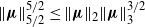 $\|\boldsymbol\mu\|_{5/2}^{5/2}\le \|\boldsymbol\mu\|_2\|\boldsymbol\mu\|_3^{3/2}$
. Applying (48) with
$\|\boldsymbol\mu\|_{5/2}^{5/2}\le \|\boldsymbol\mu\|_2\|\boldsymbol\mu\|_3^{3/2}$
. Applying (48) with
 $s = \frac{3}{2}$
and
$s = \frac{3}{2}$
and
 $t = \frac{7}{2}$
to (46), we thus have
$t = \frac{7}{2}$
to (46), we thus have
 \begin{align*} A_5 = o\Big(\|\boldsymbol\mu\|_{2}^{{23}/{8}}\|\boldsymbol\mu\|_{{5}/{2}}^{{5}/{2}}\Big) = o\Big(\|\boldsymbol\mu\|_{2}^3\|\boldsymbol\mu\|_{{5}/{2}}^{{5}/{2}}\Big) = o\Big(\|\boldsymbol\mu\|_{2}^{4}\|\boldsymbol\mu\|_3^{{3}/{2}}\Big), \end{align*}
which also matches (47). This proves (45) for
 $\ell=5$
, and completes the proof of Theorem 2.
$\ell=5$
, and completes the proof of Theorem 2.
Acknowledgements
We wish to thank two anonymous referees for their constructive comments that helped improve the quality of the paper.
Funding information
There are no funding bodies to thank relating to the creation of this article.
Competing interests
There were no competing interests to declare which arose during the preparation or publication process of this article.


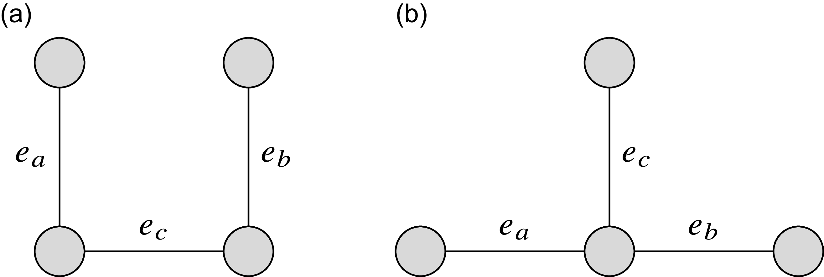


 Open access