


1 Introduction
In this article, we address the following question: Is it possible to determine the non-linear law of a reaction-diffusion process by applying sources and measuring the corresponding flux on the boundary of the domain of diffusion? Mathematically, the question can be stated as a problem of determination of a general semilinear term appearing in a semilinear parabolic equation from boundary measurements.
Let us explain the problem precisely. Let $T>0$
and
$T>0$
and $\Omega \subset {\mathbb R}^n$
, with
$\Omega \subset {\mathbb R}^n$
, with $n\geqslant 2$
, be a bounded and connected domain with a smooth boundary. Let
$n\geqslant 2$
, be a bounded and connected domain with a smooth boundary. Let $a:=(a_{ik})_{1 \leqslant i,k \leqslant n} \in C^\infty ([0,T]\times \overline {\Omega };{\mathbb R}^{n\times n})$
be symmetric matrix field,
$a:=(a_{ik})_{1 \leqslant i,k \leqslant n} \in C^\infty ([0,T]\times \overline {\Omega };{\mathbb R}^{n\times n})$
be symmetric matrix field,
 $$ \begin{align*}a_{ik}(t,x)=a_{ki}(t,x),\ x \in \Omega,\ i,k = 1,\ldots,n, \ (t,x)\in [0,T]\times\overline{\Omega}, \end{align*} $$
which fulfills the following ellipticity condition: there exists a constant $c>0$
such that
$c>0$
such that
 $$ \begin{align} \sum_{i,k=1}^n a_{ik}(t,x) \xi_i \xi_k \geqslant c |\xi|^2, \quad \mbox{for each } (t,x)\in [0,T]\times\overline{\Omega},\ \xi=(\xi_1,\ldots,\xi_n) \in {\mathbb R}^n. \end{align} $$
We define elliptic operators $\mathcal A(t)$
,
$\mathcal A(t)$
, $t\in [0,T]$
, in divergence form by
$t\in [0,T]$
, in divergence form by
 $$ \begin{align*}\mathcal A(t) u(t,x) :=-\sum_{i,k=1}^n \partial_{x_i} \left( a_{ik}(t,x) \partial_{x_k} u(t,x) \right),\ x\in\overline{\Omega},\ t\in[0,T]. \end{align*} $$
Throughout the article, we set
 $$ \begin{align*}Q:= (0,T) \times \Omega, \quad \Sigma := (0,T) \times \partial\Omega, \end{align*} $$
and we refer to $\Sigma $
as the lateral boundary. Let us also fix
$\Sigma $
as the lateral boundary. Let us also fix $\rho \in C^\infty ([0,T]\times \overline {\Omega };{\mathbb R}_+)$
and
$\rho \in C^\infty ([0,T]\times \overline {\Omega };{\mathbb R}_+)$
and $b\in C^\infty ([0,T]\times \overline {\Omega }\times {\mathbb R})$
. Here,
$b\in C^\infty ([0,T]\times \overline {\Omega }\times {\mathbb R})$
. Here, ${\mathbb R}_+=(0,+\infty )$
. Then, we consider the following initial boundary value problem (IBVP in short):
${\mathbb R}_+=(0,+\infty )$
. Then, we consider the following initial boundary value problem (IBVP in short):
 $$ \begin{align} \begin{cases} \rho(t,x) \partial_t u(t,x)+\mathcal A(t) u(t,x)+ b(t,x,u(t,x)) = 0, & (t,x)\in Q,\\ u(t,x) = f(t,x), & (t,x) \in \Sigma, \\ u(0,x) = 0, & x \in \Omega. \end{cases} \end{align} $$
The parabolic Dirichlet-to-Neumann map (DN map in short) is formally defined by
 $$ \begin{align*}\mathcal N_{b}: f\mapsto \left.\partial_{\nu(a)} u \right|{}_\Sigma, \end{align*} $$
where u is the solution to (1.2). Here, the conormal derivative $\partial _{\nu (a)}$
associated to the coefficient a is defined by
$\partial _{\nu (a)}$
associated to the coefficient a is defined by
 $$ \begin{align*}\partial_{\nu(a)}v(t,x):=\sum_{i,k=1}^na_{ik}(t,x)\partial_{x_k}v(t,x)\nu_i(x),\quad (t,x)\in\Sigma,\end{align*} $$
where $\nu =(\nu _1,\ldots ,\nu _n)$
denotes the outward unit normal vector of
$\nu =(\nu _1,\ldots ,\nu _n)$
denotes the outward unit normal vector of $\partial \Omega $
with respect to the Euclidean
$\partial \Omega $
with respect to the Euclidean ${\mathbb R}^n$
metric. The solution u used in the definition of the DN map
${\mathbb R}^n$
metric. The solution u used in the definition of the DN map $\mathcal {N}_b$
is unique in a specific sense so that there is no ambiguity in the definition of
$\mathcal {N}_b$
is unique in a specific sense so that there is no ambiguity in the definition of $\mathcal {N}_b$
. For this fact and a rigorous definition of the DN map, we refer to to Section 2.1. We write simply
$\mathcal {N}_b$
. For this fact and a rigorous definition of the DN map, we refer to to Section 2.1. We write simply $\partial _{\nu }=\partial _{\nu (a)}$
in the case a is the
$\partial _{\nu }=\partial _{\nu (a)}$
in the case a is the $n\times n$
identity matrix
$n\times n$
identity matrix $\mathrm {Id}_{{\mathbb R}^{n\times n}}$
. The inverse problem we study is the following.
$\mathrm {Id}_{{\mathbb R}^{n\times n}}$
. The inverse problem we study is the following.
-
• Inverse problem (IP): Can we recover the semilinear term b from the knowledge of the parabolic Dirichlet-to-Neumann map $\mathcal N_{b}$
?
$\mathcal N_{b}$
?

Physically, reaction diffusion equations of the form (1.2) describe several classes of diffusion processes with applications in chemistry, biology, geology, physics and ecology. This includes the spreading of biological populations [Reference FisherFis37], the Rayleigh-Bénard convection [Reference Newell and WhiteheadNW87] or models appearing in combustion theory [Reference VolpertVol14, Reference Zeldovich and Frank-KamenetskyZFK38]. The inverse problem (IP) is equivalent to the determination of an underlying physical law of a diffusion process, described by the nonlinear expression b in (1.2), by applying different sources (e.g., heat sources) and measuring the corresponding flux at the lateral boundary $\Sigma $
. The information extracted from this way is encoded into the DN map
$\Sigma $
. The information extracted from this way is encoded into the DN map $\mathcal N_{b}$
.
$\mathcal N_{b}$
.
These last decades, problems of parameter identification in nonlinear partial differential equations have generated a large interest in the mathematical community. Among the different formulation of these inverse problems, the determination of a nonlinear law is one of the most challenging from the severe ill-posedness and nonlinearity of the problem. For diffusion equations, one of the first results in that direction can be found in [Reference IsakovIsa93]. Later on, this result was improved by [Reference Choulli and KianCK18b], where the stability issue was also considered. To the best of our knowledge, the most general and complete result known so far about the determination of a semilinear term of the form $b(t,x,u)$
depending simultaneously on the time variable t, the space variable x and the solution of the equation u from knowledge of the parabolic DN map
$b(t,x,u)$
depending simultaneously on the time variable t, the space variable x and the solution of the equation u from knowledge of the parabolic DN map $\mathcal N_{b}$
can be found in [Reference Kian and UhlmannKU23]. Without being exhaustive, we mention the works of [Reference IsakovIsa01, Reference Cannon and YinCY88, Reference Choulli, Ouhabaz and YamamotoCOY06] devoted to the determination of semilinear terms depending only on the solution and the determination of quasilinear terms addressed in [Reference Caro and KianCK18a, Reference Egger, Pietschmann and SchlottbomEPS17, Reference Feizmohammadi, Kian and UhlmannFKU22]. Finally, we mention the works of [Reference Feizmohammadi and OksanenFO20, Reference Kurylev, Lassas and UhlmannKLU18, Reference Lassas, Liimatainen, Lin and SaloLLLS21, Reference Lassas, Liimatainen, Lin and SaloLLLS20, Reference Liimatainen, Lin, Salo and TyniLLST22, Reference Krupchyk and UhlmannKU20b, Reference Krupchyk and UhlmannKU20a, Reference Feizmohammadi, Liimatainen and LinFLL23, Reference Harrach and LinHL23, Reference Kian, Krupchyk and UhlmannKKU23, Reference Cârstea, Feizmohammadi, Kian, Krupchyk and UhlmannCFK+21, Reference Feizmohammadi, Kian and UhlmannFKU22, Reference Lai and LinLL22a, Reference LinLin22, Reference Kian and UhlmannKU23, Reference Lin and LiuLL23, Reference Lai and LinLL19] devoted to similar problems for elliptic and hyperbolic equations. Moreover, in the recent works [Reference Lin, Liu, Liu and ZhangLLLZ22, Reference Lin, Liu and LiuLLL21], the authors investigated simultaneous determination problems of coefficients and initial data for both parabolic and hyperbolic equations.
$\mathcal N_{b}$
can be found in [Reference Kian and UhlmannKU23]. Without being exhaustive, we mention the works of [Reference IsakovIsa01, Reference Cannon and YinCY88, Reference Choulli, Ouhabaz and YamamotoCOY06] devoted to the determination of semilinear terms depending only on the solution and the determination of quasilinear terms addressed in [Reference Caro and KianCK18a, Reference Egger, Pietschmann and SchlottbomEPS17, Reference Feizmohammadi, Kian and UhlmannFKU22]. Finally, we mention the works of [Reference Feizmohammadi and OksanenFO20, Reference Kurylev, Lassas and UhlmannKLU18, Reference Lassas, Liimatainen, Lin and SaloLLLS21, Reference Lassas, Liimatainen, Lin and SaloLLLS20, Reference Liimatainen, Lin, Salo and TyniLLST22, Reference Krupchyk and UhlmannKU20b, Reference Krupchyk and UhlmannKU20a, Reference Feizmohammadi, Liimatainen and LinFLL23, Reference Harrach and LinHL23, Reference Kian, Krupchyk and UhlmannKKU23, Reference Cârstea, Feizmohammadi, Kian, Krupchyk and UhlmannCFK+21, Reference Feizmohammadi, Kian and UhlmannFKU22, Reference Lai and LinLL22a, Reference LinLin22, Reference Kian and UhlmannKU23, Reference Lin and LiuLL23, Reference Lai and LinLL19] devoted to similar problems for elliptic and hyperbolic equations. Moreover, in the recent works [Reference Lin, Liu, Liu and ZhangLLLZ22, Reference Lin, Liu and LiuLLL21], the authors investigated simultaneous determination problems of coefficients and initial data for both parabolic and hyperbolic equations.
Most of the above mentioned results concern the inverse problem (IP) under the assumption that the semilinear term b in (1.2) satisfies the condition
 $$ \begin{align} b(t,x,0)=0,\quad (t,x)\in Q. \end{align} $$
This condition implies that (1.2) has at least one known solution, the trivial solution. In the same spirit, for any constant $\lambda \in {\mathbb R}$
, the condition
$\lambda \in {\mathbb R}$
, the condition $ b(t,x,\lambda )=0$
for
$ b(t,x,\lambda )=0$
for $(t,x)\in Q$
implies that the constant function
$(t,x)\in Q$
implies that the constant function $(t,x)\mapsto \lambda $
is a solution of the equation
$(t,x)\mapsto \lambda $
is a solution of the equation $\rho (t,x) \partial _t u+\mathcal A(t) u+ b(t,x,u) = 0$
in Q. In the present article, we treat the determination of general class of semilinear terms that might not satisfy the condition (1.3). In this case, the inverse problem (IP) is even more challenging since no solutions of (1.2) may be known a priori. In fact, as observed in [Reference SunSun10] for elliptic equations, there is an obstruction to the determination of b from the knowledge of
$\rho (t,x) \partial _t u+\mathcal A(t) u+ b(t,x,u) = 0$
in Q. In the present article, we treat the determination of general class of semilinear terms that might not satisfy the condition (1.3). In this case, the inverse problem (IP) is even more challenging since no solutions of (1.2) may be known a priori. In fact, as observed in [Reference SunSun10] for elliptic equations, there is an obstruction to the determination of b from the knowledge of $\mathcal N_b$
in the form of a gauge symmetry. We demonstrate the gauge symmetry first in the form of an example.
$\mathcal N_b$
in the form of a gauge symmetry. We demonstrate the gauge symmetry first in the form of an example.
Example 1.1. Let us consider the inverse problem (IP) for the simplest linear case
 $$ \begin{align} \begin{cases} \partial_t u -\Delta u =b_0 &\text{ in }Q, \\ u=f& \text{ on }\Sigma,\\ u(0,x)=0 &\text{ in }\Omega, \end{cases} \end{align} $$
where the aim is to recover an unknown source term $b_0=b_0(x,t)$
. Here,
$b_0=b_0(x,t)$
. Here, $\Delta $
is the Laplacian, but it could also be replaced by a more general second-order elliptic operator whose coefficients are known. Let us consider a function
$\Delta $
is the Laplacian, but it could also be replaced by a more general second-order elliptic operator whose coefficients are known. Let us consider a function $\varphi \in C^{\infty }([0,T]\times \overline {\Omega })$
, which satisfies
$\varphi \in C^{\infty }([0,T]\times \overline {\Omega })$
, which satisfies $\varphi \not \equiv 0$
,
$\varphi \not \equiv 0$
, $\varphi (0,x)=0$
for
$\varphi (0,x)=0$
for $x\in \Omega $
and
$x\in \Omega $
and $\varphi =\partial _{\nu } \varphi =0$
on
$\varphi =\partial _{\nu } \varphi =0$
on $\Sigma $
, where
$\Sigma $
, where $\partial _\nu \varphi $
denotes the Neumann derivative of
$\partial _\nu \varphi $
denotes the Neumann derivative of $\varphi $
on
$\varphi $
on $\Sigma $
.
$\Sigma $
.
Then the function $\tilde u:=u+\varphi $
satisfies
$\tilde u:=u+\varphi $
satisfies
 $$ \begin{align} \begin{cases} \partial_t \tilde u -\Delta \tilde u =b_0+(\partial_t -\Delta)\varphi &\text{ in }Q, \\ \tilde u=f& \text{ on }\Sigma,\\ \tilde u(0,x)=0 &\text{ in }\Omega. \end{cases} \end{align} $$
Since u and $\tilde u$
have the same initial data at
$\tilde u$
have the same initial data at $t=0$
and boundary data on
$t=0$
and boundary data on $\Sigma $
, we see that the DN maps of (1.4) and (1.5) are the same. However, by unique continuation properties for parabolic equations (see, for example, [Reference Saut and ScheurerSS87, Theorem 1.1]), the conditions
$\Sigma $
, we see that the DN maps of (1.4) and (1.5) are the same. However, by unique continuation properties for parabolic equations (see, for example, [Reference Saut and ScheurerSS87, Theorem 1.1]), the conditions $\varphi =\partial _{\nu } \varphi =0$
on
$\varphi =\partial _{\nu } \varphi =0$
on $\Sigma $
and
$\Sigma $
and $\varphi \not \equiv 0$
imply that
$\varphi \not \equiv 0$
imply that $(\partial _t -\Delta )\varphi \not \equiv 0$
, and it follows that
$(\partial _t -\Delta )\varphi \not \equiv 0$
, and it follows that $b_0+(\partial _t -\Delta )\varphi \neq b_0$
. Consequently, the inverse problem (IP) cannot be uniquely solved.
$b_0+(\partial _t -\Delta )\varphi \neq b_0$
. Consequently, the inverse problem (IP) cannot be uniquely solved.
In what follows, we assume that $\alpha \in (0,1)$
and refer to Section 2.1 for the definitions of various function spaces that will show up. Let us describe the gauge symmetry, or gauge invariance, of the inverse problem (IP) in detail. For this, let a function
$\alpha \in (0,1)$
and refer to Section 2.1 for the definitions of various function spaces that will show up. Let us describe the gauge symmetry, or gauge invariance, of the inverse problem (IP) in detail. For this, let a function $\varphi \in C^{1+\frac {\alpha }{2},2+\alpha }([0,T]\times \overline {\Omega })$
again satisfy
$\varphi \in C^{1+\frac {\alpha }{2},2+\alpha }([0,T]\times \overline {\Omega })$
again satisfy
 $$ \begin{align} \varphi(0,x)=0,\quad x\in\Omega,\quad \varphi(t,x)=\partial_{\nu(a)} \varphi(t,x)=0,\quad (t,x)\in\Sigma, \end{align} $$
and consider the mapping $S_\varphi $
from
$S_\varphi $
from $ C^\infty ({\mathbb R};C^{\frac {\alpha }{2},\alpha }([0,T]\times \overline {\Omega }))$
into itself defined by
$ C^\infty ({\mathbb R};C^{\frac {\alpha }{2},\alpha }([0,T]\times \overline {\Omega }))$
into itself defined by
 $$ \begin{align} S_\varphi b(t,x,\mu)=b(t,x,\mu+\varphi(t,x))+\rho(t,x) \partial_t \varphi(t,x)+\mathcal A(t) \varphi(t,x),\quad (t,x,\mu)\in Q\times{\mathbb R}. \end{align} $$
As in the example above, one can easily check that $\mathcal N_{b}=\mathcal N_{S_\varphi b}$
.
$\mathcal N_{b}=\mathcal N_{S_\varphi b}$
.
In view of this obstruction, the inverse problem (IP) should be reformulated as a problem about determining the semilinear term up to the gauge symmetry described by (1.7). We note that (1.7) implies an equivalence relation for functions in $ C^\infty ({\mathbb R};C^{\frac {\alpha }{2},\alpha }([0,T]\times \overline {\Omega }))$
. Corresponding equivalence classes will be called gauge classes:
$ C^\infty ({\mathbb R};C^{\frac {\alpha }{2},\alpha }([0,T]\times \overline {\Omega }))$
. Corresponding equivalence classes will be called gauge classes:
Definition 1.1 (Gauge class).
We say that two nonlinearities $b_1,b_2\in C^\infty ({\mathbb R};C^{\frac {\alpha }{2},\alpha }([0,T]\times \overline {\Omega })$
are in the same gauge class, or equivalent up to a gauge, if there is
$b_1,b_2\in C^\infty ({\mathbb R};C^{\frac {\alpha }{2},\alpha }([0,T]\times \overline {\Omega })$
are in the same gauge class, or equivalent up to a gauge, if there is $\varphi \in C^{1+\frac {\alpha }{2},2+\alpha }([0,T]\times \overline {\Omega })$
satisfying (1.6) such that
$\varphi \in C^{1+\frac {\alpha }{2},2+\alpha }([0,T]\times \overline {\Omega })$
satisfying (1.6) such that
 $$ \begin{align} b_1=S_\varphi b_2. \end{align} $$
Here, $S_\varphi $
is as in (1.7). In the case we consider a partial data inverse problem, where the normal derivative of solutions is assumed to be known only on
$S_\varphi $
is as in (1.7). In the case we consider a partial data inverse problem, where the normal derivative of solutions is assumed to be known only on $(0,T)\times \tilde \Gamma $
, with
$(0,T)\times \tilde \Gamma $
, with $\tilde \Gamma $
open in
$\tilde \Gamma $
open in $\partial \Omega $
, we assume
$\partial \Omega $
, we assume $\partial _{\nu (a)} \varphi =0$
only on
$\partial _{\nu (a)} \varphi =0$
only on $(0,T)\times \tilde \Gamma $
in (1.6).
$(0,T)\times \tilde \Gamma $
in (1.6).
Using the above definition of the gauge class and taking into account the obstruction described above, we reformulate the inverse problem (IP) as follows.
-
• Inverse problem (IP1): Can we determine the gauge class of the semilinear term b from the full or a partial knowledge of the parabolic DN map
$\mathcal N_{b}$
?

There is a natural additional question raised by (IP1) – namely,
-
• Inverse problem (IP2): When does the gauge invariance break leading to a full resolution of the inverse problem (IP)?
One can easily check that it is possible to give a positive answer to problem (IP2) when (1.3) is fulfilled. Nevertheless, as observed in the recent work [Reference Liimatainen and LinLL22b], the resolution of problem (IP2) is not restricted to such situations. The work [Reference Liimatainen and LinLL22b] provided the first examples (in an elliptic setting) how to use nonlinearity as a tool to break the gauge invariance of (IP).
Let us also remark that, following Example 1.1, when $u\mapsto b(\,\cdot \,,u)$
is affine, corresponding to the case where the equation (1.2) is linear and has a source term, there is no hope to break the gauge invariance (1.7) and the answer to (IP2) is, in general, negative. As will be observed in this article, this is no longer the case for various classes of nonlinear terms b. We will present cases where we will be able to solve (IP) uniquely. These cases present new instances where nonlinear interaction can be helpful in inverse problems. Nonlinearity has earlier been observed to be a helpful tool by many authors in different situations such as in partial data inverse problems and in anisotropic inverse problems on manifolds; see, for example, [Reference Kurylev, Lassas and UhlmannKLU18, Reference Feizmohammadi and OksanenFO20, Reference Lassas, Liimatainen, Lin and SaloLLLS21, Reference Lassas, Liimatainen, Lin and SaloLLLS20, Reference Liimatainen, Lin, Salo and TyniLLST22, Reference Krupchyk and UhlmannKU20a, Reference Krupchyk and UhlmannKU20b, Reference Feizmohammadi, Liimatainen and LinFLL23].
$u\mapsto b(\,\cdot \,,u)$
is affine, corresponding to the case where the equation (1.2) is linear and has a source term, there is no hope to break the gauge invariance (1.7) and the answer to (IP2) is, in general, negative. As will be observed in this article, this is no longer the case for various classes of nonlinear terms b. We will present cases where we will be able to solve (IP) uniquely. These cases present new instances where nonlinear interaction can be helpful in inverse problems. Nonlinearity has earlier been observed to be a helpful tool by many authors in different situations such as in partial data inverse problems and in anisotropic inverse problems on manifolds; see, for example, [Reference Kurylev, Lassas and UhlmannKLU18, Reference Feizmohammadi and OksanenFO20, Reference Lassas, Liimatainen, Lin and SaloLLLS21, Reference Lassas, Liimatainen, Lin and SaloLLLS20, Reference Liimatainen, Lin, Salo and TyniLLST22, Reference Krupchyk and UhlmannKU20a, Reference Krupchyk and UhlmannKU20b, Reference Feizmohammadi, Liimatainen and LinFLL23].
In the present article, we will address both problems (IP1) and (IP2). We will start by considering the problem (IP1) for nonlinear terms, which are quite general. Then, we will exhibit several general situations where the gauge invariance breaks and give an answer to (IP2).
We mainly restrict our analysis to semilinear terms b subjected to the condition that the map $u\mapsto b(\,\cdot \,,u)$
is analytic (the
$u\mapsto b(\,\cdot \,,u)$
is analytic (the $(t,x)$
dependence is of
$(t,x)$
dependence is of $b(t,x,\mu )$
will not be assumed to be analytic). The restriction to this class of nonlinear terms is motivated by the study of the challenging problems (IP1) and (IP2) in this article. Indeed, even when condition (1.3) is fulfilled, the problem (IP) is still open, in general, for semilinear terms that are not subjected to our analyticity condition (see [Reference Kian and UhlmannKU23] for the most complete results known so far for this problem). Results for semilinear elliptic equations have also been proven for cases when the nonlinear terms are, roughly speaking, globally Lipschitz (see, for example, [Reference Isakov and NachmanIN95, Reference Isakov and SylvesterIS94]). For this reason, our assumptions seem reasonable for tackling problems (IP1) and (IP2) and giving the first answers to these challenging problems. Note also that the linear part of (1.2) will be associated with a general class of linear parabolic equations with variable time-dependent coefficients. Consequently, we will present results also for linear equations with full and partial data measurements.
$b(t,x,\mu )$
will not be assumed to be analytic). The restriction to this class of nonlinear terms is motivated by the study of the challenging problems (IP1) and (IP2) in this article. Indeed, even when condition (1.3) is fulfilled, the problem (IP) is still open, in general, for semilinear terms that are not subjected to our analyticity condition (see [Reference Kian and UhlmannKU23] for the most complete results known so far for this problem). Results for semilinear elliptic equations have also been proven for cases when the nonlinear terms are, roughly speaking, globally Lipschitz (see, for example, [Reference Isakov and NachmanIN95, Reference Isakov and SylvesterIS94]). For this reason, our assumptions seem reasonable for tackling problems (IP1) and (IP2) and giving the first answers to these challenging problems. Note also that the linear part of (1.2) will be associated with a general class of linear parabolic equations with variable time-dependent coefficients. Consequently, we will present results also for linear equations with full and partial data measurements.
2 Main results
In this section, we will first introduce some preliminary definitions and results required for the rigorous formulation of our problem (IP). Then, we will state our main results for problems (IP1) and (IP2).
2.1 Preliminary properties
From now on, we fix $\alpha \in (0,1)$
, and we denote by
$\alpha \in (0,1)$
, and we denote by $C^{\frac {\alpha }{2},\alpha }([0,T]\times X)$
, with
$C^{\frac {\alpha }{2},\alpha }([0,T]\times X)$
, with $X=\overline {\Omega }$
or
$X=\overline {\Omega }$
or $X=\partial \Omega $
, the set of functions h lying in
$X=\partial \Omega $
, the set of functions h lying in $ C([0,T]\times X)$
satisfying
$ C([0,T]\times X)$
satisfying
 $$ \begin{align*}[h]_{\frac{\alpha}{2},\alpha}=\sup\left\{\frac{|h(t,x)-h(s,y)|}{(|x-y|^2+|t-s|)^{\frac{\alpha}{2}}}:\, (t,x),(s,y)\in [0,T]\times X,\ (t,x)\neq(s,y)\right\}<\infty.\end{align*} $$
Then we define the space $ C^{1+\frac {\alpha }{2},2+\alpha }([0,T]\times X)$
as the set of functions h lying in
$ C^{1+\frac {\alpha }{2},2+\alpha }([0,T]\times X)$
as the set of functions h lying in
 $$ \begin{align*}C([0,T];C^2(X))\cap C^1([0,T];C(X))\end{align*} $$
such that
 $$ \begin{align*}\partial_th,\partial_x^\beta h\in C^{\frac{\alpha}{2},\alpha}([0,T]\times X),\quad \beta\in(\mathbb N\cup\{0\})^n,\ |\beta|=2.\end{align*} $$
We consider these spaces with their usual norms, and we refer to [Reference ChoulliCho09, pp. 4] for more details. Let us also introduce the space
 $$ \begin{align*}\mathcal K_0:=\left\{h\in C^{1+\frac{\alpha}{2},2+\alpha}([0,T]\times\partial\Omega):\, h(0,\,\cdot\,)=\partial_th(0,\,\cdot\,)= 0\right\}.\end{align*} $$
If $r>0$
and
$r>0$
and $h\in \mathcal K_0$
, we denote by
$h\in \mathcal K_0$
, we denote by
 $$ \begin{align} \mathbb B(h,r):= \left\{ g\in \mathcal{K}_0:\, \left\lVert g-h\right\rVert_{C^{1+\frac{\alpha}{2},2+\alpha}([0,T]\times\partial\Omega)}<r \right\} \end{align} $$
the ball centered at h and of radius r in the space $\mathcal K_0$
. We assume also that b fulfills the following condition:
$\mathcal K_0$
. We assume also that b fulfills the following condition:
 $$ \begin{align} b(0,x,0)=0,\quad x\in\partial\Omega. \end{align} $$
In this article, we assume that there exists $f_0\in \mathcal K_0$
such that (1.2) admits a unique solution u lying in
$f_0\in \mathcal K_0$
such that (1.2) admits a unique solution u lying in $C^{1+\frac {\alpha }{2},2+\alpha }([0,T]\times \overline {\Omega })$
when
$C^{1+\frac {\alpha }{2},2+\alpha }([0,T]\times \overline {\Omega })$
when $f=f_0$
. We note that the existence of u requires the condition (2.2) in order to have compatibility with the initial data at time
$f=f_0$
. We note that the existence of u requires the condition (2.2) in order to have compatibility with the initial data at time $t=0$
and the Dirichlet data on the lateral boundary
$t=0$
and the Dirichlet data on the lateral boundary $\Sigma $
(see [Reference Ladyženskaja, Solonnikov and Ural’cevaLSU88, pp. 319 and pp. 449] for more details).
$\Sigma $
(see [Reference Ladyženskaja, Solonnikov and Ural’cevaLSU88, pp. 319 and pp. 449] for more details).
According to [Reference Ladyženskaja, Solonnikov and Ural’cevaLSU88, Theorem 6.1, pp. 452], [Reference Ladyženskaja, Solonnikov and Ural’cevaLSU88, Theorem 2.2, pp. 429], [Reference Ladyženskaja, Solonnikov and Ural’cevaLSU88, Theorem 4.1, pp. 443], [Reference Ladyženskaja, Solonnikov and Ural’cevaLSU88, Lemma 3.1, pp. 535] and [Reference Ladyženskaja, Solonnikov and Ural’cevaLSU88, Theorem 5.4, pp. 448], the problem (1.2) is well-posed for any $f=f_0\in \mathcal K_0$
if, for instance, there exist
$f=f_0\in \mathcal K_0$
if, for instance, there exist $c_1,c_2\geqslant 0$
such that the semilinear term b satisfies the following sign condition
$c_1,c_2\geqslant 0$
such that the semilinear term b satisfies the following sign condition
 $$ \begin{align*}b(t,x,\mu)\mu\geqslant -c_1\mu^2-c_2,\quad t\in[0,T],\ x\in\overline{\Omega},\ \mu\in{\mathbb R}.\end{align*} $$
The unique existence of solutions of (1.2) for some $f\in \mathcal K_0$
is not restricted to such a situation. Indeed, assume that there exists
$f\in \mathcal K_0$
is not restricted to such a situation. Indeed, assume that there exists $\psi \in C^{1+\frac {\alpha }{2},2+\alpha }([0,T]\times \overline {\Omega })$
satisfying
$\psi \in C^{1+\frac {\alpha }{2},2+\alpha }([0,T]\times \overline {\Omega })$
satisfying
 $$ \begin{align*} \begin{cases} \rho(t,x) \partial_t \psi(t,x)+\mathcal A(t) \psi(t,x) = 0 & \text{ in } Q,\\ \psi(0,x) = 0 & \text{ for }x \in \Omega, \end{cases} \end{align*} $$
such that $b(t,x,\psi (t,x))=0$
for
$b(t,x,\psi (t,x))=0$
for $(t,x)\in [0,T]\times \overline {\Omega }$
. Then, one can easily check that (1.2) admits a unique solution when
$(t,x)\in [0,T]\times \overline {\Omega }$
. Then, one can easily check that (1.2) admits a unique solution when $f=\psi |_{\Sigma }$
. Moreover, applying Proposition 3.1, we deduce that (1.2) will be well-posed when
$f=\psi |_{\Sigma }$
. Moreover, applying Proposition 3.1, we deduce that (1.2) will be well-posed when $f\in \mathcal K_0$
is sufficiently close to
$f\in \mathcal K_0$
is sufficiently close to $\psi |_{\Sigma }$
in the sense of
$\psi |_{\Sigma }$
in the sense of $C^{1+\frac {\alpha }{2},2+\alpha }([0,T]\times \partial \Omega )$
.
$C^{1+\frac {\alpha }{2},2+\alpha }([0,T]\times \partial \Omega )$
.
As will be shown in Proposition 3.1, the existence of $f_0\in \mathcal K_0$
such that (1.2) admits a solution when
$f_0\in \mathcal K_0$
such that (1.2) admits a solution when $f=f_0$
implies that there exists
$f=f_0$
implies that there exists $\epsilon>0$
, depending on a,
$\epsilon>0$
, depending on a, $\rho $
, b,
$\rho $
, b, $f_0$
,
$f_0$
, $\Omega $
, T, such that, for all
$\Omega $
, T, such that, for all $f\in \mathbb B(f_0,\epsilon )$
, the problem (1.2) admits a solution
$f\in \mathbb B(f_0,\epsilon )$
, the problem (1.2) admits a solution $u_f\in C^{1+\frac {\alpha }{2},2+\alpha }([0,T]\times \overline {\Omega })$
, which is unique in a sufficiently small neighborhood of the solution of (1.2) with boundary value
$u_f\in C^{1+\frac {\alpha }{2},2+\alpha }([0,T]\times \overline {\Omega })$
, which is unique in a sufficiently small neighborhood of the solution of (1.2) with boundary value $f=f_0$
. Using these properties, we can define the parabolic DN map
$f=f_0$
. Using these properties, we can define the parabolic DN map
 $$ \begin{align} \mathcal N_{b}:\mathbb B(f_0,\epsilon)\ni f\mapsto \partial_{\nu(a)} u_f(t,x),\quad (t,x)\in\Sigma. \end{align} $$
2.2 Resolution of (IP1)
We present our first main results about recovering the gauge class of a semilinear term from the corresponding DN map.
We consider $\Omega _1$
to be an open bounded, smooth and connected subset of
$\Omega _1$
to be an open bounded, smooth and connected subset of ${\mathbb R}^n$
such that
${\mathbb R}^n$
such that $\overline {\Omega }\subset \Omega _1$
. We extend a and
$\overline {\Omega }\subset \Omega _1$
. We extend a and $\rho $
into functions defined smoothly on
$\rho $
into functions defined smoothly on $[0,T]\times \overline {\Omega }_1$
satisfying
$[0,T]\times \overline {\Omega }_1$
satisfying $\rho>0$
and condition (1.1) with
$\rho>0$
and condition (1.1) with $\Omega $
replaced by
$\Omega $
replaced by $\Omega _1$
. For all
$\Omega _1$
. For all $t\in [0,T]$
, we set also
$t\in [0,T]$
, we set also
 $$ \begin{align*}g(t):=\rho(t,\,\cdot\,)a(t,\,\cdot\,)^{-1}, \end{align*} $$
and we consider the compact Riemannian manifold with boundary $(\overline {\Omega }_1,g(t))$
.
$(\overline {\Omega }_1,g(t))$
.
Assumption 2.1. Throughout this article, we assume that $ (\overline {\Omega }_1,g(t) )$
is a simple Riemannian manifold for all
$ (\overline {\Omega }_1,g(t) )$
is a simple Riemannian manifold for all $t\in [0,T]$
. That is, we assume that for any point
$t\in [0,T]$
. That is, we assume that for any point $x\in \overline {\Omega }_1$
, the exponential map
$x\in \overline {\Omega }_1$
, the exponential map $\exp _x$
is a diffeomorphism from some closed neighborhood of
$\exp _x$
is a diffeomorphism from some closed neighborhood of $0$
in
$0$
in $T_x\hspace {0.5pt} \overline {\Omega }_1$
onto
$T_x\hspace {0.5pt} \overline {\Omega }_1$
onto $\overline {\Omega }_1$
and
$\overline {\Omega }_1$
and $\partial \Omega _1$
is strictly convex.
$\partial \Omega _1$
is strictly convex.
From now on, for any Banach space X, we denote by $\mathbb A({\mathbb R};X)$
the set of analytic functions on
$\mathbb A({\mathbb R};X)$
the set of analytic functions on ${\mathbb R}$
as maps taking values in X. That is, for any
${\mathbb R}$
as maps taking values in X. That is, for any $b\in \mathbb A({\mathbb R};X)$
and
$b\in \mathbb A({\mathbb R};X)$
and $\mu \in {\mathbb R}$
, b has convergent X-valued Taylor series on a neighborhood of
$\mu \in {\mathbb R}$
, b has convergent X-valued Taylor series on a neighborhood of $\mu $
.
$\mu $
.
Theorem 2.1. Let $a:=(a_{ik})_{1 \leqslant i,k \leqslant n} \in C^\infty ([0,T]\times \overline {\Omega };{\mathbb R}^{n\times n})$
satisfy (1.1) and
$a:=(a_{ik})_{1 \leqslant i,k \leqslant n} \in C^\infty ([0,T]\times \overline {\Omega };{\mathbb R}^{n\times n})$
satisfy (1.1) and $\rho \in C^\infty ([0,T]\times \overline {\Omega };{\mathbb R}_+)$
. Let
$\rho \in C^\infty ([0,T]\times \overline {\Omega };{\mathbb R}_+)$
. Let $b_j\in \mathbb A({\mathbb R};C^{\frac {\alpha }{2},\alpha }([0,T]\times \overline {\Omega }))$
, which satisfies (2.2) as
$b_j\in \mathbb A({\mathbb R};C^{\frac {\alpha }{2},\alpha }([0,T]\times \overline {\Omega }))$
, which satisfies (2.2) as $b=b_j$
, for
$b=b_j$
, for $j=1,2$
. We also assume that there exists
$j=1,2$
. We also assume that there exists $f_0\in \mathcal K_0$
such that problem (1.2), with
$f_0\in \mathcal K_0$
such that problem (1.2), with $f=f_0$
and
$f=f_0$
and $b=b_j$
, admits a unique solution for
$b=b_j$
, admits a unique solution for $j=1,2$
. Then, the condition
$j=1,2$
. Then, the condition
 $$ \begin{align} \mathcal N_{b_1}(f)=\mathcal N_{b_2}(f),\quad f\in \mathbb B(f_0,\epsilon) \end{align} $$
implies that there exists $\varphi \in C^{1+\frac {\alpha }{2},2+\alpha }([0,T]\times \overline {\Omega })$
satisfying (1.6) such that
$\varphi \in C^{1+\frac {\alpha }{2},2+\alpha }([0,T]\times \overline {\Omega })$
satisfying (1.6) such that
 $$ \begin{align} b_1=S_\varphi b_2 \end{align} $$
with $S_\varphi $
the map defined by (1.7).
$S_\varphi $
the map defined by (1.7).
Remark 2.1. Let us list the data that can be recovered by our methods without the assumption of analyticity of b in the $\mu $
-variable. In this case, we can only recover the Taylor series of b in
$\mu $
-variable. In this case, we can only recover the Taylor series of b in $\mu $
-variable at shifted points. Indeed, assume as in Theorem 2.1 with the exception that the nonlinearities
$\mu $
-variable at shifted points. Indeed, assume as in Theorem 2.1 with the exception that the nonlinearities $b_1$
and
$b_1$
and $b_2$
are not analytic in the
$b_2$
are not analytic in the $\mu $
-variable, and fix
$\mu $
-variable, and fix $(t,x)$
. In this case, by inspecting the proof of Theorem 2.1(see Section 4), we can show that
$(t,x)$
. In this case, by inspecting the proof of Theorem 2.1(see Section 4), we can show that
 $$\begin{align*}\partial_\mu^k\hspace{0.5pt} b_1\left(t,x,u_{1,0}(t,x)\right)=\partial_\mu^k\hspace{0.5pt} b_2\left(t,x,u_{2,0}(t,x)\right),\quad \text{ for any } k\in \mathbb N, \end{align*}$$
where $u_{j,0}(t,x)$
, for
$u_{j,0}(t,x)$
, for $j=1,2$
, is the solution to (1.2) with coefficient
$j=1,2$
, is the solution to (1.2) with coefficient $b=b_j$
and boundary value
$b=b_j$
and boundary value $f=f_0\in \mathcal {K}_0$
. Thus, we see that the formal Taylor series of
$f=f_0\in \mathcal {K}_0$
. Thus, we see that the formal Taylor series of $b_1(t,x,\,\cdot \,)$
at
$b_1(t,x,\,\cdot \,)$
at $u_{1,0}(t,x)$
is that of
$u_{1,0}(t,x)$
is that of $b_2(t,x,\,\cdot \,)$
shifted by
$b_2(t,x,\,\cdot \,)$
shifted by $u_{2,0}(t,x)-u_{1,0}(t,x)$
, which is typically nonzero as we do not assume that we know any solutions to (1.2) a priori.
$u_{2,0}(t,x)-u_{1,0}(t,x)$
, which is typically nonzero as we do not assume that we know any solutions to (1.2) a priori.
By assuming analyticity in Theorem 2.1, we are able to connect the Taylor series of $b_1$
and
$b_1$
and $b_2$
in the
$b_2$
in the $\mu $
-variable at different points, which leads to (2.5) in the end. This is one motivation for the analyticity assumption. Note that we do not assume analyticity in the other variables.
$\mu $
-variable at different points, which leads to (2.5) in the end. This is one motivation for the analyticity assumption. Note that we do not assume analyticity in the other variables.
For our second result, let us consider a partial data result when $\mathcal A(t)=-\Delta $
(that is,
$\mathcal A(t)=-\Delta $
(that is, $a=\text {Id}_{\hspace {0.5pt} {\mathbb R}^{n\times n}}$
is an
$a=\text {Id}_{\hspace {0.5pt} {\mathbb R}^{n\times n}}$
is an $n\times n$
identity matrix) and
$n\times n$
identity matrix) and $\rho \equiv 1$
. More precisely, consider the front and back sets of
$\rho \equiv 1$
. More precisely, consider the front and back sets of $\partial \Omega $
 $$ \begin{align*}\Gamma_\pm(x_0):=\left\{x\in\partial\Omega:\, \pm(x-x_0)\cdot\nu(x)\geqslant0 \right\}\end{align*} $$
with respect to a source $x_0\in {\mathbb R}^n\setminus \overline {\Omega }$
. Then, our second main result is stated as follows:
$x_0\in {\mathbb R}^n\setminus \overline {\Omega }$
. Then, our second main result is stated as follows:
Theorem 2.2. For $n\geqslant 3$
and
$n\geqslant 3$
and $\Omega $
simply connected, let
$\Omega $
simply connected, let $a=(a_{ik})_{1 \leqslant i,k \leqslant n}= \mathrm {Id}_{\,{\mathbb R}^{n\times n}}$
and
$a=(a_{ik})_{1 \leqslant i,k \leqslant n}= \mathrm {Id}_{\,{\mathbb R}^{n\times n}}$
and $\rho \equiv 1$
. Let
$\rho \equiv 1$
. Let $b_j\in \mathbb A({\mathbb R};C^{\frac {\alpha }{2},\alpha }([0,T]\times \overline {\Omega }))$
, which satisfies (2.2) as
$b_j\in \mathbb A({\mathbb R};C^{\frac {\alpha }{2},\alpha }([0,T]\times \overline {\Omega }))$
, which satisfies (2.2) as $b=b_j$
, for
$b=b_j$
, for $j=1,2$
. We also assume that there exists
$j=1,2$
. We also assume that there exists $f_0\in \mathcal K_0$
such that problem (1.2), with
$f_0\in \mathcal K_0$
such that problem (1.2), with $f=f_0$
and
$f=f_0$
and $b=b_j$
, admits a unique solution, for
$b=b_j$
, admits a unique solution, for $j=1,2$
. Fix
$j=1,2$
. Fix $x_0\in {\mathbb R}^n\setminus \overline {\Omega }$
and consider
$x_0\in {\mathbb R}^n\setminus \overline {\Omega }$
and consider $\tilde {\Gamma }$
a neighborhood of
$\tilde {\Gamma }$
a neighborhood of $\Gamma _-(x_0)$
on
$\Gamma _-(x_0)$
on $\partial \Omega $
. Then, the condition
$\partial \Omega $
. Then, the condition
 $$ \begin{align} \mathcal N_{b_1}f(t,x)=\mathcal N_{b_2}f(t,x),\quad (t,x)\in (0,T)\times \tilde{\Gamma}, \text{ for any } f\in\mathbb B(f_0,\epsilon) \end{align} $$
implies that there exists $\varphi \in C^{1+\frac {\alpha }{2},2+\alpha }([0,T]\times \overline {\Omega })$
satisfying
$\varphi \in C^{1+\frac {\alpha }{2},2+\alpha }([0,T]\times \overline {\Omega })$
satisfying
 $$ \begin{align} \varphi(0,x)=0,\quad x\in\Omega,\quad \varphi(t,x)=0,\quad (t,x)\in\Sigma, \end{align} $$
 $$ \begin{align} \partial_{\nu} \varphi(t,x)=0,\quad (t,x)\in (0,T)\times \tilde{\Gamma} \end{align} $$
such that
 $$ \begin{align} b_1=S_\varphi b_2. \end{align} $$
We will be able to break the gauge condition $b_1=S_\varphi b_2$
in Theorems 2.1 and 2.2 in various cases. We present these results separately in the next section.
$b_1=S_\varphi b_2$
in Theorems 2.1 and 2.2 in various cases. We present these results separately in the next section.
2.3 Breaking the gauge in the sense of (IP2)
In several situations, the gauge class (2.9) could be broken, and one can fully determine the semilinear term b in (1.2) from its parabolic DN map. We will present below classes of nonlinearities when such phenomenon occurs. We start by considering general elements of $b\in \mathbb A({\mathbb R};C^{\frac {\alpha }{2},\alpha }([0,T]\times \overline {\Omega }))$
for which the gauge invariance (2.9) breaks.
$b\in \mathbb A({\mathbb R};C^{\frac {\alpha }{2},\alpha }([0,T]\times \overline {\Omega }))$
for which the gauge invariance (2.9) breaks.
Corollary 2.1. Let the conditions of Theorem 2.1 be fulfilled and assume that there exists $\kappa \in C^{\frac {\alpha }{2},\alpha }([0,T]\times \overline {\Omega })$
such that
$\kappa \in C^{\frac {\alpha }{2},\alpha }([0,T]\times \overline {\Omega })$
such that
 $$ \begin{align} b_1(t,x,\kappa(t,x))=b_2(t,x,\kappa(t,x)),\quad (t,x)\in [0,T]\times\overline{\Omega}. \end{align} $$
Then, the condition (2.4) implies that $b_1=b_2$
. In the same way, assuming that the conditions of Theorem 2.2 are fulfilled, the condition (2.6) implies that
$b_1=b_2$
. In the same way, assuming that the conditions of Theorem 2.2 are fulfilled, the condition (2.6) implies that $b_1=b_2$
.
$b_1=b_2$
.
Corollary 2.2. Let the conditions of Theorem 2.1 be fulfilled, and assume that there exists $h\in C^{\alpha }(\overline {\Omega })$
,
$h\in C^{\alpha }(\overline {\Omega })$
, $G\in C^{\frac {\alpha }{2},\alpha }([0,T]\times \overline {\Omega })$
and
$G\in C^{\frac {\alpha }{2},\alpha }([0,T]\times \overline {\Omega })$
and $\theta \in (0,T]$
satisfying the condition
$\theta \in (0,T]$
satisfying the condition
 $$ \begin{align} \inf_{x\,{\in}\,\Omega}|G(\theta,x)|>0, \end{align} $$
such that
 $$ \begin{align} b_1(t,x,0)-b_2(t,x,0)=h(x)G(t,x),\quad (t,x)\in [0,T]\times\overline{\Omega}. \end{align} $$
Assume also that the solutions $u_{j,0}$
of (1.2),
$u_{j,0}$
of (1.2), $j=1,2$
, with
$j=1,2$
, with $f=f_0$
and
$f=f_0$
and $b=b_j$
, satisfy the condition
$b=b_j$
, satisfy the condition
 $$ \begin{align} u_{1,0}(\theta,x)=u_{2,0}(\theta,x),\quad x\in\Omega. \end{align} $$
Then, the condition (2.4) implies that $b_1=b_2$
. Moreover, by assuming that the conditions of Theorem 2.2 are fulfilled, the condition (2.6) implies that
$b_1=b_2$
. Moreover, by assuming that the conditions of Theorem 2.2 are fulfilled, the condition (2.6) implies that $b_1=b_2$
.
$b_1=b_2$
.
Now let us consider elements $b\in \mathbb A({\mathbb R};C^{\frac {\alpha }{2},\alpha }([0,T]\times \overline {\Omega }))$
which are polynomials of the form
$b\in \mathbb A({\mathbb R};C^{\frac {\alpha }{2},\alpha }([0,T]\times \overline {\Omega }))$
which are polynomials of the form
 $$ \begin{align} b(t,x,\mu)=\sum_{k=0}^N b_k(t,x)\mu^k,\quad (t,x,\mu)\in[0,T]\times\overline{\Omega}\times{\mathbb R}. \end{align} $$
For this class of nonlinear terms, we can prove the following.
Theorem 2.3. Let the condition of Theorem 2.1 be fulfilled, and assume that, for $j=1,2$
, there exists
$j=1,2$
, there exists $N_j\geqslant 2$
such that
$N_j\geqslant 2$
such that
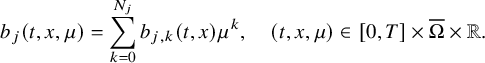 $$ \begin{align} b_j(t,x,\mu)=\sum_{k=0}^{N_j} b_{j,k}(t,x)\mu^k,\quad (t,x,\mu)\in[0,T]\times\overline{\Omega}\times{\mathbb R}. \end{align} $$
Let $\omega $
be an open subset of
$\omega $
be an open subset of ${\mathbb R}^n$
such that
${\mathbb R}^n$
such that $\omega \subset \Omega $
and J is a dense subset of
$\omega \subset \Omega $
and J is a dense subset of $(0,T)\times \omega $
. We assume also that, for
$(0,T)\times \omega $
. We assume also that, for $N=\min (N_1,N_2)$
, the conditions
$N=\min (N_1,N_2)$
, the conditions
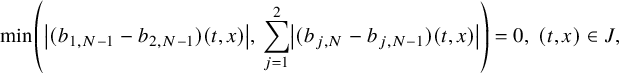 $$ \begin{align} \min\kern1pt \left(\left|(b_{1,N-1}-b_{2,N-1})(t,x)\right|, \, \sum_{j=1}^2\left|(b_{j,N}-b_{j,N-1})(t,x)\right|\right)=0,\ (t,x)\in J, \end{align} $$
 $$ \begin{align} \left|b_{1,N}(t,x)\right|>0,\quad (t,x)\in J \end{align} $$
 $$ \begin{align} b_{1,0}(t,x)=b_{2,0}(t,x),\quad (t,x)\in(0,T)\times(\Omega\setminus{\overline{\omega}}) \end{align} $$
hold true. Then the condition (2.4) implies that $b_1=b_2$
. In addition, assuming that the conditions of Theorem 2.2 are fulfilled, condition (2.6) implies that
$b_1=b_2$
. In addition, assuming that the conditions of Theorem 2.2 are fulfilled, condition (2.6) implies that $b_1=b_2$
.
$b_1=b_2$
.
We make the following remark.
Remark 2.2.
-
(i) The preceding theorem, in particular, says that the inverse source problem of recovering a source function F from the DN map of
is uniquely solvable. This is in strict contrast to the inverse source problem for the linear equation
$$\begin{align*}\partial_t u-\Delta u + u^2=F \end{align*}$$
$\partial _t u-\Delta u =F$
that always has a gauge invariance explained in Example 1.1: the sources F and
$\widetilde {F}:=F+\partial _t\varphi -\Delta \varphi $
in Q have the same DN map. Here, the only restrictions for
$\varphi $
are given in (1.6) and thus typically
$F\neq \widetilde F$
.
-
(ii) Inverse source problems for semilinear elliptic equations were studied in [Reference Liimatainen and LinLL22b]. There it was shown that if in the notation of the corollary
$b_{1,N-1}=b_{2,N-1}$
and
$b_{1,N}\neq 0$
in
$\Omega $
(so that (2.16) and (2.17) hold), then the gauge breaks. With natural replacements, the corollary generalizes [Reference Liimatainen and LinLL22b, Corollary 1.3] in the elliptic setting. This can be seen by inspecting its proof.


Let us then consider nonlinear terms $b\in \mathbb A({\mathbb R};C^{\frac {\alpha }{2},\alpha }([0,T]\times \overline {\Omega }))$
of the form
$b\in \mathbb A({\mathbb R};C^{\frac {\alpha }{2},\alpha }([0,T]\times \overline {\Omega }))$
of the form
 $$ \begin{align} b(t,x,\mu)=b_1(t,x)\hspace{0.5pt} h(t,b_2(t,x)\mu)+b_0(t,x),\quad (t,x,\mu)\in[0,T]\times\overline{\Omega}\times{\mathbb R}. \end{align} $$
We start by considering nonlinear terms of the form (2.19) with $b_2\equiv 1$
.
$b_2\equiv 1$
.
Theorem 2.4. Let the conditions of Theorem 2.1 be fulfilled, and assume that, for $j=1,2$
, there exists
$j=1,2$
, there exists $h_j\in \mathbb A({\mathbb R};C^{\frac {\alpha }{2}}([0,T]))$
such that
$h_j\in \mathbb A({\mathbb R};C^{\frac {\alpha }{2}}([0,T]))$
such that
 $$ \begin{align} b_j(t,x,\mu)=b_{j,1}(t,x)h_j(t,\mu)+b_{j,0}(t,x),\quad (t,x,\mu)\in[0,T]\times\overline{\Omega}\times{\mathbb R}. \end{align} $$
Assume also that, for all $t\in (0,T)$
, there exist
$t\in (0,T)$
, there exist $\mu _t\in {\mathbb R}$
and
$\mu _t\in {\mathbb R}$
and $n_t\in \mathbb N$
such that
$n_t\in \mathbb N$
such that
 $$ \begin{align} \partial_\mu^{n_t} h_1(t,\,\cdot\,)\not\equiv0 \text{ and } \partial_\mu^{n_t} h_1(t,\mu_t)=0,\quad t\in(0,T). \end{align} $$
Moreover, we assume that
 $$ \begin{align} b_{1,1}(t,x)\neq0,\quad (t,x)\in Q, \end{align} $$
and that for all $t\in (0,T)$
, there exists
$t\in (0,T)$
, there exists $x_t\in \partial \Omega $
such that
$x_t\in \partial \Omega $
such that
 $$ \begin{align} b_{1,1}(t,x_t)=b_{2,1}(t,x_t)\neq0,\quad t\in(0,T). \end{align} $$
Then, the condition (2.4) implies that $b_1=b_2$
. Moreover, assuming that the conditions of Theorem 2.2 are fulfilled, the condition (2.6) implies that
$b_1=b_2$
. Moreover, assuming that the conditions of Theorem 2.2 are fulfilled, the condition (2.6) implies that $b_1=b_2$
.
$b_1=b_2$
.
Under a stronger assumption imposed on the expression h, we can also consider nonlinear terms of the form (2.19) with $b_2\not \equiv 1$
.
$b_2\not \equiv 1$
.
Theorem 2.5. Let the conditions of Theorem 2.1 be fulfilled, and assume that, for $j=1,2$
, there exists
$j=1,2$
, there exists $h_j\in \mathbb A({\mathbb R};C^{\frac {\alpha }{2}}([0,T]))$
such that
$h_j\in \mathbb A({\mathbb R};C^{\frac {\alpha }{2}}([0,T]))$
such that
 $$ \begin{align} b_j(t,x,\mu)=b_{j,1}(t,x)h_j(t,b_{j,2}(t,x)\mu)+b_{j,0}(t,x),\quad (t,x,\mu)\in[0,T]\times\overline{\Omega}\times{\mathbb R}. \end{align} $$
Assume also that, for all $t\in (0,T)$
, there exists
$t\in (0,T)$
, there exists $n_t\in \mathbb N$
such that
$n_t\in \mathbb N$
such that
 $$ \begin{align} \partial_\mu^{n_t} h_1(t,\,\cdot\,)\not\equiv0 \text{ and } \partial_\mu^{n_t} h_1(t,0)=0,\quad t\in(0,T).\ \end{align} $$
Moreover, we assume that
 $$ \begin{align} b_{1,1}(t,x)\neq0 \text{ and } b_{1,2}(t,x)\neq0,\quad (t,x)\in Q, \end{align} $$
and that for all $t\in (0,T)$
, there exists
$t\in (0,T)$
, there exists $x_t\in \partial \Omega $
such that
$x_t\in \partial \Omega $
such that
 $$ \begin{align} b_{1,1}(t,x_t)=b_{2,1}(t,x_t)\neq0 \text{ and } b_{1,2}(t,x_t)=b_{2,2}(t,x_t)\neq0\quad t\in(0,T). \end{align} $$
Then, the condition (2.4) implies that $b_1=b_2$
. Moreover, assuming that the conditions of Theorem 2.2 are fulfilled, the condition (2.6) implies that
$b_1=b_2$
. Moreover, assuming that the conditions of Theorem 2.2 are fulfilled, the condition (2.6) implies that $b_1=b_2$
.
$b_1=b_2$
.
Finally, we consider nonlinear terms $b\in \mathbb A({\mathbb R};C^{\frac {\alpha }{2},\alpha }([0,T]\times \overline {\Omega }))$
satisfying
$b\in \mathbb A({\mathbb R};C^{\frac {\alpha }{2},\alpha }([0,T]\times \overline {\Omega }))$
satisfying
 $$ \begin{align} b(t,x,\mu)=b_1(t,x)G(x,b_2(t,x)\mu)+b_0(t,x),\quad (t,x,\mu)\in[0,T]\times\Omega\times{\mathbb R}. \end{align} $$
Corollary 2.3. Let the conditions of Theorem 2.1 be fulfilled, and assume that, for $j=1,2$
, there exists
$j=1,2$
, there exists $G\in \mathbb A({\mathbb R};C^{\alpha }(\overline {\Omega }))$
such that
$G\in \mathbb A({\mathbb R};C^{\alpha }(\overline {\Omega }))$
such that
 $$ \begin{align} b_j(t,x,\mu)=b_{j,1}(t,x)G(x,b_{j,2}(t,x)\mu)+b_{j,0}(t,x),\quad (t,x,\mu)\in[0,T]\times\Omega\times{\mathbb R}. \end{align} $$
Assume also that one of the following conditions is fulfilled:
-
(i) We have
$b_{1,2}=b_{2,2}$
, and for all
$x\in \Omega $
, there exists
$n_x\in \mathbb N$
and
$\mu _x\in {\mathbb R}$
such that (2.30)
$$ \begin{align} \partial_\mu^{n_x} G(x,\,\cdot\,)\not\equiv0 \text{ and } \partial_\mu^{n_x} G(x,\mu_x)=0,\quad x\in\Omega. \end{align} $$
-
(ii) For all
$x\in \Omega $
, there exists
$n_x\in \mathbb N$
such that (2.31)
$$ \begin{align} \partial_\mu^{n_x} G(x,\,\cdot\,)\not\equiv0\text{ and } \partial_\mu^{n_x} G(x,0)=0,\quad x\in\Omega. \end{align} $$


Moreover, we assume that condition (2.26) is fulfilled. Then, the condition (2.4) implies that $b_1=b_2$
. In addition, by assuming that the conditions of Theorem 2.2 are fulfilled, condition (2.6) implies that
$b_1=b_2$
. In addition, by assuming that the conditions of Theorem 2.2 are fulfilled, condition (2.6) implies that $b_1=b_2$
.
$b_1=b_2$
.
Remark 2.3. Let us observe that the results of Theorems 2.4 and 2.5 and Corollary 2.3 are mostly based on the conditions (2.21) and (2.26) imposed to nonlinear terms of the form (2.19), and on the conditions (2.30) and (2.31) imposed to nonlinear terms of the form (2.28). These conditions are rather general, and they will be fulfilled in various situations for different class of functions. For instance, assuming that the function $h_1$
takes the form
$h_1$
takes the form
 $$ \begin{align*}h_1(t,\mu)=P(t,\mu)\exp(Q(t,\mu)),\quad (t,\mu)\in[0,T]\times{\mathbb R}\end{align*} $$
with $P,Q\in \mathbb A({\mathbb R};C^{\frac {\alpha }{2}}([0,T]))$
, condition (2.21) will be fulfilled if we assume that there exists
$P,Q\in \mathbb A({\mathbb R};C^{\frac {\alpha }{2}}([0,T]))$
, condition (2.21) will be fulfilled if we assume that there exists $\sigma \in C^{\alpha /2}([0,T])$
such that
$\sigma \in C^{\alpha /2}([0,T])$
such that
 $$ \begin{align*}\left. \left(\partial_\mu P(t,\mu)+P(t,\mu)\partial_\mu Q(t,\mu)\right)\right|{}_{\mu=\sigma(t)}=0,\quad t\in[0,T].\end{align*} $$
Such a condition will, of course, be fulfilled when $h_1(t,\mu )=\mu e^\mu $
,
$h_1(t,\mu )=\mu e^\mu $
, $(t,\mu )\in [0,T]\times {\mathbb R}$
.
$(t,\mu )\in [0,T]\times {\mathbb R}$
.
More generally, let $\sigma \in C^{\frac {\alpha }{2}}([0,T])$
be arbitrary chosen, and for each
$\sigma \in C^{\frac {\alpha }{2}}([0,T])$
be arbitrary chosen, and for each $t\in [0,T]$
, consider
$t\in [0,T]$
, consider $N_t\in \mathbb N$
. Assuming that the function
$N_t\in \mathbb N$
. Assuming that the function $h_1$
satisfies the following property
$h_1$
satisfies the following property
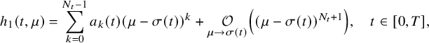 $$ \begin{align}h_1(t,\mu)=\sum_{k=0}^{N_t-1}a_k(t)(\mu-\sigma(t))^k+ \underset{\mu\to\sigma(t)}{\mathcal O}\left((\mu-\sigma(t))^{N_t+1}\right),\quad t\in[0,T],\end{align} $$
with $a_{k}\in C^{\frac {\alpha }{2}}([0,T])$
,
$a_{k}\in C^{\frac {\alpha }{2}}([0,T])$
, $k\in \mathbb N\cup \{0\}$
, one can easily check that condition (2.21) will be fulfilled since we have
$k\in \mathbb N\cup \{0\}$
, one can easily check that condition (2.21) will be fulfilled since we have
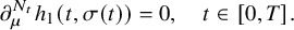 $$ \begin{align*}\partial_\mu^{N_t} h_1(t,\sigma(t))=0,\quad t\in[0,T].\end{align*} $$
Condition (2.26) will be fulfilled under the same condition provided that $h_1$
satisfies (2.32) with
$h_1$
satisfies (2.32) with $\sigma \equiv 0$
. Moreover, let
$\sigma \equiv 0$
. Moreover, let $g\in C^{\alpha }(\overline {\Omega })$
, and for each
$g\in C^{\alpha }(\overline {\Omega })$
, and for each $x\in \Omega $
, consider
$x\in \Omega $
, consider $N_x\in \mathbb N$
. Assuming that the function G in (2.30) satisfies the property
$N_x\in \mathbb N$
. Assuming that the function G in (2.30) satisfies the property
 $$ \begin{align}G(x,\mu)=\sum_{k=0}^{N_x-1}\beta_k(x)(\mu-g(x))^k+ \underset{\mu\to g(x)}{\mathcal O}\left((\mu-g(x))^{N_x+1}\right),\quad x\in \Omega,\end{align} $$
with functions $\beta _{k}\in C^{\alpha }(\overline {\Omega })$
,
$\beta _{k}\in C^{\alpha }(\overline {\Omega })$
, $k\in \mathbb N\cup \{0\}$
, it is clear that condition (2.30) will be fulfilled since we have
$k\in \mathbb N\cup \{0\}$
, it is clear that condition (2.30) will be fulfilled since we have
 $$ \begin{align*}\partial_\mu^{N_x} G(x,g(x))=0,\quad x\in \Omega.\end{align*} $$
The same is true for condition (2.31) when G satisfies (2.33) with $g\equiv 0$
.
$g\equiv 0$
.
Finally, via previous observations, we can also determine the order coefficients for linear parabolic equations.
Corollary 2.4 (Global uniqueness with partial data).
Adopting all notations in Theorem 2.2, let $q_j=q_j(t,x)\in C^\infty ([0,T]\times \overline {\Omega })$
and
$q_j=q_j(t,x)\in C^\infty ([0,T]\times \overline {\Omega })$
and $b_j(t,x,\mu )=q_j(t,x)\mu $
for
$b_j(t,x,\mu )=q_j(t,x)\mu $
for $j=1,2$
. Then (2.4) implies
$j=1,2$
. Then (2.4) implies $q_1=q_2$
in Q.
$q_1=q_2$
in Q.
We mention that we could also prove that the assumptions of Theorem 2.1 and $b_j(t,x,\mu )=q_j(t,x)\mu $
,
$b_j(t,x,\mu )=q_j(t,x)\mu $
, $j=1,2$
, imply
$j=1,2$
, imply $q_1=q_2$
.
$q_1=q_2$
.
2.4 Comments about our results
To the best of our knowledge, Theorems 2.1 and 2.2 give the first positive answer to the inverse problem (IP1) for semilinear parabolic equations. In addition, the results of Theorem 2.1 and 2.2 extend the analysis of [Reference Liimatainen and LinLL22b] that considered a problem similar to (IP1) for elliptic equations, but which did not fully answer the question raised by (IP1). In that sense, Theorems 2.1 and 2.2 give the first positive answer to (IP1) for a class of elliptic PDEs as well. While Theorem 2.1 is stated for general class of parabolic equations, Theorem 2.2 gives a result with measurements restricted to a neighborhood of the back set with respect to a source $x_0\in {\mathbb R}^n\setminus \overline {\Omega }$
in the spirit of the most precise partial data results stated for linear elliptic equations such as [Reference Kenig, Sjöstrand and UhlmannKSU07]. Note that in contrast to [Reference Kenig, Sjöstrand and UhlmannKSU07], the source
$x_0\in {\mathbb R}^n\setminus \overline {\Omega }$
in the spirit of the most precise partial data results stated for linear elliptic equations such as [Reference Kenig, Sjöstrand and UhlmannKSU07]. Note that in contrast to [Reference Kenig, Sjöstrand and UhlmannKSU07], the source $x_0$
is not necessary outside the convex hull of
$x_0$
is not necessary outside the convex hull of $\overline {\Omega }$
and, as observed in [Reference Kenig, Sjöstrand and UhlmannKSU07], when
$\overline {\Omega }$
and, as observed in [Reference Kenig, Sjöstrand and UhlmannKSU07], when $\Omega $
is convex, the measurements of Theorem 2.2 can be restricted to any open set of
$\Omega $
is convex, the measurements of Theorem 2.2 can be restricted to any open set of $\partial \Omega $
. Even for linear equations, Theorems 2.1 and 2.2 improve in precision and generality the earlier works of [Reference Choulli and KianCK18b, Reference IsakovIsa91] dealing with determination of time dependent coefficients appearing in linear parabolic equations.
$\partial \Omega $
. Even for linear equations, Theorems 2.1 and 2.2 improve in precision and generality the earlier works of [Reference Choulli and KianCK18b, Reference IsakovIsa91] dealing with determination of time dependent coefficients appearing in linear parabolic equations.
We gave a positive answer to the problem (IP2) and show that the gauge breaks for three different classes of semilinear terms:
-
1) Semilinear terms with prescribed information in Corollaries 2.1 and 2.2,
-
2) Polynomial semilinear terms in Theorem 2.3,
-
3) Semilinear terms with separated variables of the form (2.19) or (2.28) in Theorems 2.4 and 2.5 and in Corollary 2.3.
This seems to be the most complete overview of situations where one can give a positive answer to problem (IP2). While [Reference Liimatainen and LinLL22b] considered also such phenomena for polynomial nonlinear terms and some specific examples, the conditions of Corollary 2.1 and 2.2, Theorems 2.4 and 2.5 and Corollary 2.3, leading to a positive answer for (IP2), seem to be new. In Remark 2.3, we gave several concrete and general examples of semilinear terms satisfying the conditions of Theorems 2.4, 2.5 and Corollary 2.3.
The proof of our results is based on a combination of the higher-order linearization technique, application of suitable class of geometric optics solutions for parabolic equations, Carleman estimates, properties of holomorphic functions and different properties of parabolic equations. Theorem 2.1 is deduced from the linearized result of Proposition 4.1 that we prove by using geometric optics solutions for parabolic equations. These solutions are built by using the energy estimate approach introduced in the recent work of [Reference FeizmohammadiFei23].
We mention that Assumption 2.1 is used in this work mainly for two purposes. Our construction of geometric optics solutions is based on the use of global polar normal coordinates on the manifolds $(\overline {\Omega }_1, g(t) )$
,
$(\overline {\Omega }_1, g(t) )$
, $t\in [0,T]$
. In addition, Assumption 2.1 guarantees the injectivity of the geodesic ray transform on the manifolds
$t\in [0,T]$
. In addition, Assumption 2.1 guarantees the injectivity of the geodesic ray transform on the manifolds $ ( \overline {\Omega }_1, g(t))$
,
$ ( \overline {\Omega }_1, g(t))$
, $t\in [0,T]$
, which is required in our proofs of Theorems 2.1 and 2.2. It is not clear at the moment how Assumption 2.1 can be relaxed in the construction of geometric optics solutions for parabolic equations of the form considered in this paper.
$t\in [0,T]$
, which is required in our proofs of Theorems 2.1 and 2.2. It is not clear at the moment how Assumption 2.1 can be relaxed in the construction of geometric optics solutions for parabolic equations of the form considered in this paper.
This allows us to consider problem (IP1) for general class of semilinear parabolic equations with variable coefficients. In Theorem 2.2, we combine this class of geometric optics solutions with a Carleman estimate with boundary terms stated in Lemma 6.1 in order to restrict the boundary measurements to a part of the boundary. Note that the weight under consideration in Lemma 6.1 is not a limiting Carleman weight for parabolic equations. This is one reason why we cannot apply such Carleman estimates for making also a restriction on the support of the Dirichlet input in Theorem 2.2.
It is worth mentioning that our results for problem (IP1) and (IP2) can be applied to inverse source problems for nonlinear parabolic equations. This important application is discussed in Section 8. There we show how the nonlinear interaction allows to solve this problem for general classes of source terms, depending simultaneously on the time and space variables. Corresponding problems for linear equations cannot be solved uniquely (see Example 1.1 or, for example, [Reference Kian, Soccorsi, Xue and YamamotoKSXY22, Appendix A]). In that sense, our analysis exhibits a new consequence of the nonlinear interaction, already considered for examples in [Reference Feizmohammadi and OksanenFO20, Reference Kurylev, Lassas and UhlmannKLU18, Reference Lassas, Liimatainen, Lin and SaloLLLS21, Reference Lassas, Liimatainen, Lin and SaloLLLS20, Reference Liimatainen, Lin, Salo and TyniLLST22, Reference Krupchyk and UhlmannKU20b, Reference Krupchyk and UhlmannKU20a, Reference Feizmohammadi, Liimatainen and LinFLL23]), by showing how nonlinearity can help for the resolution of inverse source problems for parabolic equations.
We remark that while Theorem 2.1 is true for $n\geqslant 2$
, we can only prove Theorem 2.2 for dimension
$n\geqslant 2$
, we can only prove Theorem 2.2 for dimension $n\geqslant 3$
. The fact that we cannot prove Theorem 2.2 for
$n\geqslant 3$
. The fact that we cannot prove Theorem 2.2 for $n=2$
is related to the Carleman estimate of Lemma 6.1 that we can only derive for
$n=2$
is related to the Carleman estimate of Lemma 6.1 that we can only derive for $n\geqslant 3$
. Since this Carleman estimate is a key ingredient in the proof of Theorem 2.2, we need to exclude the case
$n\geqslant 3$
. Since this Carleman estimate is a key ingredient in the proof of Theorem 2.2, we need to exclude the case $n=2$
in the statement of this result.
$n=2$
in the statement of this result.
Finally, let us observed that, under the suitable assumption of simplicity stated in Assumption 2.1, the result of Theorem 2.1 can be applied to the determination of a semilinear term for reaction diffusion equations on a Riemannian manifold with boundary equipped with a time-dependent metric.
2.5 Outline of the paper
This article is organized as follows. In Section 3, we consider the forward problem by proving the well-posedness of (1.2) under suitable conditions, and we recall some properties of the higher-order linearization method for parabolic equations. Section 4 is devoted to the proof of Theorem 2.1, while in Section 5, we prove Proposition 4.1. In Section 6, we prove Theorem 2.2, and in Section 7, we consider our results related to problem (IP2). Finally, in Section 8, we discuss the applications of our results to inverse source problems for parabolic equations. In the Appendix A, the outline of the proof of the Carleman estimates of Lemma 6.1 is presented.
3 The forward problem and higher-order linearization
Recall that in this article we assume that there is a solution $u_0$
to (1.2) corresponding to a lateral boundary data
$u_0$
to (1.2) corresponding to a lateral boundary data $f_0$
.
$f_0$
.
3.1 Well-posedness for Dirichlet data close to
$f_0$

In this subsection, we consider the well-posedness for the problem (1.2), whenever the boundary datum f is sufficiently close to $f_0$
with respect to
$f_0$
with respect to $C^{1+\frac {\alpha }{2},2+\alpha }([0,T]\times \partial \Omega )$
. For this purpose, we consider the Banach space
$C^{1+\frac {\alpha }{2},2+\alpha }([0,T]\times \partial \Omega )$
. For this purpose, we consider the Banach space $\mathcal {K}_0$
with the norm of the space
$\mathcal {K}_0$
with the norm of the space $C^{1+\frac {\alpha }{2},2+\alpha }([0,T]\times \partial \Omega )$
. Our local well-posedness result is stated as follows.
$C^{1+\frac {\alpha }{2},2+\alpha }([0,T]\times \partial \Omega )$
. Our local well-posedness result is stated as follows.
Proposition 3.1. Let $a:=(a_{ik})_{1 \leqslant i,k \leqslant n} \in C^\infty ([0,T]\times \overline {\Omega };{\mathbb R}^{n\times n})$
satisfy (1.1),
$a:=(a_{ik})_{1 \leqslant i,k \leqslant n} \in C^\infty ([0,T]\times \overline {\Omega };{\mathbb R}^{n\times n})$
satisfy (1.1), $\rho \in C^\infty ([0,T]\times \overline {\Omega };{\mathbb R}_+)$
and
$\rho \in C^\infty ([0,T]\times \overline {\Omega };{\mathbb R}_+)$
and $b\in C^\infty ({\mathbb R};C^{\frac {\alpha }{2},\alpha }([0,T]\times \overline {\Omega }))$
. We assume also that there exists a boundary value
$b\in C^\infty ({\mathbb R};C^{\frac {\alpha }{2},\alpha }([0,T]\times \overline {\Omega }))$
. We assume also that there exists a boundary value $f_0\in \mathcal K_0$
such that the problem (1.2) with
$f_0\in \mathcal K_0$
such that the problem (1.2) with $f=f_0$
admits a unique solution
$f=f_0$
admits a unique solution $u_0\in C^{1+\frac {\alpha }{2},2+\alpha }([0,T]\times \overline {\Omega }))$
. Then there exists
$u_0\in C^{1+\frac {\alpha }{2},2+\alpha }([0,T]\times \overline {\Omega }))$
. Then there exists $\epsilon>0$
depending on a,
$\epsilon>0$
depending on a, $\rho $
, b,
$\rho $
, b, $f_0$
,
$f_0$
, $\Omega $
, T, such that, for all
$\Omega $
, T, such that, for all $f\in \mathbb B(f_0,\epsilon )$
, the problem (1.2) admits a unique solution
$f\in \mathbb B(f_0,\epsilon )$
, the problem (1.2) admits a unique solution $u_f\in C^{1+\frac {\alpha }{2},2+\alpha }([0,T]\times \overline {\Omega }))$
satisfying
$u_f\in C^{1+\frac {\alpha }{2},2+\alpha }([0,T]\times \overline {\Omega }))$
satisfying
 $$ \begin{align} \left\lVert u_f-u_0\right\rVert_{C^{1+\frac{\alpha}{2},2+\alpha}([0,T]\times\overline{\Omega}))}\leqslant C\left\lVert f-f_0\right\rVert_{ C^{1+\frac{\alpha}{2},2+\alpha}([0,T]\times\partial\Omega)}. \end{align} $$
Moreover, the map $\mathbb B(f_0,\epsilon )\ni f\mapsto u_f\in C^{1+\frac {\alpha }{2},2+\alpha }([0,T]\times \overline {\Omega }))$
is
$\mathbb B(f_0,\epsilon )\ni f\mapsto u_f\in C^{1+\frac {\alpha }{2},2+\alpha }([0,T]\times \overline {\Omega }))$
is $C^\infty $
in the Fréchet sense.
$C^\infty $
in the Fréchet sense.
Proof. Let us first observe that we may look for a solution $u_f$
by splitting it into two terms by
$u_f$
by splitting it into two terms by $u_f=u_0+v$
, where v solves
$u_f=u_0+v$
, where v solves
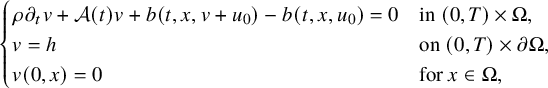 $$ \begin{align} \begin{cases} \rho\hspace{0.5pt} \partial_t v+\mathcal A(t) v+ b(t,x,v+u_0)-b(t,x,u_0)=0 & \mbox{in}\ (0,T)\times\Omega , \\ v=h &\mbox{on}\ (0,T)\times\partial\Omega,\\ v(0,x)=0 &\text{for } x\in\Omega, \end{cases} \end{align} $$
with $h:=f-f_0$
. Therefore, it is enough for our purpose to show that there exists
$h:=f-f_0$
. Therefore, it is enough for our purpose to show that there exists $\epsilon>0$
depending on a,
$\epsilon>0$
depending on a, $\rho $
, b,
$\rho $
, b, $f_0$
,
$f_0$
, $\Omega $
, T, such that for
$\Omega $
, T, such that for $h\in \mathbb B(0,\epsilon )$
, the problem (3.2) admits a unique solution
$h\in \mathbb B(0,\epsilon )$
, the problem (3.2) admits a unique solution $v_h\in C^{1+\frac {\alpha }{2},2+\alpha }([0,T]\times \overline {\Omega })$
satisfying
$v_h\in C^{1+\frac {\alpha }{2},2+\alpha }([0,T]\times \overline {\Omega })$
satisfying
 $$ \begin{align} \left\lVert v_h\right\rVert_{C^{1+\frac{\alpha}{2},2+\alpha}([0,T]\times\overline{\Omega})}\leqslant C\left\lVert h\right\rVert_{C^{1+\frac{\alpha}{2},2+\alpha}([0,T]\times\partial\Omega)}. \end{align} $$
We introduce the spaces
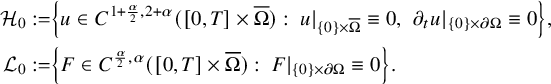 $$ \begin{align*} \begin{aligned} \mathcal H_0:=&\left\{u\in C^{1+\frac{\alpha}{2},2+\alpha}([0,T]\times\overline{\Omega}):\ u|_{\{0\}\times\overline{\Omega}}\equiv 0,\ \left. \partial_tu\right|{}_{\{0\}\times\partial\Omega}\equiv 0\right\}, \\ \mathcal L_0:=&\left\{F\in C^{\frac{\alpha}{2},\alpha}([0,T]\times\overline{\Omega}):\ F|_{\{0\}\times\partial\Omega}\equiv 0\right\}. \end{aligned} \end{align*} $$
Then, let us introduce the map $\mathcal G$
defined by
$\mathcal G$
defined by
 $$ \begin{align*} \mathcal G:\mathcal K_0\times\mathcal H_0 &\to \mathcal L_0\times\mathcal K_0 ,\\ (h,v) &\mapsto\left(\rho \hspace{0.5pt}\partial_t v+\mathcal A(t) v+ b(t,x,v+u_0)-b(t,x,u_0), \, v|_{\Sigma}-h\right). \end{align*} $$
We will find a solution to (1.2) by applying the implicit function theorem to the map $\mathcal G$
. Using the fact that
$\mathcal G$
. Using the fact that $b\in C^\infty ({\mathbb R};C^{\frac {\alpha }{2},\alpha }([0,T]\times \overline {\Omega }))$
, it follows that the map
$b\in C^\infty ({\mathbb R};C^{\frac {\alpha }{2},\alpha }([0,T]\times \overline {\Omega }))$
, it follows that the map $\mathcal G$
is
$\mathcal G$
is $C^\infty $
on
$C^\infty $
on $\mathcal K_0\times \mathcal H_0$
in the Fréchet sense. Moreover, we have
$\mathcal K_0\times \mathcal H_0$
in the Fréchet sense. Moreover, we have $\mathcal G(0,0)=(0,0)$
and
$\mathcal G(0,0)=(0,0)$
and
 $$ \begin{align*}\partial_v\mathcal G(0,0)w=\left(\rho\hspace{0.5pt} \partial_t w+\mathcal A(t) w+ \partial_\mu b(t,x,u_0)w, \, w|_{\Sigma}\right).\end{align*} $$
In order to apply the implicit function theorem, we will prove that the map $\partial _v\mathcal G(0,0)$
is an isomorphism from
$\partial _v\mathcal G(0,0)$
is an isomorphism from $\mathcal H_0$
to
$\mathcal H_0$
to $\mathcal L_0\times \mathcal K_0$
. For this purpose, let us fix
$\mathcal L_0\times \mathcal K_0$
. For this purpose, let us fix $(F,h)\in \mathcal L_0\times \mathcal K_0$
, and let us consider the linear parabolic problem
$(F,h)\in \mathcal L_0\times \mathcal K_0$
, and let us consider the linear parabolic problem
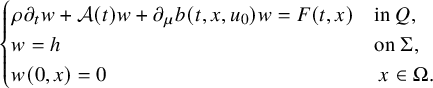 $$ \begin{align} \begin{cases} \rho \partial_t w+\mathcal A(t) w+ \partial_\mu b(t,x,u_0)w=F(t,x) & \mbox{in}\ Q , \\ w=h &\mbox{on}\ \Sigma,\\ w(0,x)=0 &\ x\in\Omega. \end{cases} \end{align} $$
Applying [Reference Ladyženskaja, Solonnikov and Ural’cevaLSU88, Theorem 5.2, Chapter IV, page 320], we deduce that problem (3.4) admits a unique solution $w\in \mathcal H_0$
satisfying
$w\in \mathcal H_0$
satisfying
 $$ \begin{align*}\left\lVert w\right\rVert_{C^{1+\frac{\alpha}{2},2+\alpha}([0,T]\times\overline{\Omega})}\leqslant C\left(\left\lVert F\right\rVert_{C^{\frac{\alpha}{2},\alpha}([0,T]\times\overline{\Omega})}+\left\lVert h\right\rVert_{C^{1+\frac{\alpha}{2},2+\alpha}([0,T]\times\partial\Omega)}\right),\end{align*} $$
for some constant $C>0$
independent of w, F and h. From this result, we deduce that
$C>0$
independent of w, F and h. From this result, we deduce that $\partial _v\mathcal G(0,0)$
is an isomorphism from
$\partial _v\mathcal G(0,0)$
is an isomorphism from $\mathcal H_0$
to
$\mathcal H_0$
to $\mathcal L_0\times \mathcal K_0$
.
$\mathcal L_0\times \mathcal K_0$
.
Therefore, applying the implicit function theorem (see, for example, [Reference Renardy and RogersRR06, Theorem 10.6]), we deduce that there exists $\epsilon>0$
depending on a, b,
$\epsilon>0$
depending on a, b, $\rho $
,
$\rho $
, $f_0$
,
$f_0$
, $\Omega $
, T, and a smooth map
$\Omega $
, T, and a smooth map $\psi $
from
$\psi $
from $\mathbb B(0,\epsilon )$
to
$\mathbb B(0,\epsilon )$
to $\mathcal H_0$
, such that, for all
$\mathcal H_0$
, such that, for all $h\in \mathbb B(0,\epsilon )$
, we have
$h\in \mathbb B(0,\epsilon )$
, we have $\mathcal G(h,\psi (h))=(0,0)$
. This proves that
$\mathcal G(h,\psi (h))=(0,0)$
. This proves that $v=\psi (h)$
is a solution of (3.2) for all
$v=\psi (h)$
is a solution of (3.2) for all $h\in \mathbb B(0,\epsilon )$
.
$h\in \mathbb B(0,\epsilon )$
.
For the uniqueness of the solution of (3.2), let us consider $v_1 \in C^{1+\frac {\alpha }{2},2+\alpha }([0,T]\times \overline {\Omega })$
to be a solution of (3.2), and let us show that
$v_1 \in C^{1+\frac {\alpha }{2},2+\alpha }([0,T]\times \overline {\Omega })$
to be a solution of (3.2), and let us show that $v_1=v$
. For this purpose, we fix
$v_1=v$
. For this purpose, we fix $w=v_1-v$
and notice that w solves the following initial boundary value problem
$w=v_1-v$
and notice that w solves the following initial boundary value problem
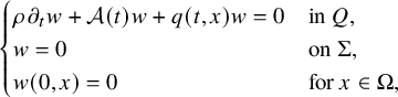 $$ \begin{align} \begin{cases} \rho\hspace{0.5pt} \partial_t w+\mathcal A(t) w+ q(t,x)w=0 & \mbox{in}\ Q , \\ w=0 &\mbox{on}\ \Sigma,\\ w(0,x)=0 &\text{for } x\in\Omega, \end{cases} \end{align} $$
with
 $$ \begin{align*}q(t,x)=\int_0^1\partial_\mu b(t,x,sv_1(t,x)+(1-s)v(t,x)+u_0(t,x))\, ds,\quad (t,x)\in Q.\end{align*} $$
Then the uniqueness of the solutions of (3.5) implies that $w\equiv 0$
, and by the same way that
$w\equiv 0$
, and by the same way that $v=v_1$
. Therefore,
$v=v_1$
. Therefore, $v=\psi (h)$
is the unique solution of (3.2). Combining this with the fact that
$v=\psi (h)$
is the unique solution of (3.2). Combining this with the fact that $\psi $
is smooth from
$\psi $
is smooth from $\mathbb B(0,\epsilon )$
to
$\mathbb B(0,\epsilon )$
to $\mathcal H_0$
and
$\mathcal H_0$
and $\psi (0)=0$
, we obtain (3.1). Finally, recalling that, for all
$\psi (0)=0$
, we obtain (3.1). Finally, recalling that, for all $f\in \mathbb B(f_0,\epsilon )$
,
$f\in \mathbb B(f_0,\epsilon )$
, $u_f=u_0+\psi (f-f_0)$
with
$u_f=u_0+\psi (f-f_0)$
with $\psi $
a
$\psi $
a $C^\infty $
map from
$C^\infty $
map from $\mathbb B(0,\epsilon )$
to
$\mathbb B(0,\epsilon )$
to $C^{1+\frac {\alpha }{2},2+\alpha }([0,T]\times \overline {\Omega }))$
, we deduce that the map
$C^{1+\frac {\alpha }{2},2+\alpha }([0,T]\times \overline {\Omega }))$
, we deduce that the map $\mathbb B(f_0,\epsilon )\ni f\mapsto u_f\in C^{1+\frac {\alpha }{2},2+\alpha }([0,T]\times \overline {\Omega }))$
is
$\mathbb B(f_0,\epsilon )\ni f\mapsto u_f\in C^{1+\frac {\alpha }{2},2+\alpha }([0,T]\times \overline {\Omega }))$
is $C^\infty $
. This completes the proof of the proposition.
$C^\infty $
. This completes the proof of the proposition.
3.2 Linearizations of the problem
In this subsection, we assume that the conditions of Proposition 3.1 are fulfilled. Let us introduce $m\in \mathbb N\cup \{0\}$
and consider the parameter
$m\in \mathbb N\cup \{0\}$
and consider the parameter $s=(s_1,\ldots ,s_{m+1})\in (-1,1)^{m+1}$
. Fixing
$s=(s_1,\ldots ,s_{m+1})\in (-1,1)^{m+1}$
. Fixing $h_1,\ldots ,h_{m+1}\in \mathbb B(0,\frac {\epsilon }{m+1})$
, we consider
$h_1,\ldots ,h_{m+1}\in \mathbb B(0,\frac {\epsilon }{m+1})$
, we consider $u=u_{s}$
the solution of
$u=u_{s}$
the solution of
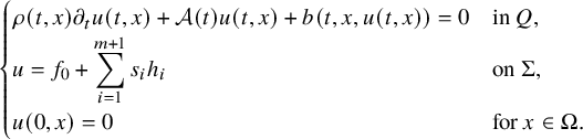 $$ \begin{align} \begin{cases} \rho(t,x) \partial_t u(t,x)+\mathcal A(t) u(t,x)+ b(t,x,u(t,x))=0 & \mbox{in}\ Q , \\ u=f_0+\displaystyle\sum_{i=1}^{m+1}s_ih_i &\mbox{on}\ \Sigma,\\ u(0,x)=0 &\text{for } x\in\Omega. \end{cases} \end{align} $$
Following the proof of Proposition 3.1, we know that the map $s\mapsto u_s$
is lying in
$s\mapsto u_s$
is lying in
 $$ \begin{align*}C^\infty\left((-1,1)^{m+1};C^{1+\frac{\alpha}{2},2+\alpha}([0,T]\times\overline{\Omega})\right).\end{align*} $$
Then we are able to differentiate (3.6) with respect to the s parameter.
Let us introduce the solution of the first linearized problem
 $$ \begin{align} \begin{cases} \rho(t,x) \partial_t v+\mathcal A(t) v+ \partial_\mu b(t,x,u_0)v=0 & \mbox{in}\ Q , \\ v=h &\mbox{on}\ \Sigma,\\ v(0,x)=0 &\text{for } x\in\Omega. \end{cases} \end{align} $$
Using the facts that $u_s|_{s=0}=u_0$
and that the map
$u_s|_{s=0}=u_0$
and that the map $s\mapsto u_s$
is smooth, we see that if
$s\mapsto u_s$
is smooth, we see that if $v_{\ell }$
is the solution of (3.7) with
$v_{\ell }$
is the solution of (3.7) with $h=h_\ell $
,
$h=h_\ell $
, $\ell =1,\ldots ,m+1$
, then we have
$\ell =1,\ldots ,m+1$
, then we have
 $$ \begin{align} \left.\partial_{s_\ell}u_{s}\right|{}_{s=0}= v_{\ell},\quad \ell=1,\ldots,m+1, \end{align} $$
in the sense of functions taking values in $C^{1+\frac {\alpha }{2},2+\alpha }([0,T]\times \overline {\Omega })$
.
$C^{1+\frac {\alpha }{2},2+\alpha }([0,T]\times \overline {\Omega })$
.
Now let us turn to the expression $\partial _{s_{\ell _1}}\partial _{s_{\ell _2}}u_{s}\big |_{s=0}$
,
$\partial _{s_{\ell _1}}\partial _{s_{\ell _2}}u_{s}\big |_{s=0}$
, $\ell _1,\ell _2=1,\ldots ,m+1$
. For this purpose, we introduce the function
$\ell _1,\ell _2=1,\ldots ,m+1$
. For this purpose, we introduce the function $w_{\ell _1,\ell _2}\in C^{1+\frac {\alpha }{2},2+\alpha }([0,T]\times \overline {\Omega })$
solving the second linearized problem
$w_{\ell _1,\ell _2}\in C^{1+\frac {\alpha }{2},2+\alpha }([0,T]\times \overline {\Omega })$
solving the second linearized problem
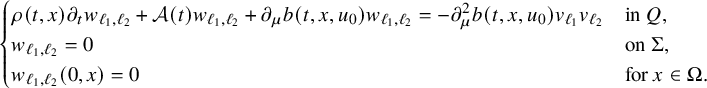 $$ \begin{align} \begin{cases} \rho(t,x) \partial_t w_{\ell_1,\ell_2}+\mathcal A(t) w_{\ell_1,\ell_2}+ \partial_\mu b(t,x,u_0) w_{\ell_1,\ell_2}=-\partial_\mu^2 b(t,x,u_0)v_{\ell_1}v_{\ell_2} & \mbox{in}\ Q, \\ w_{\ell_1,\ell_2}=0 &\mbox{on}\ \Sigma,\\ w_{\ell_1,\ell_2}(0,x)=0 &\text{for } x\in\Omega. \end{cases} \end{align} $$
Repeating the above arguments, we obtain that
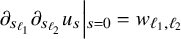 $$ \begin{align} \left. \partial_{s_{\ell_1}}\partial_{s_{\ell_2}}u_{s}\right|{}_{s=0}= w_{\ell_1,\ell_2} \end{align} $$
is the solution to (3.9). Then, by iterating the above arguments, one has the following result.
Lemma 3.1 (Higher-order linearizations).
Let $m\in \mathbb N$
. The function
$m\in \mathbb N$
. The function
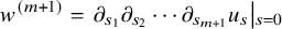 $$ \begin{align} w^{(m+1)}=\left.\partial_{s_1}\partial_{s_2}\cdots\partial_{s_{m+1}}u_{s}\right|{}_{s=0} \end{align} $$
is well defined in the sense of functions taking values in $C^{1+\frac {\alpha }{2},2+\alpha }([0,T]\times \overline {\Omega })$
. Moreover,
$C^{1+\frac {\alpha }{2},2+\alpha }([0,T]\times \overline {\Omega })$
. Moreover, $w^{(m+1)}$
solves the
$w^{(m+1)}$
solves the $(m+1)$
-th order linearized problem
$(m+1)$
-th order linearized problem
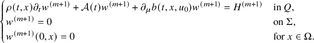 $$ \begin{align} \begin{cases} \rho(t,x) \partial_t w^{(m+1)}+\mathcal A(t) w^{(m+1)}+ \partial_\mu b(t,x,u_0) w^{(m+1)}=H^{(m+1)} & \mbox{in}\ Q, \\ w^{(m+1)}=0 &\mbox{on}\ \Sigma,\\ w^{(m+1)}(0,x)=0 &\mbox{for } x\in\Omega. \end{cases} \end{align} $$
Here, we have
 $$ \begin{align} H^{(m+1)}=-\partial_\mu^{m+1} b(t,x,u_0)v_{1}\cdots v_{m+1} +K^{(m+1)}, \end{align} $$
where all the functions are evaluated at the point $(t,x)$
and
$(t,x)$
and $K^{(m+1)}(t,x)$
depends only on a,
$K^{(m+1)}(t,x)$
depends only on a, $\rho $
,
$\rho $
, $\Omega $
, T,
$\Omega $
, T, $\partial _\mu ^k b(t,x,u_0)$
,
$\partial _\mu ^k b(t,x,u_0)$
, $k=0,\ldots ,m$
,
$k=0,\ldots ,m$
, $v_1,\ldots , v_{m+1}$
, and
$v_1,\ldots , v_{m+1}$
, and $w^{(k+1)}$
, for
$w^{(k+1)}$
, for $k=1,\ldots , m-1$
. Here,
$k=1,\ldots , m-1$
. Here, $v_1,\ldots , v_{m+1}$
are the solutions of (3.7) with
$v_1,\ldots , v_{m+1}$
are the solutions of (3.7) with $h=h_\ell $
,
$h=h_\ell $
, $\ell =1,\ldots ,m+1$
.
$\ell =1,\ldots ,m+1$
.
4 Proof of Theorem 2.1
In this section, we will prove Theorem 2.1 by admitting the proof of the following denseness result.
Proposition 4.1. Adopting all the conditions of Theorem 2.1, consider $F\in C([0,T]\times \overline {\Omega })$
,
$F\in C([0,T]\times \overline {\Omega })$
, $m\in \mathbb N$
and
$m\in \mathbb N$
and $q_0,\ldots ,q_m\in C^{\frac {\alpha }{2},\alpha }([0,T]\times \overline {\Omega })$
. Assume that the identity
$q_0,\ldots ,q_m\in C^{\frac {\alpha }{2},\alpha }([0,T]\times \overline {\Omega })$
. Assume that the identity
 $$ \begin{align} \int_0^T\int_\Omega Fv_1\cdots v_m\hspace{0.5pt} w \, dxdt=0 \end{align} $$
holds true for all $v_j\in C^{1+\frac {\alpha }{2},2+\alpha }([0,T]\times \overline {\Omega }))$
and
$v_j\in C^{1+\frac {\alpha }{2},2+\alpha }([0,T]\times \overline {\Omega }))$
and $w\in C^{1+\frac {\alpha }{2},2+\alpha }([0,T]\times \overline {\Omega }))$
solving the following equations
$w\in C^{1+\frac {\alpha }{2},2+\alpha }([0,T]\times \overline {\Omega }))$
solving the following equations
 $$ \begin{align} \begin{cases} \rho(t,x) \partial_t v_j+\mathcal A(t) v_j+ {q_j}v_j=0, & \mbox{in}\ Q ,\\ v_j(0,x)=0 &\mbox{for } x\in\Omega, \end{cases} \end{align} $$
for $j=1,\ldots , m$
, and
$j=1,\ldots , m$
, and
 $$ \begin{align} \begin{cases} -\partial_t(\rho(t,x) w)+\mathcal A(t) w+ {q_0}w=0, & \mbox{in}\ Q , \\ w(T,x)=0 &\mbox{for } x\in\Omega, \end{cases} \end{align} $$
respectively. Then $F\equiv 0$
.
$F\equiv 0$
.
We next use the above proposition to show Theorem 2.1. The proof of the proposition will be postponed to Section 5.
Proof of Theorem 2.1.
We will prove this theorem in two steps. We will start by proving that the assumption
 $$ \begin{align*} \mathcal N_{b_1}(f)=\mathcal N_{b_2}(f), \text{ for all }f\in \mathbb B(f_0,\epsilon) \end{align*} $$
implies that
 $$ \begin{align} \partial_\mu^k b_1\left(t,x,u_{1,0}(t,x)\right)=\partial_\mu^k b_2\left(t,x,u_{2,0}(t,x)\right),\quad (t,x)\in [0,T]\times\overline{\Omega} \end{align} $$
holds true for all $k\in \mathbb N$
, with
$k\in \mathbb N$
, with $u_{j,0}$
being the solution of (1.2) with
$u_{j,0}$
being the solution of (1.2) with $b=b_j$
and
$b=b_j$
and $f=f_0$
, for
$f=f_0$
, for $j=1,2$
. Then we will complete the proof by showing that (4.4) implies the claim
$j=1,2$
. Then we will complete the proof by showing that (4.4) implies the claim
 $$ \begin{align*} b_1=S_\varphi b_2 \end{align*} $$
for some $\varphi \in C^{1+\frac {\alpha }{2},2+\alpha }([0,T]\times \overline {\Omega })$
satisfying the condition (1.6).
$\varphi \in C^{1+\frac {\alpha }{2},2+\alpha }([0,T]\times \overline {\Omega })$
satisfying the condition (1.6).
Step 1. Determination of the Taylor coefficients
We will show (4.4) holds true, for all $k\in \mathbb N$
, by recursion. Note first that, for
$k\in \mathbb N$
, by recursion. Note first that, for $j=1,2$
, the function
$j=1,2$
, the function $(t,x) \mapsto \partial _\mu b_j(t,x,u_{j,0}(t,x))$
belongs to
$(t,x) \mapsto \partial _\mu b_j(t,x,u_{j,0}(t,x))$
belongs to $ C^{\frac {\alpha }{2},\alpha }([0,T]\times \overline {\Omega })$
. Thus, for
$ C^{\frac {\alpha }{2},\alpha }([0,T]\times \overline {\Omega })$
. Thus, for $j=1,2$
, we can consider
$j=1,2$
, we can consider $v_{j,1}\in C^{1+\frac {\alpha }{2},2+\alpha }([0,T]\times \overline {\Omega }))$
satisfying (4.2) with
$v_{j,1}\in C^{1+\frac {\alpha }{2},2+\alpha }([0,T]\times \overline {\Omega }))$
satisfying (4.2) with $q_j(t,x)=\partial _\mu b_j(t,x,u_{j,0}(t,x))$
and
$q_j(t,x)=\partial _\mu b_j(t,x,u_{j,0}(t,x))$
and $w\in C^{1+\frac {\alpha }{2},2+\alpha }([0,T]\times \overline {\Omega }))$
satisfying (4.3) with
$w\in C^{1+\frac {\alpha }{2},2+\alpha }([0,T]\times \overline {\Omega }))$
satisfying (4.3) with $q_0(t,x)=\partial _\mu b_1(t,x,u_{1,0}(t,x))$
. We assume here that
$q_0(t,x)=\partial _\mu b_1(t,x,u_{1,0}(t,x))$
. We assume here that $\left. v_{1,1}\right |{}_{\Sigma }=h=\left. v_{2,1}\right |{}_{\Sigma }$
for some
$\left. v_{1,1}\right |{}_{\Sigma }=h=\left. v_{2,1}\right |{}_{\Sigma }$
for some $h\in \mathbb B(0,1)$
. Applying the first-order linearization, we find
$h\in \mathbb B(0,1)$
. Applying the first-order linearization, we find
 $$ \begin{align*}\left. \partial_{\nu(a)} v_{1,1}\right|{}_{\Sigma}=\partial_s\mathcal N_{b_1}(f_0+sh)=\partial_s\mathcal N_{b_2}(f_0+sh)=\left.\partial_{\nu(a)} v_{2,1}\right|{}_{\Sigma}.\end{align*} $$
Thus, fixing $v_1=v_{1,1}-v_{2,1}$
, we deduce that
$v_1=v_{1,1}-v_{2,1}$
, we deduce that $v_1$
satisfies the conditions
$v_1$
satisfies the conditions
 $$ \begin{align} \begin{cases} \rho(t,x) \partial_t v_1+\mathcal A(t) v_1+ \partial_\mu b_1(t,x,{u_{1,0}(t,x)})v_1 =G(t,x) & \mbox{in}\ Q , \\ v_1=\partial_{\nu_a}v_1=0 &\mbox{on}\ \Sigma,\\ v(0,x)=0 &\mbox{for } x\in\Omega, \end{cases} \end{align} $$
where
 $$ \begin{align*}G(t,x)=\left(\partial_\mu b_2(t,x,u_{2,0}(t,x))-\partial_\mu b_1(t,x,u_{1,0}(t,x))\right)v_{2,1}(t,x),\quad (t,x)\in Q. \end{align*} $$
Multiplying the equation (4.5) by w and integrating by parts, we obtain the identity
 $$ \begin{align*} \begin{aligned} &\quad \, \int_0^T\int_{\Omega}\left(\partial_\mu b_2(t,x,u_{2,0})-\partial_\mu b_1(t,x,u_{1,0})\right)v_{2,1}w \, dx dt \\ &= \int_{0}^{T}\int_{\Omega} \left( \rho(t,x) \partial_t v_1+\mathcal A(t) v_1+ \partial_\mu b_1(t,x,{u_{1,0}(t,x)})v_1\right) w\, dxdt \\ &=\underbrace{\int_{0}^{T}\int_{\Omega} \left( -\partial_t (\rho w) +\mathcal{A}(t)w+ \partial_\mu b_1(t,x,{u_{1,0}(t,x)})w \right) v_1 \, dxdt}_{\text{Since } v_1=\partial_{\nu(a)} v_1 =0 \text{ on }\Sigma, \ v_1(0,x)=0 \text{ and } w(T,x)=0 \text{ in } \Omega.} \\ &= 0. \end{aligned} \end{align*} $$
Using the the fact that $v_{2,1}$
can be seen as an arbitrary chosen element of
$v_{2,1}$
can be seen as an arbitrary chosen element of $C^{1+\frac {\alpha }{2},2+\alpha }([0,T]\times \overline {\Omega }))$
satisfying (4.2) and applying Proposition 4.1, we deduce that (4.4) holds true for
$C^{1+\frac {\alpha }{2},2+\alpha }([0,T]\times \overline {\Omega }))$
satisfying (4.2) and applying Proposition 4.1, we deduce that (4.4) holds true for $k=1$
. Moreover, by the unique solvability of (3.7), we deduce that
$k=1$
. Moreover, by the unique solvability of (3.7), we deduce that $v_{1,1}=v_{2,1}$
in Q.
$v_{1,1}=v_{2,1}$
in Q.
Now, let us fix $m\in \mathbb N$
and assume that, for
$m\in \mathbb N$
and assume that, for $k=1,\ldots ,m$
, (4.4) holds true and
$k=1,\ldots ,m$
, (4.4) holds true and
 $$ \begin{align} w_1^{(k)}=w_2^{(k)} \text{ in } Q. \end{align} $$
Consider $v_j\in C^{1+\frac {\alpha }{2},2+\alpha }([0,T]\times \overline {\Omega }))$
satisfying (4.2) with
$v_j\in C^{1+\frac {\alpha }{2},2+\alpha }([0,T]\times \overline {\Omega }))$
satisfying (4.2) with $q_j(t,x)=\partial _\mu b_1(t,x,u_{1,0}(t,x))$
for
$q_j(t,x)=\partial _\mu b_1(t,x,u_{1,0}(t,x))$
for $j=1,\ldots , m+1$
, and
$j=1,\ldots , m+1$
, and $w\in C^{1+\frac {\alpha }{2},2+\alpha }([0,T]\times \overline {\Omega }))$
satisfying (4.2) with
$w\in C^{1+\frac {\alpha }{2},2+\alpha }([0,T]\times \overline {\Omega }))$
satisfying (4.2) with $q_0(t,x)=\partial _\mu b_1(t,x,u_{1,0}(t,x))$
. We fix
$q_0(t,x)=\partial _\mu b_1(t,x,u_{1,0}(t,x))$
. We fix $h_j=\left. v_j\right |{}_{\Sigma }$
,
$h_j=\left. v_j\right |{}_{\Sigma }$
, $j=1,\ldots ,m+1$
, and proceeding to the higher-order linearization described in Lemma 3.1, we obtain
$j=1,\ldots ,m+1$
, and proceeding to the higher-order linearization described in Lemma 3.1, we obtain
 $$ \begin{align*}\left.\partial_{\nu(a)} w^{(m+1)}_j\right|{}_{\Sigma}=\left.\partial_{s_{1}}\ldots\partial_{s_{m+1}}\mathcal N_{b_j}(f_0+s_1h_1+\ldots+s_{m+1}h_{m+1})\right|{}_{s=0},\end{align*} $$
with $s=(s_1,\ldots ,s_{m+1})$
and
$s=(s_1,\ldots ,s_{m+1})$
and $w^{(m+1)}_j$
solving (3.12) as
$w^{(m+1)}_j$
solving (3.12) as $b=b_j$
, for
$b=b_j$
, for $j=1,2$
. Then the condition (2.4) implies
$j=1,2$
. Then the condition (2.4) implies
 $$ \begin{align*}\left.\partial_{\nu(a)} w^{(m+1)}_1\right|{}_{\Sigma}=\left.\partial_{\nu(a)} w^{(m+1)}_2\right|{}_{\Sigma}.\end{align*} $$
Fixing $w^{(m+1)}=w^{(m+1)}_1-w^{(m+1)}_2$
and applying Lemma 3.1, we deduce that
$w^{(m+1)}=w^{(m+1)}_1-w^{(m+1)}_2$
and applying Lemma 3.1, we deduce that $w^{(m+1)}$
satisfies the condition
$w^{(m+1)}$
satisfies the condition
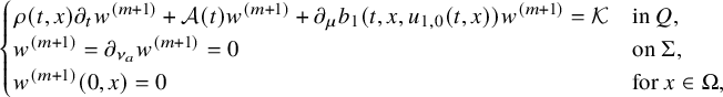 $$ \begin{align} \begin{cases} \rho(t,x) \partial_t w^{(m+1)}+\mathcal A(t) w^{(m+1)}+ \partial_\mu b_1(t,x,{u_{1,0}(t,x)}) w^{(m+1)}=\mathcal K & \mbox{in}\ Q, \\ w^{(m+1)}=\partial_{\nu_a} w^{(m+1)}=0 &\mbox{on}\ \Sigma,\\ w^{(m+1)}(0,x)=0 &\mbox{for } x\in\Omega, \end{cases} \end{align} $$
where $\mathcal K= (\partial _\mu ^{m+1} b_2(t,x,u_{2,0})-\partial _\mu ^{m+1} b_1(t,x,u_{1,0}) )v_1\cdots v_{m+1}$
. Here, we used the assumption for this recursion argument that (4.4) and (4.6) hold true for
$\mathcal K= (\partial _\mu ^{m+1} b_2(t,x,u_{2,0})-\partial _\mu ^{m+1} b_1(t,x,u_{1,0}) )v_1\cdots v_{m+1}$
. Here, we used the assumption for this recursion argument that (4.4) and (4.6) hold true for $k=1,\ldots ,m$
. Multiplying the equation (4.7) by w and integrating by parts, we obtain
$k=1,\ldots ,m$
. Multiplying the equation (4.7) by w and integrating by parts, we obtain
 $$ \begin{align*}\int_0^T\int_\Omega \left(\partial_\mu^{m+1} b_2(t,x,u_{2,0})-\partial_\mu^{m+1} b_1(t,x,u_{1,0})\right)v_1\cdots v_{m+1}\hspace{0.5pt} w\, dxdt=0.\end{align*} $$
Applying again Proposition 4.1, we find that (4.4) holds true for $k=1,\ldots ,m+1$
. By unique solvability of (3.7), we also have
$k=1,\ldots ,m+1$
. By unique solvability of (3.7), we also have $w_1^{(m+1)}=w_2^{(m+1)}$
in Q. It follows that (4.4) holds true for all
$w_1^{(m+1)}=w_2^{(m+1)}$
in Q. It follows that (4.4) holds true for all $k\in \mathbb N$
.
$k\in \mathbb N$
.
Step 2. Gauge invariance.
In this step, we will show that (2.5) holds with some $\varphi \in C^{1+\frac {\alpha }{2},2+\alpha }([0,T]\times \overline {\Omega })$
satisfying (1.6). We will choose here
$\varphi \in C^{1+\frac {\alpha }{2},2+\alpha }([0,T]\times \overline {\Omega })$
satisfying (1.6). We will choose here $\varphi =u_{2,0}-u_{1,0}$
and, thanks to (2.4), we know that
$\varphi =u_{2,0}-u_{1,0}$
and, thanks to (2.4), we know that $\varphi $
fulfills condition (1.6). We fix
$\varphi $
fulfills condition (1.6). We fix $(t,x)\in [0,T]\times \overline {\Omega }$
and consider the map
$(t,x)\in [0,T]\times \overline {\Omega }$
and consider the map
 $$ \begin{align*}G_j:{\mathbb R}\ni\mu\mapsto b_j(t,x,u_{j,0}(t,x)+\mu)-b_j(t,x,u_{j,0}(t,x)),\quad j=1,2.\end{align*} $$
For $j=1,2$
, using the fact that
$j=1,2$
, using the fact that $b_j\in \mathbb A({\mathbb R};C^{\frac {\alpha }{2},\alpha }([0,T]\times \overline {\Omega }))$
, we deduce that the map
$b_j\in \mathbb A({\mathbb R};C^{\frac {\alpha }{2},\alpha }([0,T]\times \overline {\Omega }))$
, we deduce that the map $G=G_1-G_2$
is analytic with respect to
$G=G_1-G_2$
is analytic with respect to $\mu \in {\mathbb R}$
. It is clear that
$\mu \in {\mathbb R}$
. It is clear that
 $$ \begin{align*}G(0)=G_1(0)-G_2(0)=0-0=0. \end{align*} $$
Moreover, (4.4) implies that
 $$ \begin{align*}G^{(k)}(0)=\partial_\mu^kb_1(t,x,u_{1,0}(t,x))-\partial_\mu^kb_2(t,x,u_{2,0}(t,x))=0,\quad k\in\mathbb N.\end{align*} $$
Combining this with the fact that G is analytic with respect to $\mu \in {\mathbb R}$
, we deduce that there must exist
$\mu \in {\mathbb R}$
, we deduce that there must exist $\delta>0$
such that
$\delta>0$
such that
 $$ \begin{align*}G(\mu)=0,\quad \mu\in(-\delta,\delta).\end{align*} $$
Then, the unique continuation of analytic functions implies that $G\equiv 0$
. It follows that, for all
$G\equiv 0$
. It follows that, for all $\mu \in {\mathbb R}$
, we have
$\mu \in {\mathbb R}$
, we have
 $$ \begin{align*}b_1(t,x,u_{1,0}(t,x)+\mu)-b_1(t,x,u_{1,0}(t,x))=b_2(t,x,u_{2,0}(t,x)+\mu)-b_2(t,x,u_{2,0}(t,x)).\end{align*} $$
Recalling that
 $$ \begin{align*}-b_j(t,x,u_{j,0}(t,x))=\rho(t,x) \partial_t u_{j,0}(t,x)+\mathcal A(t)u_{j,0}(t,x),\quad j=1,2,\end{align*} $$
we deduce that
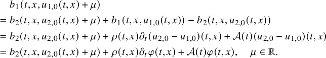 $$ \begin{align} \begin{aligned} &\quad \, b_1(t,x,u_{1,0}(t,x)+\mu)\\ &=b_2(t,x,u_{2,0}(t,x)+\mu)+b_1(t,x,u_{1,0}(t,x))-b_2(t,x,u_{2,0}(t,x))\\ &=b_2(t,x,u_{2,0}(t,x)+\mu)+\rho(t,x) \partial_t(u_{2,0}-u_{1,0})(t,x)+\mathcal A(t)(u_{2,0}-u_{1,0})(t,x)\\ &=b_2(t,x,u_{2,0}(t,x)+\mu)+\rho(t,x) \partial_t \varphi(t,x)+\mathcal A(t)\varphi(t,x),\quad \mu\in{\mathbb R}. \end{aligned} \end{align} $$
Considering (4.8) with $\mu _1=u_{1,0}(t,x)+\mu $
, we obtain
$\mu _1=u_{1,0}(t,x)+\mu $
, we obtain
 $$ \begin{align*}\begin{aligned}b_1(t,x,\mu_1)&=b_2(t,x,u_{2,0}(t,x)-u_{1,0}(t,x)+\mu_1)+\rho(t,x) \partial_t \varphi(t,x)+\mathcal A(t)\varphi(t,x)\\ &=b_2(t,x,\varphi(t,x)+\mu_1)+\rho(t,x) \partial_t \varphi(t,x)+\mathcal A(t)\varphi(t,x),\quad \mu_1\in{\mathbb R}.\end{aligned}\end{align*} $$
Using the fact that here $(t,x)\in [0,T]\times \overline {\Omega }$
is arbitrary chosen, we deduce that (2.5) holds true with
$(t,x)\in [0,T]\times \overline {\Omega }$
is arbitrary chosen, we deduce that (2.5) holds true with $\varphi =u_{2,0}-u_{1,0}$
. This completes the proof of the theorem.
$\varphi =u_{2,0}-u_{1,0}$
. This completes the proof of the theorem.
5 Proof of Proposition 4.1
In order to prove Proposition 4.1, we need to construct special solutions, which helps us to prove the completeness of products of solutions.
5.1 Constructions of geometric optics solutions
For the proof of Proposition 4.1, we will need to consider the construction of geometrical optics (GO in short) solutions. More precisely, fixing $q\in C^{\frac {\alpha }{2},\alpha }([0,T]\times \overline {\Omega })$
, we will consider GO solutions to the equation
$q\in C^{\frac {\alpha }{2},\alpha }([0,T]\times \overline {\Omega })$
, we will consider GO solutions to the equation
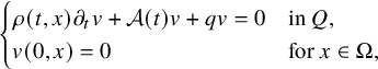 $$ \begin{align} \begin{cases} \rho(t,x)\partial_tv+\mathcal A(t) v+qv =0 & \mbox{in}\ Q , \\ v(0,x)=0 &\mbox{for } x\in\Omega, \end{cases} \end{align} $$
as well as GO solutions for the formal adjoint equation
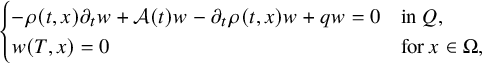 $$ \begin{align} \begin{cases} -\rho(t,x)\partial_tw+\mathcal A(t) w-\partial_t\rho(t,x)w+qw=0 & \mbox{in}\ Q , \\ w(T,x)=0 &\mbox{for } x\in\Omega, \end{cases} \end{align} $$
belonging to the space $C^{1+\frac {\alpha }{2},2+\alpha }([0,T]\times \overline {\Omega })$
. Following the recent construction of [Reference FeizmohammadiFei23], in this section, we give a construction of these GO solutions that will depend on a large asymptotic positive parameter
$C^{1+\frac {\alpha }{2},2+\alpha }([0,T]\times \overline {\Omega })$
. Following the recent construction of [Reference FeizmohammadiFei23], in this section, we give a construction of these GO solutions that will depend on a large asymptotic positive parameter $\tau $
with
$\tau $
with $\tau \gg 1$
and concentrate on geodesics with respect to the metric
$\tau \gg 1$
and concentrate on geodesics with respect to the metric $g(t)=\rho (t,\,\cdot \,)a(t,\,\cdot \,)^{-1}$
in
$g(t)=\rho (t,\,\cdot \,)a(t,\,\cdot \,)^{-1}$
in $\overline {\Omega _1}$
that passes through a point
$\overline {\Omega _1}$
that passes through a point $x_0\in \partial \Omega _1$
, whenever Assumption 2.1 holds. Here,
$x_0\in \partial \Omega _1$
, whenever Assumption 2.1 holds. Here, $\Omega _1$
is a domain satisfying Assumption 2.1 containing
$\Omega _1$
is a domain satisfying Assumption 2.1 containing $\overline {\Omega }$
. Let us construct the GO solution as follows.
$\overline {\Omega }$
. Let us construct the GO solution as follows.
First, we consider solutions of the form
 $$ \begin{align} v(t,x)=e^{\tau^2t+\tau \psi(t,x)}\left[c_{+}(t,x)+R_{+,\tau}(t,x)\right],\quad (t,x)\in Q, \end{align} $$
and
 $$ \begin{align} w(t,x)=e^{-\tau^2t-\tau \psi(t,x)}\left[c_{-}(t,x)+R_{-,\tau}(t,x)\right],\quad (t,x)\in Q, \end{align} $$
to equations (5.1) and (5.2), respectively. The phase functions and principal terms $c_\pm $
of the GOs will be constructed by using polar normal coordinate on the manifold
$c_\pm $
of the GOs will be constructed by using polar normal coordinate on the manifold $(\overline {\Omega _1}, g(t) )$
, for
$(\overline {\Omega _1}, g(t) )$
, for $t\in [0,T]$
.
$t\in [0,T]$
.
Let us define the differential operators $L_\pm $
,
$L_\pm $
, $P_{\tau ,\pm }$
on
$P_{\tau ,\pm }$
on $\Omega _1$
by
$\Omega _1$
by
 $$ \begin{align} \begin{aligned} L_{+}&=\rho(t,x)\partial_t+\mathcal A(t)+q(t,x),\\ L_{-}&=-\rho(t,x)\partial_t+\mathcal A(t) -\partial_t\rho(t,x)+q(t,x), \end{aligned} \end{align} $$
and
 $$ \begin{align} P_{\tau,\pm}= e^{\mp (\tau^2t+\tau \psi(t,x))}L_{\pm}\left( e^{\pm (\tau^2t+\tau \psi(t,x))} \right). \end{align} $$
Via a straightforward computation, we can write
 $$ \begin{align*}P_{\tau,\pm}v=\tau^2\, \mathcal I v+ \tau\, \mathcal J_{\pm}v + L_{\pm}v,\end{align*} $$
where
 $$ \begin{align} \mathcal I=\rho(t,x)-\sum_{i,k=1}^na_{ik}(t,x)\partial_{x_i}\psi\partial_{x_k}\psi, \end{align} $$
and
 $$ \begin{align} \mathcal J_\pm v:=\mp2\sum_{i,k=1}^na_{ik}(t,x)\partial_{x_i}\psi\partial_{x_k} v+\left[\rho(t,x)\partial_t \psi\pm\mathcal A(t)\psi\right]v. \end{align} $$
Next, we want to choose $\psi $
in such a way that the eikonal equation
$\psi $
in such a way that the eikonal equation $\mathcal I=0$
is satisfied in Q. Hence, after choosing
$\mathcal I=0$
is satisfied in Q. Hence, after choosing $\psi $
, we seek for
$\psi $
, we seek for $c_{\pm }$
solving the transport equations
$c_{\pm }$
solving the transport equations
 $$ \begin{align} \mathcal J_+c_{+}=0\quad \text{ and } \quad \mathcal J_-c_{-}=0. \end{align} $$
Since for all $t\in [0,T]$
, the Riemannian manifold
$t\in [0,T]$
, the Riemannian manifold $ (\overline {\Omega _1}, g(t) )$
is assumed to be simple, the eikonal equation
$ (\overline {\Omega _1}, g(t) )$
is assumed to be simple, the eikonal equation $\mathcal I=0$
can be solved globally on
$\mathcal I=0$
can be solved globally on $\overline {Q}$
. This is known, but let us show how it is done. For this, let us fix
$\overline {Q}$
. This is known, but let us show how it is done. For this, let us fix $x_0\in \partial \Omega _1$
and consider the polar normal coordinates
$x_0\in \partial \Omega _1$
and consider the polar normal coordinates $(r,\theta )$
on
$(r,\theta )$
on $ (\overline {\Omega _1}, g(t) )$
given by
$ (\overline {\Omega _1}, g(t) )$
given by $x=\exp _{x_0}(r\hspace {0.5pt} \theta )$
, where
$x=\exp _{x_0}(r\hspace {0.5pt} \theta )$
, where $r>0$
and
$r>0$
and
 $$ \begin{align*}\theta\in S_{x_0,t}(\overline{\Omega_1}):=\left\{v\in {\mathbb R}^n:\, |v|_{g(t)[x_0]}=1\right\}. \end{align*} $$
According to the Gauss lemma, in these coordinates, the metric takes the form
 $$ \begin{align*}dr^2+g_0(t,r,\theta), \end{align*} $$
where $g_0(t,r,\theta )$
is a metric defined on
$g_0(t,r,\theta )$
is a metric defined on $S_{x_0,t}(\overline {\Omega _1})$
, which depends smoothly on t and r. In fact, we choose
$S_{x_0,t}(\overline {\Omega _1})$
, which depends smoothly on t and r. In fact, we choose
 $$ \begin{align} \psi(t,x)=\textrm{dist}_{g(t)}(x_0,x), \quad (t,x) \in [0,T]\times\overline{\Omega}, \end{align} $$
where $\text {dist}_{g(t)}(\cdot ,\cdot ) $
is the Riemannian distance function associated with the metric
$\text {dist}_{g(t)}(\cdot ,\cdot ) $
is the Riemannian distance function associated with the metric $g(t)$
, for
$g(t)$
, for $t\in [0,T]$
. As
$t\in [0,T]$
. As $\psi $
is given by r in the polar normal coordinates, one can easily check that
$\psi $
is given by r in the polar normal coordinates, one can easily check that $\psi $
solves
$\psi $
solves $\mathcal I=0$
.
$\mathcal I=0$
.
Let us now turn to the transport equations (5.9). We write $c_{\pm }(t,r,\theta )=c_{\pm }(t,\exp _{x_0}(r\hspace {0.5pt} \theta ))$
and use this notation to indicate the representation in the polar normal coordinates also for other functions. Then, using this notation and following [Reference FeizmohammadiFei23, Section 5.1.2], we deduce that, in these polar normal coordinates with respect to
$c_{\pm }(t,r,\theta )=c_{\pm }(t,\exp _{x_0}(r\hspace {0.5pt} \theta ))$
and use this notation to indicate the representation in the polar normal coordinates also for other functions. Then, using this notation and following [Reference FeizmohammadiFei23, Section 5.1.2], we deduce that, in these polar normal coordinates with respect to $x_0\in \partial \Omega _1$
, the equations in (5.9) become
$x_0\in \partial \Omega _1$
, the equations in (5.9) become
 $$ \begin{align} \partial_rc_{\pm}+\left({\partial_r\beta \over 4\beta}\right)c_{\pm}\mp \frac{\partial_t\psi(t,r,\theta)}{2}c_{\pm}=0 \end{align} $$
with $\beta (t,r,\theta )=\det (g_0(t,r,\theta ) )$
. Note that in this equation, there is no differentiation in the
$\beta (t,r,\theta )=\det (g_0(t,r,\theta ) )$
. Note that in this equation, there is no differentiation in the $\theta $
-variable. This fact will allow us to localize GO solutions near geodesics. We fix
$\theta $
-variable. This fact will allow us to localize GO solutions near geodesics. We fix
 $$ \begin{align*}r_0=\inf_{t\in[0,T]}\textrm{dist}_{g(t)}(\partial\Omega_1,\overline{\Omega})\end{align*} $$
and recall that $r_0>0$
. For any
$r_0>0$
. For any $h\in C^\infty ( S_{x_0,t}(\overline {\Omega }_1))$
and
$h\in C^\infty ( S_{x_0,t}(\overline {\Omega }_1))$
and $\chi \in C^\infty _0(0,T)$
, the functions
$\chi \in C^\infty _0(0,T)$
, the functions
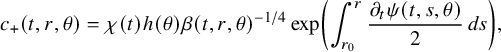 $$ \begin{align} &c_{+}(t,r,\theta)=\chi(t)h(\theta)\beta(t,r,\theta)^{-1/4}\exp\left( \int_{r_0}^{r}\frac{\partial_t\psi(t,s,\theta)}{2} \, ds\right), \end{align} $$
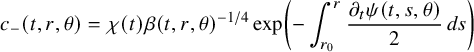 $$ \begin{align} &c_{-}(t,r,\theta)=\chi(t)\beta(t,r,\theta)^{-1/4}\exp\left( - \int_{r_0}^{r}\frac{\partial_t\psi(t,s,\theta)}{2}\, ds\right)\quad \ \end{align} $$
are respectively solutions of the transport equations (5.9). Moreover, the regularity of the coefficients $\rho $
, a and the simplicity of the manifold
$\rho $
, a and the simplicity of the manifold $ (\overline {\Omega _1}, g(t) )$
implies that solutions of the transport equation (5.11)
$ (\overline {\Omega _1}, g(t) )$
implies that solutions of the transport equation (5.11) $c_\pm \in C^\infty ([0,T]\times \overline {\Omega })$
.
$c_\pm \in C^\infty ([0,T]\times \overline {\Omega })$
.
In order to complete our construction of GO solutions, we need to show that it is possible to construct the remainder terms $R_{\pm ,\tau }\in C^{1+\frac {\alpha }{2},2+\alpha }([0,T]\times \overline {\Omega })$
satisfying the decay property
$R_{\pm ,\tau }\in C^{1+\frac {\alpha }{2},2+\alpha }([0,T]\times \overline {\Omega })$
satisfying the decay property
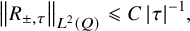 $$ \begin{align} \left\| R_{\pm,\tau}\right\|_{L^2(Q)}\leqslant C\,|\tau|^{-1}, \end{align} $$
for some constant $C>0$
independent of
$C>0$
independent of $\tau $
, positive and large enough, as well as the initial and final condition
$\tau $
, positive and large enough, as well as the initial and final condition
 $$ \begin{align*}R_{+,\tau}(0,x)=R_{-,\tau}(T,x)=0,\quad x\in\Omega.\end{align*} $$
For this purpose, we recall that for $\psi $
given by (5.10), we have
$\psi $
given by (5.10), we have $P_{\tau ,\pm }=L_{\pm }+\tau \mathcal J_\pm $
with
$P_{\tau ,\pm }=L_{\pm }+\tau \mathcal J_\pm $
with $L_\pm $
and
$L_\pm $
and $\mathcal J_\pm $
defined by (5.5)–(5.8). Then, according to (5.9), we have
$\mathcal J_\pm $
defined by (5.5)–(5.8). Then, according to (5.9), we have
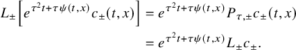 $$ \begin{align*}\begin{aligned}L_\pm\left[e^{\tau^2t+\tau \psi(t,x)}c_{\pm}(t,x)\right] &=e^{\tau^2t+\tau \psi(t,x)}P_{\tau,\pm}c_{\pm}(t,x)\\ &=e^{\tau^2t+\tau \psi(t,x)}L_{\pm}c_{\pm}.\end{aligned}\end{align*} $$
Therefore, the conditions $L_{+}v=0$
and
$L_{+}v=0$
and $L_-w=0$
are fulfilled if and only if
$L_-w=0$
are fulfilled if and only if $R_{\pm ,\tau }$
solves
$R_{\pm ,\tau }$
solves
 $$ \begin{align*}P_{\tau,\pm}R_{\pm,\tau}(t,x)=-L_\pm c_{\pm}(t,x),\quad (t,x)\in(0,T)\times\Omega.\end{align*} $$
We will choose $R_{\pm ,\tau }$
to be the solution of the IBVP
$R_{\pm ,\tau }$
to be the solution of the IBVP
 $$ \begin{align} \begin{cases} P_{\tau,+}R_{+,\tau}(t,x) = -L_+c_{+}(t,x) & \text{ in } Q,\\ R_{+,\tau}(t,x) = 0 & \text{ on } \Sigma, \\ R_{+,\tau}(0,x) = 0 & \text{ for } x \in \Omega \end{cases} \end{align} $$
and
 $$ \begin{align} \begin{cases} P_{\tau,-}R_{-,\tau}(t,x) = -L_-c_{-}(t,x) & \text{ in } Q,\\ R_{-,\tau}(t,x) = 0 & \text{ on } \Sigma, \\ R_{-,\tau}(T,x) = 0 & \text{ for } x \in \Omega. \end{cases} \end{align} $$
Note that $L_\pm c_\pm $
is independent of
$L_\pm c_\pm $
is independent of $\tau $
. We give the following extension of the energy estimate approach under consideration [Reference FeizmohammadiFei23] for problem (5.15)–(5.16).
$\tau $
. We give the following extension of the energy estimate approach under consideration [Reference FeizmohammadiFei23] for problem (5.15)–(5.16).
Proposition 5.1. There exists $\tau _0>0$
, depending only on
$\tau _0>0$
, depending only on $\Omega $
, T, a,
$\Omega $
, T, a, $\rho $
, q, such that problem (5.15)–(5.16) admits a unique solution
$\rho $
, q, such that problem (5.15)–(5.16) admits a unique solution $R_{\pm ,\tau }\in C^{1+\frac {\alpha }{2},2+\alpha }([0,T]\times \overline {\Omega })$
satisfying the estimate
$R_{\pm ,\tau }\in C^{1+\frac {\alpha }{2},2+\alpha }([0,T]\times \overline {\Omega })$
satisfying the estimate
 $$ \begin{align} \tau\left\| R_{\pm,\tau}\right\|_{L^2(Q)}+\tau^{\frac{1}{2}}\left\| R_{\pm,\tau}\right\|_{L^2(0,T;H^1(\Omega))}\leqslant C\left\| L_\pm c_{\pm}\right\|_{L^2(Q)},\quad \tau>\tau_0. \end{align} $$
Proof. The proof of this proposition is based on arguments similar to [Reference FeizmohammadiFei23, Proposition 4.1] that we adapt to problem (5.15)–(5.16) whose equations are more general than the ones under consideration in [Reference FeizmohammadiFei23]. For this reason and for sake of completeness, we give the full proof of this proposition. We only show the result for $R_{+,\tau }$
, the same property for
$R_{+,\tau }$
, the same property for $R_{-,\tau }$
can be deduced by applying similar arguments. Let us first observe that
$R_{-,\tau }$
can be deduced by applying similar arguments. Let us first observe that
 $$ \begin{align*}P_{\tau,+}=\rho(t,x)\partial_t+\mathcal A(t)+B(t,x)\cdot\nabla_x +V(t,x)\end{align*} $$
with
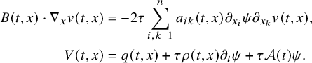 $$ \begin{align*} \begin{aligned} B(t,x)\cdot\nabla_x v(t,x)&=-2\tau\sum_{i,k=1}^na_{ik}(t,x)\partial_{x_i}\psi\partial_{x_k}v(t,x), \\ V(t,x)&=q(t,x)+\tau\rho(t,x)\partial_t \psi+\tau\mathcal A(t)\psi. \end{aligned} \end{align*} $$
Thus, observing that $B\in C^{\infty }([0,T]\times \overline {\Omega })^n$
,
$B\in C^{\infty }([0,T]\times \overline {\Omega })^n$
, $V\in C^{\frac {\alpha }{2},\alpha }([0,T]\times \overline {\Omega })$
,
$V\in C^{\frac {\alpha }{2},\alpha }([0,T]\times \overline {\Omega })$
, $ L_+c_+\in C^\infty _0(0,T;C^\infty (\overline {\Omega }))$
and applying [Reference Ladyženskaja, Solonnikov and Ural’cevaLSU88, Theorem 5.2, Chapter IV, page 320], we deduce that (5.15) admits a unique solution
$ L_+c_+\in C^\infty _0(0,T;C^\infty (\overline {\Omega }))$
and applying [Reference Ladyženskaja, Solonnikov and Ural’cevaLSU88, Theorem 5.2, Chapter IV, page 320], we deduce that (5.15) admits a unique solution $R_{+,\tau }\in C^{1+\frac {\alpha }{2},2+\alpha }([0,T]\times \overline {\Omega })$
, and we only need to check estimate (5.17).
$R_{+,\tau }\in C^{1+\frac {\alpha }{2},2+\alpha }([0,T]\times \overline {\Omega })$
, and we only need to check estimate (5.17).
In this proof, we set
 $$ \begin{align*}v=R_{+,\tau}, \quad K=-L_+c_{+}, \end{align*} $$
and without loss of generality, we assume that both v and K are real valued. We fix $\lambda>0$
, and we multiply (5.15) by
$\lambda>0$
, and we multiply (5.15) by $ve^{\lambda \psi }$
in order to get
$ve^{\lambda \psi }$
in order to get
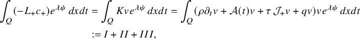 $$ \begin{align*} \int_Q \left(-L_+c_{+} \right) e^{\lambda \psi} \, dxdt &=\int_Q Kve^{\lambda \psi}\, dxdt =\int_Q \left(\rho\partial_tv+\mathcal A(t)v+\tau\, \mathcal J_{+}v+qv\right)ve^{\lambda \psi}\, dxdt\\ &:= I+II+III, \end{align*} $$
where
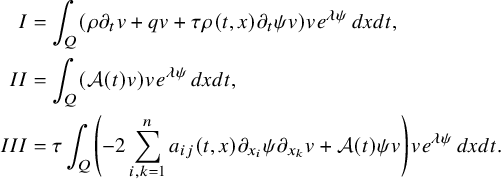 $$ \begin{align*} I&=\int_Q \left(\rho\partial_tv+qv+\tau \rho(t,x)\partial_t \psi v\right)ve^{\lambda \psi}\, dxdt, \\ II&=\int_Q (\mathcal A(t)v)ve^{\lambda \psi}\, dxdt, \\ III&=\tau \int_Q\left(-2 \sum_{i,k=1}^na_{ij}(t,x)\partial_{x_i}\psi\partial_{x_k} v+\mathcal A(t)\psi v\right)ve^{\lambda \psi}\, dxdt. \end{align*} $$
For I, using the fact that $v_{|t=0}=0$
and integrating by parts, we get
$v_{|t=0}=0$
and integrating by parts, we get
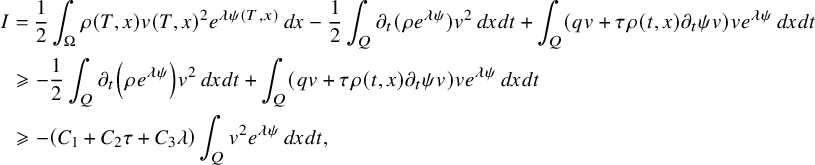 $$ \begin{align*} I&=\frac{1}{2}\int_\Omega \rho(T,x)v(T,x)^2e^{\lambda \psi(T,x)}\, dx-\frac{1}{2}\int_Q\partial_t(\rho e^{\lambda \psi})v^2\, dxdt +\int_Q (qv+\tau \rho(t,x)\partial_t \psi v)ve^{\lambda \psi}\, dxdt\\ &\geqslant -\frac{1}{2}\int_Q\partial_t\left(\rho e^{\lambda \psi}\right)v^2\, dxdt+\int_Q \left(qv+\tau \rho(t,x)\partial_t \psi v\right)ve^{\lambda \psi}\, dxdt\\ &\geqslant -\left(C_1+C_2\tau+C_3\lambda\right) \int_Qv^2e^{\lambda \psi}\, dxdt, \end{align*} $$
with $C_1,C_2, C_3$
three positive constants independent of
$C_1,C_2, C_3$
three positive constants independent of $\lambda $
and
$\lambda $
and $\tau $
.
$\tau $
.
For $II$
, using the fact that
$II$
, using the fact that $v|_{\Sigma }=0$
, applying (1.1) and integrating by parts, we find
$v|_{\Sigma }=0$
, applying (1.1) and integrating by parts, we find
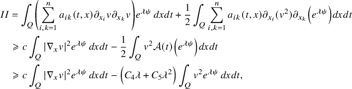 $$ \begin{align*} II&=\int_Q \left(\sum_{i,k=1}^na_{ik}(t,x)\partial_{x_i}v\partial_{x_k} v\right)e^{\lambda \psi}\, dxdt+\frac{1}{2}\int_Q \sum_{i,k=1}^na_{ik}(t,x)\partial_{x_i}(v^2)\partial_{x_k} \left(e^{\lambda \psi}\right)dxdt\\ &\geqslant c\int_Q |\nabla_x v|^2e^{\lambda \psi}\, dxdt-\frac{1}{2}\int_Q v^2\mathcal A(t)\left(e^{\lambda \psi}\right)dxdt\\ &\geqslant c\int_Q |\nabla_x v|^2e^{\lambda \psi}\, dxdt-\left(C_4\lambda+C_5\lambda^2\right) \int_Qv^2e^{\lambda \psi}\, dxdt, \end{align*} $$
with constants $c, C_4,C_5>0$
independent of
$c, C_4,C_5>0$
independent of $\lambda $
and
$\lambda $
and $\tau $
.
$\tau $
.
Finally, for $III$
, using the that
$III$
, using the that $\mathcal I=0$
, with
$\mathcal I=0$
, with $\mathcal I$
defined by (5.7), we find
$\mathcal I$
defined by (5.7), we find
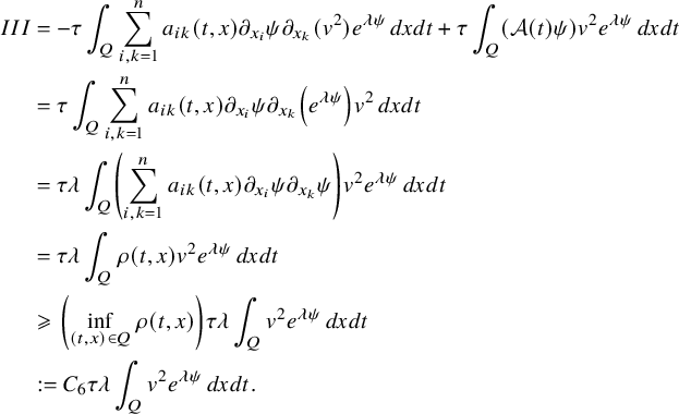 $$ \begin{align*} III&=-\tau \int_Q \sum_{i,k=1}^na_{ik}(t,x)\partial_{x_i}\psi\partial_{x_k} (v^2)e^{\lambda \psi}\, dxdt+\tau \int_Q(\mathcal A(t)\psi) v^2e^{\lambda \psi}\, dxdt\\ &= \tau \int_Q \sum_{i,k=1}^na_{ik}(t,x)\partial_{x_i}\psi\partial_{x_k}\left(e^{\lambda \psi}\right) v^2\, dxdt\\ &= \tau\lambda \int_Q \left(\sum_{i,k=1}^na_{ik}(t,x)\partial_{x_i}\psi\partial_{x_k}\psi\right) v^2e^{\lambda \psi}\, dxdt\\ &= \tau\lambda \int_Q \rho(t,x) v^2e^{\lambda \psi}\, dxdt\\ &\geqslant \left(\inf_{(t,x)\in Q}\rho(t,x)\right)\tau\lambda\int_Q v^2e^{\lambda \psi}\, dxdt\\ &:=C_6\tau\lambda\int_Q v^2e^{\lambda \psi}\, dxdt. \end{align*} $$
Combining these estimates of I, $II$
and
$II$
and $III$
, we find
$III$
, we find
 $$ \begin{align*} \int_Q Kve^{\lambda \psi}\, dxdt &\geqslant c\int_Q |\nabla_x v|^2e^{\lambda \psi}\, dxdt +\left(-C_1-C_2\tau-C_3\lambda-C_4\lambda-C_5\lambda^2+C_6\tau\lambda\right)\int_Q v^2e^{\lambda \psi}\,dxdt. \end{align*} $$
Choosing $\lambda \geqslant \frac {3C_2}{C_6}$
and
$\lambda \geqslant \frac {3C_2}{C_6}$
and
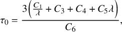 $$ \begin{align*}\tau_0=\frac{3\left(\frac{C_1}{\lambda}+C_3+C_4+C_5\lambda\right)}{C_6},\end{align*} $$
we deduce that
 $$ \begin{align*}\int_Q Kve^{\lambda \psi}\, dxdt\geqslant c\int_Q |\nabla_x v|^2e^{\lambda \psi}\, dxdt+\frac{C_6}{3}\tau\lambda\int_Q v^2e^{\lambda \psi}\, dxdt,\quad \tau>\tau_0.\end{align*} $$
Applying Cauchy-Schwarz inequality, for $\tau>\tau _0$
, we get
$\tau>\tau _0$
, we get
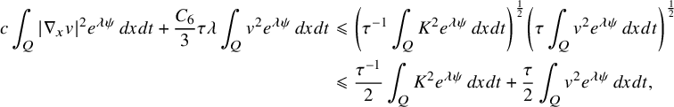 $$ \begin{align*}\begin{aligned} c\int_Q |\nabla_x v|^2e^{\lambda \psi}\, dxdt+\frac{C_6}{3}\tau\lambda\int_Q v^2e^{\lambda \psi}\, dxdt&\leqslant \left(\tau^{-1}\int_Q K^2e^{\lambda \psi}\, dxdt\right)^{\frac{1}{2}}\left(\tau\int_Q v^2e^{\lambda \psi}\, dxdt\right)^{\frac{1}{2}}\\ &\leqslant \frac{\tau^{-1}}{2}\int_Q K^2e^{\lambda \psi}\, dxdt+\frac{\tau}{2}\int_Q v^2e^{\lambda \psi}\, dxdt,\end{aligned}\end{align*} $$
which implies that
 $$ \begin{align*}c\int_Q |\nabla_x v|^2e^{\lambda \psi}\, dxdt+\tau\left(\frac{C_6}{3}\lambda-\frac{1}{2}\right)\int_Q v^2e^{\lambda \psi}\, dxdt\leqslant\frac{\tau^{-1}}{2}\int_Q K^2e^{\lambda \psi}\, dxdt.\end{align*} $$
Fixing $\lambda =\frac {3(C_2+1)}{C_6}$
, we obtain
$\lambda =\frac {3(C_2+1)}{C_6}$
, we obtain
 $$ \begin{align*}\tau\int_Q |\nabla_x v|^2\, dxdt+\tau^2\int_Q v^2\, dxdt\leqslant C\int_Q K^2\, dxdt,\quad \tau>\tau_0,\end{align*} $$
where $C>0$
is a constant independent of
$C>0$
is a constant independent of $\tau $
. From this last estimate, we deduce (5.17).
$\tau $
. From this last estimate, we deduce (5.17).
Note that the the energy estimate (5.17) is only subjected to the requirement that $\psi $
solves the eikonal equation
$\psi $
solves the eikonal equation $\mathcal I=0$
in Q. For this result, the simplicity assumption is not required.
$\mathcal I=0$
in Q. For this result, the simplicity assumption is not required.
Applying Proposition 5.1, we deduce the existence of $R_{\pm ,\tau }$
fulfilling condition (5.15)–(5.16) and the decay estimate (5.14). Armed with these class of GO solutions, we are now in position to complete the proof of Proposition 4.1.
$R_{\pm ,\tau }$
fulfilling condition (5.15)–(5.16) and the decay estimate (5.14). Armed with these class of GO solutions, we are now in position to complete the proof of Proposition 4.1.
5.2 Completion of the proof of Proposition 4.1
We will show Proposition 4.1 by iteration.
Proof of Proposition 4.1.
We start by showing that the claim of Proposition 4.1 holds true for $m=1$
. We fix
$m=1$
. We fix $x_0\in \partial \Omega _1$
,
$x_0\in \partial \Omega _1$
, $t_0\in (0,T)$
and for
$t_0\in (0,T)$
and for $\chi _*\in C^\infty _0(-1,1)$
satisfying
$\chi _*\in C^\infty _0(-1,1)$
satisfying
 $$ \begin{align*}\int_{\mathbb R} \chi_*(t)^2\, dt=1,\end{align*} $$
and we set
 $$ \begin{align*} \chi_\delta (t) =\delta^{-\frac{1}{2}}\chi_*\left(\delta^{-1}(t-t_0)\right), \quad \text{ for }\delta\in \left(0,\min(T-t_0,t_0)\right). \end{align*} $$
We consider $v_1\in C^{1+\frac {\alpha }{2},2+\alpha }([0,T]\times \overline {\Omega })$
(resp.
$v_1\in C^{1+\frac {\alpha }{2},2+\alpha }([0,T]\times \overline {\Omega })$
(resp. $w\in C^{1+\frac {\alpha }{2},2+\alpha }([0,T]\times \overline {\Omega })$
) of the form (5.3) (resp. (5.4)) satisfying (5.1) (resp. (5.2)) with
$w\in C^{1+\frac {\alpha }{2},2+\alpha }([0,T]\times \overline {\Omega })$
) of the form (5.3) (resp. (5.4)) satisfying (5.1) (resp. (5.2)) with $q=q_1$
(resp.
$q=q_1$
(resp. $q=q_0$
) and
$q=q_0$
) and $R_{+,\tau }$
(resp.
$R_{+,\tau }$
(resp. $R_{-,\tau }$
) satisfying the decay property (5.14). Here, we choose
$R_{-,\tau }$
) satisfying the decay property (5.14). Here, we choose $\chi =\chi _\delta $
in the expression of the function
$\chi =\chi _\delta $
in the expression of the function $v_1$
and w. Then, condition (4.1) implies that
$v_1$
and w. Then, condition (4.1) implies that
 $$ \begin{align} \int_0^T\int_\Omega F(t,x)c_{+,0}c_{-,0}\, dx dt=\lim_{\tau\to+\infty}\int_0^T\int_\Omega F(t,x)v_1w \, dx dt=0. \end{align} $$
From now on, for $t\in [0,T]$
, we denote by
$t\in [0,T]$
, we denote by $\partial _+S_t(\overline {\Omega _1})$
the unit sphere bundle
$\partial _+S_t(\overline {\Omega _1})$
the unit sphere bundle
 $$ \begin{align*}\partial _+S_t(\overline{\Omega_1}):=\left\{(x,\theta)\in S_t(\overline{\Omega_1}):\, x\in\partial \Omega_1,\ \left\langle \theta,\nu_t(x)\right\rangle_{g(t)}<0\right\},\end{align*} $$
where $\nu _t$
denotes the outward unit normal vector of
$\nu _t$
denotes the outward unit normal vector of $\partial \Omega _1$
with respect to the metric
$\partial \Omega _1$
with respect to the metric $g(t)$
. We also denote for any
$g(t)$
. We also denote for any $(y,\theta )\in \partial _+S_t(\overline {\Omega _1})$
by
$(y,\theta )\in \partial _+S_t(\overline {\Omega _1})$
by $\ell _{t,+}(y,\theta )$
the time of existence in
$\ell _{t,+}(y,\theta )$
the time of existence in $\overline {\Omega _1}$
of the maximal geodesic
$\overline {\Omega _1}$
of the maximal geodesic $\gamma _{y,\theta }$
, with respect to the metric
$\gamma _{y,\theta }$
, with respect to the metric $g(t)$
, satisfying
$g(t)$
, satisfying $\gamma _{y,\theta }(0)=y$
and
$\gamma _{y,\theta }(0)=y$
and $\gamma _{y,\theta }'(0)=\theta $
.
$\gamma _{y,\theta }'(0)=\theta $
.
Consider $\tilde {F}\in L^\infty ((0,T)\times \Omega _1)$
defined by
$\tilde {F}\in L^\infty ((0,T)\times \Omega _1)$
defined by
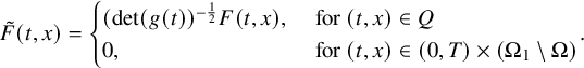 $$ \begin{align*} \tilde{F}(t,x)=\begin{cases} (\det(g(t))^{-\frac{1}{2}}F(t,x), &\text{ for }(t,x)\in Q\\ 0, & \text{ for }(t,x)\in (0,T)\times (\Omega_1\setminus\Omega) \end{cases}. \end{align*} $$
Then we have
 $$ \begin{align*}\int_0^T\int_{\overline{\Omega_1}} \tilde{F}(t,x)c_{+,0}c_{-,0}\, dV_{g(t)}(x) dt=\int_0^T\int_{\Omega_1} \tilde{F}(t,x)c_{+,0}c_{-,0}\sqrt{\det(g(t))}\, dx dt=0,\end{align*} $$
where $dV_{g(t)}$
is the Riemannian volume of
$dV_{g(t)}$
is the Riemannian volume of $(\overline {\Omega _1},g(t))$
. Passing to polar normal coordinates, we obtain
$(\overline {\Omega _1},g(t))$
. Passing to polar normal coordinates, we obtain
 $$ \begin{align*}\int_0^T\chi_\delta(t)^2\int_0^{\ell_{t,+}(y,\theta)}\int_{S_{x_0,t}(\overline{\Omega_1})}h(\theta)\tilde{F}(t,r,\theta)\, d\theta dr dt=0.\end{align*} $$
Using the fact that $F\in C([0,T]\times \overline {\Omega })$
, we deduce that
$F\in C([0,T]\times \overline {\Omega })$
, we deduce that $\tilde {F}\in C([0,T];L^\infty (\Omega _1))$
, and letting
$\tilde {F}\in C([0,T];L^\infty (\Omega _1))$
, and letting $\delta \to 0$
, we obtain
$\delta \to 0$
, we obtain
 $$ \begin{align*}\int_0^{\ell_{t_0,+}(x_0,\theta)}\int_{S_{x_0,t_0}(\overline{\Omega_1})}h(\theta)\tilde{F}(t_0,r,\theta)\, d\theta dr=0.\end{align*} $$
Applying the fact that in this identity $h\in C^\infty ( S_{x_0,t_0}(\overline {\Omega _1}))$
is arbitrary chosen, we deduce that
$h\in C^\infty ( S_{x_0,t_0}(\overline {\Omega _1}))$
is arbitrary chosen, we deduce that
 $$ \begin{align*}\int_0^{\ell_{t_0,+}(x_0,\theta)}\tilde{F}(t_0,\gamma_{x_0,\theta}(s))\, ds=\int_0^{\ell_{t_0,+}(x_0,\theta)}\tilde{F}(t_0,r,\theta)\, dr=0,\quad (x_0,\theta)\in \partial _+S_{t_0}(\overline{\Omega_1}).\end{align*} $$
Combining this with the facts that in this identity, $x_0\in \partial \Omega _1$
was arbitrary chosen, that the manifold
$x_0\in \partial \Omega _1$
was arbitrary chosen, that the manifold $ (\overline {\Omega _1},g(t_0) )$
is assumed to be simple and that the geodesic ray transform is injective on simple manifolds, we deduce that
$ (\overline {\Omega _1},g(t_0) )$
is assumed to be simple and that the geodesic ray transform is injective on simple manifolds, we deduce that $\tilde {F}(t_0,\,\cdot \,)\equiv 0$
on
$\tilde {F}(t_0,\,\cdot \,)\equiv 0$
on $\Omega _1$
. Thus,
$\Omega _1$
. Thus, $F(t_0,\,\cdot \,)\equiv 0$
. Combining this with the fact that here
$F(t_0,\,\cdot \,)\equiv 0$
. Combining this with the fact that here $t_0\in (0,T)$
is arbitrary chosen and
$t_0\in (0,T)$
is arbitrary chosen and $F\in C([0,T]\times \overline {\Omega })$
, we deduce that
$F\in C([0,T]\times \overline {\Omega })$
, we deduce that $F\equiv 0$
.
$F\equiv 0$
.
Now let us fix $m\geqslant 1$
, and assume that (4.1) for this m implies that
$m\geqslant 1$
, and assume that (4.1) for this m implies that $F\equiv 0$
. Fix
$F\equiv 0$
. Fix $G\in C([0,T]\times \overline {\Omega })$
, and assume that
$G\in C([0,T]\times \overline {\Omega })$
, and assume that
 $$ \begin{align*}\int_0^T\int_\Omega Gv_1\cdots v_{m+1}\hspace{0.5pt} w\, dxdt=0\end{align*} $$
for all $v_1,\ldots , v_{m+1}\in C^{1+\frac {\alpha }{2},2+\alpha }([0,T]\times \overline {\Omega }))$
satisfying (4.2) and all
$v_1,\ldots , v_{m+1}\in C^{1+\frac {\alpha }{2},2+\alpha }([0,T]\times \overline {\Omega }))$
satisfying (4.2) and all $w\in C^{1+\frac {\alpha }{2},2+\alpha }([0,T]\times \overline {\Omega }))$
satisfying (4.3). Fixing
$w\in C^{1+\frac {\alpha }{2},2+\alpha }([0,T]\times \overline {\Omega }))$
satisfying (4.3). Fixing $F=Gv_1$
, we deduce that
$F=Gv_1$
, we deduce that $F\equiv 0$
, and multiplying F by an arbitrary chosen
$F\equiv 0$
, and multiplying F by an arbitrary chosen $w\in C^{1+\frac {\alpha }{2},2+\alpha }([0,T]\times \overline {\Omega }))$
satisfying (4.3), and integrating, we deduce that
$w\in C^{1+\frac {\alpha }{2},2+\alpha }([0,T]\times \overline {\Omega }))$
satisfying (4.3), and integrating, we deduce that
 $$ \begin{align*}\int_0^T\int_\Omega Gv_1 w\, dxdt=0\end{align*} $$
for all $v_1\in C^{1+\frac {\alpha }{2},2+\alpha }([0,T]\times \overline {\Omega }))$
satisfying (4.2) and all
$v_1\in C^{1+\frac {\alpha }{2},2+\alpha }([0,T]\times \overline {\Omega }))$
satisfying (4.2) and all $w\in C^{1+\frac {\alpha }{2},2+\alpha }([0,T]\times \overline {\Omega }))$
satisfying (4.3). Then, the above argumentation implies that
$w\in C^{1+\frac {\alpha }{2},2+\alpha }([0,T]\times \overline {\Omega }))$
satisfying (4.3). Then, the above argumentation implies that $G\equiv 0$
. This proves the assertion.
$G\equiv 0$
. This proves the assertion.
6 Proof of Theorem 2.2
In this section, we assume that $n\geqslant 3$
and
$n\geqslant 3$
and $\psi (x)=|x-x_0|$
,
$\psi (x)=|x-x_0|$
, $x\in \Omega $
, for
$x\in \Omega $
, for $x_0\in {\mathbb R}^n\setminus \overline {\Omega }$
. Note that the function
$x_0\in {\mathbb R}^n\setminus \overline {\Omega }$
. Note that the function $\psi $
satisfies the eikonal equation
$\psi $
satisfies the eikonal equation
 $$ \begin{align} \left|\nabla_x \psi(x)\right|=1, \text{ for }x\in \Omega. \end{align} $$
We start by considering the following new Carleman estimate whose proof is postponed to Appendix A.
Lemma 6.1. Let $q\in L^\infty (Q)$
and
$q\in L^\infty (Q)$
and $v\in H^1(Q)\cap L^2(0,T;H^2(\Omega ))$
satisfy the condition
$v\in H^1(Q)\cap L^2(0,T;H^2(\Omega ))$
satisfy the condition
 $$ \begin{align}v|_{\Sigma}=0,\quad v|_{t=0}=0.\end{align} $$
Then, there exists $\tau _0>0$
depending on T,
$\tau _0>0$
depending on T, $\Omega $
and
$\Omega $
and $\left \lVert q\right \rVert _{L^\infty (Q)}$
such that for all
$\left \lVert q\right \rVert _{L^\infty (Q)}$
such that for all $\tau>\tau _0$
, the following estimate
$\tau>\tau _0$
, the following estimate
 $$ \begin{align} \begin{aligned} &\tau\int_0^T\int_{\Gamma_{+}(x_0)}e^{-2(\tau^2t+\tau\psi(x))}\left\lvert\partial_\nu v\right\rvert^2\left\lvert\partial_\nu\psi(x) \right\rvert d\sigma(x)dt+\tau^2\int_Qe^{-2(\tau^2t+\tau\psi(x))}\left\lvert v\right\rvert^2dxdt\\ &\quad \leqslant C\left(\int_Qe^{-2(\tau^2t+\tau\psi(x))}\left\lvert(\partial_t-\Delta_x+q)v\right\rvert^2\, dxdt \right. \\ &\qquad \left. +\,\tau\int_0^T\int_{\Gamma_{-}(x_0)}e^{-2(\tau^2t+\tau\psi(x))}\left\lvert\partial_\nu v\right\rvert^2\left\lvert\partial_\nu\psi(x) \right\rvert d\sigma(x)\, dt\right) \end{aligned}\end{align} $$
holds true.
Remark 6.1. The weight function $\psi $
under consideration in the Carleman estimates (6.3) is chosen in accordance with the construction of geometric optics solutions of the form (5.3)–(5.4) introduced in Section 5.1. Namely, we need to consider weight functions
$\psi $
under consideration in the Carleman estimates (6.3) is chosen in accordance with the construction of geometric optics solutions of the form (5.3)–(5.4) introduced in Section 5.1. Namely, we need to consider weight functions $\psi $
that can be the phase of such geometric optics solutions. For this reason, we need to consider weight functions that satisfy the eikonal equation
$\psi $
that can be the phase of such geometric optics solutions. For this reason, we need to consider weight functions that satisfy the eikonal equation $\mathcal I=0$
which takes the form (6.1) in the context of Theorem 2.2.
$\mathcal I=0$
which takes the form (6.1) in the context of Theorem 2.2.
Armed with these results, we are now in a position to complete the proof of Theorem 2.2.
Proof of Theorem 2.2.
Following the proof of Theorem 2.1, we only need to prove that (4.4) holds true. We will prove this by a recursion argument. Let us first observe that since $\tilde {\Gamma }$
is a neighborhood of
$\tilde {\Gamma }$
is a neighborhood of $\Gamma _-(x_0)$
, there exists
$\Gamma _-(x_0)$
, there exists $\epsilon>0$
such that
$\epsilon>0$
such that $B(x_0,\epsilon )\cap \overline {\Omega }=\emptyset $
, and for all
$B(x_0,\epsilon )\cap \overline {\Omega }=\emptyset $
, and for all $y\in B(x_0,\epsilon )$
, we have
$y\in B(x_0,\epsilon )$
, we have
 $$ \begin{align*}\Gamma_-(y,\epsilon):=\left\{x\in\partial\Omega:\ (x-y)\cdot\nu(x)\leqslant\epsilon\right\}\subset \tilde{\Gamma}. \end{align*} $$
We start by considering (4.4) for $k=1$
. For
$k=1$
. For $j=1,2$
, consider
$j=1,2$
, consider $v_{j,1}\in C^{1+\frac {\alpha }{2},2+\alpha }([0,T]\times \overline {\Omega }))$
satisfying (4.2) with
$v_{j,1}\in C^{1+\frac {\alpha }{2},2+\alpha }([0,T]\times \overline {\Omega }))$
satisfying (4.2) with $b=b_j$
and
$b=b_j$
and $w\in C^{1+\frac {\alpha }{2},2+\alpha }([0,T]\times \overline {\Omega }))$
satisfying (4.3) with
$w\in C^{1+\frac {\alpha }{2},2+\alpha }([0,T]\times \overline {\Omega }))$
satisfying (4.3) with $b=b_1$
. We assume here that
$b=b_1$
. We assume here that $v_{1,1}|_{\Sigma }=h=v_{2,1}|_{\Sigma }$
for some
$v_{1,1}|_{\Sigma }=h=v_{2,1}|_{\Sigma }$
for some $h\in \mathcal K_0$
. Fixing
$h\in \mathcal K_0$
. Fixing $v_1=v_{1,1}-v_{2,1}$
, we deduce that
$v_1=v_{1,1}-v_{2,1}$
, we deduce that $v_1$
satisfies the conditions
$v_1$
satisfies the conditions
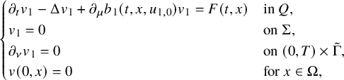 $$ \begin{align*} \begin{cases} \partial_t v_1-\Delta v_1+ \partial_\mu b_1(t,x,u_{1,0})v_1 =F(t,x) & \mbox{in}\ Q , \\ v_1=0 &\mbox{on}\ \Sigma,\\ \partial_{\nu}v_1=0 &\mbox{on}\ (0,T)\times \tilde \Gamma,\\ v(0,x)=0 &\mbox{for } x\in\Omega, \end{cases} \end{align*} $$
with
 $$ \begin{align*}F(t,x)=\left(\partial_\mu b_2(t,x,u_{2,0}(t,x))-\partial_\mu b_1(t,x,u_{1,0}(t,x))\right)v_{2,1}(t,x),\quad (t,x)\in Q.\end{align*} $$
Multiplying the above equation by w and integrating by parts, we obtain
 $$ \begin{align*}\int_0^T\int_{\Omega}\left(\partial_\mu b_2(t,x,u_{2,0})-\partial_\mu b_1(t,x,u_{1,0})\right)v_{2,1}w \, dx dt-\int_{\Sigma}\partial_\nu v_1(t,x) w(t,x)\, d\sigma(x)dt=0.\end{align*} $$
Moreover, applying the first-order linearization, we find
 $$ \begin{align*} \quad \, \left.\partial_{\nu} v_{1,1}\right|{}_{(0,T)\times \Gamma_-(y,\epsilon)}&=\left.\partial_s\mathcal N_{b_1}(f_0+sh)\right|{}_{(0,T)\times \Gamma_-(y,\epsilon)}\\ &=\left.\partial_s\mathcal N_{b_2}(f_0+sh)\right|{}_{(0,T)\times \Gamma_-(y,\epsilon)}\\ &=\left.\partial_{\nu} v_{2,1}\right|{}_{(0,T)\times \Gamma_-(y,\epsilon)}, \end{align*} $$
and it follows that
 $$ \begin{align} \begin{aligned} &\int_0^T\int_{\Omega}(\partial_\mu b_2(t,x,u_{2,0})-\partial_\mu b_1(t,x,u_{1,0}))v_{2,1}w \, dx dt\\ =&\int_0^T\int_{\partial\Omega\setminus \Gamma_-(y,\epsilon)}\partial_\nu v_1(t,x) w(t,x) \, d\sigma(x) dt, \end{aligned} \end{align} $$
with $v_{2,1}$
(resp. w) an arbitrary chosen element of
$v_{2,1}$
(resp. w) an arbitrary chosen element of $C^{1+\frac {\alpha }{2},2+\alpha }([0,T]\times \overline {\Omega }))$
satisfying (4.2) (resp. (4.3)). In particular, we can apply this identity to
$C^{1+\frac {\alpha }{2},2+\alpha }([0,T]\times \overline {\Omega }))$
satisfying (4.2) (resp. (4.3)). In particular, we can apply this identity to $v_{2,1}$
and w two GO solutions of the form (5.3) and (5.4) with
$v_{2,1}$
and w two GO solutions of the form (5.3) and (5.4) with $\psi (x)=|x-y|$
and
$\psi (x)=|x-y|$
and $c_\pm $
given by
$c_\pm $
given by
 $$ \begin{align*} c_{+}(t,x)&=\chi_\delta(t)h\left(\frac{x-y}{|x-y|}\right)|x-y|^{-(n-1)/2},\\ c_{-}(t,x)&=\chi_\delta(t)|x-y|^{-(n-1)/2}, \end{align*} $$
for $(t,x)\in [0,T]\times ({\mathbb R}^n\setminus \{y\})$
with
$(t,x)\in [0,T]\times ({\mathbb R}^n\setminus \{y\})$
with $h\in C^\infty (\mathbb S^{n-1})$
and
$h\in C^\infty (\mathbb S^{n-1})$
and
 $$ \begin{align*}\chi_\delta (t) =\delta^{-\frac{1}{2}}\chi_*(\delta^{-1}(t-t_0)), \text{ for }\delta\in(0,\min(T-t_0,t_0)),\end{align*} $$
where $\chi _*\in C^\infty _0(-1,1)$
satisfies
$\chi _*\in C^\infty _0(-1,1)$
satisfies
 $$ \begin{align*}\int_{\mathbb R} \chi_*(t)^2\, dt=1.\end{align*} $$
Note that the construction of such GO solutions is a consequence of the fact that we can find $\Omega _2$
an open neighborhood of
$\Omega _2$
an open neighborhood of $\overline {\Omega }$
such that
$\overline {\Omega }$
such that $\psi \in C^\infty (\overline {\Omega _2})$
solves the eikonal equation
$\psi \in C^\infty (\overline {\Omega _2})$
solves the eikonal equation
 $$ \begin{align*}\left|\nabla_x\psi(x)\right|{}^2=1,\quad x\in\Omega_2,\end{align*} $$
as well as an application of Proposition 5.1. In addition, we built this class of GO solutions by following the arguments used in Section 5.1 where the polar normal coordinates will be replaced by polar coordinates centered at y. Note that in such coordinates, $\psi =r$
and the transport equations (5.11) are just
$\psi =r$
and the transport equations (5.11) are just
 $$ \begin{align*}\partial_r c_\pm + \left(\frac{\partial_r\beta}{4\beta}\right) c_\pm=0, \end{align*} $$
where $\beta $
is an angle dependent multiple of
$\beta $
is an angle dependent multiple of $r^{2(n-1)}$
.
$r^{2(n-1)}$
.
With this choice of the functions $v_{2,1}$
and w, we obtain by Cauchy-Schwarz inequality that
$v_{2,1}$
and w, we obtain by Cauchy-Schwarz inequality that
 $$ \begin{align} \begin{aligned} &\quad\, \left\lvert\int_0^T\int_{\partial\Omega\setminus \Gamma_-(y,\epsilon)}\partial_\nu v_1(t,x) w(t,x)\, d\sigma(x)dt\right\rvert \\ &\leqslant C\left(\int_0^T\int_{\partial\Omega\setminus \Gamma_-(y,\epsilon)}|\partial_\nu v_1(t,x)|^2e^{-2(\tau^2t+\tau\psi(x))} d\sigma(x)dt\right)^{\frac{1}{2}}. \end{aligned} \end{align} $$
In addition, the Carleman estimate (6.3) and the fact that $\left. \partial _\nu v_1\right |{}_{(0,T)\times \Gamma _-(y)}=0$
imply that, for
$\left. \partial _\nu v_1\right |{}_{(0,T)\times \Gamma _-(y)}=0$
imply that, for $\tau>0$
sufficiently large, we have
$\tau>0$
sufficiently large, we have
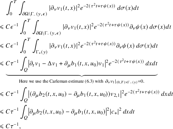 $$ \begin{align*}\begin{aligned} & \quad \, \int_0^T\int_{\partial\Omega\setminus \Gamma_-(y,\epsilon)}|\partial_\nu v_1(t,x)|^2e^{-2(\tau^2t+\tau\psi(x))} \, d\sigma(x)dt\\ &\leqslant C\epsilon^{-1}\int_0^T\int_{\partial\Omega\setminus \Gamma_-(y,\epsilon)}|\partial_\nu v_1(t,x)|^2e^{-2(\tau^2t+\tau\psi(x))}\partial_\nu\psi(x) \, d\sigma(x)dt\\ &\leqslant C\epsilon^{-1}\int_0^T\int_{ \Gamma_+(y)}|\partial_\nu v_1(t,x)|^2e^{-2(\tau^2t+\tau\psi(x))}\partial_\nu\psi(x) \, d\sigma(x)dt\\ &\leqslant \underbrace{C\tau^{-1}\int_Q \left|\partial_t v_1-\Delta v_1+ \partial_\mu b_1(t,x,u_0)v_1\right|{}^2e^{-2(\tau^2t+\tau\psi(x))}\, dxdt}_{\text{Here we use the Carleman estimate (6.3) with }\left.\partial_\nu v_1\right|{}_{(0,T)\times\Gamma_-(y)}=0.}\\ &\leqslant C\tau^{-1}\int_Q \left|(\partial_\mu b_2(t,x,u_0)-\partial_\mu b_1(t,x,u_0))v_{2,1}\right|{}^2e^{-2(\tau^2t+\tau\psi(x))}\, dxdt\\ &\leqslant C\tau^{-1}\int_Q\left|\partial_\mu b_2(t,x,u_0)-\partial_\mu b_1(t,x,u_0)\right|{}^2|c_+|^2\, dxdt\\ &\leqslant C\tau^{-1},\end{aligned}\end{align*} $$
where $C>0$
is a constant independent of
$C>0$
is a constant independent of $\tau $
. Therefore, for
$\tau $
. Therefore, for $\tau>0$
sufficiently large, we obtain
$\tau>0$
sufficiently large, we obtain
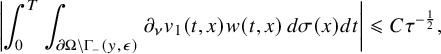 $$ \begin{align*}\left\lvert\int_0^T\int_{\partial\Omega\setminus \Gamma_-(y,\epsilon)}\partial_\nu v_1(t,x) w(t,x)\, d\sigma(x) dt\right\rvert\leqslant C\tau^{-\frac{1}{2}},\end{align*} $$
and in a similar way to Proposition 4.1, sending $\tau \to +\infty $
, we find
$\tau \to +\infty $
, we find
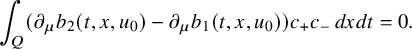 $$ \begin{align*}\int_Q(\partial_\mu b_2(t,x,u_0)-\partial_\mu b_1(t,x,u_0))c_+c_-\, dxdt=0.\end{align*} $$
By using the polar coordinates, sending $\delta \to 0$
and repeating the arguments of Proposition 4.1, one can get
$\delta \to 0$
and repeating the arguments of Proposition 4.1, one can get
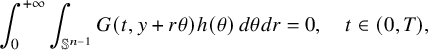 $$ \begin{align*}\int_0^{+\infty}\int_{\mathbb S^{n-1}} G(t,y+r\theta)h(\theta)\, d\theta dr=0,\quad t\in(0,T),\end{align*} $$
where $G:=\partial _\mu b_2(t,x,u_{2,0})-\partial _\mu b_1(t,x,u_{1,0})$
in Q extended to
$G:=\partial _\mu b_2(t,x,u_{2,0})-\partial _\mu b_1(t,x,u_{1,0})$
in Q extended to $(0,T)\times {\mathbb R}^n$
by zero.
$(0,T)\times {\mathbb R}^n$
by zero.
Using the fact that $h\in C^\infty (\mathbb S^{n-1})$
is arbitrary chosen, we get
$h\in C^\infty (\mathbb S^{n-1})$
is arbitrary chosen, we get
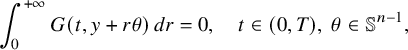 $$ \begin{align*}\int_0^{+\infty} G(t,y+r\theta)\, dr=0,\quad t\in(0,T),\ \theta\in\mathbb S^{n-1}, \end{align*} $$
and the condition on the support of G implies that
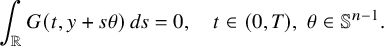 $$ \begin{align*}\int_{\mathbb R} G(t,y+s\theta) \, ds=0,\quad t\in(0,T),\ \theta\in\mathbb S^{n-1}.\end{align*} $$
Since this last identity holds true for all $y\in B(x_0,\epsilon )$
, we obtain
$y\in B(x_0,\epsilon )$
, we obtain
 $$ \begin{align}\int_{\mathbb R} G(t,y+s\theta)\, ds=0,\quad t\in(0,T),\ \theta\in\mathbb S^{n-1},\ y\in B(x_0,\epsilon).\end{align} $$
In addition, since $G=0$
on
$G=0$
on $(0,T)\times {\mathbb R}^n\setminus Q$
, we know that
$(0,T)\times {\mathbb R}^n\setminus Q$
, we know that
 $$ \begin{align*}G(t,x)=0,\quad t\in(0,T),\ x\in B(x_0,\epsilon)\end{align*} $$
and, combining this with (6.6), we are in position to apply [Reference Ilmavirta and MönkkönenIM20, Theorem 1.2] in order to deduce that, for all $t\in (0,T)$
,
$t\in (0,T)$
, $G(t,\cdot )\equiv 0$
. It follows that
$G(t,\cdot )\equiv 0$
. It follows that $G\equiv 0$
and (4.4) holds true for
$G\equiv 0$
and (4.4) holds true for $k=1$
.
$k=1$
.
Now, let us fix $m\in \mathbb N$
and assume that (4.4) holds true for
$m\in \mathbb N$
and assume that (4.4) holds true for $k=1,\ldots ,m$
. Consider
$k=1,\ldots ,m$
. Consider $v_1,\ldots ,v_{m+1}\in C^{1+\frac {\alpha }{2},2+\alpha }([0,T]\times \overline {\Omega }))$
satisfying (4.2) with
$v_1,\ldots ,v_{m+1}\in C^{1+\frac {\alpha }{2},2+\alpha }([0,T]\times \overline {\Omega }))$
satisfying (4.2) with $b=b_1$
and
$b=b_1$
and $w\in C^{1+\frac {\alpha }{2},2+\alpha }([0,T]\times \overline {\Omega }))$
satisfying (4.2) with
$w\in C^{1+\frac {\alpha }{2},2+\alpha }([0,T]\times \overline {\Omega }))$
satisfying (4.2) with $b=b_1$
. We fix
$b=b_1$
. We fix $h_j=v_j|_{\Sigma }$
,
$h_j=v_j|_{\Sigma }$
, $j=1,\ldots ,m+1$
, and proceeding to the higher-order linearization described in Lemma 3.1, we obtain
$j=1,\ldots ,m+1$
, and proceeding to the higher-order linearization described in Lemma 3.1, we obtain
 $$ \begin{align*}\left.\partial_{\nu(a)} w^{(m+1)}_j\right|{}_{\Sigma}=\left.\partial_{s_{1}}\ldots\partial_{s_{m+1}}\mathcal N_{b_j}(f_0+s_1h_1+\ldots+s_{m+1}h_{m+1})\right|{}_{s=0},\end{align*} $$
with $s=(s_1,\ldots ,s_{m+1})$
and
$s=(s_1,\ldots ,s_{m+1})$
and $w^{(m+1)}_j$
solving (3.9) with
$w^{(m+1)}_j$
solving (3.9) with $b=b_j$
for
$b=b_j$
for $j=1,2$
. Then, (2.6) implies
$j=1,2$
. Then, (2.6) implies
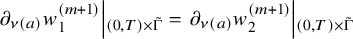 $$ \begin{align*}\left.\partial_{\nu(a)} w^{(m+1)}_1\right|{}_{(0,T)\times \tilde{\Gamma}}=\left.\partial_{\nu(a)} w^{(m+1)}_2\right|{}_{(0,T)\times \tilde{\Gamma}}\end{align*} $$
and, fixing $w^{(m+1)}=w^{(m+1)}_1-w^{(m+1)}_2$
in Q, and applying Lemma 3.1, we deduce that
$w^{(m+1)}=w^{(m+1)}_1-w^{(m+1)}_2$
in Q, and applying Lemma 3.1, we deduce that $w^{(m+1)}$
satisfies the condition
$w^{(m+1)}$
satisfies the condition
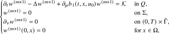 $$ \begin{align*} \begin{cases} \partial_t w^{(m+1)}-\Delta w^{(m+1)}+ \partial_\mu b_1(t,x,u_0) w^{(m+1)}=\mathcal K & \mbox{ in } Q, \\ w^{(m+1)}=0 &\mbox{ on }\Sigma, \\ \partial_{\nu} w^{(m+1)}=0 &\mbox{ on }(0,T)\times \tilde{\Gamma}, \\ w^{(m+1)}(0,x)=0 &\mbox{ for } x\in\Omega, \end{cases} \end{align*} $$
where $\mathcal K= (\partial _\mu ^{m+1} b_2(t,x,u_{2,0})-\partial _\mu ^{m+1} b_1(t,x,u_{1,0}) )v_{1}\cdot \ldots \cdot v_{m+1}$
. Multiplying this equation by w and integrating by parts, we obtain
$\mathcal K= (\partial _\mu ^{m+1} b_2(t,x,u_{2,0})-\partial _\mu ^{m+1} b_1(t,x,u_{1,0}) )v_{1}\cdot \ldots \cdot v_{m+1}$
. Multiplying this equation by w and integrating by parts, we obtain
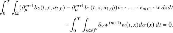 $$ \begin{align*}\begin{aligned}\int_0^T\int_\Omega (\partial_\mu^{m+1} b_2(t,x,u_{2,0})-\partial_\mu^{m+1} b_1(t,x,u_{1,0}))v_1\cdot\ldots\cdot v_{m+1}\cdot w\, dxdt\\ \quad -\int_0^T\int_{\partial\Omega\setminus \tilde{\Gamma}}\partial_\nu w^{(m+1)} w(t,x)d\sigma(x)\, dt=0.\end{aligned}\end{align*} $$
We choose $v_{m+1}$
and w two GO solutions of the form (5.3) and (5.4) with
$v_{m+1}$
and w two GO solutions of the form (5.3) and (5.4) with $\psi (x)=|x-y|$
,
$\psi (x)=|x-y|$
, $y\in B(x_0,\epsilon )$
, and we fix
$y\in B(x_0,\epsilon )$
, and we fix
 $$ \begin{align*}H(t,x)=\left(\partial_\mu^{m+1} b_2(t,x,u_{2,0})-\partial_\mu^{m+1} b_1(t,x,u_{1,0})\right)v_{1}\cdot\ldots\cdot v_{m}(t,x),\quad (t,x)\in Q\end{align*} $$
that we extend by zero to $(0,T)\times {\mathbb R}^n$
. Applying Cauchy-Schwarz inequality and the fact that
$(0,T)\times {\mathbb R}^n$
. Applying Cauchy-Schwarz inequality and the fact that $\Gamma _-(y,\epsilon )\subset \tilde {\Gamma }$
, we find
$\Gamma _-(y,\epsilon )\subset \tilde {\Gamma }$
, we find
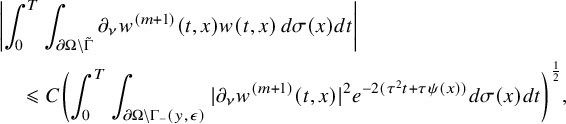 $$ \begin{align*} \begin{aligned} &\left\lvert\int_0^T\int_{\partial\Omega\setminus \tilde{\Gamma}}\partial_\nu w^{(m+1)}(t,x) w(t,x)\, d\sigma(x)dt\right\rvert \\ &\quad \leqslant C\left(\int_0^T\int_{\partial\Omega\setminus \Gamma_-(y,\epsilon)}|\partial_\nu w^{(m+1)}(t,x)|^2e^{-2(\tau^2t+\tau\psi(x))} d\sigma(x)dt\right)^{\frac{1}{2}}, \end{aligned} \end{align*} $$
and, applying the Carleman estimate (6.3) and repeating the above argumentation, we have
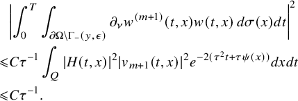 $$ \begin{align*} \begin{split} &\left\lvert\int_0^T\int_{\partial\Omega\setminus \Gamma_-(y,\epsilon)}\partial_\nu w^{(m+1)}(t,x) w(t,x)\, d\sigma(x)dt\right\rvert^2 \\ \leqslant & C\tau^{-1}\int_Q|H(t,x)|^2|v_{m+1}(t,x)|^2e^{-2(\tau^2t+\tau\psi(x))} dxdt\\ \leqslant & C\tau^{-1}. \end{split} \end{align*} $$
Thus, we obtain
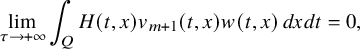 $$ \begin{align*}\lim_{\tau\to+\infty}\int_Q H(t,x) v_{m+1}(t,x) w(t,x)\, dxdt=0,\end{align*} $$
and repeating the above argumentation, we get
 $$ \begin{align*}\left(\partial_\mu^{m+1} b_2(t,x,u_{2,0})-\partial_\mu^{m+1} b_1(t,x,u_{1,0})\right)v_{1}\cdot\ldots\cdot v_{m}(t,x)=H(t,x)=0,\quad (t,x)\in Q.\end{align*} $$
Multiplying this expression by any $w\in C^{1+\frac {\alpha }{2},2+\alpha }([0,T]\times \overline {\Omega }))$
satisfying (4.2) with
$w\in C^{1+\frac {\alpha }{2},2+\alpha }([0,T]\times \overline {\Omega }))$
satisfying (4.2) with $b=b_1$
, we obtain
$b=b_1$
, we obtain
 $$ \begin{align*}\int_Q \left(\partial_\mu^{m+1} b_2(t,x,u_{2,0})-\partial_\mu^{m+1} b_1(t,x,u_{1,0})\right)v_{1}\cdot\ldots\cdot v_{m}w\, dxdt=0,\end{align*} $$
and applying Proposition 4.1, we can conclude that (4.4) holds true for $k=1,\ldots ,m+1$
. It follows that (4.4) holds true for all
$k=1,\ldots ,m+1$
. It follows that (4.4) holds true for all $k\in \mathbb N$
, and repeating the arguments used in the second step of the proof of Theorem 2.1, we can conclude that (2.6) implies (2.5) with the function
$k\in \mathbb N$
, and repeating the arguments used in the second step of the proof of Theorem 2.1, we can conclude that (2.6) implies (2.5) with the function $\varphi =u_{2,0}-u_{1,0}$
satisfying (2.7)–(2.8).
$\varphi =u_{2,0}-u_{1,0}$
satisfying (2.7)–(2.8).
7 Breaking the gauge class
This section is devoted to the proof of the positive answers that we give to problem (IP2) in the theorems and corollaries of Section 2.2.
Proof of Corollary 2.1.
We start by assuming that the conditions of Theorem 2.1 are fulfilled and by proving that (2.4) implies $b_1=b_2$
. By Theorem 2.1, condition (2.4) implies that there exists
$b_1=b_2$
. By Theorem 2.1, condition (2.4) implies that there exists $\varphi \in C^{1+\frac {\alpha }{2},2+\alpha }([0,T]\times \overline {\Omega })$
satisfying (1.6) such that
$\varphi \in C^{1+\frac {\alpha }{2},2+\alpha }([0,T]\times \overline {\Omega })$
satisfying (1.6) such that
 $$ \begin{align} b_1(t,x,\mu)=b_2(t,x,\mu+\varphi(t,x))+\rho(t,x) \partial_t \varphi(t,x)+\mathcal A(t) \varphi(t,x),\quad (t,x,\mu)\in Q\times{\mathbb R}. \end{align} $$
We will prove that $\varphi \equiv 0$
, which implies that
$\varphi \equiv 0$
, which implies that $b_1=b_2$
. Choosing
$b_1=b_2$
. Choosing $\mu =\kappa (t,x)$
and applying (2.10), we obtain
$\mu =\kappa (t,x)$
and applying (2.10), we obtain
 $$ \begin{align*}\begin{aligned} \quad\, \rho(t,x) \partial_t \varphi(t,x)+\mathcal A(t) \varphi(t,x)+b_2(t,x,\kappa(t,x)+\varphi(t,x))-b_2(t,x,\kappa(t,x))\\ =b_1(t,x,\kappa(t,x))-b_2(t,x,\kappa(t,x))=0,\quad (t,x)\in Q.\end{aligned}\end{align*} $$
Moreover, we have
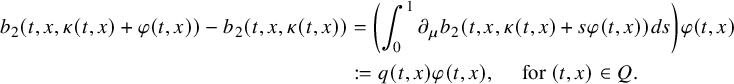 $$ \begin{align*}\begin{aligned} b_2(t,x,\kappa(t,x)+\varphi(t,x))-b_2(t,x,\kappa(t,x))& =\left(\int_0^1\partial_\mu b_2(t,x,\kappa(t,x)+s\varphi(t,x))ds\right)\varphi(t,x)\\ &:=q(t,x)\varphi(t,x),\quad \text{ for } (t,x)\in Q.\end{aligned}\end{align*} $$
Therefore, $\varphi $
fulfills the condition
$\varphi $
fulfills the condition
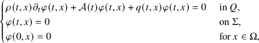 $$ \begin{align} \begin{cases} \rho(t,x) \partial_t \varphi(t,x)+\mathcal A(t) \varphi(t,x)+q(t,x)\varphi(t,x) = 0 & \text{ in } Q,\\ \varphi(t,x) = 0 & \text{ on } \Sigma,\\ \varphi(0,x) = 0 & \text{ for } x \in \Omega, \end{cases} \end{align} $$
and the uniqueness of solutions for this problem implies that $\varphi \equiv 0$
. Thus, (7.1) implies
$\varphi \equiv 0$
. Thus, (7.1) implies $b_1=b_2$
.
$b_1=b_2$
.
Using similar arguments, one can check that, by assuming the conditions of Theorem 2.2, (2.6) implies also that $b_1=b_2$
.
$b_1=b_2$
.
Proof of Corollary 2.2.
Let us assume that the conditions of Theorem 2.1 and (2.4) are fulfilled. By Theorem 2.1 there exists $\varphi \in C^{1+\frac {\alpha }{2},2+\alpha }([0,T]\times \overline {\Omega })$
satisfying (1.6) such that (7.1) is fulfilled. In particular, by choosing
$\varphi \in C^{1+\frac {\alpha }{2},2+\alpha }([0,T]\times \overline {\Omega })$
satisfying (1.6) such that (7.1) is fulfilled. In particular, by choosing $\mu =0$
, we have
$\mu =0$
, we have
 $$ \begin{align*}b_1(t,x,0)-b_2(t,x,0)=b_2(t,x,\varphi(t,x))-b_2(t,x,0)+\rho(t,x) \partial_t \varphi(t,x)+\mathcal A(t) \varphi(t,x)\text{ in } Q.\end{align*} $$
Combining this with (2.12) and (1.6), we deduce that $\varphi $
fulfills the condition
$\varphi $
fulfills the condition
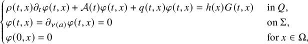 $$ \begin{align} \begin{cases} \rho(t,x) \partial_t \varphi(t,x)+\mathcal A(t) \varphi(t,x)+q(t,x)\varphi(t,x) = h(x)G(t,x) & \text{ in } Q,\\ \varphi(t,x)=\partial_{\nu(a)}\varphi(t,x) = 0 & \text{ on }\Sigma,\\ \varphi(0,x) = 0 & \text{ for }x \in \Omega, \end{cases} \end{align} $$
with
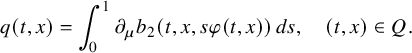 $$ \begin{align*}q(t,x)=\int_0^1\partial_\mu b_2(t,x,s\varphi(t,x))\, ds,\quad (t,x)\in Q.\end{align*} $$
Moreover, following the proof of Theorem 2.1, we know that $\varphi =u_{2,0}-u_{1,0}$
and the additional assumption (2.13)
$\varphi =u_{2,0}-u_{1,0}$
and the additional assumption (2.13)
 $$\begin{align*}u_{1,0}(\theta,x)=u_{2,0}(\theta,x) \end{align*}$$
implies that
 $$ \begin{align*}\varphi(\theta,x)=0,\quad x\in\Omega.\end{align*} $$
Combining this with (2.11),
 $$\begin{align*}\inf_{x\in \Omega}\left\lvert G(\theta,x)\right\rvert>0, \end{align*}$$
(7.3) and applying [Reference Imanuvilov and YamamotoIY98, Theorem 3.4], we obtain $h\equiv 0$
. Then the source term in (7.3) is zero, and uniqueness of solutions implies that
$h\equiv 0$
. Then the source term in (7.3) is zero, and uniqueness of solutions implies that $\varphi \equiv 0$
. Thus, (7.1) implies
$\varphi \equiv 0$
. Thus, (7.1) implies $b_1=b_2$
. The last statement of the corollary can be deduced from similar arguments.
$b_1=b_2$
. The last statement of the corollary can be deduced from similar arguments.
We are ready to prove Theorem 2.3.
Proof of Theorem 2.3.
We assume first that the conditions of Theorem 2.1 and (2.4) are fulfilled. Let us first prove that we can assume that $N_1=N_2$
. Indeed, assuming that
$N_1=N_2$
. Indeed, assuming that $N_1\neq N_2$
, we may assume without loss of generality that
$N_1\neq N_2$
, we may assume without loss of generality that $N_1>N_2$
. From (7.1), we deduce that
$N_1>N_2$
. From (7.1), we deduce that
 $$ \begin{align*}\begin{aligned}b_{1,N_1}(t,x) &=\lim_{\lambda\to+\infty}\frac{b_1(t,x,\lambda)}{\lambda^{N_1}}\\ &=\lim_{\lambda\to+\infty}\frac{b_2(t,x,\lambda+\varphi(t,x))+\rho(t,x) \partial_t \varphi(t,x)+\mathcal A(t) \varphi(t,x)}{\lambda^{N_1}}=0,\end{aligned}\end{align*} $$
for $(t,x)\in Q$
. In the same way, we can prove by iteration that
$(t,x)\in Q$
. In the same way, we can prove by iteration that
 $$ \begin{align*}b_{1,N_1}=b_{1,N_1-1}=\cdots=b_{1,N_2+1}\equiv0. \end{align*} $$
Therefore, from now on, we assume that $N_1=N_2=N$
. In view of (7.1), for all
$N_1=N_2=N$
. In view of (7.1), for all $(t,x,\mu )\in Q\times {\mathbb R}$
, we get by renumbering the sums
$(t,x,\mu )\in Q\times {\mathbb R}$
, we get by renumbering the sums
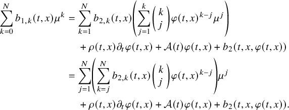 $$ \begin{align*}\begin{aligned} \sum_{k=0}^Nb_{1,k}(t,x)\mu^k &=\sum_{k=1}^Nb_{2,k}(t,x)\left(\sum_{j=1}^k\left(\begin{array}{l}k\\ j\end{array}\right)\varphi(t,x)^{k-j}\mu^j\right) \\ &\quad \, +\rho(t,x) \partial_t \varphi(t,x)+\mathcal A(t) \varphi(t,x)+b_2(t,x,\varphi(t,x))\\ &=\sum_{j=1}^N\left(\sum_{k=j}^Nb_{2,k}(t,x)\left(\begin{array}{l}k\\ j\end{array}\right)\varphi(t,x)^{k-j}\right)\mu^j \\ &\quad \, +\rho(t,x) \partial_t \varphi(t,x)+\mathcal A(t) \varphi(t,x)+b_2(t,x,\varphi(t,x)).\end{aligned}\end{align*} $$
It follows that
 $$ \begin{align} b_{1,j}(t,x)=\sum_{k=j}^Nb_{2,k}(t,x)\left(\begin{array}{l}k\\ j\end{array}\right)\varphi(t,x)^{k-j},\quad (t,x)\in Q,\ j=1,\ldots,N, \end{align} $$
and
 $$ \begin{align} b_{1,0}(t,x)-b_{2,0}(t,x) =\rho(t,x) \partial_t \varphi(t,x)+\mathcal A(t) \varphi(t,x)+b_2(t,x,\varphi(t,x))-b_2(t,x,0), \end{align} $$
for $(t,x)\in Q$
.
$(t,x)\in Q$
.
Applying (7.4) with $j=N$
and
$j=N$
and $j=N-1$
, we obtain
$j=N-1$
, we obtain
 $$ \begin{align} b_{1,N}=b_{2,N},\quad b_{1,N-1}=b_{2,N}\varphi+b_{2,N-1}. \end{align} $$
Moreover, the fact that the condition (2.16) holds true on the dense set J combined with the fact that $b_{j,k}\in C([0,T]\times \overline {\Omega })$
,
$b_{j,k}\in C([0,T]\times \overline {\Omega })$
, $j=1,2$
and
$j=1,2$
and $k=N-1,N$
implies that
$k=N-1,N$
implies that
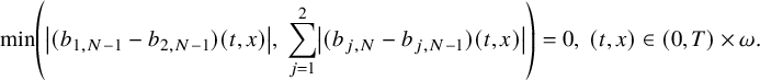 $$ \begin{align*} \min \left(\left|(b_{1,N-1}-b_{2,N-1})(t,x)\right|, \ \sum_{j=1}^2\left|(b_{j,N}-b_{j,N-1})(t,x)\right|\right)=0,\ (t,x)\in (0,T)\times\omega. \end{align*} $$
This condition implies that for all $(t,x)\in (0,T)\times \omega $
, we have either
$(t,x)\in (0,T)\times \omega $
, we have either $b_{2,N-1}(t,x)=b_{1,N-1}(t,x)$
or
$b_{2,N-1}(t,x)=b_{1,N-1}(t,x)$
or $b_{j,N}(t,x)=b_{j,N-1}(t,x)$
,
$b_{j,N}(t,x)=b_{j,N-1}(t,x)$
, $j=1,2$
. Combining this with (7.6) and the assumption that
$j=1,2$
. Combining this with (7.6) and the assumption that $|b_{1,N}(t,x)|>0$
for
$|b_{1,N}(t,x)|>0$
for $(t,x)\in J$
, we deduce that
$(t,x)\in J$
, we deduce that $\varphi =0$
on
$\varphi =0$
on $(0,T)\times \omega $
. Thus, (7.5) implies
$(0,T)\times \omega $
. Thus, (7.5) implies
 $$ \begin{align*}\left(b_{1,0}-b_{2,0}\right)(t,x)=\rho \partial_t \varphi(t,x)+\mathcal A(t) \varphi(t,x)+b_2(t,x,\varphi(t,x))-b_2(t,x,0)=0,\end{align*} $$
for $(t,x)\in (0,T)\times \omega $
. Finally, the assumption (2.18) implies that
$(t,x)\in (0,T)\times \omega $
. Finally, the assumption (2.18) implies that $b_{1,0}=b_{2,0}$
everywhere on Q. Thus,
$b_{1,0}=b_{2,0}$
everywhere on Q. Thus, $\varphi $
satisfies (7.2) with
$\varphi $
satisfies (7.2) with
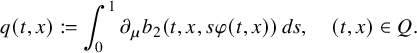 $$ \begin{align*}q(t,x):=\int_0^1\partial_\mu b_2(t,x,s\varphi(t,x))\, ds,\quad (t,x)\in Q.\end{align*} $$
Therefore, the uniqueness of solutions of (7.2) implies that $\varphi \equiv 0$
, and it follows that
$\varphi \equiv 0$
, and it follows that $b_1=b_2$
. The last statement of the theorem can be proved with similar arguments.
$b_1=b_2$
. The last statement of the theorem can be proved with similar arguments.
Proof of Theorem 2.4.
We assume that the conditions of Theorem 2.1 and (2.4) are fulfilled. We start by showing that $\partial _\mu h_1=\partial _\mu h_2$
. For this purpose, combining (1.6) and (7.1) with (2.20), we obtain
$\partial _\mu h_1=\partial _\mu h_2$
. For this purpose, combining (1.6) and (7.1) with (2.20), we obtain
 $$ \begin{align*}b_{1,1}(t,x)h_1(t,\mu)+b_{1,0}(t,x)=b_{2,1}(t,x)h_2(t,\mu)+b_{2,0}(t,x)+\mathcal A(t) \varphi(t,x),\quad (t,x,\mu)\in\Sigma\times{\mathbb R}.\end{align*} $$
Differentiating both sides of this identity with respect to $\mu $
, we get
$\mu $
, we get
 $$ \begin{align*}b_{1,1}(t,x)\partial_\mu h_1(t,\mu)=b_{2,1}(t,x)\partial_\mu h_2(t,\mu) ,\quad (t,x,\mu)\in\Sigma\times{\mathbb R},\end{align*} $$
and (2.23) implies that
 $$ \begin{align*}b_{1,1}(t,x_t)(\partial_\mu h_1(t,\mu)-\partial_\mu h_2(t,\mu))=0 ,\quad (t,\mu)\in(0,T)\times{\mathbb R},\end{align*} $$
with $b_{1,1}(t,x_t)\neq 0$
,
$b_{1,1}(t,x_t)\neq 0$
, $t\in (0,T)$
. It follows that
$t\in (0,T)$
. It follows that $\partial _\mu h_1=\partial _\mu h_2$
.
$\partial _\mu h_1=\partial _\mu h_2$
.
Now let us show that the function $\varphi $
of (7.1) is identically zero. Fixing
$\varphi $
of (7.1) is identically zero. Fixing $t\in (0,T)$
and applying the derivative at order
$t\in (0,T)$
and applying the derivative at order $n_t$
with respect to
$n_t$
with respect to $\mu $
on both sides of (7.1), we get
$\mu $
on both sides of (7.1), we get
 $$ \begin{align*}b_{1,1}(t,x)\partial_\mu^{n_t} h_1(t,\mu)=b_{2,1}(t,x)\partial_\mu^{n_t} h_2(t,\mu+\varphi(t,x))=b_{2,1}(t,x)\partial_\mu^{n_t} h_1(t,\mu+\varphi(t,x)) ,\end{align*} $$
for $(x,\mu )\in \Omega \times {\mathbb R}$
. Fixing
$(x,\mu )\in \Omega \times {\mathbb R}$
. Fixing $\mu =\mu _t-\varphi (t,x)$
and applying (2.21), we get
$\mu =\mu _t-\varphi (t,x)$
and applying (2.21), we get
 $$ \begin{align*}b_{1,1}(t,x)\partial_\mu^{n_t} h_1(t,\mu_t-\varphi(t,x))=b_{2,1}(t,x)\partial_\mu^{n_t} h_1(t,\mu_t)=0 ,\quad x\in \Omega,\end{align*} $$
and (2.22) implies
 $$ \begin{align*}\partial_\mu^{n_t} h_1(t,\mu_t-\varphi(t,x))=0 ,\quad x\in \Omega.\end{align*} $$
However, since ${\mathbb R}\ni \mu \mapsto \partial _\mu ^{n_t} h_1(t,\mu )$
is analytic, either it is uniformly vanishing or its zeros are isolated. By (2.21), we have that
${\mathbb R}\ni \mu \mapsto \partial _\mu ^{n_t} h_1(t,\mu )$
is analytic, either it is uniformly vanishing or its zeros are isolated. By (2.21), we have that $\partial _\mu ^{n_t} h_1(t,\,\cdot \,)\not \equiv 0$
for
$\partial _\mu ^{n_t} h_1(t,\,\cdot \,)\not \equiv 0$
for $t\in (0,T)$
. Thus, the zeros of
$t\in (0,T)$
. Thus, the zeros of ${\mathbb R}\ni \mu \mapsto \partial _\mu ^{n_t} h_1(t,\mu )$
are isolated. Using the fact that
${\mathbb R}\ni \mu \mapsto \partial _\mu ^{n_t} h_1(t,\mu )$
are isolated. Using the fact that $\overline {\Omega }\ni x\mapsto \varphi (t,x)$
is continuous, we deduce that the map
$\overline {\Omega }\ni x\mapsto \varphi (t,x)$
is continuous, we deduce that the map $\overline {\Omega }\ni x\mapsto \varphi (t,x)$
is constant. Then, recalling that
$\overline {\Omega }\ni x\mapsto \varphi (t,x)$
is constant. Then, recalling that $\varphi (t,x)=0$
for
$\varphi (t,x)=0$
for $x\in \partial \Omega $
, we deduce that
$x\in \partial \Omega $
, we deduce that $\varphi (t,\,\cdot \,)\equiv 0$
. Since here
$\varphi (t,\,\cdot \,)\equiv 0$
. Since here $t\in (0,T)$
is arbitrary chosen, we deduce that
$t\in (0,T)$
is arbitrary chosen, we deduce that $\varphi \equiv 0$
, and it follows that
$\varphi \equiv 0$
, and it follows that $b_1=b_2$
. The last statement of the theorem can be proved with similar arguments.
$b_1=b_2$
. The last statement of the theorem can be proved with similar arguments.
Proof of Theorem 2.5.
We will only consider the other statement of the theorem since the last statement can be deduced from similar arguments. Namely, we will prove that (2.4) and the conditions of Theorem 2.1 imply that $b_1=b_2$
. We start by showing that
$b_1=b_2$
. We start by showing that $\partial _\mu h_1=\partial _\mu h_2$
. For this purpose, combining (1.6) and (7.1) with (2.24), we obtain
$\partial _\mu h_1=\partial _\mu h_2$
. For this purpose, combining (1.6) and (7.1) with (2.24), we obtain
 $$ \begin{align*}b_{1,1}(t,x)h_1(t,b_{1,2}(t,x)\mu)+b_{1,0}(t,x)=b_{2,1}(t,x)h_2(t,b_{2,2}(t,x)\mu)+b_{2,0}(t,x)+\mathcal A(t) \varphi(t,x),\end{align*} $$
for $(t,x,\mu )\in \Sigma \times {\mathbb R}$
. Differentiating both sides of this identity with respect to
$(t,x,\mu )\in \Sigma \times {\mathbb R}$
. Differentiating both sides of this identity with respect to $\mu $
, we get
$\mu $
, we get
 $$ \begin{align*}b_{1,2}(t,x)b_{1,1}(t,x)\partial_\mu h_1(t,b_{1,2}(t,x)\mu)=b_{2,2}(t,x)b_{2,1}(t,x)\partial_\mu h_2(t,b_{2,2}(t,x)\mu) ,\quad (t,x,\mu)\in\Sigma\times{\mathbb R},\end{align*} $$
and (2.27) implies that
 $$ \begin{align*}b_{1,1}(t,x_t)b_{1,2}(t,x_t)(\partial_\mu h_1(t,b_{1,2}(t,x_t)\mu)-\partial_\mu h_2(t,b_{1,2}(t,x_t)\mu))=0 ,\quad (t,\mu)\in(0,T)\times{\mathbb R},\end{align*} $$
with $b_{1,1}(t,x_t)\neq 0$
and
$b_{1,1}(t,x_t)\neq 0$
and $b_{1,2}(t,x_t)\neq 0$
,
$b_{1,2}(t,x_t)\neq 0$
, $t\in (0,T)$
. It follows that
$t\in (0,T)$
. It follows that $\partial _\mu h_1=\partial _\mu h_2$
.
$\partial _\mu h_1=\partial _\mu h_2$
.
Now let us show that the function $\varphi $
of (7.1) is identically zero. Fixing
$\varphi $
of (7.1) is identically zero. Fixing $t\in (0,T)$
and applying the derivative at order
$t\in (0,T)$
and applying the derivative at order $n_t$
with respect to
$n_t$
with respect to $\mu $
on both sides of (7.1), we get
$\mu $
on both sides of (7.1), we get
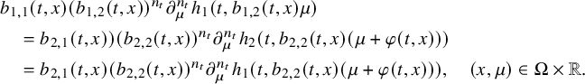 $$ \begin{align*}\begin{aligned} & b_{1,1}(t,x)(b_{1,2}(t,x))^{n_t}\partial_\mu^{n_t} h_1(t,b_{1,2}(t,x)\mu)\\ &\quad = b_{2,1}(t,x))(b_{2,2}(t,x))^{n_t}\partial_\mu^{n_t} h_2(t,b_{2,2}(t,x)(\mu+\varphi(t,x)))\\ &\quad = b_{2,1}(t,x)(b_{2,2}(t,x))^{n_t}\partial_\mu^{n_t} h_1(t,b_{2,2}(t,x)(\mu+\varphi(t,x))) ,\quad (x,\mu)\in \Omega\times{\mathbb R}.\end{aligned}\end{align*} $$
Fixing $\mu =-\varphi (t,x)$
and applying (2.27), we get
$\mu =-\varphi (t,x)$
and applying (2.27), we get
 $$ \begin{align*}b_{1,1}(t,x)(b_{1,2}(t,x))^{n_t}\partial_\mu^{n_t} h_1(t,-b_{1,2}(t,x)\varphi(t,x))=b_{2,1}(t,x)(b_{2,2}(t,x))^{n_t}\partial_\mu^{n_t} h_1(t,0)=0 ,\quad x\in \Omega,\end{align*} $$
and (2.26) implies
 $$ \begin{align*}\partial_\mu^{n_t} h_1(t,-b_{1,2}(t,x)\varphi(t,x)))=0 ,\quad x\in \Omega.\end{align*} $$
However, in view of (2.25), since ${\mathbb R}\ni \mu \mapsto \partial _\mu ^{n_t} h_1(t,\mu )$
is analytic,
${\mathbb R}\ni \mu \mapsto \partial _\mu ^{n_t} h_1(t,\mu )$
is analytic, $\partial _\mu ^{n_t} h_1(t,\,\cdot \,)\not \equiv 0$
and
$\partial _\mu ^{n_t} h_1(t,\,\cdot \,)\not \equiv 0$
and $\overline {\Omega }\ni x\mapsto b_{1,2}(t,x)\varphi (t,x)$
is continuous, we deduce that the map
$\overline {\Omega }\ni x\mapsto b_{1,2}(t,x)\varphi (t,x)$
is continuous, we deduce that the map $\overline {\Omega }\ni x\mapsto b_{1,2}(t,x)\varphi (t,x)$
is constant. Then, recalling that
$\overline {\Omega }\ni x\mapsto b_{1,2}(t,x)\varphi (t,x)$
is constant. Then, recalling that $\varphi (t,x)=0$
for
$\varphi (t,x)=0$
for $x\in \partial \Omega $
and applying (2.26), we deduce that
$x\in \partial \Omega $
and applying (2.26), we deduce that $\varphi (t,\,\cdot \,)\equiv 0$
. Since here
$\varphi (t,\,\cdot \,)\equiv 0$
. Since here $t\in (0,T)$
is arbitrary chosen, we deduce that
$t\in (0,T)$
is arbitrary chosen, we deduce that $\varphi \equiv 0$
, and it follows that
$\varphi \equiv 0$
, and it follows that $b_1=b_2$
.
$b_1=b_2$
.
Proof of Corollary 2.3.
Again, we will only consider the first statement of the corollary as the other statement follows similarly. Namely, we will prove that (2.4) and the conditions of Theorem 2.1 imply that $b_1=b_2$
. For this purpose, we only need to prove that the function
$b_1=b_2$
. For this purpose, we only need to prove that the function $\varphi $
of (7.1) is identically zero. We start by assuming that condition (i) is fulfilled. Fixing
$\varphi $
of (7.1) is identically zero. We start by assuming that condition (i) is fulfilled. Fixing $x\in \Omega $
and applying the derivative at order
$x\in \Omega $
and applying the derivative at order $n_x$
with respect to
$n_x$
with respect to $\mu $
on both sides of (7.1), we get
$\mu $
on both sides of (7.1), we get
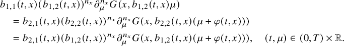 $$ \begin{align*}\begin{aligned} & b_{1,1}(t,x)(b_{1,2}(t,x))^{n_x}\partial_\mu^{n_x} G(x,b_{1,2}(t,x)\mu)\\ &\quad = b_{2,1}(t,x)(b_{2,2}(t,x))^{n_x}\partial_\mu^{n_x} G(x,b_{2,2}(t,x)(\mu+\varphi(t,x)))\\ &\quad = b_{2,1}(t,x)(b_{1,2}(t,x))^{n_x}\partial_\mu^{n_x} G(x,b_{1,2}(t,x)(\mu+\varphi(t,x))) ,\quad (t,\mu)\in (0,T)\times{\mathbb R}.\end{aligned}\end{align*} $$
Applying (2.26), fixing $\mu =\frac {\mu _x}{b_{1,2}(t,x)}-\varphi (t,x)$
and using (2.30), we get
$\mu =\frac {\mu _x}{b_{1,2}(t,x)}-\varphi (t,x)$
and using (2.30), we get
 $$ \begin{align*}b_{1,1}(t,x)(b_{1,2}(t,x))^{n_x}\partial_\mu^{n_x} G(x,\mu_x-b_{1,2}(t,x)\varphi(t,x))=b_{2,1}(t,x)(b_{1,2}(t,x))^{n_x}\partial_\mu^{n_x} G(x,\mu_x)=0 ,\end{align*} $$
for $t\in (0,T)$
. Then, (2.26) implies
$t\in (0,T)$
. Then, (2.26) implies
 $$ \begin{align*}\partial_\mu^{n_x} G(x,\mu_x-b_{1,2}(t,x)\varphi(t,x))=0 ,\quad t\in (0,T).\end{align*} $$
However, since ${\mathbb R}\ni \mu \mapsto \partial _\mu ^{n_x} G(x,\mu )$
is analytic and
${\mathbb R}\ni \mu \mapsto \partial _\mu ^{n_x} G(x,\mu )$
is analytic and $[0,T]\ni t\mapsto b_{1,2}(t,x)\varphi (t,x)$
is continuous, we deduce that either
$[0,T]\ni t\mapsto b_{1,2}(t,x)\varphi (t,x)$
is continuous, we deduce that either $\partial _\mu ^{n_x} G(x,\,\cdot \,)\equiv 0$
or that the map
$\partial _\mu ^{n_x} G(x,\,\cdot \,)\equiv 0$
or that the map $[0,T]\ni t\mapsto b_{1,2}(t,x)\varphi (t,x)$
is constant. Since
$[0,T]\ni t\mapsto b_{1,2}(t,x)\varphi (t,x)$
is constant. Since $\partial _\mu ^{n_x} G(x,\,\cdot \,)\not \equiv 0$
, we deduce that the map
$\partial _\mu ^{n_x} G(x,\,\cdot \,)\not \equiv 0$
, we deduce that the map $[0,T]\ni t\mapsto b_{1,2}(t,x)\varphi (t,x)$
is constant. Then, recalling that
$[0,T]\ni t\mapsto b_{1,2}(t,x)\varphi (t,x)$
is constant. Then, recalling that $\varphi (0,\,\cdot \,)=0$
and applying (2.26), we deduce that, for all
$\varphi (0,\,\cdot \,)=0$
and applying (2.26), we deduce that, for all $t\in [0,T]$
,
$t\in [0,T]$
, $\varphi (t,x)=0$
. Since here
$\varphi (t,x)=0$
. Since here $x\in \Omega $
is arbitrary chosen, we deduce that
$x\in \Omega $
is arbitrary chosen, we deduce that $\varphi \equiv 0$
, and it follows that
$\varphi \equiv 0$
, and it follows that $b_1=b_2$
.
$b_1=b_2$
.
Combining the above argumentation and the arguments used for the proof of Theorem 2.5, one can easily check that (2.4) implies also that $b_1=b_2$
when condition (ii) is fulfilled. This completes the proof of the corollary.
$b_1=b_2$
when condition (ii) is fulfilled. This completes the proof of the corollary.
Proofs of Corollary 2.4.
With the conclusion of Theorem 2.2 at hand, combined with $b_j(t,x,\mu )=q_j(t,x)\mu $
for
$b_j(t,x,\mu )=q_j(t,x)\mu $
for $(t,x,\mu )\in Q\times {\mathbb R}$
and
$(t,x,\mu )\in Q\times {\mathbb R}$
and $j=1,2$
, both (2.5) and (2.9) yield that
$j=1,2$
, both (2.5) and (2.9) yield that
 $$ \begin{align} q_1(x,t)\mu=S_\varphi (q_2(x,t)\mu) =q_2(t,x)(\mu+\varphi(t,x))+\rho(t,x) \partial_t \varphi(t,x)+\mathcal A(t) \varphi(t,x), \end{align} $$
for any $(t,x,\mu )\in Q\times {\mathbb R}$
. In particular, plugging
$(t,x,\mu )\in Q\times {\mathbb R}$
. In particular, plugging $\mu =0$
into (7.7), the function
$\mu =0$
into (7.7), the function $\varphi $
satisfies the IBVP
$\varphi $
satisfies the IBVP
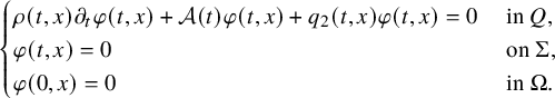 $$ \begin{align*} \begin{cases} \rho(t,x) \partial_t \varphi(t,x)+\mathcal A(t) \varphi(t,x)+q_2(t,x)\varphi(t,x)=0 & \text{ in }Q, \\ \varphi(t,x)=0 & \text{ on }\Sigma,\\ \varphi(0,x)=0 & \text{ in }\Omega. \end{cases} \end{align*} $$
By the uniqueness of the above IBVP, we must have $\varphi \equiv 0$
in Q. Now, by using (7.7) again, we have
$\varphi \equiv 0$
in Q. Now, by using (7.7) again, we have $q_1(t,x)\mu =q_2(t,x)\mu $
, for all
$q_1(t,x)\mu =q_2(t,x)\mu $
, for all $\mu \in {\mathbb R}$
, which implies
$\mu \in {\mathbb R}$
, which implies $q_1=q_2$
as desired. This completes the proof.
$q_1=q_2$
as desired. This completes the proof.
8 Application to the simultaneous determination of nonlinear and source terms
One of the important application of our results is to inverse source problems, where the aim is to recover both the source and nonlinear terms simultaneously. In this section, we consider the IBVP
 $$ \begin{align} \begin{cases} \rho(t,x) \partial_t u(t,x)+\mathcal A(t) u(t,x)+ d(t,x,u(t,x)) = F(t,x) & \text{ in } Q,\\ u(t,x) = f(t,x) & \text{ on } \Sigma, \\ u(0,x) = 0 & \text{ for }x \in \Omega, \end{cases} \end{align} $$
with $d\in \mathbb A({\mathbb R};C^{\frac {\alpha }{2},\alpha }([0,T]\times \overline {\Omega }))$
and
$d\in \mathbb A({\mathbb R};C^{\frac {\alpha }{2},\alpha }([0,T]\times \overline {\Omega }))$
and $F\in C^{\frac {\alpha }{2},\alpha }([0,T]\times \overline {\Omega })$
satisfying the conditions
$F\in C^{\frac {\alpha }{2},\alpha }([0,T]\times \overline {\Omega })$
satisfying the conditions
 $$ \begin{align} F(0,x)=0,\quad x\in\partial\Omega, \end{align} $$
 $$ \begin{align} d(t,x,0)=0,\quad (t,x)\in Q. \end{align} $$
The latter condition is just for presentational purposes and can be removed by redefining F. In a similar way to the problem studied above, we assume here that there exists $f=f_0\in \mathcal K_0$
such that (8.1) admits a unique solution for
$f=f_0\in \mathcal K_0$
such that (8.1) admits a unique solution for $f=f_0$
. Then, applying Proposition 3.1, we can prove that there exists
$f=f_0$
. Then, applying Proposition 3.1, we can prove that there exists $\epsilon>0$
, depending on a,
$\epsilon>0$
, depending on a, $\rho $
, d, F,
$\rho $
, d, F, $f_0$
,
$f_0$
, $\Omega $
, T, such that, for all
$\Omega $
, T, such that, for all $f\in \mathbb B(f_0,\epsilon )$
, (8.1) admits a unique solution
$f\in \mathbb B(f_0,\epsilon )$
, (8.1) admits a unique solution $u_f\in C^{1+\frac {\alpha }{2},2+\alpha }([0,T]\times \overline {\Omega })$
that lies in a sufficiently small neighborhood of the solution
$u_f\in C^{1+\frac {\alpha }{2},2+\alpha }([0,T]\times \overline {\Omega })$
that lies in a sufficiently small neighborhood of the solution $u_0$
of (8.1) when
$u_0$
of (8.1) when $f=f_0$
. Using these properties, we can define the parabolic DN map
$f=f_0$
. Using these properties, we can define the parabolic DN map
 $$ \begin{align*}\mathcal M_{(d,F)}:\mathbb B(f_0,\epsilon)\ni f\mapsto \left. \partial_{\nu(a)} u(t,x)\right|{}_{\Sigma},\end{align*} $$
where u solves (8.1).
We consider in this section the inverse problem of determining simultaneously the nonlinear term d and the source term F appearing in (8.1). Similarly to the problem (IP), there will be a gauge invariance for this inverse problem. Indeed, fix $\varphi \in C^{1+\frac {\alpha }{2},2+\alpha }([0,T]\times \overline {\Omega })$
satisfying (1.6) and consider the map
$\varphi \in C^{1+\frac {\alpha }{2},2+\alpha }([0,T]\times \overline {\Omega })$
satisfying (1.6) and consider the map $U_\varphi $
mapping
$U_\varphi $
mapping $ C^\infty ({\mathbb R};C^{\frac {\alpha }{2},\alpha }([0,T]\times \overline {\Omega }))\times C^{\frac {\alpha }{2},\alpha }([0,T]\times \overline {\Omega })$
into itself and defined by
$ C^\infty ({\mathbb R};C^{\frac {\alpha }{2},\alpha }([0,T]\times \overline {\Omega }))\times C^{\frac {\alpha }{2},\alpha }([0,T]\times \overline {\Omega })$
into itself and defined by $U_\varphi (d,F)=(d_\varphi ,F_\varphi )$
with
$U_\varphi (d,F)=(d_\varphi ,F_\varphi )$
with
 $$ \begin{align} \begin{split} d_\varphi(t,x,\mu)&=d(t,x,\mu+\varphi(t,x))-d(t,x,\varphi(t,x)),\\ F_\varphi(t,x)&=F(t,x)-\rho(t,x) \partial_t \varphi(t,x)-\mathcal A(t) \varphi(t,x)- d(t,x,\varphi(t,x)), \end{split} \end{align} $$
for $ (t,x,\mu )\in Q\times {\mathbb R}$
. Then, one can easily check that
$ (t,x,\mu )\in Q\times {\mathbb R}$
. Then, one can easily check that $\mathcal M_{(d,F)}=\mathcal M_{U_\varphi (d,F)}$
. Note that (8.4) is equivalent to (1.7) for
$\mathcal M_{(d,F)}=\mathcal M_{U_\varphi (d,F)}$
. Note that (8.4) is equivalent to (1.7) for
 $$ \begin{align*}b(t,x,\mu)=d(t,x,\mu)-F(t,x),\quad (t,x,\mu)\in Q\times{\mathbb R}.\end{align*} $$
Following, this property, in general, the best one can expect for our inverse problem is the determination of $U_\varphi (d,F)$
from
$U_\varphi (d,F)$
from $\mathcal M_{(d,F)}$
for some
$\mathcal M_{(d,F)}$
for some $\varphi \in C^{1+\frac {\alpha }{2},2+\alpha }([0,T]\times \overline {\Omega })$
satisfying (1.6). Our first result will be stated in that sense.
$\varphi \in C^{1+\frac {\alpha }{2},2+\alpha }([0,T]\times \overline {\Omega })$
satisfying (1.6). Our first result will be stated in that sense.
Proposition 8.1. Let $a:=(a_{ik})_{1 \leqslant i,k \leqslant n} \in C^\infty ([0,T]\times \overline {\Omega };{\mathbb R}^{n \times n})$
satisfy (1.1),
$a:=(a_{ik})_{1 \leqslant i,k \leqslant n} \in C^\infty ([0,T]\times \overline {\Omega };{\mathbb R}^{n \times n})$
satisfy (1.1), $\rho \in C^\infty ([0,T]\times \overline {\Omega };{\mathbb R}_+)$
and, for
$\rho \in C^\infty ([0,T]\times \overline {\Omega };{\mathbb R}_+)$
and, for $j=1,2$
, let
$j=1,2$
, let $d_j\in \mathbb A({\mathbb R};C^{\frac {\alpha }{2},\alpha }([0,T]\times \overline {\Omega }))\cap C^\infty ([0,T]\times \overline {\Omega }\times {\mathbb R})$
and
$d_j\in \mathbb A({\mathbb R};C^{\frac {\alpha }{2},\alpha }([0,T]\times \overline {\Omega }))\cap C^\infty ([0,T]\times \overline {\Omega }\times {\mathbb R})$
and $F_j\in C^\infty ([0,T]\times \overline {\Omega })$
satisfy (8.2)–(8.3) with
$F_j\in C^\infty ([0,T]\times \overline {\Omega })$
satisfy (8.2)–(8.3) with $d=d_j$
and
$d=d_j$
and $F=F_j$
. We assume also that there exists
$F=F_j$
. We assume also that there exists $f_0\in \mathcal K_0$
such that problem (8.1), with
$f_0\in \mathcal K_0$
such that problem (8.1), with $f=f_0$
and
$f=f_0$
and $d=d_j$
,
$d=d_j$
, $F=F_j$
,
$F=F_j$
, $j=1,2$
, is well-posed. Then, the condition
$j=1,2$
, is well-posed. Then, the condition
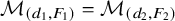 $$ \begin{align} \mathcal M_{(d_1,F_1)}=\mathcal M_{(d_2,F_2)} \end{align} $$
implies that there exists $\varphi \in C^{1+\frac {\alpha }{2},2+\alpha }([0,T]\times \overline {\Omega })$
satisfying (1.6) such that
$\varphi \in C^{1+\frac {\alpha }{2},2+\alpha }([0,T]\times \overline {\Omega })$
satisfying (1.6) such that
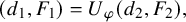 $$ \begin{align} (d_1,F_1)=U_\varphi(d_2,F_2), \end{align} $$
where $U_\varphi $
is the map defined by (8.4).
$U_\varphi $
is the map defined by (8.4).
Proof. Fixing
 $$ \begin{align*}b_j(t,x,\mu)=d_j(t,x,\mu)-F_j(t,x),\quad (t,x,\mu)\in Q\times{\mathbb R},\end{align*} $$
one can check that $\mathcal N_{b_j}=\mathcal M_{(d_j,F_j)}$
and (8.5) implies (2.4). Then, applying Theorem 2.1, we deduce that (2.5) holds true which clearly implies (8.6).
$\mathcal N_{b_j}=\mathcal M_{(d_j,F_j)}$
and (8.5) implies (2.4). Then, applying Theorem 2.1, we deduce that (2.5) holds true which clearly implies (8.6).
It is well known that when $\mu \mapsto d(t,x,\mu )$
is linear,
$\mu \mapsto d(t,x,\mu )$
is linear, $(t,x)\in Q$
, there is no hope to determine general class of source terms
$(t,x)\in Q$
, there is no hope to determine general class of source terms $F\in C^\infty ([0,T]\times \overline {\Omega })$
satisfying the condition of Proposition 8.1 from the knowledge of the map
$F\in C^\infty ([0,T]\times \overline {\Omega })$
satisfying the condition of Proposition 8.1 from the knowledge of the map $\mathcal M_{(d,F)}$
; see Example 1.1 or, for example, [Reference Kian, Soccorsi, Xue and YamamotoKSXY22, Appendix A]. Nevertheless, this invariance breaks for several classes of nonlinear terms d for which we can prove the simultaneous determination of d and F from
$\mathcal M_{(d,F)}$
; see Example 1.1 or, for example, [Reference Kian, Soccorsi, Xue and YamamotoKSXY22, Appendix A]. Nevertheless, this invariance breaks for several classes of nonlinear terms d for which we can prove the simultaneous determination of d and F from $\mathcal M_{(d,F)}$
. More precisely, applying Corollary 2.1 and Theorems 2.3, 2.4, 2.5, we can show the following.
$\mathcal M_{(d,F)}$
. More precisely, applying Corollary 2.1 and Theorems 2.3, 2.4, 2.5, we can show the following.
Corollary 8.1. Let the condition of Proposition 8.1 be fulfilled, and assume that, for $j=1,2$
, the nonlinear term
$j=1,2$
, the nonlinear term $d_j$
satisfies one of the following conditions:
$d_j$
satisfies one of the following conditions:
-
(i) There exists
$\kappa \in C^{\frac {\alpha }{2},\alpha }([0,T]\times \overline {\Omega })$
such that
$$ \begin{align*}d_1(t,x,\kappa(t,x))-d_2(t,x,\kappa(t,x))=F_1(t,x)-F_2(t,x),\quad (t,x)\in [0,T]\times\overline{\Omega}.\end{align*} $$
-
(ii) There exists
$N_j\geqslant 2$
such that
$$ \begin{align*}d_j(t,x,\mu)=\sum_{k=1}^{N_j} d_{j,k}(t,x)\mu^k,\quad (t,x,\mu)\in[0,T]\times\overline{\Omega}\times{\mathbb R},\ j=1,2.\end{align*} $$
Moreover, for
$N=\min (N_1,N_2)$
and J a dense subset of Q, we have
$$ \begin{align*}\min \left(|(d_{1,N-1}-d_{2,N-1})(t,x)|,\, \sum_{j=1}^2|(d_{j,N}-d_{j,N-1})(t,x)|\right)=0,\ (t,x)\in J,\end{align*} $$
$$ \begin{align*}d_{1,N}(t,x)\neq0,\quad (t,x)\in J.\end{align*} $$
-
(iii) There exists
$h_j\in \mathbb A({\mathbb R};C^{\frac {\alpha }{2}}([0,T]))$
such that
$$ \begin{align*}d_j(t,x,\mu)=q_{j}(t,x)h_j(t,\mu),\quad (t,x,\mu)\in[0,T]\times\overline{\Omega}\times{\mathbb R},\ j=1,2.\end{align*} $$
Assume also that, for all
$t\in (0,T)$
, there exist
$\mu _t\in {\mathbb R}$
and
$n_t\in \mathbb N$
such that
$$ \begin{align*}\partial_\mu^{n_t} h_1(t,\,\cdot\,)\not\equiv0,\quad\partial_\mu^{n_t} h_1(t,\mu_t)=0,\quad t\in(0,T).\end{align*} $$
Moreover, we assume that
and that for all
$$ \begin{align*}q_{1}(t,x)\neq0,\quad (t,x)\in Q,\end{align*} $$
$t\in (0,T)$
, there exists
$x_t\in \partial \Omega $
such that
$$ \begin{align*}q_{1}(t,x_t)=q_{2}(t,x_t)\neq0,\quad t\in(0,T).\end{align*} $$
-
(iv) There exists
$h_j(t,\cdot )\in \mathbb A({\mathbb R};C^{\frac {\alpha }{2}}([0,T]))$
such that
$$ \begin{align*}d_j(t,x,\mu)=q_{j,1}(t,x)h_j(t,q_{j,2}(t,x)\mu),\quad (t,x,\mu)\in[0,T]\times\overline{\Omega}\times{\mathbb R},\ j=1,2.\end{align*} $$
Assume also that, for all
$t\in (0,T)$
, there exists
$n_t\in \mathbb N$
such that
$$ \begin{align*}\partial_\mu^{n_t} h_1(t,\,\cdot\,)\not\equiv0,\quad\partial_\mu^{n_t} h_1(t,0)=0,\quad t\in(0,T).\end{align*} $$
Moreover, we assume that
and that for all
$$ \begin{align*}q_{1,1}(t,x)\neq0,\quad q_{1,2}(t,x)\neq0\quad (t,x)\in Q,\end{align*} $$
$t\in (0,T)$
, there exists
$x_t\in \partial \Omega $
such that
$$ \begin{align*}q_{1,1}(t,x_t)=q_{2,1}(t,x_t)\neq0,\quad q_{1,2}(t,x_t)=q_{2,2}(t,x_t)\neq0,\quad t\in(0,T).\end{align*} $$


Then (8.5) implies that $d_1=d_2$
and
$d_1=d_2$
and $F_1=F_2$
.
$F_1=F_2$
.
Proof. Fixing
 $$ \begin{align*}b_j(t,x,\mu)=d_j(t,x,\mu)-F_j(t,x),\quad (t,x,\mu)\in Q\times{\mathbb R},\end{align*} $$
one can check that $\mathcal N_{b_j}=\mathcal M_{(d_j,F_j)}$
and (8.5) implies (2.4). Then, applying Corollary 2.1 and Theorem 2.3, 2.4, 2.5, we deduce that for semilinear terms
$\mathcal N_{b_j}=\mathcal M_{(d_j,F_j)}$
and (8.5) implies (2.4). Then, applying Corollary 2.1 and Theorem 2.3, 2.4, 2.5, we deduce that for semilinear terms $d_j$
satisfying one of the conditions (i), (ii), (iii), (iv), we have
$d_j$
satisfying one of the conditions (i), (ii), (iii), (iv), we have
 $$ \begin{align*}d_1(t,x,\mu)-F_1(t,x)=b_1(t,x,\mu)=b_2(t,x,\mu)=d_2(t,x,\mu)-F_2(t,x),\quad (t,x,\mu)\in Q\times{\mathbb R}.\end{align*} $$
Choosing $\mu =0$
in the above identity and applying (8.3), we deduce that
$\mu =0$
in the above identity and applying (8.3), we deduce that $F_1=F_2$
and then
$F_1=F_2$
and then $d_1=d_2$
.
$d_1=d_2$
.
A Carleman estimates
In the end of this paper, we prove the Carleman estimate in Section 6. For the sake of convenience, we also state the result as follows.
Lemma A.1. Let $n\geqslant 3$
,
$n\geqslant 3$
, $q\in L^\infty (Q)$
and
$q\in L^\infty (Q)$
and $v\in H^1(Q)\cap L^2(0,T;H^2(\Omega ))$
satisfy the condition
$v\in H^1(Q)\cap L^2(0,T;H^2(\Omega ))$
satisfy the condition
 $$ \begin{align} v|_{\Sigma}=0,\quad v|_{t=0}=0. \end{align} $$
Then, there exists $\tau _0>0$
depending on T,
$\tau _0>0$
depending on T, $\Omega $
and
$\Omega $
and $\left \lVert q\right \rVert _{L^\infty (Q)}$
such that for all
$\left \lVert q\right \rVert _{L^\infty (Q)}$
such that for all $\tau>\tau _0$
, the estimate
$\tau>\tau _0$
, the estimate
 $$ \begin{align} \begin{aligned} &\tau\int_0^T\int_{\Gamma_{+}(x_0)}e^{-2(\tau^2t+\tau\psi(x))}\left\lvert\partial_\nu v\right\rvert^2\left\lvert\partial_\nu\psi(x) \right\rvert d\sigma(x)dt+\tau^2\int_Qe^{-2(\tau^2t+\tau\psi(x))}\left\lvert v\right\rvert^2dxdt\\ &\quad \leqslant C\left(\int_Qe^{-2(\tau^2t+\tau\psi(x))}\left\lvert(\partial_t-\Delta_x+q)v\right\rvert^2\, dxdt \right. \\ &\qquad \left. +\,\tau\int_0^T\int_{\Gamma_{-}(x_0)}e^{-2(\tau^2t+\tau\psi(x))}\left\lvert\partial_\nu v\right\rvert^2\left\lvert\partial_\nu\psi(x) \right\rvert d\sigma(x)\, dt\right) \end{aligned}\end{align} $$
holds true.
Proof. Recall that $\psi (x)=|x-x_0|$
,
$\psi (x)=|x-x_0|$
, $x\in \Omega $
, for
$x\in \Omega $
, for $x_0\in {\mathbb R}^n\setminus \overline {\Omega }$
, then
$x_0\in {\mathbb R}^n\setminus \overline {\Omega }$
, then $\psi $
satisfies the eikonal equation
$\psi $
satisfies the eikonal equation $\left |\nabla _x \psi (x)\right |=1$
for
$\left |\nabla _x \psi (x)\right |=1$
for $x\in \Omega $
. Without loss of generality, we assume that u is real valued and
$x\in \Omega $
. Without loss of generality, we assume that u is real valued and $q=0$
. In order to prove the estimate (A.2), we fix
$q=0$
. In order to prove the estimate (A.2), we fix $v\in C^2(\overline {Q})$
satisfying (A.1),
$v\in C^2(\overline {Q})$
satisfying (A.1), $s>0$
, and we set
$s>0$
, and we set
 $$ \begin{align*}w=e^{-(\tau^2t+\tau\psi(x)-s\frac{\psi(x)^2}{2})}v \end{align*} $$
in such a way that
 $$ \begin{align}e^{-(\tau^2t+\tau\psi(x)-s\frac{\psi(x)^2}{2})}(\partial_t-\Delta_x) v=P_{\tau,s}w,\end{align} $$
where $P_{\tau ,s}$
is given by
$P_{\tau ,s}$
is given by
 $$ \begin{align*}P_{\tau,s}=\partial_t-\Delta +2s\tau\psi-\tau \Delta \psi+s\psi\Delta\psi-s^2\psi^2+s-2\tau\nabla\psi\cdot\nabla+2s\psi \nabla\psi\cdot\nabla.\end{align*} $$
Here, we used the fact that the function $\psi $
satisfies the eikonal equation.
$\psi $
satisfies the eikonal equation.
We next decompose $P_{\tau ,s}$
into two parts
$P_{\tau ,s}$
into two parts $P_{\tau ,s}=P_{\tau ,s,+}+P_{\tau ,s,-}$
with
$P_{\tau ,s}=P_{\tau ,s,+}+P_{\tau ,s,-}$
with
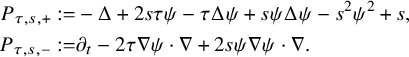 $$ \begin{align*} P_{\tau,s,+}:=&-\Delta +2s\tau\psi-\tau \Delta \psi +s\psi \Delta\psi-s^2\psi^2+s ,\\ P_{\tau,s,-}:=&\partial_t-2\tau\nabla\psi\cdot\nabla+2s\psi \nabla\psi\cdot\nabla. \end{align*} $$
Then, it follows that
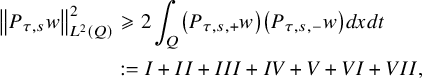 $$ \begin{align} \begin{aligned} \left\lVert P_{\tau,s}w\right\rVert_{L^2(Q)}^2 &\geqslant 2\int_Q \left( P_{\tau,s,+}w\right) \left( P_{\tau,s,-}w\right) dxdt\\ &:=I+II+III+IV+V+VI+VII, \end{aligned} \end{align} $$
where
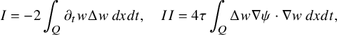 $$ \begin{align*}I=-2\int_Q\partial_tw\Delta w\, dxdt,\quad II=4\tau\int_Q\Delta w\nabla\psi\cdot\nabla w\, dxdt,\qquad\qquad \end{align*} $$
 $$ \begin{align*}III=4s\tau\int_Q\psi w \partial_tw \, dxdt,\quad IV=-8s\tau^2\int_Q\psi w\nabla\psi\cdot\nabla w\, dxdt, \qquad \end{align*} $$
 $$ \begin{align*}V=-4s \int_{Q} \Delta w \psi \nabla \psi \cdot \nabla w \, dxdt, \quad VI=8s^2 \tau\int_{Q} \psi^2 w\nabla \psi \cdot \nabla w \, dxdt, \end{align*} $$
and
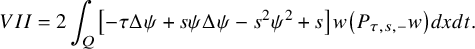 $$ \begin{align*}VII= 2\int_Q\left[-\tau\Delta \psi+s\psi\Delta\psi-s^2\psi^2+s\right]w \left( P_{\tau,s,-}w\right) dxdt.\end{align*} $$
Recalling that $w|_\Sigma =0$
and
$w|_\Sigma =0$
and $w|_{t=0}=0$
, fixing
$w|_{t=0}=0$
, fixing
 $$ \begin{align*}c_*=\inf_{x\in\Omega}\psi(x)>0\end{align*} $$
and integrating by parts, we find
 $$ \begin{align*} \begin{aligned} I &=2\int_Q\partial_t\nabla w\cdot\nabla w\, dxdt=\int_Q\partial_t|\nabla w|^2\, dxdt=\int_\Omega |\nabla w(T,x)|^2\, dx\geqslant0, \\ III &=2s\tau\int_Q\psi\partial_t(w^2)\, dxdt=2s\tau\int_\Omega \psi(x) w(T,x)^2\, dx\geqslant 2c_*s\tau\int_\Omega w(T,x)^2\, dx\geqslant0, \\ IV &=-4s\tau^2\int_Q(x-x_0)\cdot\nabla (w^2)\,dxdt =4s\tau^2\int_Q\textrm{div}(x-x_0) w^2\, dxdt\\ &=4ns\tau^2\int_Qw^2\, dxdt\geqslant0, \end{aligned} \end{align*} $$
and similarly,
 $$ \begin{align*}VI=-4s^2 \tau \int_{Q} \textrm{div}(\psi^2 \nabla \psi) w^2 \, dxdt = -4(n+1)s^2 \tau \int_Q |x-x_0| w^2 \, dxdt, \end{align*} $$
where we utilized the fact that $\psi ^2 \nabla \psi = |x-x_0|(x-x_0)$
.
$\psi ^2 \nabla \psi = |x-x_0|(x-x_0)$
.
Now, let us consider $II$
. Integrating by parts and using the fact that
$II$
. Integrating by parts and using the fact that $w|_\Sigma =0$
, we get
$w|_\Sigma =0$
, we get
 $$ \begin{align*}\begin{aligned}II &=4\tau\int_\Sigma \partial_\nu w\nabla\psi\cdot\nabla w\, d\sigma(x)dt-4\tau\int_Q\nabla w\cdot\nabla(\nabla\psi\cdot\nabla w)\, dxdt\\ &=4\tau\int_\Sigma (\partial_\nu w)^2\partial_\nu\psi \, d\sigma(x)dt-4\tau\int_Q D^2\psi(\nabla w,\nabla w)\, dxdt-2\tau \int_Q\nabla\psi\cdot\nabla (|\nabla w|^2)\, dxdt\\ &=2\tau\int_\Sigma (\partial_\nu w)^2\partial_\nu\psi \, d\sigma(x) dt-4\tau\int_Q D^2\psi(\nabla w,\nabla w)\, dxdt+2\tau \int_Q\Delta\psi|\nabla w|^2\, dxdt\\ &=2\tau\int_\Sigma (\partial_\nu w)^2\partial_\nu\psi \, d\sigma(x)dt-4\tau\int_Q D^2\psi(\nabla w,\nabla w)\, dxdt+2\tau \int_Q\frac{n-1}{|x-x_0|}|\nabla w|^2\, dxdt.\end{aligned}\end{align*} $$
However, one can check that
 $$ \begin{align*}D^2\psi(x)=|x-x_0|^{-3}\left(|x-x_0|^2\mathrm{Id}_{{\mathbb R}^{n\times n}}-N(x)\right),\quad x\in\Omega\end{align*} $$
with $N(x)= ((x_i-x_0^i)(x_j-x_0^j) )_{1\leqslant i,j\leqslant n}$
where
$N(x)= ((x_i-x_0^i)(x_j-x_0^j) )_{1\leqslant i,j\leqslant n}$
where $x=(x_1,\ldots ,x_n)$
and
$x=(x_1,\ldots ,x_n)$
and $x_0=(x_0^1,\ldots ,x_0^n)$
. Moreover, it can be proved that
$x_0=(x_0^1,\ldots ,x_0^n)$
. Moreover, it can be proved that $N(x)$
is a symmetric matrix whose eigenvalues are either
$N(x)$
is a symmetric matrix whose eigenvalues are either $0$
or
$0$
or $|x-x_0|^2$
. Thus, we get
$|x-x_0|^2$
. Thus, we get
 $$ \begin{align*}0\leqslant D^2\psi(x)(\nabla w(t,x),\nabla w(t,x))\leqslant \frac{|\nabla w(t,x)|^2}{|x-x_0|},\quad \text{ for }(t,x)\in Q,\end{align*} $$
and it follows that
 $$ \begin{align} \begin{aligned} II &\geqslant 2\tau\int_\Sigma (\partial_\nu w)^2\partial_\nu\psi \, d\sigma(x)dt+\tau \int_Q\frac{2(n-3)}{|x-x_0|}|\nabla w|^2\, dxdt\\ &\geqslant 2\tau\int_\Sigma (\partial_\nu w)^2\partial_\nu\psi \, d\sigma(x)dt+c_1(n-3)\tau \int_Q|\nabla w|^2\, dxdt, \end{aligned} \end{align} $$
where $c_1=\inf _{x\in \Omega }\frac {2}{|x-x_0|}$
.
$c_1=\inf _{x\in \Omega }\frac {2}{|x-x_0|}$
.
Applying similar computations for V, one has that
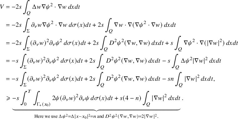 $$ \begin{align} \begin{aligned} V &=-2s \int_{Q} \Delta w \nabla \psi^2 \cdot \nabla w \, dxdt \\ &=-2s\int_\Sigma \partial_\nu w\nabla\psi^2\cdot\nabla w\, d\sigma(x)dt +2s\int_Q\nabla w\cdot\nabla(\nabla\psi^2\cdot\nabla w)\, dxdt\\ &=-2s\int_\Sigma (\partial_\nu w)^2\partial_\nu\psi^2 \, d\sigma(x)dt+2s\int_Q D^2\psi^2(\nabla w,\nabla w)\, dxdt +s\int_Q\nabla\psi^2\cdot\nabla (|\nabla w|^2)\, dxdt\\ &=-s\int_\Sigma (\partial_\nu w)^2\partial_\nu\psi^2 \, d\sigma(x) dt+2s\int_Q D^2\psi^2(\nabla w,\nabla w)\, dxdt- s \int_Q\Delta\psi^2|\nabla w|^2\, dxdt\\ &=-s\int_\Sigma (\partial_\nu w)^2\partial_\nu\psi^2 \, d\sigma(x)dt+2s\int_Q D^2\psi^2 (\nabla w,\nabla w)\, dxdt-sn\int_Q|\nabla w|^2\, dxdt,\\ &\geqslant \underbrace{-s\int_0^T\int_{\Gamma_{+}(x_0)} 2\psi(\partial_\nu w)^2\partial_\nu\psi \, d\sigma(x)dt+s(4-n)\int_Q|\nabla w|^2\, dxdt}_{\text{Here we use }\Delta \psi^2 = \Delta |x-x_0|^2 =n \text{ and }D^2\psi^2(\nabla w, \nabla w) = 2 |\nabla w|^2.}. \end{aligned} \end{align} $$
In addition, the sum of the last two terms on the right-hand side of (A.5) and (A.6) is
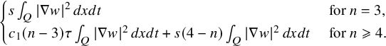 $$ \begin{align} \begin{cases} s\int_Q|\nabla w|^2\, dxdt &\text{ for }n=3,\\ c_1(n-3)\tau \int_Q|\nabla w|^2\, dxdt+s(4-n)\int_Q|\nabla w|^2\, dxdt & \text{ for }n\geqslant 4. \end{cases} \end{align} $$
By choosing $\tau \geqslant \frac {s(4-n)}{c_1(n-3)}$
for
$\tau \geqslant \frac {s(4-n)}{c_1(n-3)}$
for $n\geqslant 4$
, both cases appearing in (A.7) are nonnegative. Now fixing
$n\geqslant 4$
, both cases appearing in (A.7) are nonnegative. Now fixing $c_2=2\sup _{x\in \partial \Omega }\psi (x)$
, and choosing
$c_2=2\sup _{x\in \partial \Omega }\psi (x)$
, and choosing
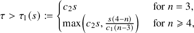 $$ \begin{align*} \tau>\tau_1(s):=\begin{cases} c_2 s &\text{ for }n=3,\\ \max\left( c_2s,\frac{s(4-n)}{c_1(n-3)} \right) &\text{ for }n \geqslant 4, \end{cases} \end{align*} $$
we can deduce that
 $$ \begin{align*}II+V\geqslant \tau\int_0^T\int_{\Gamma_{+}(x_0)} (\partial_\nu w)^2|\partial_\nu\psi| \, d\sigma(x)dt-2\tau\int_0^T\int_{\Gamma_{-}(x_0)} (\partial_\nu w)^2|\partial_\nu\psi| \, d\sigma(x)dt .\end{align*} $$
In addition, repeating the above argumentation, it is not hard to check that there exists a constant $c_0>0$
independent of s and
$c_0>0$
independent of s and $\tau $
such that
$\tau $
such that
 $$ \begin{align*}VI+VII\geqslant -c_0\left((\tau^2+s^2\tau+s^2)\int_Qw^2\, dxdt+(\tau+s^2)\int_\Omega w(T,x)^2\, dx\right).\end{align*} $$
Thus, choosing $s=c_0(1+c_*^{-1})+1$
,
$s=c_0(1+c_*^{-1})+1$
, $\tau _0=\max ( \tau _1(s),\frac {sn}{c_1},3s^2+1, \frac {sc_0}{c_*} )$
and applying the above estimates, for all
$\tau _0=\max ( \tau _1(s),\frac {sn}{c_1},3s^2+1, \frac {sc_0}{c_*} )$
and applying the above estimates, for all $\tau>\tau _0$
, we obtain
$\tau>\tau _0$
, we obtain
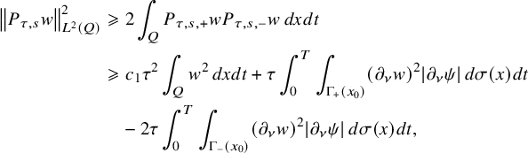 $$ \begin{align*} \left\lVert P_{\tau,s}w\right\rVert_{L^2(Q)}^2 &\geqslant2\int_QP_{\tau,s,+}wP_{\tau,s,-}w\, dxdt \\ &\geqslant c_1\tau^2\int_Qw^2\, dxdt+\tau\int_0^T\int_{\Gamma_{+}(x_0)} (\partial_\nu w)^2|\partial_\nu\psi| \, d\sigma(x)dt \\ &\quad -2\tau\int_0^T\int_{\Gamma_{-}(x_0)} (\partial_\nu w)^2|\partial_\nu\psi| \, d\sigma(x)dt, \end{align*} $$
with $c_1>0$
depending only on
$c_1>0$
depending only on $\Omega $
. From this last estimate and the fact that
$\Omega $
. From this last estimate and the fact that
 $$ \begin{align*} \partial_\nu\psi(x)=\frac{(x-x_0)\cdot\nu}{|x-x_0|},\quad x\in\partial\Omega, \end{align*} $$
we deduce easily (A.2).
Acknowledgments
T.L. was supported by the Academy of Finland (Centre of Excellence in Inverse Modeling and Imaging, grant numbers 284715 and 309963). Y.-H.L. is partially supported by the National Science and Technology Council (NSTC) Taiwan, under the projects 111-2628-M-A49-002 and 112-2628-M-A49-003. Y.-H.L. is also a Humboldt research fellow.
Competing interest
The authors have no competing interest to declare.

 Open access