


1. Introduction
Over the past decade, market-consistent actuarial valuation techniques for quantifying risk have been increasingly embraced not only by academic research but also by the insurance industry, a development that has consequently led to the measurement of assets and liabilities. This shift has been driven by both regulatory and accounting standards and is reflected in frameworks such as the Solvency II Directive (European Parliament and Council, 2021) and the International Financial Reporting Standards (IFRS Foundation, 2017). In particular, under Solvency II, the valuation principle relies on fair value: assets and liabilities must be measured at amounts that could be exchanged or settled in an open market. The detailed valuation framework laid out in the Solvency II Delegated Acts (European Parliament and Council, 2014) prioritizes observable market prices where available. When the liabilities are not hedgeable, technical provisions are computed as the sum of the best estimate (BE) – the present value of expected future cashflows – and the risk margin (RM), which reflects the cost of capital associated with non-hedgeable risks (see, e.g., Olivieri & Pitacco, Reference Olivieri and Pitacco2008).
A key element of modern life-insurance valuation is the careful consideration of demographic risk (see, e.g., Asmussen & Steffensen, Reference Asmussen and Steffensen2020; Wüthrich & Merz, Reference Wüthrich and Merz2013), which captures the uncertainty related to mortality and longevity outcomes. These population-based uncertainties significantly impact the timing and amount of future benefit payments, making them crucial for both the valuation of insurance liabilities and the assessment of capital requirements. In this context, Savelli and Clemente (Reference Savelli and Clemente2013) develop a discrete-time model aimed at evaluating the capital requirement for a cohort of policyholders with homogeneous risks holding traditional life insurance policies, i.e., policies in which the sum insured is deterministic and not linked to financial variables, within a local Generally Accepted Accounting Principles (GAAP) framework. Subsequent studies, see Clemente et al. (Reference Clemente, Della Corte and Savelli2021) and (Reference Clemente, Della Corte and Savelli2022), focus on bridging the local GAAP framework with the market-consistent approach adopted under Solvency II. Within this framework, Wüthrich et al. (Reference Wüthrich, Bühlmann and Furrer2010) propose a model based on the concept of the Claims Development Result (CDR) – the random variable representing profits and losses over a one-year time horizon – used to quantify the risk associated with a cohort of policyholders holding the same type of policy.
In recent decades, insurance products have progressively shifted away from offering a fixed sum insured. Instead, the benefit amount is now tied to the performance of various financial variables, such as asset values, portfolios, or indices, giving rise to the concept of equity-linked policies. These contracts typically include embedded guarantees, which may take the form of terminal-value guarantees (i.e., guarantees at maturity) or Cliquet-type guarantees, where the policyholder annually compounds an interest equal to the maximum between a stochastic rate and a guaranteed minimum rate. A guarantee ensuring a minimum year-on-year return is particularly appealing to risk-averse policyholders, especially in environments characterized by severe, sporadic market downturns. Disruptive events such as the 2000 Dot-com bubble, the 2008 global financial crisis, the 2020 COVID-19 pandemic, the 2022 Russian invasion of Ukraine, and the ongoing 2025 uncertainty surrounding tariffs in the US have underscored the value of products that offer protection against severe market volatility while preserving some participation in upside gains during normal years.
In early contributions, Brennan and Schwartz (Reference Brennan and Schwartz1976) and (Reference Brennan and Schwartz1979) propose an actuarial model for pricing products with a minimum guarantee under no-arbitrage assumptions, leveraging the concept of a hedging portfolio. Specifically, abstracting from demographic considerations, they decompose the policy payoff into the payoffs of equities, bonds, and options. Subsequently, Bacinello (Reference Bacinello2001) introduces a no-arbitrage pricing approach for policies featuring Cliquet-style guarantees. More recently, Barigou and Delong (Reference Barigou and Delong2022) price equity-linked contracts under the assumption that the insurer hedges risks to minimize the local variance of the net asset value process, while requiring compensation for the non-hedgeable portion of the liability in the form of an instantaneous standard deviation RM.
The valuation of insurance products with financial components is therefore a well-established topic in the literature. Perman and Zalokar (Reference Perman and Zalokar2018) examine the conditions under which it becomes optimal to hedge liabilities using derivative instruments within the Cox-Ross-Rubinstein framework, while Møller (Reference Møller1998) focuses on the development of risk-minimizing trading strategies and analyzes the corresponding intrinsic risk processes for various types of unit-linked contracts.
With reference to demographic risk, much of the research has focused on quantifying longevity risk in isolation (see Yang & Zhou, 2023; Gasimova et al., Reference Gasimova, Haberman and Millossovich2025). For example, Stevens et al. (Reference Stevens, De Waegenaere and Melenberg2010) discuss how to determine capital reserves for longevity risk in life insurance under Solvency II, while Boonen (Reference Boonen2017) considers how the results under Solvency II would be affected by the choice of a different risk measure, i.e., Expected Shortfall rather than Value-at-Risk (VaR). Hari et al. (Reference Hari, De Waegenaere, Melenberg and Nijman2008) assess the impact of longevity risk on pension fund solvency, distinguishing between individual (micro) and population-wide (macro) mortality risks.
The fair dynamic valuation of insurance liabilities has been further explored by ensuring market- and time-consistency through mean-variance hedging in a multi-period setting (see Barigou & Dhaene, Reference Barigou and Dhaene2019), by merging actuarial judgment and market-consistency (see Dhaene et al., Reference Dhaene, Stassen, Barigou, Linders and Chen2017), and via a two-step generalized regression approach (see Barigou et al., 2021). Further research includes credit and interest rate risk (see, e.g., Bernard et al., Reference Bernard, Le Courtois and Quittard-Pinon2005; Grosen & Løchte Jørgensen, Reference Grosen and Løchte Jørgensen2000; Möhr, Reference Möhr2011). Comprehensive formulations for market-consistent liability valuations are offered in Wüthrich et al. (Reference Wüthrich, Bühlmann and Furrer2010) and Wüthrich and Merz (Reference Wüthrich and Merz2013), with recent developments introducing two- and three-step valuation procedures that integrate hedging techniques and risk measures (Linders, Reference Linders2023).
Recent work also includes Agarwal et al. (Reference Agarwal, Ewald and Wang2023), who solve a market-based optimal investment problem for a defined-contribution pension scheme with a minimum annuity-purchase guarantee via dynamic programming. They highlight the role of longevity bonds, explicitly distinguishing between systematic (non-diversifiable) and idiosyncratic (diversifiable) mortality risk. Similarly, Agarwal et al. (Reference Agarwal, Ewald and Wang2025), derive (semi-)analytic solutions to the Hamilton–Jacobi–Bellman for optimal investment and income drawdown under stochastic mortality with imperfectly correlated reference populations, showing that longevity bonds remain an effective hedge even in the presence of basis risk and when allowing for dependence between mortality and equity returns. These conceptual links closely relate to our decomposition of demographic uncertainty into idiosyncratic and trend components. In both frameworks, the non-diversifiable longevity component gives rise to market incompleteness, whereas the diversifiable component can be pooled or hedged. Our contribution offers an analogous decomposition and a dynamic market-consistent valuation in the context of equity-linked life insurance with Cliquet guarantees.
The existing literature provides limited insight into the integration of demographic risk modeling with market-consistent valuation, particularly in the context of capital requirement assessments. Bridging this gap would enable insurers to better understand their exposure to demographic risks – such as mortality and longevity – thus supporting more effective pricing, reserving, and capital management strategies. To this end, we propose a novel methodology for quantifying capital requirements related to demographic risk in an equity-linked insurance portfolio with a Cliquet-style guarantee. Building on the theoretical foundations in Wüthrich et al. (Reference Wüthrich, Bühlmann and Furrer2010), Wüthrich and Merz (Reference Wüthrich and Merz2013), our framework focuses on homogeneous risk groups and accounts for both idiosyncratic and trend risks, while also factoring in financial impacts through a market-consistent claims development approach.
Building on Clemente et al. (Reference Clemente, Della Corte, Savelli and Zappa2025), we present the model by moving beyond a purely matrix-based formulation and by providing a more explicit theoretical foundation for valuation and risk-capital analysis. Unlike Clemente et al. (Reference Clemente, Della Corte, Savelli and Zappa2025), who consider a terminal-value guarantee and yield results in line with traditional actuarial expectations, our work shifts the focus to year-on-year guarantees. To this end, we extend the VaPo and CDR framework with three main objectives. First, we establish a solid theoretical basis for the framework that underpins market-consistent valuation and risk measurement. Second, we complete the spectrum of guarantee designs by formally embedding year-on-year local guarantees within a unified market-consistent framework. In particular, the proposed structure generalizes the classical annual high step-up (ratchet) mechanism – typically corresponding to the case of a zero guaranteed rate – by allowing for a strictly positive annual guaranteed return. As a consequence, the guarantee base evolves according to a multiplicative local maximum rule that encompasses traditional reset and ratchet designs as special cases. This formulation makes the financial component of the liability amenable to dynamic hedging arguments consistent with modern arbitrage-free valuation theory. Third, we show that, under a Cliquet-type guarantee, the contract can exhibit negative sums-at-risk, thereby reversing the insurer’s demographic exposure, from mortality risk to longevity risk and vice versa, depending on the realized path of returns and guaranteed minimum rates.
Idiosyncratic risk, in our setting, consists of both diversifiable and systematic components: the former relates to random fluctuations and portfolio characteristics, while the latter reflects estimation uncertainty in mortality forecasting models. Throughout the paper, we use the term trend risk in the specific context of one-year updating as defined in Solvency II: it refers to the risk that the best-estimate mortality assumptions, and consequently the projected future death probabilities, are revised after observing one year of actual experience and recalibrating the selected stochastic mortality model. This definition is more specific than the broader notion of systematic longevity risk often adopted in the literature. In our framework, trend risk is precisely the component that drives the one-year revision of the BE and underlies the trend component of the change in future discretionary benefits.
We develop a comprehensive simulation-based framework that captures both sources of demographic risk and considers contract-specific features, such as a Cliquet guarantee and the dispersion of the sums insured across policyholders. A numerical case study illustrates the application of the model and highlights how the capital requirement is influenced by key factors, such as policyholder age, contract duration, volatility of the financial asset, and guaranteed rate. Death probabilities are projected using well-established stochastic mortality models, including Lee-Carter (LC) (Brouhns et al., Reference Brouhns, Denuit and Vermunt2002), Cairns–Blake–Dowd (Reference Cairns, Blake and Dowd2006), and Renshaw–Haberman (Reference Renshaw and Haberman2006), with model uncertainty incorporated into the Solvency Capital Requirement (SCR) estimation.
While designed within the Solvency II regulatory context, the proposed framework is adaptable to alternative regimes and can serve as both a regulatory tool and an internal risk management tool. Furthermore, although our focus is on equity-linked contracts, the methodology naturally extends to traditional insurance products featuring constant benefits.
The remainder of the paper is organized as follows. Section 2 introduces the financial market and the cohort of policyholders. Section 3 outlines the valuation framework for evaluating cash inflows and outflows related to the contract, along with the strategy to replicate and price the contingent claim. In Section 4, we focus on demographic risk, examining its idiosyncratic and trend components, and propose a methodology to assess the capital requirements associated with each component. A numerical analysis is presented in Section 5. Section 6 concludes.
2. Financial and insurance environment
Consider a complete probability space
 $\left (\Omega , \mathcal{F}, \mathbb{P}\right )$
equipped with a complete and right–continuous filtration
$\left (\Omega , \mathcal{F}, \mathbb{P}\right )$
equipped with a complete and right–continuous filtration
 $\mathbb{F}=\left (\mathcal{F}_t\right )_{t\in [0,n]}$
satisfying the usual conditions. The time horizon
$\mathbb{F}=\left (\mathcal{F}_t\right )_{t\in [0,n]}$
satisfying the usual conditions. The time horizon
 $n\lt +\infty$
is expressed in years.
$n\lt +\infty$
is expressed in years.
In the probability space
 $(\Omega ,\mathcal F,\mathbb P)$
, we define a Wiener process
$(\Omega ,\mathcal F,\mathbb P)$
, we define a Wiener process
 $W=(W_t)_{t\in [0,n]}$
modeling financial risk. We denote by
$W=(W_t)_{t\in [0,n]}$
modeling financial risk. We denote by
 $\mathbb F^W=(\mathcal F_t^W)_{t\in [0,n]}$
the subfiltration generated by
$\mathbb F^W=(\mathcal F_t^W)_{t\in [0,n]}$
the subfiltration generated by
 $W$
, where
$W$
, where
 $ \mathcal F_t^W \;:\!=\; \sigma \left (W_u:\,0\le u\le t\right )$
,
$ \mathcal F_t^W \;:\!=\; \sigma \left (W_u:\,0\le u\le t\right )$
,
 $t\in [0,n]$
. The subfiltration
$t\in [0,n]$
. The subfiltration
 $\mathbb F^W$
represents the information generated by financial market variables.
$\mathbb F^W$
represents the information generated by financial market variables.
Insurance risk is described by an additional source of uncertainty whose detailed structure will be specified in Subsection 2.2. Since insurance events are observed at yearly dates, we model the corresponding information flow through a subfiltration
 $(\mathcal{F}_t^{\mathbb I})_{t\in [0,n]}$
that evolves only on the annual grid and remains constant between observation dates.
$(\mathcal{F}_t^{\mathbb I})_{t\in [0,n]}$
that evolves only on the annual grid and remains constant between observation dates.
Assumption 2.1.
The subfiltrations
 $\mathbb{F}^W =(\mathcal{F}_t^W)_{t\in [0,n]}$
and
$\mathbb{F}^W =(\mathcal{F}_t^W)_{t\in [0,n]}$
and
 $\mathbb{F}^{\mathbb{I}} =(\mathcal{F}_t^{\mathbb{I}})_{t\in [0,n]}$
are independent (under
$\mathbb{F}^{\mathbb{I}} =(\mathcal{F}_t^{\mathbb{I}})_{t\in [0,n]}$
are independent (under
 $\mathbb{P}$
), and we set
$\mathbb{P}$
), and we set
 $\mathcal{F}_t \;:\!=\; \mathcal{F}_t^W \vee \mathcal{F}_t^{\mathbb{I}}$
 $(t=0,\ldots ,n)$
.
$(t=0,\ldots ,n)$
.
Under Assumption 2.1, financial and insurance risks are independent. This assumption, which is standard in the actuarial literature (see Wüthrich et al., Reference Wüthrich, Bühlmann and Furrer2010), is introduced for analytical tractability and to clearly disentangle demographic (insurance) risk from financial market dynamics in the subsequent valuation and hedging analysis. We proceed by introducing the financial market and the cohort of policyholders.
2.1 The financial market
We consider a risky asset
 $\mathcal{S}$
whose time-
$\mathcal{S}$
whose time-
 $t$
price,
$t$
price,
 $S_t$
, is described under the objective probability measure
$S_t$
, is described under the objective probability measure
 $\mathbb{P}$
by the following dynamics:
$\mathbb{P}$
by the following dynamics:
 \begin{equation} \mathrm{d}S_t=\mu _t S_t \mathrm{d}t + \sigma _t S_t \mathrm{d}W_t. \end{equation}
The stochastic differential equation above suggests that the price of the risky asset follows a geometric Brownian motion, where the time-varying parameters are the drift
 $\mu _t$
and the relative volatility
$\mu _t$
and the relative volatility
 $\sigma _t$
.
$\sigma _t$
.
We then characterize the bond market and assume deterministic dynamics of the term structure of interest rates, implying that the time-
 $t$
instantaneous forward rate for a future date
$t$
instantaneous forward rate for a future date
 $\tau \gt t$
,
$\tau \gt t$
,
 $f_{t,\tau }$
, coincides with the actual time-
$f_{t,\tau }$
, coincides with the actual time-
 $\tau$
instantaneous interest rate,
$\tau$
instantaneous interest rate,
 $r_\tau$
. Consequently, denoting with
$r_\tau$
. Consequently, denoting with
 $B\left (t,\tau \right )$
the time-
$B\left (t,\tau \right )$
the time-
 $t$
price of a default-free zero-coupon bond maturing at time
$t$
price of a default-free zero-coupon bond maturing at time
 $\tau \gt t$
, the following relation holds:
$\tau \gt t$
, the following relation holds:
 \begin{equation} r_\tau = f_{t,\tau } = -\dfrac { \partial \ln \left (B \left ( t,\tau \right ) \right ) } {\partial \tau }. \end{equation}
Different zero-coupon bonds
 $\mathcal{B}_i$
(
$\mathcal{B}_i$
(
 $i\in \left \{1,\ldots ,N_{\mathcal{B}}\right \}$
) are traded on the financial market, with maturities given by
$i\in \left \{1,\ldots ,N_{\mathcal{B}}\right \}$
) are traded on the financial market, with maturities given by
 $T_{\mathcal{B}_i}$
and time-
$T_{\mathcal{B}_i}$
and time-
 $t$
prices denoted by
$t$
prices denoted by
 $B_{i,t}=B(t,T_{\mathcal{B}_i} )$
.
$B_{i,t}=B(t,T_{\mathcal{B}_i} )$
.
Finally, we assume that European put options
 $\mathcal{P}_i$
(
$\mathcal{P}_i$
(
 $i\in \left \{1,\ldots ,N_{\mathcal{P}}\right \}$
) written on the underlying risky asset
$i\in \left \{1,\ldots ,N_{\mathcal{P}}\right \}$
) written on the underlying risky asset
 $\mathcal{S}$
are traded on the market. The strike prices and maturities of the put options are
$\mathcal{S}$
are traded on the market. The strike prices and maturities of the put options are
 $K_{\mathcal{P}_i}$
and
$K_{\mathcal{P}_i}$
and
 $T_{\mathcal{P}_i}$
, respectively, while the time-
$T_{\mathcal{P}_i}$
, respectively, while the time-
 $t$
prices of the options are denoted by
$t$
prices of the options are denoted by
 $P_{i,t}=P(t,T_{\mathcal{P}_i},K_{\mathcal{P}_i})$
.
$P_{i,t}=P(t,T_{\mathcal{P}_i},K_{\mathcal{P}_i})$
.
In the following section, we derive a strategy replicating the financial claim and provide additional details on the maturities of the bonds, as well as on the maturities and strike prices of the put options, that are needed to construct the replicating strategy. The time-
 $t$
trading strategy (
$t$
trading strategy (
 $t\in \left \{0,\ldots ,n-1\right \}$
) is defined as a multi-dimensional process
$t\in \left \{0,\ldots ,n-1\right \}$
) is defined as a multi-dimensional process
 $\left \{\boldsymbol{\theta }_t\right \}_{t\in \left \{0,\ldots ,n-1\right \}}$
predictable with respect to the filtration
$\left \{\boldsymbol{\theta }_t\right \}_{t\in \left \{0,\ldots ,n-1\right \}}$
predictable with respect to the filtration
 $\mathbb{F}^W$
, i.e.,
$\mathbb{F}^W$
, i.e.,
 $\boldsymbol{\theta }_t$
is
$\boldsymbol{\theta }_t$
is
 $\mathcal{F}_{t}^W$
-measurable. More precisely,
$\mathcal{F}_{t}^W$
-measurable. More precisely,
 $\boldsymbol{\theta }_t=\left (\theta ^{\mathcal{S}}_t,\theta ^{\mathcal{B}_1}_t,\ldots ,\theta ^{\mathcal{B}_{N_{\mathcal{B}}}}_t,\theta ^{\mathcal{P}_1}_t,\ldots ,\theta ^{\mathcal{P}_{N_{\mathcal{P}}}}_t\right )$
, where
$\boldsymbol{\theta }_t=\left (\theta ^{\mathcal{S}}_t,\theta ^{\mathcal{B}_1}_t,\ldots ,\theta ^{\mathcal{B}_{N_{\mathcal{B}}}}_t,\theta ^{\mathcal{P}_1}_t,\ldots ,\theta ^{\mathcal{P}_{N_{\mathcal{P}}}}_t\right )$
, where
 $\theta ^{\mathcal{S}}_t$
is the number of units invested in the stock
$\theta ^{\mathcal{S}}_t$
is the number of units invested in the stock
 $\mathcal{S}$
at time
$\mathcal{S}$
at time
 $t$
, i.e., for the time interval
$t$
, i.e., for the time interval
 $\left (t,t+1\right ]$
, while
$\left (t,t+1\right ]$
, while
 $\theta ^{\mathcal{B}_i}_t$
and
$\theta ^{\mathcal{B}_i}_t$
and
 $\theta ^{\mathcal{P}_i}_t$
are the analogous for bonds and put options.
$\theta ^{\mathcal{P}_i}_t$
are the analogous for bonds and put options.
Assumption 2.2. We assume that the financial market of traded assets is arbitrage-free and complete.
We consider a continuous-time financial market on the time horizon
 $[0,n]$
and work under the objective probability measure
$[0,n]$
and work under the objective probability measure
 $\mathbb{P}$
, where the source of uncertainty is the Brownian motion
$\mathbb{P}$
, where the source of uncertainty is the Brownian motion
 $W$
. Let
$W$
. Let
 $\lambda =\left (\lambda _t\right )_{t\in [0,n]}$
be an
$\lambda =\left (\lambda _t\right )_{t\in [0,n]}$
be an
 $\mathbb{F}^W$
-adapted market price of risk process.Footnote 1 Define the stochastic discount factor (density process)
$\mathbb{F}^W$
-adapted market price of risk process.Footnote 1 Define the stochastic discount factor (density process)
 $\xi ^\lambda =\left (\xi _t^\lambda \right )_{t\in [0,n]}$
by
$\xi ^\lambda =\left (\xi _t^\lambda \right )_{t\in [0,n]}$
by
 \begin{equation} \xi _t^\lambda =\exp \left \{-\int _{0}^{t}\lambda _s\, \mathrm{d}W_s-\frac {1}{2}\int _{0}^{t}\lambda _s^{2}\, \mathrm{d}s\right \}. \end{equation}
Under the above integrability conditions,
 $\xi ^\lambda$
is a strictly positive
$\xi ^\lambda$
is a strictly positive
 $\mathbb{P}$
-martingale. Hence, following Munk (Reference Munk2013), we define an equivalent probability measure
$\mathbb{P}$
-martingale. Hence, following Munk (Reference Munk2013), we define an equivalent probability measure
 $\mathbb{Q}$
on
$\mathbb{Q}$
on
 $(\Omega ,\mathcal{F}_n)$
via the Radon–Nikodym derivative
$(\Omega ,\mathcal{F}_n)$
via the Radon–Nikodym derivative
 $\frac {\mathrm{d}\mathbb{Q}}{\mathrm{d}\mathbb{P}}\Big |_{\mathcal{F}_n} \;:\!=\; \xi _n^\lambda ,$
so that
$\frac {\mathrm{d}\mathbb{Q}}{\mathrm{d}\mathbb{P}}\Big |_{\mathcal{F}_n} \;:\!=\; \xi _n^\lambda ,$
so that
 $\xi _t^\lambda =\mathbb{E}^{\mathbb{P}}\left [\left .\frac {\mathrm{d}\mathbb{Q}}{\mathrm{d}\mathbb{P}}\right |\mathcal{F}_t^W\right ]$
for all
$\xi _t^\lambda =\mathbb{E}^{\mathbb{P}}\left [\left .\frac {\mathrm{d}\mathbb{Q}}{\mathrm{d}\mathbb{P}}\right |\mathcal{F}_t^W\right ]$
for all
 $t\in [0,n]$
.
$t\in [0,n]$
.
In our framework, the absence of arbitrage and the completeness of the market are equivalent to the existence of a unique equivalent martingale measure
 $\mathbb{Q}$
. Under
$\mathbb{Q}$
. Under
 $\mathbb{Q}$
, the discounted price processes are
$\mathbb{Q}$
, the discounted price processes are
 $\mathbb{F}^W$
-martingales and, in particular, for
$\mathbb{F}^W$
-martingales and, in particular, for
 $t\in \{1,\ldots ,n\}$
,
$t\in \{1,\ldots ,n\}$
,
 \begin{align} & S_{t-1} = \mathbb{E}^{\mathbb{Q}}_{t-1} \left [e^{-\int _{t-1}^{t}r_s\,\mathrm{d}s}\,S_t \right ], \end{align}
 \begin{align} & B_{i,t-1} = \mathbb{E}^{\mathbb{Q}}_{t-1} \left [e^{-\int _{t-1}^{t}r_s\,\mathrm{d}s}\,B_{i,t} \right ] \quad \forall i\in \left \{1,\ldots ,N_{\mathcal{B}}\right \}, \end{align}
 \begin{align} & P_{i,t-1} = \mathbb{E}^{\mathbb{Q}}_{t-1} \left [e^{-\int _{t-1}^{t}r_s\,\mathrm{d}s}\,P_{i,t} \right ] \quad \forall i\in \left \{1,\ldots ,N_{\mathcal{P}}\right \}. \end{align}
Note that we use the notation
 $\mathbb{E}^{\mathbb{Q}}_t\left [\cdot \right ]=\mathbb{E}^{\mathbb{Q}}\big[\cdot \big |\mathcal{F}_{t}^W\big ]$
. For a proof of this equivalence, we refer to Delbaen and Schachermayer (Reference Delbaen and Schachermayer2006).
$\mathbb{E}^{\mathbb{Q}}_t\left [\cdot \right ]=\mathbb{E}^{\mathbb{Q}}\big[\cdot \big |\mathcal{F}_{t}^W\big ]$
. For a proof of this equivalence, we refer to Delbaen and Schachermayer (Reference Delbaen and Schachermayer2006).
2.2 The cohort of policyholders
We assume that, at time
 $t=0$
, a cohort of
$t=0$
, a cohort of
 $\ell _0\in \mathbb{N}_{\neq 0}$
policyholders with identical characteristics (same entry age
$\ell _0\in \mathbb{N}_{\neq 0}$
policyholders with identical characteristics (same entry age
 $x$
, policy term, premium payment pattern, etc.) enters the insurer’s portfolio. The insurer sells equity-linked endowment policies with a Cliquet guarantee to this cohort. Hence, risks are homogeneous across policyholders, except for the sum insured: each policyholder
$x$
, policy term, premium payment pattern, etc.) enters the insurer’s portfolio. The insurer sells equity-linked endowment policies with a Cliquet guarantee to this cohort. Hence, risks are homogeneous across policyholders, except for the sum insured: each policyholder
 $k\in \{1,\ldots ,\ell _0\}$
subscribes to the same contract structure with an individual sum insured
$k\in \{1,\ldots ,\ell _0\}$
subscribes to the same contract structure with an individual sum insured
 $c_{k,0}$
. We assume that lapses (surrenders) are not allowed over the contract term, so that the only cause of contract termination before maturity is death.
$c_{k,0}$
. We assume that lapses (surrenders) are not allowed over the contract term, so that the only cause of contract termination before maturity is death.
Let
 $T_{k,x}$
denote the (unconditional) future lifetime in years of policyholder
$T_{k,x}$
denote the (unconditional) future lifetime in years of policyholder
 $k$
measured from time
$k$
measured from time
 $t=0$
. Working in discrete time (annual periods), we define the residual lifetime at time
$t=0$
. Working in discrete time (annual periods), we define the residual lifetime at time
 $t$
by the convention
$t$
by the convention
 \begin{equation} T_{k,x+t} \;:\!=\; \max [T_{k,x}-t,0], \quad t=0,1,\ldots , \quad k\in \{1,\ldots ,\ell _0\}. \end{equation}
In particular,
 $T_{k,x+t}=0$
when death occurs at or before time
$T_{k,x+t}=0$
when death occurs at or before time
 $t$
. If
$t$
. If
 $\{T_{k,x}\gt t\}$
, death occurs after time
$\{T_{k,x}\gt t\}$
, death occurs after time
 $t$
and
$t$
and
 $T_{k,x+t}=T_{k,x}-t$
represents the remaining lifetime measured from time
$T_{k,x+t}=T_{k,x}-t$
represents the remaining lifetime measured from time
 $t$
.
$t$
.
Consistent with the benefit structure of an endowment contract, we introduce the following indicator:
 \begin{equation} \mathbb{I}_{k,t}\;:\!=\; \begin{cases} \unicode {x1D7D9}_{\{T_{k,x+t}\in (0,1]\}}, & t=0,\ldots ,n-2,\\ \unicode {x1D7D9}_{\{T_{k,x+t}\gt 0\}}, & t=n-1. \end{cases} \qquad k\in \{1,\ldots ,\ell _0\}. \end{equation}
For
 $t=0,\ldots ,n-2$
, the event
$t=0,\ldots ,n-2$
, the event
 $\{\mathbb{I}_{k,t}=1\}$
means that policyholder
$\{\mathbb{I}_{k,t}=1\}$
means that policyholder
 $k$
dies during the period
$k$
dies during the period
 $(t,t+1]$
, thereby representing the occurrence of the insured event that triggers a death benefit payment at time
$(t,t+1]$
, thereby representing the occurrence of the insured event that triggers a death benefit payment at time
 $t+1$
. Accordingly, the sequence
$t+1$
. Accordingly, the sequence
 $\{\mathbb{I}_{k,t}\}_{t=0}^{n-2}$
describes whether the policy is in force up to each time
$\{\mathbb{I}_{k,t}\}_{t=0}^{n-2}$
describes whether the policy is in force up to each time
 $t$
. The final line in (2.8) is a contractual convention: at maturity (time
$t$
. The final line in (2.8) is a contractual convention: at maturity (time
 $n$
), the endowment benefit is payable only if the contract is still in force at time
$n$
), the endowment benefit is payable only if the contract is still in force at time
 $n-1$
, which is equivalent to
$n-1$
, which is equivalent to
 $\{T_{k,x+t}\gt 0\}$
. This convention allows the use of a single indicator process
$\{T_{k,x+t}\gt 0\}$
. This convention allows the use of a single indicator process
 $\{\mathbb{I}_{k,t}\}_{t=0}^{n-1}$
to model both the in-force status over time and the endowment payoff at maturity.
$\{\mathbb{I}_{k,t}\}_{t=0}^{n-1}$
to model both the in-force status over time and the endowment payoff at maturity.
For each
 $t=0,\ldots ,n-2$
, the indicator
$t=0,\ldots ,n-2$
, the indicator
 $\mathbb{I}_{k,t}$
is observed at time
$\mathbb{I}_{k,t}$
is observed at time
 $t+1$
and is therefore
$t+1$
and is therefore
 $\mathcal{F}_{t+1}^{\mathbb{I}}$
-measurable (and hence also
$\mathcal{F}_{t+1}^{\mathbb{I}}$
-measurable (and hence also
 $\mathcal{F}_{t+1}$
-measurable). Moreover, under Assumption 2.1,
$\mathcal{F}_{t+1}$
-measurable). Moreover, under Assumption 2.1,
 $\mathbb{I}_{k,t}$
is independent of
$\mathbb{I}_{k,t}$
is independent of
 $\mathcal{F}_t^W$
.
$\mathcal{F}_t^W$
.
Assumption 2.3 (Conditional i.i.d. mortality (among survivors)). For each
 $t=0,\ldots ,n-2$
, let
$t=0,\ldots ,n-2$
, let
 $Q_{x+t}$
denote the stochastic one-year death probability at age
$Q_{x+t}$
denote the stochastic one-year death probability at age
 $x+t$
in the standard actuarial sense, i.e., conditional on being alive at time
$x+t$
in the standard actuarial sense, i.e., conditional on being alive at time
 $t$
.
$t$
.
Define the (random) set of policyholders alive at time
 $t$
by
$t$
by
 \begin{equation} \mathcal L_t \;:\!=\; \{k\in \{1,\ldots ,\ell _0\}:\ T_{k,x}\gt t\}, \qquad \ell _t \;:\!=\; |\mathcal L_t|, \end{equation}
where
 $\ell _t$
is the number of policyholders alive at time
$\ell _t$
is the number of policyholders alive at time
 $t$
.
$t$
.
Conditional on
 $Q_{x+t}$
, the random variables
$Q_{x+t}$
, the random variables
 $\{\mathbb I_{k,t}\}_{k\in \mathcal L_t}$
are independent and identically distributed. Hence,
$\{\mathbb I_{k,t}\}_{k\in \mathcal L_t}$
are independent and identically distributed. Hence,
 \begin{equation} \mathbb{I}_{k,t}\,\big |\,\left (Q_{x+t},\,k\in \mathcal L_t\right )\sim \mathrm{Ber}(Q_{x+t}). \end{equation}
Moreover, for any distinct
 $h,k$
,
$h,k$
,
 \begin{equation} \mathbb{P}(\mathbb{I}_{h,t}=1,\mathbb{I}_{k,t}=1\,|\,Q_{x+t},\,h\in \mathcal L_t,\,k\in \mathcal L_t) = Q_{x+t}^{2}. \end{equation}
Finally, we define the best-estimate (one-year) death probability at time
 $t$
as
$t$
as
 \begin{equation} q_{x+t}\;:\!=\; \mathbb{E}^{\mathbb{P}}\left [Q_{x+t}\,\big |\,\mathcal F_t\right ], \end{equation}
i.e., the conditional expectation given the information available up to time
 $t$
.
$t$
.
At a generic time
 $t\in \{1,\ldots ,n-1\}$
, the sum insured in force for policyholder
$t\in \{1,\ldots ,n-1\}$
, the sum insured in force for policyholder
 $k$
is given by
$k$
is given by
 \begin{equation} C_{k,t}\;:\!=\; c_{k,0}\prod _{s=0}^{t-1}\left (1-\mathbb{I}_{k,s}\right ), \qquad k\in \{1,\ldots ,\ell _0\}, \end{equation}
which equals
 $c_{k,0}$
if no death has occurred up to time
$c_{k,0}$
if no death has occurred up to time
 $t$
and
$t$
and
 $0$
otherwise. This representation is convenient at the portfolio level, as it allows for modeling the in-force status of contracts and to aggregate mortality-driven cash flows across policyholders.
$0$
otherwise. This representation is convenient at the portfolio level, as it allows for modeling the in-force status of contracts and to aggregate mortality-driven cash flows across policyholders.
3. Cashflows, pricing, and reserving
3.1 Premiums and benefits
Assumption 3.1.
Considering a generic time span
 $\left (t,t+1\right ]$
, the premiums are paid by the policyholders at the beginning of the period, i.e., in
$\left (t,t+1\right ]$
, the premiums are paid by the policyholders at the beginning of the period, i.e., in
 $t^+$
, while the sums insured of occurred deaths/survivals are paid at the end of the year (i.e., in
$t^+$
, while the sums insured of occurred deaths/survivals are paid at the end of the year (i.e., in
 $t+1$
).
$t+1$
).
We first define the
 $\mathbb{F}$
-adapted vector of the cashflows, generically indicated with
$\mathbb{F}$
-adapted vector of the cashflows, generically indicated with
 $\textbf {X}$
:
$\textbf {X}$
:
 \begin{equation} \textbf {X}_{(0)}=(\textit {X}_0,\textit {X}_1,\ldots ,\textit {X}_n). \end{equation}
Considering two vectors of random variables,
 $\textbf {X}$
and
$\textbf {X}$
and
 $\textbf {Y}$
, both of dimension
$\textbf {Y}$
, both of dimension
 $n\times 1$
, we assume
$n\times 1$
, we assume
 \begin{align} \mathbb{E}\left [\sum _{t=0}^{n}X^2_t\right ]&\lt \infty , \end{align}
 \begin{align} \mathbb{E}\left [\sum _{t=0}^{n}X_t\cdot Y_t\right ]&\lt \infty . \end{align}
Consequently,
 $\textbf {X}\in L^2_{n+1}\left (\mathbb{P},\mathbb{F}\right )$
, where
$\textbf {X}\in L^2_{n+1}\left (\mathbb{P},\mathbb{F}\right )$
, where
 $L^2_{n+1}\left (\mathbb{P},\mathbb{F}\right )$
is a
$L^2_{n+1}\left (\mathbb{P},\mathbb{F}\right )$
is a
 $(n+1)$
-dimensional Hilbert space. For a generic time
$(n+1)$
-dimensional Hilbert space. For a generic time
 $t$
, we define inflows and outflows, representing cashflows as follows:
$t$
, we define inflows and outflows, representing cashflows as follows:
 \begin{equation} X_\tau \;:\!=\; \begin{cases} -X_\tau ^{in} & \text{if $\tau =t$,} \\[5pt] X_\tau ^{out}-X_\tau ^{in} & \text{if $t\lt \tau \lt n$,}\\[5pt] X_\tau ^{out} & \text{if $\tau =n$}, \end{cases} \end{equation}
where
 \begin{align} X_\tau ^{in} & \;:\!=\; \sum _{k=1}^{\ell _0}C_{k,\tau }\cdot \pi \cdot U_{\tau ,\tau }^{in}, \end{align}
 \begin{align} X_\tau ^{out} & \;:\!=\;\sum _{k=1}^{\ell _0}C_{k,\tau -1}\cdot \mathbb{I}_{k,\tau -1}\cdot U_{\tau ,\tau }^{out}. \end{align}
In formula (3.4), the generic time-
 $\tau$
cashflow,
$\tau$
cashflow,
 $X_\tau$
, is given by the sum of two components: the inflow
$X_\tau$
, is given by the sum of two components: the inflow
 $X_\tau ^{in}$
and the outflow
$X_\tau ^{in}$
and the outflow
 $X_\tau ^{out}$
. According to Assumption 3.1, the former are paid at the beginning of each time period and the latter at the end.
$X_\tau ^{out}$
. According to Assumption 3.1, the former are paid at the beginning of each time period and the latter at the end.
The inflow received from the
 $k$
-th policyholder is the product of three terms: the sum insured at time
$k$
-th policyholder is the product of three terms: the sum insured at time
 $\tau$
,
$\tau$
,
 $C_{k,\tau }$
, the regular premium rate,
$C_{k,\tau }$
, the regular premium rate,
 $\pi$
, and the payout of a unit zero-coupon bond maturing at
$\pi$
, and the payout of a unit zero-coupon bond maturing at
 $\tau$
,
$\tau$
,
 $U_{\tau ,\tau }^{in}$
. Although the last factor is identically equal to one and could be formally omitted, its role will be clear when the hedging portfolio and the mathematical reserve are determined.
$U_{\tau ,\tau }^{in}$
. Although the last factor is identically equal to one and could be formally omitted, its role will be clear when the hedging portfolio and the mathematical reserve are determined.
Regarding the outflows, the benefit of the
 $k$
-th policyholder is the product of the sum insured at time
$k$
-th policyholder is the product of the sum insured at time
 $\tau -1$
,
$\tau -1$
,
 $C_{k,\tau -1}$
, a binary variable equal to
$C_{k,\tau -1}$
, a binary variable equal to
 $1$
if the beneficiary becomes eligible for the benefit at time
$1$
if the beneficiary becomes eligible for the benefit at time
 $t$
,
$t$
,
 $\mathbb{I}_{k,\tau -1}$
, and the (unitary) revaluation of the sum assured,
$\mathbb{I}_{k,\tau -1}$
, and the (unitary) revaluation of the sum assured,
 $U_{\tau ,\tau }^{out}$
. In accordance with the definition of a Cliquet guarantee (see Hipp, Reference Hipp1996; Bacinello, Reference Bacinello2001), such revaluation is defined as:
$U_{\tau ,\tau }^{out}$
. In accordance with the definition of a Cliquet guarantee (see Hipp, Reference Hipp1996; Bacinello, Reference Bacinello2001), such revaluation is defined as:
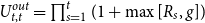
 \begin{equation} U_{\tau ,\tau }^{\textit {out}}\;:\!=\;\prod _{s=1}^{\tau } (1+\max [R_s,g] ), \end{equation}
where
 $R_s=\frac {S_s-S_{s-1}}{S_{s-1}}$
is the arithmetic return of the stock between time
$R_s=\frac {S_s-S_{s-1}}{S_{s-1}}$
is the arithmetic return of the stock between time
 $s-1$
and time
$s-1$
and time
 $s$
, while
$s$
, while
 $g$
is the guaranteed per-period return.
$g$
is the guaranteed per-period return.
The quantity
 $U^{out}_{\tau ,\tau }$
is the time-
$U^{out}_{\tau ,\tau }$
is the time-
 $\tau$
payoff factor per unit of sum insured generated by the Cliquet crediting rule. It represents the value at time
$\tau$
payoff factor per unit of sum insured generated by the Cliquet crediting rule. It represents the value at time
 $\tau$
of one monetary unit that is revalued each year by the credited gross return
$\tau$
of one monetary unit that is revalued each year by the credited gross return
 $1+\max [R_s,g]$
. Accordingly,
$1+\max [R_s,g]$
. Accordingly,
 $U^{out}_{\tau ,\tau }$
is an
$U^{out}_{\tau ,\tau }$
is an
 $\mathcal{F}^W_\tau$
-measurable random variable (i.e., a contingent claim), whereas
$\mathcal{F}^W_\tau$
-measurable random variable (i.e., a contingent claim), whereas
 $U^{out}_{t,\tau }$
denotes its time-
$U^{out}_{t,\tau }$
denotes its time-
 $t$
market-consistent value obtained via the replicating portfolio constructed below.
$t$
market-consistent value obtained via the replicating portfolio constructed below.
3.2 Replication and pricing of the contingent claim
Given
 $\tau \in [0,\ldots ,n]$
, the quantities
$\tau \in [0,\ldots ,n]$
, the quantities
 $\left (U_{t,\tau }^{in}\right )_{t=0,\ldots ,n}$
and
$\left (U_{t,\tau }^{in}\right )_{t=0,\ldots ,n}$
and
 $\left (U_{t,\tau }^{out}\right )_{t=0,\ldots ,n}$
are
$\left (U_{t,\tau }^{out}\right )_{t=0,\ldots ,n}$
are
 $\mathbb{F}^W$
-adapted stochastic processes representing the time-
$\mathbb{F}^W$
-adapted stochastic processes representing the time-
 $t$
values of the financial portfolios
$t$
values of the financial portfolios
 $\mathcal{U}^{in}_{t,\tau }$
and
$\mathcal{U}^{in}_{t,\tau }$
and
 $\mathcal{U}^{out}_{t,\tau }$
, respectively used at time
$\mathcal{U}^{out}_{t,\tau }$
, respectively used at time
 $t$
to replicate the time-
$t$
to replicate the time-
 $\tau$
quantities
$\tau$
quantities
 $U_{\tau ,\tau }^{in}$
and
$U_{\tau ,\tau }^{in}$
and
 $U_{\tau ,\tau }^{out}$
. While replicating the inflows is straightforward through zero-coupon bonds paying off future premiums, replicating the outflows is more challenging, due to the stochastic and nonlinear nature of the benefit in equation (3.7). The following theorem provides a replicating strategy and the price of the contingent claim.
$U_{\tau ,\tau }^{out}$
. While replicating the inflows is straightforward through zero-coupon bonds paying off future premiums, replicating the outflows is more challenging, due to the stochastic and nonlinear nature of the benefit in equation (3.7). The following theorem provides a replicating strategy and the price of the contingent claim.
Theorem 1.
The claim
 $U_{\tau ,\tau }^{\textit {out}}$
is
$U_{\tau ,\tau }^{\textit {out}}$
is
 $t$
-hedgeable because there exists a time-
$t$
-hedgeable because there exists a time-
 $t$
self-financing strategy
$t$
self-financing strategy
 $\boldsymbol{\theta }_{t,\tau }\in \Theta _{t,\tau }$
, with the following positions in the asset
$\boldsymbol{\theta }_{t,\tau }\in \Theta _{t,\tau }$
, with the following positions in the asset
 $\mathcal{S}$
and a European put option
$\mathcal{S}$
and a European put option
 $\mathcal{P}_t$
with a strike price
$\mathcal{P}_t$
with a strike price
 $S_t(1+g)$
expiring at time
$S_t(1+g)$
expiring at time
 $t+1$
:
$t+1$
:
 \begin{align} \theta _{t,\tau }^{\mathcal{S}} & =\frac {U_{t,\tau }^{\textit {out}}}{S_t+P_t}, \end{align}
 \begin{align} \theta _{t,\tau }^{\mathcal{P}_t} & =\frac {U_{t,\tau }^{\textit {out}}}{S_t+P_t}. \end{align}
 $U_{t,\tau }^{\textit {out}}$
is the time-
$U_{t,\tau }^{\textit {out}}$
is the time-
 $t$
price of the claim,
$t$
price of the claim,
 \begin{equation} U_{t,\tau }^{\textit {out}}=U_{t,t}^{\textit {out}}\prod _{h=t}^{\tau -1}(1+p_h), \end{equation}
where
 $P_t=S_t p_t$
is the no-arbitrage price of the put option
$P_t=S_t p_t$
is the no-arbitrage price of the put option
 $\mathcal{P}_t$
and
$\mathcal{P}_t$
and
 $p_{t}$
represents the Black-Scholes price of a European put option on an underlying asset with current price equal to one, strike price equal to
$p_{t}$
represents the Black-Scholes price of a European put option on an underlying asset with current price equal to one, strike price equal to
 $1+g$
, time-to-maturity equal to the time period
$1+g$
, time-to-maturity equal to the time period
 $\Delta t$
(equal to one under yearly frequency), interest rate
$\Delta t$
(equal to one under yearly frequency), interest rate
 $r_{t,t+1}=\frac {1}{\Delta t}\int _{t}^{t+1}r_{s}\mathrm{d}s$
, and volatility
$r_{t,t+1}=\frac {1}{\Delta t}\int _{t}^{t+1}r_{s}\mathrm{d}s$
, and volatility
 $\sigma _{t,t+1}=\sqrt {\frac {1}{\Delta t}\int _{t}^{t+1}\sigma _{s}^{2}\mathrm{d}s}$
:
$\sigma _{t,t+1}=\sqrt {\frac {1}{\Delta t}\int _{t}^{t+1}\sigma _{s}^{2}\mathrm{d}s}$
:
 \begin{align} p_{t} &=(1+g) e^{-r_{t,t+1}\Delta t}\mathcal{N}\left (-\frac {\log \frac {1}{1+g}+\left (r_{t,t+1}-\frac {\sigma _{t,t+1}^{2}}{2}\right )\Delta t}{\sigma _{t,t+1}\sqrt {\Delta t}}\right )\nonumber \\ &\quad -\mathcal{N}\left (-\frac {\log \frac {1}{1+g}+\left (r_{t,t+1}+\frac {\sigma _{t,t+1}^{2}}{2}\right )\Delta t}{\sigma _{t,t+1}\sqrt {\Delta t}}\right ), \end{align}
where
 $\mathcal{N}\left (\cdot \right )$
is the cumulative distribution function of a standard normal random variable.
$\mathcal{N}\left (\cdot \right )$
is the cumulative distribution function of a standard normal random variable.
Proof. See Appendix B.
The self-financing strategy described in Theorem 1 is dynamic, as the position in the risky asset,
 $\theta _{t,\tau }^{\mathcal{S}}$
, is adjusted at the beginning of each time period, while the remaining fraction of the portfolio value is invested in a European put option expiring at the end of the relevant time period. The strategy is such that the portfolio is invested in an equal number,
$\theta _{t,\tau }^{\mathcal{S}}$
, is adjusted at the beginning of each time period, while the remaining fraction of the portfolio value is invested in a European put option expiring at the end of the relevant time period. The strategy is such that the portfolio is invested in an equal number,
 $\frac {U_{t,\tau }^{\textit {out}}}{S_t+P_t}$
, of units of the stock and the put option. The put options have a strictly positive payoff when the stock return is lower than
$\frac {U_{t,\tau }^{\textit {out}}}{S_t+P_t}$
, of units of the stock and the put option. The put options have a strictly positive payoff when the stock return is lower than
 $g$
, so that the minimum guaranteed return is delivered.
$g$
, so that the minimum guaranteed return is delivered.
The time-
 $t$
value of the claim maturing at a future date
$t$
value of the claim maturing at a future date
 $\tau$
equals the revaluation of the sum insured up to the current time,
$\tau$
equals the revaluation of the sum insured up to the current time,
 $U_{t,t}^{\textit {out}} = \prod _{s=1}^{t}(1+\max [R_s,g])$
, increased by the cumulative multiplicative effect of the put option prices normalized by the asset value,
$U_{t,t}^{\textit {out}} = \prod _{s=1}^{t}(1+\max [R_s,g])$
, increased by the cumulative multiplicative effect of the put option prices normalized by the asset value,
 $p_h=\frac {P_h}{S_h}$
, applied at each subsequent time step. This additional component ensures that the portfolio value is sufficient to purchase the put options required to guarantee the minimum return in all remaining periods.
$p_h=\frac {P_h}{S_h}$
, applied at each subsequent time step. This additional component ensures that the portfolio value is sufficient to purchase the put options required to guarantee the minimum return in all remaining periods.
3.3 The mathematical reserve and the valuation portfolio approach
Article 76 of Directive 2009/138/EC (European Parliament and Council, 2021) requires that the insurance and reinsurance undertaking hold technical provisions measured at fair value, i.e., “the current amount insurance and reinsurance undertakings would have to pay if they were to transfer their insurance and reinsurance obligations immediately to another insurance or reinsurance undertaking”.
Moreover, the Solvency II Delegated Regulation (see European Parliament and Council, 2014) requires that, with reference to non-hedgeable liabilities where the assessment necessitates the separate quantification of the BE and the RM, this second component should not be included in the calculation of the SCR. We therefore present a market-consistent approach for the calculation of the BE; this approach is coherent with Clemente et al. (Reference Clemente, Della Corte, Savelli and Zappa2025), Wüthrich et al. (Reference Wüthrich, Bühlmann and Furrer2010) and Wüthrich and Merz (Reference Wüthrich and Merz2013).
The purpose of this section is to show the construction of a VaPo and determine its value. A VaPo is a collection of financial instruments designed to replicate a given series of future cashflows. We will outline the steps to build a VaPo, ensuring the final result aligns with the cohort approach. Indicating with
 $Q\left (\textbf {X}\right )$
a valuation functional, the mapping
$Q\left (\textbf {X}\right )$
a valuation functional, the mapping
 $\textbf {X} \mapsto Q\left (\textbf {X}\right )$
assigns a monetary value, i.e., the market-consistent price, to each cashflow
$\textbf {X} \mapsto Q\left (\textbf {X}\right )$
assigns a monetary value, i.e., the market-consistent price, to each cashflow
 $\textbf {X}\in L^2_{n+1}(\mathbb{P},\mathbb{F})$
.Footnote 2 We define the mathematical reserve
$\textbf {X}\in L^2_{n+1}(\mathbb{P},\mathbb{F})$
.Footnote 2 We define the mathematical reserve
 $R_t$
at time
$R_t$
at time
 $t$
as:
$t$
as:
 \begin{equation} R_t\;:\!=\; Q_t(\textbf {X}_{(t)}) . \end{equation}
-
Step 1: Choice of financial instruments. The first step involves selecting the financial basis: referring to Theorem 1, we focus on two groups of financial instruments, i.e., those used to replicate the outflows and inflows, respectively. We denote with
 $\mathcal{U}^{out}_{t,\tau }$
the portfolio of financial instruments used at time
$t$
to replicate the outflow
$X_\tau ^{out}$
, which consists in a linear combination of financial instruments available on the market
$\mathcal{M}$
, with weights
$\boldsymbol{\theta }_{t,\tau }$
. Hence,
(3.13)Focusing on the inflows, the portfolio replicating a unitary cashflow at a future time
\begin{equation} \mathcal{U}^{out}_{t,\tau } = \theta ^{\mathcal{S}}_{t,\tau }\cdot \mathcal{S}+\theta ^{\mathcal{P}_t}_{t,\tau }\cdot \mathcal{P}_t . \end{equation}
$\tau$
, i.e., the term
$U_{\tau ,\tau }^{in}$
in equation (3.5), is given by a zero-coupon bond paying one dollar at time
$\tau$
:
(3.14)
\begin{equation} \mathcal{U}^{in}_{t,\tau } = \mathcal{B}_{\tau }. \end{equation}
$\mathcal{U}^{out}_{t,\tau }$
the portfolio of financial instruments used at time
$t$
to replicate the outflow
$X_\tau ^{out}$
, which consists in a linear combination of financial instruments available on the market
$\mathcal{M}$
, with weights
$\boldsymbol{\theta }_{t,\tau }$
. Hence,
(3.13)Focusing on the inflows, the portfolio replicating a unitary cashflow at a future time
\begin{equation} \mathcal{U}^{out}_{t,\tau } = \theta ^{\mathcal{S}}_{t,\tau }\cdot \mathcal{S}+\theta ^{\mathcal{P}_t}_{t,\tau }\cdot \mathcal{P}_t . \end{equation}
$\tau$
, i.e., the term
$U_{\tau ,\tau }^{in}$
in equation (3.5), is given by a zero-coupon bond paying one dollar at time
$\tau$
:
(3.14)
\begin{equation} \mathcal{U}^{in}_{t,\tau } = \mathcal{B}_{\tau }. \end{equation}
-
Step 2: Determine the number of shares of the hedging portfolio. After defining the financial instruments required to replicate outflows and premiums, we determine the BE of the positions in these instruments that the insurance company needs to take in order to replicate the future cashflows
$\textbf {X}_{(t)}$
. Starting from period
$t$
, future outflows begin at time
$t+1$
and require long positions in the VaPo, while the premiums are received from time
$t$
and correspond to short positions:
(3.15)
\begin{equation} \begin{aligned} \textbf {X}_{(t)} & \mapsto VaPo(\textbf {X}_{(t)}) \\ VaPo(\textbf {X}_{(t)}) & = \sum _{k=1}^{\ell _0} \sum _{s=0}^{n-t-1}C_{k,t}\cdot \mathbb{E}_t^{\mathbb{P}}\left [\left (\prod _{h=0}^{s-1}(1-\mathbb{I}_{k,t+h})\right )\cdot \mathbb{I}_{k,t+s}\right ]\cdot \mathcal{U}_{t,t+s+1}^{out} \\ & \quad -\sum _{k=1}^{\ell _0} \sum _{s=0}^{n-t-1}C_{k,t}\cdot \pi \cdot \mathbb{E}_t^{\mathbb{P}}\left [\left (\prod _{h=0}^{s-1}(1-\mathbb{I}_{k,t+h})\right )\right ]\cdot \mathcal{U}_{t,t+s}^{in}. \end{aligned} \end{equation}
-
Step 3: Apply an accounting principle to the VaPo in order to obtain a monetary value for the portfolio. Equation (3.15) provides the positions in a set of financial instruments allowing for hedging outflows and inflows. In this final step, we calculate the BE by assigning a monetary value to each financial instrument to obtain a valuation of the VaPo.
(3.16)The accounting principle
\begin{equation} \begin{aligned} VaPo(\textbf {X}_{(t)}) & \mapsto \upsilon _t\left (VaPo(\textbf {X}_{(t)})\right )=Q_t(\textbf {X}_{(t)})= R_{t} \\ R_{t} & = \sum _{k=1}^{\ell _0} \sum _{s=0}^{n-t-1}C_{k,t}\cdot \mathbb{E}_t^{\mathbb{P}}\left [\left (\prod _{h=0}^{s-1} (1-\mathbb{I}_{k,t+h} )\right )\cdot \mathbb{I}_{k,t+s}\right ]\cdot U_{t,t+s+1}^{out} \\ & \quad -\sum _{k=1}^{\ell _0} \sum _{s=0}^{n-t-1}C_{k,t}\cdot \pi \cdot \mathbb{E}_t^{\mathbb{P}}\left [\left (\prod _{h=0}^{s-1}(1-\mathbb{I}_{k,t+h} )\right )\right ]\cdot U_{t,t+s}^{in} . \end{aligned} \end{equation}
$\left (\upsilon _t\right )_{t\in \left [0,n\right ]}$
assigns a monetary value to the financial instruments and their linear combinations. Among all possible accounting principles,
$\upsilon$
represents the fair value, as required by Solvency II. Notably, each financial instrument is valued at the market price under the assumption of no arbitrage.


4. Demographic risk
Examining a generic time interval
 $\left (t,t+1\right ]$
, we assume that, at the beginning of the year, the BE,
$\left (t,t+1\right ]$
, we assume that, at the beginning of the year, the BE,
 $R_t$
, and the premiums received in
$R_t$
, and the premiums received in
 $t$
,
$t$
,
 $X^{in}_t$
, are available. These amounts, when properly allocated, allow for replicating the random claims
$X^{in}_t$
, are available. These amounts, when properly allocated, allow for replicating the random claims
 $X^{out}_{t+1}$
and the new reserves
$X^{out}_{t+1}$
and the new reserves
 $R_{t+1}$
. Next, we define the quantity
$R_{t+1}$
. Next, we define the quantity
 $V_{t+1}$
as follows:
$V_{t+1}$
as follows:
 \begin{equation} \begin{aligned} V_{t+1} \;:\!=\; & \sum _{k=1}^{\ell _0} \sum _{s=0}^{n-t-1}C_{k,t}\cdot \mathbb{E}_t^{\mathbb{P}}\left [\left (\prod _{h=0}^{s-1}(1-\mathbb{I}_{k,t+h})\right )\cdot \mathbb{I}_{k,t+s}\right ]\cdot U_{t+1,t+s+1}^{out} \\ &-\sum _{k=1}^{\ell _0} \sum _{s=1}^{n-t-1}C_{k,t}\cdot \pi \cdot \mathbb{E}_t^{\mathbb{P}}\left [\left (\prod _{h=0}^{s-1}(1-\mathbb{I}_{k,t+h})\right )\right ]\cdot U_{t+1,t+s}^{in}. \end{aligned} \end{equation}
Considering the cohort of policyholders alive at time
 $t$
,
$t$
,
 $V_{t+1}$
represents the difference between the expected present values of benefits and premiums that are paid and collected starting from time
$V_{t+1}$
represents the difference between the expected present values of benefits and premiums that are paid and collected starting from time
 $t+1$
, based on the financial information available up to time
$t+1$
, based on the financial information available up to time
 $t+1$
. In other words, we assume that the portfolio
$t+1$
. In other words, we assume that the portfolio
 $VaPo(\textbf {X}_{(t)})$
is purchased at time
$VaPo(\textbf {X}_{(t)})$
is purchased at time
 $t$
at its market price
$t$
at its market price
 $R_t$
, while the insurance company receives the inflow
$R_t$
, while the insurance company receives the inflow
 $X^{in}_t$
from the policyholders. At the end of the year–at
$X^{in}_t$
from the policyholders. At the end of the year–at
 $t+1$
–the total market value is
$t+1$
–the total market value is
 $V_{t+1}$
.
$V_{t+1}$
.
We define the CDR as:
 \begin{equation} CDR_{t+1}\;:\!=\; V_{t+1}-X^{out}_{t+1}-R_{t+1} \end{equation}
Two sources of randomness affect
 $CDR_{t+1}$
. Notably,
$CDR_{t+1}$
. Notably,
 $X^{out}_{t+1}$
is influenced only by accidental mortality, as it does not depend on the technical bases of the insurance company. On the other hand,
$X^{out}_{t+1}$
is influenced only by accidental mortality, as it does not depend on the technical bases of the insurance company. On the other hand,
 $R_{t+1}$
is affected by both accidental mortality, i.e., deaths between
$R_{t+1}$
is affected by both accidental mortality, i.e., deaths between
 $t$
and
$t$
and
 $t+1$
, reducing the number of individuals for whom reserves in
$t+1$
, reducing the number of individuals for whom reserves in
 $t+1$
must be set aside, and uncertainty arising from the technical assumptions used. Indeed, at time
$t+1$
must be set aside, and uncertainty arising from the technical assumptions used. Indeed, at time
 $t$
, the insurance company is uncertain about the technical bases it will apply in
$t$
, the insurance company is uncertain about the technical bases it will apply in
 $t+1$
.
$t+1$
.
Following the observation above, we introduce the quantity
 $\bar {R}_{t+1}$
, representing the mathematical reserve at time
$\bar {R}_{t+1}$
, representing the mathematical reserve at time
 $t+1$
, based on contemporaneous market prices, but under the assumption that the company has not revised its demographic basis between times
$t+1$
, based on contemporaneous market prices, but under the assumption that the company has not revised its demographic basis between times
 $t$
and
$t$
and
 $t+1$
:
$t+1$
:
 \begin{equation} \bar {R}_{t+1} = \sum _{k=1}^{\ell _0} C_{k,t+1}\cdot \beta _{t+1}, \end{equation}
where
 $\beta _{t+1}$
is the mathematical reserve rate:
$\beta _{t+1}$
is the mathematical reserve rate:
 \begin{equation} \begin{aligned} \beta _{t+1}=&\sum _{s=0}^{n-t-2}\mathbb{E}_t^{\mathbb{P}}\left [\left (\prod _{h=0}^{s-1}(1-\mathbb{I}_{k,t+h+1})\right )\cdot \mathbb{I}_{k,t+s+1}\right ]\cdot U_{t+1,t+s+2}^{out}\\ &-\pi \cdot \sum _{s=0}^{n-t-2}\mathbb{E}_t^{\mathbb{P}}\left [\left (\prod _{h=0}^{s-1}(1-\mathbb{I}_{k,t+h+1})\right )\right ]\cdot U_{t+1,t+s+1}^{in}. \end{aligned} \end{equation}
Based on the equation above,
 $\beta _{t+1}$
, and consequently
$\beta _{t+1}$
, and consequently
 $\bar {R}_{t+1}$
, are conditional on time-
$\bar {R}_{t+1}$
, are conditional on time-
 $t+1$
market prices and the time-
$t+1$
market prices and the time-
 $t$
demographic basis.Footnote 3
$t$
demographic basis.Footnote 3
The definition in (4.3) enables a breakdown of
 $CDR_{t+1}$
into two distinct contributions, reflecting idiosyncratic and trend risks, respectively:
$CDR_{t+1}$
into two distinct contributions, reflecting idiosyncratic and trend risks, respectively:
 \begin{align} CDR^{Idios}_{t+1} & = V_{t+1}-X^{out}_{t+1}-\bar {R}_{t+1}, \end{align}
 \begin{align} CDR^{Trend}_{t+1} & = \bar {R}_{t+1}-R_{t+1}. \end{align}
We proceed by analyzing the two components separately, studying their distributions and quantifying the corresponding capital requirements.
4.1 Characteristics of demographic – idiosyncratic risk
The following theorem provides a compact formula for the CDR due to the idiosyncratic component.
Theorem 2.
The idiosyncratic component of the Claims Development Result for a cohort of
 $\ell _0$
policyholders can be calculated as:
$\ell _0$
policyholders can be calculated as:
 \begin{equation} CDR^{Idios}_{t+1}=\left (\sum _{k=1}^{\ell _0}C_{k,t}\cdot \big(\mathbb{E}_t^{\mathbb{P}}[\mathbb{I}_{k,t}]-\mathbb{I}_{k,t}\big)\right )\cdot \eta _{t+1}, \end{equation}
where
 $\eta _{t+1}$
is the stochastic Sum-at-Risk (SAR) rate, defined as:
$\eta _{t+1}$
is the stochastic Sum-at-Risk (SAR) rate, defined as:
 \begin{equation} \eta _{t+1}= U_{t+1,t+1}^{out}-\beta _{t+1}, \end{equation}
where
 $\beta _{t+1}$
is the BE rate at time
$\beta _{t+1}$
is the BE rate at time
 $t+1$
based on the demographic basis defined at time
$t+1$
based on the demographic basis defined at time
 $t$
, defined in formula (
4.4
).
$t$
, defined in formula (
4.4
).
Proof. See Appendix C.
The idiosyncratic component of the CDR is given by the product of two factors. The first is the most significant from a demographic standpoint and depends on the difference
 $\mathbb{E}_t^{\mathbb{P}}\left [\mathbb{I}_{k,t}\right ]-\mathbb{I}_{k,t}$
, taking negative values when actual mortality is higher than expected mortality between
$\mathbb{E}_t^{\mathbb{P}}\left [\mathbb{I}_{k,t}\right ]-\mathbb{I}_{k,t}$
, taking negative values when actual mortality is higher than expected mortality between
 $t$
and
$t$
and
 $t+1$
, and positive values when it is lower.Footnote 4 The sums insured across the entire cohort of
$t+1$
, and positive values when it is lower.Footnote 4 The sums insured across the entire cohort of
 $\ell _0$
policyholders,
$\ell _0$
policyholders,
 $C_{k,t}$
, act as a scaling factor in this term.
$C_{k,t}$
, act as a scaling factor in this term.
The second term,
 $\eta _{t+1}$
, represents the SAR rate of the contract. For traditional policies with fixed (non-revalued) benefits, the outflow settled at time
$\eta _{t+1}$
, represents the SAR rate of the contract. For traditional policies with fixed (non-revalued) benefits, the outflow settled at time
 $t+1$
upon death is deterministic and equal to one per unit of sum insured, i.e.
$t+1$
upon death is deterministic and equal to one per unit of sum insured, i.e.
 $U^{out}_{t+1,t+1}=1$
. In that setting, the best-estimate rate typically satisfies
$U^{out}_{t+1,t+1}=1$
. In that setting, the best-estimate rate typically satisfies
 $0\lt \beta _{t+1}\lt 1$
, so that the SAR rate is positive.
$0\lt \beta _{t+1}\lt 1$
, so that the SAR rate is positive.
In our framework, instead,
 $\eta _{t+1}=U^{out}_{t+1,t+1}-\beta _{t+1}$
is random at time
$\eta _{t+1}=U^{out}_{t+1,t+1}-\beta _{t+1}$
is random at time
 $t$
, since both
$t$
, since both
 $U^{out}_{t+1,t+1}$
and
$U^{out}_{t+1,t+1}$
and
 $\beta _{t+1}$
depend on market outcomes between
$\beta _{t+1}$
depend on market outcomes between
 $t$
and
$t$
and
 $t+1$
, while the demographic assumptions underlying
$t+1$
, while the demographic assumptions underlying
 $\beta _{t+1}$
are fixed at time
$\beta _{t+1}$
are fixed at time
 $t$
. Economically,
$t$
. Economically,
 $U^{out}_{t+1,t+1}$
is the amount required to settle the policy immediately at time
$U^{out}_{t+1,t+1}$
is the amount required to settle the policy immediately at time
 $t+1$
upon death, whereas
$t+1$
upon death, whereas
 $\beta _{t+1}$
is the market-consistent continuation value of the contract at time
$\beta _{t+1}$
is the market-consistent continuation value of the contract at time
 $t+1$
. Hence, the sign of
$t+1$
. Hence, the sign of
 $\eta _{t+1}$
determines whether idiosyncratic deviations generate losses through excess deaths or through excess survivals: if
$\eta _{t+1}$
determines whether idiosyncratic deviations generate losses through excess deaths or through excess survivals: if
 $\eta _{t+1}\gt 0$
, an excess of deaths requires additional resources to settle the claim at
$\eta _{t+1}\gt 0$
, an excess of deaths requires additional resources to settle the claim at
 $t+1$
, while if
$t+1$
, while if
 $\eta _{t+1}\lt 0$
the opposite mechanism prevails and excess survivals are costly.
$\eta _{t+1}\lt 0$
the opposite mechanism prevails and excess survivals are costly.
The possibility of a negative SAR rate is specific to equity-linked contracts with path-dependent guarantees. Indeed, equation (3.10) implies that, for any
 $t+1\lt \tau \le n$
,
$t+1\lt \tau \le n$
,
 \begin{equation} {U^{out}_{t+1,\tau }=U^{out}_{t+1,t+1}\prod _{h=t+1}^{\tau -1}(1+p_h)\ \ge \ U^{out}_{t+1,t+1},} \end{equation}
with strict inequality whenever
 $p_h\gt 0$
on a set of positive probability. Therefore, the longer the policy remains in force, the greater the value of the future benefit that must be hedged, since in each remaining period the insurer must be able to finance the purchase of the put option required to enforce the guaranteed rate. When
$p_h\gt 0$
on a set of positive probability. Therefore, the longer the policy remains in force, the greater the value of the future benefit that must be hedged, since in each remaining period the insurer must be able to finance the purchase of the put option required to enforce the guaranteed rate. When
 $\eta _{t+1}\lt 0$
(i.e.
$\eta _{t+1}\lt 0$
(i.e.
 $\beta _{t+1}\gt U^{out}_{t+1,t+1}$
), the immediate settlement value upon death is smaller than the continuation value. Intuitively, an early death shortens the period over which the guarantee must be provided and releases part of the replicating resources, whereas an unexpectedly large number of surviving policyholders extends the hedging horizon and may render the financial positions established at time
$\beta _{t+1}\gt U^{out}_{t+1,t+1}$
), the immediate settlement value upon death is smaller than the continuation value. Intuitively, an early death shortens the period over which the guarantee must be provided and releases part of the replicating resources, whereas an unexpectedly large number of surviving policyholders extends the hedging horizon and may render the financial positions established at time
 $t$
insufficient. In this case, additional options and stock positions are required to preserve the guarantee over the remaining periods, so that idiosyncratic losses are driven by deviations towards higher-than-expected survivorship.
$t$
insufficient. In this case, additional options and stock positions are required to preserve the guarantee over the remaining periods, so that idiosyncratic losses are driven by deviations towards higher-than-expected survivorship.
Applying the Tower Property to equation (4.5) implies that the expected value of the idiosyncratic component of the CDR is zero, i.e.,
 \begin{equation} \mathbb{E}^{\mathbb{P}}_t\big[CDR^{Idios}_{t+1}\big]=0. \end{equation}
In line with intuition, there is no expected accidental profit or loss, as, on average, accidental mortality aligns with expected mortality (see also Clemente et al., Reference Clemente, Della Corte, Savelli and Zappa2025 and Wüthrich & Merz, Reference Wüthrich and Merz2013).
The conditional variance of
 $CDR^{Idios}_{t+1}$
is given by the following formula (proved in Appendix D):
$CDR^{Idios}_{t+1}$
is given by the following formula (proved in Appendix D):
 \begin{equation} \mathrm{Var}_t\big [CDR_{t+1}^{Idios}\big ] = \big ( \ell _t\,\bar {C}_t^{2}\,q_{x+t}(1-q_{x+t} ) +\big (\ell _t^{2}\, \big(\bar {C}_t^{1} \big)^{2}-\ell _t\,\bar {C}_t^{2}\big)\sigma ^{2}_{Q_{x+t}} \big)\, \mathbb{E}_t^{\mathbb{P}}\left [\eta _{t+1}^{2}\right ], \end{equation}
where
 $\bar {C}_t^j$
is the raw moment of order
$\bar {C}_t^j$
is the raw moment of order
 $j$
of the vector of the sums insured and
$j$
of the vector of the sums insured and
 $\sigma ^2_{Q_{x+t}}$
is the variance of the parameter of the mixed Bernoulli random variable,
$\sigma ^2_{Q_{x+t}}$
is the variance of the parameter of the mixed Bernoulli random variable,
 $Q_{x+t}$
. Specifically, we observe that the idiosyncratic volatility consists of two components: the first is fully diversifiable by increasing the cohort size, while the second arises from the uncertainty in the BE of the Bernoulli parameter. Importantly, equation (4.11) relies on the assumption that, given the mortality parameter
$Q_{x+t}$
. Specifically, we observe that the idiosyncratic volatility consists of two components: the first is fully diversifiable by increasing the cohort size, while the second arises from the uncertainty in the BE of the Bernoulli parameter. Importantly, equation (4.11) relies on the assumption that, given the mortality parameter
 $Q_{x+t}$
, the deaths of individual policyholders are conditionally independent and identically distributed. A natural extension would be to relax this assumption using a frailty model (Olivieri and Pitacco, Reference Olivieri and Pitacco2016), which introduces a latent random effect capturing unobserved heterogeneity and dependence between policyholders. This would allow the model to account for correlated mortality shocks.
$Q_{x+t}$
, the deaths of individual policyholders are conditionally independent and identically distributed. A natural extension would be to relax this assumption using a frailty model (Olivieri and Pitacco, Reference Olivieri and Pitacco2016), which introduces a latent random effect capturing unobserved heterogeneity and dependence between policyholders. This would allow the model to account for correlated mortality shocks.
Under Solvency II regulation, the Standard Formula is the primary method for calculating the SCR. For Life Underwriting Risk, the SCR related to mortality and longevity is determined as the difference in Basic Own Funds between the base scenario and stressed scenarios, where mortality rates are increased by 15% and decreased by 20%, respectively. This calculation must be consistent with a VaR measure, based on a one-year time horizon and a 99.5% confidence level.
Our objective is to use the properties of the previously defined CDR to explicitly quantify the SCR and to propose an alternative methodology. Specifically, the idiosyncratic component of the SCR, denoted
 $SCR^{Idios}$
, is calculated as the negative 0.5% quantile of the distribution of
$SCR^{Idios}$
, is calculated as the negative 0.5% quantile of the distribution of
 $CDR_{t+1}^{Idios}$
.
$CDR_{t+1}^{Idios}$
.
To derive the distribution of
 $CDR_{t+1}^{Idios}$
and estimate the corresponding
$CDR_{t+1}^{Idios}$
and estimate the corresponding
 $SCR^{Idios}$
, we employ the procedure outlined in Algorithm 1 (Appendix E). The algorithm includes the generation of mortality scenarios, the simulation of stochastic cashflows, and the calculation of the capital requirement based on extreme quantiles.
$SCR^{Idios}$
, we employ the procedure outlined in Algorithm 1 (Appendix E). The algorithm includes the generation of mortality scenarios, the simulation of stochastic cashflows, and the calculation of the capital requirement based on extreme quantiles.
4.2 Demographic – trend risk
As shown in formula (4.6), the CDR for trend risk depends on changes in BEs resulting from updates to demographic assumptions, i.e., from
 $\mathcal{F}_t^{\mathbb{I}}$
to
$\mathcal{F}_t^{\mathbb{I}}$
to
 $\mathcal{F}_{t+1}^{\mathbb{I}}$
. In practical terms, this requires updating the parameters of the forecasting model used for longevity and recalculating the BEs accordingly.
$\mathcal{F}_{t+1}^{\mathbb{I}}$
. In practical terms, this requires updating the parameters of the forecasting model used for longevity and recalculating the BEs accordingly.
In the present framework, systematic mortality (trend) risk is assumed to be fully unhedgeable. Accordingly, the SCR computed in Section 5 is obtained under the modeling assumption that no mortality-linked financial instruments are used for risk mitigation. The reported capital absorption, therefore, reflects exposure to systematic mortality shocks in an unhedged setting. This modeling choice is intended to isolate the impact of demographic trend risk on the liability side and to ensure comparability with the standard Solvency II benchmark, under which no explicit hedge of systematic mortality risk is typically assumed.
At the same time, the literature documents the existence of mortality-linked securities, including longevity swaps, survivor bonds, and
 $q$
-forwards, which can, in principle, hedge part of the systematic longevity exposure, subject to liquidity and basis-risk considerations. For instance, zero-coupon longevity bonds linked to the survival index of a reference population provide traded exposure to aggregate mortality improvements and may embed a longevity risk premium (see Agarwal et al., Reference Agarwal, Ewald and Wang2025). From a market-consistent perspective, the availability of such instruments would enlarge the reference market and modify the replicating strategy: liability values could be represented by self-financing portfolios composed of standard financial assets and mortality-linked securities. In that case, the resulting SCR would capture only the residual (unhedged) component of systematic mortality risk, potentially compounded by longevity basis risk arising from an imperfect match between the insured portfolio and the reference population underlying the traded index.
$q$
-forwards, which can, in principle, hedge part of the systematic longevity exposure, subject to liquidity and basis-risk considerations. For instance, zero-coupon longevity bonds linked to the survival index of a reference population provide traded exposure to aggregate mortality improvements and may embed a longevity risk premium (see Agarwal et al., Reference Agarwal, Ewald and Wang2025). From a market-consistent perspective, the availability of such instruments would enlarge the reference market and modify the replicating strategy: liability values could be represented by self-financing portfolios composed of standard financial assets and mortality-linked securities. In that case, the resulting SCR would capture only the residual (unhedged) component of systematic mortality risk, potentially compounded by longevity basis risk arising from an imperfect match between the insured portfolio and the reference population underlying the traded index.
In the following, we adapt the algorithm introduced in Clemente et al. (Reference Clemente, Della Corte, Savelli and Zappa2025) to facilitate the calculation of the SCR for trend demographic risk. Before outlining the details of the algorithm, we provide a qualitative overview of the methodology.
We begin at time
 $t$
by fitting a chosen stochastic mortality projection model – such as the LC model (Lee, Reference Lee2000), a cohort extension (Renshaw and Haberman, Reference Renshaw and Haberman2006), or a two-factor framework (Cairns et al., Reference Cairns, Blake and Dowd2006) – to the current training data
$t$
by fitting a chosen stochastic mortality projection model – such as the LC model (Lee, Reference Lee2000), a cohort extension (Renshaw and Haberman, Reference Renshaw and Haberman2006), or a two-factor framework (Cairns et al., Reference Cairns, Blake and Dowd2006) – to the current training data
 $DB_t$
, thus establishing baseline forecasts for future mortality rates. To capture uncertainty around those forecasts, we then perform a bootstrap procedure over
$DB_t$
, thus establishing baseline forecasts for future mortality rates. To capture uncertainty around those forecasts, we then perform a bootstrap procedure over
 $M$
iterations (following Brouhns et al., Reference Brouhns, Denuit and Vermunt2002), drawing alternative parameter sets and generating a distribution of one-year mortality rates.
$M$
iterations (following Brouhns et al., Reference Brouhns, Denuit and Vermunt2002), drawing alternative parameter sets and generating a distribution of one-year mortality rates.
For each bootstrap draw, we simulate individual survival outcomes, treating each policyholder’s death as a Bernoulli trial with the drawn one-year mortality probability, and thereby obtain a stochastic profile of remaining sums insured at time
 $t+1$
. We then merge these simulated outcomes back into
$t+1$
. We then merge these simulated outcomes back into
 $DB_t$
to form an enriched dataset
$DB_t$
to form an enriched dataset
 $DB^m_{t+1}$
for each scenario
$DB^m_{t+1}$
for each scenario
 $m$
, and refit our mortality model on that dataset. This step naturally combines trend-risk uncertainty with idiosyncratic fluctuations, since each refitted model incorporates both long-term trend and idiosyncratic random variation (Zhu & Bauer, 2022).
$m$
, and refit our mortality model on that dataset. This step naturally combines trend-risk uncertainty with idiosyncratic fluctuations, since each refitted model incorporates both long-term trend and idiosyncratic random variation (Zhu & Bauer, 2022).
Next, we simulate the evolution of our asset portfolio under the objective probability measure
 $\mathbb{P}$
and recompute optimal investment strategies for all future dates. Combining these updated financial valuations with the scenario-specific mortality exposures, we calculate, scenario by scenario, the CDR driven by trend risk. Finally, we examine the distribution of these simulated CDRs and take its 0.5% quantile (i.e., the 99.5% worst-case outcome) as the SCR for trend risk.
$\mathbb{P}$
and recompute optimal investment strategies for all future dates. Combining these updated financial valuations with the scenario-specific mortality exposures, we calculate, scenario by scenario, the CDR driven by trend risk. Finally, we examine the distribution of these simulated CDRs and take its 0.5% quantile (i.e., the 99.5% worst-case outcome) as the SCR for trend risk.
Algorithm 2, outlined in Appendix E, describes the procedure to obtain the distribution of
 $CDR_{t+1}^{Trend}$
and compute the associated
$CDR_{t+1}^{Trend}$
and compute the associated
 $SCR^{Trend}$
. Subsequently, Algorithm 3 describes how to determine the overall
$SCR^{Trend}$
. Subsequently, Algorithm 3 describes how to determine the overall
 $CDR$
distribution, as defined in formula (4.2), which combines idiosyncratic and trend risks, along with the calculation of the corresponding
$CDR$
distribution, as defined in formula (4.2), which combines idiosyncratic and trend risks, along with the calculation of the corresponding
 $SCR$
for total demographic risk.
$SCR$
for total demographic risk.
5. Numerical analysis
In this section, we present a numerical study to assess demographic risk in the context of an equity-linked endowment life insurance policy featuring a Cliquet-style guarantee. We refer to the uncertainty arising from the random timing of death, which directly affects the liabilities of life insurance contracts, focusing on the distribution of outcomes induced by individual-level mortality risk.
We consider a portfolio of policies issued under fixed contractual terms with a single premium and simulate the CDR under stochastic mortality, as described in earlier sections, incorporating both idiosyncratic and trend risks. We first describe the insurance product under consideration and the model parameters, then present the results for a reference scenario, followed by a sensitivity analysis assessing the impact of key parameters.
5.1 Simulation parameters
Table 1 presents the baseline parameter values and main simulation assumptions. Our analysis focuses on a cohort consisting of 10,000 policyholders at the time of policy inception (i.e., at time 0). This cohort is selected assuming homogeneous risks within the group. Each policyholder is assigned an individual sum insured, drawn once from a log-normal distribution with a mean of 100,000 and a standard deviation equal to twice the mean. The vector of individual sums insured,
 $\mathbf{c}_0$
, is then kept constant in all simulations. A highly skewed distribution of sums insured allows the analysis to account for the impact of high-net-worth individuals, whose deaths can drive substantial losses, especially in cohorts of moderate size.
$\mathbf{c}_0$
, is then kept constant in all simulations. A highly skewed distribution of sums insured allows the analysis to account for the impact of high-net-worth individuals, whose deaths can drive substantial losses, especially in cohorts of moderate size.
Input characteristics of the numerical analysis

At inception, all policyholders are aged 50. In the following subsection, we will also examine scenarios involving younger (age 30) and older (age 70) cohorts. The equity-linked endowment policies under consideration have a 10-year term, which is relatively short. We will also consider longer-term contracts to illustrate how, in particular, trend risk increases with policy duration.
The valuation is conducted at time
 $t=1$
, considering the market conditions at the end of year 2024. Consequently, at the time of valuation, the contract has a remaining duration of nine years. By simulating
$t=1$
, considering the market conditions at the end of year 2024. Consequently, at the time of valuation, the contract has a remaining duration of nine years. By simulating
 $CDR_{t+1}$
, we assess the one-year risk over the interval between
$CDR_{t+1}$
, we assess the one-year risk over the interval between
 $t=1$
and
$t=1$
and
 $t+1=2$
. To evaluate the SCR, we then focus on the losses in the worst-case scenario at a 99.5% confidence level. The valuation time
$t+1=2$
. To evaluate the SCR, we then focus on the losses in the worst-case scenario at a 99.5% confidence level. The valuation time
 $t$
, and thus the remaining duration of the contract, will be varied in subsequent analyses.
$t$
, and thus the remaining duration of the contract, will be varied in subsequent analyses.
In the baseline scenario, the insurer considers mortality probabilities derived from the LC model (see Lee, Reference Lee2000; Brouhns et al., Reference Brouhns, Denuit and Vermunt2002) to be realistic. However, for pricing purposes, aiming to ensure a positive expected profit, the insurer adopts a demographic table based on second-order mortality rates increased by 20%.
The financial guarantee embedded in the policy is set at 1%, consistent with values typically applied in the insurance market and lower than the prevailing risk-free spot rate at the time of valuation. Indeed, the EIOPA one-year spot rate at the end of the year 2024 is approximately 2%. Consequently, assuming a volatility of the risky asset
 $\sigma =15\%$
and a market price of risk
$\sigma =15\%$
and a market price of risk
 $\lambda =0.3$
, in line with the historical values of the main market indices, the risky asset is projected to yield an expected return of 6.5%. A sensitivity analysis using alternative values of
$\lambda =0.3$
, in line with the historical values of the main market indices, the risky asset is projected to yield an expected return of 6.5%. A sensitivity analysis using alternative values of
 $\sigma$
will be conducted at the end of the section.
$\sigma$
will be conducted at the end of the section.
The results are obtained using the R software environment R Core Team (2023), based on 10 million Monte Carlo simulations. The mortality model and the bootstrap procedure are implemented with the help of the StMoMo package (Villegas et al., Reference Villegas, Kaishev and Millossovich2018). Due to the relatively slow execution of the bootstrap estimation, primarily caused by the computational intensity of the functions provided by StMoMo, we verify that a moderate number of bootstrap iterations is sufficient to yield stable outcomes. In particular, 1,000 bootstrap simulations are adequate to achieve convergence in the distribution of
 $Q_{x+t}$
. As a result, we limit the number of iterations for the parametric bootstrap to 1,000 and subsequently resample the resulting parameters 10 million times. We maintain the full set of 10 million simulations for the generation of Bernoulli random variables, the modeling of financial components, and the trend risk refitting. A large number of simulations is required to obtain accurate results, especially for the estimation of extreme quantiles. The numerical stability of the Monte Carlo procedure is addressed in Appendix F through a convergence analysis of the resulting SCR estimates, which justifies the number of simulations adopted.
$Q_{x+t}$
. As a result, we limit the number of iterations for the parametric bootstrap to 1,000 and subsequently resample the resulting parameters 10 million times. We maintain the full set of 10 million simulations for the generation of Bernoulli random variables, the modeling of financial components, and the trend risk refitting. A large number of simulations is required to obtain accurate results, especially for the estimation of extreme quantiles. The numerical stability of the Monte Carlo procedure is addressed in Appendix F through a convergence analysis of the resulting SCR estimates, which justifies the number of simulations adopted.
Simulated distributions of the Claims Development Result (CDR) for idiosyncratic, trend, and total demographic risks based on 10 million simulations.

5.2 Baseline analysis
Figure 1 displays the distribution of the CDR for idiosyncratic and trend risks, as well as the total CDR, while Table 2 reports the summary statistics of the distributions, together with the corresponding SCR. All distributions are centered around zero; however, the standard deviation associated with idiosyncratic risk is slightly higher than that arising from trend risk. The relative importance of the two components strongly depends on the duration of the contract, as discussed in the sensitivity analysis that follows.
Characteristics of the simulated distributions of Claims Development Result (CDR) and corresponding Solvency Capital Requirement (SCR) for idiosyncratic, trend, and total demographic risks based on 10 million simulations

Note: Mean, standard deviation, and SCR are in thousands of euros.
Regarding idiosyncratic risk, the overall variance is mainly influenced by the variability of the sum insured paid in the event of death during the year. This variance is attributable to two distinct sources: a diversifiable component due to process variance, and a systematic component stemming from uncertainty in parameter estimation (addressed here via a bootstrap approach). Our analysis indicates that the coefficient of variation (CV) of
 $Q_{x+t}$
is approximately 5%, implying that the diversifiable component accounts for 98.7% of the total variance of the CDR attributable to idiosyncratic risk.
$Q_{x+t}$
is approximately 5%, implying that the diversifiable component accounts for 98.7% of the total variance of the CDR attributable to idiosyncratic risk.
In contrast, the main source of variability in trend risk emerges from the ongoing revision of second-order demographic assumptions during the year. Specifically, the second-order mortality rates at time
 $t+1$
are re-estimated by refitting the mortality model conditional on the updated filtration available at that time. The expected values of future mortality rates remain centered around the second-order rates used at time
$t+1$
are re-estimated by refitting the mortality model conditional on the updated filtration available at that time. The expected values of future mortality rates remain centered around the second-order rates used at time
 $t$
. We observe that the coefficients of variation of future annual mortality rates range from 5% to 7.5%, and tend to increase over time. Consequently, the SCR for trend risk is highly sensitive to the remaining duration of the contract.
$t$
. We observe that the coefficients of variation of future annual mortality rates range from 5% to 7.5%, and tend to increase over time. Consequently, the SCR for trend risk is highly sensitive to the remaining duration of the contract.
Finally, the benefits of aggregation become apparent when the total demographic risk is assessed. Our analysis shows that the procedure, which implicitly links idiosyncratic and trend risks, results in a correlation of 0.11 between
 $CDR^{Idios}_{t+1}$
and
$CDR^{Idios}_{t+1}$
and
 $CDR^{Trend}_{t+1}$
. A positive correlation can be attributed to the shared volatility in mortality between times
$CDR^{Trend}_{t+1}$
. A positive correlation can be attributed to the shared volatility in mortality between times
 $t$
and
$t$
and
 $t+1$
: by comparing formula (4.5) with formula (4.6), it can be observed that, when the policy features a negative SAR rate (in this simulation,
$t+1$
: by comparing formula (4.5) with formula (4.6), it can be observed that, when the policy features a negative SAR rate (in this simulation,
 $\mathbb{E}^{\mathbb{P}}_t\left [\eta _{t+1}\right ]=-0.66$
), an increase in longevity leads to greater idiosyncratic risk and, consequently, a higher number of BE liabilities that must be reserved for the policyholders still alive. The negative SAR rate can be easily explained by Theorem 1: since hedging a payoff that occurs further in the future requires larger positions in the risky asset and the put option, the idiosyncratic risk for a cohort of equity-linked endowment policies becomes a survival risk, in which a policyholder living longer than expected leaves the company without sufficient holdings in the risky asset and put option to fully hedge the position. However, the correlation remains low because the trend component is influenced by several other factors, primarily the revision of technical bases. Consequently, when the aggregate demographic risk is considered, a diversification benefit of 22% emerges in the total SCR relative to the sum of the SCRs attributable to idiosyncratic and trend risks.
$\mathbb{E}^{\mathbb{P}}_t\left [\eta _{t+1}\right ]=-0.66$
), an increase in longevity leads to greater idiosyncratic risk and, consequently, a higher number of BE liabilities that must be reserved for the policyholders still alive. The negative SAR rate can be easily explained by Theorem 1: since hedging a payoff that occurs further in the future requires larger positions in the risky asset and the put option, the idiosyncratic risk for a cohort of equity-linked endowment policies becomes a survival risk, in which a policyholder living longer than expected leaves the company without sufficient holdings in the risky asset and put option to fully hedge the position. However, the correlation remains low because the trend component is influenced by several other factors, primarily the revision of technical bases. Consequently, when the aggregate demographic risk is considered, a diversification benefit of 22% emerges in the total SCR relative to the sum of the SCRs attributable to idiosyncratic and trend risks.
5.3 Sensitivity analysis
In the following, we assess the impact of key model parameters on the SCR. Figure 2 shows the impact of the mortality models used for the estimation of the death rate by comparing the SCRs obtained using the LC model (Lee, Reference Lee2000; Brouhns et al., Reference Brouhns, Denuit and Vermunt2002), the original version of the Cairns–Blake–Dowd (CBD) model (Cairns et al., Reference Cairns, Blake and Dowd2006), and the Renshaw-Haberman (RH) model (Renshaw & Haberman, Reference Renshaw and Haberman2006). We observe that the proposed approach captures parameter uncertainty within the idiosyncratic component and the model’s sensitivity to new observations during the refitting procedure. The selection of the mortality model significantly affects the SCR for the three risks considered. For idiosyncratic risk, the LC model results in the highest SCR, indicating greater sensitivity to individual mortality variations compared to the CBD and RH models. Although the LC and RH models provide similar expected annual mortality rates, the relative volatility of
 $Q_{x+t}$
based on bootstrap is 5.1% and 4.3%, respectively. Regarding the CBD model, we observe both a lower expected annual mortality rate and a relative volatility close to that of the RH model, leading to the lowest SCR for idiosyncratic risk.
$Q_{x+t}$
based on bootstrap is 5.1% and 4.3%, respectively. Regarding the CBD model, we observe both a lower expected annual mortality rate and a relative volatility close to that of the RH model, leading to the lowest SCR for idiosyncratic risk.
Solvency Capital Requirement (SCR) for idiosyncratic, trend, and total demographic risks based on alternative mortality models: Lee-Carter (LC), Cairns–Blake–Dowd (CBD), and Renshaw–Haberman (RH).

The difference between the LC model and the other models becomes more pronounced when trend risk is considered, indicating that the CBD and RH models are less sensitive to trend risk. When extending the time horizon to the remaining coverage period of the contract, the relative volatility of mortality rates increases significantly under the LC model. Specifically, the CV rises from 5.0% to 7.3% for the LC model, while it increases from approximately 3.5% to 5.3% for the other models. The slight difference between the RH and CBD models is due to a more conservative estimation of the second-order probability in the RH model.
Overall, the choice of mortality model has a substantial effect on SCR outcomes. The LC model consistently produces higher capital requirements across all risk components, offering a more conservative estimate of demographic risk. This highlights the importance of model selection in accurately assessing and managing demographic risks in actuarial practice.
Solvency Capital Requirement (SCR) for idiosyncratic, trend, and total demographic risks based on alternative values of
 $t$
(valuation time) and
$t$
(valuation time) and
 $x$
(age).
$x$
(age).

Solvency Capital Requirement (SCR) for idiosyncratic, trend, and total demographic risks based on alternative values of
 $n$
(duration of the contract) and
$n$
(duration of the contract) and
 $\sigma$
(volatility of the risky asset).
$\sigma$
(volatility of the risky asset).

In Figure 3, we show the effect of varying cohorts, defined by different ages at inception
 $x$
and different valuation times
$x$
and different valuation times
 $t$
. As expected, a higher age at inception implies a higher capital requirement due to increased expected mortality rates and greater volatility. The increase is noticeably higher for trend risk, which reflects the variability in the refitted mortality rates throughout the remaining coverage period of the contract. At time 1, the idiosyncratic SCR increases by a factor of 13 when the policyholder’s age rises from 30 to 70. For trend risk, the increase is nearly twice as large.
$t$
. As expected, a higher age at inception implies a higher capital requirement due to increased expected mortality rates and greater volatility. The increase is noticeably higher for trend risk, which reflects the variability in the refitted mortality rates throughout the remaining coverage period of the contract. At time 1, the idiosyncratic SCR increases by a factor of 13 when the policyholder’s age rises from 30 to 70. For trend risk, the increase is nearly twice as large.
When varying the valuation time and focusing on idiosyncratic risk, the standard deviation of sums insured in the event of death is influenced by several opposing factors. On one hand, volatility rises with
 $t$
, due to the increasing average annual death probability over time. On the other hand, the number of surviving policyholders and the expected sums insured, as well as the average value of the SAR rate, decrease. As a result, the idiosyncratic SCR does not necessarily follow a monotonic trend over time, although a reduction in the amount is observed as the contract nears its end. In contrast, the SCR for trend risk declines markedly as the contract approaches expiry, primarily due to the diminishing impact of rate revisions on BE calculations over a shorter remaining horizon. In the final year, when the event becomes certain, trend risk effectively vanishes. This downward trend is particularly pronounced for cohorts of older policyholders.
$t$
, due to the increasing average annual death probability over time. On the other hand, the number of surviving policyholders and the expected sums insured, as well as the average value of the SAR rate, decrease. As a result, the idiosyncratic SCR does not necessarily follow a monotonic trend over time, although a reduction in the amount is observed as the contract nears its end. In contrast, the SCR for trend risk declines markedly as the contract approaches expiry, primarily due to the diminishing impact of rate revisions on BE calculations over a shorter remaining horizon. In the final year, when the event becomes certain, trend risk effectively vanishes. This downward trend is particularly pronounced for cohorts of older policyholders.
Finally, in Figure 4, we consider different contract durations
 $n$
and alternative return volatilities of the risky asset
$n$
and alternative return volatilities of the risky asset
 $\sigma$
. A longer contract duration does not affect the next year’s volatility of mortality rates; therefore, in formula (4.11), the only element influenced by the duration is the SAR rate. Due to the extended horizon, a noticeable increase in the variability of the expected SAR rate is observed, leading to a higher capital requirement for idiosyncratic risk. For trend risk, the longer time horizon results in increased volatility of both the SAR rate and mortality rates, which together contribute to a greater increase in the SCR. Specifically, as the duration increases from 10 to 30 years, the SCR rises by a factor of 50.
$\sigma$
. A longer contract duration does not affect the next year’s volatility of mortality rates; therefore, in formula (4.11), the only element influenced by the duration is the SAR rate. Due to the extended horizon, a noticeable increase in the variability of the expected SAR rate is observed, leading to a higher capital requirement for idiosyncratic risk. For trend risk, the longer time horizon results in increased volatility of both the SAR rate and mortality rates, which together contribute to a greater increase in the SCR. Specifically, as the duration increases from 10 to 30 years, the SCR rises by a factor of 50.
A crucial parameter is the Geometric Brownian Motion volatility
 $\sigma$
, which appears in the dynamics of the price of the risky asset in (2.1). As expected, higher volatility in the financial model implies a greater capital requirement. This effect is more pronounced for trend risk. Notably, compared to the reference scenario, the combination of a longer duration and a higher
$\sigma$
, which appears in the dynamics of the price of the risky asset in (2.1). As expected, higher volatility in the financial model implies a greater capital requirement. This effect is more pronounced for trend risk. Notably, compared to the reference scenario, the combination of a longer duration and a higher
 $\sigma$
results in the SCR increasing by a factor of 10 for idiosyncratic risk and by a factor of 86 for trend risk. The overall SCR obtained is equal to 10.81% of the sum insured at the beginning of the year, whereas in the reference scenario, this ratio is 0.18%.
$\sigma$
results in the SCR increasing by a factor of 10 for idiosyncratic risk and by a factor of 86 for trend risk. The overall SCR obtained is equal to 10.81% of the sum insured at the beginning of the year, whereas in the reference scenario, this ratio is 0.18%.
In Figure 5, we evaluate the effects of the relative variability of the insured sums and of the minimum guaranteed rate on the SCR for both idiosyncratic and trend risks. The variability of the insured sums plays a crucial role in the variability of demographic risk, particularly for idiosyncratic risk. Specifically, in the base case where the minimum guaranteed rate is
 $g = 1\%$
, an increase in the CV of the insured sums from 0 to 2 results in a 42% increase in capital requirements for idiosyncratic risk, whereas the increase is approximately 8.2% for trend risk. Conversely, when focusing on the minimum guaranteed rate and holding the relative variability of the insured sums fixed at 1, raising the rate from 0% to 2% leads to an SCR increase of 36% for idiosyncratic risk and 13% for trend risk.
$g = 1\%$
, an increase in the CV of the insured sums from 0 to 2 results in a 42% increase in capital requirements for idiosyncratic risk, whereas the increase is approximately 8.2% for trend risk. Conversely, when focusing on the minimum guaranteed rate and holding the relative variability of the insured sums fixed at 1, raising the rate from 0% to 2% leads to an SCR increase of 36% for idiosyncratic risk and 13% for trend risk.
Overall, both the variability of the insured sums and the minimum guaranteed rate have a greater impact on idiosyncratic risk than on trend risk. However, the CV is more influential for idiosyncratic risk, while the minimum guaranteed rate exerts a stronger effect on trend risk.
Solvency Capital Requirement (SCR) for idiosyncratic and trend demographic risks based on alternative values of minimum guaranteed rate (
 $g$
) and coefficient of variation of the insured sums (CV).
$g$
) and coefficient of variation of the insured sums (CV).

6. Conclusion
This paper develops a market-consistent framework, aligned with Solvency II principles, to quantify one-year demographic risk for equity-linked life insurance with a Cliquet-type guarantee. We decompose the one-year CDR into idiosyncratic and trend components and obtain the corresponding SCR for a cohort of policyholders.
Differing from Clemente et al. (Reference Clemente, Della Corte, Savelli and Zappa2025), which addresses the benchmark case of a terminal-value guarantee, the present work covers the class of year-on-year (reset) guarantees. In this setting, the central building block is the financial replication result in Theorem 1, which shows how the annual return floor embedded in the contract can be hedged through a dynamically rebalanced portfolio. This representation readily extends to alternative year-on-year guarantee designs by suitably modifying the annual crediting mechanism, and hence the associated one-period payoff, while preserving the CDR one-year valuation framework and the corresponding SCR computation structure.
A distinctive implication of the Cliquet structure is that the policy’s SAR rate becomes stochastic and may turn negative. As a result, the demographic downside may be driven by unexpectedly high survivorship, since longer persistence of the contract extends the horizon over which the guarantee must be financed and can require additional hedging positions. We further show that allowing for variability in the sums insured, a feature often abstracted from in standard mortality projection settings, materially affects both the diversifiable and non-diversifiable components of demographic risk, and therefore the resulting capital requirements. The methodology admits an efficient numerical implementation, supporting large-scale scenario generation and SCR estimation in practical insurance settings.
The proposed framework could be extended in several directions. First, mortality- and longevity-linked securities (e.g., longevity swaps, survivor bonds,
 $q$
-forwards, or longevity-bond-type instruments linked to a reference survival index) could be explicitly incorporated into the hedging framework. This would enlarge the reference market and require specifying the mortality intensity dynamics under both the objective and risk-neutral probability measures, identifying a market price of longevity risk, and introducing an additional traded state variable for the underlying mortality index. The resulting SCR would then capture the residual unhedged portion of systematic mortality risk, potentially amplified by longevity basis risk arising from imperfect dependence between the insured portfolio and the reference population.
$q$
-forwards, or longevity-bond-type instruments linked to a reference survival index) could be explicitly incorporated into the hedging framework. This would enlarge the reference market and require specifying the mortality intensity dynamics under both the objective and risk-neutral probability measures, identifying a market price of longevity risk, and introducing an additional traded state variable for the underlying mortality index. The resulting SCR would then capture the residual unhedged portion of systematic mortality risk, potentially amplified by longevity basis risk arising from imperfect dependence between the insured portfolio and the reference population.
Second, the portfolio setting could be extended from a single closed cohort to multiple cohorts and/or dynamic new business. This would involve allowing for staggered entry dates, heterogeneous contract features, and time-varying inflows and outflows. Such changes would mainly affect the tracking of exposures and cashflows across cohorts, while leaving the one-year CDR/SCR structure intact.
Third, potential links between mortality and macro-financial conditions can emerge in the long run and under systematic shocks (see Dhaene et al., Reference Dhaene, Kukush, Luciano, Schoutens and Stassen2013). Therefore, the model could accommodate joint stochastic dynamics for financial and demographic factors, relaxing the assumption of independence between mortality and asset returns. Dependence could be introduced, for instance, through correlated Brownian motions or shared latent factors. This extension would influence both the market-consistent valuation step and the aggregation of financial and demographic risks over the one-year horizon.
Fourth, the financial market component could be enriched by adopting alternative asset-price dynamics, such as stochastic volatility or jump–diffusion models, to better capture equity risk under stress. This would require adjustments to the valuation and hedging procedures – and possibly to the numerical scheme – while remaining consistent with the overall three-step structure.
Finally, beyond modeling trend risk, dependence, and unobserved heterogeneity within the insured population could be introduced via frailty components. These induce correlated mortality outcomes and may significantly affect tail behavior. Incorporating frailty would sharpen the distinction between diversifiable and systematic risk and improve the representation of extreme demographic scenarios, particularly for annuity portfolios, joint-life products, or other portfolios where dependence is material.
While these extensions are conceptually feasible and largely modular within our three-step framework, they would shift the focus from capital assessment under demographic uncertainty in an unhedged benchmark setting to more involved joint valuation–hedging problems and are therefore beyond the scope of the present study. Their analysis is left to future research.
Acknowledgments
We sincerely thank Andreas Tsanakas (Editor), An Chen (Associate Editor), and two anonymous Referees for their valuable suggestions. We also thank conference participants at the 1st ASTIN Conference, UNISActuarial School 2025, XXVII Workshop on Quantitative Finance, and Mathematical and Statistical Methods for Actuarial Sciences and Finance 2026 for useful comments. We acknowledge funding by the European Union - Next Generation EU (Project Code: 2022FWZ2CR). The views and opinions expressed are only those of the authors and do not necessarily reflect those of the European Union or the European Commission. We are solely responsible for any remaining errors.
Data availability statement
The data and code that support the findings of this study are available from the corresponding author, F.D.C., upon reasonable request.
Competing interests
The authors declare none.
Appendix A. List of symbols

Appendix B. Replication and pricing of the contingent claim (Proof of Theorem 1)
Recalling equation (3.7), the revaluation of the sum assured until time
 $\tau$
,
$\tau$
,
 $U_{\tau ,\tau }^{\textit {out}}$
, can be expressed as:
$U_{\tau ,\tau }^{\textit {out}}$
, can be expressed as:
 \begin{align*} U_{t,\tau }^{\textit {out}} & =\prod _{h=1}^{\tau }(1+\max [R_{h},g])=\prod _{h=1}^{\tau }(1+R_{h}+\max [g-R_{h},0] )\\[5pt] & =(1+R_{1}+\max [g-R_{1},0])(1+R_{2}+\max [g-R_{2},0])\ldots (1+R_{\tau }+\max [g-R_{\tau },0] ). \end{align*}
The time-
 $t$
price of the claim (
$t$
price of the claim (
 $t\lt \tau$
) is:
$t\lt \tau$
) is:
 \begin{align*} U_{t,\tau }^{\textit {out}} & =\underbrace {\prod _{h=1}^{t}(1+R_{h}+\max [g-R_{h},0])}_{U_{t,t}^{\textit {out}}}\cdot \mathbb{E}_{t}^{\mathbb{Q}}\left [\prod _{h=t+1}^{\tau }e^{-\int _{h-1}^{h}r_{s}\mathrm{d}s}(1+R_{h}+\max[g-R_{h},0 ] )\right ]\\ & =U_{t,t}^{\textit {out}} \cdot \mathbb{E}_{t}^{\mathbb{Q}}\left [\begin{array}{l} \big (\prod _{h=t+1}^{\tau -1}e^{-\int _{h-1}^{h}r_{s}\mathrm{d}s}(1+R_{h}+\max [g-R_{h},0])\big)\\ \cdot \big(\mathbb{E}_{\tau -1}^{\mathbb{Q}}\big [e^{-\int _{\tau -1}^{\tau }r_{s}\mathrm{d}s}(1+R_{\tau })\big]+\mathbb{E}_{\tau -1}^{\mathbb{Q}}\big[e^{-\int _{\tau -1}^{\tau }r_{s}\mathrm{d}s}\max [g-R_{\tau },0]\big ]\big) \end{array}\right ]\\ & =U_{t,t}^{\textit {out}} \cdot \mathbb{E}_{t}^{\mathbb{Q}}\left [\prod _{h=t+1}^{\tau -1}e^{-\int _{h-1}^{h}r_{s}\mathrm{d}s}(1+R_{h}+\max [g-R_{h},0])\right ]\left (1+p_{\tau -1}\right )\\ & =U_{t,t}^{\textit {out}} \cdot \prod _{h=t}^{\tau -1}(1+p_h), \end{align*}
where
 $p_h$
is the Black-Scholes price of a European put option for a unit price of the underlying asset, strike price equal to
$p_h$
is the Black-Scholes price of a European put option for a unit price of the underlying asset, strike price equal to
 $1+g$
, time-to-maturity equal to the time period
$1+g$
, time-to-maturity equal to the time period
 $\Delta t$
, interest rate
$\Delta t$
, interest rate
 $r_{h,h+1}=\frac {1}{\Delta t}\int _{h}^{h+1}r_{s}\mathrm{d}s$
, and volatility
$r_{h,h+1}=\frac {1}{\Delta t}\int _{h}^{h+1}r_{s}\mathrm{d}s$
, and volatility
 $\sigma _{h,h+1}=\sqrt {\frac {1}{\Delta t}\int _{h}^{h+1}\sigma _{s}^{2}\mathrm{d}s}$
.
$\sigma _{h,h+1}=\sqrt {\frac {1}{\Delta t}\int _{h}^{h+1}\sigma _{s}^{2}\mathrm{d}s}$
.
In the derivations for
 $U_{t,\tau }^{\textit {out}}$
above, the second equality follows from the law of iterated expectations. In the third line, we use equation (2.4) along with the key result of Merton (Reference Merton1973), which indicates that, under deterministically time-varying interest rates and volatility, the price of a European put option is given by the Black–Scholes formula evaluated at the average interest rate and variance up to maturity. Recalling that the Black-Scholes price of a European put option for an underlying asset with price
$U_{t,\tau }^{\textit {out}}$
above, the second equality follows from the law of iterated expectations. In the third line, we use equation (2.4) along with the key result of Merton (Reference Merton1973), which indicates that, under deterministically time-varying interest rates and volatility, the price of a European put option is given by the Black–Scholes formula evaluated at the average interest rate and variance up to maturity. Recalling that the Black-Scholes price of a European put option for an underlying asset with price
 $S$
, strike price
$S$
, strike price
 $K$
, time-to-maturity
$K$
, time-to-maturity
 $\Delta t$
, interest rate
$\Delta t$
, interest rate
 $r$
, and volatility
$r$
, and volatility
 $\sigma$
is
$\sigma$
is
 \begin{equation*} p^{BS}\left (S,K,\Delta t,r,\sigma \right ) =Ke^{-r\Delta t}\mathcal{N}\left (-\frac {\log \frac {S}{K}+\left (r-\frac {\sigma ^{2}}{2}\right )\Delta t}{\sigma \sqrt {\Delta t}}\right ) -S\mathcal{N}\left (-\frac {\log \frac {S}{K}+\left (r+\frac {\sigma ^{2}}{2}\right )\Delta t}{\sigma \sqrt {\Delta t}}\right ). \end{equation*}
The expression for
 $p_h$
is obtained substituting
$p_h$
is obtained substituting
 $S=1$
,
$S=1$
,
 $K=1+g$
,
$K=1+g$
,
 $r=r_{h,h+1}$
, and
$r=r_{h,h+1}$
, and
 $\sigma =\sigma _{h,h+1}$
.
$\sigma =\sigma _{h,h+1}$
.
To determine the replicating strategy, we write the price growth between times
 $t$
and
$t$
and
 $t+1$
:
$t+1$
:
 \begin{align*} \frac {U_{t+1,\tau }^{\textit {out}}}{U_{t,\tau }^{\textit {out}}} & =\frac {U_{t+1,t+1}^{\textit {out}}}{U_{t,t}^{\textit {out}}}\cdot \frac {\prod _{h=t+1}^{\tau -1}(1+p_h)}{\prod _{h=t}^{\tau -1}(1+p_h)}\\ & =\frac {1+R_{t+1}+\max \left [g-R_{t+1},0\right ]}{1+p_{t}}\\ & =\frac {1}{(1+p_{t})S_{t}}S_{t+1}+\frac {1}{(1+p_{t})S_{t}}\max \left [S_{t}(1+g)-S_{t+1},0\right ]. \end{align*}
Then, multiplying by
 $U_{t,\tau }^{\textit {out}}$
:
$U_{t,\tau }^{\textit {out}}$
:
 \begin{equation*} U_{t+1,\tau }^{\textit {out}}=\underbrace {\frac {U_{t,\tau }^{\textit {out}}}{(1+p_{t})S_{t}}}_{\theta _{t,\tau }^{\mathcal{S}}}S_{t+1}+\underbrace {\frac {U_{t,\tau }^{\textit {out}}}{(1+p_{t})S_{t}}}_{\theta _{t,\tau }^{\mathcal{P}_t}}\max \left [S_{t}(1+g)-S_{t+1},0\right ]. \end{equation*}
In the expression above,
 $S_{t+1}$
is the value of one unit of asset
$S_{t+1}$
is the value of one unit of asset
 $\mathcal{S}$
at time
$\mathcal{S}$
at time
 $t+1$
, while
$t+1$
, while
 $\max \left [S_{t}(1+g)-S_{t+1},0\right ]$
is the payoff of a put option
$\max \left [S_{t}(1+g)-S_{t+1},0\right ]$
is the payoff of a put option
 $\mathcal{P}_t$
, written on one unit of the underlying asset
$\mathcal{P}_t$
, written on one unit of the underlying asset
 $\mathcal{S}$
, with a strike price
$\mathcal{S}$
, with a strike price
 $S_{t}(1+g)$
, and expiring at time
$S_{t}(1+g)$
, and expiring at time
 $t+1$
. The price of
$t+1$
. The price of
 $\mathcal{P}_t$
is
$\mathcal{P}_t$
is
 $P_t=S_t p_t$
. Then, the coefficients
$P_t=S_t p_t$
. Then, the coefficients
 $\theta _{t,\tau }^{\mathcal{S}}=\theta _{t,\tau }^{\mathcal{P}_t}=\frac {U_{t,\tau }^{\textit {out}}}{S_t+P_t}$
represent the positions in the replicating strategy.
$\theta _{t,\tau }^{\mathcal{S}}=\theta _{t,\tau }^{\mathcal{P}_t}=\frac {U_{t,\tau }^{\textit {out}}}{S_t+P_t}$
represent the positions in the replicating strategy.
Appendix C. Claims development result for idiosyncratic risk (Proof of Theorem 2)
 \begin{equation} \begin{aligned} CDR^{Idios}_{t+1} = & \sum _{k=1}^{\ell _0} \sum _{s=0}^{n-t-1}C_{k,t}\cdot \mathbb{E}_t^{\mathbb{P}}\left [\left (\prod _{h=0}^{s-1}(1-\mathbb{I}_{k,t+h})\right )\cdot \mathbb{I}_{k,t+s}\right ]\cdot U_{t+1,t+s+1}^{out}\\[5pt] &-\sum _{k=1}^{\ell _0} \sum _{s=1}^{n-t-1}C_{k,t}\cdot \pi \cdot \mathbb{E}_t^{\mathbb{P}}\left [\left (\prod _{h=0}^{s-1}(1-\mathbb{I}_{k,t+h})\right )\right ]\cdot U_{t+1,t+s}^{in}\\[5pt] &-\sum _{k=1}^{\ell _0}C_{k,t}\cdot \mathbb{I}_{k,t}\cdot U_{t+1,t+1}^{out}\\[5pt] &-\sum _{k=1}^{\ell _0} \sum _{s=0}^{n-t-2}C_{k,t+1}\cdot \mathbb{E}_t^{\mathbb{P}}\left [\left (\prod _{h=0}^{s-1}\big(1-\mathbb{I}_{k,t+h+1}\big)\right )\cdot \mathbb{I}_{k,t+s+1}\right ]\cdot U_{t+1,t+s+2}^{out}\\[5pt] &+\sum _{k=1}^{\ell _0} \sum _{s=0}^{n-t-2}C_{k,t+1}\cdot \pi \cdot \mathbb{E}_t^{\mathbb{P}}\left [\left (\prod _{h=0}^{s-1}\big(1-\mathbb{I}_{k,t+h+1}\big)\right )\right ]\cdot U_{t+1,t+s+1}^{in} . \end{aligned} \end{equation}
Extracting the term for
 $s=0$
in the outflows of
$s=0$
in the outflows of
 $V_{t+1}$
,
$V_{t+1}$
,
 \begin{equation} \begin{aligned} CDR^{Idios}_{t+1} = & \sum _{k=1}^{\ell _0} C_{k,t}\cdot \mathbb{E}_t^{\mathbb{P}}\left [\mathbb{I}_{k,t}\right ]\cdot U_{t+1,t+1}^{out}\\[5pt] & + \sum _{k=1}^{\ell _0} \sum _{s=1}^{n-t-1}C_{k,t}\cdot \mathbb{E}_t^{\mathbb{P}}\left [\left (\prod _{h=0}^{s-1}(1-\mathbb{I}_{k,t+h})\right )\cdot \mathbb{I}_{k,t+s}\right ]\cdot U_{t+1,t+s+1}^{out}\\[5pt] &-\sum _{k=1}^{\ell _0} \sum _{s=1}^{n-t-1}C_{k,t}\cdot \pi \cdot \mathbb{E}_t^{\mathbb{P}}\left [\left (\prod _{h=0}^{s-1}(1-\mathbb{I}_{k,t+h})\right )\right ]\cdot U_{t+1,t+s}^{in}\\[5pt] &-\sum _{k=1}^{\ell _0}C_{k,t}\cdot \mathbb{I}_{k,t}\cdot U_{t+1,t+1}^{out}\\[5pt] &-\sum _{k=1}^{\ell _0} \sum _{s=0}^{n-t-2}C_{k,t+1}\cdot \mathbb{E}_t^{\mathbb{P}}\left [\left (\prod _{h=0}^{s-1}(1-\mathbb{I}_{k,t+h+1})\right )\cdot \mathbb{I}_{k,t+s+1}\right ]\cdot U_{t+1,t+s+2}^{out}\\[5pt] &+\sum _{k=1}^{\ell _0} \sum _{s=0}^{n-t-2}C_{k,t+1}\cdot \pi \cdot \mathbb{E}_t^{\mathbb{P}}\left [\left (\prod _{h=0}^{s-1}(1-\mathbb{I}_{k,t+h+1})\right )\right ]\cdot U_{t+1,t+s+1}^{in} . \end{aligned} \end{equation}
Recalling formula (2.13), it is possible to re-write lines 5 and 6 with
 $C_{k,t+1}=C_{k,t}\cdot \left (1-\mathbb{I}_{k,t}\right )$
; in particular
$C_{k,t+1}=C_{k,t}\cdot \left (1-\mathbb{I}_{k,t}\right )$
; in particular
 \begin{equation} \begin{aligned} CDR^{Idios}_{t+1} = & \sum _{k=1}^{\ell _0} C_{k,t}\cdot \mathbb{E}_t^{\mathbb{P}}\left [\mathbb{I}_{k,t}\right ]\cdot U_{t+1,t+1}^{out}\\ & + \sum _{k=1}^{\ell _0} \sum _{s=1}^{n-t-1}C_{k,t}\cdot \mathbb{E}_t^{\mathbb{P}}\left [\left (\prod _{h=0}^{s-1}\left (1-\mathbb{I}_{k,t+h}\right )\right )\cdot \mathbb{I}_{k,t+s}\right ]\cdot U_{t+1,t+s+1}^{out}\\ &-\sum _{k=1}^{\ell _0} \sum _{s=1}^{n-t-1}C_{k,t}\cdot \pi \cdot \mathbb{E}_t^{\mathbb{P}}\left [\left (\prod _{h=0}^{s-1}\left (1-\mathbb{I}_{k,t+h}\right )\right )\right ]\cdot U_{t+1,t+s}^{in}\\ &-\sum _{k=1}^{\ell _0}C_{k,t}\cdot \mathbb{I}_{k,t}\cdot U_{t+1,t+1}^{out}\\ &-\sum _{k=1}^{\ell _0} C_{k,t}\cdot \left (1-\mathbb{I}_{k,t}\right )\sum _{s=0}^{n-t-2}\mathbb{E}_t^{\mathbb{P}}\left [\left (\prod _{h=0}^{s-1}(1-\mathbb{I}_{k,t+h+1})\right )\cdot \mathbb{I}_{k,t+s+1}\right ]\cdot U_{t+1,t+s+2}^{out}\\ &+\sum _{k=1}^{\ell _0}C_{k,t}\cdot \pi \cdot \left (1-\mathbb{I}_{k,t}\right )\sum _{s=0}^{n-t-2}\mathbb{E}_t^{\mathbb{P}}\left [\left (\prod _{h=0}^{s-1}(1-\mathbb{I}_{k,t+h+1})\right )\right ]\cdot U_{t+1,t+s+1}^{in} . \end{aligned} \end{equation}
Applying an index shift to the second and third lines, specifically setting
 $s=0$
, it is possible to obtain
$s=0$
, it is possible to obtain
 \begin{equation} \begin{aligned} CDR^{Idios}_{t+1} = & \sum _{k=1}^{\ell _0} C_{k,t}\cdot \mathbb{E}_t^{\mathbb{P}}\left [\mathbb{I}_{k,t}\right ]\cdot U_{t+1,t+1}^{out}\\ & + \sum _{k=1}^{\ell _0}C_{k,t}\cdot \mathbb{E}_t^{\mathbb{ P}}\left [1-\mathbb{I}_{k,t}\right ]\sum _{s=0}^{n-t-2}\mathbb{E}_t^{\mathbb{P}}\left [\left (\prod _{h=0}^{s-1}(1-\mathbb{I}_{k,t+h+1})\right )\cdot \mathbb{I}_{k,t+s+1}\right ]\cdot U_{t+1,t+s+2}^{out}\\ &-\sum _{k=1}^{\ell _0} C_{k,t}\cdot \pi \cdot \mathbb{E}_t^{\mathbb{ P}}\left [1-\mathbb{I}_{k,t}\right ]\sum _{s=0}^{n-t-2}\mathbb{E}_t^{\mathbb{P}}\left [\left (\prod _{h=0}^{s-1}(1-\mathbb{I}_{k,t+h+1})\right )\right ]\cdot U_{t+1,t+s+1}^{in}\\ &-\sum _{k=1}^{\ell _0}C_{k,t}\cdot \mathbb{I}_{k,t}\cdot U_{t+1,t+1}^{out}\\ &-\sum _{k=1}^{\ell _0} C_{k,t}\cdot \left [1-\mathbb{I}_{k,t}\right ]\sum _{s=0}^{n-t-2}\mathbb{E}_t^{\mathbb{P}}\left [\left (\prod _{h=0}^{s-1}(1-\mathbb{I}_{k,t+h+1})\right )\cdot \mathbb{I}_{k,t+s+1}\right ]\cdot U_{t+1,t+s+2}^{out}\\ &+\sum _{k=1}^{\ell _0}C_{k,t}\cdot \pi \cdot \left [1-\mathbb{I}_{k,t}\right ]\sum _{s=0}^{n-t-2}\mathbb{E}_t^{\mathbb{P}}\left [\left (\prod _{h=0}^{s-1}(1-\mathbb{I}_{k,t+h+1})\right )\right ]\cdot U_{t+1,t+s+1}^{in} . \end{aligned} \end{equation}
We recall the definition of
 $\beta _{t+1}$
from formula (4.4), i.e., the mathematical reserve rate calculated at time
$\beta _{t+1}$
from formula (4.4), i.e., the mathematical reserve rate calculated at time
 $t+1$
using previous demographic assumptions. Since, by assumption, the deaths of the policyholders are conditionally i.i.d., the value of
$t+1$
using previous demographic assumptions. Since, by assumption, the deaths of the policyholders are conditionally i.i.d., the value of
 $\beta _{t+1}$
is the same for all policyholders. It represents the best estimate rate, assuming no changes in the underlying demographic assumptions between
$\beta _{t+1}$
is the same for all policyholders. It represents the best estimate rate, assuming no changes in the underlying demographic assumptions between
 $t$
and
$t$
and
 $t+1$
. The difference between what the actual amount the company will pay if the death occurs and what has been reserved is referred to in actuarial practice as the Sum-at-Risk; in this case, since we are dealing with unitary amounts, it is represented as a Sum-at-Risk rate, denoted by
$t+1$
. The difference between what the actual amount the company will pay if the death occurs and what has been reserved is referred to in actuarial practice as the Sum-at-Risk; in this case, since we are dealing with unitary amounts, it is represented as a Sum-at-Risk rate, denoted by
 $\eta _{t+1}=U_{t+1,t+1}^{out}-\beta _{t+1}$
. Therefore, the following relation follows:
$\eta _{t+1}=U_{t+1,t+1}^{out}-\beta _{t+1}$
. Therefore, the following relation follows:
 \begin{equation} CDR^{Idios}_{t+1}=\left (\sum _{k=1}^{\ell _0}C_{k,t}\cdot \big(\mathbb{E}_t^{\mathbb{P}}[\mathbb{I}_{k,t}]-\mathbb{I}_{k,t}\big)\right )\cdot \eta _{t+1} . \end{equation}
Appendix D. Moments of claims development result for idiosyncratic risk
We introduce the hedgeable filtration
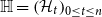 $\mathbb{H}=\left (\mathcal{H}_t\right )_{0\leq t\leq n}$
and
$\mathbb{H}=\left (\mathcal{H}_t\right )_{0\leq t\leq n}$
and
 \begin{equation} \mathcal{H}_{t+1}=\sigma \left (\mathcal{F}_t^{\mathbb{I}},\mathcal{F}_{t+1}^W\right ). \end{equation}
Then,
 \begin{equation} \begin{aligned} Var\left (CDR_{t+1}^{Idios}\right )&=\mathbb{E}^{\mathbb{P}}\big [Var\big (CDR_{t+1}^{Idios}\big|\mathcal{H}_{t+1}\big )\big|\mathcal{F}_t\big]+ Var\big [\mathbb{E}^{\mathbb{P}}\big (CDR_{t+1}^{Idios}\big |\mathcal{H}_{t+1}\big)\big |\mathcal{F}_t\big ]\\ &=\mathbb{E}^{\mathbb{P}}\big [Var\big (CDR_{t+1}^{Idios}\big|\mathcal{H}_{t+1}\big )\big|\mathcal{F}_t\big] \\ &=\mathbb{E}^{\mathbb{P}}\left [Var\left [\sum _{k=1}^{\ell _0}C_{k,t}\cdot \big(\mathbb{E}_t^{\mathbb{P}}[\mathbb{I}_{k,t}]-\mathbb{I}_{k,t}\big)\Bigg |\mathcal{H}_{t+1}\right ]\cdot \eta ^2_{t+1}\Big |\mathcal{F}_t\right ] \\ &=Var\left [\sum _{k=1}^{\ell _0}C_{k,t}\cdot \big(\mathbb{E}_t^{\mathbb{P}}[\mathbb{I}_{k,t}]-\mathbb{I}_{k,t}\big)\right ]\cdot \mathbb{E}\left [\eta ^2_{t+1}\Big |\mathcal{F}_t^W\right ]. \end{aligned} \end{equation}
Fix
 $t$
and define
$t$
and define
 \begin{equation*} Z_t\;:\!=\;\sum _{k=1}^{\ell _t} C_{k,t}\,\mathbb{I}_{k,t}, \end{equation*}
where
 $\{C_{k,t}\}_{k=1}^{\ell _t}$
are
$\{C_{k,t}\}_{k=1}^{\ell _t}$
are
 $\mathcal{F}_t$
-measurable (hence known at time
$\mathcal{F}_t$
-measurable (hence known at time
 $t$
). Assume that, conditionally on
$t$
). Assume that, conditionally on
 $Q_{x+t}$
, the indicators
$Q_{x+t}$
, the indicators
 $\{\mathbb{I}_{k,t}\}_{k=1}^{\ell _t}$
are independent and identically distributed and satisfy
$\{\mathbb{I}_{k,t}\}_{k=1}^{\ell _t}$
are independent and identically distributed and satisfy
 \begin{equation*} \mathbb{I}_{k,t}\mid Q_{x+t}\sim \mathrm{Bernoulli}(Q_{x+t}). \end{equation*}
Set
 $q_{x+t}\;:\!=\;\mathbb{E}_t^{\mathbb{P}}[Q_{x+t}]$
,
$q_{x+t}\;:\!=\;\mathbb{E}_t^{\mathbb{P}}[Q_{x+t}]$
,
 $\sigma ^2_{Q_{x+t}}\;:\!=\;\mathrm{Var}_t(Q_{x+t})$
, and
$\sigma ^2_{Q_{x+t}}\;:\!=\;\mathrm{Var}_t(Q_{x+t})$
, and
 \begin{equation*} \bar C_t^{\,j}\;:\!=\;\frac {1}{\ell _t}\sum _{k=1}^{\ell _t}C_{k,t}^{\,j},\qquad j\in \{1,2\}. \end{equation*}
By the conditional variance decomposition,
 \begin{equation} \mathrm{Var}_t(Z_t) = \mathrm{Var}_t\big (\mathbb{E}_t^{\mathbb{P}}[Z_t \mid Q_{x+t}]\big ) + \mathbb{E}_t^{\mathbb{P}}[\mathrm{Var}_t(Z_t \mid Q_{x+t})]. \end{equation}
Since
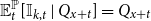 $\mathbb{E}_t^{\mathbb{P}}[\mathbb{I}_{k,t}\mid Q_{x+t}]=Q_{x+t}$
, we have
$\mathbb{E}_t^{\mathbb{P}}[\mathbb{I}_{k,t}\mid Q_{x+t}]=Q_{x+t}$
, we have
 \begin{equation*} \mathbb{E}_t^{\mathbb{P}}[Z_t\mid Q_{x+t}] = \sum _{k=1}^{\ell _t} C_{k,t}\,Q_{x+t} = \ell _t\,\bar C_t^{\,1}\,Q_{x+t}, \end{equation*}
and therefore
 \begin{equation} \mathrm{Var}_t\big (\mathbb{E}_t^{\mathbb{P}}[Z_t\mid Q_{x+t}]\big ) = \ell _t^{2}\,\big(\bar C_t^{\,1} \big) ^{2}\,\sigma ^2_{Q_{x+t}}. \end{equation}
Moreover, by conditional independence and
 $\mathrm{Var}_t(\mathbb{I}_{k,t}\mid Q_{x+t})=Q_{x+t}(1-Q_{x+t})$
,
$\mathrm{Var}_t(\mathbb{I}_{k,t}\mid Q_{x+t})=Q_{x+t}(1-Q_{x+t})$
,
 \begin{equation*} \mathrm{Var}_t(Z_t\mid Q_{x+t}) = \sum _{k=1}^{\ell _t} C_{k,t}^{2}\,Q_{x+t}(1-Q_{x+t}) = \ell _t\,\bar C_t^{\,2}\,Q_{x+t}(1-Q_{x+t}), \end{equation*}
so
 \begin{equation} \mathbb{E}_t^{\mathbb{P}}[\mathrm{Var}_t(Z_t\mid Q_{x+t})] = \ell _t\,\bar C_t^{\,2}\,\mathbb{E}_t^{\mathbb{P}}\big [Q_{x+t}(1-Q_{x+t})\big ]. \end{equation}
Finally,
 \begin{equation*} \mathbb{E}_t^{\mathbb{P}}\big [Q_{x+t}(1-Q_{x+t})\big ] = \mathbb{E}_t^{\mathbb{P}}[Q_{x+t}] - \mathbb{E}_t^{\mathbb{P}}[Q_{x+t}^2] = q_{x+t} - \big (\sigma ^2_{Q_{x+t}} + q_{x+t}^2\big ) = q_{x+t}(1-q_{x+t})-\sigma ^2_{Q_{x+t}}. \end{equation*}
Substituting this into (D.5) and combining with (D.3) and (D.4) yields
 \begin{equation*} \mathrm{Var}_t(Z_t) = \ell _t\,\bar C_t^{\,2}\,q_{x+t}(1-q_{x+t}) +\big (\ell _t^{2} \big(\bar C_t^{\,1} \big)^{2}-\ell _t\,\bar C_t^{\,2}\big )\sigma ^2_{Q_{x+t}}, \end{equation*}
Appendix E. Algorithms
This Appendix outlines the algorithms to evaluate the SCR for Mortality/Longevity Idiosyncratic (Algorithm 1), Trend (Algorithm 2), and Total (Algorithm 3) Demographic risks. In the algorithms, the symbol
 $ \odot$
denotes the Hadamard (element-wise) product between two vectors or matrices.
$ \odot$
denotes the Hadamard (element-wise) product between two vectors or matrices.
SCR for Mortality/Longevity Idiosyncratic risk

SCR for Mortality/Longevity Trend risk

SCR for Total Demographic risk

Appendix F. Simulation burden and numerical stability
To assess the numerical stability of the Monte Carlo procedure and to justify the adopted simulation size, we performed a dedicated convergence analysis of the Solvency Capital Requirement (SCR) estimates. In particular, we investigated the behavior of both the trend and idiosyncratic components of the mortality SCR as the number of simulations increases. For each of the 30 alternative parameter configurations considered in the baseline scenario and sensitivity analysis, we computed the SCR using an increasing number of Monte Carlo replications, up to 10 million simulations. For the trend risk component, convergence was evaluated in terms of the empirical 0.995-quantile of the trend CDR distribution. For the idiosyncratic risk component, we analyzed both the empirical 0.995-quantile of the idiosyncratic CDR distribution and the convergence of the simulated variance to its corresponding analytical value.
Convergence of the simulated variance of the idiosyncratic CDR distribution to its exact analytical value as the number of Monte Carlo simulations increases, for the sensitivity scenarios. Values are normalized with respect to the exact variance.

Convergence of the empirical 0.995-quantile of the idiosyncratic CDR distribution as the number of Monte Carlo simulations increases, for the scenarios considered in the sensitivity analysis. Values are normalized with respect to the estimate obtained with
 $10^7$
simulations.
$10^7$
simulations.

Convergence of the empirical 0.995-quantile of the trend CDR distribution as the number of Monte Carlo simulations increases, for the scenarios considered in the sensitivity analysis. Values are normalized with respect to the estimate obtained with
 $10^7$
simulations.
$10^7$
simulations.

Figure F.1 shows the evolution of the ratio between the variance of the simulated distribution of
 $CDR_{t+1}^{Idios}$
over the exact variance (see formula (4.11)) as a function of the number of simulations
$CDR_{t+1}^{Idios}$
over the exact variance (see formula (4.11)) as a function of the number of simulations
 $m$
for all scenarios. In all cases, the estimates exhibit rapid stabilization as the simulation size increases. Although some variability is present for small sample sizes, particularly below one million simulations, the SCR estimates become essentially flat for larger values of
$m$
for all scenarios. In all cases, the estimates exhibit rapid stabilization as the simulation size increases. Although some variability is present for small sample sizes, particularly below one million simulations, the SCR estimates become essentially flat for larger values of
 $m$
. In particular, the trajectories corresponding to different scenarios converge towards unity, indicating negligible relative deviations once the number of simulations exceeds approximately two million.
$m$
. In particular, the trajectories corresponding to different scenarios converge towards unity, indicating negligible relative deviations once the number of simulations exceeds approximately two million.
A similar convergence pattern is observed for the idiosyncratic and trend SCR components, as shown in Figures F.2 and F.3. In both cases, the estimates stabilize as the number of simulations increases, although convergence is slightly slower than for the variance displayed in Figure F.1. This behavior is expected, since the SCR is based on the estimation of an extreme quantile of the loss distribution, which is inherently more sensitive to Monte Carlo sampling variability than second-order moments such as the variance. Moreover, the convergence of the trend component is comparatively slower than that of the idiosyncratic component. This is mainly due to the additional refitting of the mortality model required in each simulation under trend risk, which introduces an extra source of variability through repeated parameter re-estimation. Nevertheless, a clear stabilization of the trajectories is still observed, with all scenarios exhibiting an approximately flat behavior after about five million simulations, indicating that relative deviations become negligible beyond this threshold.
These results confirm that the Monte Carlo estimator is numerically stable and that reliable SCR estimates can already be obtained with approximately two million simulations. The use of a larger number of simulations in the final implementation is therefore conservative and mainly motivated by the need for accurate estimation of extreme quantiles at the 99.5% level, in particular for the trend CDR component.
Finally, while variance-reduction techniques such as antithetic variates, control variates, or quasi-random sequences could in principle reduce the computational burden, their integration into a bootstrap-based mortality refitting framework is not straightforward. Given the observed stability of the results and the availability of parallel computing, we opted for a standard Monte Carlo approach combined with a large simulation size to ensure robustness of the tail estimates.

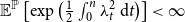


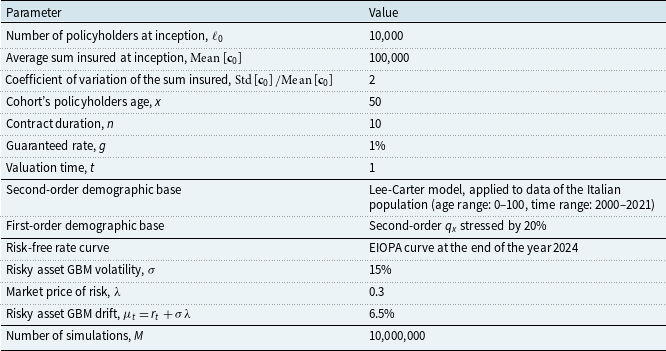
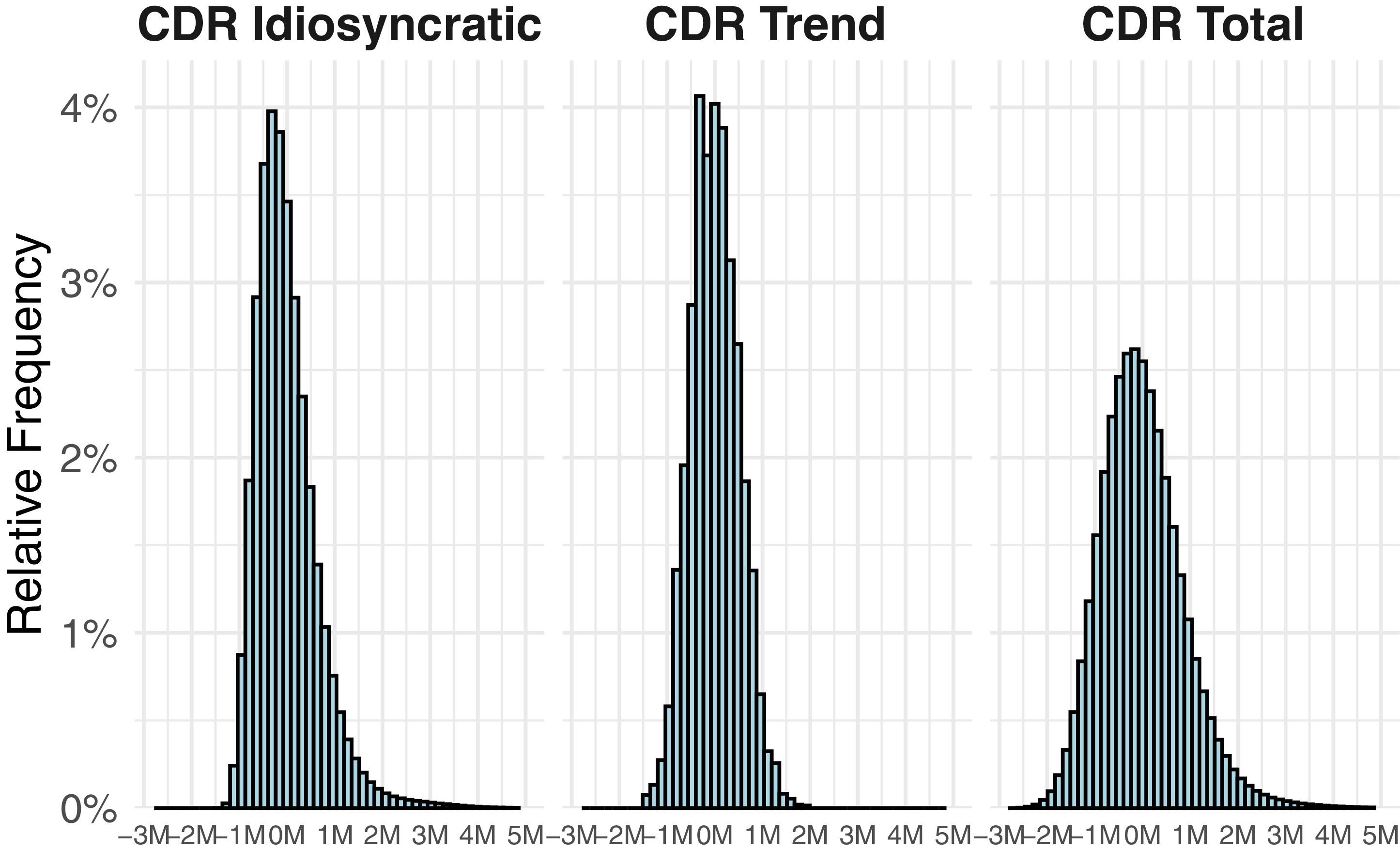
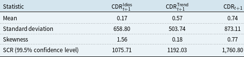
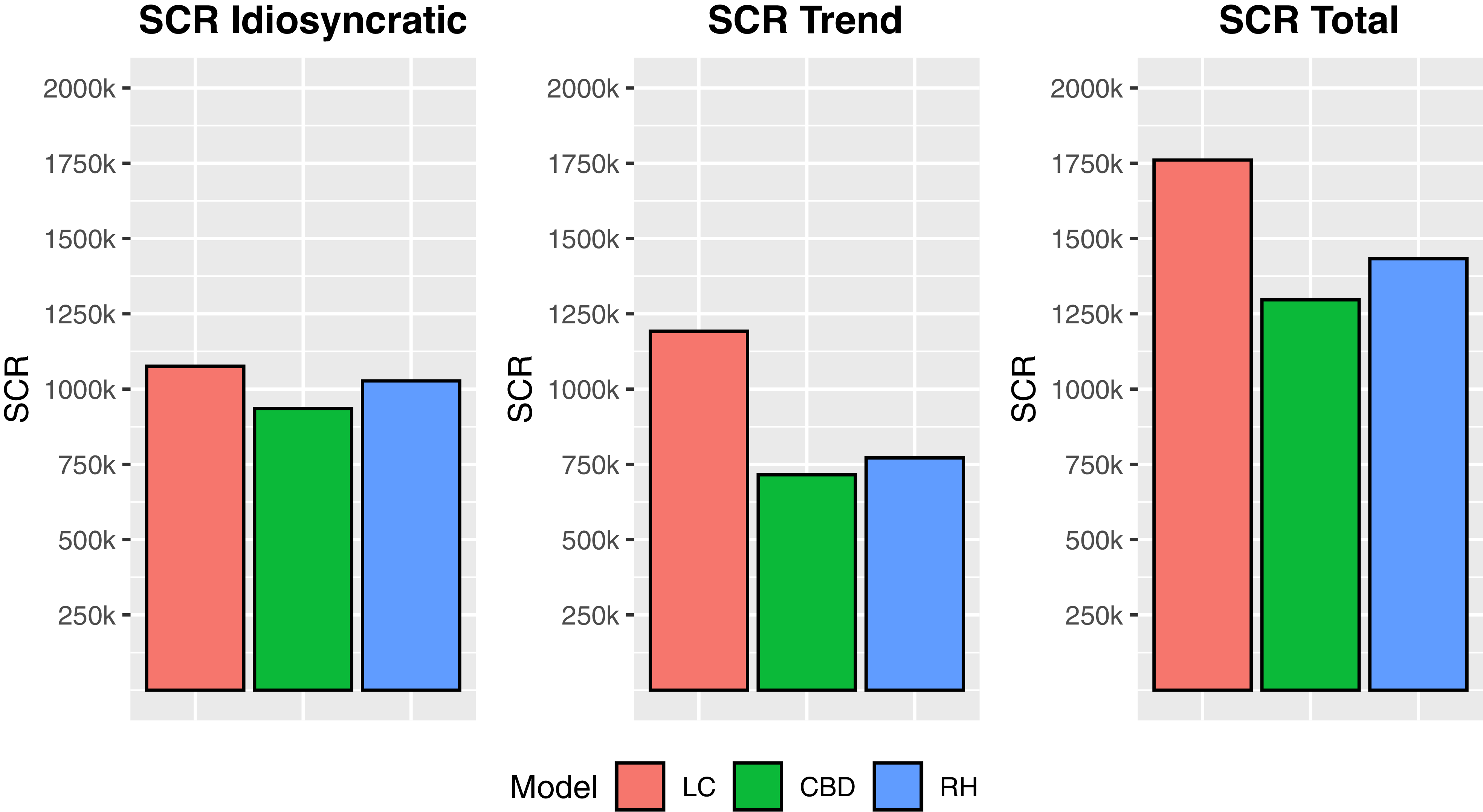


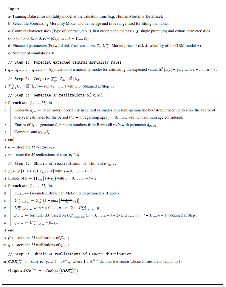
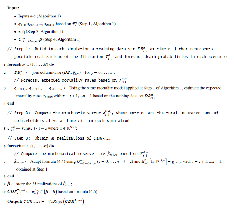
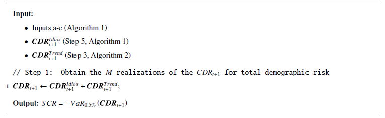
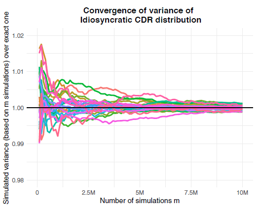
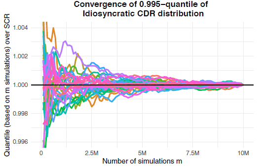

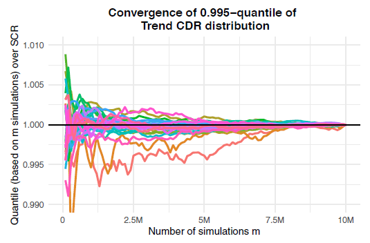


 Open access