


1. Introduction
Earthquakes pose a significant risk to the financial stability of Property and Casualty (P&C) insurers and reinsurers, particularly when they occur in densely populated areas. From an actuarial perspective, their stochastic nature, characterized by unpredictable timing and location, introduces substantial uncertainty into the modeling and pricing of earthquake-related insurance products (U.S. Geological Survey, 2022a). Unlike meteorological perils, the long return periods and low frequency of catastrophic events make historical earthquake loss experience a poor predictor of future risk exposure.
Globally, about 500,000 earthquakes are recorded each year, with roughly 100 strong enough to cause structural damage (U.S. Geological Survey, 2021). The scale of destruction depends heavily on building infrastructure, design standards, and material. For instance, while the 2010 earthquake in Haiti caused nearly 250,000 fatalities, a similarly strong event in New Zealand that same year resulted in no fatalities, largely due to stricter building codes (Wallemacq and House, Reference Wallemacq and House2017).
In Canada, earthquakes occur frequently but are rarely strong enough to cause major damage (NRC, 2019). The west coast, part of the Circum-Pacific seismic belt, also known as the “Ring of Fire,” is particularly active and exposed to high-magnitude events (U.S. Geological Survey, 2022b). In contrast, seismicity in Eastern Canada is driven by regional stress fields and occurs at lower rates. However, the geological properties of Eastern North America allow seismic waves to propagate over much longer distances than in the west, amplifying risk even from moderate earthquakes (U.S. Geological Survey, 2018).
Despite the elevated risk, earthquake insurance uptake remains low in many parts of Canada, particularly in Eastern regions like Québec. Over 70% of Québec’s population resides in seismically active areas, yet only 3.4% of homeowners in Montréal and Québec City purchase earthquake coverage, compared to 65% in Vancouver and Victoria (Swiss Re, 2017). A key deterrent is the structure of earthquake insurance policies, where coverage typically applies only after a high deductible, often calculated as a percentage of the insured value of the property. This means losses must be substantial before a payout occurs, reducing the perceived value of coverage for many policyholders and contributing to under-insurance in high-risk areas.
The Office of the Superintendent of Financial Institutions (OSFI), Canada’s federal insurance and banking regulator, requires insurers to use earthquake models to estimate their probable maximum loss ( $\mathrm{PML}$
), the threshold dollar value of earthquake losses beyond which losses are unlikely, for a 1-in-500 year event, a core component of the minimum capital test (MCT). OSFI (2019) prescribes the following formula for the country-wide earthquake reserve:
$\mathrm{PML}$
), the threshold dollar value of earthquake losses beyond which losses are unlikely, for a 1-in-500 year event, a core component of the minimum capital test (MCT). OSFI (2019) prescribes the following formula for the country-wide earthquake reserve:
 \begin{equation} \text{Country-wide} \mathrm{PML}_{1/500} = \left (\text{East Canada} \ \mathrm{PML}_{1/500}^{1.5} + \text{West Canada} \ \mathrm{PML}_{1/500}^{1.5}\right )^{\frac {1}{1.5}}, \end{equation}
where individual ground-up losses are first reduced by policyholder deductibles at the coverage level, after which losses are aggregated across the portfolio, and the resulting PML is calculated before the application of any reinsurance recoveries. The $\mathrm{PML}_{1/500}$
corresponds to a 1-in-500 year event, representing the
$\mathrm{PML}_{1/500}$
corresponds to a 1-in-500 year event, representing the $99.8^{\text{th}}$
percentile of the distribution of the annual maxima.
$99.8^{\text{th}}$
percentile of the distribution of the annual maxima.
For actuaries, the central difficulty is not simply the stochastic nature of earthquakes, but the practical task of combining diverse data sources into a coherent, reproducible risk assessment framework. This problem affects model calibration, scenario generation, and regulatory capital estimation, especially when catastrophic events are infrequent but potentially severe. Earthquake risk over a space-time window can be written as a compound point process. Let $A\subset \mathbb{R}^2$
be the study region and let
$A\subset \mathbb{R}^2$
be the study region and let $T$
denote a one-year horizon. The aggregate loss is
$T$
denote a one-year horizon. The aggregate loss is
 \begin{equation*} S(A,T)=\sum _{i=1}^{N(A,T)} X_i, \end{equation*}
where $N(A,T)$
is the number of significant earthquake events occurring in
$N(A,T)$
is the number of significant earthquake events occurring in $A\times T$
, and
$A\times T$
, and $X_i$
denotes the total insured loss generated by the
$X_i$
denotes the total insured loss generated by the $i$
-th earthquake event, obtained by aggregating policyholder-level losses across all affected exposures after the application of individual policy deductibles. The precise definition of “significant” is given in Section 2. In this paper we model
$i$
-th earthquake event, obtained by aggregating policyholder-level losses across all affected exposures after the application of individual policy deductibles. The precise definition of “significant” is given in Section 2. In this paper we model $N(A,T)$
using a spatio-temporal point process (STPP), then translate simulated shaking into losses
$N(A,T)$
using a spatio-temporal point process (STPP), then translate simulated shaking into losses $X_i$
via MMI-based damage probability matrices. The insurance risk arising from earthquakes is one of the components of the MCT for federally regulated P&C insurance companies.
$X_i$
via MMI-based damage probability matrices. The insurance risk arising from earthquakes is one of the components of the MCT for federally regulated P&C insurance companies.
While commercial earthquake models, such as AIR and HazCan are widely used for regulatory and internal capital assessment, they are proprietary, costly, and not publicly reproducible (Ulmi et al., Reference Ulmi, Wagner, Wojtarowicz, Bancroft, Hastings, Chow, Rivard, Prieto, Journeay, Struik and Nastev2014). Meanwhile, substantial progress has been made in spatio-temporal modeling of seismic activity, particularly in North America. The Regional Earthquake Likelihood Models project (Field, Reference Field2007) and the Collaboratory for the Study of Earthquake Predictability (Jordan, Reference Jordan2006) have advanced fault-based earthquake forecasting, while model evaluation statistical tests such as the Number-test (N-test), the Likelihood-test (L-test), and the Likelihood-ratio-test (R-test) have helped assess overall model fit (Field, Reference Field2007; Jordan, Reference Jordan2006; Schorlemmer et al., Reference Schorlemmer, Gerstenberger, Wiemer, Jackson and Rhoades2007). These commercial platforms typically combine statistical and physics-based components, including fault rupture modeling, wave propagation, and ground-motion prediction. In contrast, the focus of this paper is on a transparent, fully reproducible, data-driven actuarial framework for loss and capital assessment, which is designed to be complementary to, rather than a substitute for, physics-based seismic hazard models. Publicly documented statistical evaluation tools commonly used in earthquake forecasting, such as the N-test and L-test, primarily assess global model fit and offer limited insight into spatially localized model deficiencies. In this paper, we use spatially resolved residual diagnostics to reveal localized model deficiencies that may not be detectable through aggregate statistics.
Residual-based methods have been proposed for evaluating the goodness-of-fit for STPP models. A common approach involves pixel-based residual methods, where the spatial domain is discretized into a regular grid and the difference between the observed and expected number of events is computed in each pixel, see Baddeley et al. (Reference Baddeley, Turner, Møller and Hazelton2005); Zhuang (Reference Zhuang2006). This yields various types of residuals, such as raw residuals, Pearson residuals, and deviance residuals. These diagnostics provide localized assessments of model fit and help detect areas of under-estimation or over-estimation. However, they can suffer from instability when the expected intensity is close to zero, which is common in seismic applications where many grid cells may contain no events. Moreover, the choice of grid resolution is arbitrary and may not align well with the spatial structure of the data. To overcome these limitations, Bray et al. (Reference Bray, Wong, Barr and Schoenberg2014) introduced Voronoi residual methods, where space is partitioned into irregular, data-driven polygons based on the observed event pattern. Each Voronoi cell contains exactly one observed point and encompasses the region closest to that point. This data-driven partitioning adapts to the local event density, making it particularly useful for modeling inhomogeneous processes. As noted by Bray et al. (Reference Bray, Wong, Barr and Schoenberg2014), standard residual diagnostics, such as Pearson and deviance residuals, can be naturally extended to Voronoi cells, following the general framework by Baddeley et al. (Reference Baddeley, Turner, Møller and Hazelton2005) for pixel-based models.
In this research project, we apply and implement the Voronoi residual diagnostics within a novel actuarial context. Specifically, we apply Pearson and deviance residuals on Voronoi cells to assess the goodness-of-fit of spatio-temporal models for the Canadian significant earthquake point pattern. Moreover, we leverage these diagnostics with an end-to-end simulation framework for earthquake insurance applications. To our knowledge, this represents the first open-source, fully reproducible integration of Voronoi-based residual diagnostics within a simulation-based framework for earthquake insurance risk modeling and capital assessment. We also provide an interactive web application for simulating the occurrence and financial impact of significant earthquakes at user-specified locations. Finally, we review OSFI’s MCT formula in Eq. (1) and propose a potential alternative based on our spatio-temporal model.
The remainder of the paper is organized as follows. Section 2 describes the earthquakes data source used in the analysis. Section 3 presents the simulation methodology, exposure modeling, and an alternative MCT approach for earthquake risk in Canada. Section 4 reports the simulation results and compares our results with other results from simulated earthquakes in the literature, summarizes the outcome of our methodology and compares OSFI’s MCT approach for earthquake risk to our proposed proposal. Section 5 concludes the article. All monetary values are expressed in Canadian dollars unless otherwise stated.
2. Data
This study utilizes a consolidated dataset of significant earthquakes compiled from both historical and instrumental sources and published by the Geological Survey of Canada (GSC) in Open File Report 8285 (Lamontagne et al., Reference Lamontagne, Halchuk, Cassidy and Rogers2018). The dataset spans the period from 1600 to 2017 and includes 172 mainshock events. Each record captures key seismic attributes: origin time, epicentral coordinates (latitude and longitude), depth, magnitude, and regional classification, as well as, when available, indicators of impact such as landslides, tsunamis, structural damage, fatalities, and the maximum Modified Mercalli Intensity (MMI). These attributes form the empirical basis for the subsequent modeling of ground shaking, damage, and insured financial losses.
The dataset distinguishes between pre-instrumental events (1600 to late 19th century), reconstructed from archival documents, felt reports, and paleoseismic evidence, and instrumental events (20th century onward), recorded via seismic networks with higher spatial and temporal precision.
In this study, we restrict attention to the mainshock subset of this catalog and exclude aftershocks. This choice maintains an event-based interpretation of earthquake risk that is consistent with regulatory capital modeling practice, where extreme portfolio losses are typically driven by the mainshock. Including aftershocks as independent loss events would risk double-counting damage to the same exposed portfolio, because aftershocks are conditionally dependent on the mainshock and usually affect the same geographic area. In the proposed framework, earthquake occurrence is first simulated in space and time, while the severity of each event is determined through the ground-shaking module, as described in Section 3.1. As a result, the simulated annual loss distribution reflects the most severe damaging event affecting the portfolio in a given year, regardless of whether it would be classified seismologically as a mainshock or part of an aftershock sequence, as the most severe damaging event is the quantity of interest for solvency capital estimation in an earthquake insurance context.
Figure 1 presents a spatial overview of significant earthquakes in Canada over the study period. An event is considered significant if it satisfies at least one of the following criteria: (i) moment magnitude exceeding 6, or (ii) reported shaking at MMI level V or higher. These thresholds are chosen to focus on events with a realistic potential to trigger earthquake insurance coverage, either through high energy release or through felt shaking severe enough to cause structural damage. Table 8 in Appendix A provides definitions of MMI levels for reference. The distinction between magnitude and intensity is particularly relevant in actuarial contexts: while magnitude quantifies the energy released at the earthquake source, intensity varies by location and better reflects the likelihood and severity of insured losses. MMI is therefore a valuable metric for exposure modeling and geographic pricing in earthquake insurance.
Significant Canadian earthquakes for the period $1600-2017$
. The size and color of the circles are proportionate to the moment magnitude.
$1600-2017$
. The size and color of the circles are proportionate to the moment magnitude.

3. Earthquake simulation methodology
This section explains the methodology used to estimate earthquake-related insurance losses through a simulation-based framework that combines seismic, exposure, and insurance contract data. It also proposes an alternative formulation to Eq. (1) for calculating the MCT for earthquake risk in Canadian P&C insurance companies.
3.1 Calculating exposure and simulating earthquake damage
Seismic risk for a study area is assessed using the following five-step framework:
-
(i) Collecting building inventory and calculating exposure,
-
(ii) Simulating earthquake occurrences in space and time,
-
(iii) Estimating ground shaking intensity,
-
(iv) Estimating Earthquake-Induced Damage Rates, and
-
(v) Estimating seismic losses and insurance claim payments.
The analysis is conducted at the Census Subdivision (CSD) level, Canada’s municipal statistical units, of which there are 5,162 (Statistics Canada, Government of Canada, 2017). Steps (ii) to (v) are summarized in Algorithms 1 and 2.
3.1.1 Collecting building inventory and calculating exposure
Residential exposure is calculated using building counts by type from the 2016 Canadian Census (Statistics Canada, Government of Canada, 2016) and average square footage estimates from the Canadian Housing Statistics Program (Statistics Canada, Government of Canada, 2020a). For each building type, exposure is computed as:
 \begin{equation*}\text{Exposure}=\text{Number of buildings} \times \text{Average area} \times \text{Replacement cost per square foot}.\end{equation*}
Replacement costs are taken from HazCan (Ulmi et al., Reference Ulmi, Wagner, Wojtarowicz, Bancroft, Hastings, Chow, Rivard, Prieto, Journeay, Struik and Nastev2014) and inflated to June 2021 using the Building Construction Price Index (BCPI) (Statistics Canada, Government of Canada, 2020b). To account for regional and estimation uncertainty, we introduce random noise of $\pm 10\%$
to the replacement costs. Content exposure for residential buildings is assumed to be 50% of the structural replacement value (Ulmi et al., Reference Ulmi, Wagner, Wojtarowicz, Bancroft, Hastings, Chow, Rivard, Prieto, Journeay, Struik and Nastev2014; FEMA, 2013). Exposures are then disaggregated by construction material (e.g., wood, steel, concrete) using the general building scheme mapping in HAZUS (Table 5.1 in FEMA (2013)). Exposure is therefore computed separately by building class and construction type, and financial losses are generated using type-specific damage functions applied to the spatially varying shaking intensity. While individual policies are not modeled explicitly, portfolio heterogeneity is captured at the CSD level through building type, construction material, regional variation in floor area, and stochastic variation in replacement costs.
$\pm 10\%$
to the replacement costs. Content exposure for residential buildings is assumed to be 50% of the structural replacement value (Ulmi et al., Reference Ulmi, Wagner, Wojtarowicz, Bancroft, Hastings, Chow, Rivard, Prieto, Journeay, Struik and Nastev2014; FEMA, 2013). Exposures are then disaggregated by construction material (e.g., wood, steel, concrete) using the general building scheme mapping in HAZUS (Table 5.1 in FEMA (2013)). Exposure is therefore computed separately by building class and construction type, and financial losses are generated using type-specific damage functions applied to the spatially varying shaking intensity. While individual policies are not modeled explicitly, portfolio heterogeneity is captured at the CSD level through building type, construction material, regional variation in floor area, and stochastic variation in replacement costs.
Non-residential exposure is estimated indirectly, as no comprehensive database currently exists. We use building permit data (Statistics Canada, Government of Canada, 2020c) and apply annual ratios of non-residential to residential permits, by type (e.g., commercial, institutional), to infer non-residential square footage. Exposure values for these buildings are then calculated similarly, and construction materials and content assumptions follow the HAZUS framework.
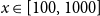
Figure 2 summarizes total calculated exposure per province, with values suppressed to respect the confidentiality of CatIQ’s data, Canada’s Loss and Exposure Indices Provider. See Section 4.1 for details. Western Canada includes British Columbia (BC), Alberta (AB), Saskatchewan (SK), Manitoba (MB), Northwest Territories (NT) and Yukon (YT), and Eastern Canada includes Newfoundland and Labrador (NL), Nova Scotia (NS), Prince Edward Island (PE), New Brunswick (NB), Québec (QC), Ontario (ON), and Nunavut (NU).
Total exposure per province (left) and grouped for Eastern and Western Canada (right). Vertical dashed line separates the two regions.

Figure 3 provides a spatial map of total exposure, building and contents, per square kilometer across CSDs.
Total residential and non-residential exposure (building + contents) per km $^2$
at the CSD level.
$^2$
at the CSD level.

Appendix B provides further details on the estimation of exposure.
3.1.2 Simulating earthquake occurrences in space and time
This section briefly summarizes the STPP and residual diagnostics used as supporting tools within the actuarial earthquake loss and capital modeling framework developed in this paper.
A STPP is a stochastic process that models the occurrence of events in both space and time. Applications include the spread of diseases and pandemics, and natural disasters such as earthquakes, tsunamis, and volcanic eruptions. Point processes are studied thoroughly in time; see Cox and Isham (Reference Cox and Isham1980); Daley and Vere-Jones (Reference Vere-Jones2003) and in space; see Cressie (Reference Cressie2015); Moller and Waagepetersen (Reference Moller and Waagepetersen2003); Diggle (Reference Diggle2013). In seismology, STPPs have been widely used to model earthquake patterns, particularly aftershock sequences; see Ogata (Reference Ogata1998); Zhuang et al. (Reference Zhuang, Ogata and Vere-Jones2002).
An STPP is defined on a subset $S\subseteq \mathbb{R}^2\times \mathbb{R}^{+}$
, where each realization consists of space-time points
$S\subseteq \mathbb{R}^2\times \mathbb{R}^{+}$
, where each realization consists of space-time points $\lbrace (\boldsymbol{x}_i,t_i) \, : \, i =1, \ldots , n \rbrace$
, where
$\lbrace (\boldsymbol{x}_i,t_i) \, : \, i =1, \ldots , n \rbrace$
, where $(\boldsymbol{x}_i,t_i) \in A \times T$
for some known spatial region
$(\boldsymbol{x}_i,t_i) \in A \times T$
for some known spatial region $A$
and temporal period
$A$
and temporal period $T$
, with
$T$
, with $\boldsymbol{x}_i\in A\subset \mathbb{R}^{2}$
representing spatial coordinates (longitude and latitude), and
$\boldsymbol{x}_i\in A\subset \mathbb{R}^{2}$
representing spatial coordinates (longitude and latitude), and $t_i\in T \subset \mathbb{R}^{+}$
the time of occurrence. The first-order properties are described by its spatio-temporal intensity function:
$t_i\in T \subset \mathbb{R}^{+}$
the time of occurrence. The first-order properties are described by its spatio-temporal intensity function:
 \begin{equation*} \lambda (\boldsymbol{x},t)=\lim _{\lvert d\boldsymbol{x}\rvert ,\lvert dt\rvert \to 0}\frac {\mathbb{E}\left [ N(d\boldsymbol{x},dt) \right ]}{\lvert d\boldsymbol{x}\rvert \lvert dt\rvert }, \end{equation*}
where $d\boldsymbol{x}$
represents a small spatial region around the location
$d\boldsymbol{x}$
represents a small spatial region around the location $x$
such that
$x$
such that $\lvert d\boldsymbol{x}\rvert$
is its area,
$\lvert d\boldsymbol{x}\rvert$
is its area, $\lvert dt\rvert$
represents a small time interval containing the time point
$\lvert dt\rvert$
represents a small time interval containing the time point $t$
such that
$t$
such that $\lvert dt\rvert$
is its length, and
$\lvert dt\rvert$
is its length, and $N(d\boldsymbol{x},dt)$
represents the number of events in
$N(d\boldsymbol{x},dt)$
represents the number of events in $d\boldsymbol{x}\times dt$
. Thus,
$d\boldsymbol{x}\times dt$
. Thus, $\lambda (\boldsymbol{x},t)$
represents the expected number of events per unit area per unit of time. If
$\lambda (\boldsymbol{x},t)$
represents the expected number of events per unit area per unit of time. If $\lambda (\boldsymbol{x},t)=\lambda$
is constant, the process is said to be homogeneous. Marginal intensities can be defined by integrating over time or space:
$\lambda (\boldsymbol{x},t)=\lambda$
is constant, the process is said to be homogeneous. Marginal intensities can be defined by integrating over time or space:
 \begin{equation*} \lambda _A(\boldsymbol{x})=\int _T\lambda (\boldsymbol{x},t) dt, \quad \text{and} \quad \lambda _X(t)=\int _A\lambda (\boldsymbol{x},t) d\boldsymbol{x}, \end{equation*}
respectively.
Model fit for STPPs can be assessed using the N-test and L-test introduced by Schorlemmer et al. (Reference Schorlemmer, Gerstenberger, Wiemer, Jackson and Rhoades2007). The N-test compares the observed number of events to simulations from the fitted model, while the L-test evaluates whether the observed log-likelihood exceeds most simulated log-likelihoods. These tests evaluate overall fit but provide limited insight into spatial or temporal misfit.
To provide more granular diagnostics, Baddeley et al. (Reference Baddeley, Turner, Møller and Hazelton2005); Zhuang (Reference Zhuang2006) introduced residual analysis methods based on discretizing the domain into a regular grid of pixels. For a fitted intensity $\hat \lambda (\boldsymbol{x},t)$
, the raw residual for a pixel
$\hat \lambda (\boldsymbol{x},t)$
, the raw residual for a pixel $B_i \in A\times T$
is
$B_i \in A\times T$
is
 \begin{equation*} r^R(B_i) = N(B_i) - \int _{B_i}\hat \lambda (\boldsymbol{x},t) dt d\boldsymbol{x}, \end{equation*}
where $N(B_i)$
is the observed number of events in pixel
$N(B_i)$
is the observed number of events in pixel $B_i$
, which is a measurable set such that
$B_i$
, which is a measurable set such that $B_i\subset A\times T$
, for
$B_i\subset A\times T$
, for $i = 1,\ldots ,m$
, where
$i = 1,\ldots ,m$
, where $m$
is the total number of pre-determined pixels. This compares the total number of observed and estimated points within evenly spaced pixels over a regular grid. Raw residuals can be scaled to improve interpretability. For instance, Pearson residuals rescale the raw residuals to have approximate unit variance, in analogy with Pearson residuals in linear models, i.e.,
$m$
is the total number of pre-determined pixels. This compares the total number of observed and estimated points within evenly spaced pixels over a regular grid. Raw residuals can be scaled to improve interpretability. For instance, Pearson residuals rescale the raw residuals to have approximate unit variance, in analogy with Pearson residuals in linear models, i.e.,
 \begin{equation*} r^P(B_i) = \sum _{(t_j,\boldsymbol{x}_j)\in B_i} \dfrac {1}{\sqrt {\hat \lambda (\boldsymbol{x}_j,t_j)}} - \int _{B_i}\sqrt {\hat \lambda (\boldsymbol{x},t)}dt d\boldsymbol{x}, \end{equation*}
for all $\hat \lambda (\boldsymbol{x}_i,t_i)\gt 0$
. See Baddeley et al. (Reference Baddeley, Turner, Møller and Hazelton2005) for other methods of scaling the gridded residuals and Baddeley et al. (Reference Baddeley, Møller and Pakes2008) for their properties. Analogous to deviances for regression models, Wong and Schoenberg (Reference Wong and Schoenberg2009) propose using deviance residuals to compare two fitted models
$\hat \lambda (\boldsymbol{x}_i,t_i)\gt 0$
. See Baddeley et al. (Reference Baddeley, Turner, Møller and Hazelton2005) for other methods of scaling the gridded residuals and Baddeley et al. (Reference Baddeley, Møller and Pakes2008) for their properties. Analogous to deviances for regression models, Wong and Schoenberg (Reference Wong and Schoenberg2009) propose using deviance residuals to compare two fitted models $\hat \lambda _1$
and
$\hat \lambda _1$
and $\hat \lambda _2$
via their log-likelihood contributions:
$\hat \lambda _2$
via their log-likelihood contributions:
 \begin{align*} r^D(B_i) &= \left (\sum _{(t_j,\boldsymbol{x}_j)\in B_i} \log (\hat \lambda _1(\boldsymbol{x}_j,t_j)) - \int _{B_i} \hat \lambda _1(\boldsymbol{x},t) dt d\boldsymbol{x} \right ) \\ &\quad - \left (\sum _{(t_j,\boldsymbol{x}_j)\in B_i} \log (\hat \lambda _2(\boldsymbol{x}_j,t_j)) - \int _{B_i} \hat \lambda _2(\boldsymbol{x},t) dt d\boldsymbol{x} \right ). \end{align*}
Although pixel-based residuals are informative, they become unstable when the expected number of events per pixel is small, which is a common issue in earthquake modeling. Increasing pixel size to stabilize estimates may distort results in highly inhomogeneous regions.
To address this, Bray et al. (Reference Bray, Wong, Barr and Schoenberg2014) propose Voronoi residual analysis, which partitions the spatial domain using Voronoi tessellations. Each Voronoi cell $C_i$
contains exactly one observed event and comprises all points closer to
$C_i$
contains exactly one observed event and comprises all points closer to $\boldsymbol{x}_i$
than to any other point in the process, for all
$\boldsymbol{x}_i$
than to any other point in the process, for all $i=1, 2, \ldots , n$
. Figure 4 illustrates the Voronoi tessellations of earthquake locations in Figure 1. For more details on Voronoi tessellations and their properties, see Boots et al. (Reference Boots, Okabe and Sugihara1999). For a fitted intensity
$i=1, 2, \ldots , n$
. Figure 4 illustrates the Voronoi tessellations of earthquake locations in Figure 1. For more details on Voronoi tessellations and their properties, see Boots et al. (Reference Boots, Okabe and Sugihara1999). For a fitted intensity $\widehat \lambda (\boldsymbol{x},t)$
, the raw Voronoi residuals are computed as:
$\widehat \lambda (\boldsymbol{x},t)$
, the raw Voronoi residuals are computed as:
 \begin{align*} r^R_V(C_i) &= 1 - \int _{C_i}\hat \lambda (\boldsymbol{x},t) dt d\boldsymbol{x}. \end{align*}
Each residual measures the difference between the observed count (one) and the expected count in cell $C_i$
.
$C_i$
.
Voronoi tessellation of the earthquake locations, shown in Figure 1.

Building on this, we apply Pearson Voronoi residuals, which scale the residuals in analogy to their pixel-based counterparts, defined by:
 \begin{align*} r^P_V(C_i) = \sum _{(t_j,\boldsymbol{x}_j)\in C_i} \dfrac {1}{\sqrt {\hat \lambda (\boldsymbol{x}_j,t_j)}} - \int _{C_i}\sqrt {\hat \lambda (\boldsymbol{x},t)}dt d\boldsymbol{x}. \end{align*}
These residuals are well-defined provided $\hat \lambda (\boldsymbol{x}_i,t_i)\gt 0$
for all
$\hat \lambda (\boldsymbol{x}_i,t_i)\gt 0$
for all $\boldsymbol{x}_i$
and
$\boldsymbol{x}_i$
and $t_i$
, and yield approximately standard-normal values under model adequacy.
$t_i$
, and yield approximately standard-normal values under model adequacy.
To compare two competing models at a local spatial level, we apply the deviance residual concept to Voronoi polygons following the framework of Bray et al. (Reference Bray, Wong, Barr and Schoenberg2014) and Baddeley et al. (Reference Baddeley, Turner, Møller and Hazelton2005). In analogy with linear models, the resulting residuals may be called deviance Voronoi residuals, defined as such:
 \begin{align} r^D_V(C_i) &= \left ( \sum _{(t_j,\boldsymbol{x}_j)\in C_i} \log (\hat \lambda _1(\boldsymbol{x}_j,t_j)) - \int _{C_i} \hat \lambda _1(\boldsymbol{x},t) dt d\boldsymbol{x} \right ) \nonumber \\ &\quad - \left ( \sum _{(t_j,\boldsymbol{x}_j)\in C_i} \log (\hat \lambda _2(\boldsymbol{x}_j,t_j)) - \int _{C_i} \hat \lambda _2(\boldsymbol{x},t) dt d\boldsymbol{x} \right ). \end{align}
Polygons with positive (negative) values indicate regions where $\hat \lambda _1$
(
$\hat \lambda _1$
( $\hat \lambda _2$
) provides a locally improved fit. Summing these residuals across all polygons yields a log-likelihood ratio score that provides a global diagnostic comparison between competing models.
$\hat \lambda _2$
) provides a locally improved fit. Summing these residuals across all polygons yields a log-likelihood ratio score that provides a global diagnostic comparison between competing models.
Now, we apply these residual diagnostics to visually and spatially assess the adequacy of candidate spatio-temporal models as a validation step within the broader earthquake loss and capital simulation framework.
To simulate future events, we construct a spatio-temporal point pattern dataset based on the 137 significant earthquakes in Canada between 1900 and 2017 (Lamontagne et al., Reference Lamontagne, Halchuk, Cassidy and Rogers2018). Events prior to 1900 are excluded due to historical incompleteness that could distort the temporal component of the model. We assume space is continuous and time is discrete (annual), and estimate the spatio-temporal intensity function $\hat {\lambda }(\boldsymbol{x}, t)$
using kernel-based methods (Diggle, Reference Diggle1985). This choice is motivated by the well-established robustness and interpretability of kernel smoothing in spatial and STPP modeling. We also follow a practical approach and assume that the STPP is separable such that
$\hat {\lambda }(\boldsymbol{x}, t)$
using kernel-based methods (Diggle, Reference Diggle1985). This choice is motivated by the well-established robustness and interpretability of kernel smoothing in spatial and STPP modeling. We also follow a practical approach and assume that the STPP is separable such that $\lambda (\boldsymbol{x}, t)$
can be factorized following
$\lambda (\boldsymbol{x}, t)$
can be factorized following
 \begin{equation} \lambda (\boldsymbol{x}, t)=\lambda _{\boldsymbol{x}}(\boldsymbol{x})\lambda _{T}(t), \end{equation}
for all $(\boldsymbol{x},t) \in A\times T.$
This assumption is justified as our interest lies in rare, high-impact events (e.g., the
$(\boldsymbol{x},t) \in A\times T.$
This assumption is justified as our interest lies in rare, high-impact events (e.g., the $\mathrm{PML}_{1/500}$
), where the exact timing is less critical than the spatial distribution of risk exposure. The spatial component
$\mathrm{PML}_{1/500}$
), where the exact timing is less critical than the spatial distribution of risk exposure. The spatial component $\lambda _{\boldsymbol{x}}(\boldsymbol{x})$
is the primary focus for Voronoi residual analysis. Model fitting, simulation, and residual computations are conducted in
R
using the splancs, spatstat, deldir, and stpp packages (Rowlingson and Diggle, Reference Rowlingson and Diggle2022; Baddeley and Turner, Reference Baddeley and Turner2005; Turner, Reference Turner2021; Gabriel et al., Reference Gabriel, Diggle, Rowlingson and Rodriguez-Cortes2022; R Core Team, 2022), along with custom functions developed for Voronoi-based residual diagnostics.
$\lambda _{\boldsymbol{x}}(\boldsymbol{x})$
is the primary focus for Voronoi residual analysis. Model fitting, simulation, and residual computations are conducted in
R
using the splancs, spatstat, deldir, and stpp packages (Rowlingson and Diggle, Reference Rowlingson and Diggle2022; Baddeley and Turner, Reference Baddeley and Turner2005; Turner, Reference Turner2021; Gabriel et al., Reference Gabriel, Diggle, Rowlingson and Rodriguez-Cortes2022; R Core Team, 2022), along with custom functions developed for Voronoi-based residual diagnostics.
To estimate the temporal component of the intensity function, $\lambda _{T}(t)$
, we apply a Gaussian kernel density estimator with bandwidth
$\lambda _{T}(t)$
, we apply a Gaussian kernel density estimator with bandwidth $h_T$
selected via Silverman’s rule-of-thumb (Silverman, Reference Silverman1986), i.e.,
$h_T$
selected via Silverman’s rule-of-thumb (Silverman, Reference Silverman1986), i.e.,
 \begin{equation*}h_T=0.9\alpha n^{-1/5},\end{equation*}
where $\alpha =\min \lbrace \text{sample standard deviation}, \text{sample interquartile range}/1.34\rbrace$
. For the spatial intensity function
$\alpha =\min \lbrace \text{sample standard deviation}, \text{sample interquartile range}/1.34\rbrace$
. For the spatial intensity function $\lambda _{\boldsymbol{x}}(\boldsymbol{x})$
, we use the quartic (biweight) kernel (Diggle, Reference Diggle2013). Bandwidth selection plays a critical role in balancing bias and variance: a smaller bandwidth yields lower bias but higher variance, while a larger bandwidth provides smoother estimates at the cost of increased bias. There is no universally optimal bandwidth, especially for inhomogeneous processes such as earthquakes, which motivates the use of standard data-driven bandwidth selection criteria rather than problem-specific custom estimators. We fit two spatial intensity models using the same kernel but different bandwidths.
$\lambda _{\boldsymbol{x}}(\boldsymbol{x})$
, we use the quartic (biweight) kernel (Diggle, Reference Diggle2013). Bandwidth selection plays a critical role in balancing bias and variance: a smaller bandwidth yields lower bias but higher variance, while a larger bandwidth provides smoother estimates at the cost of increased bias. There is no universally optimal bandwidth, especially for inhomogeneous processes such as earthquakes, which motivates the use of standard data-driven bandwidth selection criteria rather than problem-specific custom estimators. We fit two spatial intensity models using the same kernel but different bandwidths.
-
• Model $H_1$
: bandwidth
$h_1$
minimizes the estimated mean-square error of
$\hat \lambda _{\boldsymbol{x}}(\boldsymbol{x})$
.
$H_1$
: bandwidth
$h_1$
minimizes the estimated mean-square error of
$\hat \lambda _{\boldsymbol{x}}(\boldsymbol{x})$
. -
• Model
$H_2$
: bandwidth
$h_2$
maximizes the leave-one-out likelihood cross-validation score:where
\begin{equation*} LCV(h_2)=\sum _l\log (\lambda _{-l}(\boldsymbol{x}_l))-\int _A \lambda (\boldsymbol{u}) \text d \boldsymbol{u}, \end{equation*}
$\lambda _{-l}(\boldsymbol{x}_l)$
is the intensity estimate at
$\boldsymbol{x}_l$
excluding that point, and
$\lambda (\boldsymbol{u})$
is the smoothed estimate across the domain
$A$
. Baddeley et al. (Reference Baddeley, Rubak and Turner2015) discuss the use of likelihood cross-validation in settings where the point pattern exhibits strong clustering, as is typical for earthquake occurrences. Minimizing the mean-square error is used as the primary criterion for global bandwidth selection, while the leave-one-out likelihood-based bandwidth provides an alternative, data-driven smoothing level. Voronoi residuals are subsequently used for spatial diagnostic validation and local comparison of the competing models.


In addition, we fit a homogeneous Poisson process, denoted Model $P$
, with constant intensity
$P$
, with constant intensity $\lambda (\boldsymbol{x})=\lambda$
for all
$\lambda (\boldsymbol{x})=\lambda$
for all $\boldsymbol{x} \in A$
, to serve as a benchmark for model comparison.
$\boldsymbol{x} \in A$
, to serve as a benchmark for model comparison.
Canada: Raw Voronoi residuals for models $P$
(a),
$P$
(a), $H_1$
(b), and
$H_1$
(b), and $H_2$
(c).
$H_2$
(c).

Figure 5 displays the raw Voronoi residuals for Models $P$
,
$P$
, $H_1$
and
$H_1$
and $H_2$
, plotted on the same color scale. An ideal model produces residuals close to zero. Since raw Voronoi residuals are bounded above by 1 (as each cell contains one observed event), large negative values indicate overestimation by the model. Model
$H_2$
, plotted on the same color scale. An ideal model produces residuals close to zero. Since raw Voronoi residuals are bounded above by 1 (as each cell contains one observed event), large negative values indicate overestimation by the model. Model $P$
clearly underestimates risk in high-seismicity regions of Eastern and Western Canada while overestimating in low-risk zones. This is expected given the homogeneity assumption. Both
$P$
clearly underestimates risk in high-seismicity regions of Eastern and Western Canada while overestimating in low-risk zones. This is expected given the homogeneity assumption. Both $H_1$
and
$H_1$
and $H_2$
perform considerably better, with residuals close to zero across most regions. These visual patterns are confirmed quantitatively by the deviance Voronoi residuals discussed below. Figures 14 and 15 in Appendix C support this conclusion, as do the Pearson Voronoi residual plots in Figures 16–18 therein.
$H_2$
perform considerably better, with residuals close to zero across most regions. These visual patterns are confirmed quantitatively by the deviance Voronoi residuals discussed below. Figures 14 and 15 in Appendix C support this conclusion, as do the Pearson Voronoi residual plots in Figures 16–18 therein.
Deviance Voronoi residuals comparing models $H_1$
vs
$H_1$
vs $H_2$
: Canada (a), Western Canada (b), Eastern Canada (c). Positive values indicate regions where model
$H_2$
: Canada (a), Western Canada (b), Eastern Canada (c). Positive values indicate regions where model $H_1$
has higher local log-likelihood than
$H_1$
has higher local log-likelihood than $H_2$
.
$H_2$
.

To further diagnose spatial differences in model fit, we compute deviance Voronoi residuals (see Eq. (2)), plotting the difference in log-likelihood contributions of models $H_1$
and
$H_1$
and $H_2$
for each Voronoi cell in Figure 6. Model
$H_2$
for each Voronoi cell in Figure 6. Model $H_1$
exhibits consistently better local fit than
$H_1$
exhibits consistently better local fit than $H_2$
in all regions, particularly in low-risk areas such as Northern and Central Canada, where model
$H_2$
in all regions, particularly in low-risk areas such as Northern and Central Canada, where model $H_2$
tends to overpredict seismicity. In high-risk zones, including the Queen Charlotte fault (west) and the St. Lawrence paleo-rift (east),
$H_2$
tends to overpredict seismicity. In high-risk zones, including the Queen Charlotte fault (west) and the St. Lawrence paleo-rift (east), $H_1$
also performs slightly better. The largest deviance residual occurs in the Queen Charlotte fault zone (Figure 6b). The total log-likelihood ratio score between models
$H_1$
also performs slightly better. The largest deviance residual occurs in the Queen Charlotte fault zone (Figure 6b). The total log-likelihood ratio score between models $H_1$
and
$H_1$
and $H_2$
is 210.67, indicating that
$H_2$
is 210.67, indicating that $H_1$
provides a systematically better local fit than
$H_1$
provides a systematically better local fit than $H_2$
. When compared to model
$H_2$
. When compared to model $P$
, the score for
$P$
, the score for $H_1$
is 586.56, while for
$H_1$
is 586.56, while for $H_2$
it is 375.89, indicating that both non-homogeneous models provide substantially improved fit over the homogeneous baseline. Taken together, the mean-square error criterion, likelihood cross-validation, and Voronoi-based residual diagnostics lead us to retain model
$H_2$
it is 375.89, indicating that both non-homogeneous models provide substantially improved fit over the homogeneous baseline. Taken together, the mean-square error criterion, likelihood cross-validation, and Voronoi-based residual diagnostics lead us to retain model $H_1$
as the preferred spatial intensity model for the subsequent earthquake loss and capital simulations.
$H_1$
as the preferred spatial intensity model for the subsequent earthquake loss and capital simulations.
The final fitted spatio-temporal intensity function is obtained by combining the estimated spatial and temporal components:
 \begin{equation*}\hat \lambda (\boldsymbol{x}, t)=\hat \lambda _{\boldsymbol{x}}(\boldsymbol{x}) \cdot \hat \lambda _T(t).\end{equation*}
Earthquake simulations are then conducted using the fitted model via the stpp package in R , allowing the generation of a series of synthetic significant earthquake events over multiple years.
3.1.3 Estimating ground shaking intensity
Seismic hazard in Canada is regularly assessed by the GSC, and updates are reflected in revisions to the National Building Code. Ground shaking intensity, a key input in seismic risk modeling, is typically expressed through attenuation relationships of ground motion indices such as peak ground acceleration (PGA), peak ground velocity, or spectral acceleration. This component represents the physics-informed layer of our otherwise data-driven simulation framework, allowing physical ground-motion processes to directly inform the actuarial loss and capital calculations.
In the proposed framework, earthquake magnitudes are not simulated from a standalone parametric magnitude distribution. Instead, magnitude enters implicitly through the physics-informed ground-shaking component. For each simulated event location, PGA is sampled from a Generalized Pareto Distribution (GPD) fitted to the discrete GSC seismic hazard exceedance points at the nearest grid location. PGA is then converted to MMI using the empirical relationship of Wald et al. (Reference Wald, Quitoriano, Heaton and Kanamori1999). The spatial decay of shaking with distance from the epicenter is modeled using the attenuation relationships of Bakun et al. (Reference Bakun, Johnston and Hopper2003) and Bakun and Wentworth (Reference Bakun and Wentworth1997), which provide an explicit functional link between intensity, magnitude, and source distance.
We use the GSC’s seismic hazard values for firm soil sites from the 2015 National Building Code of Canada (NBCC), covering a grid over Canada and adjacent areas (Halchuk et al., Reference Halchuk, Adams and Allen2015). For each grid point, the mean PGA is available at eight annual exceedance probabilities: 0.02, 0.01375, 0.0100, 0.00445, 0.0021, 0.0010, 0.0005, and 0.000404. A Generalized Pareto Distribution (GPD) is fitted at each grid point to interpolate PGA values across the various return periods. The quantile function for the GPD is provided in Eq. (9) in Appendix D.
For each simulated earthquake epicenter, we identify the nearest PGA grid point and sample a ground motion value using its fitted GPD.
The corresponding MMI level is then estimated using the empirical relationship:
 \begin{equation*}\text{MMI} = 3.66 \log _{10}(\text{PGA}) -1.66,\end{equation*}
with standard error 1.08, for PGA in cm/s $^2$
(Wald et al., Reference Wald, Quitoriano, Heaton and Kanamori1999).
$^2$
(Wald et al., Reference Wald, Quitoriano, Heaton and Kanamori1999).
To model the spatial distribution of shaking, we use attenuation equations developed by Bakun et al. (Reference Bakun, Johnston and Hopper2003) and Bakun and Wentworth (Reference Bakun and Wentworth1997) to estimate moment magnitude as a function of MMI and epicentral distance d (in km):
-
• Eastern Canada (Bakun et al., Reference Bakun, Johnston and Hopper2003):
(4)
\begin{equation} \text{M} = \frac {1}{1.68}\left (\text{MMI} - 1.41 + 0.00345\text{d} + 2.08\log _{10}(\text{d})\right ), \end{equation}
-
• Western Canada (Bakun and Wentworth, Reference Bakun and Wentworth1997):
(5)
\begin{equation} \text{M} = \frac {1}{1.09}\left (\text{MMI} - 5.07 + 3.69\log _{10}(\text{d})\right ), \end{equation}


To ensure consistency with the definition of a significant earthquake (Lamontagne et al., Reference Lamontagne, Halchuk, Cassidy and Rogers2018), only simulated events whose inferred magnitudes, obtained after converting PGA to MMI and applying the attenuation relationships above, exceed $M\gt 6$
are retained for the loss analysis. Since a single earthquake can generate multiple intensity values at varying distances, we construct isoseismal maps, which are contours of equal MMI, by inverting the above relationships to determine the distance d corresponding to each MMI level. Figure 7 shows a sample isoseismal map produced for a simulated earthquake. The concentric shaded regions correspond to different MMI thresholds, illustrating how intensity attenuates with distance from the epicenter of the earthquake. We account for parameter uncertainty by introducing random noise based on the standard errors reported in Bakun and Wentworth (Reference Bakun and Wentworth1997); Bakun et al. (Reference Bakun, Johnston and Hopper2003); Wald et al. (Reference Wald, Quitoriano, Heaton and Kanamori1999). For each MMI level, we identify the affected CSDs and calculate the proportion of each CSD’s area falling within the corresponding isoseismal circle. Algorithm 1 outlines the procedure for simulating an earthquake and generating the corresponding isoseismal maps.
$M\gt 6$
are retained for the loss analysis. Since a single earthquake can generate multiple intensity values at varying distances, we construct isoseismal maps, which are contours of equal MMI, by inverting the above relationships to determine the distance d corresponding to each MMI level. Figure 7 shows a sample isoseismal map produced for a simulated earthquake. The concentric shaded regions correspond to different MMI thresholds, illustrating how intensity attenuates with distance from the epicenter of the earthquake. We account for parameter uncertainty by introducing random noise based on the standard errors reported in Bakun and Wentworth (Reference Bakun and Wentworth1997); Bakun et al. (Reference Bakun, Johnston and Hopper2003); Wald et al. (Reference Wald, Quitoriano, Heaton and Kanamori1999). For each MMI level, we identify the affected CSDs and calculate the proportion of each CSD’s area falling within the corresponding isoseismal circle. Algorithm 1 outlines the procedure for simulating an earthquake and generating the corresponding isoseismal maps.
Isoseismal map for a simulated earthquake, showing the spatial extent of MMI VI–X.

3.1.4 Estimating earthquake-induced damage rates
Earthquakes may result in both financial and non-financial losses. This study focuses on direct financial losses due to physical damage to buildings and their contents. Losses from secondary hazards (e.g., landslides, tsunamis, fire) and non-financial losses (e.g., fatalities, business interruption) are outside the scope of this analysis.
Structural and non-structural damage are modeled separately:
-
• Structural damage refers to the building’s load-bearing components (e.g., walls, roofs).
-
• Non-structural damage is divided into:
-
– Drift-sensitive components (e.g., partitions, cladding),
-
– Acceleration-sensitive components (e.g., mechanical systems, elevators),
-
– Building contents (e.g., furniture, electronics).
-
To quantify damage, we rely on MMI-based damage probability matrices (DPMs), which assign to each building type the probability of being in one of seven defined damage states (e.g., no damage, slight, moderate, destroyed, $\ldots$
) at each MMI level. DPMs were developed by Rojahn et al. (Reference Rojahn and Sharpe1985) and extended to BC by Thibert (Reference Thibert2008) under assumptions of firm ground, regular geometry, and pre-1990 building codes.
$\ldots$
) at each MMI level. DPMs were developed by Rojahn et al. (Reference Rojahn and Sharpe1985) and extended to BC by Thibert (Reference Thibert2008) under assumptions of firm ground, regular geometry, and pre-1990 building codes.
Table 1 shows an illustrative example of a DPM, presenting probabilities by damage state for wood-frame residential buildings at MMI levels VI to XII. Each damage state is associated with a damage factor range, which is the proportion of building value expected to be lost.
DPM for structural damage in wood light frame residential building (Thibert, Reference Thibert2008)

*** represents very small probability values, almost 0.
To quantify damage as a proportion of exposure, we compute the mean damage factor (MDF) for each CSD, building type, and damage component. The MDF is the expected damage percentage at a given MMI level and is computed as the weighted sum of damage factors based on their associated probabilities in the DPM. To introduce simulation variability, damage factors are randomly sampled from their corresponding ranges. Separate MDFs are computed for each damage type (structural (S), acceleration-sensitive (AS) non-structural, drift-sensitive (DS) non-structural, and building contents (BldgC)). These are computed for each CSD-MMI pair and subsequently used to estimate insured losses in Section 3.1(v).
3.1.5 Estimating seismic losses and insurance claim payments
For each simulated event, component losses in CSD $j$
and building class
$j$
and building class $k$
are computed by applying mean damage factors (MDF) to exposures allocated among structural (S), drift-sensitive (DS), acceleration-sensitive (AS), and contents (BldgC) components. Following Onur et al. (Reference Onur, Ventura and Finn2005), exposures are split as 25% to S, 37.5% to DS, and 37.5% to AS; contents exposure is treated separately. Denoting
$k$
are computed by applying mean damage factors (MDF) to exposures allocated among structural (S), drift-sensitive (DS), acceleration-sensitive (AS), and contents (BldgC) components. Following Onur et al. (Reference Onur, Ventura and Finn2005), exposures are split as 25% to S, 37.5% to DS, and 37.5% to AS; contents exposure is treated separately. Denoting
 \begin{equation*} E_{j,k}=\text{building exposure}_{j,k}, \quad C_{j,k}=\text{contents exposure}_{j,k},\end{equation*}
the component losses at MMI level $m$
are
$m$
are
 \begin{align*} L_{j,k,S}^{(m)} &= \mathrm{MDF}_{S,k}^{(m)} \times 0.25\,E_{j,k},\\[3pt] L_{j,k,DS}^{(m)} &= \mathrm{MDF}_{DS,k}^{(m)} \times 0.375\,E_{j,k},\\[3pt] L_{j,k,AS}^{(m)} &= \mathrm{MDF}_{AS,k}^{(m)} \times 0.375\,E_{j,k},\\[3pt] L_{j,k,BldgC}^{(m)}&= \mathrm{MDF}_{BldgC,k}^{(m)} \times C_{j,k}, \end{align*}
and the total loss is
 \begin{equation*} \mathrm{Loss}_{j,k}^{(m)} = L_{j,k,S}^{(m)} + L_{j,k,DS}^{(m)} + L_{j,k,AS}^{(m)} + L_{j,k,BldgC}^{(m)}. \end{equation*}
When a CSD spans multiple MMI levels, each $L_{j,k,*}^{(m)}$
is weighted by the area fraction in level
$L_{j,k,*}^{(m)}$
is weighted by the area fraction in level $m$
.
$m$
.
Table 2 shows market penetration $\pi _j$
, deductible
$\pi _j$
, deductible $d_j$
, and policy limit
$d_j$
, and policy limit $u_j$
used in insurance claim payment calculations. For each CSD:
$u_j$
used in insurance claim payment calculations. For each CSD:
 \begin{align*} \mathrm{Claim}_{j,k} = \begin{cases} 0, & \mathrm{Loss}_{j,k}\le d_j,\\[3pt] \pi _j\,(\mathrm{Loss}_{j,k}-d_j), & d_j\lt \mathrm{Loss}_{j,k}\le u_j,\\[3pt] \pi _j\,(u_j-d_j), & \mathrm{Loss}_{j,k}\gt u_j, \end{cases} \end{align*}
where
 \begin{equation*} d_j = \delta _j \sum _{k} E_{j,k}, \quad u_j = \lambda _j \sum _{k} E_{j,k}, \end{equation*}
with $\delta _j$
and
$\delta _j$
and $\lambda _j$
the deductible and limit percentages at CSD
$\lambda _j$
the deductible and limit percentages at CSD $j$
. Total losses and claims per CSD are
$j$
. Total losses and claims per CSD are
Deductibles, policy limits, and market penetration rates (AIR Worldwide, 2013)

Penetration = fraction of exposed value insured. Deductible and limit = percentage of insured exposure.
 \begin{equation*} \mathrm{Loss}_j = \sum _k \mathrm{Loss}_{j,k}, \quad \mathrm{Claim}_j = \sum _k \mathrm{Claim}_{j,k}. \end{equation*}
Appendix E details Algorithms 1 and 2, which execute the simulation of earthquake events and the calculation of losses and claims. Together, Sections 3.1(ii)–3.1(v) form an end-to-end, fully reproducible actuarial pipeline that links spatio-temporal earthquake occurrence, physics-informed ground shaking, exposure by building type, and insurance loss and claim modeling within a single simulation framework.
3.2 Minimum capital test for earthquake risk
OSFI’s current regulatory capital framework aggregates earthquake risk at broad regional levels (Eastern and Western Canada). In contrast, the proposed framework computes insured losses at a finer spatial resolution (province and CSD level) and introduces a capital aggregation methodology that explicitly incorporates the simulated spatial dependence structure across regions.
OSFI’s MCT aggregation in Eq. (1) is expressed in terms of 1-in-500 gross PMLs for Eastern and Western Canada. In actuarial applications, the PML is defined as a high quantile of the distribution of annual maximum losses. Let $X_1,\ldots ,X_n$
be independent and identically distributed (i.i.d.) annual losses with distribution function
$X_1,\ldots ,X_n$
be independent and identically distributed (i.i.d.) annual losses with distribution function $F$
, and define
$F$
, and define $M_n=\max \{X_1,\ldots ,X_n\}$
. While rule-of-thumb approximations such as
$M_n=\max \{X_1,\ldots ,X_n\}$
. While rule-of-thumb approximations such as $(1+\theta )\,\mathbb{E}[M_n]$
or
$(1+\theta )\,\mathbb{E}[M_n]$
or $\mathbb{E}[M_n]+\theta \sqrt {\mathrm{Var}(M_n)}$
appear in practice (Wilkinson, Reference Wilkinson1982; Kremer, Reference Kremer1990, Reference Kremer1994), we adopt the quantile definition: for small
$\mathbb{E}[M_n]+\theta \sqrt {\mathrm{Var}(M_n)}$
appear in practice (Wilkinson, Reference Wilkinson1982; Kremer, Reference Kremer1990, Reference Kremer1994), we adopt the quantile definition: for small $\epsilon \gt 0$
,
$\epsilon \gt 0$
,
 \begin{equation} \mathbb{P}(M_n \le \mathrm{PML}_\epsilon )=1-\epsilon , \end{equation}
so that $\mathrm{PML}_\epsilon$
is the threshold loss beyond which outcomes are highly unlikely.
$\mathrm{PML}_\epsilon$
is the threshold loss beyond which outcomes are highly unlikely.
Under a peaks-over-threshold framework, exceedances above a high threshold $u$
are approximated by a GPD
$u$
are approximated by a GPD $G_{\xi ,\sigma }$
and the number of exceedances
$G_{\xi ,\sigma }$
and the number of exceedances $N$
is approximately Poisson with rate
$N$
is approximately Poisson with rate $\lambda$
, see Appendix D. The maximum of the
$\lambda$
, see Appendix D. The maximum of the $N$
exceedances is then approximately a generalized extreme value (GEV) distribution
$N$
exceedances is then approximately a generalized extreme value (GEV) distribution $H_{\xi ,\mu ,\psi }$
with
$H_{\xi ,\mu ,\psi }$
with $\mu =\frac {\sigma }{\xi }(\lambda ^\xi -1)$
and
$\mu =\frac {\sigma }{\xi }(\lambda ^\xi -1)$
and $\psi =\sigma \lambda ^\xi$
(Cebrián et al., Reference Cebrián, Denuit and Lambert2003). Solving Eq. (6) yields
$\psi =\sigma \lambda ^\xi$
(Cebrián et al., Reference Cebrián, Denuit and Lambert2003). Solving Eq. (6) yields
 \begin{equation} \mathrm{PML}_\epsilon = u + \frac {\sigma }{\xi }\left [\left ( -\frac {\lambda }{\ln (1-\epsilon )}\right )^{\xi } -1 \right ]. \end{equation}
Inspired by the Solvency II framework of the European Commission (2015), we propose aggregating PMLs from all Canadian provinces and territories via a variance-covariance structure that reflects cross-regional dependence of insured earthquake losses:
 \begin{equation} \text{Country-wide} \ \mathrm{PML}_{1/500} = \sqrt {\sum _{r,s}\text{CorrEQ}_{r,s}\times \mathrm{PML}_{1/500,r} \times \mathrm{PML}_{1/500,s}}, \end{equation}
where $\text{CorrEQ}_{r,s}$
denotes the correlation between simulated annual insured losses in regions
$\text{CorrEQ}_{r,s}$
denotes the correlation between simulated annual insured losses in regions $r$
and
$r$
and $s$
, and
$s$
, and $\mathrm{PML}_{1/500,r}$
and
$\mathrm{PML}_{1/500,r}$
and $\mathrm{PML}_{1/500,s}$
are the corresponding regional PMLs calculated net of policyholder deductibles and prior to the application of any reinsurance recoveries.
$\mathrm{PML}_{1/500,s}$
are the corresponding regional PMLs calculated net of policyholder deductibles and prior to the application of any reinsurance recoveries. $\sum _{r,s}$
denotes the double sum over all regions.
$\sum _{r,s}$
denotes the double sum over all regions.
For each region $r$
, we compute
$r$
, we compute $\mathrm{PML}_{1/500,r}$
by (a) the empirical
$\mathrm{PML}_{1/500,r}$
by (a) the empirical $(1-1/500)$
quantile of simulated annual maxima, and (b) the EVT estimate obtained by inserting
$(1-1/500)$
quantile of simulated annual maxima, and (b) the EVT estimate obtained by inserting $\hat {\mu },\hat {\sigma },\hat {\xi },\hat {\lambda }$
into Eq. (7). The correlation matrix
$\hat {\mu },\hat {\sigma },\hat {\xi },\hat {\lambda }$
into Eq. (7). The correlation matrix $\text{CorrEQ}$
is estimated from simulated annual insured losses, including zeros for years with no earthquake damage. Concurrent impacts from a single event naturally induce positive dependence across provinces. We examine Pearson correlation, Kendall’s
$\text{CorrEQ}$
is estimated from simulated annual insured losses, including zeros for years with no earthquake damage. Concurrent impacts from a single event naturally induce positive dependence across provinces. We examine Pearson correlation, Kendall’s $\tau$
, and Kendall’s
$\tau$
, and Kendall’s $\tau$
for zero-inflated continuous variables (Pimentel et al., Reference Pimentel, Niewiadomska-Bugaj and Wang2015).Footnote 1
$\tau$
for zero-inflated continuous variables (Pimentel et al., Reference Pimentel, Niewiadomska-Bugaj and Wang2015).Footnote 1
4. Results
This section presents three sets of findings. First, we benchmark the exposure estimates produced by our methodology against CatIQ’s insured exposure indices, see Section 4.1. Secondly, we externally validate the simulated financial losses and insurance claim payments by comparison with Onur et al. (Reference Onur, Ventura and Finn2005), see Section 4.2. Third, we report the earthquake simulation outputs in detail, including distributional summaries and PML estimates, see Section 4.3.
4.1 Comparison of exposure values
CatIQ aggregates insurer-reported exposure and loss data for the Canadian market via a subscription platform. We benchmark our insured exposure estimates against CatIQ’s 2020 exposures by applying the market penetration rates in Table 2 to the replacement-cost exposures constructed in Section 3.1. All amounts are expressed in June 2021 CAD. To respect CatIQ confidentiality, the $y$
-axis values in Figure 8 are suppressed.
$y$
-axis values in Figure 8 are suppressed.
Overall, the residential exposures produced by our public-data methodology are of comparable magnitude to CatIQ’s insurer-reported values, which is adequate for the purposes of this open-source risk assessment framework. Larger discrepancies arise for non-residential exposures, reflecting (i) the absence of a comprehensive national inventory for non-residential buildings, (ii) our reliance on building-permit ratios to scale from residential to non-residential stock, and (iii) mapping assumptions to HAZUS occupancy classes; see Section 3.1.
Benchmarking calculated insured exposure, Section 3.1, against CatIQ’s insurer-reported exposure, shown in June 2021 CAD. The $y$
-axis is suppressed to maintain CatIQ data confidentiality.
$y$
-axis is suppressed to maintain CatIQ data confidentiality.

4.2 Comparison with prior earthquake loss studies
We externally validate our direct loss estimates by comparing them with Onur et al. (Reference Onur, Ventura and Finn2005), who evaluated citywide impacts for Victoria and Vancouver under a uniform shaking scenario of MMI VIII. Their study reports total monetary losses of $\$430$
million for the City of Victoria and
$\$430$
million for the City of Victoria and $\$3.5$
billion for the city of Vancouver in 2001 CAD. Inflating via the BCPI (Statistics Canada, Government of Canada, 2020b) to June 2021 yields
$\$3.5$
billion for the city of Vancouver in 2001 CAD. Inflating via the BCPI (Statistics Canada, Government of Canada, 2020b) to June 2021 yields $\$835$
million and
$\$835$
million and $\$6.8$
billion, respectively.
$\$6.8$
billion, respectively.
Under the same MMI VIII assumption, our methodology produces direct losses of $\$941$
million for Victoria and
$\$941$
million for Victoria and $\$5.73$
billion for Vancouver. Relative to the BCPI-inflated values from Onur et al. (Reference Onur, Ventura and Finn2005), this corresponds to a difference of approximately + 12.7% for Victoria and
$\$5.73$
billion for Vancouver. Relative to the BCPI-inflated values from Onur et al. (Reference Onur, Ventura and Finn2005), this corresponds to a difference of approximately + 12.7% for Victoria and $-15.7\%$
for Vancouver.
$-15.7\%$
for Vancouver.
Differences arise from several sources: (i) Onur et al. (Reference Onur, Ventura and Finn2005) exclude content losses, whereas our framework models contents explicitly, and (ii) construction cost inputs differ: local contractor estimates in Onur et al. (Reference Onur, Ventura and Finn2005) vs. HAZUS-based replacement costs scaled by BCPI in our approach. Taken together, these factors plausibly explain the direction and magnitude of divergences while remaining consistent at the order-of-magnitude level across both cities. We therefore view this comparison as an external reasonableness check on the loss module.
4.3 Simulation results
We report simulation outputs from our earthquake model and compare Canada-wide PMLs obtained via the proposed aggregation in Eq. (8) with those from OSFI’s formula in Eq. (1).
We simulate 100,000 years of seismic activity using the procedure in Section 3, a horizon chosen to reduce Monte Carlo variability.Footnote 2 Table 3 summarizes the proportion of years with at least one significant event and the proportion with damage-inducing events.
Proportion of simulated years with significant earthquakes and with damage-inducing significant earthquakes, based on 100,000 simulated years

Figure 9 displays a representative 200-year sample of simulated events. The spatial distribution and magnitudes closely resemble the historical pattern in Figure 1.
Two hundred simulated years of earthquakes. Circle size and color are proportional to moment magnitude.

Using the exposure framework in Section 3.1 and the simulation procedures in Algorithms 1 and 2, we compute direct financial losses and insured claim payments at the CSD level for each simulated event. Figure 10 shows the conditional expectations, given that an earthquake occurs in the CSD, of losses and claims, while Figures 11 and 12 show province-level summaries. CSDs outside active seismic zones have conditional expectations equal to zero. At the provincial scale, conditional expected losses increase as exposure increases, see Figure 2. By contrast, conditional expected claims depend not only on exposure but also on market penetration and contract terms such as deductibles and limits, so their cross-provincial ranking can differ from the ranking by exposure. In Eastern Canada, higher non-residential penetration rates translate into relatively larger conditional claims for commercial/industrial classes. Finally, East–West differences are consistent with attenuation characteristics: for a magnitude 6 event, MMI VI can extend to approximately 200 km in Eastern Canada but only about 33 km in Western Canada, see (U.S. Geological Survey, 2018).
Average financial losses (a) and insurance claims (b) by CSD, conditional on an earthquake occurrence, based on 100,000 simulated years.

Average financial losses per province, conditional on an earthquake occurrence, based on 100,000 simulated years. The vertical dashed line separates Eastern and Western provinces.

For aggregation via Eq. (8), we estimate cross-provincial dependence using simulated annual insured losses. Table 4 shows Pearson correlations for financial losses. Additional results for Kendall’s $\tau$
and claims correlations appear in Tables 10, 11, and 12 in Appendix F. As expected, dependence is strongest within regional clusters, such as QC-ON and BC with neighboring territories, reflecting concurrent impacts from large events.
$\tau$
and claims correlations appear in Tables 10, 11, and 12 in Appendix F. As expected, dependence is strongest within regional clusters, such as QC-ON and BC with neighboring territories, reflecting concurrent impacts from large events.
Pearson’s correlation of the simulated financial losses between Canadian provinces and territories, based on 100,000 years of simulated earthquakes

Average insurance claims per province, conditional on an earthquake occurrence, based on 100,000 simulated years. The vertical dashed line separates Eastern and Western provinces.

Table 5 reports GPD and Poisson parameter estimates for exceedances above threshold $u$
, where
$u$
, where $u$
is chosen as the 0.95 quantile, or 0.90 for provinces when exceedances are sparse, with standard errors. Diagnostic plots (not shown) support GPD adequacy.
$u$
is chosen as the 0.95 quantile, or 0.90 for provinces when exceedances are sparse, with standard errors. Diagnostic plots (not shown) support GPD adequacy.
Parameter estimates for the fitted GPD and Poisson model based on 100,000 simulated years

Tables 6 and 7 present provincial PML $_{1/x}$
values for
$_{1/x}$
values for $x\in \{100,250,500,750,1000\}$
using both the empirical quantiles of simulated annual maxima (“Simulated”) and the EVT formula in Eq. (7) (“Estimated”). Additionally, Canada-wide PMLs are reported under OSFI’s Eq. (1) and under Eq. (8) using Pearson’s correlation and Kendall’s
$x\in \{100,250,500,750,1000\}$
using both the empirical quantiles of simulated annual maxima (“Simulated”) and the EVT formula in Eq. (7) (“Estimated”). Additionally, Canada-wide PMLs are reported under OSFI’s Eq. (1) and under Eq. (8) using Pearson’s correlation and Kendall’s $\tau$
. Simulated and EVT-estimated results are closely aligned, confirming model fit. We observe that the correlation-based aggregation in Eq. (8) yields values comparable to OSFI’s approach, and the results using Kendall’s
$\tau$
. Simulated and EVT-estimated results are closely aligned, confirming model fit. We observe that the correlation-based aggregation in Eq. (8) yields values comparable to OSFI’s approach, and the results using Kendall’s $\tau$
are more conservative than those using Pearson correlation.
$\tau$
are more conservative than those using Pearson correlation.


Figure 13 compares Canada-wide PML $_{1/x}$
curves for losses and claims. For financial losses, Eq. (8) exceeds OSFI’s values across
$_{1/x}$
curves for losses and claims. For financial losses, Eq. (8) exceeds OSFI’s values across $x\in [100,1000]$
, with the gap widening as tail depth increases. At
$x\in [100,1000]$
, with the gap widening as tail depth increases. At $x=500$
, Pearson-based aggregation is roughly
$x=500$
, Pearson-based aggregation is roughly $\$27\mathrm{B}$
above OSFI and Kendall-based aggregation is about
$\$27\mathrm{B}$
above OSFI and Kendall-based aggregation is about $\$51\mathrm{B}$
higher. This is because the proposed formula reflects the strong dependence between QC and ON and the shared impact from large Eastern events and broader isoseismal footprints. However, for insurance claims, Eq. (8) with Pearson correlation is very close to OSFI, while Kendall’s
$\$51\mathrm{B}$
higher. This is because the proposed formula reflects the strong dependence between QC and ON and the shared impact from large Eastern events and broader isoseismal footprints. However, for insurance claims, Eq. (8) with Pearson correlation is very close to OSFI, while Kendall’s $\tau$
produces modestly higher values, about
$\tau$
produces modestly higher values, about $\$3\mathrm{B}$
at
$\$3\mathrm{B}$
at $x=500$
. Adoption of Eq. (8) with Pearson correlation would therefore yield a smooth transition relative to current practice.
$x=500$
. Adoption of Eq. (8) with Pearson correlation would therefore yield a smooth transition relative to current practice.


5. Discussion
Canada’s seismic risk is material because sizeable urban populations lie within active zones in both the East and the West. Quantifying the associated financial impact is therefore relevant for insurance companies, reinsurers, regulators, and public policy.
This paper makes three contributions. First, we develop an open, reproducible actuarial framework that links spatio-temporal earthquake occurrence, physics-informed ground shaking, exposure by building type, and explicit insurance terms to simulate direct financial losses and insured claims using publicly available data sources. Second, within this framework, we demonstrate how Voronoi-based raw, Pearson, and deviance residual diagnostics can be used as spatially resolved tools to assess local model adequacy and to check the consistency between the fitted earthquake occurrence model and the resulting financial loss and insurance claim estimates. Third, we propose a correlation-based aggregation of provincial/territorial PMLs, by relying on variance-covariance formulas, as a transparent alternative to the current two-region OSFI aggregation.
Our simulations of 100,000 years of earthquakes indicate that the correlation-based aggregation produces Canada-wide PMLs comparable to OSFI’s formula for insured claims, while yielding higher values for total losses due to stronger cross-provincial dependence in large Eastern events. The framework also quantifies the coverage gap. For example, in Québec the 1-in-500 year financial loss is approximately $\$180$
billion, while the corresponding insured claims are about
$\$180$
billion, while the corresponding insured claims are about $\$28$
billion under current market penetration and terms, leaving a substantial residual burden on households and governments. Covering
$\$28$
billion under current market penetration and terms, leaving a substantial residual burden on households and governments. Covering $\$152$
billion would double the planned total expenditures for 2021–2022 (Gouvernement du Québec, 2021) and lead to a major deficit. This amount represents considerable government expenditures, for example, it is nine-fold the budgeted COVID-19 support and recovery measures for the years 2020–2024. Similar gaps appear in other provinces, particularly in Eastern Canada where penetration for residential cover remains low.
$\$152$
billion would double the planned total expenditures for 2021–2022 (Gouvernement du Québec, 2021) and lead to a major deficit. This amount represents considerable government expenditures, for example, it is nine-fold the budgeted COVID-19 support and recovery measures for the years 2020–2024. Similar gaps appear in other provinces, particularly in Eastern Canada where penetration for residential cover remains low.
Several limitations are noteworthy. Non-residential exposures are approximated from building-permit ratios due to the absence of a comprehensive national inventory, which introduces uncertainty in commercial and industrial losses. The intensity model relies on separability and on historical data with varying completeness, and although this is appropriate for our PML focus, potential non-stationarity and the exclusion of explicit aftershock triggering require further study. In the present framework, losses are simulated on an annual basis, so the loss distribution reflects the most severe event affecting the portfolio in a given year, regardless of whether it is classified as a mainshock or aftershock, which is the relevant measure for solvency capital estimation. Results are also sensitive to policy parameters including deductibles and limits and to insurance penetration, so inputs should be refreshed as market conditions evolve. Future work should incorporate richer exposure inventories such as municipal assessment rolls, extend the hazard module to include secondary perils and site amplification, model temporal non-stationarity, and explore dependence structures beyond linear correlation with attention to tail dependence within the aggregation formula. Notwithstanding these caveats, the proposed reproducible approach offers a practical actuarial toolkit for pricing, capital assessment, and stress testing of Canadian earthquake risk.
Supplementary material
The supplementary material for this article can be found at https://doi.org/0.1017/S1748499526100293
Acknowledgements
This research was supported in part by the Society of Actuaries’ James C. Hickman Scholar Program. The second author acknowledges the support of the Natural Sciences and Engineering Research Council of Canada RGPIN-2016-04114 and the HEC Montreal Foundation. The third author recognizes the support of the Natural Sciences and Engineering Research Council of Canada RGPIN-2015-05447.
Competing interests
The author(s) declare none.
Appendix A. Modified Mercalli intensity definitions
Modified Mercalli intensity definitions (Wood and Neumann, Reference Wood and Neumann1931)

Appendix B. Collection of building inventory and calculation of exposure
We define:
-
• Total square footage = # units of a building type
$\times$
average square footage of that type of unit -
• Building exposure = Total square footage
$\times$
Mean replacement cost per square footage -
• Building content exposure = Building exposure
$\times$
% contents value.


We next describe the data sources and imputations used for building inventory and replacement costs.
Residential d wellings
Counts by residential class are taken from Statistics Canada, Government of Canada (2016), and mapped to HAZUS occupancy codes using Table C.4 in Ulmi et al. (Reference Ulmi, Wagner, Wojtarowicz, Bancroft, Hastings, Chow, Rivard, Prieto, Journeay, Struik and Nastev2014). Average living area (sq.ft.) by class and CSD is from the Canadian Housing Statistics Program (CHSP) Statistics Canada, Government of Canada (2020a), with data available for BC, ON, NS, NB. Missing CSD-level square footage is imputed using the CSD within the same province with the closest median household income, obtained from Statistics Canada, Government of Canada (2016). If both are missing, we use the province’s weighted average, where the weights are the number of houses in each CSD. For provinces without CHSP square footage, proxy values are assigned by using the square footage values of a CSD that has the nearest household income values, where the provinces are matched as follows:
-
• ON square footage is used for QC, MB, and NU.
-
• NB square footage is used for NL and PE.
-
• BC square footage is used for SK, AB, YT, and NT.
For dwelling types lacking square footage, we assume that an “other single-attached” house has the same square footage as a “single-detached” house and an “apartment or flat in a duplex” has the same square footage as a “Semi-detached” house.
Building replacement costs by HAZUS occupancy are from Ulmi et al. (Reference Ulmi, Wagner, Wojtarowicz, Bancroft, Hastings, Chow, Rivard, Prieto, Journeay, Struik and Nastev2014), which was originally obtained from the RSMeans, and are inflated to June 2021 using the Building Construction Price Index (BCPI) (Statistics Canada, Government of Canada, 2020b). BCPI is reported for selected census metropolitan areas (CMA), thus we apply each CMA’s rate to its province. For provinces/territories without BCPI, we adopt the smallest observed rate, which is that of Edmonton in AB, and for NB, we use Halifax, NS. Contents values for residential classes are set at 50% of building replacement cost (Ulmi et al., Reference Ulmi, Wagner, Wojtarowicz, Bancroft, Hastings, Chow, Rivard, Prieto, Journeay, Struik and Nastev2014; FEMA, 2013). Exposures by HAZUS occupancy are disaggregated into construction types (wood, concrete, steel, masonry, etc.) using the general building scheme in Table 5.1 of FEMA (2013).
Non-residential d wellings
In the absence of a national inventory, we scale from residential exposure using Statistics Canada building permits (Statistics Canada, Government of Canada, 2020c). We compute average annual ratios of institutional/governmental, commercial, and industrial permits to residential permits over 2011-2019 and apply these ratios to obtain non-residential exposure totals by region. Table 9 shows the mapping from permits labels to HAZUS occupancy codes. As for residential, we convert occupancy to construction types using Table 5.1 of FEMA (2013). Contents values for non-residential classes follow the percentages in FEMA (2013).
Conversion from statistics Canada classification to HAZUS occupancy codes for non-residential buildings

Appendix C. Residual analysis of the fitted STPP models
This appendix presents Voronoi residual diagnostics for three intensity models: the homogeneous Poisson model $P$
and two kernel-smoothed inhomogeneous models
$P$
and two kernel-smoothed inhomogeneous models $H_1$
and
$H_1$
and $H_2$
. We show raw and Pearson residual maps for Canada and by region. All panels use a common color scale to enable visual comparison.
$H_2$
. We show raw and Pearson residual maps for Canada and by region. All panels use a common color scale to enable visual comparison.
Western Canada: Raw Voronoi residuals for models $P$
(a),
$P$
(a), $H_1$
(b), and
$H_1$
(b), and $H_2$
(c).
$H_2$
(c).

Eastern Canada: Raw Voronoi residuals for models $P$
(a),
$P$
(a), $H_1$
(b), and
$H_1$
(b), and $H_2$
(c).
$H_2$
(c).

Canada: Pearson Voronoi residuals for models $P$
(a),
$P$
(a), $H_1$
(b), and
$H_1$
(b), and $H_2$
(c).
$H_2$
(c).

Western Canada: Pearson Voronoi residuals for models $P$
(a),
$P$
(a), $H_1$
(b), and
$H_1$
(b), and $H_2$
(c).
$H_2$
(c).

Eastern Canada: Pearson Voronoi residuals for models $P$
(a),
$P$
(a), $H_1$
(b), and
$H_1$
(b), and $H_2$
(c).
$H_2$
(c).

Appendix D. Extreme value theory
Extreme value theory (EVT) is a branch in statistics that characterizes tail behavior of distributions (Coles, Reference Coles2001). Two principal approaches are used: (i) block maxima, which models maxima of i.i.d. observations within successive blocks, and (ii) peaks over threshold, which models exceedances above a high threshold $u$
. The asymptotics-based Generalized Pareto Distribution (GPD) for the exceedances is fitted to extreme values of peak ground acceleration (PGA) obtained from the seismic hazard curves to enable extreme ground motion simulations.
$u$
. The asymptotics-based Generalized Pareto Distribution (GPD) for the exceedances is fitted to extreme values of peak ground acceleration (PGA) obtained from the seismic hazard curves to enable extreme ground motion simulations.
D.1 Distribution of the maxima
The limiting distribution of block maxima is given in the following theorem:
Theorem D.1 (Fisher-Tippett-Gnedenko (Fisher and Tippett, Reference Fisher and Tippett1928)). Let $X_1,\ldots ,X_n$
be a sequence of i.i.d. with distribution function
$X_1,\ldots ,X_n$
be a sequence of i.i.d. with distribution function $F$
, and
$F$
, and $M_n=\max \{X_1,\ldots ,X_n\}$
. If there exist norming constants
$M_n=\max \{X_1,\ldots ,X_n\}$
. If there exist norming constants $a_n\in \mathbb{R}$
,
$a_n\in \mathbb{R}$
, $b_n\gt 0$
for all
$b_n\gt 0$
for all $n\in \mathbb{N}$
and some non-degenerate distribution function
$n\in \mathbb{N}$
and some non-degenerate distribution function $H$
such that
$H$
such that $\frac {M_n-a_n}{b_n}\xrightarrow {d}H$
, then
$\frac {M_n-a_n}{b_n}\xrightarrow {d}H$
, then $H$
is, up to location and scale, one of: Fréchet, Gumbel, or Weibull.
$H$
is, up to location and scale, one of: Fréchet, Gumbel, or Weibull.
Following Von Mises (Reference Von Mises1954); Jenkinson (Reference Jenkinson1955), these families are unified by the generalized extreme value (GEV) distribution.
Definition D.1 (Generalized Extreme Value Distribution). The distribution function of a GEV is given by
 \begin{align*} H_{\xi }(x)&= \begin{cases} \exp \left \lbrace -\left (1+\xi x \right )^{-\frac {1}{\xi }}\right \rbrace , &\ \ \xi \neq 0,\\ \exp \left \lbrace -\exp ({-}x)\right \rbrace , &\ \ \xi =0,\\ \end{cases} \end{align*}
where $1+\xi x\gt 0$
. A three-parameter family is obtained by defining
$1+\xi x\gt 0$
. A three-parameter family is obtained by defining $H_{\xi ,\mu ,\sigma } \, :\!= \,H_{\xi }\left ( \frac {x-\mu }{\sigma } \right )$
for a location parameter
$H_{\xi ,\mu ,\sigma } \, :\!= \,H_{\xi }\left ( \frac {x-\mu }{\sigma } \right )$
for a location parameter $\mu \in \mathbb{R}$
, a scale parameter
$\mu \in \mathbb{R}$
, a scale parameter $\sigma \gt 0$
, and a shape parameter
$\sigma \gt 0$
, and a shape parameter $\xi \in \mathbb{R}$
.
$\xi \in \mathbb{R}$
.
D.2 Distribution of the exceedances
Rather than one maximum per block, the peaks-over-threshold method uses all exceedances above a high threshold $u$
.
$u$
.
Definition D.2 (Excess Distribution over threshold $\boldsymbol{u}$
). For a random variable
$\boldsymbol{u}$
). For a random variable $X$
with distribution function
$X$
with distribution function $F$
and right endpoint
$F$
and right endpoint $x_F\le \infty$
, the excess cdf is
$x_F\le \infty$
, the excess cdf is
 \begin{equation*} F_u(x)=\mathbb{P}(X-u\le x\,|\,X\gt u)=\frac {F(u+x)-F(u)}{1-F(u)},\qquad 0\le x \lt x_F-u. \end{equation*}
Theorem D.2 (Pickands III, Reference Pickands1975; Balkema and De Haan, Reference Balkema and De Haan1974). If $F$
is in the maximum domain of attraction of
$F$
is in the maximum domain of attraction of $H_{\xi ,\mu ,\sigma }$
,i.e., if
$H_{\xi ,\mu ,\sigma }$
,i.e., if $F$
satisfies the conditions of Theorem
D.1
, then as
$F$
satisfies the conditions of Theorem
D.1
, then as $u\to x_F$
,
$u\to x_F$
,
 \begin{equation*} \sup _{0\le x\lt x_F-u}\left |F_u(x)-G_{\xi ,\sigma }(x)\right |\to 0, \end{equation*}
where the generalized Pareto distribution (GPD) is
 \begin{equation*} G_{\xi ,\sigma }(x)= \begin{cases} 1-\left (1+\xi \,x/\sigma \right )^{-1/\xi }, & \xi \neq 0,\\ 1-\exp (-x/\sigma ), & \xi =0, \end{cases} \end{equation*}
with $\sigma \gt 0$
; its support is
$\sigma \gt 0$
; its support is $x\ge 0$
if
$x\ge 0$
if $\xi \ge 0$
and
$\xi \ge 0$
and $0\le x\le -\sigma /\xi$
if
$0\le x\le -\sigma /\xi$
if $\xi \lt 0$
.
$\xi \lt 0$
.
For a sufficiently high $u$
, we use the approximation
$u$
, we use the approximation $F_u \approx G_{\xi ,\sigma }$
, where
$F_u \approx G_{\xi ,\sigma }$
, where $G_{\xi ,\sigma }$
is called the generalized Pareto distribution (GPD). The return level
$G_{\xi ,\sigma }$
is called the generalized Pareto distribution (GPD). The return level $x_m$
exceeded on average once every
$x_m$
exceeded on average once every $m$
observations (with
$m$
observations (with $x_m\gt u$
) satisfies
$x_m\gt u$
) satisfies
 \begin{equation*} \mathbb{P}(X\gt x_m)=\mathbb{P}(X\gt u)\left [1+\xi \left (\frac {x_m-u}{\sigma }\right )\right ]^{-1/\xi }=\frac {1}{m}, \end{equation*}
so
 \begin{equation} x_m = u + \frac {\sigma }{\xi } [ (m\,\mathbb{P}(X\gt u) )^{\xi }-1 ]. \end{equation}
D.3 Poisson approximation of the number of excesses over a high threshold
Theorem D.3.
Let $X_1,\ldots ,X_n$
satisfy Theorem D.2, and let
$X_1,\ldots ,X_n$
satisfy Theorem D.2, and let $N_n$
be the number of excesses over a threshold
$N_n$
be the number of excesses over a threshold $u_n$
. If
$u_n$
. If $n\{1-F(u_n)\}\to \lambda \in (0,\infty )$
, then for
$n\{1-F(u_n)\}\to \lambda \in (0,\infty )$
, then for $k=0,1,2,\ldots$
,
$k=0,1,2,\ldots$
,
 \begin{equation*} \lim _{n\to \infty }\mathbb{P}(N_n\le k)=\sum _{s=0}^{k}e^{-\lambda }\frac {\lambda ^{s}}{s!}. \end{equation*}
Thus, for high thresholds the exceedance count is approximately a marked homogeneous Poisson process with rate $\lambda$
and exceedance sizes follow a GPD.
$\lambda$
and exceedance sizes follow a GPD.
D.4 Distribution of the maximum of homogeneous Poisson process with GPD marks
Let $N$
be a Poisson random variable with mean
$N$
be a Poisson random variable with mean $\lambda$
, and conditional on
$\lambda$
, and conditional on $N$
, let
$N$
, let $X_1,\ldots ,X_N$
be independent and identically distributed random variables with distribution function
$X_1,\ldots ,X_N$
be independent and identically distributed random variables with distribution function $G_{\xi ,\sigma }$
. For
$G_{\xi ,\sigma }$
. For $M_N=\max \{X_1,\ldots ,X_N\}$
,
$M_N=\max \{X_1,\ldots ,X_N\}$
,
 \begin{equation*} \mathbb{P}(M_N \leq x) = H_{\xi , \mu , \psi }(x), \end{equation*}
where $H_{\xi ,\mu ,\psi }$
is GEV with
$H_{\xi ,\mu ,\psi }$
is GEV with $\mu =\frac {\sigma }{\xi }(\lambda ^{\xi }-1)$
and
$\mu =\frac {\sigma }{\xi }(\lambda ^{\xi }-1)$
and $\psi =\sigma \,\lambda ^{\xi }$
(Cebrián et al., Reference Cebrián, Denuit and Lambert2003).
$\psi =\sigma \,\lambda ^{\xi }$
(Cebrián et al., Reference Cebrián, Denuit and Lambert2003).
D.5 Application of the GPD to PGA hazard curves
In this study, the GPD is fitted to extreme values of peak ground acceleration (PGA) obtained from the seismic hazard curves published by the Geological Survey of Canada (GSC) as part of the 2015 National Building Code of Canada (NBCC). These hazard curves provide PGA values at each grid point for eight prescribed annual exceedance probabilities:
 \begin{equation*} 0.02,\; 0.01375,\; 0.0100,\; 0.00445,\; 0.0021,\; 0.0010,\; 0.0005,\; 0.000404,\end{equation*}
corresponding to return periods ranging approximately from 50 years to 2,475 years.
Rather than selecting a single high threshold in the classical peaks-over-threshold sense, we fit the GPD directly to all eight discrete exceedance points provided by the NBCC hazard curves. This approach is adopted as a pragmatic interpolation strategy to obtain a smooth, continuous extreme-value representation of PGA across return periods, rather than as a statistical inference procedure based on raw exceedance observations. The objective is to preserve full consistency with the published Canadian seismic hazard framework while enabling continuous sampling of extreme ground motion.
This procedure produces a continuous extreme-value model for PGA at each spatial grid location. During the simulation stage, for each synthetic earthquake epicenter the nearest hazard grid point is identified and a PGA value is sampled from the locally fitted GPD. This approach enables spatially consistent, physics-informed sampling of extreme ground motion while remaining fully anchored to the NBCC seismic hazard model.
Appendix E. Algorithms
Earthquake losses and claims simulation

Calculate Losses and Claims

Appendix F. Correlation of losses and claims
Pearson’s correlation coefficient of the simulated insurance claims between Canadian provinces and territories, based on 100,000 years of simulated earthquakes

Kendall’s tau of the simulated financial losses between Canadian provinces and territories, based on 100,000 years of simulated earthquakes

Kendall’s tau of the simulated insurance claims between Canadian provinces and territories, based on 100,000 years of simulated earthquakes


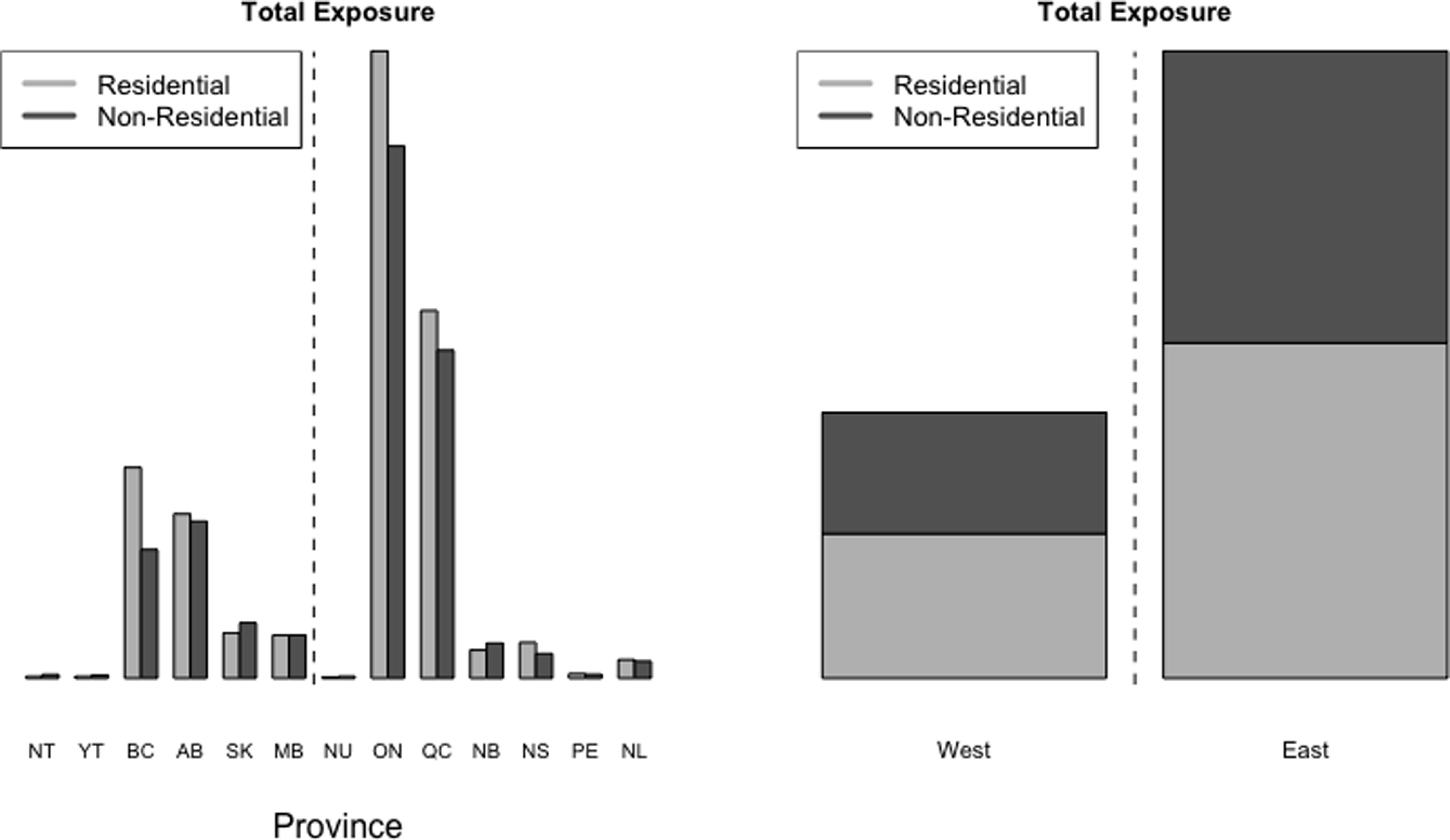


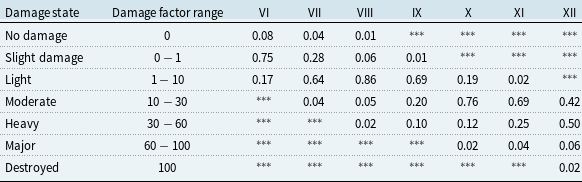


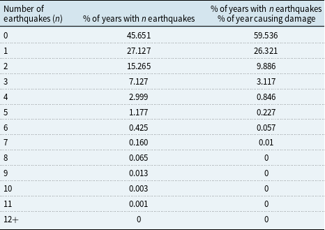


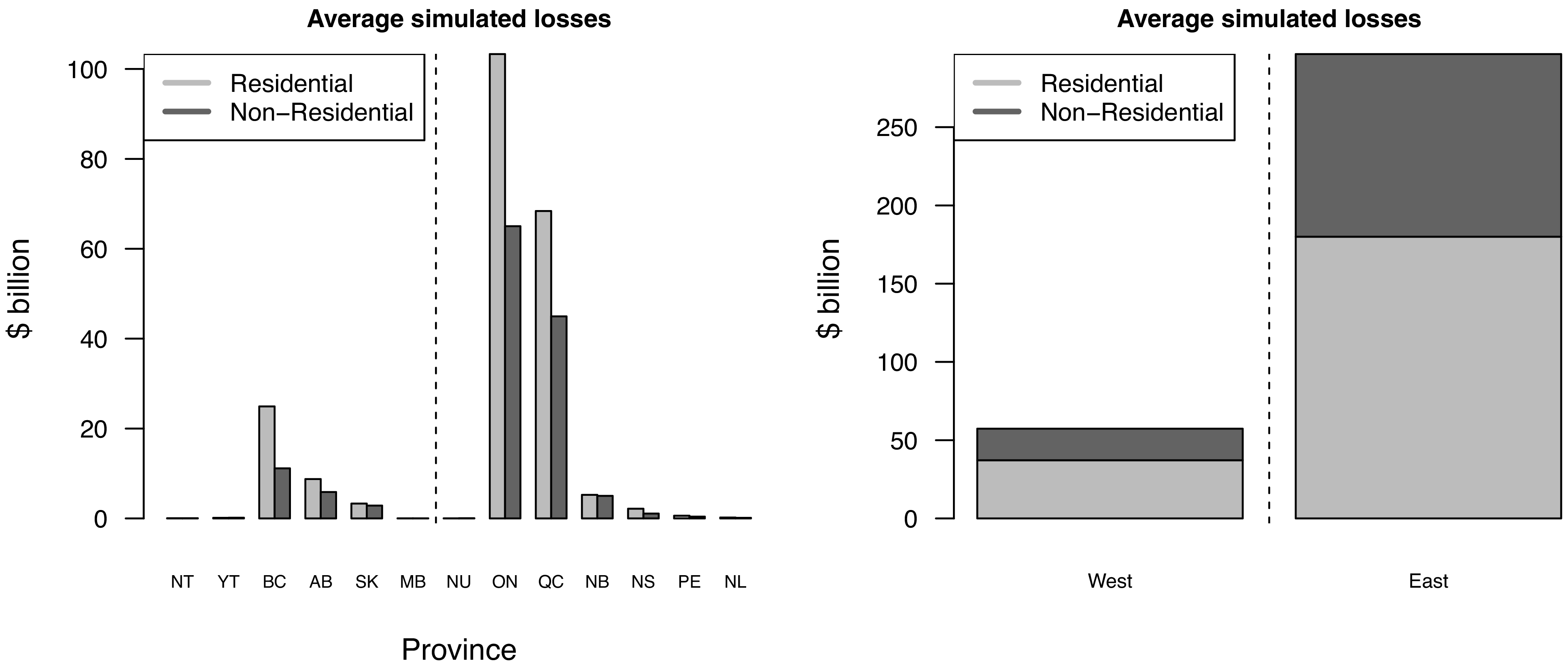
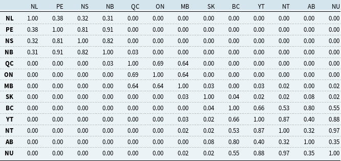
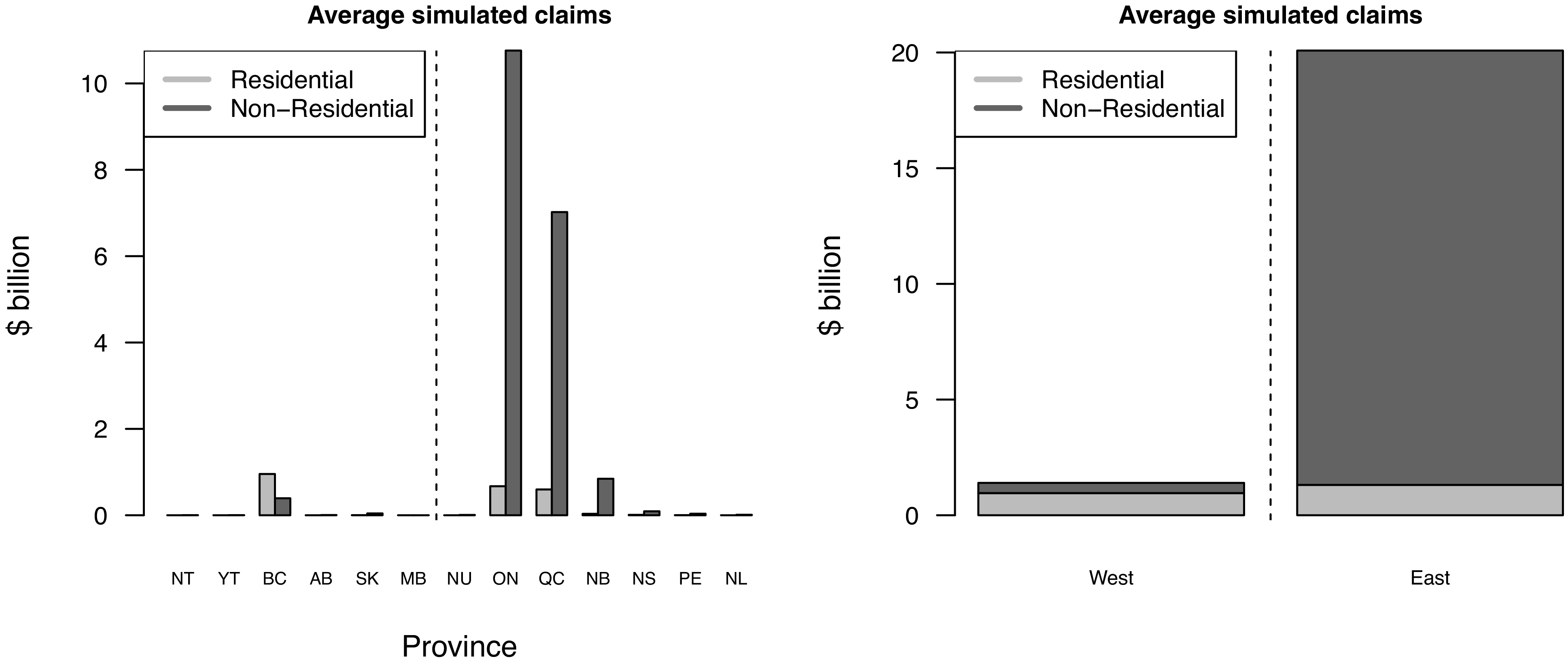
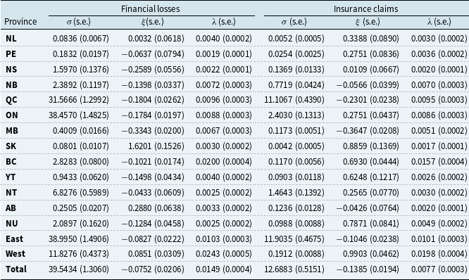
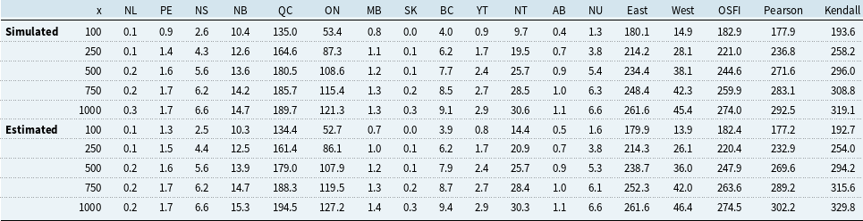


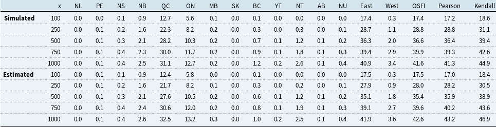


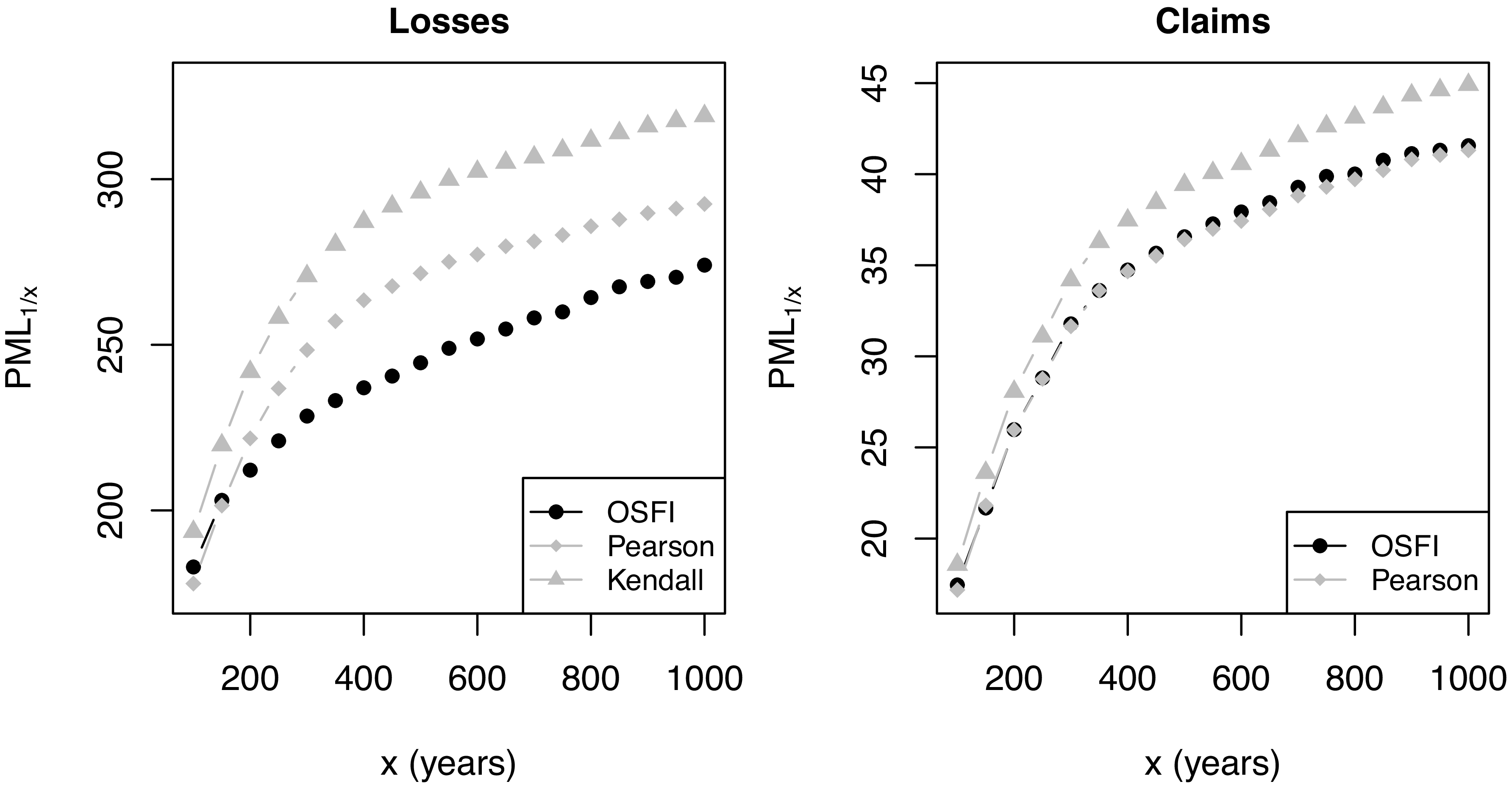


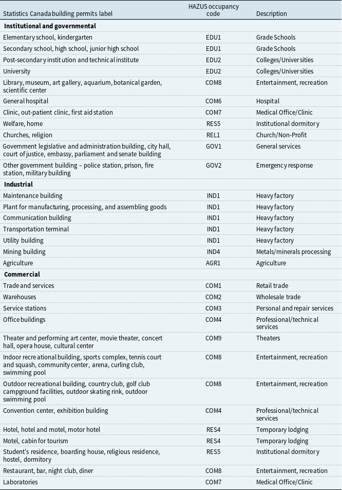


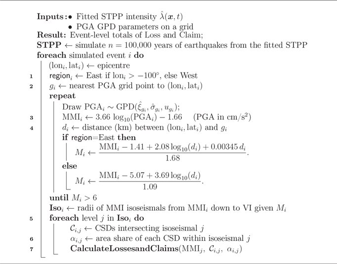
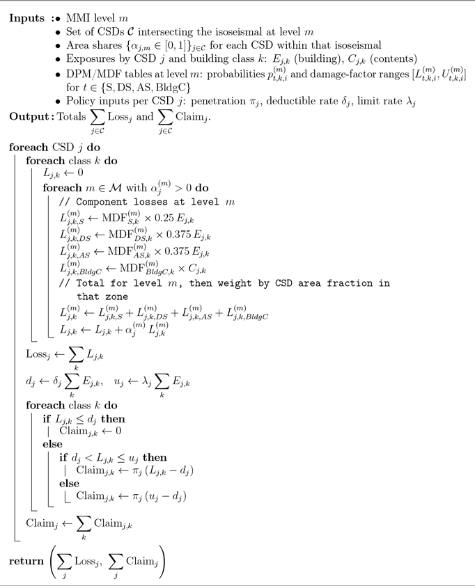
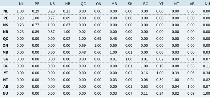
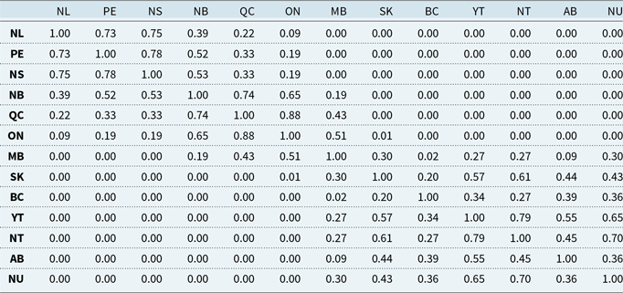
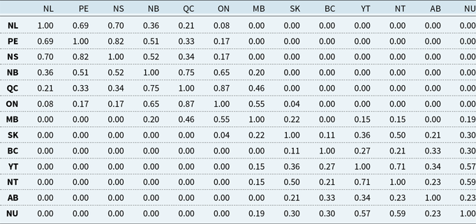


 Open access