


1 Introduction
1.1 Motivation
The Bruggeman-Kuznetsov formula, one of the core tools of analytic number theory since the late 1970s, can be stated in its simplest form as follows. Given a test function
 $h_\infty (t)$
one defines the Kuznetsov transform of it by
$h_\infty (t)$
one defines the Kuznetsov transform of it by
 $$ \begin{align} H_\infty(x) = \frac{i}{2} \int_{-\infty}^\infty \frac{J_{2it}(x)}{\cosh (\pi t)} h_\infty(t) t\,dt. \end{align} $$
For sufficiently well-behaved test functions
 $h_\infty $
(see (1.5)) and integers
$h_\infty $
(see (1.5)) and integers
 $m,n$
with
$m,n$
with
 $mn>0$
one has
$mn>0$
one has
 $$ \begin{align} \sum_{u \in \mathcal{B}_0} h_\infty(t_u) a_u(m)&\overline{a_u(n)}+ \frac{1}{4\pi} \int_{-\infty}^\infty h_\infty(t) \frac{\pi}{|\zeta(1+2it)|^2} \lambda_t(m) \overline{\lambda_t(n)}\,dt \\ & = \delta_{m=n} \frac{1}{4\pi} \int_{-\infty}^{\infty} h_{\infty}(t) t \tanh(\pi t) dt + \sum_{c \in \mathbb{N}} \frac{S(m,n;c)}{c} H_{\infty}\Big(\frac{4 \pi \sqrt{|mn|}}{c}\Big) \nonumber \end{align} $$
where
 $\mathcal {B}_0$
is an orthonormal basis of Hecke-Maass waveforms u on
$\mathcal {B}_0$
is an orthonormal basis of Hecke-Maass waveforms u on
 $\operatorname {\mathrm {SL}}_2(\mathbb {Z}) \backslash \mathcal {H}$
normalized by
$\operatorname {\mathrm {SL}}_2(\mathbb {Z}) \backslash \mathcal {H}$
normalized by
 $\operatorname {\mathrm {vol}}( \operatorname {\mathrm {SL}}_2(\mathbb {Z}) \backslash \mathcal {H})=\pi /3$
,
$\operatorname {\mathrm {vol}}( \operatorname {\mathrm {SL}}_2(\mathbb {Z}) \backslash \mathcal {H})=\pi /3$
,
 $1/4 + t_u^{2}$
is the Laplace eigenvalue of u,
$1/4 + t_u^{2}$
is the Laplace eigenvalue of u,
 $a_u(m)$
are the Fourier coefficients given by
$a_u(m)$
are the Fourier coefficients given by
 $$ \begin{align*}u(x+iy) = 2 \sqrt{y} \left( \frac{\cosh (\pi t_u)}{\pi}\right)^{1/2} \sum_{n \neq 0} a_u(n) K_{it_u}(2 \pi |n| y)e(nx),\end{align*} $$
the
 $\lambda _t(n) = \sum _{ab=|n|}(b/a)^{it}$
, and
$\lambda _t(n) = \sum _{ab=|n|}(b/a)^{it}$
, and
 $$ \begin{align*}S(m,n;c)= \sideset{}{^*}\sum_{x\ \pmod{c}} e\left(\frac{mx + n \overline{x}}{c}\right)\end{align*} $$
is the Kloosterman sum, in which the
 $*$
indicates that the sum runs over invertible residue classes modulo c and
$*$
indicates that the sum runs over invertible residue classes modulo c and
 $\overline {x}$
denotes the inverse of x modulo c. There is also an opposite-sign version of (1.2) that holds in the case
$\overline {x}$
denotes the inverse of x modulo c. There is also an opposite-sign version of (1.2) that holds in the case
 $mn<0$
with the modification that
$mn<0$
with the modification that
 $H_\infty (x)$
is replaced by a function
$H_\infty (x)$
is replaced by a function
 $H_\infty ^-(x)$
(see (1.23)).
$H_\infty ^-(x)$
(see (1.23)).
Even more classical is the holomorphic counterpart to (1.2), i.e. the Petersson formula:
 $$ \begin{align} \sum_{f \in \mathcal{B}_\kappa} a_{f}(m) \overline{a_{f}(n)} = \frac{\kappa-1}{4\pi} \left(\delta_{m=n} + 2 \pi i^{-\kappa} \sum_{c\in \mathbb{N}} \frac{S(m,n;c)}{c} J_{\kappa -1}\Big(\frac{4 \pi \sqrt{mn}}{c}\Big)\right), \end{align} $$
where
 $\mathcal {B}_\kappa $
is an orthonormal basis of holomorphic cusp forms f for
$\mathcal {B}_\kappa $
is an orthonormal basis of holomorphic cusp forms f for
 $\operatorname {\mathrm {SL}}_2(\mathbb {Z})$
of weight
$\operatorname {\mathrm {SL}}_2(\mathbb {Z})$
of weight
 $\kappa $
and Fourier coefficients
$\kappa $
and Fourier coefficients
 $a_f(m)$
given by
$a_f(m)$
given by
 $$ \begin{align*}f(z) = \left( \frac{(4\pi)^\kappa}{\Gamma(\kappa)}\right)^{1/2} \sum_{n\geq 1} a_f(n) n^{\frac{\kappa-1}{2}}e(nz).\end{align*} $$
In the representation-theoretic framework for automorphic forms, the parity
 $p(u)$
(see (1.22)) and spectral parameter
$p(u)$
(see (1.22)) and spectral parameter
 $t_u$
or weight
$t_u$
or weight
 $\kappa =\kappa _f$
parametrize the possible archimedean local components
$\kappa =\kappa _f$
parametrize the possible archimedean local components
 $\pi _\infty $
of trivial central character cuspidal automorphic representations
$\pi _\infty $
of trivial central character cuspidal automorphic representations
 $\pi $
of
$\pi $
of
 $\operatorname {\mathrm {GL}}_2/\mathbb Q$
. Therefore, the above Bruggeman-Kuznetsov (both
$\operatorname {\mathrm {GL}}_2/\mathbb Q$
. Therefore, the above Bruggeman-Kuznetsov (both
 $mn>0$
and
$mn>0$
and
 $mn<0$
cases) and Petersson formulas can be combined to give a spectral summation device for automorphic forms on
$mn<0$
cases) and Petersson formulas can be combined to give a spectral summation device for automorphic forms on
 $\operatorname {\mathrm {PGL}}_2/\mathbb Q$
with specified local representation at infinity (and that are unramified at all finite places).
$\operatorname {\mathrm {PGL}}_2/\mathbb Q$
with specified local representation at infinity (and that are unramified at all finite places).
The goal of this paper is to analogously develop Petersson/Bruggeman-Kuznetsov (PBK) formulas at finite places p that allow control on the associated representations of
 $\operatorname {\mathrm {GL}}_2(\mathbb Q_p)$
at those places (as well as at
$\operatorname {\mathrm {GL}}_2(\mathbb Q_p)$
at those places (as well as at
 $\infty $
). To generate such formulas, we use the adelic relative trace formula approach to the PBK formulas of Jacquet [Reference JacquetJac86] and Zagier [Reference ZagierZag81, Reference JoynerJoy90], as exposited by Knightly and Li [Reference Knightly and LiKL06a, Reference Knightly and LiKL13]. We restrict our attention to automorphic forms over
$\infty $
). To generate such formulas, we use the adelic relative trace formula approach to the PBK formulas of Jacquet [Reference JacquetJac86] and Zagier [Reference ZagierZag81, Reference JoynerJoy90], as exposited by Knightly and Li [Reference Knightly and LiKL06a, Reference Knightly and LiKL13]. We restrict our attention to automorphic forms over
 $\mathbb Q$
in this paper, but many of the local aspects of our work should carry over to more general non-archimedean local fields.
$\mathbb Q$
in this paper, but many of the local aspects of our work should carry over to more general non-archimedean local fields.
In this perspective, one chooses a test function f on the group
 $\operatorname {\mathrm {GL}}_2(\mathbb {A})$
for the pretrace formula and then integrates along left and right unipotent orbits to obtain the PBK formula. To aid this strategy and to produce a reasonably explicit formula, we introduce two assumptions on the test function f called the geometric and spectral assumptions. The geometric assumptions place a constraint on the support of the local test function
$\operatorname {\mathrm {GL}}_2(\mathbb {A})$
for the pretrace formula and then integrates along left and right unipotent orbits to obtain the PBK formula. To aid this strategy and to produce a reasonably explicit formula, we introduce two assumptions on the test function f called the geometric and spectral assumptions. The geometric assumptions place a constraint on the support of the local test function
 $f_p$
on
$f_p$
on
 $\operatorname {\mathrm {GL}}_2(\mathbb Q_p)$
and allow us to establish the standard properties of the geometric side of the formula. The spectral assumption puts a strong constraint on the integral operators
$\operatorname {\mathrm {GL}}_2(\mathbb Q_p)$
and allow us to establish the standard properties of the geometric side of the formula. The spectral assumption puts a strong constraint on the integral operators
 $\pi (f)$
and allows us to explicate the spectral side of the formula. The result is Theorem 1.8.
$\pi (f)$
and allows us to explicate the spectral side of the formula. The result is Theorem 1.8.
As an application of Theorem 1.8, we give a harmonically weighted Weyl-Selberg Law for the family of cusp forms
 $\mathcal {F}_0(f)$
cut out by our chosen test function f and interpret the leading constant in terms of local Plancherel volumes. For this result, see Corollary 1.14. In a similar context, Palm [Reference PalmPal12, Thm. 3.2.1] gave a Weyl law for cusp forms with specified local components as an application of the Selberg trace formula.
$\mathcal {F}_0(f)$
cut out by our chosen test function f and interpret the leading constant in terms of local Plancherel volumes. For this result, see Corollary 1.14. In a similar context, Palm [Reference PalmPal12, Thm. 3.2.1] gave a Weyl law for cusp forms with specified local components as an application of the Selberg trace formula.
As a second application of Theorem 1.8, we give an axiomatized Large Sieve Inequality for the families
 $\mathcal {F}_0(f)$
cut out by f. Under additional local hypotheses (stated in Section 1.5) these large sieve inequalities are optimally strong: the estimate is of the shape
$\mathcal {F}_0(f)$
cut out by f. Under additional local hypotheses (stated in Section 1.5) these large sieve inequalities are optimally strong: the estimate is of the shape
 $\ll (X|\mathcal {F}|)^\varepsilon (X + |\mathcal {F}|)\|\mathbf {a}\|_2^2$
, where X is the length of summation of the sequence
$\ll (X|\mathcal {F}|)^\varepsilon (X + |\mathcal {F}|)\|\mathbf {a}\|_2^2$
, where X is the length of summation of the sequence
 $\mathbf {a}$
and
$\mathbf {a}$
and
 $|\mathcal {F}|$
is the cardinality of the family of cusp forms.
$|\mathcal {F}|$
is the cardinality of the family of cusp forms.
Probably the most important part of the paper however are the examples. Most notably, in Section 6.4 we give an elegant expression for the generalized Kloosterman sum that arises from a specified (trivial central character) supercuspidal representation
 $\sigma $
of
$\sigma $
of
 $\operatorname {\mathrm {GL}}_2(\mathbb Q_p)$
. See Theorem 6.45 for this formula.
$\operatorname {\mathrm {GL}}_2(\mathbb Q_p)$
. See Theorem 6.45 for this formula.
For the specified supercuspidal formula, we set the local test function
 $f_p$
equal to the diagonal newform matrix coefficient of
$f_p$
equal to the diagonal newform matrix coefficient of
 $\sigma $
restricted to a maximal compact subgroup, building on earlier work of the first author [Reference HuHu24]. This test function
$\sigma $
restricted to a maximal compact subgroup, building on earlier work of the first author [Reference HuHu24]. This test function
 $f_p$
generates a generalized PBK formula that selects on the spectral side automorphic forms with local component at p isomorphic to either
$f_p$
generates a generalized PBK formula that selects on the spectral side automorphic forms with local component at p isomorphic to either
 $\sigma $
or at most two other supercuspidal representations of the same conductor. This is essentially the narrowest possible support on the spectral side under the geometric assumptions. For precise statements, see Theorems 6.20 and 6.29.
$\sigma $
or at most two other supercuspidal representations of the same conductor. This is essentially the narrowest possible support on the spectral side under the geometric assumptions. For precise statements, see Theorems 6.20 and 6.29.
In a parallel fashion, given a primitive Dirichlet character
 $\chi $
modulo a power of p with
$\chi $
modulo a power of p with
 $\chi ^2 \neq 1$
, we construct local test functions
$\chi ^2 \neq 1$
, we construct local test functions
 $f_\chi $
in Section 7.2 whose generalized PBK formula selects on the spectral side automorphic forms with local component at p isomorphic to a principal series representations
$f_\chi $
in Section 7.2 whose generalized PBK formula selects on the spectral side automorphic forms with local component at p isomorphic to a principal series representations
 $\pi (\chi |\cdot |_p^{it} ,\chi ^{-1}|\cdot |_p^{-it})$
for some
$\pi (\chi |\cdot |_p^{it} ,\chi ^{-1}|\cdot |_p^{-it})$
for some
 $t\in \mathbb R$
. The generalized Kloosterman sum on the geometric side of the formula (7.16) is in complete analogy with the supercuspidal Kloosterman sum mentioned above. Again, this generalized PBK formula has the narrowest possible support on the spectral side under the geometric assumptions (see Lemma 3.11).
$t\in \mathbb R$
. The generalized Kloosterman sum on the geometric side of the formula (7.16) is in complete analogy with the supercuspidal Kloosterman sum mentioned above. Again, this generalized PBK formula has the narrowest possible support on the spectral side under the geometric assumptions (see Lemma 3.11).
These examples lay the groundwork for future important analytic applications. That we can produce several interesting examples that satisfy both the geometric and spectral hypotheses shows that while these two hypotheses together may appear fairly restrictive, they nonetheless contain the families of greatest interest to us.
An important feature of the Bruggeman-Kuznetsov (BK) formula is that the integral transform (1.1) relating the test function
 $h_\infty $
on the spectral side to the archimedean test function
$h_\infty $
on the spectral side to the archimedean test function
 $H_\infty $
on the geometric side is relatively simple and can often be analyzed effectively using standard techniques such as stationary phase estimates. The situation (at present) with finite places is not quite as clean: the local test function
$H_\infty $
on the geometric side is relatively simple and can often be analyzed effectively using standard techniques such as stationary phase estimates. The situation (at present) with finite places is not quite as clean: the local test function
 $f_p$
on
$f_p$
on
 $\operatorname {\mathrm {GL}}_2(\mathbb Q_p)$
continues to play a strong role in the formula whereas the test function
$\operatorname {\mathrm {GL}}_2(\mathbb Q_p)$
continues to play a strong role in the formula whereas the test function
 $f_\infty $
on
$f_\infty $
on
 $\operatorname {\mathrm {GL}}_2(\mathbb R)$
can be completely suppressed from the classical BK formula.
$\operatorname {\mathrm {GL}}_2(\mathbb R)$
can be completely suppressed from the classical BK formula.
Nonetheless, we develop the sequence of transforms
 $$ \begin{align*}h_p \to f_p \to H_p\end{align*} $$
to some extent, where
 $h_p: \pi \mapsto \pi (f_p)$
is an operator-valued function on the unitary dual of
$h_p: \pi \mapsto \pi (f_p)$
is an operator-valued function on the unitary dual of
 $\operatorname {\mathrm {PGL}}_2(\mathbb Q_p)$
(assumed to be projections with finite-dimensional image) and
$\operatorname {\mathrm {PGL}}_2(\mathbb Q_p)$
(assumed to be projections with finite-dimensional image) and
 $H_p$
are the generalized (local) Kloosterman sums defined in (3.13). Indeed, Proposition 4.1 gives an expression for
$H_p$
are the generalized (local) Kloosterman sums defined in (3.13). Indeed, Proposition 4.1 gives an expression for
 $f_p$
as an integral transform (of sorts) of
$f_p$
as an integral transform (of sorts) of
 $h_p$
in terms of matrix coefficients over the unitary dual
$h_p$
in terms of matrix coefficients over the unitary dual
 $\operatorname {\mathrm {PGL}}_2(\mathbb Q_p)$
with respect to Plancherel measure. Then
$\operatorname {\mathrm {PGL}}_2(\mathbb Q_p)$
with respect to Plancherel measure. Then
 $H_p$
is by definition an integral of
$H_p$
is by definition an integral of
 $f_p$
against additive characters. Furthermore, Section 7 gives a list of transform pairs
$f_p$
against additive characters. Furthermore, Section 7 gives a list of transform pairs
 $h_p \to H_p$
for which one can mostly forget about the function
$h_p \to H_p$
for which one can mostly forget about the function
 $f_p$
on the group entirely.
$f_p$
on the group entirely.
As already mentioned, much of this paper builds on previous work of the first author [Reference HuHu24]. To be definite, our paper contains the following new features:
-
• an axiomatized treatment of PBK formulas given by adelic test functions (see the geometric and spectral assumptions in Section 1.2),
-
• some preliminary applications of the axiomatized PBK formulas (see Section 5),
-
• a test function with smallest possible spectral support around a specified supercuspidal representation
 $\sigma $
with even conductor exponent, i.e. we achieve
$l_0=0$
in the sense of [Reference HuHu24, Rem. 1.4], see the discussion around Theorem 6.20 in this paper,
$\sigma $
with even conductor exponent, i.e. we achieve
$l_0=0$
in the sense of [Reference HuHu24, Rem. 1.4], see the discussion around Theorem 6.20 in this paper, -
• a more natural expression for the generalized Kloosterman sum associated to a specified supercuspidal representation (compare [Reference HuHu24, Def. 4.6] and Theorem 6.45), and
-
• a detailed treatment of the dihedral
$p=2$
case, which is often omitted for convenience but hides many technical complications (see Section 6.3).


1.2 Statement of results
Let
 $G=\operatorname {\mathrm {GL}}_2$
and
$G=\operatorname {\mathrm {GL}}_2$
and
 $\overline {G} =\operatorname {\mathrm {PGL}}_2$
. Write
$\overline {G} =\operatorname {\mathrm {PGL}}_2$
. Write
 ${\mathcal {H}}_{\mathrm {fin}} =C_c^\infty (\overline {G}(\mathbb {A}_{\mathrm {fin}}))$
for the non-archimedean Hecke algebra of
${\mathcal {H}}_{\mathrm {fin}} =C_c^\infty (\overline {G}(\mathbb {A}_{\mathrm {fin}}))$
for the non-archimedean Hecke algebra of
 $\overline {G}$
, that is the space of locally constant functions on
$\overline {G}$
, that is the space of locally constant functions on
 $G(\mathbb {A}_{\mathrm {fin}})$
that are invariant by and compactly supported modulo center
$G(\mathbb {A}_{\mathrm {fin}})$
that are invariant by and compactly supported modulo center
 $Z(\mathbb {A}_{\mathrm {fin}})$
. Define the local Hecke algebra
$Z(\mathbb {A}_{\mathrm {fin}})$
. Define the local Hecke algebra
 ${\mathcal {H}}_p= C_c^\infty (\overline {G}(\mathbb Q_p))$
similarly.
${\mathcal {H}}_p= C_c^\infty (\overline {G}(\mathbb Q_p))$
similarly.
Let
 $K_p = G(\mathbb {Z}_p)$
and
$K_p = G(\mathbb {Z}_p)$
and
 $ZK_p = Z(\mathbb Q_p)G(\mathbb {Z}_p)$
for
$ZK_p = Z(\mathbb Q_p)G(\mathbb {Z}_p)$
for
 $p<\infty $
. We say that a pure tensor
$p<\infty $
. We say that a pure tensor
 $f= \bigotimes _p f_p \in {\mathcal {H}}_{\mathrm {fin}}$
is ramified at a prime p if
$f= \bigotimes _p f_p \in {\mathcal {H}}_{\mathrm {fin}}$
is ramified at a prime p if
 $f_p$
is not a constant multiple of
$f_p$
is not a constant multiple of
 $1_{ZK_p}$
. Let
$1_{ZK_p}$
. Let
 $K = \prod _p K_p$
be the standard maximal compact subgroup of
$K = \prod _p K_p$
be the standard maximal compact subgroup of
 $G(\mathbb {A}_{\mathrm {fin}})$
and let
$G(\mathbb {A}_{\mathrm {fin}})$
and let
 $K(N)$
be the principal congruence subgroup of K. The minimal
$K(N)$
be the principal congruence subgroup of K. The minimal
 $N \in \mathbb {N}$
such that
$N \in \mathbb {N}$
such that
 $f \in {\mathcal {H}}_{\mathrm {fin}}$
is bi-
$f \in {\mathcal {H}}_{\mathrm {fin}}$
is bi-
 $K(N)$
-invariant is called the level of f.
$K(N)$
-invariant is called the level of f.
Our generalized Bruggeman-Kuznetsov formula is an equality between a spectral sum of Fourier coefficients/Hecke eigenvalues over a family of automorphic forms and a geometric sum of generalized Kloosterman sums over a set of admissible moduli. In the next several paragraphs, we define these objects.
For an irreducible admissible representation
 $(\pi , V_\pi )$
with
$(\pi , V_\pi )$
with
 $\pi _{\mathrm {fin}}$
the underlying
$\pi _{\mathrm {fin}}$
the underlying
 $\overline {G}(\mathbb {A}_{\mathrm {fin}})$
-representation and
$\overline {G}(\mathbb {A}_{\mathrm {fin}})$
-representation and
 $f\in {\mathcal {H}}_{\mathrm {fin}}$
, we write
$f\in {\mathcal {H}}_{\mathrm {fin}}$
, we write
 $\pi (f): V_{\pi } \to V_{\pi }$
for the integral operator
$\pi (f): V_{\pi } \to V_{\pi }$
for the integral operator
 $$ \begin{align} \pi(f): v \mapsto \int_{\overline{G}(\mathbb{A}_{\mathrm{fin}})} f(g) \pi_{\mathrm{fin}}(g)v\,dg. \end{align} $$
Note that
 $\pi (f):=\pi _{\mathrm {fin}}(f)$
but we have dropped the subscript to avoid cluttering the notation.
$\pi (f):=\pi _{\mathrm {fin}}(f)$
but we have dropped the subscript to avoid cluttering the notation.
Definition 1.1 (Family cut out by f).
We write
 $\mathcal {F}_0(f)$
for the set of cuspidal automorphic representations
$\mathcal {F}_0(f)$
for the set of cuspidal automorphic representations
 $\pi $
that are spherical at
$\pi $
that are spherical at
 $\infty $
and such that
$\infty $
and such that
 $\pi (f): V_{\pi } \to V_{\pi }$
is not the zero map.
$\pi (f): V_{\pi } \to V_{\pi }$
is not the zero map.
The family
 $\mathcal {F}_0(f)$
has no restrictions on the archimedean spectral parameters of the representation it contains. Such restrictions will be imposed in our formulas in the standard way: by selecting a test function
$\mathcal {F}_0(f)$
has no restrictions on the archimedean spectral parameters of the representation it contains. Such restrictions will be imposed in our formulas in the standard way: by selecting a test function
 $h_\infty $
. Note that
$h_\infty $
. Note that
 $\mathcal {F}_0(f)$
is a harmonic family in the sense of [Reference Sarnak, Shin and TemplierSST16], and at least in spirit every harmonic family on
$\mathcal {F}_0(f)$
is a harmonic family in the sense of [Reference Sarnak, Shin and TemplierSST16], and at least in spirit every harmonic family on
 $\operatorname {\mathrm {PGL}}_2$
over
$\operatorname {\mathrm {PGL}}_2$
over
 $\mathbb Q$
arises in this way.
$\mathbb Q$
arises in this way.
For
 $\pi $
a cuspidal automorphic representation, write
$\pi $
a cuspidal automorphic representation, write
 $\mathcal {B}(\pi )$
for an orthonormal basis of
$\mathcal {B}(\pi )$
for an orthonormal basis of
 $V_\pi $
(with respect to (1.61)). Let
$V_\pi $
(with respect to (1.61)). Let
 $K_\infty = \operatorname {\mathrm {SO}}_2(\mathbb R)$
. The subspace
$K_\infty = \operatorname {\mathrm {SO}}_2(\mathbb R)$
. The subspace
 $V_\pi ^{K_\infty \times K(N)}$
of fixed vectors in
$V_\pi ^{K_\infty \times K(N)}$
of fixed vectors in
 $\pi $
is finite-dimensional, and for cuspidal
$\pi $
is finite-dimensional, and for cuspidal
 $\pi $
let
$\pi $
let
 $u=u_\varphi $
be the classical Maass waveform with respect to
$u=u_\varphi $
be the classical Maass waveform with respect to
 $\Gamma (N)$
corresponding to
$\Gamma (N)$
corresponding to
 $\varphi \in V_\pi ^{K_\infty \times K(N)}$
by
$\varphi \in V_\pi ^{K_\infty \times K(N)}$
by
 $u(x+iy) = \varphi ( \left ( \begin {smallmatrix} y & x \\ & 1\end {smallmatrix}\right ) \times 1_{\mathrm {fin}}).$
Recall from (2.9) the Fourier coefficients
$u(x+iy) = \varphi ( \left ( \begin {smallmatrix} y & x \\ & 1\end {smallmatrix}\right ) \times 1_{\mathrm {fin}}).$
Recall from (2.9) the Fourier coefficients
 $a_u(m)$
for
$a_u(m)$
for
 $m\in \frac {1}{N}\mathbb {Z}$
of a Maass form u for
$m\in \frac {1}{N}\mathbb {Z}$
of a Maass form u for
 $\Gamma (N)$
.
$\Gamma (N)$
.
Let
 $h_\infty (t)$
be a test function as in the classical Kuznetsov formula. Iwaniec and Kowalski [Reference Iwaniec and KowalskiIK04, (15.19)] give the following sufficient conditions: For some
$h_\infty (t)$
be a test function as in the classical Kuznetsov formula. Iwaniec and Kowalski [Reference Iwaniec and KowalskiIK04, (15.19)] give the following sufficient conditions: For some
 $\delta>0$
 $$ \begin{align} \begin{cases} h_\infty(t) \text{ is holomorphic in } |\mathrm{Im}(t)| \leq 1/2+\delta, \\ h_{\infty}(t)\ll (1+|t|)^{-2-\delta}, \text{ and } \\ h_\infty(t)= h_\infty(-t) \text{ for all } t. \end{cases} \end{align} $$
Let
 $\psi _p: \mathbb Q_p\to \mathbb {C}^\times $
be the standard additive character
$\psi _p: \mathbb Q_p\to \mathbb {C}^\times $
be the standard additive character
 $\psi _p(x)= e(\{x\}_p)$
and
$\psi _p(x)= e(\{x\}_p)$
and
 $\psi _{\mathrm {fin}} : \mathbb {A}_{\mathrm {fin}} \to \mathbb {C}^\times $
be given by
$\psi _{\mathrm {fin}} : \mathbb {A}_{\mathrm {fin}} \to \mathbb {C}^\times $
be given by
 $\psi _{\mathrm {fin}} = \prod _p \psi _p$
.
$\psi _{\mathrm {fin}} = \prod _p \psi _p$
.
Definition 1.2. For
 $f \in {\mathcal {H}}_{\mathrm {fin}}$
,
$f \in {\mathcal {H}}_{\mathrm {fin}}$
,
 $m,n \in \mathbb Q$
and
$m,n \in \mathbb Q$
and
 $c \in \mathbb Q_+$
, the generalized Kloosterman sum (attached to f) that appears in this paper is defined as
$c \in \mathbb Q_+$
, the generalized Kloosterman sum (attached to f) that appears in this paper is defined as
 $$ \begin{align} H(m_1,m_2;c) = \iint_{\mathbb{A}_{\mathrm{fin}}^2} f\left( \left( \begin{smallmatrix}1 & -t_1 \\ & 1 \end{smallmatrix}\right) \left( \begin{smallmatrix} & -c^{-2} \\ 1 & \end{smallmatrix}\right) \left( \begin{smallmatrix}1 & t_2 \\ & 1 \end{smallmatrix}\right) \right) \psi_{\mathrm{fin}}(m_1t_1- m_2 t_2)\,dt_1\,dt_2. \end{align} $$
Note that
 $H(m_1, m_2;c)$
is in fact a finite sum since
$H(m_1, m_2;c)$
is in fact a finite sum since
 $f\in {\mathcal {H}}_{\mathrm {fin}}$
. While the sum
$f\in {\mathcal {H}}_{\mathrm {fin}}$
. While the sum
 $H(m,n;c)$
is à priori defined for all
$H(m,n;c)$
is à priori defined for all
 $m,n \in \mathbb Q$
, it vanishes unless
$m,n \in \mathbb Q$
, it vanishes unless
 $m,n \in \frac {1}{N}\mathbb {Z}$
(see Theorem 3.8(1)). We also define local generalized Kloosterman sums
$m,n \in \frac {1}{N}\mathbb {Z}$
(see Theorem 3.8(1)). We also define local generalized Kloosterman sums
 $H_p(m,n;c)$
by the same formula (1.6) but where
$H_p(m,n;c)$
by the same formula (1.6) but where
 $\mathbb {A}_{\mathrm {fin}}, \psi _{\mathrm {fin}},$
and f are replaced by their local versions
$\mathbb {A}_{\mathrm {fin}}, \psi _{\mathrm {fin}},$
and f are replaced by their local versions
 $\mathbb Q_p, \psi _p,$
and
$\mathbb Q_p, \psi _p,$
and
 $f_p$
(to be definite, see (3.13)).
$f_p$
(to be definite, see (3.13)).
When
 $f=\bigotimes _p f_p$
is a pure tensor, one has
$f=\bigotimes _p f_p$
is a pure tensor, one has
 $H(m,n;c) = \prod _p H_p(m,n;c)$
. Of course the generalized Kloosterman sum
$H(m,n;c) = \prod _p H_p(m,n;c)$
. Of course the generalized Kloosterman sum
 $H(m,n;c)$
depends on
$H(m,n;c)$
depends on
 $f \in {\mathcal {H}}_{\mathrm {fin}}$
and the local
$f \in {\mathcal {H}}_{\mathrm {fin}}$
and the local
 $H_p(m,n;c)$
depend on
$H_p(m,n;c)$
depend on
 $f_p\in {\mathcal {H}}_p$
, but these are suppressed in the notation. Recall, we also defined the transform
$f_p\in {\mathcal {H}}_p$
, but these are suppressed in the notation. Recall, we also defined the transform
 $H_\infty (x)$
of
$H_\infty (x)$
of
 $h_\infty (t)$
by (1.1), as in the classical Kuznetsov formula.
$h_\infty (t)$
by (1.1), as in the classical Kuznetsov formula.
Next we define the index set of the sum on the geometric side of our formula.
Proposition/Definition 1.3 (Admissible moduli).
We say
 $c \in \mathbb Q_+$
is an admissible modulus if there exists a pair
$c \in \mathbb Q_+$
is an admissible modulus if there exists a pair
 $(m,n)\in \mathbb Q^2$
so that
$(m,n)\in \mathbb Q^2$
so that
 $H(m,n;c)\neq 0,$
and write
$H(m,n;c)\neq 0,$
and write
 $\mathcal {C}(\mathcal {F})\subseteq \mathbb Q_+$
for the set of admissible moduli. If
$\mathcal {C}(\mathcal {F})\subseteq \mathbb Q_+$
for the set of admissible moduli. If
 $f = \bigotimes _p f_p \in {\mathcal {H}}_{\mathrm {fin}}$
is a pure tensor and
$f = \bigotimes _p f_p \in {\mathcal {H}}_{\mathrm {fin}}$
is a pure tensor and
 $\operatorname {\mathrm {supp}} f_p$
is contained in
$\operatorname {\mathrm {supp}} f_p$
is contained in
 $\{g \in G(\mathbb Q_p): \det g \in \mathbb {Z}_p^\times (\mathbb Q_p^\times )^2\}$
for all p, then there exists
$\{g \in G(\mathbb Q_p): \det g \in \mathbb {Z}_p^\times (\mathbb Q_p^\times )^2\}$
for all p, then there exists
 $q' \in \mathbb Q_+$
such that
$q' \in \mathbb Q_+$
such that
 $\mathcal {C}(\mathcal {F}) \subseteq q'\mathbb {Z}$
.
$\mathcal {C}(\mathcal {F}) \subseteq q'\mathbb {Z}$
.
See Lemma 2.5 for a proof. Under the mild hypothesis in the second sentence of Proposition/Definition 1.3, it is not too hard to show that one has an “unrefined” Bruggeman-Kuznetsov formula of the shape
 $$ \begin{align} \sum_{ \pi \in \mathcal{F}_0(f)} h_\infty(t_\pi) & \sum_{\varphi \in \mathcal{B}(\pi)}a_{u_{\pi(f)\varphi}}(m_1) \overline{a_{u_\varphi}(m_2) } + (\text{cts.}) \\ & = (\text{diag.\ weight})\delta_{m_1=m_2} + \sum_{c \in \mathcal{C}(\mathcal{F}) } \frac{H(m_1,m_2;c)}{c}H_\infty\left(\frac{4 \pi \sqrt{ m_1m_2}}{c}\right).\nonumber \end{align} $$
For more details, see Theorem 2.1. On its own, (1.7) is not very useful without additional information on f.
We next introduce the geometric and spectral assumptions alluded to in Section 1.1, which permit a practically useful refinement of (1.7). Let
 $a(y)= \left (\begin {smallmatrix} y & 0 \\ 0 & 1 \end {smallmatrix}\right )$
and
$a(y)= \left (\begin {smallmatrix} y & 0 \\ 0 & 1 \end {smallmatrix}\right )$
and
 $A\subset G$
be as in Section 1.7.3.
$A\subset G$
be as in Section 1.7.3.
Geometric Assumptions.
-
(1) The function
$f \in {\mathcal {H}}_{\mathrm {fin}}$
is bi-
$A(\widehat {\mathbb {Z}})$
-invariant. -
(2) There exists
$y\in \mathbb Q_+$
such that
$\operatorname {\mathrm {supp}} f \subseteq a(y)^{-1}ZK a(y)$
.


We say that a rational number
 $y \in \mathbb Q_+$
for which Geometric Assumption (2) holds “controls the support of f”. Caution: y is not necessarily uniquely determined by f. Note, Geometric Assumption (2) ensures that the hypothesis on the support of f of Theorem 2.1 is satisfied. Another useful fact to keep in mind is that under Geometric Assumption (2), the function f is ramified at p if and only if p divides the level of f, for which see Section 1.3.1.
$y \in \mathbb Q_+$
for which Geometric Assumption (2) holds “controls the support of f”. Caution: y is not necessarily uniquely determined by f. Note, Geometric Assumption (2) ensures that the hypothesis on the support of f of Theorem 2.1 is satisfied. Another useful fact to keep in mind is that under Geometric Assumption (2), the function f is ramified at p if and only if p divides the level of f, for which see Section 1.3.1.
Remark 1.4. Under Geometric Assumption (2), the test function f has support contained in
 $ZK'$
for some maximal compact open subgroup
$ZK'$
for some maximal compact open subgroup
 $K'$
of
$K'$
of
 $G(\mathbb {A}_{\mathrm {fin}})$
. One might hope to relax Geometric Assumption (2) to the more natural-sounding condition of being contained in a maximal compact subgroup. However, we do not pursue this generalization since the relaxed condition that
$G(\mathbb {A}_{\mathrm {fin}})$
. One might hope to relax Geometric Assumption (2) to the more natural-sounding condition of being contained in a maximal compact subgroup. However, we do not pursue this generalization since the relaxed condition that
 $\operatorname {\mathrm {supp}} f \subseteq ZK'$
for some compact open
$\operatorname {\mathrm {supp}} f \subseteq ZK'$
for some compact open
 $K'$
together with Geometric Assumption (1) already imply assumption (2) at odd primes, and at
$K'$
together with Geometric Assumption (1) already imply assumption (2) at odd primes, and at
 $p=2$
there is essentially only a single additional example allowed under the relaxed condition, of which we know no practical application. See Lemma 3.2 for a formal statement.
$p=2$
there is essentially only a single additional example allowed under the relaxed condition, of which we know no practical application. See Lemma 3.2 for a formal statement.
The geometric assumptions control the set of admissible moduli
 $\mathcal {C}(\mathcal {F})$
as follows.
$\mathcal {C}(\mathcal {F})$
as follows.
Proposition/Definition 1.5 (Geometric conductor).
Suppose Geometric Assumption (2) holds. The set of admissible moduli
 $\mathcal {C}(\mathcal {F})$
is nonempty. Thus, there exists a unique maximal by divisibility
$\mathcal {C}(\mathcal {F})$
is nonempty. Thus, there exists a unique maximal by divisibility
 $q' \in \mathbb Q_+$
such that
$q' \in \mathbb Q_+$
such that
 $\mathcal {C}(\mathcal {F}) \subseteq q'\mathbb {Z}$
. We write
$\mathcal {C}(\mathcal {F}) \subseteq q'\mathbb {Z}$
. We write
 $k(\mathcal {F})$
for the maximal such
$k(\mathcal {F})$
for the maximal such
 $q'$
and call it the geometric conductor of
$q'$
and call it the geometric conductor of
 $\mathcal {F}$
. The geometric conductor satisfies
$\mathcal {F}$
. The geometric conductor satisfies
 $k(\mathcal {F}) \geq y$
for any y controlling the support of f.
$k(\mathcal {F}) \geq y$
for any y controlling the support of f.
For a proof, see Lemmas 3.5 and 3.6. With additional information on the support of f, the geometric conductor
 $k(\mathcal {F})$
can be determined exactly (see Section 3.2). One also has that
$k(\mathcal {F})$
can be determined exactly (see Section 3.2). One also has that
 $k(\mathcal {F}) = \prod _p p^{k_p}$
for “local geometric conductors”
$k(\mathcal {F}) = \prod _p p^{k_p}$
for “local geometric conductors”
 $k_p$
defined analogously by the nonidentical vanishing of
$k_p$
defined analogously by the nonidentical vanishing of
 $H_p$
, for which see Theorem 3.8(6).
$H_p$
, for which see Theorem 3.8(6).
In addition to controlling
 $\mathcal {C}(\mathcal {F})$
, the geometric assumptions also endow the generalized Kloosterman sums
$\mathcal {C}(\mathcal {F})$
, the geometric assumptions also endow the generalized Kloosterman sums
 $H(m,n;c)$
with many of the same basic structural properties as the standard Kloosterman sums, as in [Reference IwaniecIwa97, Ch. 4.3]. For a detailed list of these, see Theorem 3.8.
$H(m,n;c)$
with many of the same basic structural properties as the standard Kloosterman sums, as in [Reference IwaniecIwa97, Ch. 4.3]. For a detailed list of these, see Theorem 3.8.
We now move on to the spectral assumption. Let
 $\overline {G}(\mathbb Q_p)^{\wedge }$
denote the unitary dual of
$\overline {G}(\mathbb Q_p)^{\wedge }$
denote the unitary dual of
 $\overline {G}(\mathbb Q_p)$
, i.e. the space of isomorphism classes of smooth irreducible unitary representations of
$\overline {G}(\mathbb Q_p)$
, i.e. the space of isomorphism classes of smooth irreducible unitary representations of
 $\overline {G}(\mathbb Q_p)$
on a complex vector space.
$\overline {G}(\mathbb Q_p)$
on a complex vector space.
Definition 1.6 (Newform projector).
We say that
 $f_p \in {\mathcal {H}}_p$
is a newform projector if for all generic
$f_p \in {\mathcal {H}}_p$
is a newform projector if for all generic
 $(\pi , V) \in \overline {G}(\mathbb Q_p)^{\wedge }$
the operator
$(\pi , V) \in \overline {G}(\mathbb Q_p)^{\wedge }$
the operator
 $\pi (f_p):V \to V$
either projects onto the line generated by the newform
$\pi (f_p):V \to V$
either projects onto the line generated by the newform
 $\varphi _0 \in V$
or is 0.
$\varphi _0 \in V$
or is 0.
With future and past applications in mind, we also want to allow the classical PBK formula with level structure at finitely many primes (as in [Reference Knightly and LiKL06a, Reference Knightly and LiKL13], recovering the classical formulae). Let
 $\nu (n) = [\operatorname {\mathrm {SL}}_2(\mathbb {Z}):\Gamma _0(n)] = n \prod _{p \mid n} (1+p^{-1})$
.
$\nu (n) = [\operatorname {\mathrm {SL}}_2(\mathbb {Z}):\Gamma _0(n)] = n \prod _{p \mid n} (1+p^{-1})$
.
Spectral Assumption. We say that a pure tensor
 $f \in {\mathcal {H}}_{\mathrm {fin}}$
satisfies the spectral assumption if it admits a representative
$f \in {\mathcal {H}}_{\mathrm {fin}}$
satisfies the spectral assumption if it admits a representative
 $\prod _p f_p$
such that for all p the function
$\prod _p f_p$
such that for all p the function
 $f_p$
is either a newform projector or there exists
$f_p$
is either a newform projector or there exists
 $c \in \mathbb {Z}_{\geq 0}$
so that
$c \in \mathbb {Z}_{\geq 0}$
so that
 $f_p=\nu (p^c)1_{ZK_0(p^c)}$
.
$f_p=\nu (p^c)1_{ZK_0(p^c)}$
.
Note, when
 $c=0$
the test function
$c=0$
the test function
 $1_{ZK_p}$
is itself a newform projector, but when
$1_{ZK_p}$
is itself a newform projector, but when
 $c\geq 1$
the test function
$c\geq 1$
the test function
 $\nu (p^c)1_{ZK_0(p^c)}$
is not.
$\nu (p^c)1_{ZK_0(p^c)}$
is not.
The main purpose of the spectral assumption is to simplify the left hand (spectral) side of (1.7) (but see also Section 4.3). Indeed, writing
 $\pi = \bigotimes ^{\prime }_v \pi _v$
and
$\pi = \bigotimes ^{\prime }_v \pi _v$
and
 $V = \bigotimes ^{\prime }_v V_v$
, the operator
$V = \bigotimes ^{\prime }_v V_v$
, the operator
 $\pi (f)$
is an orthogonal projection onto the subspace
$\pi (f)$
is an orthogonal projection onto the subspace
 $$ \begin{align}V_f:=V_\infty \otimes \bigotimes_{p: f_p \text{ newform proj.}} \mathbb{C} \varphi_{0,p} \otimes \bigotimes_{\substack{p : f_p=\nu(p^c)1_{ZK_0(p^{c})} \\ \text{ with } c\geq 1}} V_p^{K_0(p^c)}\end{align} $$
of
 $V_{}^{K(N)}$
, where
$V_{}^{K(N)}$
, where
 $\varphi _{0,p}$
is an
$\varphi _{0,p}$
is an
 $L^2$
-normalized newvector in
$L^2$
-normalized newvector in
 $V_p$
if
$V_p$
if
 $\pi _p(f_p) \neq 0$
, and
$\pi _p(f_p) \neq 0$
, and
 $\varphi _{0,p} =0$
otherwise. For the implementation of this, see Theorem 4.8.
$\varphi _{0,p} =0$
otherwise. For the implementation of this, see Theorem 4.8.
For our intended applications, we need generalized PBK formulas in terms of Hecke eigenvalues in lieu of Fourier coefficients. These are made possible by the spectral assumption. If f is a newform projector, then the space
 $V_f^{K_\infty }$
is 1-dimensional so that there is essentially only one choice of basis
$V_f^{K_\infty }$
is 1-dimensional so that there is essentially only one choice of basis
 $\mathcal {B}_f(\pi )$
. On the other hand, if f is the classical test function with
$\mathcal {B}_f(\pi )$
. On the other hand, if f is the classical test function with
 $c\geq 1$
at some primes, then
$c\geq 1$
at some primes, then
 $\dim V_f^{K_\infty }>1$
and the problem of choosing an orthonormal basis for this space that recovers Hecke eigenvalues from Fourier coefficients has been studied by many authors e.g. [Reference Iwaniec, Luo and SarnakILS00, Reference RouymiRou11, Reference NgNg12, Reference Blomer and MilićevićBM15, BBD+17]. Indeed, following e.g. [Reference PetrowPet18, §7] there exists an orthonormal basis
$\dim V_f^{K_\infty }>1$
and the problem of choosing an orthonormal basis for this space that recovers Hecke eigenvalues from Fourier coefficients has been studied by many authors e.g. [Reference Iwaniec, Luo and SarnakILS00, Reference RouymiRou11, Reference NgNg12, Reference Blomer and MilićevićBM15, BBD+17]. Indeed, following e.g. [Reference PetrowPet18, §7] there exists an orthonormal basis
 $\mathcal {B}_f(\pi )$
of
$\mathcal {B}_f(\pi )$
of
 $V_f^{K_\infty }$
and weights
$V_f^{K_\infty }$
and weights
 $w(\pi , f) \in \mathbb {C}$
such that for all
$w(\pi , f) \in \mathbb {C}$
such that for all
 $m_1,m_2 \in \mathbb {N}$
and
$m_1,m_2 \in \mathbb {N}$
and
 $(m_1m_2,N)=1$
 $$ \begin{align} \sum_{\varphi \in \mathcal{B}_f(\pi)} a_{u_{\varphi}}(m_1) \overline{a_{u_\varphi}(m_2)} = w(\pi,f) \lambda_{\pi}(m_1)\overline{\lambda_\pi(m_2)}, \end{align} $$
where
 $\lambda _\pi (m)$
are the Hecke eigenvalues of
$\lambda _\pi (m)$
are the Hecke eigenvalues of
 $\pi $
normalized so that the Ramanujan conjecture predicts that
$\pi $
normalized so that the Ramanujan conjecture predicts that
 $|\lambda _\pi (m)|\leq d(m)$
. Note that the left hand side of (1.9) is independent of the choice of orthonormal basis
$|\lambda _\pi (m)|\leq d(m)$
. Note that the left hand side of (1.9) is independent of the choice of orthonormal basis
 $\mathcal {B}_f(\pi )$
, and therefore so is
$\mathcal {B}_f(\pi )$
, and therefore so is
 $w(\pi ,f)$
.
$w(\pi ,f)$
.
To continue our discussion, we introduce the “naive Rankin-Selberg L-series”. For
 $\Pi $
a standard (in the sense of [Reference Michel and VenkateshMV10, §2.2.1]) generic automorphic representation of
$\Pi $
a standard (in the sense of [Reference Michel and VenkateshMV10, §2.2.1]) generic automorphic representation of
 $\overline {G}$
, let
$\overline {G}$
, let
 $$ \begin{align} \mathcal{L}_\Pi(s) = \sum_{n \geq 1} \frac{|\lambda_\Pi(n)|^2}{n^s}, \end{align} $$
and following a notation of Michel and Venkatesh, write
 $\mathcal {L}_\Pi ^*(1)$
for its leading Laurent series coefficient at
$\mathcal {L}_\Pi ^*(1)$
for its leading Laurent series coefficient at
 $s=1$
. For
$s=1$
. For
 $\pi \in \mathcal {F}_0(f)$
with
$\pi \in \mathcal {F}_0(f)$
with
 $q(\pi )$
the (finite) conductor of
$q(\pi )$
the (finite) conductor of
 $\pi $
, write
$\pi $
, write
 $$ \begin{align} r_\pi(p)^{-1} := \begin{cases} (1+p^{-1}) \sum_{\alpha \geq 0} \frac{\lambda_\pi(p^{2\alpha})}{p^\alpha} & \text{ if } p \nmid q(\pi), \\ (1-p^{-2})^{-1} & \text{ if } p \, \| \, q(\pi), \\ 1 & \text{ if } p^2 \mid q(\pi). \end{cases} \end{align} $$
Then, for f of level N the weights
 $w(\pi ,f)$
in (1.9) are given by
$w(\pi ,f)$
in (1.9) are given by
 $$ \begin{align} w(\pi,f) = \frac{1}{2 \xi(2) \mathcal{L}_\pi^*(1)} \prod_{\substack{ p^2 \mid N/q(\pi) \\ p \nmid q(\pi)}} (1-p^{-2})^{-1} \prod_{p \mid N/q(\pi)} r_\pi(p)^{-1}=: \frac{1}{2 \xi(2) \mathcal{L}_\pi^*(1)}\frac{1}{\rho_\pi(N/q(\pi))}. \end{align} $$
In (1.12), the weights
 $\rho _\pi (\ell )$
defined on the right are exactly the same weights
$\rho _\pi (\ell )$
defined on the right are exactly the same weights
 $\rho _f(\ell )$
or
$\rho _f(\ell )$
or
 $\rho _E(\ell )$
defined in [Reference Petrow and YoungPY20, §2.4], with f being the newform in
$\rho _E(\ell )$
defined in [Reference Petrow and YoungPY20, §2.4], with f being the newform in
 $\pi $
. In particular, we have
$\pi $
. In particular, we have
 $w(\pi ,f) = ((1+|t_\pi |)N)^{o(1)}$
by [Reference Goldfeld, Hoffstein and LiemanGHL94, Reference IwaniecIwa90]. Note that the factor
$w(\pi ,f) = ((1+|t_\pi |)N)^{o(1)}$
by [Reference Goldfeld, Hoffstein and LiemanGHL94, Reference IwaniecIwa90]. Note that the factor
 $2 \xi (2) = \operatorname {\mathrm {vol}}(\overline {G}(\mathbb Q) \backslash \overline {G}(\mathbb {A}))$
appearing in (1.12) is a global volume factor (see e.g. [Reference Michel and VenkateshMV10, §4.1.2] for a more general statement).
$2 \xi (2) = \operatorname {\mathrm {vol}}(\overline {G}(\mathbb Q) \backslash \overline {G}(\mathbb {A}))$
appearing in (1.12) is a global volume factor (see e.g. [Reference Michel and VenkateshMV10, §4.1.2] for a more general statement).
The spectral assumption also allows us to give a motivated expression for the diagonal term constant in the generalized PBK formula in terms of Plancherel volumes.
Definition 1.7 (Local family).
For
 $f = \bigotimes _p f_p \in {\mathcal {H}}_{\mathrm {fin}}$
, the subspace
$f = \bigotimes _p f_p \in {\mathcal {H}}_{\mathrm {fin}}$
, the subspace
 $$ \begin{align} \mathcal{F}_p(f):= \{\pi \in {\overline{G}(\mathbb Q_p)}^{\wedge}: \pi(f_p) \neq 0\} \end{align} $$
is called the local family of f at p.
Let
 $\alpha $
be the quasicharacter of
$\alpha $
be the quasicharacter of
 $\mathbb Q_p^\times $
defined by
$\mathbb Q_p^\times $
defined by
 $\alpha : x \mapsto |x|_{p}$
. For
$\alpha : x \mapsto |x|_{p}$
. For
 $\pi $
a smooth irreducible unitary generic representation of
$\pi $
a smooth irreducible unitary generic representation of
 $\overline {G}(\mathbb Q_p)$
set
$\overline {G}(\mathbb Q_p)$
set
 $$ \begin{align} \mathcal{L}_\pi(1) = \begin{cases} \frac{(1-p^{-2})}{ ( 1-e^{2 i \theta}p^{-1})(1-p^{-1})(1- e^{-2 i \theta}p^{-1} )} & \text{ if } \pi \simeq \pi(\alpha^{i\theta/\log p}, \alpha^{-i\theta/\log p}), \\ (1+ \frac{1}{p})^{-1} & \text{ if } c(\pi) = 1, \\ (1-\frac{1}{p}) & \text{ if } c(\pi) \geq 2, \end{cases} \end{align} $$
where in the first line either
 $\theta \in [0, \pi ]$
, or
$\theta \in [0, \pi ]$
, or
 $\theta = i \tau \log p$
or
$\theta = i \tau \log p$
or
 $\pi + i \tau \log p$
with
$\pi + i \tau \log p$
with
 $\tau \in (0,1/2)$
. If
$\tau \in (0,1/2)$
. If
 $\Pi = \pi _\infty \otimes \bigotimes ^{\prime }_p \pi _p$
is a standard generic automorphic representation of
$\Pi = \pi _\infty \otimes \bigotimes ^{\prime }_p \pi _p$
is a standard generic automorphic representation of
 $\overline {G}$
, then the leading Laurent series coefficient
$\overline {G}$
, then the leading Laurent series coefficient
 $\mathcal {L}_\Pi ^*(1)$
admits the Euler product factorization
$\mathcal {L}_\Pi ^*(1)$
admits the Euler product factorization
 $$ \begin{align} \mathcal{L}_{\Pi}^*(1) = \prod_p \mathcal{L}_{\pi_p}(1), \end{align} $$
in the regularized sense of [Reference Michel and VenkateshMV10, §4.1.5].
Let
 $f_\infty $
be the bi-
$f_\infty $
be the bi-
 $K_\infty $
-invariant function on
$K_\infty $
-invariant function on
 $\operatorname {\mathrm {GL}}_2^+(\mathbb R)$
defined by [Reference Knightly and LiKL13, (3.5) and Prop. 3.7] in terms of
$\operatorname {\mathrm {GL}}_2^+(\mathbb R)$
defined by [Reference Knightly and LiKL13, (3.5) and Prop. 3.7] in terms of
 $h_\infty $
. Then, by the Plancherel theorem (see (3.17) of loc. cit.) we have
$h_\infty $
. Then, by the Plancherel theorem (see (3.17) of loc. cit.) we have
 $$ \begin{align}f_\infty(1) = \frac{1}{4 \pi} \int_{-\infty}^\infty h_\infty(t) \tanh(\pi t) t \,dt. \end{align} $$
Define
 $$ \begin{align} f_{\mathbb{A}} = f_\infty \cdot f. \end{align} $$
Suppose that f satisfies the spectral assumption. For each place v, define the diagonal weight
 $\delta _v$
at v as follows. If
$\delta _v$
at v as follows. If
 $v=\infty $
, set
$v=\infty $
, set
 $\delta _\infty = f_\infty (1)$
. If
$\delta _\infty = f_\infty (1)$
. If
 $v=p<\infty $
and
$v=p<\infty $
and
 $f_p$
is a newform projector, set
$f_p$
is a newform projector, set
 $$ \begin{align} \delta_p = \int_{\mathcal{F}_p(f)} \frac{1}{\mathcal{L}_\pi(1)} \, d \widehat{\mu}(\pi), \end{align} $$
and if
 $f_p= \nu (p^c)1_{ZK_0(p^c)}$
for some
$f_p= \nu (p^c)1_{ZK_0(p^c)}$
for some
 $c\in \mathbb {Z}_{\geq 0}$
, set
$c\in \mathbb {Z}_{\geq 0}$
, set
 $$ \begin{align} \delta_p= \int_{\mathcal{F}_p(f)} \dim \pi^{K_0(p^c)}\, d \widehat{\mu}(\pi). \end{align} $$
Note that
 $\delta _p=1$
for all but finitely many p. Finally, set
$\delta _p=1$
for all but finitely many p. Finally, set
 $\delta _{\mathrm {fin}}= \prod _p \delta _p$
and
$\delta _{\mathrm {fin}}= \prod _p \delta _p$
and
 $\delta = \delta _\infty \delta _{\mathrm {fin}}$
.
$\delta = \delta _\infty \delta _{\mathrm {fin}}$
.
Theorem 1.8. Let
 $f \in {\mathcal {H}}_{\mathrm {fin}}$
be a pure tensor satisfying the geometric and spectral assumptions. For all
$f \in {\mathcal {H}}_{\mathrm {fin}}$
be a pure tensor satisfying the geometric and spectral assumptions. For all
 $m_1,m_2 \in \mathbb {Z}$
with
$m_1,m_2 \in \mathbb {Z}$
with
 $m_1m_2>0$
and
$m_1m_2>0$
and
 $(m_1m_2,N)=1$
we have
$(m_1m_2,N)=1$
we have
 $$ \begin{align} \sum_{ \pi \in \mathcal{F}_0(f)} h_\infty(t_\pi) w(\pi, f) \lambda_\pi & (m_1)\overline{\lambda_\pi(m_2)} + (\text{ cts. }) \\ & = \delta_{m_1=m_2}\delta + \sum_{c \equiv 0\ \pmod{k(\mathcal{F})} } \frac{H(m_1,m_2;c)}{c}H_\infty\left(\frac{4 \pi \sqrt{ m_1m_2}}{c}\right),\nonumber \end{align} $$
where
 $(\text { cts. })$
is a similar continuous spectrum term that we give explicitly in (4.22).
$(\text { cts. })$
is a similar continuous spectrum term that we give explicitly in (4.22).
Remark 1.9. The assumption
 $(m_1 m_2, N) = 1$
appearing in Theorem 1.8 is a helpful simplification at this stage of the presentation, but is not crucial. The intermediate step Theorem 4.8 towards Theorem 1.8 does not require the condition
$(m_1 m_2, N) = 1$
appearing in Theorem 1.8 is a helpful simplification at this stage of the presentation, but is not crucial. The intermediate step Theorem 4.8 towards Theorem 1.8 does not require the condition
 $(m_1m_2,N)=1$
, but leaves the spectral side in terms of Fourier coefficients. Instead of inserting (1.9) into Theorem 4.8 to obtain Theorem 1.8, one can use e.g. [Reference Petrow and YoungPY19, (15)] restricted to a single old-class, which requires square-free level but avoids any coprimality condition. The coprimality condition is also used in Section 4.2 to compute the diagonal term, but this section can be easily generalized with some additional computation.
$(m_1m_2,N)=1$
, but leaves the spectral side in terms of Fourier coefficients. Instead of inserting (1.9) into Theorem 4.8 to obtain Theorem 1.8, one can use e.g. [Reference Petrow and YoungPY19, (15)] restricted to a single old-class, which requires square-free level but avoids any coprimality condition. The coprimality condition is also used in Section 4.2 to compute the diagonal term, but this section can be easily generalized with some additional computation.
Remark 1.10. Theorem 1.8 also holds for other choices of archimedean test functions. For example, let
 $\kappa \geq 2$
be even and let
$\kappa \geq 2$
be even and let
 $\pi _\kappa $
be the discrete series representation of
$\pi _\kappa $
be the discrete series representation of
 $\operatorname {\mathrm {GL}}_2(\mathbb R)$
of weight
$\operatorname {\mathrm {GL}}_2(\mathbb R)$
of weight
 $\kappa $
. Define
$\kappa $
. Define
 $\mathcal {F}_\kappa (f)$
as in Definition 1.1 to be the set of cuspidal automorphic representations
$\mathcal {F}_\kappa (f)$
as in Definition 1.1 to be the set of cuspidal automorphic representations
 $\pi $
with
$\pi $
with
 $\pi _\infty \simeq \pi _\kappa $
and such that
$\pi _\infty \simeq \pi _\kappa $
and such that
 $\pi (f): V_{\pi } \to V_{\pi }$
is not the zero map. Define
$\pi (f): V_{\pi } \to V_{\pi }$
is not the zero map. Define
 $V_f^\kappa $
to be the weight
$V_f^\kappa $
to be the weight
 $\kappa $
isotypic subspace of
$\kappa $
isotypic subspace of
 $V_f$
. Choose
$V_f$
. Choose
 $f_\infty $
to be given by the Bergman kernel (2.23), in particular one has
$f_\infty $
to be given by the Bergman kernel (2.23), in particular one has
 $f_\infty (1) = \frac {\kappa -1}{4 \pi }$
. Then, under the same hypotheses as Theorem 1.8 with
$f_\infty (1) = \frac {\kappa -1}{4 \pi }$
. Then, under the same hypotheses as Theorem 1.8 with
 $\mathcal {F}_0(f)$
and
$\mathcal {F}_0(f)$
and
 $V_f^{K_\infty }$
replaced by
$V_f^{K_\infty }$
replaced by
 $\mathcal {F}_\kappa (f)$
and
$\mathcal {F}_\kappa (f)$
and
 $V_f^\kappa $
, respectively, we have
$V_f^\kappa $
, respectively, we have
 $$ \begin{align} \sum_{ \pi \in \mathcal{F}_\kappa(f)} w(\pi, f) & \lambda_\pi(m_1)\overline{\lambda_\pi(m_2)} \\ & = \delta_{m_1=m_2} \delta + \frac{(\kappa-1)}{2} i^{-\kappa} \sum_{c \equiv 0\ \pmod{k(\mathcal{F})} } \frac{H(m_1,m_2;c)}{c}J_{\kappa-1}\left(\frac{4 \pi \sqrt{ m_1m_2}}{c}\right), \nonumber \end{align} $$
with
 $w(\pi ,f) = (\kappa N)^{o(1)}$
. For
$w(\pi ,f) = (\kappa N)^{o(1)}$
. For
 $\kappa \geq 4$
the archimedean aspects of the holomorphic forms variation (1.21) were worked out in [Reference Knightly and LiKL06a] and while a relative trace formula proof of the
$\kappa \geq 4$
the archimedean aspects of the holomorphic forms variation (1.21) were worked out in [Reference Knightly and LiKL06a] and while a relative trace formula proof of the
 $\kappa =2$
case strictly speaking has not appeared in the literature, it is expected to follow from a limiting argument and in any case is well-known from the classical Poincaré series approach to the Petersson formula. We give more details on the holomorphic/discrete series case in Sections 2.3 and 4.4.
$\kappa =2$
case strictly speaking has not appeared in the literature, it is expected to follow from a limiting argument and in any case is well-known from the classical Poincaré series approach to the Petersson formula. We give more details on the holomorphic/discrete series case in Sections 2.3 and 4.4.
Similarly, one expects the opposite-sign case of Theorem 1.8 in which
 $m_1m_2<0$
to hold, but at present there is not a relative trace formula proof for this case. The shape of the formula would be similar but with an additional factor of
$m_1m_2<0$
to hold, but at present there is not a relative trace formula proof for this case. The shape of the formula would be similar but with an additional factor of
 $p(\pi )$
on the spectral side, where
$p(\pi )$
on the spectral side, where
 $$ \begin{align} p(\pi) = \text{ parity of } \pi = \begin{cases} \text{ eigenvalue of } u_\varphi, \varphi \in V_\pi \text{ under the involution } x+iy \mapsto -x+iy, \text{ or } \\ (-1)^\epsilon \text{ where } \pi_\infty \simeq \pi(\operatorname{\mathrm{sgn}}^\epsilon |\cdot|^s , \operatorname{\mathrm{sgn}}^\epsilon |\cdot|^{-s}), \end{cases} \end{align} $$
and the factor
 $H_\infty (x)$
on the geometric side of the formula is replaced with
$H_\infty (x)$
on the geometric side of the formula is replaced with
 $$ \begin{align} H_\infty^-(x) = \frac{1}{\pi} \int_{-\infty}^\infty K_{2it}(x) \sinh (\pi t) h(t) t \,dt. \end{align} $$
We posit that when
 $\kappa =2$
the formula (1.21) holds, and when
$\kappa =2$
the formula (1.21) holds, and when
 $m_1m_2<0$
the formula (1.20) with modifications (1.22) and (1.23) holds, and assume these to be so in the following discussion. Since this paper concerns non-archimedean aspects, and for the sake of brevity, we do not provide any details for these assertions.
$m_1m_2<0$
the formula (1.20) with modifications (1.22) and (1.23) holds, and assume these to be so in the following discussion. Since this paper concerns non-archimedean aspects, and for the sake of brevity, we do not provide any details for these assertions.
Remark 1.11. Since we have not modified any archimedean aspects of the classical PBK formulas when deducing Theorem 1.8 etc., we also get the “backwards” Kuznetsov formula as in [Reference Iwaniec and KowalskiIK04, §16.4] mutatis mutandis. Indeed, for the rest of this paragraph let
 $\Phi \in C^2([0,\infty ))$
with
$\Phi \in C^2([0,\infty ))$
with
 $$ \begin{align*}\Phi(0)=0 \quad \text{ and } \quad \Phi^{(a)}(x) \ll_a (1+x)^{-\alpha}\end{align*} $$
for
 $a=0,1,2$
and some
$a=0,1,2$
and some
 $\alpha>2$
. Let
$\alpha>2$
. Let
 $\mathcal {M}_\Phi (t)$
be the Hankel transform of
$\mathcal {M}_\Phi (t)$
be the Hankel transform of
 $\Phi $
as defined in [Reference Iwaniec and KowalskiIK04, 16.40] and
$\Phi $
as defined in [Reference Iwaniec and KowalskiIK04, 16.40] and
 $\mathcal {N}_f(k)$
be the Neumann coefficients of
$\mathcal {N}_f(k)$
be the Neumann coefficients of
 $\Phi $
as defined in [Reference Iwaniec and KowalskiIK04, 16.41]. Let
$\Phi $
as defined in [Reference Iwaniec and KowalskiIK04, 16.41]. Let
 $f\in {\mathcal {H}}_{\mathrm {fin}}$
be as in Theorem 1.8 with associated generalized Kloosterman sum
$f\in {\mathcal {H}}_{\mathrm {fin}}$
be as in Theorem 1.8 with associated generalized Kloosterman sum
 $H(m,n;c)$
. If
$H(m,n;c)$
. If
 $m_1m_2>0$
, then
$m_1m_2>0$
, then
 $$ \begin{align} & \sum_{c \equiv 0\ \pmod{k(\mathcal{F})} } \frac{H(m_1,m_2;c)}{c}\Phi\left(\frac{4 \pi \sqrt{ m_1m_2}}{c}\right) \\ & \quad= \frac{4}{\pi} \sum_{ \pi \in \mathcal{F}_0(f)} \mathcal{M}_\Phi(t_\pi) \cosh (\pi t_\pi) \sum_{\varphi \in \mathcal{B}_f(\pi)} a_{u_{\varphi}}(m_1) \overline{a_{u_\varphi}(m_2)} + (\text{ cts. }) \nonumber\\ & \quad\quad+ \sum_{\substack{\kappa>0 \\ \kappa \equiv 0\ \pmod 2}} \frac{(4\pi)^\kappa}{\Gamma(\kappa)} \mathcal{N}_\Phi(\kappa) \sum_{ \pi \in \mathcal{F}_\kappa(f)} \sum_{\varphi \in \mathcal{B}_f(\pi)} a_{u_{\varphi}}(m_1) \overline{a_{u_\varphi}(m_2)} ,\nonumber \end{align} $$
where
 $(\text { cts. })$
is a continuous spectrum term given in (4.19) with
$(\text { cts. })$
is a continuous spectrum term given in (4.19) with
 $h_\infty (t)$
there replaced by
$h_\infty (t)$
there replaced by
 $\frac {4}{\pi } \cosh (\pi t) \mathcal {M}_\Phi (t)$
. See Section 2.3 for definitions of
$\frac {4}{\pi } \cosh (\pi t) \mathcal {M}_\Phi (t)$
. See Section 2.3 for definitions of
 $u_\varphi $
and
$u_\varphi $
and
 $a_u$
in the holomorphic / discrete series case. Meanwhile, if
$a_u$
in the holomorphic / discrete series case. Meanwhile, if
 $m_1m_2<0$
, then we set
$m_1m_2<0$
, then we set
 $\mathcal {K}_\Phi (t)$
to be the integral transform of
$\mathcal {K}_\Phi (t)$
to be the integral transform of
 $\Phi $
given in [Reference Iwaniec and KowalskiIK04, (16.44)]. In this case, we have
$\Phi $
given in [Reference Iwaniec and KowalskiIK04, (16.44)]. In this case, we have
 $$ \begin{align} \sum_{c \equiv 0\ \pmod{k(\mathcal{F})} } & \frac{H(m_1,m_2;c)}{c}\Phi\left(\frac{4 \pi \sqrt{ |m_1m_2|}}{c}\right) \\ & = \frac{4}{\pi} \sum_{ \pi \in \mathcal{F}_0(f)} \mathcal{K}_\Phi(t_\pi) \cosh (\pi t_\pi) \sum_{\varphi \in \mathcal{B}_f(\pi)} a_{u_{\varphi}}(m_1) \overline{a_{u_\varphi}(m_2)} + (\text{ cts. }),\nonumber \end{align} $$
where similarly
 $(\text { cts. })$
is a continuous spectrum term given in (4.19) with
$(\text { cts. })$
is a continuous spectrum term given in (4.19) with
 $h_\infty (t)$
there replaced by
$h_\infty (t)$
there replaced by
 $\frac {4}{\pi } p(\pi _{\chi ,\chi ^{-1}}) \cosh (\pi t) \mathcal {K}_\Phi (t)$
.
$\frac {4}{\pi } p(\pi _{\chi ,\chi ^{-1}}) \cosh (\pi t) \mathcal {K}_\Phi (t)$
.
Remark 1.12. To check that the geometric and spectral assumptions hold for a pure tensor
 $f \in {\mathcal {H}}_{\mathrm {fin}}$
, it suffices to check them for
$f \in {\mathcal {H}}_{\mathrm {fin}}$
, it suffices to check them for
 $f_p$
at the finitely many primes p where f is ramified. The following data appearing in Theorem 1.8 can also be computed locally:
$f_p$
at the finitely many primes p where f is ramified. The following data appearing in Theorem 1.8 can also be computed locally:
-
• the local families
$\mathcal {F}_p(f)$
, -
• the local levels
$N_p:= p^{v_p(N)}$
, -
• the diagonal weights
$\delta _v$
, -
• the generalized Kloosterman sums
$H_p(m,n;c)$
, and -
• the local geometric conductors
$k_p$
.


To produce completely explicit cases of Theorem 1.8, it suffices to produce appropriate local test functions
 $f_p$
and perform purely local computations of the relevant data. We do this for several key examples in Section 7 of the paper.
$f_p$
and perform purely local computations of the relevant data. We do this for several key examples in Section 7 of the paper.
Examples. Choose a finite set S of primes. Let
 $f = \bigotimes _p f_p \in {\mathcal {H}}_{\mathrm {fin}}$
be a pure tensor such that if
$f = \bigotimes _p f_p \in {\mathcal {H}}_{\mathrm {fin}}$
be a pure tensor such that if
 $p \not \in S$
, then
$p \not \in S$
, then
 $f_p = 1_{ZK_p}$
, and if
$f_p = 1_{ZK_p}$
, and if
 $p \in S$
, then
$p \in S$
, then
 $f_p \in {\mathcal {H}}_p$
may be chosen from any of the following:
$f_p \in {\mathcal {H}}_p$
may be chosen from any of the following:
-
• for some integer
$c\geq 0$
, the classical test function
$f_{\leq c}$
defined in (7.1), -
• for a nonquadratic character
$\chi $
of
$\mathbb {Z}_p^\times $
, the function
$f_\chi $
defined in (7.7), or -
• for a quadratic extension E of
$\mathbb Q_p$
and a character
$\xi $
of
$E^\times $
satisfying the hypotheses in the first paragraph of Section 7.3, the function
$f_{\xi }$
defined in (7.18), -
• for
$(E/\mathbb Q_p,\xi )$
as in the previous point and
$1\leq n<c(\xi ')$
with
$\xi '$
a twist-minimal character underlying
$\xi $
, the function
$f_{\xi ,n}$
defined in (7.27), or -
• for some integer
$c\geq 3$
, the test function
$f_{=c}$
introduced by Nelson, see (7.31).


Then f satisfies the geometric and spectral assumptions (see Sections 7.1.1, 7.2.1, 7.3.1, 7.4, and 7.5).
Let
 $\mathcal {F}_0(f)$
be the family of cuspidal automorphic representations cut out by f as in Definition 1.1. In particular,
$\mathcal {F}_0(f)$
be the family of cuspidal automorphic representations cut out by f as in Definition 1.1. In particular,
 $\mathcal {F}_0(f)$
consists of
$\mathcal {F}_0(f)$
consists of
 $\operatorname {\mathrm {GL}}_2/\mathbb Q$
cuspidal automorphic representations
$\operatorname {\mathrm {GL}}_2/\mathbb Q$
cuspidal automorphic representations
 $\pi $
of trivial central character (spherical at infinity) whose local components
$\pi $
of trivial central character (spherical at infinity) whose local components
 $\pi _p$
at finite places are constrained to lie in the local families
$\pi _p$
at finite places are constrained to lie in the local families
 $$ \begin{align*}\mathcal{F}_p(f) = \begin{cases} \mathcal{F}_{\leq c} & \text{ if } f_p = f_{\leq c}, \\ \mathcal{F}_\chi & \text{ if } f_p= f_{\chi}, \\ \mathcal{F}_{\xi} & \text{ if } f_p= f_{\xi}, \\ \mathcal{F}_{\xi, n} & \text{ if } f_p= f_{\xi,n}, \text{ and }\\ \mathcal{F}_{=c} & \text{ if } f_p = f_{=c} \end{cases} \end{align*} $$
(see Definition 1.7), where:
-
• For
$c\geq 0$
(1.26)
$$ \begin{align} \mathcal{F}_{\leq c} = \{ \pi \in {\overline{G}}(\mathbb Q_p)^{\wedge}: c(\pi) \leq c\}. \end{align} $$
-
• For
$\chi \in {\mathbb {Z}_p^{\times }}^{\wedge }$
not quadratic (1.27)
$$ \begin{align} \mathcal{F}_\chi = \{ \pi(\mu,\mu^{-1}) \in {\overline{G}}(\mathbb Q_p)^{\wedge}: \mu \vert_{\mathbb{Z}_p^\times} = \chi\}. \end{align} $$
-
• For
$(E/\mathbb Q_p,\xi )$
as above, let
$\sigma = \sigma (\rho )$
be the (trivial central character) supercuspidal representation of
$G(\mathbb Q_p)$
corresponding to
$\rho = \operatorname {\mathrm {Ind}}_{E}^{\mathbb Q_p} \xi $
under the Local Langlands Correspondence (LLC). Writing
$\eta $
for the unramified quadratic character of
$\mathbb Q_p^\times $
, we have (1.28)
$$ \begin{align} \mathcal{F}_{\xi} = \begin{cases} \{\sigma\} & \text{ if } E/\mathbb Q_p \text{ is unramified and } p \neq 2, \\ \{\sigma, \sigma \times \eta\} & \text{ if } E/\mathbb Q_p \text{ is ramified,} \\ \{ \sigma( \operatorname{\mathrm{Ind}}_{E}^{\mathbb Q_p} \xi_1) : c(\xi_1 \xi^{-1})\leq 1, \xi_1\vert_{\mathbb Q_p^\times} = \xi \vert_{\mathbb Q_p^\times} \} & \text{ if } E/\mathbb Q_p \text{ is unramified and } p = 2. \end{cases} \end{align} $$
The set in the last line consists of 3 supercuspidal representations of the same conductor as
$\sigma $
. For interpretation, it may be helpful to recall that when
$p \neq 2$
, the extension
$E/F$
is unramified if and only if
$c(\sigma )$
is even. See Section 6.1.2 for a quick overview of the parametrization of dihedral trivial central character supercuspidal representations in terms of pairs
$(E/\mathbb Q_p,\xi )$
. -
• For
$1\leq n<c(\xi ')$
, we have
$$ \begin{align*}\mathcal{F}_{\xi,n}= \{ \sigma( \operatorname{\mathrm{Ind}}_{E}^{\mathbb Q_p} \xi_1) : c(\xi_1 \xi^{-1})\leq n, \xi_1\vert_{\mathbb Q_p^\times} = \xi \vert_{\mathbb Q_p^\times} \}.\end{align*} $$
-
• For
$c\geq 3$
, we have
$$ \begin{align*}\mathcal{F}_{=c} = \{\pi \in {\overline{G}}(\mathbb Q_p)^{\wedge} : c(\pi ) = c\}.\end{align*} $$


See Sections 7.1.2, 7.2.2, 7.3.2, 7.4, and 7.5 for more details.
The level N of f satisfies
 $$ \begin{align} v_p(N) = \begin{cases} c & \text{ if } f_p= f_{\leq c} \text{ or } f_{=c},\\ 2c(\chi) & \text{ if } f_p=f_{\chi}, \\ c(\sigma) & \text{ if } f_p = f_{\xi} \text{ or } f_{\xi,n}. \end{cases} \end{align} $$
On the geometric side of the formula, the diagonal weights
 $\delta _p$
may be given explicitly by
$\delta _p$
may be given explicitly by
 $$ \begin{align} \delta_p = \begin{cases} \nu(p^c) & \text{ if } f_p = f_{\leq c}, \\ \frac{\nu(p^{c(\chi)})}{1-p^{-1}} & \text{ if } f_p = f_\chi, \\ \text{ see (7.21)} & \text{ if } f_p=f_\xi, \\ \text{ see (7.22)} & \text{ if } f_p = f_{\xi,n}, \\ p^c(1-p^{-2}) & \text{ if } f_p =f_{=c}. \end{cases}\end{align} $$
for which see (7.3), (7.13) and Section 7.5. In the supercuspidal cases, we write
 $d=v_p(\operatorname {\mathrm {disc}} (E/\mathbb Q_p))$
. The geometric conductor
$d=v_p(\operatorname {\mathrm {disc}} (E/\mathbb Q_p))$
. The geometric conductor
 $k(\mathcal {F})= \prod _p p^{k_p}$
and the local geometric conductors for the above test functions are given explicitly by
$k(\mathcal {F})= \prod _p p^{k_p}$
and the local geometric conductors for the above test functions are given explicitly by
 $$ \begin{align} k_p = \begin{cases} c & \text{ if } f_p = f_{\leq c}, \\ c(\chi) & \text{ if } f_p = f_\chi, \\ c(\xi) & \text{ if } f_{p} = f_{\xi} \text{ with }d = 0, \\ \frac{c(\xi)}{2} +1 & \text{ if } f_p = f_{\xi} \text{ with } d = 1 \text{ or } 2, \\ \frac{c(\xi)}{2} +2 & \text{ if } f_p = f_{\xi} \text{ with } d = 3, \\ \text{ see (7.30)} & \text{ if } f_p = f_{\xi,n}, \\ c-1 & \text{ if } f_p = f_{=c}, \end{cases}\end{align} $$
for which see Sections 7.1.6, 7.2.6, 7.3.6, 7.4, and 7.5.
Lastly, for
 $c \equiv 0\ \pmod {k(\mathcal {F})}$
, the generalized Kloosterman sum is given by
$c \equiv 0\ \pmod {k(\mathcal {F})}$
, the generalized Kloosterman sum is given by
 $$ \begin{align*}H(m,n;c) = \prod_{p \mid c} H_p(m,n;c),\end{align*} $$
where each local Kloosterman sum
 $H_p$
can be explicitly described as follows. For each p, let us write
$H_p$
can be explicitly described as follows. For each p, let us write
 $c=c_0p^k$
with
$c=c_0p^k$
with
 $(c_0,p)=1$
, and where we assume that
$(c_0,p)=1$
, and where we assume that
 $k\geq k_p$
(otherwise
$k\geq k_p$
(otherwise
 $H(m,n;c)=0$
). Write
$H(m,n;c)=0$
). Write
 $\overline {c_0}$
for the inverse of
$\overline {c_0}$
for the inverse of
 $c_0$
modulo
$c_0$
modulo
 $p^k$
.
$p^k$
.
If
 $ f_p = f_{\leq \mathfrak c}$
(including the case
$ f_p = f_{\leq \mathfrak c}$
(including the case
 $\mathfrak c=0$
), then we have
$\mathfrak c=0$
), then we have
 $$ \begin{align} H_p(m,n;c) = \delta_p S(\overline{c_0}m, \overline{c_0}n; p^k). \end{align} $$
If
 $f_p=f_\chi $
with
$f_p=f_\chi $
with
 $\chi $
not quadratic, then we have
$\chi $
not quadratic, then we have
 $$ \begin{align} H_p(m,n;c) = \delta_p \sideset{}{^*}\sum_{\substack{x,y\ \pmod{p^k} \\ xy =mn\overline{c_0}^2}} \overline{\chi(x)}\chi(y)e\left( \frac{x+y}{p^k}\right) \end{align} $$
when
 $(mn,p)=1$
and
$(mn,p)=1$
and
 $H_p(m,n;c) = 0$
otherwise.
$H_p(m,n;c) = 0$
otherwise.
If
 $f_p = f_{\xi }$
for a pair
$f_p = f_{\xi }$
for a pair
 $(E/\mathbb Q_p,\xi )$
satisfying the hypotheses in the first paragraph of Section 7.3, then
$(E/\mathbb Q_p,\xi )$
satisfying the hypotheses in the first paragraph of Section 7.3, then
 $$ \begin{align} H_p(m,n;c)=\delta_p \overline{\gamma} p^{-\frac{d}{2}} \sum_{\substack{u \in (\mathcal{O}_E/p^k\mathcal{O}_E)^{\times} \\ \operatorname{\mathrm{Nm}}(u) = mn\overline{c_0}^2}} \xi(u) e\left( -\frac{\operatorname{\mathrm{Tr}} u}{p^{k}} \right) \end{align} $$
when
 $(mn,p)=1$
and
$(mn,p)=1$
and
 $H_p(m,n;c) = 0$
otherwise. In (1.34),
$H_p(m,n;c) = 0$
otherwise. In (1.34),
 $\operatorname {\mathrm {Nm}}, \operatorname {\mathrm {Tr}}: E \to \mathbb Q_p$
are the field norm and trace, and
$\operatorname {\mathrm {Nm}}, \operatorname {\mathrm {Tr}}: E \to \mathbb Q_p$
are the field norm and trace, and
 $\gamma $
is the Langlands constant associated to E and the additive character
$\gamma $
is the Langlands constant associated to E and the additive character
 $\psi _p=e(\{.\}_p)$
of
$\psi _p=e(\{.\}_p)$
of
 $\mathbb Q_p$
. See Remark 6.46 following Theorem 6.45 for more detailed information on
$\mathbb Q_p$
. See Remark 6.46 following Theorem 6.45 for more detailed information on
 $\gamma $
and Propositions 6.56 and 6.58 for bounds on
$\gamma $
and Propositions 6.56 and 6.58 for bounds on
 $H_p(m,n;c)$
.
$H_p(m,n;c)$
.
In [Reference HuHu24, Def. 4.6] the first author gave an alternative formula for
 $H_p(m,n;c)$
that at first glance looks quite different from (1.34). However, these two formulas are in fact equal (up to leading constants) whenever the former formula is valid, as can be seen by computing the Fourier/Mellin transform of both formulas and applying p-adic stationary phase analysis.
$H_p(m,n;c)$
that at first glance looks quite different from (1.34). However, these two formulas are in fact equal (up to leading constants) whenever the former formula is valid, as can be seen by computing the Fourier/Mellin transform of both formulas and applying p-adic stationary phase analysis.
If
 $f_p = f_{\xi ,n}$
, then
$f_p = f_{\xi ,n}$
, then
 $H_p(m,n;c)$
is exactly the same as in (1.4), but with
$H_p(m,n;c)$
is exactly the same as in (1.4), but with
 $\delta _p$
and
$\delta _p$
and
 $k_p$
given by (7.28) and (7.30) in lieu of (7.21) and (7.23).
$k_p$
given by (7.28) and (7.30) in lieu of (7.21) and (7.23).
1.3 Relations between parameters
The reader may have already observed that the families of automorphic forms in this paper have several different parameters associated with them. These include:
-
• the level N of f,
-
• the primes p at which f is ramified,
-
• the conductors
$q(\pi )$
of representations
$\pi \in \mathcal {F}_0(f)$
and the conductor exponents
$c(\pi )$
of local representations
$\pi \in \mathcal {F}_p(f)$
, -
• the geometric conductor
$k(\mathcal {F})$
and local geometric conductors
$k_p$
, -
• the value
$f(1)$
and local values
$f_p(1)$
, and -
• the diagonal weight
$\delta _{\mathrm {fin}}$
and local diagonal weights
$\delta _p$
.


We explicate some of the relations between the above quantities.
1.3.1 Level versus ramification
Under Geometric Assumption (2),
 $p \mid N$
if and only if f is ramified at p. Indeed, it is clear that
$p \mid N$
if and only if f is ramified at p. Indeed, it is clear that
 $p \mid N$
implies p is ramified for f. For the other direction, suppose
$p \mid N$
implies p is ramified for f. For the other direction, suppose
 $p \nmid N$
so that
$p \nmid N$
so that
 $f_p$
is bi-
$f_p$
is bi-
 $ZK_p$
-invariant. Then, by the Cartan decomposition, the function
$ZK_p$
-invariant. Then, by the Cartan decomposition, the function
 $f_p$
is determined by its values on
$f_p$
is determined by its values on
 $\sigma _i = \left ( \begin {smallmatrix} p^i & \\ & 1 \end {smallmatrix}\right )$
for
$\sigma _i = \left ( \begin {smallmatrix} p^i & \\ & 1 \end {smallmatrix}\right )$
for
 $i\geq 0$
. However, no
$i\geq 0$
. However, no
 $\sigma _i$
with
$\sigma _i$
with
 $i>0$
lies in a subgroup of the form
$i>0$
lies in a subgroup of the form
 $a(y)^{-1}ZK_pa(y)$
for any
$a(y)^{-1}ZK_pa(y)$
for any
 $y \in \mathbb Q_+$
, since powers of
$y \in \mathbb Q_+$
, since powers of
 $\sigma _i$
escape any compact modulo center set. Therefore
$\sigma _i$
escape any compact modulo center set. Therefore
 $f_p$
is only supported on
$f_p$
is only supported on
 $\sigma _0$
and hence is a constant multiple of
$\sigma _0$
and hence is a constant multiple of
 $1_{ZK_p}$
.
$1_{ZK_p}$
.
1.3.2 Level versus conductors of representations
Suppose that f satisfies Geometric Assumption (1). Then, any
 $\pi \in \mathcal {F}_0(f)$
has
$\pi \in \mathcal {F}_0(f)$
has
 $q(\pi ) \mid N^2$
. Indeed, by Geometric Assumption (1) f is bi-
$q(\pi ) \mid N^2$
. Indeed, by Geometric Assumption (1) f is bi-
 $K_d(N)$
-invariant, so any
$K_d(N)$
-invariant, so any
 $\pi \in \mathcal {F}_0(f)$
has a nonzero
$\pi \in \mathcal {F}_0(f)$
has a nonzero
 $K_d(N)$
-fixed vector, and hence a nonzero
$K_d(N)$
-fixed vector, and hence a nonzero
 $K_0(N^2)$
-fixed vector, since
$K_0(N^2)$
-fixed vector, since
 $a(N)^{-1} K_d(N)a(N) = K_0(N^2)$
. See Section 1.7.3 for the definitions of various groups and subgroups.
$a(N)^{-1} K_d(N)a(N) = K_0(N^2)$
. See Section 1.7.3 for the definitions of various groups and subgroups.
If f satisfies the spectral assumption, then
 $\pi \in \mathcal {F}_0(\pi )$
satisfies
$\pi \in \mathcal {F}_0(\pi )$
satisfies
 $q(\pi ) \mid N$
. Indeed, any
$q(\pi ) \mid N$
. Indeed, any
 $\pi \in \mathcal {F}_0(f)$
has a nonzero
$\pi \in \mathcal {F}_0(f)$
has a nonzero
 $K(N)$
-fixed vector that is also a
$K(N)$
-fixed vector that is also a
 $K_0(M)$
-fixed vector for some M by the spectral assumption. Then
$K_0(M)$
-fixed vector for some M by the spectral assumption. Then
 $\pi $
has a nonzero
$\pi $
has a nonzero
 $K(N)K_0(M) = K_0(g)$
-fixed vector where
$K(N)K_0(M) = K_0(g)$
-fixed vector where
 $g=(N,M)$
(see Section 7.2.3), so in particular
$g=(N,M)$
(see Section 7.2.3), so in particular
 $\pi $
has a nonzero
$\pi $
has a nonzero
 $K_0(N)$
-fixed vector.
$K_0(N)$
-fixed vector.
On the other hand, there is in general no lower bound on the conductors of
 $\pi $
that appear in
$\pi $
that appear in
 $\mathcal {F}_0(f)$
in terms of the level N of f. Indeed, level
$\mathcal {F}_0(f)$
in terms of the level N of f. Indeed, level
 $1$
forms appear as oldforms in the classical BK formula of level N, which is a special case of our framework.
$1$
forms appear as oldforms in the classical BK formula of level N, which is a special case of our framework.
1.3.3 Level versus geometric conductor
Suppose that f has level N, that
 $f(1) \neq 0$
and that f satisfies the geometric assumptions. Then we have
$f(1) \neq 0$
and that f satisfies the geometric assumptions. Then we have
 $k(\mathcal {F}) \mid N$
(see Corollary 3.7). On the other hand, under the geometric and spectral assumptions we also have that
$k(\mathcal {F}) \mid N$
(see Corollary 3.7). On the other hand, under the geometric and spectral assumptions we also have that
 $k_p \geq 0$
, see Lemma 4.6(4).
$k_p \geq 0$
, see Lemma 4.6(4).
1.3.4 Conductors of representations versus
$f(1)$

Suppose that
 $f\neq 0$
satisfies the geometric and spectral assumptions. Let us work locally at p. If
$f\neq 0$
satisfies the geometric and spectral assumptions. Let us work locally at p. If
 $f_p=f_{\leq c}$
is the classical test function it is clear that
$f_p=f_{\leq c}$
is the classical test function it is clear that
 $$ \begin{align*}\{c(\pi) : \pi \in \mathcal{F}_p(f) \} = \{0,\ldots, c\},\end{align*} $$
so we henceforth assume that
 $f_p$
is a newform projector.
$f_p$
is a newform projector.
Since
 $f\neq 0$
, then
$f\neq 0$
, then
 $\mathcal {F}_p(f) \neq 0$
. If
$\mathcal {F}_p(f) \neq 0$
. If
 $\mathcal {F}_p(f)$
contains an irreducible principal series representation
$\mathcal {F}_p(f)$
contains an irreducible principal series representation
 $\pi (\chi ,\chi ^{-1})$
with
$\pi (\chi ,\chi ^{-1})$
with
 $\chi \vert _{\mathbb {Z}_p^\times }$
not quadratic, then by Lemma 3.11 it contains
$\chi \vert _{\mathbb {Z}_p^\times }$
not quadratic, then by Lemma 3.11 it contains
 $\pi (\chi \alpha ^{it},\chi ^{-1} \alpha ^{-it})$
for all
$\pi (\chi \alpha ^{it},\chi ^{-1} \alpha ^{-it})$
for all
 $t \in \mathbb R$
. Suppose that
$t \in \mathbb R$
. Suppose that
 $\mathcal {F}_p(f)$
only contains
$\mathcal {F}_p(f)$
only contains
 $\pi (\chi ,\chi ^{-1})$
with
$\pi (\chi ,\chi ^{-1})$
with
 $\chi \vert _{\mathbb {Z}_p^\times }$
nontrivial quadratic. Then, by Remark 3.12 it also contains a special representation. Thus,
$\chi \vert _{\mathbb {Z}_p^\times }$
nontrivial quadratic. Then, by Remark 3.12 it also contains a special representation. Thus,
 $\mathcal {F}_p(f)$
either contains a square-integrable representation, or for some
$\mathcal {F}_p(f)$
either contains a square-integrable representation, or for some
 $\chi $
with
$\chi $
with
 $\chi \vert _{\mathbb {Z}_p^\times }$
not quadratic it contains
$\chi \vert _{\mathbb {Z}_p^\times }$
not quadratic it contains
 $\mathcal {F}_\chi = \{\pi (\chi \alpha ^{it},\chi ^{-1} \alpha ^{-it}):t \in \mathbb R\} \subseteq \mathcal {F}_p(f)$
, or it contains
$\mathcal {F}_\chi = \{\pi (\chi \alpha ^{it},\chi ^{-1} \alpha ^{-it}):t \in \mathbb R\} \subseteq \mathcal {F}_p(f)$
, or it contains
 $\mathcal {F}_p(f)= \{\pi : \pi \text { unramified }\}$
. Thus, since
$\mathcal {F}_p(f)= \{\pi : \pi \text { unramified }\}$
. Thus, since
 $f_p$
is a newform projector, by the Plancherel formula we have
$f_p$
is a newform projector, by the Plancherel formula we have
 $$ \begin{align} f_p(1) = \widehat{\mu}(\mathcal{F}_p(f)) \geq \begin{cases} \widehat{\mu}(\{ \pi \} ) & \text{ if } \pi \in \mathcal{F}_p(f) \text{ is square integrable, } \\ \widehat{\mu}(\mathcal{F}_\chi) & \text{ if } \pi(\chi,\chi^{-1}) \in \mathcal{F}_p(f), \chi \text{ not quadratic, } \\ 1 & \text{ if } c(\pi)= 0 \text{ for all } \pi \in \mathcal{F}_p(f). \end{cases} \end{align} $$
Let
 $d_\mu (\pi )$
denote the formal degree of
$d_\mu (\pi )$
denote the formal degree of
 $\pi $
. If
$\pi $
. If
 $\pi $
is square integrable, then
$\pi $
is square integrable, then
 $\widehat {\mu }(\{\pi \}) = d_\mu (\pi ) \gg p^{c(\pi \times \pi )/2}\gg p^{\lceil c(\pi )/2\rceil }$
by e.g. [Reference Ichino, Lapid and MaoILM17, Thm. 2.1], with an absolute implied constant. In the principal series case, one has
$\widehat {\mu }(\{\pi \}) = d_\mu (\pi ) \gg p^{c(\pi \times \pi )/2}\gg p^{\lceil c(\pi )/2\rceil }$
by e.g. [Reference Ichino, Lapid and MaoILM17, Thm. 2.1], with an absolute implied constant. In the principal series case, one has
 $\widehat {\mu }(\mathcal {F}_\chi )=\nu (p^{c(\chi )})$
. In all cases, if
$\widehat {\mu }(\mathcal {F}_\chi )=\nu (p^{c(\chi )})$
. In all cases, if
 $ \pi \in \mathcal {F}_p(f)$
with f a newform projector satisfying the geometric assumptions, then
$ \pi \in \mathcal {F}_p(f)$
with f a newform projector satisfying the geometric assumptions, then
 $f_p(1) \gg p^{\lceil c(\pi )/2\rceil }$
with an absolute implied constant.
$f_p(1) \gg p^{\lceil c(\pi )/2\rceil }$
with an absolute implied constant.
In the other direction, if we set
 $c_{\mathrm {max}} = \max \{c(\pi ) : \pi \in \mathcal {F}_p(f)\}$
, then
$c_{\mathrm {max}} = \max \{c(\pi ) : \pi \in \mathcal {F}_p(f)\}$
, then
 $$ \begin{align} f(1) \leq \int_{\mathcal{F}_p(f)} \dim V_\pi^{K_0(p^{c_{\mathrm{max}}})}\,d\widehat{\mu}(\pi) = \nu(p^{c_{\mathrm{max}}}) \leq \tfrac{3}{2}p^{c_{\mathrm{max}}}. \end{align} $$
1.3.5 Level versus
$f(1)$

Suppose that f satisfies the spectral assumption. Working locally, suppose
 $c= \max \{c(\pi ): \pi \in \mathcal {F}_p(f)\}$
. Then, by Proposition 4.1,
$c= \max \{c(\pi ): \pi \in \mathcal {F}_p(f)\}$
. Then, by Proposition 4.1,
 $f_p$
is bi-
$f_p$
is bi-
 $K_0(p^{c})$
-invariant and also bi-
$K_0(p^{c})$
-invariant and also bi-
 $K(N)$
-invariant, so that f is bi-
$K(N)$
-invariant, so that f is bi-
 $K_0(N)$
-invariant. If
$K_0(N)$
-invariant. If
 $f_p$
is a newform projector, then by the Plancherel formula and newform theory
$f_p$
is a newform projector, then by the Plancherel formula and newform theory
 $$ \begin{align*}f_p(1) = \widehat{\mu}(\mathcal{F}_p(f)) \leq \widehat{\mu}(\{\pi: c(\pi) \leq v_p(N)\}) = \nu * \mu(N_p) \leq N_p.\end{align*} $$
On the other hand if
 $f_p$
is the classical test function, then
$f_p$
is the classical test function, then
 $f_p(1)=\nu (N_p)$
. Therefore globally,
$f_p(1)=\nu (N_p)$
. Therefore globally,
 $$ \begin{align} f(1) \leq \nu(N). \end{align} $$
In the other direction, we work locally and assume that
 $f_p$
satisfies the geometric and spectral assumptions. If
$f_p$
satisfies the geometric and spectral assumptions. If
 $f_p$
is the classical test function, then
$f_p$
is the classical test function, then
 $f_p(1)=\nu (N_p)$
, so suppose
$f_p(1)=\nu (N_p)$
, so suppose
 $f_p$
is a newform projector. Let
$f_p$
is a newform projector. Let
 $\pi \in \mathcal {F}_p(f)$
be a representation of maximal conductor exponent. Then by Proposition 4.1,
$\pi \in \mathcal {F}_p(f)$
be a representation of maximal conductor exponent. Then by Proposition 4.1,
 $f_p$
is bi-
$f_p$
is bi-
 $K_0(p^{c(\pi )})$
-invariant, thus
$K_0(p^{c(\pi )})$
-invariant, thus
 $N_p \mid p^{c(\pi )}$
, and so by Section 1.3.4, we have
$N_p \mid p^{c(\pi )}$
, and so by Section 1.3.4, we have
 $$ \begin{align} N_p^{1/2} \leq p^{c(\pi)/2} \leq p^{\lceil c(\pi)/2\rceil} \ll f_p(1). \end{align} $$
1.3.6 Diagonal weight versus
$f(1)$

Suppose that f satisfies the spectral assumption. In the first case when
 $f_p$
is a newform projector, we have by inspecting (1.14) that
$f_p$
is a newform projector, we have by inspecting (1.14) that
 $\delta _p = (1+O(p^{-1})) f_p(1)$
and moreover
$\delta _p = (1+O(p^{-1})) f_p(1)$
and moreover
 $\tfrac {1}{6} f_p(1) \leq \delta _p \leq 2 f_p(1)$
, so that
$\tfrac {1}{6} f_p(1) \leq \delta _p \leq 2 f_p(1)$
, so that
 $\delta _p$
is nonvanishing. In the second case that
$\delta _p$
is nonvanishing. In the second case that
 $f_p$
is the classical test function, the situation is even simpler as we have
$f_p$
is the classical test function, the situation is even simpler as we have
 $\delta _p = f_p(1)$
. Then, by (1.37) and (1.38) one has
$\delta _p = f_p(1)$
. Then, by (1.37) and (1.38) one has
 $$ \begin{align} \delta_{\mathrm{fin}} = f(1)N^{o(1)} = f(1)^{1+o(1)}. \end{align} $$
1.4 Weighted Weyl-Selberg Law and equidistribution
In this section and in Section 1.5, we consider families of automorphic representations. That is, we consider sequences of varying test functions f or
 $f_{\mathbb {A}}$
with some parameter, usually
$f_{\mathbb {A}}$
with some parameter, usually
 $f(1)$
or
$f(1)$
or
 $f_{\mathbb {A}}(1)$
, going to infinity. Recall by the Plancherel formula (see e.g. (4.3)), that
$f_{\mathbb {A}}(1)$
, going to infinity. Recall by the Plancherel formula (see e.g. (4.3)), that
 $f_p(1)$
is equal to an integral over the local family
$f_p(1)$
is equal to an integral over the local family
 $\mathcal {F}_p(f)$
of representations with respect to Plancherel measure, and that the spectral assumption implies that
$\mathcal {F}_p(f)$
of representations with respect to Plancherel measure, and that the spectral assumption implies that
 $f(1)\geq 0$
.
$f(1)\geq 0$
.
To streamline the exposition in this section and the next, we only present our results in detail for Maass cusp forms, but similar results hold for the holomorphic / discrete series variation. Accordingly, we now choose the archimedean test function
 $h_\infty $
to be one of either
$h_\infty $
to be one of either
 $$ \begin{align} h_\infty(t) = \frac{t^2+\frac14}{T^2} \left[ \frac{1}{\cosh\left( \frac{t-T}{\Delta} \right)} + \frac{1}{\cosh\left( \frac{t+T}{\Delta} \right)} \right], \end{align} $$
where
 $1 \leq \Delta < T/100$
, to give a smooth approximation to the small window
$1 \leq \Delta < T/100$
, to give a smooth approximation to the small window
 $T -\Delta < \pm t \leq T + \Delta $
, or alternatively
$T -\Delta < \pm t \leq T + \Delta $
, or alternatively
 $$ \begin{align} h_\infty(t) = \frac{t^2+\frac14}{T^2} \exp\left(-\left(\frac{t}{T}\right)^2\right) \end{align} $$
for a smooth approximation to the large window
 $|t| \leq T$
. We call
$|t| \leq T$
. We call
 $\pm [T-\Delta ,T+\Delta ]$
the effective support of (1.40) and
$\pm [T-\Delta ,T+\Delta ]$
the effective support of (1.40) and
 $[-T,T]$
the effective support of (1.41).
$[-T,T]$
the effective support of (1.41).
With these weights, we have the following crude bound.
Lemma 1.13. Let
 $h_\infty $
be one of the two test functions given by (1.40) or (1.41). If
$h_\infty $
be one of the two test functions given by (1.40) or (1.41). If
 $f \in {\mathcal {H}}_{\mathrm {fin}}$
and
$f \in {\mathcal {H}}_{\mathrm {fin}}$
and
 $w(\pi ,f)$
are as in Theorem 1.8, then for all
$w(\pi ,f)$
are as in Theorem 1.8, then for all
 $m_1,m_2 \in \mathbb {Z}$
with
$m_1,m_2 \in \mathbb {Z}$
with
 $m_1m_2>0$
and
$m_1m_2>0$
and
 $(m_1m_2,N)=1$
we have
$(m_1m_2,N)=1$
we have
 $$ \begin{align} \sum_{ \pi \in \mathcal{F}_0(f)} h_\infty(t_\pi) w(\pi, f) \lambda_\pi(m_1)\overline{\lambda_\pi(m_2)} + (\text{ cts. }) \delta_{m_1=m_2} \delta + O\left( \frac{f_{\mathbb{A}}(1)m_1m_2}{T^2 k(\mathcal{F})}\right). \end{align} $$
We emphasize that we made no effort for optimality in Lemma 1.13, including at the archimedean place, but are rather just recording a simple bound. As an illustration, we only use the trivial bound on the generalized Kloosterman sums in this proof, and any nontrivial bound on the ramified part of the generalized Kloosterman sums would improve the error term in (1.42). Note that by (1.39) the main term in (1.42) is larger than the error term as soon as there exists
 $\delta>0$
so that
$\delta>0$
so that
 $\frac {T^2 k(\mathcal {F})}{m_1m_2} \gg f_{\mathbb {A}}(1)^\delta $
. Particularly pleasing is the shape of the main term in the following corollary.
$\frac {T^2 k(\mathcal {F})}{m_1m_2} \gg f_{\mathbb {A}}(1)^\delta $
. Particularly pleasing is the shape of the main term in the following corollary.
Corollary 1.14 (Harmonically weighted Weyl-Selberg Law).
Let
 $h_\infty $
be one of the two test functions given by (1.40) or (1.41). If f satisfies Geometric Assumption (2) and is a newform projector, then we have
$h_\infty $
be one of the two test functions given by (1.40) or (1.41). If f satisfies Geometric Assumption (2) and is a newform projector, then we have
 $$ \begin{align} \sum_{\pi \in \mathcal{F}_0(f)} \frac{h_\infty(t_\pi)}{\mathcal{L}_\pi^*(1)} + (cts.) = \operatorname{\mathrm{vol}}( \overline{G}(\mathbb Q) \backslash \overline{G}(\mathbb{A})) f_\infty(1) \prod_p \int_{\mathcal{F}_p(f)} \frac{1}{\mathcal{L}_{\pi_p}(1)} \,d\widehat{\mu}(\pi_p) + O\left( \frac{f_{\mathbb{A}}(1)}{T^2 k(\mathcal{F})}\right). \end{align} $$
See Section 5.1 for the proofs of Lemma 1.13 and Corollary 1.14. For the holomorphic/discrete series variation alluded to at the beginning of Section 1.4, note that equation (5.4) used in the proof of Lemma 1.13 may no longer hold due the possible presence of weight
 $2$
holomorphic forms. In this situation, the trivial bound (5.1) on Kloosterman sums is no longer sufficient to prove the analogue of Lemma 1.13. Instead, we may factor
$2$
holomorphic forms. In this situation, the trivial bound (5.1) on Kloosterman sums is no longer sufficient to prove the analogue of Lemma 1.13. Instead, we may factor
 $H(m,n;c)$
by Theorem 3.8(3) and use the classical Weil bound on the unramified factor to conclude the analogues of Lemma 1.13 and Corollary 1.14.
$H(m,n;c)$
by Theorem 3.8(3) and use the classical Weil bound on the unramified factor to conclude the analogues of Lemma 1.13 and Corollary 1.14.
Remark 1.15. We have called Corollary 1.14 a Weyl-Selberg Law (following terminology of Venkov [Reference VenkovVen79], e.g.) and not a Weyl Law, as the left side of (1.44) includes continuous as well as cuspidal spectrum. Moreover we emphasize that Corollary 1.14 is only a harmonically weighted Weyl-Selberg Law, since we have made no attempt to obtain a sharp cut-off in the archimedean aspect and have retained the weight
 $\mathcal {L}_\pi ^*(1)^{-1}$
in the non-archimedean aspect. Despite these nominal caveats, Corollary 1.14 is the statement that turns out to be useful elsewhere in this paper. We also mention that there is a well-known method for removing the harmonic weights, as in [Reference Kowalski and MichelKM99, Section 3]. In addition, the continuous spectrum contribution to (1.44) may often be bounded in a straightforward fashion using explicit information on the Eisenstein series. A particularly simple case occurs if each
$\mathcal {L}_\pi ^*(1)^{-1}$
in the non-archimedean aspect. Despite these nominal caveats, Corollary 1.14 is the statement that turns out to be useful elsewhere in this paper. We also mention that there is a well-known method for removing the harmonic weights, as in [Reference Kowalski and MichelKM99, Section 3]. In addition, the continuous spectrum contribution to (1.44) may often be bounded in a straightforward fashion using explicit information on the Eisenstein series. A particularly simple case occurs if each
 $\pi \in \mathcal {F}_0(f)$
is supercuspidal at some prime p, since then the continuous spectrum is empty.
$\pi \in \mathcal {F}_0(f)$
is supercuspidal at some prime p, since then the continuous spectrum is empty.
Remark 1.16. As mentioned in the introduction, a Weyl law for cusp forms with specified local components was obtained by Palm [Reference PalmPal12, Thm. 3.2.1] in his thesis. We also would like to point out the nice recent work of Knightly [Reference KnightlyKni25], who obtained, among other results, dimension formulas for spaces of cusp forms with specified supercuspidal local components using a simple trace formula. In a different direction, Kim, Shin and Templier [Reference Kim, Woo Shin and TemplierKST20] gave asymptotics for automorphic representations with specified supercuspidal local components in a very general setting.
Remark 1.17. Corollary 1.14 can be interpreted as an instance of a general equidistribution statement for cusp forms. Let
 $\mathcal {A}_0(G/k)$
be the set of all unitary cuspidal automorphic representations of G over a number field k. Drawing inspiration from the work of Brumley and Milićević [Reference Brumley and MilićevićBM24, §1.1, §2], who studied the universal family
$\mathcal {A}_0(G/k)$
be the set of all unitary cuspidal automorphic representations of G over a number field k. Drawing inspiration from the work of Brumley and Milićević [Reference Brumley and MilićevićBM24, §1.1, §2], who studied the universal family
 $\mathcal {A}_0(\operatorname {\mathrm {GL}}_n/k)$
ordered by analytic conductor, one expects that for any sufficiently well-behaved test function h on
$\mathcal {A}_0(\operatorname {\mathrm {GL}}_n/k)$
ordered by analytic conductor, one expects that for any sufficiently well-behaved test function h on
 $\mathcal {A}_0(G/k)$
 $$ \begin{align} \sum_{\pi \in \mathcal{A}_0(G/k)} h(\pi) \sim \operatorname{\mathrm{vol}}( G(k) \backslash G(\mathbb{A})^1) \int_{\pi \in {G(\mathbb{A})^1}^{\wedge}} h(\pi) \, d \widehat{\mu}(\pi), \end{align} $$
as the average analytic conductor of the effective support of h tends to infinity. Indeed, Brumley and Milićević (Thm. 1.2) prove for
 $G=\operatorname {\mathrm {GL}}_n$
over a number field that if h is the indicator function of forms having analytic conductor
$G=\operatorname {\mathrm {GL}}_n$
over a number field that if h is the indicator function of forms having analytic conductor
 $\leq Q$
that (1.45) holds as
$\leq Q$
that (1.45) holds as
 $Q \to \infty $
with an explicit effective savings of
$Q \to \infty $
with an explicit effective savings of
 $(\log Q)^{-1}$
over the main term. To see this, follow the proof of their Theorem 1.2, but instead of the final sentence of loc. cit. Lemma 12.1, use the final displayed equation in loc. cit. Proof of Proposition 6.1 and Corollary 6.2 to express the main term of loc. cit. (12.2) summed over all
$(\log Q)^{-1}$
over the main term. To see this, follow the proof of their Theorem 1.2, but instead of the final sentence of loc. cit. Lemma 12.1, use the final displayed equation in loc. cit. Proof of Proposition 6.1 and Corollary 6.2 to express the main term of loc. cit. (12.2) summed over all
 $\mathfrak {q}$
and
$\mathfrak {q}$
and
 $\mathfrak {d} \mid \mathfrak {q}$
as the adelic Plancherel volume of a conductor ball.
$\mathfrak {d} \mid \mathfrak {q}$
as the adelic Plancherel volume of a conductor ball.
Corollary 1.14 is also an instance of (1.45) in the case that
 $G = \operatorname {\mathrm {PGL}}_2$
and
$G = \operatorname {\mathrm {PGL}}_2$
and
 $k=\mathbb Q$
and with h the harmonic weights given by
$k=\mathbb Q$
and with h the harmonic weights given by
 $h(\pi ) = h_\infty (t_\pi )/\mathcal {L}_\pi ^*(1)$
.
$h(\pi ) = h_\infty (t_\pi )/\mathcal {L}_\pi ^*(1)$
.
1.5 Large sieve inequality
As remarked at the beginning of Section 1.4, here we consider families of automorphic representations, which in practice means that certain implied constants should hold uniformly within a given family. To streamline the exposition we focus on the Maass form / spherical at
 $\infty $
case, but claim that the results of this section go through in the holomorphic / discrete series variation. See Remark 1.24.
$\infty $
case, but claim that the results of this section go through in the holomorphic / discrete series variation. See Remark 1.24.
We now propose a framework for optimal large sieve inequalities. Let
 $\mathcal {F}$
be a finite set of cuspidal automorphic representations of
$\mathcal {F}$
be a finite set of cuspidal automorphic representations of
 $\operatorname {\mathrm {GL}}_2$
over
$\operatorname {\mathrm {GL}}_2$
over
 $\mathbb Q$
with trivial central character all having the same (finite) conductor
$\mathbb Q$
with trivial central character all having the same (finite) conductor
 $q=q(\mathcal {F})$
. Suppose that there exists a pure tensor
$q=q(\mathcal {F})$
. Suppose that there exists a pure tensor
 $f \in {\mathcal {H}}_{\mathrm {fin}}$
and an
$f \in {\mathcal {H}}_{\mathrm {fin}}$
and an
 $h_\infty $
as in the PBK formula such that
$h_\infty $
as in the PBK formula such that
 $\mathcal {F} \subseteq \mathcal {F}_0(f)$
and with the effective support (see Section 1.4 for definition) of
$\mathcal {F} \subseteq \mathcal {F}_0(f)$
and with the effective support (see Section 1.4 for definition) of
 $h_\infty $
containing the spectral parameters
$h_\infty $
containing the spectral parameters
 $\{ t_\pi : \pi \in \mathcal {F}\}$
. We will show in Theorem 1.23 that
$\{ t_\pi : \pi \in \mathcal {F}\}$
. We will show in Theorem 1.23 that
 $\mathcal {F}$
satisfies an optimal large sieve inequality if the test function f satisfies the hypotheses introduced next.
$\mathcal {F}$
satisfies an optimal large sieve inequality if the test function f satisfies the hypotheses introduced next.
Let
 $T= T(\mathcal {F})$
be the infimum of the
$T= T(\mathcal {F})$
be the infimum of the
 $T\geq 0$
such that the set of spectral parameters
$T\geq 0$
such that the set of spectral parameters
 $\{t_\pi : \pi \in \mathcal {F}\}$
is contained in
$\{t_\pi : \pi \in \mathcal {F}\}$
is contained in
 $[-T,T]$
.
$[-T,T]$
.
Hypothesis 1.18 (Trace formula (TF)).
Suppose that
 $f \in {\mathcal {H}}_{\mathrm {fin}}$
satisfies the hypotheses of Theorem 1.8.
$f \in {\mathcal {H}}_{\mathrm {fin}}$
satisfies the hypotheses of Theorem 1.8.
We assume that Hypothesis 1.18 (TF) holds for the remainder of this section. The next hypothesis encodes the assumption that
 $\mathcal {F}_0(f)$
is not too much larger than
$\mathcal {F}_0(f)$
is not too much larger than
 $\mathcal {F}$
.
$\mathcal {F}$
.
Hypothesis 1.19 (
$\mathcal {F}_0(f)$
not much larger than
$\mathcal {F}$
(NmL)).


We suppose that
-
•
$f \in {\mathcal {H}}_{\mathrm {fin}}$
has
$N \mid q^{\infty }$
and
$\mathcal {F} \subseteq \mathcal {F}_0(f)$
, -
• if
$T\ll q^\varepsilon $
for all
$\varepsilon>0$
, then
$h_\infty $
is given by (1.41) with the spectral parameters of
$\mathcal {F}$
in the effective support of
$h_\infty $
, -
• if there exists uniform
$C, \delta>0$
such that
$T> C q^\delta $
, then
$h_\infty $
is given by (1.40) with
$T^\varepsilon \ll \Delta \ll T^{1-\varepsilon }$
and the spectral parameters of
$\mathcal {F}$
in the effective support of
$h_\infty $
,


and f,
 $h_\infty $
are such that
$h_\infty $
are such that
 $$ \begin{align} \sum_{\pi \in \mathcal{F}_0(f)} h_\infty(t_\pi) w(\pi, f) + (\text{ cts. })= |\mathcal{F}| (qT)^{o(1)} \end{align} $$
where the weights
 $w(\pi , f)$
are as in Theorem 1.8.
$w(\pi , f)$
are as in Theorem 1.8.
In practice, the existence of appropriate
 $h_\infty $
satisfying Hypothesis (1.19) (NmL) can often be achieved after partitioning
$h_\infty $
satisfying Hypothesis (1.19) (NmL) can often be achieved after partitioning
 $\mathcal {F}$
into subsets according to the sizes of the archimedean spectral parameters
$\mathcal {F}$
into subsets according to the sizes of the archimedean spectral parameters
 $t_\pi $
of
$t_\pi $
of
 $\pi \in \mathcal {F}$
relative to q. See the example at the end of this section.
$\pi \in \mathcal {F}$
relative to q. See the example at the end of this section.
Next, we need a hypothesis asserting some control on the generalized Kloosterman sums
 $H(m,n;c)$
of f. In fact, we do not need a bound on
$H(m,n;c)$
of f. In fact, we do not need a bound on
 $H(m,n;c)$
itself, but only on its Fourier/Mellin transform for ramified moduli. Note that
$H(m,n;c)$
itself, but only on its Fourier/Mellin transform for ramified moduli. Note that
 $c\in \mathbb {Z}$
for any nonvanishing
$c\in \mathbb {Z}$
for any nonvanishing
 $H(m,n;c)$
by Hypothesis 1.18 (TF), see Lemma 4.6(4). For a Dirichlet character
$H(m,n;c)$
by Hypothesis 1.18 (TF), see Lemma 4.6(4). For a Dirichlet character
 $\chi\ \pmod {c}$
, let
$\chi\ \pmod {c}$
, let
 $$ \begin{align} \widehat{H}(\chi) = \frac{1}{\varphi(c)} \sideset{}{^*}\sum_{y\ \pmod{c}} H(y,1;c) \overline{\chi}(y), \end{align} $$
so that Fourier inversion gives
 $$ \begin{align} H(y,1;c) = \sum_{\chi\ \pmod{c}} \widehat{H}(\chi) \chi(y). \end{align} $$
Hypothesis 1.20 (Fourier transform bound (FTB)).
Suppose that for any
 $c \mid N^\infty $
and
$c \mid N^\infty $
and
 $\chi\ \pmod {c}$
we have
$\chi\ \pmod {c}$
we have
 $$ \begin{align} \|\widehat{H}\|_{\infty} := \max_{\chi\ \pmod{c}} |\widehat{H}(\chi)| \ll f(1) c^{\varepsilon} \end{align} $$
uniformly in f and for all
 $\varepsilon>0$
.
$\varepsilon>0$
.
Hypothesis FTB reduces to checking local statements at each
 $p\mid N$
. Indeed, suppose
$p\mid N$
. Indeed, suppose
 $\chi $
is a Dirichlet character modulo c with factorization
$\chi $
is a Dirichlet character modulo c with factorization
 $\chi = \prod _{p \mid c} \chi _p$
and for each
$\chi = \prod _{p \mid c} \chi _p$
and for each
 $p \mid c$
we write
$p \mid c$
we write
 $c=c_0p^{v_p(c)}$
. Then, by (3.12), Lemma 3.9 and (3.16) we have
$c=c_0p^{v_p(c)}$
. Then, by (3.12), Lemma 3.9 and (3.16) we have
 $$ \begin{align*}\widehat{H}(\chi) = \prod_{p \mid c}\overline{\chi}(c_0)^2 \widehat{H}_p(\chi_p,v_p(c)),\end{align*} $$
where for
 $\alpha $
a Dirichlet character with p-power conductor (equivalently, a character of
$\alpha $
a Dirichlet character with p-power conductor (equivalently, a character of
 $\mathbb {Z}_p^\times $
) and
$\mathbb {Z}_p^\times $
) and
 $k\geq 0$
we have set
$k\geq 0$
we have set
 $$ \begin{align} \widehat{H}_p(\alpha,k) = \frac{1}{\varphi(p^k)} \sideset{}{^*}\sum_{y\ \pmod{p^k}} H_p(y,1;p^k) \overline{\alpha(y)}= \zeta_p(1)\int_{\mathbb{Z}_p^\times} H_p(y,1;p^k) \overline{\alpha(y)} \,dy \end{align} $$
with
 $dy$
the additive Haar measure that gives
$dy$
the additive Haar measure that gives
 $\mathbb {Z}_p$
volume 1. Thus, to verify Hypothesis 1.20 (FTB), it suffices to show that for
$\mathbb {Z}_p$
volume 1. Thus, to verify Hypothesis 1.20 (FTB), it suffices to show that for
 $p \mid N$
and all
$p \mid N$
and all
 $\alpha $
with p-power conductor and
$\alpha $
with p-power conductor and
 $k\geq 0$
that
$k\geq 0$
that
 $$ \begin{align} \widehat{H}_p(\alpha,k) \ll f_p(1), \end{align} $$
with implicit constants independent of
 $p, \alpha , k, f_p$
, but possibly depending on the family in which f varies.
$p, \alpha , k, f_p$
, but possibly depending on the family in which f varies.
Note also that if Hypothesis 1.20 (FTB) holds (with
 $c|N^{\infty }$
), then the bound (1.49) holds for any character
$c|N^{\infty }$
), then the bound (1.49) holds for any character
 $\chi $
of any modulus c since at primes away from N the generalized Kloosterman sum
$\chi $
of any modulus c since at primes away from N the generalized Kloosterman sum
 $H(m,n;c)$
reduces to the classical Kloosterman sum, and we easily derive the required bounds.
$H(m,n;c)$
reduces to the classical Kloosterman sum, and we easily derive the required bounds.
Finally, we state our last hypothesis.
Hypothesis 1.21 (Conductor versus size of family (CvF)).
We suppose that
 $$ \begin{align} k(\mathcal{F}) \gg f(1)^{1-\varepsilon} \end{align} $$
uniformly in f and for all
 $\varepsilon>0$
.
$\varepsilon>0$
.
Again, note that to verify Hypothesis 1.21 (CvF), it suffices (using (1.38)) to show for
 $p \mid N$
that
$p \mid N$
that
 $$ \begin{align} p^{k_p} \gg f_p(1) \end{align} $$
with implicit constants independent of
 $p, f_p$
, but possibly depending on the family in which f varies.
$p, f_p$
, but possibly depending on the family in which f varies.
Here is an example application of Hypothesis 1.21 (CvF), which is moreover used in the proof of the following theorem.
Lemma 1.22. Let
 $h_\infty $
be one of the two test functions given by (1.40) or (1.41). If
$h_\infty $
be one of the two test functions given by (1.40) or (1.41). If
 $f \in {\mathcal {H}}_{\mathrm {fin}}$
satisfies Hypotheses 1.18 (TF) and 1.21 (CvF), and
$f \in {\mathcal {H}}_{\mathrm {fin}}$
satisfies Hypotheses 1.18 (TF) and 1.21 (CvF), and
 $w(\pi ,f)$
are as in Theorem 1.8, then
$w(\pi ,f)$
are as in Theorem 1.8, then
 $$ \begin{align} f_{\mathbb{A}}(1) \ll_\varepsilon f(1)^\varepsilon\Big(\sum_{\pi \in \mathcal{F}_0(f)} h_\infty(t_\pi) w(\pi, f) + (\text{ cts. }) \Big). \end{align} $$
Proof. By Lemma 1.13 with
 $m_1=m_2=1$
, (1.39), and the definition
$m_1=m_2=1$
, (1.39), and the definition
 $\delta _\infty = f_\infty (1)$
, we have
$\delta _\infty = f_\infty (1)$
, we have
 $$ \begin{align*}f_{\mathbb{A}}(1)\Big( f(1)^{o(1)} + O \Big(\frac{1}{T^2 k(\mathcal{F})}\Big)\Big) = \sum_{\pi \in \mathcal{F}_0(f)} h_\infty(t_\pi)w(\pi, f) + (\mathrm{cts.}).\end{align*} $$
By Hypothesis CvF, we have that the sum in parentheses on the left is nonvanishing and
 $\gg f(1)^{-\varepsilon }$
for
$\gg f(1)^{-\varepsilon }$
for
 $f_{\mathbb {A}}(1)$
sufficiently large.
$f_{\mathbb {A}}(1)$
sufficiently large.
Recall we write
 $\lambda _\pi (n)$
for the nth Hecke eigenvalue of
$\lambda _\pi (n)$
for the nth Hecke eigenvalue of
 $\pi $
, normalized so that the Ramanujan conjecture predicts that
$\pi $
, normalized so that the Ramanujan conjecture predicts that
 $|\lambda _\pi (n)|\leq d(n)$
for all
$|\lambda _\pi (n)|\leq d(n)$
for all
 $n \in \mathbb {N}$
.
$n \in \mathbb {N}$
.
Theorem 1.23 (Optimal Large Sieve Inequality).
Suppose that
 $\mathcal {F}$
is a finite set of trivial central character automorphic representations for
$\mathcal {F}$
is a finite set of trivial central character automorphic representations for
 $\operatorname {\mathrm {GL}}_2$
over
$\operatorname {\mathrm {GL}}_2$
over
 $\mathbb Q$
, all with (finite) conductor q and spectral parameters contained in
$\mathbb Q$
, all with (finite) conductor q and spectral parameters contained in
 $[-T,T]$
. Suppose that there exists a pure tensor
$[-T,T]$
. Suppose that there exists a pure tensor
 $f \in {\mathcal {H}}_{\mathrm {fin}}$
such that hypotheses TF, NmL, FTB and CvF hold for
$f \in {\mathcal {H}}_{\mathrm {fin}}$
such that hypotheses TF, NmL, FTB and CvF hold for
 $f,\mathcal {F}$
. Then for any sequence of complex numbers
$f,\mathcal {F}$
. Then for any sequence of complex numbers
 $(a_n)_{n \in \mathbb {N}}$
we have
$(a_n)_{n \in \mathbb {N}}$
we have
 $$ \begin{align} \sum_{\pi \in \mathcal{F}} \Big| \sum_{n \leq X} a_n \lambda_\pi(n)\Big|^2 \ll_\varepsilon (|\mathcal{F}|+ X) (XqT)^\varepsilon \sum_{n \leq X} |a_n|^2. \end{align} $$
Remark 1.24. Theorem 1.23 also holds in the holomorphic / discrete series variation if we interpret the spectral parameter of a weight
 $\kappa $
holomorphic form to be
$\kappa $
holomorphic form to be
 $\frac {\kappa -1}{2}$
and make the natural modifications to Hypothesis (1.19) (NmL). Indeed following e.g. [Reference IwaniecIwa97, p. 84-86], we may consider an average of weights
$\frac {\kappa -1}{2}$
and make the natural modifications to Hypothesis (1.19) (NmL). Indeed following e.g. [Reference IwaniecIwa97, p. 84-86], we may consider an average of weights
 $\kappa $
either in a wide window of width T near the bottom of the spectrum cf. (1.41), or in a narrow window of width
$\kappa $
either in a wide window of width T near the bottom of the spectrum cf. (1.41), or in a narrow window of width
 $\Delta $
at height T in the spectrum cf. (1.40). It is by now well-known that the function
$\Delta $
at height T in the spectrum cf. (1.40). It is by now well-known that the function
 $H_\infty (x)$
resulting from a smooth sum as above of several copies of the Petersson formula (1.21) enjoys substantially the same properties as the
$H_\infty (x)$
resulting from a smooth sum as above of several copies of the Petersson formula (1.21) enjoys substantially the same properties as the
 $H_\infty (x)$
appearing in the Maass form case. For instance, see [Reference YoungYou17, §7] for details and in particular an analogue of Lemma 5.5.
$H_\infty (x)$
appearing in the Maass form case. For instance, see [Reference YoungYou17, §7] for details and in particular an analogue of Lemma 5.5.
Remark 1.25. Hypotheses TF, FTB, and CvF hold for the test functions
 $f_{\leq c}$
,
$f_{\leq c}$
,
 $f_\chi $
,
$f_\chi $
,
 $f_\xi $
, and
$f_\xi $
, and
 $f_{\xi ,n}$
presented in the “Examples” of Section 1.2, for which see Sections 7.1.7, 7.2.7, 7.3.7 and 7.4. On the other hand, Hypothesis 1.21 (CvF) fails for the test function
$f_{\xi ,n}$
presented in the “Examples” of Section 1.2, for which see Sections 7.1.7, 7.2.7, 7.3.7 and 7.4. On the other hand, Hypothesis 1.21 (CvF) fails for the test function
 $f_{=c}$
in (horizontal) p-aspect. Indeed, for
$f_{=c}$
in (horizontal) p-aspect. Indeed, for
 $f_p=f_{=c}$
, one has
$f_p=f_{=c}$
, one has
 $p^{k_p}=p^{c-1}$
while
$p^{k_p}=p^{c-1}$
while
 $f_{=c}(1) = p^{c}(1+O(p^{-1})) $
.
$f_{=c}(1) = p^{c}(1+O(p^{-1})) $
.
The features
 $\mathcal {F} \subsetneq \mathcal {F}_0(f)$
and Hypothesis (1.19) (NmL) of our framework for Large Sieve Inequalities serve to patch up the above issue with the test function
$\mathcal {F} \subsetneq \mathcal {F}_0(f)$
and Hypothesis (1.19) (NmL) of our framework for Large Sieve Inequalities serve to patch up the above issue with the test function
 $f_{=c}$
, as explained in the forthcoming example. In addition, these conditions are used at the archimedean place, since we want
$f_{=c}$
, as explained in the forthcoming example. In addition, these conditions are used at the archimedean place, since we want
 $\mathcal {F}$
to be finite, but only have access to holomorphic spectral weight functions
$\mathcal {F}$
to be finite, but only have access to holomorphic spectral weight functions
 $h_\infty $
, which in particular cannot have compact support.
$h_\infty $
, which in particular cannot have compact support.
Example. The classical Spectral Large Sieve Inequality is a special case of Theorem 1.23. Indeed, set
 $$ \begin{align*}\mathcal{S}_{p^c,T} = \{\pi \in \mathcal{A}_{0}(\operatorname{\mathrm{PGL}}_2/\mathbb Q) : c(\pi_p) = c \text{ and } |t_\pi| \leq T\}\end{align*} $$
with
 $T^2p^c\to \infty $
.
$T^2p^c\to \infty $
.
To see this, first we partition the space
 $S:=[0,T] \cup (0,i/2)$
of potential spectral parameters into the disjoint union of
$S:=[0,T] \cup (0,i/2)$
of potential spectral parameters into the disjoint union of
 $S_0:=([0,q^\varepsilon ] \cup (0,i/2))\cap S$
and its complement
$S_0:=([0,q^\varepsilon ] \cup (0,i/2))\cap S$
and its complement
 $(q^\varepsilon ,T]\cap S$
. We further
$(q^\varepsilon ,T]\cap S$
. We further
 $(1+T^{-\varepsilon })$
-adically partition
$(1+T^{-\varepsilon })$
-adically partition
 $(q^\varepsilon ,T]\cap S$
, i.e. decompose it as a disjoint union
$(q^\varepsilon ,T]\cap S$
, i.e. decompose it as a disjoint union
 $$ \begin{align*}(q^\varepsilon,T] \cap S = \bigcup_{i>0} [\frac{T}{(1+T^{-\varepsilon})^{i-1}}, \frac{T}{(1+T^{-\varepsilon})^i})\cap S =: S_1 \cup S_2 \cup \ldots\end{align*} $$
with
 $S_i$
empty for i sufficiently large. Let
$S_i$
empty for i sufficiently large. Let
 $\mathcal {S}^{(i)}_{p^c,T} := \{\pi \in \mathcal {S}_{p^c,T}: t_\pi \in S_i\}$
, so that
$\mathcal {S}^{(i)}_{p^c,T} := \{\pi \in \mathcal {S}_{p^c,T}: t_\pi \in S_i\}$
, so that
 $\mathcal {S}_{p^c,T} = \cup _{i\geq 0} \mathcal {S}^{(i)}_{p^c,T}$
is a partition of
$\mathcal {S}_{p^c,T} = \cup _{i\geq 0} \mathcal {S}^{(i)}_{p^c,T}$
is a partition of
 $\mathcal {S}_{p^c,T}$
into
$\mathcal {S}_{p^c,T}$
into
 $\ll T^{\varepsilon }$
nonempty subsets. Thus, to prove an optimal LSI for
$\ll T^{\varepsilon }$
nonempty subsets. Thus, to prove an optimal LSI for
 $\mathcal {S}_{p^c,T}$
it suffices to do so for each
$\mathcal {S}_{p^c,T}$
it suffices to do so for each
 $\mathcal {S}^{(i)}_{p^c,T}$
. For
$\mathcal {S}^{(i)}_{p^c,T}$
. For
 $i=0$
we choose
$i=0$
we choose
 $h_\infty $
to be the test function in (1.41) of width
$h_\infty $
to be the test function in (1.41) of width
 $\min (T,q^\varepsilon )$
, while for
$\min (T,q^\varepsilon )$
, while for
 $i>0$
we choose
$i>0$
we choose
 $h_\infty $
to be the test function in (1.40) with
$h_\infty $
to be the test function in (1.40) with
 $\Delta =T^{1-\varepsilon }$
.
$\Delta =T^{1-\varepsilon }$
.
We take f equal to
 $f_{\leq c}$
at p and unramified elsewhere. Then f satisfies Hypotheses TF, FTB and CvF (since this choice of f satisfies
$f_{\leq c}$
at p and unramified elsewhere. Then f satisfies Hypotheses TF, FTB and CvF (since this choice of f satisfies
 $k_p = c$
in (1.31)).
$k_p = c$
in (1.31)).
We check Hypothesis 1.19 (NmL). Since
 $N=p^c$
, we have
$N=p^c$
, we have
 $N \mid p^\infty $
and
$N \mid p^\infty $
and
 $\mathcal {S}_{p^c,T}^{(i)}\subset \mathcal {F}_0(f)$
. In either case
$\mathcal {S}_{p^c,T}^{(i)}\subset \mathcal {F}_0(f)$
. In either case
 $i=0$
or
$i=0$
or
 $i>0$
the hypothesis on
$i>0$
the hypothesis on
 $h_\infty $
in the second or third bullet points of Hypothesis 1.19 (NmL) hold by construction. The last statement (1.46) of Hypothesis 1.19 (NmL) is given by Lemma 1.13. The Optimal Large Sieve Inequality (1.55) then holds for
$h_\infty $
in the second or third bullet points of Hypothesis 1.19 (NmL) hold by construction. The last statement (1.46) of Hypothesis 1.19 (NmL) is given by Lemma 1.13. The Optimal Large Sieve Inequality (1.55) then holds for
 $\mathcal {F} = \mathcal {S}_{p^c,T}^{(i)}$
by Theorem 1.23, and for
$\mathcal {F} = \mathcal {S}_{p^c,T}^{(i)}$
by Theorem 1.23, and for
 $\mathcal {S}_{p^c,T}$
by trivial summation over
$\mathcal {S}_{p^c,T}$
by trivial summation over
 $i\geq 0$
.
$i\geq 0$
.
1.6 Moments of L-functions
Let
 $\sigma $
be a supercuspidal representation of
$\sigma $
be a supercuspidal representation of
 $\operatorname {\mathrm {GL}}_2(\mathbb Q_p)$
with trivial central character. Let
$\operatorname {\mathrm {GL}}_2(\mathbb Q_p)$
with trivial central character. Let
 $\mathcal {S}_\sigma $
be the family of automorphic representations
$\mathcal {S}_\sigma $
be the family of automorphic representations
 $$ \begin{align} \mathcal{S}_\sigma := \{ \pi \in \mathcal{A}_{0}(\operatorname{\mathrm{PGL}}_2/\mathbb Q) : \pi_p \simeq \sigma, \, \pi_\infty \text{ spherical with } |t_\pi| \leq 1000\}. \end{align} $$
Note that we have
 $\#\mathcal {S}_{\sigma } \asymp p^{\lceil c(\sigma )/2 \rceil }$
by Corollary 1.14, (1.30) and (6.7). It is well-known that a large sieve inequality may be used to estimate certain moments of L-functions; see [Reference Iwaniec and KowalskiIK04, Section 7.9] for the method. As a simple application of Theorem 1.23, we have the following Lindelöf-on-average upper bound.
$\#\mathcal {S}_{\sigma } \asymp p^{\lceil c(\sigma )/2 \rceil }$
by Corollary 1.14, (1.30) and (6.7). It is well-known that a large sieve inequality may be used to estimate certain moments of L-functions; see [Reference Iwaniec and KowalskiIK04, Section 7.9] for the method. As a simple application of Theorem 1.23, we have the following Lindelöf-on-average upper bound.
Corollary 1.26. Let
 $\sigma $
be a supercuspidal representation of
$\sigma $
be a supercuspidal representation of
 $\operatorname {\mathrm {GL}}_2(\mathbb Q_p)$
with trivial central character. For all
$\operatorname {\mathrm {GL}}_2(\mathbb Q_p)$
with trivial central character. For all
 $\varepsilon>0$
we have
$\varepsilon>0$
we have
 $$ \begin{align} \sum_{\pi \in \mathcal{S}_\sigma} |L(1/2,\pi)|^2 \ll_\varepsilon (p^{\lceil c(\sigma)/2\rceil})^{1+\varepsilon}. \end{align} $$
Corollary 1.26 also holds if in (1.56) we replace the word “spherical” with “discrete series” and take the spectral parameter
 $t_\pi $
of a weight
$t_\pi $
of a weight
 $\kappa $
discrete series to be
$\kappa $
discrete series to be
 $\frac {\kappa -1}{2}$
cf. Remark 1.24.
$\frac {\kappa -1}{2}$
cf. Remark 1.24.
Let
 $\chi $
be a character of
$\chi $
be a character of
 $\mathbb Q_p^\times $
whose restriction to
$\mathbb Q_p^\times $
whose restriction to
 $\mathbb {Z}_p^\times $
is not quadratic. Theorem 1.23 also gives a Lindelöf-on-average upper bound for the 2nd moment of central values of L-functions over the family
$\mathbb {Z}_p^\times $
is not quadratic. Theorem 1.23 also gives a Lindelöf-on-average upper bound for the 2nd moment of central values of L-functions over the family
 $$ \begin{align} \mathcal{S}_\chi := \{ \pi \in \mathcal{A}_{0}(\operatorname{\mathrm{PGL}}_2/\mathbb Q) : \pi_p \simeq \pi(\chi \alpha^{i \theta},\chi^{-1}\alpha^{-i \theta}) \text{ for some } \theta \in \mathbb R \text{ and } |t_\pi| \leq 1000\}. \end{align} $$
However, such a second moment estimate already follows easily from previous cubic moment estimates [Reference Petrow and YoungPY23, Thm. 1.2] by Hölder’s inequality.
Since Corollary 1.26 follows from a large sieve inequality, it cannot give a subconvex bound by general principles. However, when
 $c(\sigma )$
is even, dropping all but one term recovers the convexity bound. In a forthcoming work, we intend to give a Lindelöf-on-average bound for the cubic moment of central values of L-functions over
$c(\sigma )$
is even, dropping all but one term recovers the convexity bound. In a forthcoming work, we intend to give a Lindelöf-on-average bound for the cubic moment of central values of L-functions over
 $S_{\sigma }$
and similar families, which will recover strong subconvex bounds for these L-functions.
$S_{\sigma }$
and similar families, which will recover strong subconvex bounds for these L-functions.
1.7 Notation, conventions, and measure normalizations
1.7.1 Fields
Sections 2 to 4 are focused on the relative trace formula set-up for the PBK formula over the rationals
 $\mathbb Q$
. Accordingly, in these sections we write
$\mathbb Q$
. Accordingly, in these sections we write
 $\mathbb Q_p$
for the field of p-adic numbers with ring of integers
$\mathbb Q_p$
for the field of p-adic numbers with ring of integers
 $\mathbb {Z}_p$
and absolute value
$\mathbb {Z}_p$
and absolute value
 $|\cdot |_p$
. Let
$|\cdot |_p$
. Let
 $\mathbb {A}$
and
$\mathbb {A}$
and
 $\mathbb {A}_{\mathrm {fin}}$
denote the adeles and finite adeles of
$\mathbb {A}_{\mathrm {fin}}$
denote the adeles and finite adeles of
 $\mathbb Q$
, and
$\mathbb Q$
, and
 $\widehat {\mathbb {Z}} = \prod _p \mathbb {Z}_p $
the maximal compact open subgroup of
$\widehat {\mathbb {Z}} = \prod _p \mathbb {Z}_p $
the maximal compact open subgroup of
 $\mathbb {A}_{\mathrm {fin}}$
.
$\mathbb {A}_{\mathrm {fin}}$
.
On the other hand, the setting of Section 6 is that of general non-archimedean local fields (even though in Sections 6.2 through 6.5 we restrict to the case that the base field is
 $\mathbb Q_p$
). Here, we write F for a non-archimedean local field with ring of integers
$\mathbb Q_p$
). Here, we write F for a non-archimedean local field with ring of integers
 $\mathcal {O}$
and absolute value
$\mathcal {O}$
and absolute value
 $|\cdot |_F$
. We recall the rest of the notation for non-archimedean local fields in Section 6.1.1.
$|\cdot |_F$
. We recall the rest of the notation for non-archimedean local fields in Section 6.1.1.
In any section of the paper, we write
 $\alpha $
for the quasicharacter of
$\alpha $
for the quasicharacter of
 $F^\times $
defined by
$F^\times $
defined by
 $\alpha : x \mapsto |x|_F$
.
$\alpha : x \mapsto |x|_F$
.
1.7.2 Additive characters
Outside of Section 6, we take
 $\psi $
to be the standard additive character
$\psi $
to be the standard additive character
 $\psi : \mathbb {A}/ \mathbb Q \to \mathbb {C}^\times $
, that is,
$\psi : \mathbb {A}/ \mathbb Q \to \mathbb {C}^\times $
, that is,
 $\psi = \prod _v \psi _v$
, where
$\psi = \prod _v \psi _v$
, where
 $$ \begin{align}\psi_v (x) = \begin{cases} e(-x_\infty) & \text{ if } v = \infty \\ e(\{x_p\}_p) & \text{ if } v=p \end{cases} \qquad (x \in \mathbb{A}),\end{align} $$
where
 $\{ \cdot \}_p : \mathbb Q_p \to \mathbb Q$
is the fractional part function.
$\{ \cdot \}_p : \mathbb Q_p \to \mathbb Q$
is the fractional part function.
At the outset of Section 6,
 $\psi $
is an arbitrary additive character of the non-archimedean local field F. We say
$\psi $
is an arbitrary additive character of the non-archimedean local field F. We say
 $\psi \neq 1$
has conductor
$\psi \neq 1$
has conductor
 $c(\psi ) = n$
if
$c(\psi ) = n$
if
 ${\mathfrak {p}}^n$
is the largest fractional ideal of F on which
${\mathfrak {p}}^n$
is the largest fractional ideal of F on which
 $\psi $
is trivial. In Section 6.1.3 only we take
$\psi $
is trivial. In Section 6.1.3 only we take
 $\psi $
to have conductor
$\psi $
to have conductor
 $1$
to match a convention in the compact induction theory of Bushnell-Henniart-Kutzko. On the other hand, from Remark 6.35 until the end of Section 6, we assume that
$1$
to match a convention in the compact induction theory of Bushnell-Henniart-Kutzko. On the other hand, from Remark 6.35 until the end of Section 6, we assume that
 $\psi $
has conductor 0 (e.g. the one in (1.59)).
$\psi $
has conductor 0 (e.g. the one in (1.59)).
If
 $E/F$
is a field extension, we denote by
$E/F$
is a field extension, we denote by
 $\psi _E$
the additive character
$\psi _E$
the additive character
 $\psi \circ \operatorname {\mathrm {Tr}}_{E/F}$
of E.
$\psi \circ \operatorname {\mathrm {Tr}}_{E/F}$
of E.
1.7.3 Groups and subgroups
Let G be the algebraic group
 $G= \operatorname {\mathrm {GL}}_2$
, Z be the subgroup of diagonal matrices of G, and
$G= \operatorname {\mathrm {GL}}_2$
, Z be the subgroup of diagonal matrices of G, and
 $\overline {G} = Z \backslash G= \operatorname {\mathrm {PGL}}_2$
.
$\overline {G} = Z \backslash G= \operatorname {\mathrm {PGL}}_2$
.
Let
 $N\subset B \subset G$
be the standard upper-triangular unipotent and Borel algebraic subgroups of G. Let A be the subgroup of matrices of the form
$N\subset B \subset G$
be the standard upper-triangular unipotent and Borel algebraic subgroups of G. Let A be the subgroup of matrices of the form
 $a(y):= \left (\begin {smallmatrix} y & 0 \\ 0 & 1 \end {smallmatrix}\right )$
for y in any commutative ring R. We have
$a(y):= \left (\begin {smallmatrix} y & 0 \\ 0 & 1 \end {smallmatrix}\right )$
for y in any commutative ring R. We have
 $B= ZAN=ZNA$
. For any
$B= ZAN=ZNA$
. For any
 $x,t\in R$
let
$x,t\in R$
let
 $$ \begin{align*}n(x) = \left( \begin{smallmatrix} 1 & x\\ 0 & 1 \end{smallmatrix} \right) \quad \text{ and } \quad z(t)= \left( \begin{smallmatrix} t & 0\\ 0 & t \end{smallmatrix} \right).\end{align*} $$
Let
 $K_p=G(\mathbb {Z}_p)$
be the standard maximal compact subgroup of
$K_p=G(\mathbb {Z}_p)$
be the standard maximal compact subgroup of
 $G(\mathbb Q_p)$
, and
$G(\mathbb Q_p)$
, and
 $K_\infty = \operatorname {\mathrm {SO}}_2(\mathbb R)$
. We write
$K_\infty = \operatorname {\mathrm {SO}}_2(\mathbb R)$
. We write
 $Z = Z(\mathbb Q_p)$
when the prime p is clear from context, e.g.
$Z = Z(\mathbb Q_p)$
when the prime p is clear from context, e.g.
 $ZK_p$
denotes
$ZK_p$
denotes
 $Z(\mathbb Q_p)G(\mathbb {Z}_p)$
.
$Z(\mathbb Q_p)G(\mathbb {Z}_p)$
.
Let
 $K= \prod _{p} K_p = G(\widehat {\mathbb {Z}})$
. We also use the subgroups
$K= \prod _{p} K_p = G(\widehat {\mathbb {Z}})$
. We also use the subgroups
 $K(N)\subseteq K_d(N)$
,
$K(N)\subseteq K_d(N)$
,
 $K_1(N)\subseteq K_0(N)$
of K given by
$K_1(N)\subseteq K_0(N)$
of K given by
 $$ \begin{align*}K(N)= \{\left(\begin{smallmatrix} a & b \\ c & d \end{smallmatrix} \right) \in K : a \equiv d \equiv 1\ \pmod{N}, b \equiv c \equiv 0\ \pmod{N}\},\end{align*} $$
 $$ \begin{align*}K_d(N)= \{\left(\begin{smallmatrix} a & b \\ c & d \end{smallmatrix} \right) \in K : b \equiv c \equiv 0\ \pmod{N}\},\end{align*} $$
 $$ \begin{align*}K_1(N)= \{\left(\begin{smallmatrix} a & b \\ c & d \end{smallmatrix} \right) \in K : d \equiv 1\ \pmod{N}, c \equiv 0\ \pmod{N}\},\end{align*} $$
 $$ \begin{align*}K_0(N)= \{\left(\begin{smallmatrix} a & b \\ c & d \end{smallmatrix} \right) \in K : c \equiv 0\ \pmod{N}\}.\end{align*} $$
We use the same notation for the corresponding subgroups of
 $K_p$
. For
$K_p$
. For
 $* = \varnothing , d, 1,$
or
$* = \varnothing , d, 1,$
or
 $0$
, we set as usual
$0$
, we set as usual
 $\Gamma _*(N) = K_*(N) \cap \operatorname {\mathrm {SL}}_2(\mathbb {Z})$
.
$\Gamma _*(N) = K_*(N) \cap \operatorname {\mathrm {SL}}_2(\mathbb {Z})$
.
For
 $m+n\geq 0$
let us define
$m+n\geq 0$
let us define
 $K_0(n,m)\subset G(\mathbb Q_p)$
to be the compact open subgroup
$K_0(n,m)\subset G(\mathbb Q_p)$
to be the compact open subgroup
 $$ \begin{align} K_0(m,n) = \begin{cases} \left\{ \begin{pmatrix} \mathbb{Z}_p^\times & (p^m) \\ (p^n) & \mathbb{Z}_p^\times \end{pmatrix}\right\} & \text{ if } m+n>0, \\ a(p^{-m})K_pa(p^{m}) & \text{ if } m+n=0.\end{cases}\end{align} $$
For an algebraic group H over
 $\mathbb Q$
, let
$\mathbb Q$
, let
 $[H]$
denote the adelic quotient
$[H]$
denote the adelic quotient
 $[H]:= H(\mathbb Q) \backslash H(\mathbb {A})$
.
$[H]:= H(\mathbb Q) \backslash H(\mathbb {A})$
.
1.7.4 Measure normalizations
We choose
 $dx$
to be Lebesgue measure on
$dx$
to be Lebesgue measure on
 $\mathbb R$
and
$\mathbb R$
and
 $d^\times x=dx/|x|$
on
$d^\times x=dx/|x|$
on
 ${\mathbb {R}}^\times $
. For F a non-archimedean local field, we take
${\mathbb {R}}^\times $
. For F a non-archimedean local field, we take
 $dx$
to be the Haar measure on F that gives the maximal compact subgroup
$dx$
to be the Haar measure on F that gives the maximal compact subgroup
 $\mathcal {O}$
measure 1. We set the Haar measure
$\mathcal {O}$
measure 1. We set the Haar measure
 $d^\times x$
on
$d^\times x$
on
 $F^\times $
to be given by
$F^\times $
to be given by
 $d^\times x = \zeta _F(1)dx/|x|_F$
. Here
$d^\times x = \zeta _F(1)dx/|x|_F$
. Here
 $\zeta _F(1)=\zeta _{\mathfrak {p}}(1)=(1-\operatorname {\mathrm {Nm}} {\mathfrak {p}}^{-1})^{-1}.$
We let
 $dk$
be the Haar probability measure on
$dk$
be the Haar probability measure on
 $K_\infty $
. Take the measures on
$K_\infty $
. Take the measures on
 $Z(\mathbb R)$
,
$Z(\mathbb R)$
,
 $A(\mathbb R)$
and
$A(\mathbb R)$
and
 $N(\mathbb R)$
induced by
$N(\mathbb R)$
induced by
 $dx$
and
$dx$
and
 $d^\times x$
. These together determine a Haar measure on
$d^\times x$
. These together determine a Haar measure on
 $G(\mathbb R)$
by the Iwasawa decomposition. Let
$G(\mathbb R)$
by the Iwasawa decomposition. Let
 $dg$
be the Haar measure on
$dg$
be the Haar measure on
 $G(\mathbb Q_p)$
that gives
$G(\mathbb Q_p)$
that gives
 $\operatorname {\mathrm {vol}}(K_p)=1$
.
$\operatorname {\mathrm {vol}}(K_p)=1$
.
For H one of the algebraic groups in Section 1.7.3, we give
 $H(\mathbb {A})$
and
$H(\mathbb {A})$
and
 $H(\mathbb {A}_{\mathrm {fin}})$
the associated product measures. We give
$H(\mathbb {A}_{\mathrm {fin}})$
the associated product measures. We give
 $\overline {G}(\mathbb {A})$
and
$\overline {G}(\mathbb {A})$
and
 $ \overline {G}(\mathbb {A}_{\mathrm { fin}})$
the quotient measure. With these choices we have
$ \overline {G}(\mathbb {A}_{\mathrm { fin}})$
the quotient measure. With these choices we have
 $\operatorname {\mathrm {vol}}(\mathbb Q \backslash \mathbb {A}) = 1$
and
$\operatorname {\mathrm {vol}}(\mathbb Q \backslash \mathbb {A}) = 1$
and
 $\operatorname {\mathrm {vol}}([\overline {G}]) =2\xi (2)= \pi /3$
.
$\operatorname {\mathrm {vol}}([\overline {G}]) =2\xi (2)= \pi /3$
.
Each cuspidal automorphic representation
 $\pi $
(resp. global principal series
$\pi $
(resp. global principal series
 $\pi _{\chi ,\chi ^{-1}}$
in the induced model) is endowed with the inner product
$\pi _{\chi ,\chi ^{-1}}$
in the induced model) is endowed with the inner product
 $$ \begin{align}\langle \varphi_1, \varphi_2\rangle = \int_{[\overline{G}]} \varphi_1(g) \overline{\varphi_2(g)}\,dg \quad \left( \text{resp.\ } \langle \phi_1, \phi_2\rangle =\int_{K_\infty \times K} \phi_1(k) \overline{\phi_2(k)}\,dk \right).\end{align} $$
If H is a unimodular p-adic linear algebraic group and
 $\mu $
is a Haar measure on H, then there exists a unique
$\mu $
is a Haar measure on H, then there exists a unique
 $\sigma $
-finite measure
$\sigma $
-finite measure
 $\widehat {\mu }$
called the Plancherel measure on the unitary dual
$\widehat {\mu }$
called the Plancherel measure on the unitary dual
 $H^\wedge $
such that the Plancherel formula (4.1) holds. In particular, for any locally constant compactly supported function f on H, one has
$H^\wedge $
such that the Plancherel formula (4.1) holds. In particular, for any locally constant compactly supported function f on H, one has
 $$ \begin{align} f(1) = \int_{\pi \in H^\wedge} \operatorname{\mathrm{Tr}} \pi(f)\, d\widehat{\mu}(\pi), \end{align} $$
which we also refer to as the Plancherel formula. For more details, see Section 4.1.
1.7.5 Test functions and Hecke algebras
Write
 ${\mathcal {H}}_{\mathrm {fin}} =C_c^\infty (\overline {G}(\mathbb {A}_{\mathrm {fin}}))$
for the non-archimedean Hecke algebra of
${\mathcal {H}}_{\mathrm {fin}} =C_c^\infty (\overline {G}(\mathbb {A}_{\mathrm {fin}}))$
for the non-archimedean Hecke algebra of
 $\overline {G}= \operatorname {\mathrm {PGL}}_2$
, that is the space of locally constant functions on
$\overline {G}= \operatorname {\mathrm {PGL}}_2$
, that is the space of locally constant functions on
 $G(\mathbb {A}_{\mathrm {fin}})$
that are invariant by and compactly supported modulo center the
$G(\mathbb {A}_{\mathrm {fin}})$
that are invariant by and compactly supported modulo center the
 $Z(\mathbb {A}_{\mathrm {fin}})$
. Define the local Hecke algebra
$Z(\mathbb {A}_{\mathrm {fin}})$
. Define the local Hecke algebra
 ${\mathcal {H}}_p= C_c^\infty (\overline {G}(\mathbb Q_p))$
similarly.
${\mathcal {H}}_p= C_c^\infty (\overline {G}(\mathbb Q_p))$
similarly.
Throughout this paper (with the exception of in Section 2.1) we will always assume the
 $f \in {\mathcal {H}}_{\mathrm {fin}}$
that we use as test functions are nonzero pure tensors, i.e. that f admits a representative
$f \in {\mathcal {H}}_{\mathrm {fin}}$
that we use as test functions are nonzero pure tensors, i.e. that f admits a representative
 $\prod _p f_p$
with
$\prod _p f_p$
with
 $f_p \in {\mathcal {H}}_p :=C_c^\infty ( \overline {G}(\mathbb Q_p))$
for each
$f_p \in {\mathcal {H}}_p :=C_c^\infty ( \overline {G}(\mathbb Q_p))$
for each
 $p < \infty $
, which we may moreover assume satisfy
$p < \infty $
, which we may moreover assume satisfy
 $f_p(1) =1$
for all but finitely many p. Note, if
$f_p(1) =1$
for all but finitely many p. Note, if
 $f = \bigotimes _p f_p \in {\mathcal {H}}_{\mathrm {fin}}$
is a pure tensor, then
$f = \bigotimes _p f_p \in {\mathcal {H}}_{\mathrm {fin}}$
is a pure tensor, then
 $f_p$
is a constant multiple of the indicator function
$f_p$
is a constant multiple of the indicator function
 $1_{ZK_p}$
for all but finitely many p (see e.g. [Reference CartierCar79, §1.3]). We say that such an f is ramified at p if
$1_{ZK_p}$
for all but finitely many p (see e.g. [Reference CartierCar79, §1.3]). We say that such an f is ramified at p if
 $f_p$
is not a constant multiple of
$f_p$
is not a constant multiple of
 $1_{ZK_p}$
.
$1_{ZK_p}$
.
Let
 $N \in \mathbb {N}$
be minimal such that
$N \in \mathbb {N}$
be minimal such that
 $f \in {\mathcal {H}}_{\mathrm {fin}}$
is bi-
$f \in {\mathcal {H}}_{\mathrm {fin}}$
is bi-
 $K(N)$
-invariant. We call N the level of f and define similarly the local level
$K(N)$
-invariant. We call N the level of f and define similarly the local level
 $N_p$
of
$N_p$
of
 $f_p\in {\mathcal {H}}_p$
. If
$f_p\in {\mathcal {H}}_p$
. If
 $f= \bigotimes _pf_p$
, then
$f= \bigotimes _pf_p$
, then
 $N_p=p^{v_p(N)}$
.
$N_p=p^{v_p(N)}$
.
If
 $f \in {\mathcal {H}}_{\mathrm {fin}}$
and
$f \in {\mathcal {H}}_{\mathrm {fin}}$
and
 $(\pi ,V)$
with
$(\pi ,V)$
with
 $\pi = \pi _\infty \otimes \pi _{\mathrm {fin}}$
and
$\pi = \pi _\infty \otimes \pi _{\mathrm {fin}}$
and
 $V = V_\infty \otimes V_{\mathrm {fin}}$
is an irreducible admissible representation of
$V = V_\infty \otimes V_{\mathrm {fin}}$
is an irreducible admissible representation of
 $\overline {G}(\mathbb {A})$
, then define
$\overline {G}(\mathbb {A})$
, then define
 $\pi (f) \in \text {End}(V_{\mathrm {fin}})$
to be given by
$\pi (f) \in \text {End}(V_{\mathrm {fin}})$
to be given by
 $$ \begin{align} \pi(f): v \mapsto \int_{\overline{G}(\mathbb{A}_{\mathrm{fin}})} f(g) \pi_{\mathrm{ fin}}(g)v\,dg.\end{align} $$
If
 $f \in {\mathcal {H}}_p$
and
$f \in {\mathcal {H}}_p$
and
 $(\pi ,V) $
is an irreducible admissible representation of
$(\pi ,V) $
is an irreducible admissible representation of
 $\overline {G}(\mathbb Q_p)$
, then define similarly
$\overline {G}(\mathbb Q_p)$
, then define similarly
 $\pi (f)\in \text {End}(V)$
by (1.63) with
$\pi (f)\in \text {End}(V)$
by (1.63) with
 $\mathbb Q_p$
in place of
$\mathbb Q_p$
in place of
 $\mathbb {A}_{\mathrm {fin}}$
and
$\mathbb {A}_{\mathrm {fin}}$
and
 $\pi $
in place of
$\pi $
in place of
 $\pi _{\mathrm {fin}}$
. In Section 4.1, where H is a unimodular p-adic linear algebraic group with a Haar measure
$\pi _{\mathrm {fin}}$
. In Section 4.1, where H is a unimodular p-adic linear algebraic group with a Haar measure
 $dg$
, we define
$dg$
, we define
 $\pi (f) \in \text {End}(V)$
for
$\pi (f) \in \text {End}(V)$
for
 $f \in L^1(H)$
and
$f \in L^1(H)$
and
 $(\pi ,V)$
an irreducible admissible representation of H by (1.63) with H in place of
$(\pi ,V)$
an irreducible admissible representation of H by (1.63) with H in place of
 $\overline {G}(\mathbb {A}_{\mathrm {fin}})$
and
$\overline {G}(\mathbb {A}_{\mathrm {fin}})$
and
 $\pi $
in place of
$\pi $
in place of
 $\pi _{\mathrm {fin}}$
.
$\pi _{\mathrm {fin}}$
.
1.7.6 Principal series representations
We use the notations
 $\pi (\mu _1,\mu _2)$
and
$\pi (\mu _1,\mu _2)$
and
 $\pi _{\mu _1,\mu _2}$
interchangably for the (normalized) principal series representation induced from the (local or global) characters
$\pi _{\mu _1,\mu _2}$
interchangably for the (normalized) principal series representation induced from the (local or global) characters
 $\mu _1,\mu _2$
. See e.g. [Reference BumpBum97, §3.7, 4.5] for definitions.
$\mu _1,\mu _2$
. See e.g. [Reference BumpBum97, §3.7, 4.5] for definitions.
1.7.7 Newform in the Kirillov model
Let
 $\psi $
be a nontrivial additive character of a non-archimedean local field F. The following well-known result will be used repeatedly.
$\psi $
be a nontrivial additive character of a non-archimedean local field F. The following well-known result will be used repeatedly.
Lemma 1.27. Suppose
 $\pi $
is a smooth irreducible unitary generic representation of
$\pi $
is a smooth irreducible unitary generic representation of
 $G(F)$
with trivial central character and conductor exponent
$G(F)$
with trivial central character and conductor exponent
 $c(\pi )\geq 2$
. Then a newform f in the Kirillov model
$c(\pi )\geq 2$
. Then a newform f in the Kirillov model
 $\mathcal {K}(\pi ,\psi )$
of
$\mathcal {K}(\pi ,\psi )$
of
 $\pi $
is given by
$\pi $
is given by
 $f(x) = 1_{\mathcal {O}^\times }(x)= 1_{1,0}(x)$
for
$f(x) = 1_{\mathcal {O}^\times }(x)= 1_{1,0}(x)$
for
 $x \in F^\times $
.
$x \in F^\times $
.
Proof. See e.g. [Reference SchmidtSch02, §2.4].
1.7.8 Miscellaneous
Let
 $\nu (n) = [\operatorname {\mathrm {SL}}_2(\mathbb {Z}):\Gamma _0(n)] = n \prod _{p \mid n} (1+p^{-1})$
. In this paper we take
$\nu (n) = [\operatorname {\mathrm {SL}}_2(\mathbb {Z}):\Gamma _0(n)] = n \prod _{p \mid n} (1+p^{-1})$
. In this paper we take
 $\mathbb {N}= \{1, 2, 3, \ldots \}$
.
$\mathbb {N}= \{1, 2, 3, \ldots \}$
.
2 The unrefined relative trace formula
The purpose of this section is to prove the following relative trace formula (cf. (1.7)) under minimal hypotheses.
Theorem 2.1 (Unrefined generalized BK formula).
Suppose
 $f= \bigotimes _p f_p \in {\mathcal {H}}_{\mathrm {fin}}$
is nonzero and that for each p that
$f= \bigotimes _p f_p \in {\mathcal {H}}_{\mathrm {fin}}$
is nonzero and that for each p that
 $f_p$
is supported inside the subgroup of matrices
$f_p$
is supported inside the subgroup of matrices
 $g \in G(\mathbb Q_p)$
with
$g \in G(\mathbb Q_p)$
with
 $v_p(\det g) \in 2\mathbb {Z}$
.
$v_p(\det g) \in 2\mathbb {Z}$
.
For
 $m_1,m_2 \in \frac {1}{N}\mathbb {Z}$
with
$m_1,m_2 \in \frac {1}{N}\mathbb {Z}$
with
 $m_1m_2>0$
we have that
$m_1m_2>0$
we have that
 $$ \begin{align}&\sum_{ \pi \in \mathcal{F}_0(f)} h_\infty(t_\pi) \sum_{\varphi \in \mathcal{B}(\pi)}a_{u_{\pi(f)\varphi}}(m_1) \overline{a_{u_\varphi}(m_2) } \\ &\qquad+ \frac{1}{4\pi}\sum_{ \chi \in \mathcal{F}_E(f)} \sum_{\phi \in \mathcal{B}(\chi, \chi^{-1})} \int_{-\infty}^\infty h_\infty(t) a_{u_{E(\pi_{it}(f)\phi_{it})}}(m_1) \overline{a_{u_{E(\phi_{it})}}(m_2)}\,dt \nonumber\\ &\quad= f_\infty(1) \sqrt{\frac{m_2}{m_1}} \int_{\mathbb{A}_{\mathrm{fin}}} f\left( \left( \begin{smallmatrix} m_2/m_1 & t \\ & 1\end{smallmatrix} \right) \right) \psi_{\mathrm{fin}}(-m_{1}t)\,dt + \sum_{c \in \mathcal{C}(\mathcal{F}) } \frac{H(m_1,m_2;c)}{c}H_\infty\left(\frac{4 \pi \sqrt{ m_1m_2}}{c}\right),\nonumber \end{align} $$
as absolutely convergent sums/integrals. Here:
-
• N is the level of f,
-
•
$\mathcal {F}_{E}(f)$
is the Eisenstein series analogue of
$\mathcal {F}_0(f)$
; for definition see (2.14), -
•
$\mathcal {B}(\pi )$
(resp.
$\mathcal {B}(\chi ,\chi ^{-1})$
) is an orthonormal basis consisting of pure tensors for
$V_\pi ^{K_\infty \times K(N)}$
(resp.
$V_{\chi ,\chi ^{-1}}^{K_\infty \times K(N)}$
), -
•
$u_\varphi $
(resp.
$u_{E(\phi _{it})}$
) defined by
$u_\varphi (x+iy) = \varphi ( \left ( \begin {smallmatrix} y & x \\ & 1\end {smallmatrix}\right ) \times 1_{\mathrm {fin}})$
is the classical
$\Gamma (N)$
-Maass form (resp. Eisenstein series) corresponding to
$\varphi \in \mathcal {B}(\pi )$
(resp.
$E(\phi _{it})$
for
$\phi \in \mathcal {B}(\chi ,\chi ^{-1})$
), -
•
$a_{u_\varphi }(m_i)$
(resp.
$a_{u_{E(\phi _{it})}}(m_i)$
) are the Fourier coefficients of
$u_\varphi $
(resp.
$u_{E(\phi _{it})}$
)as defined in Section 2.2.1, especially (2.9), -
•
$h_\infty (t) \in PW(\mathbb {C})$
, where
$PW(\mathbb {C})$
is the Paley-Wiener space defined in [Reference Knightly and LiKL13, §3.3], -
•
$H_\infty (x)$
is the transform of
$h_\infty (t)$
as in (1.1), and -
• the
$H(m,n;c)$
are generalized Kloosterman sums defined in (1.6).


Remark 2.2. Theorem 2.1 should also extend to the opposite-sign case in which
 $m_1m_2<0$
with the only modification being that the archimedean factor
$m_1m_2<0$
with the only modification being that the archimedean factor
 $H_\infty (x)$
on the geometric side of the formula is replaced with
$H_\infty (x)$
on the geometric side of the formula is replaced with
 $H_\infty ^-(x)$
as defined in (1.23). Note that the operator
$H_\infty ^-(x)$
as defined in (1.23). Note that the operator
 $\pi (f)$
, being non-archimedean, does not affect the parity of
$\pi (f)$
, being non-archimedean, does not affect the parity of
 $\varphi $
and in the opposite-sign case that the diagonal term always vanishes. For the holomorphic forms variation of Theorem 2.1, see Section 2.3.
$\varphi $
and in the opposite-sign case that the diagonal term always vanishes. For the holomorphic forms variation of Theorem 2.1, see Section 2.3.
2.1 Pretrace formula
The starting point for Theorem 2.1 is an adelic pretrace formula. While such formulas have appeared in the literature for a long time, we state a recent version of this formula with particularly convenient hypotheses due to Luo, Pi and Wu [Reference Luo, Pi and WuLPW23, Thm. 2.2], which is the special case
 $F=\mathbb Q$
of their more general results. The greater generality of Luo-Pi-Wu’s formula is not necessary for the results of this paper, for which Knightly-Li’s version would already suffice. We do not assume that any adelic test function is a pure tensor in this subsection unless explicitly stated otherwise.
$F=\mathbb Q$
of their more general results. The greater generality of Luo-Pi-Wu’s formula is not necessary for the results of this paper, for which Knightly-Li’s version would already suffice. We do not assume that any adelic test function is a pure tensor in this subsection unless explicitly stated otherwise.
Following [Reference WallachWal88, §7.1.2] we define the space of rapidly decreasing functions on
 $ \overline {G}(\mathbb R)$
by
$ \overline {G}(\mathbb R)$
by
$$ \begin{align*}\mathcal{S}(\overline{G}(\mathbb R)) = \{ f \in C^\infty(\overline{G}(\mathbb R)) : \sup_{g\in \overline{G}(\mathbb R)} \|g\|^r|L(X)R(Y)f(g)|< \infty \text{ for all } X,Y \in \mathcal{U}(\mathfrak g),\, r \in \mathbb{Z}_{\geq 0}\},\end{align*} $$
where
 $\| \cdot \|$
is the norm on
$\| \cdot \|$
is the norm on
 $\overline {G}(\mathbb R)$
defined in [Reference WallachWal88, §2.A.2.1] and
$\overline {G}(\mathbb R)$
defined in [Reference WallachWal88, §2.A.2.1] and
 $\mathcal {U}(\mathfrak g)$
is the universal enveloping algebra of the complexified Lie algebra of
$\mathcal {U}(\mathfrak g)$
is the universal enveloping algebra of the complexified Lie algebra of
 $\overline {G}(\mathbb R)$
and L and R are the left and right translations. Let
$\overline {G}(\mathbb R)$
and L and R are the left and right translations. Let
 ${\mathcal {H}}_{\mathrm {fin}}$
be the space of locally constant and compactly supported functions on
${\mathcal {H}}_{\mathrm {fin}}$
be the space of locally constant and compactly supported functions on
 $\overline {G}(\mathbb {A}_{\mathrm {fin}})$
.
$\overline {G}(\mathbb {A}_{\mathrm {fin}})$
.
One defines Schwartz space on
 $\overline {G}(\mathbb {A})$
as
$\overline {G}(\mathbb {A})$
as
$$ \begin{align*}\mathcal{S}(\overline{G}(\mathbb{A})):=\mathcal{S}(\overline{G}(\mathbb R)) \otimes {\mathcal{H}}_{\mathrm{fin}}.\end{align*} $$
Given
 $f \in \mathcal {S}(\overline {G}(\mathbb {A}))$
and a cuspidal automorphic representation
$f \in \mathcal {S}(\overline {G}(\mathbb {A}))$
and a cuspidal automorphic representation
 $(\pi ,V)$
of G, we denote by
$(\pi ,V)$
of G, we denote by
 $\mathcal {B}(\pi )$
any orthonormal basis of V consisting of
$\mathcal {B}(\pi )$
any orthonormal basis of V consisting of
 $K_{\infty }$
-isotypic pure tensors that respect the orthogonal direct sum
$K_{\infty }$
-isotypic pure tensors that respect the orthogonal direct sum
 $V^{K(N)} \oplus (V^{K(N)})^\perp $
. Similarly, if
$V^{K(N)} \oplus (V^{K(N)})^\perp $
. Similarly, if
 $\chi _1,\chi _2$
are two Hecke characters, then we denote by
$\chi _1,\chi _2$
are two Hecke characters, then we denote by
 $\mathcal {B}(\chi _1,\chi _2)$
any orthonormal basis of the global principal series representations
$\mathcal {B}(\chi _1,\chi _2)$
any orthonormal basis of the global principal series representations
 $(\pi _{\chi _1,\chi _2}, V_{\chi _1,\chi _2})$
consisting of
$(\pi _{\chi _1,\chi _2}, V_{\chi _1,\chi _2})$
consisting of
 $K_{\infty }$
-isotypic vectors that respect the orthogonal direct sum
$K_{\infty }$
-isotypic vectors that respect the orthogonal direct sum
 $V^{K(N)} \oplus (V^{K(N)})^\perp $
.
$V^{K(N)} \oplus (V^{K(N)})^\perp $
.
If
 $\chi _1,\chi _2$
are finite-order, then we have a Hilbert space isomorphism
$\chi _1,\chi _2$
are finite-order, then we have a Hilbert space isomorphism
 $V_{\chi _1,\chi _2} \to V_{\chi _1 |\cdot |^s, \chi _2 |\cdot |^{-s}}$
for
$V_{\chi _1,\chi _2} \to V_{\chi _1 |\cdot |^s, \chi _2 |\cdot |^{-s}}$
for
 $s \in \mathbb {C}$
given by
$s \in \mathbb {C}$
given by
 $\phi \mapsto \phi _s$
, where
$\phi \mapsto \phi _s$
, where
 $\phi _s$
is defined by
$\phi _s$
is defined by
 $\phi _s(g) = |a/d|^s \phi (g)$
and where
$\phi _s(g) = |a/d|^s \phi (g)$
and where
 $g = \left ( \begin {smallmatrix} a & \\ & d\end {smallmatrix}\right )\left ( \begin {smallmatrix} 1 & x \\ & 1\end {smallmatrix}\right )k \in G(\mathbb {A})$
. Similarly, we introduce the shorthand notation
$g = \left ( \begin {smallmatrix} a & \\ & d\end {smallmatrix}\right )\left ( \begin {smallmatrix} 1 & x \\ & 1\end {smallmatrix}\right )k \in G(\mathbb {A})$
. Similarly, we introduce the shorthand notation
 $\pi _s:= \pi _{\chi _1 |\cdot |^s, \chi _2 |\cdot |^{-s}}$
when the finite-order characters are clear from context. Lastly, for
$\pi _s:= \pi _{\chi _1 |\cdot |^s, \chi _2 |\cdot |^{-s}}$
when the finite-order characters are clear from context. Lastly, for
 $\phi \in V_{\chi _1,\chi _2}$
and
$\phi \in V_{\chi _1,\chi _2}$
and
 $g \in G(\mathbb {A})$
we define the Eisenstein series
$g \in G(\mathbb {A})$
we define the Eisenstein series
 $E(\phi _s, g)$
for
$E(\phi _s, g)$
for
 $\operatorname {\mathrm {Re}}(s)>1/2$
by
$\operatorname {\mathrm {Re}}(s)>1/2$
by
 $$ \begin{align} E(\phi_s, g) = \sum_{\gamma \in B(\mathbb Q) \backslash G(\mathbb Q) } \phi_s(\gamma g), \end{align} $$
and for
 $s \in \mathbb C$
by meromorphic continuation.
$s \in \mathbb C$
by meromorphic continuation.
If
 $\phi \in \mathcal {B}(\chi _1,\chi _2)$
is as above and
$\phi \in \mathcal {B}(\chi _1,\chi _2)$
is as above and
 $\operatorname {\mathrm {Re}}(s)=0$
, then it follows that
$\operatorname {\mathrm {Re}}(s)=0$
, then it follows that
 $\| E(\phi _s, \cdot )\|_{\mathrm {Eis}} = 1$
, where
$\| E(\phi _s, \cdot )\|_{\mathrm {Eis}} = 1$
, where
 $\| \cdot \|_{\mathrm {Eis}}$
is the norm defined in [Reference Michel and VenkateshMV10, §2.2.1], unless
$\| \cdot \|_{\mathrm {Eis}}$
is the norm defined in [Reference Michel and VenkateshMV10, §2.2.1], unless
 $\chi _1=\chi _2$
is quadratic and
$\chi _1=\chi _2$
is quadratic and
 $s=0$
. Indeed, for such
$s=0$
. Indeed, for such
 $\phi _s$
we have
$\phi _s$
we have
$$ \begin{align*}\| E(\phi_s, \cdot)\|_{\mathrm{Eis}}^2 := \int_{K_{\infty} \times K} |\phi_s(k)|^2\,dk = \int_{K_{\infty} \times K} |\phi(k)|^2\,dk = \|\phi\|^2 = 1.\end{align*} $$
Later, in the proof of Theorem 1.8 (see Section 4.4) we will use Michel-Venkatesh’s canonical norm
 $\| \cdot \|_{{can}}$
on the space of Eisenstein series. For a detailed comparison of
$\| \cdot \|_{{can}}$
on the space of Eisenstein series. For a detailed comparison of
 $\| \cdot \|_{\mathrm {Eis}}$
with
$\| \cdot \|_{\mathrm {Eis}}$
with
 $\| \cdot \|_{{can}}$
see [Reference Petrow and YoungPY23, Rem. 3 of Thm. 6.1].
$\| \cdot \|_{{can}}$
see [Reference Petrow and YoungPY23, Rem. 3 of Thm. 6.1].
Finally we alert the reader that in this section only (Section 2.1) the test function
 $f \in \mathcal {S}(\overline {G}(\mathbb {A}))$
is a function on all places, not only the non-archimedean ones (as it is elsewhere in this paper), and therefore the operators
$f \in \mathcal {S}(\overline {G}(\mathbb {A}))$
is a function on all places, not only the non-archimedean ones (as it is elsewhere in this paper), and therefore the operators
 $R_0(f)$
and
$R_0(f)$
and
 $\pi _{it}(f)$
are defined by integrals over
$\pi _{it}(f)$
are defined by integrals over
 $\overline {G}(\mathbb {A})$
(not merely the non-archimedean places, as is the case elsewhere in this paper).
$\overline {G}(\mathbb {A})$
(not merely the non-archimedean places, as is the case elsewhere in this paper).
Theorem 2.3. For any
 $f \in \mathcal {S}(\overline {G}(\mathbb {A}))$
and
$f \in \mathcal {S}(\overline {G}(\mathbb {A}))$
and
 $(x,y) \in G(\mathbb {A})^2$
we have
$(x,y) \in G(\mathbb {A})^2$
we have
 $$ \begin{align}K_{\mathrm{geom}}(x,y) = K_{\mathrm{cusp}} (x,y) + K_{\mathrm{cont}} (x,y) + K_{\mathrm{res}} (x,y),\end{align} $$
where
 $$ \begin{align*}K_{\mathrm{geom}}(x,y) = \sum_{\gamma \in \overline{G}(\mathbb Q)} f(x^{-1} \gamma y),\end{align*} $$
 $$ \begin{align*}K_{\mathrm{cusp}}(x,y) = \sum_{\pi \text{ cuspidal} }\sum_{\varphi \in \mathcal{B}(\pi)} R_0(f)\varphi(x) \overline{\varphi(y)},\end{align*} $$
where
 $\pi $
runs through trivial central character cuspidal representations,
$\pi $
runs through trivial central character cuspidal representations,
 $$ \begin{align*}K_{\mathrm{cont}} (x,y) = \frac{1}{4\pi} \sum_{\chi \text{ finite order}} \sum_{\phi \in \mathcal{B}(\chi,\chi^{-1}) } \int_{-\infty}^\infty E(\pi_{it}(f)\phi_{it}, x) \overline{E(\phi_{it}, y)} \,dt,\end{align*} $$
where
 $\chi $
runs through finite-order Hecke characters, and
$\chi $
runs through finite-order Hecke characters, and
 $$ \begin{align*}K_{\mathrm{res}} (x,y) = \frac{3}{\pi} \sum_{\chi \text{ quadratic}} \chi( \det x) \overline{\chi(\det y)} \int_{\overline{G}(\mathbb{A}) } f(g) \chi(\det(g)) \,dg ,\end{align*} $$
where
 $\chi $
runs through quadratic Hecke characters. The right hand side of (2.3) converges absolutely and uniformly on compacta in
$\chi $
runs through quadratic Hecke characters. The right hand side of (2.3) converges absolutely and uniformly on compacta in
 $[G]^2$
.
$[G]^2$
.
Theorem 2.3 generalizes Corollary 6.12 of [Reference Knightly and LiKL13].
Proof. The Theorem is implied by e.g. [Reference Luo, Pi and WuLPW23, Thm. 2.2], however the statements of these two theorems differ slightly, so we now pin down a few technical points.
-
• The space of test functions
$\mathcal {S}(\overline {G}(\mathbb {A}))$
in this paper is defined differently than the space
$\mathcal {S}(\operatorname {\mathrm {PGL}}_2(\mathbb {A}))$
in [Reference Luo, Pi and WuLPW23, §2.2]. Both spaces are defined to be
$\mathcal {S}(\overline {G}(\mathbb R)) \otimes C_c^\infty (\overline {G}(\mathbb {A}_{\mathrm {fin}}))$
with
$\mathcal {S}(\overline {G}(\mathbb R))$
having exactly the same definition in the two papers. On the other hand, Luo-Pi-Wu define
$C_c^\infty (\overline {G}(\mathbb {A}_{\mathrm {fin}}))$
to be the space of smooth compactly supported functions, where “smooth” in this context is defined in previous work of Wu [Reference WuWu14, Def. 2.6]. In this paper we define
$C_c^\infty (\overline {G}(\mathbb {A}_{\mathrm {fin}})) = {\mathcal {H}}_{\mathrm {fin}}$
to consist of locally constant compactly supported functions. However, unpacking definitions, it is easily verified that a function f on
$\overline {G}(\mathbb {A}_{\mathrm {fin}})$
is smooth and compactly supported if and only if it is locally constant and compactly supported. -
• Our definition of basis vectors
$\varphi \in \mathcal {B}(\pi )$
(resp.
$\phi \in \mathcal {B}(\chi ,\chi ^{-1})$
) above does not match the definition of
$\mathcal {B}(\pi )$
(resp.
$ \mathcal {B}(\chi ,\chi ^{-1})$
) found in [Reference Luo, Pi and WuLPW23, Thm. 2.1]. Indeed, the basis vectors in loc. cit. are required to be
$K_{\infty }$
-isotypic and K-finite pure tensors. However, Theorem 2.3 does follow from [Reference Luo, Pi and WuLPW23, Thm. 2.2] since basis vectors in
$V^{K(N)}$
are necessarily K-finite and the orthogonal complement
$(V^{K(N)})^\perp $
is annihilated anyway. -
• The formula for
$K_{\mathrm {cont}} (x,y)$
in Theorem 2.3 has a sum over finite-order Hecke characters, where the corresponding sum in Luo-Pi-Wu runs over the dual of
$\mathbb R_+ \mathbb Q^\times \backslash \mathbb {A}^\times $
. These two sets match by strong approximation for ideles, since
$\mathbb Q$
has class number one and group of units
$\{\pm 1\}$
. -
• Our formula for
$K_{\mathrm {cont}} (x,y)$
has an action of
$\pi _{it}(f)$
on the section
$\phi _{it}$
, whereas the formula [Reference Luo, Pi and WuLPW23, (9)] for
$K_{\mathrm {cont}} (x,y)$
has an action of
$R(f)$
on the corresponding Eisenstein series. However, for any
$g\in G(\mathbb {A})$
,
$s \in \mathbb {C}$
with
$\operatorname {\mathrm {Re}}(s)$
sufficiently large and
$f \in \mathcal {S}(\overline {G}(\mathbb {A}))$
, the double sum-integral converges absolutely, so that by Fubini’s Theorem we have
$$ \begin{align*}\int_{\overline{G}(\mathbb{A})} \sum_{\gamma \in B(\mathbb Q) \backslash G(\mathbb Q)} |f(h)| |\phi_s(\gamma g h)|\,dh\end{align*} $$
$$ \begin{align*}R(f)E(\phi_s)(g) = E(\pi_s \phi_s)(g).\end{align*} $$
The result also holds for s with
$\operatorname {\mathrm {Re}}(s)=0$
by analytic continuation.


Note that under the assumption that f is bi-
 $\omega $
-isotypic for some character
$\omega $
-isotypic for some character
 $\omega $
of
$\omega $
of
 $K_\infty $
, then the bases
$K_\infty $
, then the bases
 $\mathcal {B}(\pi )$
and
$\mathcal {B}(\pi )$
and
 $\mathcal {B}(\chi ,\chi ^{-1})$
appearing in Theorem 2.3 are in fact finite.
$\mathcal {B}(\chi ,\chi ^{-1})$
appearing in Theorem 2.3 are in fact finite.
2.2 Proof of the unrefined PBK formula
In this section we prove Theorem 2.1. We now assume that
 $f \in {\mathcal {H}}_{\mathrm {fin}}$
is a pure tensor and that
$f \in {\mathcal {H}}_{\mathrm {fin}}$
is a pure tensor and that
 $f_\infty \in C_c^\infty (G^+(\mathbb R))$
is bi-
$f_\infty \in C_c^\infty (G^+(\mathbb R))$
is bi-
 $K_\infty $
and
$K_\infty $
and
 $Z(\mathbb R)$
-invariant, as in [Reference Knightly and LiKL13, §3.1]. In particular,
$Z(\mathbb R)$
-invariant, as in [Reference Knightly and LiKL13, §3.1]. In particular,
 $f_\infty \in \mathcal {S}(\overline {G}(\mathbb R))$
, so Theorem 2.3 applies to
$f_\infty \in \mathcal {S}(\overline {G}(\mathbb R))$
, so Theorem 2.3 applies to
 $f_{\mathbb {A}} = f_\infty f$
. There is a bijection between the functions
$f_{\mathbb {A}} = f_\infty f$
. There is a bijection between the functions
 $f_\infty $
and
$f_\infty $
and
 $h_\infty (t)$
in appropriate spaces, as explained in Chapter 3 of [Reference Knightly and LiKL13]. We follow Knightly and Li closely and treat the archimedean aspects exactly as they do.
$h_\infty (t)$
in appropriate spaces, as explained in Chapter 3 of [Reference Knightly and LiKL13]. We follow Knightly and Li closely and treat the archimedean aspects exactly as they do.
For any
 $m \in \mathbb Q$
, set
$m \in \mathbb Q$
, set
 $$ \begin{align}\psi_m(x) = \psi(-mx) = \overline{\psi(mx)},\end{align} $$
where
 $\psi $
is the additive character of
$\psi $
is the additive character of
 $\mathbb {A}$
chosen in (1.59). We let
$\mathbb {A}$
chosen in (1.59). We let
 $y_1,y_2>0$
,
$y_1,y_2>0$
,
 $m_1,m_2 \neq 0$
and consider
$m_1,m_2 \neq 0$
and consider
 $$ \begin{align} I := \frac{1}{\sqrt{y_1 y_2}} \iint_{[N]^2} K_{\mathrm{geom}}(n_1 \left( \begin{smallmatrix} y_1 & \\ & 1 \end{smallmatrix}\right) , n_2 \left( \begin{smallmatrix} y_2 & \\ & 1 \end{smallmatrix}\right) ) \overline{\psi_{m_1}(n_1)}\psi_{m_2}(n_2)\,dn_1\,dn_2, \end{align} $$
where
 $\psi _m(n) := \psi _m(x)$
for
$\psi _m(n) := \psi _m(x)$
for
 $n=n(x)$
for
$n=n(x)$
for
 $x \in \mathbb Q \backslash \mathbb {A}$
.
$x \in \mathbb Q \backslash \mathbb {A}$
.
We next apply Theorem 2.3 and compute I in two ways. Note that
 $(N(\mathbb Q) \backslash N(\mathbb {A}))^2$
is compact, so that Theorem 2.3 permits us to apply Fubini’s theorem and exchange the integral over
$(N(\mathbb Q) \backslash N(\mathbb {A}))^2$
is compact, so that Theorem 2.3 permits us to apply Fubini’s theorem and exchange the integral over
 $[N]^2$
with the sums that define each of
$[N]^2$
with the sums that define each of
 $K_{\mathrm {cusp}}$
,
$K_{\mathrm {cusp}}$
,
 $K_{\mathrm {cont}}$
, and
$K_{\mathrm {cont}}$
, and
 $K_{\mathrm {res}}$
. The result is a decomposition
$K_{\mathrm {res}}$
. The result is a decomposition
 $$ \begin{align}I = I_{\mathrm{cusp}} + I_{\mathrm{cont}} + I_{\mathrm{res}}.\end{align} $$
2.2.1 Fourier Expansion
We briefly digress to collect some facts that will be useful in the following. Let
 $(\pi ,V)$
be a standard generic automorphic representation (see [Reference Michel and VenkateshMV10, §2.2.1]) and let
$(\pi ,V)$
be a standard generic automorphic representation (see [Reference Michel and VenkateshMV10, §2.2.1]) and let
 $\varphi \in V$
. Following [Reference Michel and VenkateshMV10, §4.1.3] define the constant term
$\varphi \in V$
. Following [Reference Michel and VenkateshMV10, §4.1.3] define the constant term
 $\varphi _N$
and Whittaker function as
$\varphi _N$
and Whittaker function as
 $$ \begin{align} \varphi_N(g) = \int_{\mathbb Q \backslash \mathbb{A}} \varphi(n(x)g)\,dx, \quad \text{ and } \quad W_\varphi(g) = \int_{\mathbb Q \backslash \mathbb{A}} \varphi(n(x)g) \overline{\psi(x)} \,dx. \end{align} $$
Then, for almost every
 $g \in G(\mathbb {A})$
one has the Fourier-Whittaker expansion
$g \in G(\mathbb {A})$
one has the Fourier-Whittaker expansion
 $$ \begin{align} \varphi(g) = \varphi_N(g) + \sum_{ y \in \mathbb Q^\times} W_\varphi(a(y) g). \end{align} $$
The function
 $\varphi $
is called cuspidal if
$\varphi $
is called cuspidal if
 $\varphi _N(g)= 0$
for almost every
$\varphi _N(g)= 0$
for almost every
 $g \in G(\mathbb {A})$
.
$g \in G(\mathbb {A})$
.
On the other hand, from
 $\varphi $
one produces a classical automorphic form u that has a Fourier expansion as follows. Suppose now that
$\varphi $
one produces a classical automorphic form u that has a Fourier expansion as follows. Suppose now that
 $\varphi \in V$
is right-
$\varphi \in V$
is right-
 $K_\infty \times K(N)$
-invariant. Let
$K_\infty \times K(N)$
-invariant. Let
 $u=u_\varphi $
be defined by
$u=u_\varphi $
be defined by
 $u(x+iy) = \varphi ( \left ( \begin {smallmatrix} y & x \\ & 1\end {smallmatrix}\right ) \times 1_{\mathrm {fin}}).$
Since
$u(x+iy) = \varphi ( \left ( \begin {smallmatrix} y & x \\ & 1\end {smallmatrix}\right ) \times 1_{\mathrm {fin}}).$
Since
 $$ \begin{align*}(G(\mathbb R)^+ \times K(N) ) \cap G(\mathbb Q) = \Gamma(N),\end{align*} $$
we have that
 $u(z)= u(\gamma z) $
for all
$u(z)= u(\gamma z) $
for all
 $\gamma \in \Gamma (N)$
,
$\gamma \in \Gamma (N)$
,
 $z \in {\mathcal {H}}$
. Caution: one cannot recover
$z \in {\mathcal {H}}$
. Caution: one cannot recover
 $\varphi $
from u as the group
$\varphi $
from u as the group
 $K(N)$
does not have determinants surjecting onto
$K(N)$
does not have determinants surjecting onto
 $\mathbb {Z}_p^\times $
so that strong approximation may fail. We may continue nonetheless.
$\mathbb {Z}_p^\times $
so that strong approximation may fail. We may continue nonetheless.
Since
 $\varphi $
is right -
$\varphi $
is right -
 $K_\infty $
-invariant, it follows that u is an eigenfunction of the hyperbolic Laplacian on
$K_\infty $
-invariant, it follows that u is an eigenfunction of the hyperbolic Laplacian on
 $\mathcal {H}$
(see e.g. [Reference Knightly and LiKL13, Prop. 4.8]. Thus
$\mathcal {H}$
(see e.g. [Reference Knightly and LiKL13, Prop. 4.8]. Thus
 $u=u_\varphi $
is a weight 0 Maass form / Eisenstein series for
$u=u_\varphi $
is a weight 0 Maass form / Eisenstein series for
 $\Gamma (N)$
and so admits a Fourier expansion of the form
$\Gamma (N)$
and so admits a Fourier expansion of the form
 $$ \begin{align*}u(x+iy) = \sum_{n \in \mathbb{Z}} a_u(n/N,y) e\Big(\frac{n}{N}x\Big) \end{align*} $$
with
 $$ \begin{align*}a_u(n/N,y) =\frac{1}{N} \int_0^N u(x+iy) e\Big(-\frac{n}{N}x\Big)\,dx. \end{align*} $$
Writing
 $m=n/N \neq 0$
, we define (following [Reference Petrow and YoungPY23, Thm. 6.1]) the Fourier coefficient
$m=n/N \neq 0$
, we define (following [Reference Petrow and YoungPY23, Thm. 6.1]) the Fourier coefficient
 $a_u(m)$
by
$a_u(m)$
by
 $$ \begin{align} \frac{a_u(m)}{\sqrt{|m|}} W(my)= a_u(m,y),\end{align} $$
where
 $a_u(m)$
does not depend on y and W is a minimal non-negative weight vector in the Kirillov model of
$a_u(m)$
does not depend on y and W is a minimal non-negative weight vector in the Kirillov model of
 $\pi _\infty $
with norm 1. The Whittaker function W is given explicitly by
$\pi _\infty $
with norm 1. The Whittaker function W is given explicitly by
 $$ \begin{align} W(y) = (\operatorname{\mathrm{sgn}} y)^{\epsilon} \left( \frac{\cosh \pi t}{\pi}\right)^{1/2} 2 \sqrt{|y|} K_{it}(2 \pi |y|),\end{align} $$
with t is the spectral parameter of u and
 $\epsilon = 0,1$
according to whether u is even or odd.
$\epsilon = 0,1$
according to whether u is even or odd.
The Fourier-Whittaker coefficients above are related to classical Fourier coefficients at the cusp
 $\infty $
as follows. For any
$\infty $
as follows. For any
 $m \in \mathbb Q^\times $
embedded diagonally in
$m \in \mathbb Q^\times $
embedded diagonally in
 $\mathbb {A}^\times $
and
$\mathbb {A}^\times $
and
 $y \in \mathbb R^\times $
we have
$y \in \mathbb R^\times $
we have
 $$ \begin{align} W_{\varphi}(a(-m)a(y)) = \int_{\mathbb Q \backslash \mathbb{A}}\varphi(n(x)a(y)) \overline{\psi_m(x)}\,dx \end{align} $$
by the left
 $\overline {G}(\mathbb Q)$
-invariance of
$\overline {G}(\mathbb Q)$
-invariance of
 $\varphi $
and a change of variables. Following the same steps as in [Reference GelbartGel75, Lem. 3.6], e.g., the classical Fourier coefficients are related to the Fourier-Whittaker coefficients by
$\varphi $
and a change of variables. Following the same steps as in [Reference GelbartGel75, Lem. 3.6], e.g., the classical Fourier coefficients are related to the Fourier-Whittaker coefficients by
 $$ \begin{align} W_{\varphi}(a(-my)) = \begin{cases} a_{u_\varphi}(m,y) & \text{ if } m = \frac{n}{N} \in \frac{1}{N}\mathbb{Z}, \\ 0 & \text{ otherwise.} \end{cases} \end{align} $$
2.2.2 Cuspidal contribution
We now return to the computation of
 $I_{\mathrm {cusp}}$
. Swapping the order of summation and integration, we have by e.g. Propositions 4.7, 4.8 of [Reference Knightly and LiKL13] that
$I_{\mathrm {cusp}}$
. Swapping the order of summation and integration, we have by e.g. Propositions 4.7, 4.8 of [Reference Knightly and LiKL13] that
 $$ \begin{align*} I_{\mathrm{cusp}} &= \frac{1}{\sqrt{y_1 y_2}} \iint_{[N]^2} K_{\mathrm{cusp}}(n_1 \left( \begin{smallmatrix} y_1 & \\ & 1 \end{smallmatrix}\right) , n_2 \left( \begin{smallmatrix} y_2 & \\ & 1 \end{smallmatrix}\right) ) \overline{\psi_{m_1}(n_1)}\psi_{m_2}(n_2)\,dn_1\,dn_2 \\ & = \frac{1}{\sqrt{y_1 y_2} } \sum_{ \pi \in \mathcal{F}_0(f)} h_\infty(t_\pi)\sum_{\varphi \in \mathcal{B}(\pi)} W_{\pi(f)\varphi}(a(-m_1y_1))\overline{W_{\varphi}(a(-m_2y_2))}, \end{align*} $$
where
 $t_\pi $
is the spectral parameter of
$t_\pi $
is the spectral parameter of
 $\pi $
.
$\pi $
.
Note that for
 $\pi \in \mathcal {F}_0(f)$
and
$\pi \in \mathcal {F}_0(f)$
and
 $\varphi \in \mathcal {B}(\pi )$
, both
$\varphi \in \mathcal {B}(\pi )$
, both
 $\varphi $
and
$\varphi $
and
 $\pi (f) \varphi $
are cuspidal, supported on
$\pi (f) \varphi $
are cuspidal, supported on
 $G^+(\mathbb R)$
, and bi-
$G^+(\mathbb R)$
, and bi-
 $K_\infty $
and
$K_\infty $
and
 $K(N)$
-invariant, so
$K(N)$
-invariant, so
 $u_{\pi (f)\varphi }$
admits a classical Fourier expansion. Therefore we have if
$u_{\pi (f)\varphi }$
admits a classical Fourier expansion. Therefore we have if
 $m_1,m_2 \in \frac {1}{N} \mathbb {Z}$
and
$m_1,m_2 \in \frac {1}{N} \mathbb {Z}$
and
 $m_1m_2 \neq 0$
that
$m_1m_2 \neq 0$
that
 $$ \begin{align} I_{\mathrm{cusp}} &= \frac{4}{\pi} (\operatorname{\mathrm{sgn}} m_1m_2)^\epsilon \sum_{ \pi \in \mathcal{F}_0(f)} h_\infty(t_\pi) (\cosh \pi t_\pi) K_{ it_\pi } (2\pi |m_1| y_1) K_{ it_\pi } (2\pi |m_2| y_2) \\ & \quad\times \sum_{\varphi \in \mathcal{B}(\pi)} a_{u_{\pi(f)\varphi}}(m_1) \overline{a_{u_\varphi}(m_2) } .\nonumber \end{align} $$
Assume now that
 $m_1,m_2$
have the same sign and introduce a new variable
$m_1,m_2$
have the same sign and introduce a new variable
 $w \in \mathbb R_{>0}$
. We impose the constraint
$w \in \mathbb R_{>0}$
. We impose the constraint
 $w = m_1y_1 = m_2 y_2$
on
$w = m_1y_1 = m_2 y_2$
on
 $y_1,y_2$
on (2.13), writing
$y_1,y_2$
on (2.13), writing
 $I_{\mathrm {cusp}}(w)$
for the formula there with this constraint. Then
$I_{\mathrm {cusp}}(w)$
for the formula there with this constraint. Then
 $$ \begin{align*}\int_{0}^\infty I_{\mathrm{cusp}}(w) \,dw = \frac{1}{2}\sum_{ \pi \in \mathcal{F}_0(f)} h_\infty(t_\pi) \sum_{\varphi \in \mathcal{B}(\pi)} a_{u_{\pi(f)\varphi}}(m_1) \overline{a_{u_\varphi}(m_2)}\end{align*} $$
by following the proof of [Reference Knightly and LiKL13, Prop. 7.5] mutatis mutandis.
Remark 2.4. Under the additional hypothesis of Geometric Assumption (1) and the fact that
 $\pi $
has trivial central character, it would follow that the
$\pi $
has trivial central character, it would follow that the
 $u_\varphi $
appearing here are automorphic for the larger
$u_\varphi $
appearing here are automorphic for the larger
 $\Gamma _d(N) \supseteq \Gamma (N)$
.
$\Gamma _d(N) \supseteq \Gamma (N)$
.
2.2.3 Continuous contribution
The computation of
 $I_{\mathrm {cont}}$
in this section is in parallel to that of the cuspidal contribution, mutatis mutandis. In similar fashion to
$I_{\mathrm {cont}}$
in this section is in parallel to that of the cuspidal contribution, mutatis mutandis. In similar fashion to
 $\mathcal {F}_0(f)$
, define
$\mathcal {F}_0(f)$
, define
 $$ \begin{align} \mathcal{F}_E(f) := \{ \chi \in (\mathbb Q^\times \backslash \mathbb{A}^1)^\wedge : \text{ there exists } t \in \mathbb R \text{ with } \pi_{\chi |\cdot|^{it}, \chi^{-1}|\cdot|^{-it}}(f) \neq 0\}, \end{align} $$
where for
 $\mu \in (\mathbb Q^\times \backslash \mathbb {A}^\times )^\wedge $
the global principal series representation
$\mu \in (\mathbb Q^\times \backslash \mathbb {A}^\times )^\wedge $
the global principal series representation
 $\pi _{\mu ,\mu ^{-1}}$
is as in Section 2.1 and
$\pi _{\mu ,\mu ^{-1}}$
is as in Section 2.1 and
 $\pi _{\mu , \mu ^{-1}}(f)$
is as in (1.4). Swapping order of summation and integration by the absolute convergence in Theorem 2.3, we have by e.g. [Reference Knightly and LiKL13, Prop. 5.2]
$\pi _{\mu , \mu ^{-1}}(f)$
is as in (1.4). Swapping order of summation and integration by the absolute convergence in Theorem 2.3, we have by e.g. [Reference Knightly and LiKL13, Prop. 5.2]
 $$ \begin{align*} I_{\mathrm{cont}} & = \frac{1}{\sqrt{y_1 y_2}} \iint_{[N]^2} K_{\mathrm{cont}}(n_1 \left( \begin{smallmatrix} y_1 & \\ & 1 \end{smallmatrix}\right) , n_2 \left( \begin{smallmatrix} y_2 & \\ & 1 \end{smallmatrix}\right) ) \overline{\psi_{m_1}(n_1)}\psi_{m_2}(n_2)\,dn_1\,dn_2 \\ & = \frac{1}{4 \pi \sqrt{y_1 y_2} } \sum_{ \chi \in \mathcal{F}_E(f)} \sum_{\phi \in \mathcal{B}(\chi, \chi^{-1})} \int_{-\infty}^\infty h_\infty(t) W_{E(\pi_{it}(f)\phi_{it})}(a(-m_1y_1))\overline{W_{E(\phi_{it})}(a(-m_2y_2))} dt. \end{align*} $$
Exactly as in Section 2.2.2 and with conventions on Fourier coefficients as in Section 2.2.1, we obtain
 $$ \begin{align*}\int_{0}^\infty I_{\mathrm{cont}}(w) \,dw = \frac{1}{8\pi}\sum_{ \chi \in \mathcal{F}_E(f)} \sum_{\phi \in \mathcal{B}(\chi, \chi^{-1})} \int_{-\infty}^\infty h_\infty(t) a_{u_{E(\pi_{it}(f)\phi_{it})}}(m_1) \overline{a_{u_{E(\phi_{it})}}(m_2)} dt.\end{align*} $$
2.2.4 Residual contribution
By Theorem 2.3 we have
 $$ \begin{align*} I_{\mathrm{res}} & = \frac{1}{\sqrt{y_1 y_2}} \iint_{[N]^2} K_{\mathrm{res}}(n_1 \left( \begin{smallmatrix} y_1 & \\ & 1 \end{smallmatrix}\right) , n_2 \left( \begin{smallmatrix} y_2 & \\ & 1 \end{smallmatrix}\right) ) \overline{\psi_{m_1}(n_1)}\psi_{m_2}(n_2)\,dn_1\,dn_2 \\ & = \frac{1}{\sqrt{y_1 y_2} } \frac{3}{\pi} \sum_{\chi \text{ quad.}} \chi(y_1) \overline{\chi(y_2)} \int_{\overline{G}(\mathbb{A})} f_{\mathbb{A}}(g) \chi(\det g)\,dg \int_{\mathbb Q \backslash \mathbb{A}} \overline{\psi_{m_1}(n_1)}\,dn_1 \int_{\mathbb Q \backslash \mathbb{A}} \psi_{m_2}(n_2)\,dn_2. \end{align*} $$
Since
 $m_1m_2 \neq 0$
, the last two integrals both vanish identically. Therefore
$m_1m_2 \neq 0$
, the last two integrals both vanish identically. Therefore
 $I_{\mathrm {res}}=0$
for all
$I_{\mathrm {res}}=0$
for all
 $y_1,y_2$
.
$y_1,y_2$
.
2.2.5 Geometric side
Recall the definition of I from (2.5) and insert the formula for
 $K_{\mathrm {geom}}$
from Theorem 2.3. We now exchange order of summation and integration and group the geometric terms according to orbits
$K_{\mathrm {geom}}$
from Theorem 2.3. We now exchange order of summation and integration and group the geometric terms according to orbits
 $ \delta \in N(\mathbb Q) \backslash \overline {G}(\mathbb Q) / N(\mathbb Q)$
. To that end, define orbital integrals
$ \delta \in N(\mathbb Q) \backslash \overline {G}(\mathbb Q) / N(\mathbb Q)$
. To that end, define orbital integrals
 $I_\delta (f_{\mathbb {A}})$
by
$I_\delta (f_{\mathbb {A}})$
by
 $$ \begin{align} I_{\delta}(f_{\mathbb{A}}) = \int_{H_\delta(\mathbb Q) \backslash H(\mathbb{A})} f_{\mathbb{A}} \left( \left( \begin{smallmatrix} y_1 & x_1 \\ & 1 \end{smallmatrix}\right)^{-1} \delta \left( \begin{smallmatrix} y_2 & x_2 \\ & 1 \end{smallmatrix}\right) \right) \frac{\overline{\psi_{m_1}(x_1)} \psi_{m_2}(x_2)}{\sqrt{y_1y_2} }\, d(x_1,x_2),\end{align} $$
where
 $H(\mathbb {A}) = N(\mathbb {A}) \times N(\mathbb {A}) \simeq \mathbb {A} \times \mathbb {A}$
and
$H(\mathbb {A}) = N(\mathbb {A}) \times N(\mathbb {A}) \simeq \mathbb {A} \times \mathbb {A}$
and
 $H_\delta (\mathbb Q)$
is the stabilizer in
$H_\delta (\mathbb Q)$
is the stabilizer in
 $H(\mathbb Q) = N(\mathbb Q) \times N(\mathbb Q)$
of
$H(\mathbb Q) = N(\mathbb Q) \times N(\mathbb Q)$
of
 $\delta $
, where
$\delta $
, where
 $H(\mathbb Q)$
acts on
$H(\mathbb Q)$
acts on
 $\overline {G}(\mathbb Q)$
on the right by
$\overline {G}(\mathbb Q)$
on the right by
 $\gamma. (x,y) = x^{-1} \gamma y,$
and
$\gamma. (x,y) = x^{-1} \gamma y,$
and
 $d(x_1,x_2)$
is the quotient measure coming from
$d(x_1,x_2)$
is the quotient measure coming from
 $dt_1\,dt_2$
. Using the Bruhat decomposition and following Knightly-Li [Reference Knightly and LiKL13, §7.5], we have
$dt_1\,dt_2$
. Using the Bruhat decomposition and following Knightly-Li [Reference Knightly and LiKL13, §7.5], we have
 $$ \begin{align} I = I_{ \left( \begin{smallmatrix} m_2/m_1 & \\ & 1 \end{smallmatrix}\right)}(f_{\mathbb{A}}) + \sum_{\mu \in \mathbb Q^\times} I_{ \left( \begin{smallmatrix} & -\mu \\ 1 & \end{smallmatrix}\right)}(f_{\mathbb{A}}).\end{align} $$
For the explicit representatives for the orbits
 $\delta $
that appear in (2.16), we can be more explicit about the shape of
$\delta $
that appear in (2.16), we can be more explicit about the shape of
 $H_\delta (\mathbb Q)$
.
$H_\delta (\mathbb Q)$
.
The terms
 $$ \begin{align*}\delta = \left( \begin{smallmatrix} m_2/m_1 & \\ & 1 \end{smallmatrix}\right)\end{align*} $$
are called first cell terms, and the terms
 $$ \begin{align*}\delta = \left( \begin{smallmatrix} & -\mu \\ 1 & \end{smallmatrix} \right)\end{align*} $$
are called second cell terms. For the first cell terms, we have
 $$ \begin{align*}H_{\left( \begin{smallmatrix} m_2/m_1 & \\ & 1 \end{smallmatrix}\right)}(\mathbb Q) = \{ \left( \left( \begin{smallmatrix} 1 & m_2 t / m_1 \\ & 1 \end{smallmatrix}\right), \left( \begin{smallmatrix} 1 & t \\ & 1 \end{smallmatrix}\right) \right) \in H(\mathbb Q) : t \in\mathbb Q\},\end{align*} $$
while
 $$ \begin{align*}H_{\left( \begin{smallmatrix} & -\mu \\ 1 & \end{smallmatrix} \right)}(\mathbb Q) = \{(1,1) \in H(\mathbb Q)\}.\end{align*} $$
2.2.6 First cell terms
Exactly as in [Reference Knightly and LiKL13, Section 7.5.1] we get (recall the definition of
 $\psi $
from (1.59))
$\psi $
from (1.59))
 $$ \begin{align*}I_{ \left( \begin{smallmatrix} m_2/m_1 & \\ & 1 \end{smallmatrix}\right)}(f_{\mathbb{A}}) = \int_{\mathbb{A}} f_{\mathbb{A}} \left( \left( \begin{smallmatrix} m_2 y_2 & t \\ & m_1 y_1 \end{smallmatrix}\right) \right) \frac{\psi(-t)}{\sqrt{y_1y_2}}\,dt.\end{align*} $$
This integral factors into archimedean and non-archimedean parts, say
 $I_\delta (f_{\mathbb {A}}) = I_\delta (f_\infty ) I_{\delta }(f)$
. The archimedean part is
$I_\delta (f_{\mathbb {A}}) = I_\delta (f_\infty ) I_{\delta }(f)$
. The archimedean part is
 $$ \begin{align*}I_{ \left( \begin{smallmatrix} m_2/m_1 & \\ & 1 \end{smallmatrix}\right)}(f_\infty) = \frac{1}{\sqrt{y_1y_2}} \int_{-\infty}^\infty f_\infty \left( \left( \begin{smallmatrix} m_2 y_2 & t \\ & m_1 y_1 \end{smallmatrix}\right) \right) e(t)\,dt,\end{align*} $$
and the finite part
 $I_{\delta }(f)$
does not depend on
$I_{\delta }(f)$
does not depend on
 $y_1,y_2$
. Note that since
$y_1,y_2$
. Note that since
 $f_\infty $
is assumed to be supported on
$f_\infty $
is assumed to be supported on
 $G^+(\mathbb R)$
, we have
$G^+(\mathbb R)$
, we have
 $I_{ \left ( \begin {smallmatrix} m_2/m_1 & \\ & 1 \end {smallmatrix}\right )}(f_\infty )=0$
unless
$I_{ \left ( \begin {smallmatrix} m_2/m_1 & \\ & 1 \end {smallmatrix}\right )}(f_\infty )=0$
unless
 $m_1$
and
$m_1$
and
 $m_2$
have the same sign.
$m_2$
have the same sign.
Now choose
 $y_1$
and
$y_1$
and
 $y_2$
so that
$y_2$
so that
 $w = y_1m_1 = y_2m_2$
, and write
$w = y_1m_1 = y_2m_2$
, and write
 $ I_{\delta }(f_\infty ,w)=I_{\delta }(f_\infty ) $
considered as a function of
$ I_{\delta }(f_\infty ,w)=I_{\delta }(f_\infty ) $
considered as a function of
 $w \in \mathbb R_{>0}$
. By following the proof of [Reference Knightly and LiKL13, Prop. 7.9] mutatis mutandis, we have
$w \in \mathbb R_{>0}$
. By following the proof of [Reference Knightly and LiKL13, Prop. 7.9] mutatis mutandis, we have
 $$ \begin{align*}\int_{0}^\infty I_{\left( \begin{smallmatrix} m_2/m_1 & \\ & 1 \end{smallmatrix}\right)}(f_{\mathbb{A}},w)\,dw &= I_{\left( \begin{smallmatrix} m_2/m_1 & \\ & 1 \end{smallmatrix}\right)}(f)\int_{0}^\infty I_{\left( \begin{smallmatrix} m_2/m_1 & \\ & 1 \end{smallmatrix}\right)}(f_\infty,w)\,dw \\ & = I_{\left( \begin{smallmatrix} m_2/m_1 & \\ & 1 \end{smallmatrix}\right)}(f) \frac{\sqrt{m_1m_2}}{2}f_\infty\left( 1\right)\delta_{m_1m_2>0}. \end{align*} $$
Thus, to recover the diagonal term in the formula given in Theorem 2.1, it suffices to calculate the finite part
 $ I_{\delta }(f) $
for
$ I_{\delta }(f) $
for
 $\delta = \left ( \begin {smallmatrix} m_2/m_1 & \\ & 1 \end {smallmatrix}\right )$
. By the
$\delta = \left ( \begin {smallmatrix} m_2/m_1 & \\ & 1 \end {smallmatrix}\right )$
. By the
 $Z(\mathbb {A}_{\mathrm {fin}})$
-invariance of f, we have
$Z(\mathbb {A}_{\mathrm {fin}})$
-invariance of f, we have
 $$ \begin{align} I_{\left( \begin{smallmatrix} m_2/m_1 & \\ & 1 \end{smallmatrix}\right)}(f) = \int_{\mathbb{A}_{\mathrm{fin}} } f \left( \left( \begin{smallmatrix} m_2 & t \\ & m_1 \end{smallmatrix} \right)\right) \psi_{\mathrm{ fin}}(-t)\,dt = \int_{\mathbb{A}_{\mathrm{fin}} } f\left( \left( \begin{smallmatrix} m_2/m_1 & t/m_1 \\ & 1 \end{smallmatrix} \right)\right) \psi_{\mathrm{fin}}(-t)\,dt. \end{align} $$
Changing variables
 $t \rightarrow m_1 t$
we have
$t \rightarrow m_1 t$
we have
 $$ \begin{align*}I_{\left( \begin{smallmatrix} m_2/m_1 & \\ & 1 \end{smallmatrix}\right)}(f) = |m_1|_{\mathrm{fin}}\int_{\mathbb{A}_{\mathrm{ fin}}} f\left( \left( \begin{smallmatrix} m_2/m_1 & t \\ & 1 \end{smallmatrix} \right)\right) \psi_{\mathrm{fin}}(-m_1t)\,dt.\end{align*} $$
Note also that by a change of variables
 $t \to t+N$
, the integral vanishes unless
$t \to t+N$
, the integral vanishes unless
 $m_1$
and
$m_1$
and
 $m_2 \in \frac {1}{N} \mathbb {Z}$
.
$m_2 \in \frac {1}{N} \mathbb {Z}$
.
Putting together the finite and infinite parts, we have that
 $$ \begin{align}\int_{0}^\infty I_{\left( \begin{smallmatrix} m_2/m_1 & \\ & 1 \end{smallmatrix}\right)}&(f_{\mathbb{A}},w)\,dw \\ & = \delta_{m_1,m_2 \in \frac{1}{N} \mathbb{Z}} \delta_{m_1m_2>0}\frac{1}{2}\sqrt{\frac{m_2}{m_1}}f_\infty(1) \int_{\mathbb{A}_{\mathrm{fin}}} f\left( \left( \begin{smallmatrix} m_2/m_1 & t \\ & 1 \end{smallmatrix} \right)\right) \psi_{\mathrm{fin}}(-m_{1}t)\,dt.\nonumber \end{align} $$
A similar formula also holds with the roles of
 $m_1$
and
$m_1$
and
 $m_2$
reversed. The geometric assumptions permit a further simplification of (2.18), and the spectral assumption allows further simplification in terms of Plancherel volumes. For these, see Section 4.2.
$m_2$
reversed. The geometric assumptions permit a further simplification of (2.18), and the spectral assumption allows further simplification in terms of Plancherel volumes. For these, see Section 4.2.
2.2.7 Second cell terms
In the rest of this subsection, we assume that
 $m_1$
and
$m_1$
and
 $m_2$
have the same sign, since we are following the archimedean computations of Knightly and Li.
$m_2$
have the same sign, since we are following the archimedean computations of Knightly and Li.
Since
 $f_\infty $
is supported in
$f_\infty $
is supported in
 $G^+(\mathbb R)$
and is bi-
$G^+(\mathbb R)$
and is bi-
 $K_\infty $
-invariant, we may follow [Reference Knightly and LiKL13, §7.5.2] for
$K_\infty $
-invariant, we may follow [Reference Knightly and LiKL13, §7.5.2] for
 $\delta = \left ( \begin {smallmatrix} & - \mu \\ 1 & \end {smallmatrix} \right )$
with
$\delta = \left ( \begin {smallmatrix} & - \mu \\ 1 & \end {smallmatrix} \right )$
with
 $\mu \in \mathbb Q^\times $
to deduce that if
$\mu \in \mathbb Q^\times $
to deduce that if
 $\mu>0$
, then
$\mu>0$
, then
 $I_{\delta }(f_{\mathbb {A}})= I_{\delta }(f) I_{\delta }(f_\infty )$
with
$I_{\delta }(f_{\mathbb {A}})= I_{\delta }(f) I_{\delta }(f_\infty )$
with
 $$ \begin{align*}I_\delta(f_{\infty }) = \frac{1}{\sqrt{y_1y_2} }\iint_{\mathbb R^2} k(z_1, \frac{-\mu}{z_2}) e(m_2x_2-m_1x_1)\,dx_1dx_2,\end{align*} $$
where
 $k(z_1,z_{2}) = f_\infty (g_1^{-1}g_2)$
,
$k(z_1,z_{2}) = f_\infty (g_1^{-1}g_2)$
,
 $z_j =g_j(i)$
, and
$z_j =g_j(i)$
, and
 $$ \begin{align}I_\delta(f) = \iint_{\mathbb{A}_{\mathrm{fin}}^2} f\left( \left( \begin{smallmatrix}1 & -t_1 \\ & 1 \end{smallmatrix}\right) \delta \left( \begin{smallmatrix}1 & t_2 \\ & 1 \end{smallmatrix}\right) \right) \psi_{\mathrm{fin}}(m_1t_1- m_2 t_2)\,dt_1\,dt_2,\end{align} $$
and if
 $\mu <0$
, then
$\mu <0$
, then
 $I_\delta (f_{\mathbb {A}}) =0$
.
$I_\delta (f_{\mathbb {A}}) =0$
.
Since each
 $f_p$
is supported on matrices with determinant in
$f_p$
is supported on matrices with determinant in
 $\mathbb {Z}_p^\times (\mathbb Q_p^\times )^2$
, we see that the integral
$\mathbb {Z}_p^\times (\mathbb Q_p^\times )^2$
, we see that the integral
 $I_\delta (f)$
is 0 unless
$I_\delta (f)$
is 0 unless
 $\mu \in \mathbb {Z}_p^\times (\mathbb Q_p^\times )^2$
for all p. Since
$\mu \in \mathbb {Z}_p^\times (\mathbb Q_p^\times )^2$
for all p. Since
 $\mu \in \mathbb Q^\times $
and
$\mu \in \mathbb Q^\times $
and
 $\mu>0$
, we have that
$\mu>0$
, we have that
 $I_{\left ( \begin {smallmatrix} & - \mu \\ 1 & \end {smallmatrix} \right ) }(f) = 0$
unless there exists
$I_{\left ( \begin {smallmatrix} & - \mu \\ 1 & \end {smallmatrix} \right ) }(f) = 0$
unless there exists
 $s \in \mathbb Q^\times $
so that
$s \in \mathbb Q^\times $
so that
 $\mu = s^2$
. Let us write
$\mu = s^2$
. Let us write
 $c=1/s$
.
$c=1/s$
.
We have for
 $f \in {\mathcal {H}}_{\mathrm {fin}}$
,
$f \in {\mathcal {H}}_{\mathrm {fin}}$
,
 $m,n \in \mathbb Q$
and
$m,n \in \mathbb Q$
and
 $c \in \mathbb Q_+$
definition (1.6) that
$c \in \mathbb Q_+$
definition (1.6) that
 $$ \begin{align*}I_\delta(f) = I_{\left(\begin{smallmatrix} & -c^{-2} \\ 1 & \end{smallmatrix} \right)}(f) = H(m_1,m_2;c) = \frac{1}{|c|_{\mathrm{fin}}^2} \iint_{\mathbb{A}_{\mathrm{fin}}^2} f\left( \left(\begin{smallmatrix} t_1 & \frac{-1-t_1t_2}{c} \\ c & t_2 \end{smallmatrix} \right)\right) \psi_{\mathrm{fin}}\left( \frac{m_1t_1-m_2t_2}{c}\right)\,dt_1\,dt_2.\end{align*} $$
We next prove the “proposition part” of Proposition/Definition 1.3.
Lemma 2.5. Suppose
 $f = \bigotimes _p f_p \in {\mathcal {H}}_{\mathrm {fin}}$
is a pure tensor. If
$f = \bigotimes _p f_p \in {\mathcal {H}}_{\mathrm {fin}}$
is a pure tensor. If
 $\operatorname {\mathrm {supp}} f_p$
is contained in
$\operatorname {\mathrm {supp}} f_p$
is contained in
 $\{g \in G(\mathbb Q_p): \det g \in \mathbb {Z}_p^\times (\mathbb Q_p^\times )^2\}$
for all p, then there exists
$\{g \in G(\mathbb Q_p): \det g \in \mathbb {Z}_p^\times (\mathbb Q_p^\times )^2\}$
for all p, then there exists
 $q' \in \mathbb Q_+$
such that for all
$q' \in \mathbb Q_+$
such that for all
 $c \in \mathbb Q_+\smallsetminus q'\mathbb {N}$
and all
$c \in \mathbb Q_+\smallsetminus q'\mathbb {N}$
and all
 $m_1,m_2 \in \mathbb Q$
we have
$m_1,m_2 \in \mathbb Q$
we have
 $H(m_1,m_2;c)=0 $
.
$H(m_1,m_2;c)=0 $
.
Proof. Let
 $S \subset G(\mathbb {A}_{\mathrm {fin}})$
be a fundamental domain for the support of f in
$S \subset G(\mathbb {A}_{\mathrm {fin}})$
be a fundamental domain for the support of f in
 $\overline {G}(\mathbb {A}_{\mathrm {fin}})$
, whose matrices have determinant in
$\overline {G}(\mathbb {A}_{\mathrm {fin}})$
, whose matrices have determinant in
 $\widehat {\mathbb {Z}}^\times $
. Since S is compact, and the projection map
$\widehat {\mathbb {Z}}^\times $
. Since S is compact, and the projection map
 $\pi : S \to \mathbb {A}_{\mathrm {fin}}$
sending a matrix to its bottom left entry is continuous, the set
$\pi : S \to \mathbb {A}_{\mathrm {fin}}$
sending a matrix to its bottom left entry is continuous, the set
 $\pi (S) \subset \prod _p' p^{k_p}\mathcal {O}_p$
, where
$\pi (S) \subset \prod _p' p^{k_p}\mathcal {O}_p$
, where
 $k_p \in \mathbb {Z}$
and
$k_p \in \mathbb {Z}$
and
 $k_p=0$
for almost every p. Therefore,
$k_p=0$
for almost every p. Therefore,
 $H(m_1,m_2;c)$
vanishes identically unless c has a bounded denominator, depending on the support of f.
$H(m_1,m_2;c)$
vanishes identically unless c has a bounded denominator, depending on the support of f.
Recall that we choose
 $y_1$
and
$y_1$
and
 $y_2$
so that
$y_2$
so that
 $w = y_1m_1 = y_2m_2$
, and write
$w = y_1m_1 = y_2m_2$
, and write
 $ I_{\delta }(f_\infty ,w)=I_{\delta }(f_\infty ) $
. We would like to exchange order of summation and integration in
$ I_{\delta }(f_\infty ,w)=I_{\delta }(f_\infty ) $
. We would like to exchange order of summation and integration in
 $$ \begin{align*}\int_0^\infty \sum_{c \in \mathcal{C}(\mathcal{F})} I_{\delta}(f_{\mathbb{A}},w) \,dw = \int_0^\infty \sum_{c \in \mathcal{C}(\mathcal{F})} H(m_1,m_2;c) I_\delta(f_\infty, w)\,dw\end{align*} $$
without any appeal to an estimate of
 $H(m_1,m_2;c)$
. Since the sum over c converges absolutely by the pretrace formula, to justify the exchange it suffices to show that
$H(m_1,m_2;c)$
. Since the sum over c converges absolutely by the pretrace formula, to justify the exchange it suffices to show that
 $I_\delta (f_\infty , w)$
vanishes identically for all sufficiently large or sufficiently small w, uniformly in c.
$I_\delta (f_\infty , w)$
vanishes identically for all sufficiently large or sufficiently small w, uniformly in c.
Following the proof of [Reference Knightly and LiKL13, Prop. 7.11] and making the change of variables
 $wc/\sqrt {m_1m_2} \to w$
in the second-to-last displayed equation there, it suffices to show that
$wc/\sqrt {m_1m_2} \to w$
in the second-to-last displayed equation there, it suffices to show that
 $$ \begin{align} \iint_{\mathbb R^2}\left| k\left( t_1+iw,\frac{-1}{t_2+ iw}\right) \right|\,dt_1\,dt_2 \end{align} $$
vanishes identically for all sufficiently large or small w. Recall here that k is a compactly supported point-pair invariant kernel. We begin by noting that the hyperbolic distance
 $\rho $
satisfies
$\rho $
satisfies
 $$ \begin{align*}\rho(z_1,z_2) \geq \rho(iy_1,iy_2) = |\log(y_1/y_2)|.\end{align*} $$
Therefore, since
 $\rho $
is invariant under
$\rho $
is invariant under
 $z \mapsto -1/z$
we have
$z \mapsto -1/z$
we have
 $$ \begin{align}\rho\left( t_1+iw,\frac{-1}{t_2+ iw}\right) = \rho\left( t_2+iw,\frac{-1}{t_1+ iw}\right)\geq \rho \left( iw, \frac{iw}{t_1^2+ w^2}\right) = |\log \left(t^2_1 + w^2\right)|.\end{align} $$
Next, we apply the change of variables
 $t_1\to wt_1$
in (2.20), and then observe
$t_1\to wt_1$
in (2.20), and then observe
 $$ \begin{align*}\rho(w(t_1+i), \frac{-1}{t_2+iw}) = \rho( wt_2+iw^2, \frac{-1}{t_1+i}) \geq |\log \left(w^2(1+t_1^2)\right)|.\end{align*} $$
There exists
 $k \in C_c^\infty ([0,\infty )$
so that
$k \in C_c^\infty ([0,\infty )$
so that
 $k(z_1,z_2) = k(\rho (z_1,z_2))$
(explicitly,
$k(z_1,z_2) = k(\rho (z_1,z_2))$
(explicitly,
 $k(x) = V(2(\cosh x -1))$
where V is as in [Reference Knightly and LiKL13, Ch. 3]). Let Y be such that
$k(x) = V(2(\cosh x -1))$
where V is as in [Reference Knightly and LiKL13, Ch. 3]). Let Y be such that
 $\operatorname {\mathrm {supp}} k \subseteq [0,Y]$
, and let
$\operatorname {\mathrm {supp}} k \subseteq [0,Y]$
, and let
 $X=\exp Y$
, so that
$X=\exp Y$
, so that
 $\operatorname {\mathrm {supp}} k \left ( t_1+iw,\frac {-1}{t_2+ iw}\right )$
is contained in
$\operatorname {\mathrm {supp}} k \left ( t_1+iw,\frac {-1}{t_2+ iw}\right )$
is contained in
 $$ \begin{align*}S_{t_1,t_2} := \{w \in [0,\infty): X^{-1} \leq t_1^2+w^2 \leq X\, \text{ and } X^{-1} \leq w^2 (1+t_1^2) \leq X \}.\end{align*} $$
Let
 $ S = \cup _{t_1,t_2} S_{t_1,t_2}$
, so that the support of the expression in (2.20) is contained in S. We claim that
$ S = \cup _{t_1,t_2} S_{t_1,t_2}$
, so that the support of the expression in (2.20) is contained in S. We claim that
 $S \subseteq [(1+X)^{-1}, \sqrt {X}]$
. First, we show that
$S \subseteq [(1+X)^{-1}, \sqrt {X}]$
. First, we show that
 $S_{t_1,t_2} \subseteq [0,\sqrt {X}]$
for all
$S_{t_1,t_2} \subseteq [0,\sqrt {X}]$
for all
 $(t_1,t_2) \in \mathbb R^2$
: suppose
$(t_1,t_2) \in \mathbb R^2$
: suppose
 $w>\sqrt {X}$
and
$w>\sqrt {X}$
and
 $w \in S_{t_t,t_2}$
, then
$w \in S_{t_t,t_2}$
, then
 $X<w^2\leq w^2+t_1^2\leq X$
, contradiction. Now we show that
$X<w^2\leq w^2+t_1^2\leq X$
, contradiction. Now we show that
 $S_{t_1,t_2} \subseteq [(1+X)^{-1}, \infty )$
for all
$S_{t_1,t_2} \subseteq [(1+X)^{-1}, \infty )$
for all
 $(t_1,t_2) \in \mathbb R^2$
: suppose
$(t_1,t_2) \in \mathbb R^2$
: suppose
 $w<(1+X)^{-1}$
and
$w<(1+X)^{-1}$
and
 $w\in S_{t_1,t_2}$
. Then,
$w\in S_{t_1,t_2}$
. Then,
 $t_1^2 \leq t_1^2+w^2\leq X$
, so
$t_1^2 \leq t_1^2+w^2\leq X$
, so
 $1+t_1^2 \leq 1+X$
. Also,
$1+t_1^2 \leq 1+X$
. Also,
 $w^2<(1+X)^{-2}$
, so
$w^2<(1+X)^{-2}$
, so
 $$ \begin{align*}(1+X)w^2 < \frac{(1+X)^2}{X} w^2 < \frac{1}{X} \leq w^2(1+t_1^2) \leq (1+X)w^2.\end{align*} $$
Contradiction.
Having justified the exchange of summation and integration, the calculation in [Reference Knightly and LiKL13, §7.5.2] goes through and we find that
 $$ \begin{align*}\int_0^\infty I_{\delta}(f_\infty,w) \,dw =\frac{i \sqrt{\mu}}{4} \int_{-\infty}^\infty J_{2it}(4 \pi \sqrt{\mu m_1m_2}) \frac{h_\infty(t) t}{\cosh (\pi t)} \,dt = \frac{1}{2} \frac{H_\infty(\frac{4 \pi \sqrt{m_1m_2}}{c})}{c}.\end{align*} $$
To conclude Theorem 2.1, take (2.6), integrate it over
 $w \in \mathbb R_{>0}$
as above, expand the geometric side in terms of double cosets as in (2.16), and collect the results of Sections 2.2.2–2.2.7.
$w \in \mathbb R_{>0}$
as above, expand the geometric side in terms of double cosets as in (2.16), and collect the results of Sections 2.2.2–2.2.7.
2.3 Holomorphic/discrete series variation
We only need to modify the archimedean aspects of the above, and these have already been treated in [Reference Knightly and LiKL06a]. For the holomorphic forms/ discrete series variation, throughout this paper one should replace instances of
 $K_\infty $
-fixed vectors to
$K_\infty $
-fixed vectors to
 $\omega $
-isotypic vectors, where
$\omega $
-isotypic vectors, where
 $\omega $
is the weight
$\omega $
is the weight
 $\kappa $
character of
$\kappa $
character of
 $K_\infty $
defined by
$K_\infty $
defined by
 $\omega \left ( \begin {smallmatrix} \cos \theta & \sin \theta \\ -\sin \theta & \cos \theta \end {smallmatrix} \right ) = e^{i\kappa \theta }$
. By [Reference KnappKna01, Thm. 8.1], the space of
$\omega \left ( \begin {smallmatrix} \cos \theta & \sin \theta \\ -\sin \theta & \cos \theta \end {smallmatrix} \right ) = e^{i\kappa \theta }$
. By [Reference KnappKna01, Thm. 8.1], the space of
 $\omega $
-isotypic vectors in
$\omega $
-isotypic vectors in
 $V_\pi $
are at most 1-dimensional, just as the
$V_\pi $
are at most 1-dimensional, just as the
 $K_\infty $
-fixed vectors are
$K_\infty $
-fixed vectors are
 $1$
-dimensional.
$1$
-dimensional.
We give a few brief details of the derivation. Fix
 $\kappa \geq 2$
even and let
$\kappa \geq 2$
even and let
 $$ \begin{align} f_\infty = \frac{1}{\| \Phi_{\pi_\kappa,v_0} \|_2^2} \overline{\Phi_{\pi_\kappa,v_0}}, \end{align} $$
where
 $\pi _\kappa $
is the weight
$\pi _\kappa $
is the weight
 $\kappa $
discrete series representation of
$\kappa $
discrete series representation of
 $\operatorname {\mathrm {GL}}_2(\mathbb R)$
(see e.g. [Reference Knightly and LiKL06b, §11.7]),
$\operatorname {\mathrm {GL}}_2(\mathbb R)$
(see e.g. [Reference Knightly and LiKL06b, §11.7]),
 $v_0$
is an
$v_0$
is an
 $L^2$
-normalized lowest weight vector therein, and
$L^2$
-normalized lowest weight vector therein, and
 $\Phi _{\pi _\kappa ,v_0}$
is the associated diagonal matrix coefficient. In completely explicit terms, for
$\Phi _{\pi _\kappa ,v_0}$
is the associated diagonal matrix coefficient. In completely explicit terms, for
 $g = \left ( \begin {smallmatrix} a & b \\ c & d\end {smallmatrix}\right )$
 $$ \begin{align} f_\infty(g) = \begin{cases} \frac{\kappa-1}{4\pi} \frac{ \det(g)^{\kappa/2} (2i)^\kappa }{(-b+c+(a+d)i)^\kappa} & \text{ if } \det g>0, \\ 0 & \text{ else.} \end{cases} \end{align} $$
The operator
 $\pi (f_\infty ):V_\pi \to V_\pi $
projects onto the line of
$\pi (f_\infty ):V_\pi \to V_\pi $
projects onto the line of
 $v_0$
if
$v_0$
if
 $\pi \simeq \pi _\kappa $
and is the 0 operator otherwise. The pretrace formula holds for this choice of test function at the archimedean place, see [Reference Knightly and LiKL06b, §15] where
$\pi \simeq \pi _\kappa $
and is the 0 operator otherwise. The pretrace formula holds for this choice of test function at the archimedean place, see [Reference Knightly and LiKL06b, §15] where
 $K_{\mathrm {cont}}$
and
$K_{\mathrm {cont}}$
and
 $K_{\mathrm {res}}$
are identically equal to 0.
$K_{\mathrm {res}}$
are identically equal to 0.
As in (2.5) we consider
 $$ \begin{align*}I := \iint_{[N]^2} K_{\mathrm{geom}} (n_1, n_2) \overline{\psi_{m_1}(n_1)}\psi_{m_2}(n_2)\,dn_1\,dn_2.\end{align*} $$
Applying the pretrace formula and exchanging order of integration, we have
 $I =I_{\mathrm {cusp}}$
.
$I =I_{\mathrm {cusp}}$
.
To treat
 $I_{\mathrm {cusp}}$
, we need the Fourier expansions from Section 2.2.1. For
$I_{\mathrm {cusp}}$
, we need the Fourier expansions from Section 2.2.1. For
 $\omega $
-isotypic vectors
$\omega $
-isotypic vectors
 $\varphi \in V_\pi , \,\pi \in \mathcal {F}_\kappa (f)$
, one defines
$\varphi \in V_\pi , \,\pi \in \mathcal {F}_\kappa (f)$
, one defines
 $u=u_\varphi $
by
$u=u_\varphi $
by
 $$ \begin{align*}u(x+iy)= j( \left(\begin{smallmatrix} y & x \\ & 1\end{smallmatrix}\right), i)^\kappa \varphi (\left(\begin{smallmatrix} y & x \\ & 1\end{smallmatrix}\right) \times 1_{\mathrm{fin}} ), \end{align*} $$
where
 $j(g,z) = (cz+d)(\det g)^{-1/2}$
for
$j(g,z) = (cz+d)(\det g)^{-1/2}$
for
 $g = \left (\begin {smallmatrix} a & b \\ c &d\end {smallmatrix}\right ) \in \operatorname {\mathrm {GL}}_2^+(\mathbb R)$
. Then, u is a holomorphic modular form of weight
$g = \left (\begin {smallmatrix} a & b \\ c &d\end {smallmatrix}\right ) \in \operatorname {\mathrm {GL}}_2^+(\mathbb R)$
. Then, u is a holomorphic modular form of weight
 $\kappa $
for
$\kappa $
for
 $\Gamma (N)$
, so admits a Fourier expansion of the form
$\Gamma (N)$
, so admits a Fourier expansion of the form
 $$ \begin{align*}\sum_{n \in \mathbb{N} } a_u(n/N,y) e\Big(\frac{n}{N}x\Big) \quad \text{ with } \quad a_u(n/N,y) = \frac{1}{N} \int_0^N u(x+iy) e\Big(-\frac{n}{N}x\Big)\,dx. \end{align*} $$
The normalized Fourier coefficients
 $a_u(m)$
are given by
$a_u(m)$
are given by
 $$ \begin{align} \frac{a_u(m)}{\sqrt{m}} W(my) = y^{\kappa/2} a_u(m,y), \end{align} $$
where W is the vector of minimal weight and norm 1 in the archimedean Kirillov model given explicitly by
 $$ \begin{align} W(y) = \begin{cases} \left(\frac{(4\pi y)^\kappa}{\Gamma(\kappa)}\right)^{1/2} e^{-2\pi y} & \text{ if } y>0, \\ 0 & \text{ if } y<0. \end{cases} \end{align} $$
Continuing with the computation of I, by the same steps as in Section 2.2.2 we have when
 $m_1,m_2>0$
that
$m_1,m_2>0$
that
 $$ \begin{align*} I = I_{\mathrm{cusp}} = \sum_{\pi \in \mathcal{F}_\kappa(f)} \sum_{\varphi \in \mathcal{B}(\pi)} & W_{\pi(f)\varphi}(a(-m_1)) \overline{W_{\varphi}(a(-m_2))} \\ & = \frac{(4\pi )^\kappa}{\Gamma(\kappa)} (m_1m_2)^{\frac{\kappa-1}{2}} e^{-2\pi(m_1+m_2)} \sum_{\pi \in \mathcal{F}_\kappa(f)} \sum_{\varphi \in \mathcal{B}(\pi)}a_{u_{\pi(f)\varphi}}(m_1)\overline{a_{u_{\varphi}}(m_2)},\end{align*} $$
and
 $I=0$
otherwise.
$I=0$
otherwise.
On the other hand, I has a geometric expansion into first cell terms and second cell terms (2.16), exactly as in Section 2.2.5. For the first cell terms, exactly as in Section 2.2.6 but using [Reference Knightly and LiKL06a, Prop. 3.4] for the archimedean aspect, if
 $m_1,m_2>0$
, then
$m_1,m_2>0$
, then
 $$ \begin{align*}I_{ \left( \begin{smallmatrix} m_2/m_1 & \\ & 1 \end{smallmatrix}\right)}(f_{\mathbb{A}}) = \delta_{m_1=m_2 \in \frac{1}{N}\mathbb{N}} \frac{(4\pi \sqrt{m_1m_2})^{\kappa-1}}{ \Gamma(\kappa -1)}e^{-2\pi(m_1+m_2)} \int_{\mathbb{A}_{\mathrm{fin}}} f\left( \left( \begin{smallmatrix} 1 & t \\ & 1 \end{smallmatrix} \right)\right) \psi_{\mathrm{fin}}(-mt)\,dt\end{align*} $$
and
 $I_{ \left ( \begin {smallmatrix} m_2/m_1 & \\ & 1 \end {smallmatrix}\right )}(f_{\mathbb {A}})$
vanishes otherwise, where m is the common value of
$I_{ \left ( \begin {smallmatrix} m_2/m_1 & \\ & 1 \end {smallmatrix}\right )}(f_{\mathbb {A}})$
vanishes otherwise, where m is the common value of
 $m_1=m_2$
when they are equal. For the second cell terms, exactly as in Section 2.2.7 but using [Reference Knightly and LiKL06a, Prop. 3.6] for the archimedean aspect, if
$m_1=m_2$
when they are equal. For the second cell terms, exactly as in Section 2.2.7 but using [Reference Knightly and LiKL06a, Prop. 3.6] for the archimedean aspect, if
 $m_1,m_2>0$
, then
$m_1,m_2>0$
, then
 $$ \begin{align*}I_{\delta}(f_{\mathbb{A}}) = \frac{(4 \pi i)^\kappa (\sqrt{m_1m_2})^{\kappa-1}e^{-2\pi(m_1+m_2)}}{2 \Gamma(\kappa -1)}\frac{H(m_1,m_2;c)}{c}J_{\kappa-1}\left(\frac{4\pi\sqrt{m_1m_2}}{c}\right).\end{align*} $$
Altogether, with notation and assumptions as in Theorem 2.1, we have for all
 $m_1,m_2 \in \frac {1}{N}\mathbb {N}$
 $$ \begin{align} \sum_{\pi \in \mathcal{F}_\kappa(f)} \sum_{\varphi \in \mathcal{B}(\pi)}a_{u_{\pi(f)\varphi}}(m_1)\overline{a_{u_{\varphi}}(m_2)} & = \delta_{m_1=m_2} \frac{\kappa -1}{4\pi} \int_{\mathbb{A}_{\mathrm{fin}}} f\left( \left( \begin{smallmatrix} 1 & t \\ & 1 \end{smallmatrix} \right)\right) \psi_{\mathrm{fin}}(-mt)\,dt \\ & \quad+ \frac{(\kappa-1)i^{-\kappa}}{2} \sum_{c \in \mathcal{C}(\mathcal{F})} \frac{H(m_1,m_2;c)}{c}J_{\kappa-1}\left(\frac{4\pi\sqrt{m_1m_2}}{c}\right).\nonumber \end{align} $$
3 Generalized Kloosterman sums
Theorem 2.1 has only light hypotheses and follows almost immediately from an inspection of the proof found in [Reference Knightly and LiKL13]. However, without additional information on f, one has little control on the set of admissible moduli
 $\mathcal {C}(\mathcal {F})$
and the properties of the generalized Kloosterman sums
$\mathcal {C}(\mathcal {F})$
and the properties of the generalized Kloosterman sums
 $H(m,n;c)$
. In this section we assume the geometric assumptions and work out their consequences for the Kloosterman sums.
$H(m,n;c)$
. In this section we assume the geometric assumptions and work out their consequences for the Kloosterman sums.
3.1 Preliminaries on support of f
We begin by working in somewhat more generality than afforded by the geometric assumptions and for the time being assume in lieu of Geometric Assumption (2) that f has support contained in
 $ZK'$
where
$ZK'$
where
 $K'$
is some maximal compact open subgroup of
$K'$
is some maximal compact open subgroup of
 $G(\mathbb {A}_{\mathrm {fin}})$
. Let
$G(\mathbb {A}_{\mathrm {fin}})$
. Let
 $K' = \prod _{p} K_p'$
be the factorization of
$K' = \prod _{p} K_p'$
be the factorization of
 $K'$
into maximal compact open subgroups
$K'$
into maximal compact open subgroups
 $K_p'$
of
$K_p'$
of
 $G(\mathbb Q_p)$
, where necessarily
$G(\mathbb Q_p)$
, where necessarily
 $K_p'=K_p$
for all but finitely many p.
$K_p'=K_p$
for all but finitely many p.
We first observe that the set of pairs
 $(y,x) \in \mathbb Q_+ \times \mathbb {A}_{\mathrm {fin}}/ \widehat {\mathbb {Z}}$
parametrizes the maximal compact subgroups
$(y,x) \in \mathbb Q_+ \times \mathbb {A}_{\mathrm {fin}}/ \widehat {\mathbb {Z}}$
parametrizes the maximal compact subgroups
 $ZK'$
as follows. Define a map
$ZK'$
as follows. Define a map
 $\phi $
by
$\phi $
by
 $\phi : (y,x) \mapsto \left ( \begin {smallmatrix} y & x \\ & 1 \end {smallmatrix}\right )^{-1} ZK \left ( \begin {smallmatrix} y & x \\ & 1 \end {smallmatrix}\right )$
, where
$\phi : (y,x) \mapsto \left ( \begin {smallmatrix} y & x \\ & 1 \end {smallmatrix}\right )^{-1} ZK \left ( \begin {smallmatrix} y & x \\ & 1 \end {smallmatrix}\right )$
, where
 $K = G(\widehat {\mathbb {Z}})$
.
$K = G(\widehat {\mathbb {Z}})$
.
Lemma 3.1. The map
 $\phi $
is well-defined and a bijection between
$\phi $
is well-defined and a bijection between
 $\mathbb Q_+ \times \mathbb {A}_{\mathrm {fin}}/ \widehat {\mathbb {Z}}$
and groups
$\mathbb Q_+ \times \mathbb {A}_{\mathrm {fin}}/ \widehat {\mathbb {Z}}$
and groups
 $ZK'$
, where
$ZK'$
, where
 $K'$
is a maximal compact subgroup of
$K'$
is a maximal compact subgroup of
 $G(\mathbb {A}_{\mathrm {fin}})$
.
$G(\mathbb {A}_{\mathrm {fin}})$
.
Proof. It is clear that
 $\left ( \begin {smallmatrix} y & x \\ & 1 \end {smallmatrix}\right )^{-1} K \left ( \begin {smallmatrix} y & x \\ & 1 \end {smallmatrix}\right )$
is a maximal compact subgroup of
$\left ( \begin {smallmatrix} y & x \\ & 1 \end {smallmatrix}\right )^{-1} K \left ( \begin {smallmatrix} y & x \\ & 1 \end {smallmatrix}\right )$
is a maximal compact subgroup of
 $G(\mathbb {A}_{\mathrm {fin}})$
. To see that
$G(\mathbb {A}_{\mathrm {fin}})$
. To see that
 $\phi $
is well-defined, let
$\phi $
is well-defined, let
 $z \in \widehat {\mathbb {Z}}$
and note that
$z \in \widehat {\mathbb {Z}}$
and note that
 $$ \begin{align*} \left( \begin{smallmatrix} y & x+ z \\ & 1 \end{smallmatrix}\right)^{-1} ZK \left( \begin{smallmatrix} y & x+ z \\ & 1 \end{smallmatrix}\right) = \left( \begin{smallmatrix} y & x \\ & 1 \end{smallmatrix}\right)^{-1} \left( \begin{smallmatrix} 1 & -z \\ & 1 \end{smallmatrix}\right) ZK \left( \begin{smallmatrix} 1 & z \\ & 1 \end{smallmatrix}\right) \left( \begin{smallmatrix} y & x \\ & 1 \end{smallmatrix}\right) = \left( \begin{smallmatrix} y & x \\ & 1 \end{smallmatrix}\right)^{-1} ZK \left( \begin{smallmatrix} y & x \\ & 1 \end{smallmatrix}\right).\end{align*} $$
We show that
 $\phi $
is surjective. Any group of the form
$\phi $
is surjective. Any group of the form
 $ZK'$
with
$ZK'$
with
 $K'$
a maximal compact subgroup of
$K'$
a maximal compact subgroup of
 $G(\mathbb {A}_{\mathrm {fin}})$
is equal to
$G(\mathbb {A}_{\mathrm {fin}})$
is equal to
 $g^{-1} ZKg$
for some
$g^{-1} ZKg$
for some
 $g \in G(\mathbb {A}_{\mathrm {fin}})$
. We may write
$g \in G(\mathbb {A}_{\mathrm {fin}})$
. We may write
 $g= kb$
by the Iwasawa decomposition and translate by the center to write
$g= kb$
by the Iwasawa decomposition and translate by the center to write
 $g =z k \left ( \begin {smallmatrix} y' & x \\ & 1 \end {smallmatrix}\right ) $
for some
$g =z k \left ( \begin {smallmatrix} y' & x \\ & 1 \end {smallmatrix}\right ) $
for some
 $y' \in \mathbb {A}_{\mathrm {fin}}^\times $
,
$y' \in \mathbb {A}_{\mathrm {fin}}^\times $
,
 $x \in \mathbb {A}_{\mathrm {fin}}$
,
$x \in \mathbb {A}_{\mathrm {fin}}$
,
 $k \in K$
and
$k \in K$
and
 $z \in Z$
. Since
$z \in Z$
. Since
 $\mathbb {A}_{\mathrm {fin}}^\times = \mathbb Q_+\widehat {\mathbb {Z}}^\times $
, let us write
$\mathbb {A}_{\mathrm {fin}}^\times = \mathbb Q_+\widehat {\mathbb {Z}}^\times $
, let us write
 $y'=yw$
with
$y'=yw$
with
 $y \in \mathbb Q_+$
and
$y \in \mathbb Q_+$
and
 $w \in \widehat {\mathbb {Z}}^\times $
. Then
$w \in \widehat {\mathbb {Z}}^\times $
. Then
 $g =z k \left ( \begin {smallmatrix} w & \\ & 1 \end {smallmatrix}\right )\left ( \begin {smallmatrix} y & x/w \\ & 1 \end {smallmatrix}\right ) $
, so that
$g =z k \left ( \begin {smallmatrix} w & \\ & 1 \end {smallmatrix}\right )\left ( \begin {smallmatrix} y & x/w \\ & 1 \end {smallmatrix}\right ) $
, so that
 $ZK' = \phi ((y,x/w))$
with
$ZK' = \phi ((y,x/w))$
with
 $y \in \mathbb Q_+$
and
$y \in \mathbb Q_+$
and
 $x/w \in \mathbb {A}_{\mathrm {fin}}/\widehat {\mathbb {Z}}$
.
$x/w \in \mathbb {A}_{\mathrm {fin}}/\widehat {\mathbb {Z}}$
.
To see that
 $\phi $
is injective, it can be shown by a direct computation that
$\phi $
is injective, it can be shown by a direct computation that
 $$ \begin{align*}b_1^{-1} ZK b_1 = b_2^{-1} ZK b_2\end{align*} $$
for
 $b_1$
and
$b_1$
and
 $b_2$
of the form
$b_2$
of the form
 $\left ( \begin {smallmatrix} y_i & x_i \\ & 1 \end {smallmatrix}\right )$
if and only if
$\left ( \begin {smallmatrix} y_i & x_i \\ & 1 \end {smallmatrix}\right )$
if and only if
 $|y_1|_p = |y_2|_p$
for all primes p and
$|y_1|_p = |y_2|_p$
for all primes p and
 $y_{2,p}x_{1,p}-x_{2,p}y_{1,p} \in y_{1,p}\mathbb {Z}_p$
for all primes p. Since
$y_{2,p}x_{1,p}-x_{2,p}y_{1,p} \in y_{1,p}\mathbb {Z}_p$
for all primes p. Since
 $y \in \mathbb Q_+$
, its
$y \in \mathbb Q_+$
, its
 $|y|_p$
determines it uniquely, and plugging this back in,
$|y|_p$
determines it uniquely, and plugging this back in,
 $x \in \mathbb {A}_{\mathrm {fin}}$
is determined modulo
$x \in \mathbb {A}_{\mathrm {fin}}$
is determined modulo
 $\widehat {\mathbb {Z}}$
.
$\widehat {\mathbb {Z}}$
.
Given
 $f \in {\mathcal {H}}_{\mathrm {fin}}$
and a maximal compact open subgroup
$f \in {\mathcal {H}}_{\mathrm {fin}}$
and a maximal compact open subgroup
 $K'$
such that
$K'$
such that
 $\operatorname {\mathrm {supp}} f \subseteq ZK'$
, we may always pick a representative for
$\operatorname {\mathrm {supp}} f \subseteq ZK'$
, we may always pick a representative for
 $x\ \pmod { \widehat {\mathbb {Z}}}$
so that either
$x\ \pmod { \widehat {\mathbb {Z}}}$
so that either
 $x_p=0$
or
$x_p=0$
or
 $v_p(x)<0$
for each prime p.
$v_p(x)<0$
for each prime p.
The next lemma, which was alluded to after the introduction of the geometric assumptions in Section 1.2, says that Geometric Assumption (2) is only slightly more restrictive than assuming that
 $\operatorname {\mathrm {supp}} f \subseteq ZK'$
for some compact open subgroup
$\operatorname {\mathrm {supp}} f \subseteq ZK'$
for some compact open subgroup
 $K'$
of
$K'$
of
 $G(\mathbb {A}_{\mathrm {fin}})$
.
$G(\mathbb {A}_{\mathrm {fin}})$
.
Lemma 3.2. Suppose that f is not identically zero, satisfies Geometric Assumption (1), and that
 $\operatorname {\mathrm {supp}} f \subseteq ZK'$
for some compact open subgroup
$\operatorname {\mathrm {supp}} f \subseteq ZK'$
for some compact open subgroup
 $K'$
of
$K'$
of
 $G(\mathbb {A}_{\mathrm {fin}})$
with
$G(\mathbb {A}_{\mathrm {fin}})$
with
 $\phi ^{-1}(ZK')=(y,x)$
, where
$\phi ^{-1}(ZK')=(y,x)$
, where
 $\phi $
is the bijection of Lemma 3.1. If
$\phi $
is the bijection of Lemma 3.1. If
 $v_2(x) \neq -1$
, then f satisfies Geometric Assumption (2) and y controls the support of f.
$v_2(x) \neq -1$
, then f satisfies Geometric Assumption (2) and y controls the support of f.
Proof. It suffices to work locally at a prime p. We want to show that
 $x=0$
, so for purposes of contradiction we may assume that
$x=0$
, so for purposes of contradiction we may assume that
 $v_p(x) < 0$
(see the sentence immediately following the proof of Lemma 3.1). Since f is not identically zero and supported in
$v_p(x) < 0$
(see the sentence immediately following the proof of Lemma 3.1). Since f is not identically zero and supported in
 $b^{-1}ZKb$
for
$b^{-1}ZKb$
for
 $b = \left (\begin {smallmatrix} y & x \\ & 1\end {smallmatrix}\right )$
, we have that
$b = \left (\begin {smallmatrix} y & x \\ & 1\end {smallmatrix}\right )$
, we have that
 $f(b^{-1} k b) \neq 0$
for some
$f(b^{-1} k b) \neq 0$
for some
 $k \in K$
. Then
$k \in K$
. Then
 $f(a b^{-1} k b a') \neq 0$
for all
$f(a b^{-1} k b a') \neq 0$
for all
 $a, a' \in A(\mathbb Z_p)$
by Geometric Assumption (1). Hence
$a, a' \in A(\mathbb Z_p)$
by Geometric Assumption (1). Hence
 $a^{}b^{-1} k b a' \in b^{-1} K b$
, equivalently,
$a^{}b^{-1} k b a' \in b^{-1} K b$
, equivalently,
 $(b a b^{-1}) k (b a' b^{-1}) \in K$
for all
$(b a b^{-1}) k (b a' b^{-1}) \in K$
for all
 $a,a' \in A(\mathbb Z_p)$
.
$a,a' \in A(\mathbb Z_p)$
.
Suppose
 $a = a(\alpha )$
with
$a = a(\alpha )$
with
 $\alpha \in \mathbb Z_p^{\times }$
. By direct calculation,
$\alpha \in \mathbb Z_p^{\times }$
. By direct calculation,
 $$ \begin{align} b a b^{-1} = \begin{pmatrix} \alpha & -x(\alpha-1) \\ & 1 \end{pmatrix}. \end{align} $$
Suppose
 $k = (\begin {smallmatrix} r & t \\ u & v \end {smallmatrix}) $
. Then taking
$k = (\begin {smallmatrix} r & t \\ u & v \end {smallmatrix}) $
. Then taking
 $a'=1$
, we obtain
$a'=1$
, we obtain
 $$ \begin{align} (b a b^{-1}) k (b a' b^{-1}) = \begin{pmatrix} \alpha & -x(\alpha-1) \\ & 1 \end{pmatrix} \begin{pmatrix} r & t \\ u & v \end{pmatrix} = \begin{pmatrix} r \alpha - ux(\alpha-1) & t \alpha - v x (\alpha-1) \\ u & v \end{pmatrix}. \end{align} $$
For
 $p \neq 2$
, we can choose
$p \neq 2$
, we can choose
 $\alpha \in \mathbb Z_p^{\times }$
so that
$\alpha \in \mathbb Z_p^{\times }$
so that
 $\alpha - 1 \in \mathbb Z_p^{\times }$
, and the assumption that
$\alpha - 1 \in \mathbb Z_p^{\times }$
, and the assumption that
 $k \in K$
implies that
$k \in K$
implies that
 $v_p(u) = 0$
or
$v_p(u) = 0$
or
 $v_p(v) = 0$
. This shows that (3.2) is not in K, since
$v_p(v) = 0$
. This shows that (3.2) is not in K, since
 $-u(\alpha -1) x \not \in \mathbb Z_p$
or
$-u(\alpha -1) x \not \in \mathbb Z_p$
or
 $-v(\alpha -1)x \not \in \mathbb Z_p$
. If
$-v(\alpha -1)x \not \in \mathbb Z_p$
. If
 $p=2$
then we also have by hypothesis that
$p=2$
then we also have by hypothesis that
 $v_p(x) < -1$
, and so we can choose
$v_p(x) < -1$
, and so we can choose
 $\alpha = 3$
so that
$\alpha = 3$
so that
 $-x(\alpha -1) \not \in \mathbb Z_2$
.
$-x(\alpha -1) \not \in \mathbb Z_2$
.
In fact, the hypothesis that
 $v_2(x)\leq -2$
in Lemma 3.2 is necessary. The above calculations show that with
$v_2(x)\leq -2$
in Lemma 3.2 is necessary. The above calculations show that with
 $K^{\prime }_2 = b K_2 b^{-1}$
and
$K^{\prime }_2 = b K_2 b^{-1}$
and
 $x \in 2^{-1} \mathbb Z_2^{\times }$
, then
$x \in 2^{-1} \mathbb Z_2^{\times }$
, then
 $1_{ZK^{\prime }_2}$
is bi-
$1_{ZK^{\prime }_2}$
is bi-
 $A(\mathbb Z_2)$
-invariant. Take for instance,
$A(\mathbb Z_2)$
-invariant. Take for instance,
 $y=1/2$
and
$y=1/2$
and
 $x=-1/2$
. Then we can check
$x=-1/2$
. Then we can check
 $$ \begin{align} \begin{pmatrix} 1/2 & -1/2 \\ & 1 \end{pmatrix}^{-1} \begin{pmatrix} r & t \\ u & v \end{pmatrix} \begin{pmatrix} 1/2 & -1/2 \\ & 1 \end{pmatrix} = \begin{pmatrix} r + u/2 & 2t - r + v - u/2 \\ u/2 & v - u/2 \end{pmatrix}. \end{align} $$
Similarly,
 $$ \begin{align} \begin{pmatrix} y & \\ & 1 \end{pmatrix}^{-1} \begin{pmatrix} \alpha & \beta \\ \gamma & \delta \end{pmatrix} \begin{pmatrix} y & \\ & 1 \end{pmatrix} = \begin{pmatrix} \alpha & \beta/ y\\ \gamma y & \delta \end{pmatrix}. \end{align} $$
The upper-left and lower-right corners of the matrix in (3.4) can never leave
 $\mathbb Z_2$
, so there does not exist
$\mathbb Z_2$
, so there does not exist
 $y \in \mathbb Q_2^{\times }$
such that
$y \in \mathbb Q_2^{\times }$
such that
 $K^{\prime }_2 \subseteq a(y)^{-1} K_2 a(y)$
.
$K^{\prime }_2 \subseteq a(y)^{-1} K_2 a(y)$
.
Standing assumptions. We henceforth assume that Geometric Assumptions (1) and (2) are in force from here until the end of Section 3 and so they may not be explicitly mentioned in the statements of lemmas, propositions, theorems and corollaries.
Given
 $y\in \mathbb Q_+$
for which
$y\in \mathbb Q_+$
for which
 $\operatorname {\mathrm {supp}} f \subseteq ZK'$
with
$\operatorname {\mathrm {supp}} f \subseteq ZK'$
with
 $K' = a(y)^{-1}Ka(y)$
as afforded by Geometric Assumption (2), we write
$K' = a(y)^{-1}Ka(y)$
as afforded by Geometric Assumption (2), we write
 $$ \begin{align}f'(g) = f(a(y)^{-1}ga(y))\end{align} $$
so that
 $f'$
is supported in
$f'$
is supported in
 $ZK$
.
$ZK$
.
Lemma 3.3. If f is of level N and has support controlled by y, then
 $f'$
is bi-
$f'$
is bi-
 $K(M)$
-invariant, where
$K(M)$
-invariant, where
 $M= N \xi $
and
$M= N \xi $
and
 $\xi = \operatorname {\mathrm {lcm}}(y,y^{-1})$
.
$\xi = \operatorname {\mathrm {lcm}}(y,y^{-1})$
.
Proof. By a direct calculation, we see that for all
 $m \in K(M)$
that there exists
$m \in K(M)$
that there exists
 $n \in K(N)$
such that
$n \in K(N)$
such that
 $a(y)n = ma(y)$
. Then,
$a(y)n = ma(y)$
. Then,
 $$ \begin{align*}f'(gm) = f(a(y)^{-1}gma(y)) = f( a(y)^{-1} g a(y)n) = f'(g).\end{align*} $$
The left invariance is similar.
See Section 4.2 for an application of Lemma 3.3 to the computation of the diagonal term in Theorem 2.1.
We conclude this section by giving a lemma that relates the support of f to its level.
Lemma 3.4. Suppose f is not identically
 $0$
and has level N. Any y controlling the support of f satisfies
$0$
and has level N. Any y controlling the support of f satisfies
 $yN\in \mathbb {N}$
and
$yN\in \mathbb {N}$
and
 $N/y \in \mathbb {N}$
.
$N/y \in \mathbb {N}$
.
Proof. First we show that
 $K(N) \subseteq a(y)^{-1}K a(y) =K' $
. To do this, we use that
$K(N) \subseteq a(y)^{-1}K a(y) =K' $
. To do this, we use that
 $K'$
is a group. Let
$K'$
is a group. Let
 $g\in \operatorname {\mathrm {supp}} f \subseteq K'$
. Then, since f is right
$g\in \operatorname {\mathrm {supp}} f \subseteq K'$
. Then, since f is right
 $K(N)$
-invariant and
$K(N)$
-invariant and
 $\operatorname {\mathrm {supp}} f \subseteq K'$
, we have
$\operatorname {\mathrm {supp}} f \subseteq K'$
, we have
 $gk \in K'$
for any
$gk \in K'$
for any
 $k\in K(N)$
. Thus,
$k\in K(N)$
. Thus,
 $k\in g^{-1}K'=K'$
.
$k\in g^{-1}K'=K'$
.
Now,
 $\left ( \begin {smallmatrix} 1 & N \\ & 1 \end {smallmatrix}\right ) \in K(N)$
, so
$\left ( \begin {smallmatrix} 1 & N \\ & 1 \end {smallmatrix}\right ) \in K(N)$
, so
 $a(y) \left ( \begin {smallmatrix} 1 & N \\ & 1 \end {smallmatrix}\right ) a(y)^{-1} = \left ( \begin {smallmatrix} 1 & Ny \\ & 1 \end {smallmatrix}\right ) \in K$
, thus
$a(y) \left ( \begin {smallmatrix} 1 & N \\ & 1 \end {smallmatrix}\right ) a(y)^{-1} = \left ( \begin {smallmatrix} 1 & Ny \\ & 1 \end {smallmatrix}\right ) \in K$
, thus
 $Ny \in \widehat {\mathbb {Z}}$
. Similarly,
$Ny \in \widehat {\mathbb {Z}}$
. Similarly,
 $a(y) \left ( \begin {smallmatrix} 1 & \\ N & 1 \end {smallmatrix}\right ) a(y)^{-1}=\left ( \begin {smallmatrix} 1 & \\ N/y & 1 \end {smallmatrix}\right ) \in K$
, so
$a(y) \left ( \begin {smallmatrix} 1 & \\ N & 1 \end {smallmatrix}\right ) a(y)^{-1}=\left ( \begin {smallmatrix} 1 & \\ N/y & 1 \end {smallmatrix}\right ) \in K$
, so
 $N/y \in \widehat {\mathbb {Z}}$
. Since
$N/y \in \widehat {\mathbb {Z}}$
. Since
 $\widehat {\mathbb {Z}} \cap \mathbb Q_+ = \mathbb {N}$
, this finishes the proof.
$\widehat {\mathbb {Z}} \cap \mathbb Q_+ = \mathbb {N}$
, this finishes the proof.
Note Lemma 3.4 also shows that if y controls the support of f and f has level N, then with
 $\xi $
as in Lemma 3.3,
$\xi $
as in Lemma 3.3,
 $\xi \mid N$
, so that the level of
$\xi \mid N$
, so that the level of
 $f'$
is at most
$f'$
is at most
 $N^2$
.
$N^2$
.
3.2 Control on the geometric conductor
Recall Definition 1.2 of the generalized Kloosterman sums
 $H(m_1,m_2;c)$
. The sum
$H(m_1,m_2;c)$
. The sum
 $H(m_1,m_2;c)$
vanishes unless both
$H(m_1,m_2;c)$
vanishes unless both
 $m_1,m_2 \in \frac {1}{N} \mathbb {Z}$
. Indeed, by the left-
$m_1,m_2 \in \frac {1}{N} \mathbb {Z}$
. Indeed, by the left-
 $K(N)$
-invariance of f, we have
$K(N)$
-invariance of f, we have
 $$ \begin{align*}H(m_1,m_2;c) = \psi_{\mathrm{fin}}(m_1 N) H(m_1,m_2;c) ,\end{align*} $$
so
 $H(m_1,m_2;c)=0$
unless
$H(m_1,m_2;c)=0$
unless
 $m_1 \in \frac {1}{N}\widehat {\mathbb {Z}} \cap \mathbb Q = \frac {1}{N}\mathbb {Z}$
, and similarly for
$m_1 \in \frac {1}{N}\widehat {\mathbb {Z}} \cap \mathbb Q = \frac {1}{N}\mathbb {Z}$
, and similarly for
 $m_2$
by the right-
$m_2$
by the right-
 $K(N)$
-invariance of f. As an aside, the fact that
$K(N)$
-invariance of f. As an aside, the fact that
 $H(m_1,m_2;c)$
vanishes unless
$H(m_1,m_2;c)$
vanishes unless
 $m_1,m_2 \in \frac {1}{N}\mathbb {Z}$
is in perfect accord with the spectral side and first cell terms of Theorem 2.1.
$m_1,m_2 \in \frac {1}{N}\mathbb {Z}$
is in perfect accord with the spectral side and first cell terms of Theorem 2.1.
Lemma 3.5. Let
 $y\in \mathbb Q_+$
control the support of f. The generalized Kloosterman sum
$y\in \mathbb Q_+$
control the support of f. The generalized Kloosterman sum
 $H(m_1,m_2;c)=0$
unless
$H(m_1,m_2;c)=0$
unless
 $c \in y\mathbb {N}$
, in which case
$c \in y\mathbb {N}$
, in which case
 $$ \begin{align} H(m_1,m_2;c)= \frac{1}{|c|_{\mathrm{fin}}^2}\iint_{\mathbb{A}_{\mathrm{fin}}^2} f'\left( \left( \begin{smallmatrix} -t_1 & \frac{-y(1+t_1t_2)}{c} \\ \frac{c}{y} & t_2 \end{smallmatrix}\right) \right) \psi_{\mathrm{fin}}\Big(\frac{m_1t_1- m_2 t_2}{c}\Big)\,dt_1\,dt_2, \end{align} $$
where
 $f'$
is given by equation (3.5). The integration may be restricted to
$f'$
is given by equation (3.5). The integration may be restricted to
 $t_1,t_2 \in \widehat {\mathbb {Z}}$
and
$t_1,t_2 \in \widehat {\mathbb {Z}}$
and
 $t_1t_2 \equiv -1\ \pmod {cy^{-1}\widehat {\mathbb {Z}}}$
.
$t_1t_2 \equiv -1\ \pmod {cy^{-1}\widehat {\mathbb {Z}}}$
.
Proof. Following the notation in Section 2.2.7, write
 $\mu = c^{-2}$
with
$\mu = c^{-2}$
with
 $c \in \mathbb Q_+$
. Then
$c \in \mathbb Q_+$
. Then
 $$ \begin{align} \left( \begin{smallmatrix}1 & -t_1 \\ & 1 \end{smallmatrix}\right)\left( \begin{smallmatrix} & -\mu \\ 1& \end{smallmatrix}\right) \left( \begin{smallmatrix}1 & t_2 \\ & 1 \end{smallmatrix}\right)= \left( \begin{smallmatrix}-t_1 & -\mu -t_1t_2 \\ 1 & t_2 \end{smallmatrix}\right) \in ZK_p' \Longleftrightarrow \left( \begin{smallmatrix}-t_1c & (-\mu -t_1t_2)c \\ c & t_2c \end{smallmatrix}\right) \in K_p'. \end{align} $$
Let
 $t_1' = t_1c$
and
$t_1' = t_1c$
and
 $t_2' = t_2c$
. Then (3.7) holds if and only if
$t_2' = t_2c$
. Then (3.7) holds if and only if
 $( \begin {smallmatrix}-t_1' & (-1 -t_1't_2' )/c \\ c & t_2' \end {smallmatrix}) \in K_p'$
. Changing variables in (1.6) accordingly, we find
$( \begin {smallmatrix}-t_1' & (-1 -t_1't_2' )/c \\ c & t_2' \end {smallmatrix}) \in K_p'$
. Changing variables in (1.6) accordingly, we find
 $$ \begin{align*}H(m_1,m_2; c) = \frac{1}{|c|_{\mathrm{fin}}^2}\iint_{\mathbb{A}_{\mathrm{fin}}^2} f\left( \left( \begin{smallmatrix} -t_1 & \frac{-1-t_1t_2}{c} \\ c & t_2 \end{smallmatrix}\right) \right) \psi_{\mathrm{fin}}\left(\frac{m_1t_1- m_2 t_2}{c}\right)\,dt_1\,dt_2.\end{align*} $$
Recall the definition of
 $f'$
from (3.5) and note that
$f'$
from (3.5) and note that
 $f'$
is supported in
$f'$
is supported in
 $ZK$
by Geometric Assumption (2). For
$ZK$
by Geometric Assumption (2). For
 $y \in \mathbb Q_+$
controlling the support of f as in (3.5), we have
$y \in \mathbb Q_+$
controlling the support of f as in (3.5), we have
 $$ \begin{align*}a(y) \left( \begin{smallmatrix} -t_1 & \frac{-1-t_1t_2}{c} \\ c & t_2 \end{smallmatrix}\right) a(y)^{-1} = \left( \begin{smallmatrix} -t_1 & \frac{-y(1+t_1t_2)}{c} \\ \frac{c}{y} & t_2 \end{smallmatrix}\right), \end{align*} $$
from which (3.6) follows by substitution. Now this integral vanishes unless
 $cy^{-1} \in \widehat {\mathbb {Z}}$
. Note also that the integration here may be restricted to
$cy^{-1} \in \widehat {\mathbb {Z}}$
. Note also that the integration here may be restricted to
 $t_1,t_2 \in \widehat {\mathbb {Z}}$
and
$t_1,t_2 \in \widehat {\mathbb {Z}}$
and
 $t_1t_2 \equiv -1\ \pmod {cy^{-1} \widehat {\mathbb {Z}}}$
.
$t_1t_2 \equiv -1\ \pmod {cy^{-1} \widehat {\mathbb {Z}}}$
.
In terms of the geometric conductor
 $k(\mathcal {F})$
, Lemma 3.5 asserts that
$k(\mathcal {F})$
, Lemma 3.5 asserts that
 $y \mid k(\mathcal {F})$
. Technically, we have not defined
$y \mid k(\mathcal {F})$
. Technically, we have not defined
 $k(\mathcal {F})$
if
$k(\mathcal {F})$
if
 $\mathcal {C}(\mathcal {F}) = \varnothing $
, but in fact the next Lemma shows that
$\mathcal {C}(\mathcal {F}) = \varnothing $
, but in fact the next Lemma shows that
 $\mathcal {C}(\mathcal {F})$
is nonempty and indeed provides an upper bound on
$\mathcal {C}(\mathcal {F})$
is nonempty and indeed provides an upper bound on
 $k(\mathcal {F})$
if one has information about the possible lower-left entries of matrices on which
$k(\mathcal {F})$
if one has information about the possible lower-left entries of matrices on which
 $f'$
is supported.
$f'$
is supported.
Lemma 3.6. Suppose that f has level N and support controlled by
 $y \in \mathbb Q_+$
, and
$y \in \mathbb Q_+$
, and
 $f'$
as in (3.5) has level M. Suppose that
$f'$
as in (3.5) has level M. Suppose that
 $c \in \mathbb Q_{+}$
and
$c \in \mathbb Q_{+}$
and
 $g = (\begin {smallmatrix} g_1 & g_2 \\ g_3 & g_4 \end {smallmatrix}) \in K$
are such that
$g = (\begin {smallmatrix} g_1 & g_2 \\ g_3 & g_4 \end {smallmatrix}) \in K$
are such that
 $cN \equiv 0\ \pmod {M}$
,
$cN \equiv 0\ \pmod {M}$
,
 $f'(g) \neq 0$
,
$f'(g) \neq 0$
,
 $\det (g) \equiv 1\ \pmod {cy^{-1}M}$
, and
$\det (g) \equiv 1\ \pmod {cy^{-1}M}$
, and
 $cy^{-1} \equiv g_3\ \pmod {cy^{-1}M}$
. Then c is an admissible modulus.
$cy^{-1} \equiv g_3\ \pmod {cy^{-1}M}$
. Then c is an admissible modulus.
Proof. The idea is to apply a version of the Plancherel formula to
 $H(m,n;c)$
. Note by the second sentence of this section and (3.6) that
$H(m,n;c)$
. Note by the second sentence of this section and (3.6) that
 $H(m/N,n/N;c)$
is periodic in
$H(m/N,n/N;c)$
is periodic in
 $m,n$
modulo
$m,n$
modulo
 $cN$
. By Lemma 3.5
$cN$
. By Lemma 3.5
 $$ \begin{align} & \frac{1}{(cN)^2}\sum_{m,n \in \mathbb{Z}/cN\mathbb{Z}} |H(m/N,n/N;c)|^2 \\ &\quad= \frac{1}{|c|_{\mathrm{fin}}^4} \iint_{{\widehat{\mathbb{Z}}^2}}\iint_{{\widehat{\mathbb{Z}}^2}} f'\left( \left( \begin{smallmatrix} -t_1 & \frac{-y(1+t_1t_2)}{c} \\ \frac{c}{y} & t_2 \end{smallmatrix}\right) \right) \overline{ f'\left( \left( \begin{smallmatrix} -u_1 & \frac{-y(1+u_1u_2)}{c} \\ \frac{c}{y} & u_2 \end{smallmatrix}\right) \right) } \delta_{\substack{ t_1\equiv u_1\ \pmod {cN} \\ t_2\equiv u_2\ \pmod {cN} }} \,dt_1\,dt_2\,du_1\,du_2 \nonumber \\ & \quad= \frac{1}{|c|_{\mathrm{fin}}^4(cN)^2} \iint_{{\widehat{\mathbb{Z}}^2}} \left| f'\left( \left( \begin{smallmatrix} -t_1 & \frac{-y(1+t_1t_2)}{c} \\ \frac{c}{y} & t_2 \end{smallmatrix}\right) \right) \right|{}^2 \,dt_1\,dt_2,\nonumber \end{align} $$
using that
 $Nc \equiv 0\ \pmod {M}$
and that
$Nc \equiv 0\ \pmod {M}$
and that
 $f'$
is bi-
$f'$
is bi-
 $K(M)$
-invariant. The set
$K(M)$
-invariant. The set
 $$ \begin{align*}S_{g_1,g_4}:=\{(t_1,t_2) \in \widehat{\mathbb{Z}}^2: t_1 \equiv -g_1\ \pmod{cy^{-1}M}, \, t_2 \equiv g_4\ \pmod{cy^{-1}M}\}\end{align*} $$
has positive measure in
 $\mathbb {A}_{\mathrm {fin}}^2$
. For any
$\mathbb {A}_{\mathrm {fin}}^2$
. For any
 $(t_1,t_2) \in S_{g_1,g_4}$
, we have
$(t_1,t_2) \in S_{g_1,g_4}$
, we have
 $$ \begin{align*}-1-t_1t_2 \equiv -1+g_1g_4 \equiv g_2g_3 \equiv g_2cy^{-1}\ \pmod{cy^{-1}M}\end{align*} $$
by the hypotheses that
 $\det (g) \equiv 1\ \pmod {cy^{-1}M}$
and
$\det (g) \equiv 1\ \pmod {cy^{-1}M}$
and
 $g_3 \equiv cy^{-1}\ \pmod {cy^{-1}M}$
. Therefore
$g_3 \equiv cy^{-1}\ \pmod {cy^{-1}M}$
. Therefore
 $$ \begin{align*}g \equiv \left( \begin{array}{cc} -t_1 & \frac{-y(1+t_1t_2)}{c} \\ \frac{c}{y} & t_2 \end{array}\right)\quad \pmod{M}.\end{align*} $$
Hence
 $| f'\left ( \left ( \begin {smallmatrix} -t_1 & \frac {-y(1+t_1t_2)}{c} \\ \frac {c}{y} & t_2 \end {smallmatrix}\right ) \right )| = |f'(g)|>0$
for all
$| f'\left ( \left ( \begin {smallmatrix} -t_1 & \frac {-y(1+t_1t_2)}{c} \\ \frac {c}{y} & t_2 \end {smallmatrix}\right ) \right )| = |f'(g)|>0$
for all
 $(t_1,t_2) \in S_{g_1,g_4}$
, so that (3.8) is nonvanishing by positivity.
$(t_1,t_2) \in S_{g_1,g_4}$
, so that (3.8) is nonvanishing by positivity.
Lemma 3.6 implies that
 $\mathcal {C}(\mathcal {F})$
is nonempty and hence that
$\mathcal {C}(\mathcal {F})$
is nonempty and hence that
 $k(\mathcal {F})$
exists. The following corollary makes the upper bound on
$k(\mathcal {F})$
exists. The following corollary makes the upper bound on
 $k(\mathcal {F})$
afforded by Lemma 3.6 explicit in a special case.
$k(\mathcal {F})$
afforded by Lemma 3.6 explicit in a special case.
Corollary 3.7. Suppose that f has level N and satisfies the geometric assumptions. If
 $f(1) \neq 0$
, then
$f(1) \neq 0$
, then
 $k(\mathcal {F}) \mid N$
.
$k(\mathcal {F}) \mid N$
.
Proof. Let y control the support of f. Since
 $f(1)\neq 0$
we have
$f(1)\neq 0$
we have
 $f\left ( \left ( \begin {smallmatrix} 1 & \\ N & 1 \end {smallmatrix}\right )\right ) \neq 0$
and so
$f\left ( \left ( \begin {smallmatrix} 1 & \\ N & 1 \end {smallmatrix}\right )\right ) \neq 0$
and so
 $f'\left ( \left ( \begin {smallmatrix} 1 & \\ Ny^{-1} & 1 \end {smallmatrix}\right )\right ) \neq 0$
, where by definition
$f'\left ( \left ( \begin {smallmatrix} 1 & \\ Ny^{-1} & 1 \end {smallmatrix}\right )\right ) \neq 0$
, where by definition
 $f'(g)= f(a(y)^{-1}ga(y))$
(see (3.5)). Writing M for the level of
$f'(g)= f(a(y)^{-1}ga(y))$
(see (3.5)). Writing M for the level of
 $f'$
, we have
$f'$
, we have
 $M/N \mid \operatorname {\mathrm {lcm}}(y ,y^{-1}) \mid N$
, by Lemmas 3.3 and 3.4. Then, Lemma 3.6 shows that N is an admissible modulus for f, as
$M/N \mid \operatorname {\mathrm {lcm}}(y ,y^{-1}) \mid N$
, by Lemmas 3.3 and 3.4. Then, Lemma 3.6 shows that N is an admissible modulus for f, as
 $N \equiv 0\ \pmod {M/N}$
,
$N \equiv 0\ \pmod {M/N}$
,
 $\det \left ( \begin {smallmatrix} 1 & \\ Ny^{-1} & 1 \end {smallmatrix}\right )= 1$
, and
$\det \left ( \begin {smallmatrix} 1 & \\ Ny^{-1} & 1 \end {smallmatrix}\right )= 1$
, and
 $N \equiv yNy^{-1}\ \pmod {MN}$
.
$N \equiv yNy^{-1}\ \pmod {MN}$
.
Example. Consider the classical case that
 $f = \nu (N) 1_{ZK_0(N)}$
. Then,
$f = \nu (N) 1_{ZK_0(N)}$
. Then,
 $\operatorname {\mathrm {supp}} f \subseteq ZK'$
with
$\operatorname {\mathrm {supp}} f \subseteq ZK'$
with
 $K' = \left ( \begin {smallmatrix} N^{-1} & \\ & 1\end {smallmatrix}\right ) K \left ( \begin {smallmatrix} N & \\ & 1\end {smallmatrix}\right )$
, so N controls the support of f. Both f and
$K' = \left ( \begin {smallmatrix} N^{-1} & \\ & 1\end {smallmatrix}\right ) K \left ( \begin {smallmatrix} N & \\ & 1\end {smallmatrix}\right )$
, so N controls the support of f. Both f and
 $f'$
have level N.
$f'$
have level N.
By Lemma 3.5 applied with
 $y=N$
, we have that
$y=N$
, we have that
 $\mathcal {C}(\mathcal {F}) \subseteq N\mathbb {N}$
. On the other hand, let
$\mathcal {C}(\mathcal {F}) \subseteq N\mathbb {N}$
. On the other hand, let
 $g=\left ( \begin {smallmatrix} 1 & \\ 1 & 1\end {smallmatrix}\right )$
. Then
$g=\left ( \begin {smallmatrix} 1 & \\ 1 & 1\end {smallmatrix}\right )$
. Then
 $f'(g) \neq 0$
and
$f'(g) \neq 0$
and
 $\det g = 1$
with
$\det g = 1$
with
 $g_3=1$
. Since
$g_3=1$
. Since
 $c= N \equiv N\ \pmod {N^2}$
, Lemma 3.6 shows that
$c= N \equiv N\ \pmod {N^2}$
, Lemma 3.6 shows that
 $N \in \mathcal {C}(\mathcal {F})$
. Thus,
$N \in \mathcal {C}(\mathcal {F})$
. Thus,
 $N \mid k(\mathcal {F})$
, so that
$N \mid k(\mathcal {F})$
, so that
 $k(\mathcal {F}) =N$
.
$k(\mathcal {F}) =N$
.
3.3 Kloosterman sum properties
The main goal of this section is to prove the following.
Theorem 3.8. Let
 $f \in {\mathcal {H}}_{\mathrm {fin}}$
satisfy the geometric assumptions with level N and support controlled by
$f \in {\mathcal {H}}_{\mathrm {fin}}$
satisfy the geometric assumptions with level N and support controlled by
 $y \in \mathbb Q_+$
(as defined in Section 3.1). The generalized Kloosterman sum
$y \in \mathbb Q_+$
(as defined in Section 3.1). The generalized Kloosterman sum
 $H(m,n;c)$
enjoys the following properties:
$H(m,n;c)$
enjoys the following properties:
-
(1) The sum
$H(m,n;c)$
is à priori a function of
$m,n \in \mathbb Q$
and
$c \in y\mathbb {N}$
, but vanishes unless both
$m,n \in \frac {1}{N} \mathbb {Z}$
. -
(2) We have
$H(m+ac, n+bc;c) = H(m,n;c)$
for any
$a, b \in \mathbb {Z}$
. -
(3) Factoring c as
$c=c_0c_{N}$
with
$c_0 \in \mathbb {N}$
,
$(c_0,N)=1$
and
$c_{N}$
a product of primes (to positive or negative powers) that divide N, we have (3.9)
$$ \begin{align} H(m,n;c) = S(\overline{c_{N}}m, \overline{c_{N}}n;c_0) H(m \overline{c_0}, n \overline{c_0} ;c_{N}), \end{align} $$
where
$\overline {c_{N}}$
is any integer such that
$c_{N}\overline {c_{N}} \equiv 1\ \pmod {c_0}$
,
$\overline {c_0}$
is any integer such that
$c_0\overline {c_0} \equiv 1\ \pmod {Nc_{N}}$
, and
$S(m,n;c)$
is the classical Kloosterman sum. -
(4) If neither the numerator nor the denominator of n is divisible by ramified primes of f, then
(3.10)
$$ \begin{align} H(m,n;c) = S(\overline{c_{N}}m, \overline{c_{N}}n;c_0) H(mn\overline{c_0}^2, 1;c_{N}). \end{align} $$
-
(5) The sums
$H(m,n;c)$
satisfy the trivial bound (3.11)
$$ \begin{align} |H(m,n;c)| \leq cy \cdot \| f \|_{L^\infty(G)}. \end{align} $$
-
(6) Let
$k_p \in \mathbb {Z}$
be minimal such that
$H_p(m,n,p^{k})$
is not identically 0, where
$H_p$
is the local Kloosterman sum defined in (3.13) below. The geometric conductor factors as
$$ \begin{align*}k(\mathcal{F}) = \prod_p p^{k_p}.\end{align*} $$


Recall from Section 1.3.1 that (under Geometric Assumption (2)) the primes of ramification are precisely those that divide N.
Proof of Theorem 3.8.
-
(1) See the second sentence of Section 3.2 and the first assertion of Lemma 3.5.
-
(2) This follows immediately from Lemma 3.5.
-
(3) As
$f\in {\mathcal {H}}_{\mathrm {fin}}$
is a pure tensor, we have the factorization (3.12)where
$$ \begin{align}H(m_1,m_2;c) = \prod_p H_p(m_1,m_2;c),\end{align} $$
(3.13)
$$ \begin{align} \begin{aligned} H_p(m_1,m_2;c) &= \iint_{\mathbb Q_{p}^2} f_{p}\left( \left( \begin{smallmatrix}-t_1 & -c^{-2} -t_1t_2 \\ 1 & t_2 \end{smallmatrix}\right) \right) \psi_{p}(m_1t_1- m_2 t_2)\,dt_1\,dt_2 \\ &= \frac{1}{|c|_p^2} \iint_{\mathbb Q_{p}^2} f_{p}'\left( \left( \begin{smallmatrix}-t_1 & -y(1+ t_1t_2)/c\\ \frac{c}{y} & t_2 \end{smallmatrix}\right) \right) \psi_{p}\left(\frac{m_1t_1- m_2 t_2}{c}\right)\,dt_1\,dt_2. \end{aligned} \end{align} $$
Let us factor N as
$N= N^{(p)}N_p$
, where
$N_p \mid p^\infty $
and
$p \nmid N^{(p)}$
. We now state and prove a lemma that will be useful for multiple parts of the proof of Theorem 3.8.Lemma 3.9. Write
$c=c_0 p^{v_p(c)}$
where
$c_0 \in \mathbb Q_+ \cap \mathbb {Z}_p^\times $
. Then, for any
$m,n \in \frac {1}{N}\mathbb {Z}$
, we have
$$ \begin{align*}H_p(m,n;c) = H_p(m/c_0, n/c_0 ;p^{v_p(c)})= H_p(m\overline{c_0},n\overline{c_0};p^{v_p(c)}),\end{align*} $$
where
$m/c_0, n/c_0 \in \frac {1}{N_p}\mathbb {Z}_p$
, and
$\overline {c_0}$
is any integer with
$c_0 \overline {c_0} \equiv 1\ \pmod {N_pp^{v_p(c)}\mathbb {Z}}$
.Proof. We have from (3.13), changing variables
$t_i \rightarrow t_i/c_0$
and using
$Z(\mathbb Q_p)$
-invariance
$$ \begin{align*}H_p(m,n;c) = \iint_{\mathbb Q_p^2} f_p\left( \left( \begin{smallmatrix}-t_1 & (-p^{-2v_p(c)} -t_1t_2 )/c_{0} \\ c_{0} & t_2 \end{smallmatrix}\right) \right) \psi_p\Big(\frac{mt_1-nt_2}{c_{0}}\Big)\,dt_1\, dt_2. \end{align*} $$
We also have
$$ \begin{align*}\left( \begin{smallmatrix}-t_1 & (-p^{-2v_p(c)} -t_1t_2 )/c_{0} \\ c_{0} & t_2 \end{smallmatrix}\right) = \left( \begin{smallmatrix}c_{0} & \\ &1 \end{smallmatrix}\right)^{-1} \left( \begin{smallmatrix}-t_1 & -p^{-2v_p(c)} -t_1t_2 \\ 1 & t_2 \end{smallmatrix}\right) \left( \begin{smallmatrix}c_{0} & \\ & 1 \end{smallmatrix}\right),\end{align*} $$
so that by Geometric Assumption (1)
$$ \begin{align*}H_p(m,n;c) = H_p(m/c_{0}, n/c_{0}; p^{v_p(c)}).\end{align*} $$
We claim that an integer
$\overline {c_0}$
exists as in the statement of the lemma (despite the fact that c need not be an integer). Indeed, we have by Lemmas 3.4 and 3.5 that
$cN$
is an integer, which we may factor into its p-part
$p^{v_p(c)}N_p$
and prime-to-p-part
$c_0N^{(p)}$
, both of which are also integers. Then
$(p^{v_p(c)}N_p, c_0N^{(p)})=1$
, so there exists
$a\in \mathbb {Z}$
with
$(a,p)=1$
such that
$c_0N^{(p)} a \equiv 1\ \pmod {p^{v_p(c)}N_p}.$
Setting
$\overline {c_0} = a N^{(p)}$
, we have that
$c_0\overline {c_0} \equiv 1\ \pmod {p^{v_p(c)}N_p}$
with
$p \nmid \overline {c_0}$
.Now,
$H_p( \cdot , \cdot; \cdot )$
is a function of
$\frac {1}{N_p} \mathbb {Z}_p$
in the first two entries. Viewing
$m\overline {c_0}$
as an element of
$\frac {1}{N_p}\mathbb {Z}_p$
, we have
$$ \begin{align*}m\overline{c_0} = \frac{mc_0\overline{c_0}}{c_0} \equiv \frac{m}{c_0}\ \pmod{ p^{v_p(c)}\mathbb{Z}_p}.\end{align*} $$
By periodicity, we have
$H_p(m/c_0, n/c_0;p^{v_p(c)})= H_p(m\overline {c_0},n\overline {c_0};p^{v_p(c)})$
, as was to be shown.Now we prove (3). If p is unramified then following [Reference Knightly and LiKL06a, Prop. 3.7] we have
(3.14)
$$ \begin{align} H_p(m_1,m_2;c) = \sum_{\substack{ t_1,t_2 \in (p^{-v_p(c)} \mathbb{Z}_p / \mathbb{Z}_p)^\times \\ t_1t_2 = c^{-2}\ \pmod{\mathbb{Z}_p}}} \psi_p \left( m_1t_1+m_2 t_2 \right). \end{align} $$
In particular, writing
$c=c_0 p^{v_p(c)}$
we have (3.15)
$$ \begin{align}H_p(m_1,m_2;c) = S(\overline{c_0} m_1 , \overline{c_0}m_2, p^{v_p(c)}).\end{align} $$
By Lemma 3.9, we have for any
$c \in \mathbb Q_+$
that
$$ \begin{align*} H(m,n;c) &= \prod_{p \text{ unr}} H_p(m,n;c_0c_{N}) \prod_{p \text{ ram}} H_p(m,n;c_0c_{N}) \\ & = \prod_{p \text{ unr}} H_p(m\overline{c_{N}},n\overline{c_{N}};c_0) \prod_{p \text{ ram}} H_p(m\overline{c_0},n\overline{c_0};c_{N}). \end{align*} $$
Let us write
$c_0 = c_{00}p^{v_p(c_0)}$
, with
$(c_{00}, p)=1$
. Then by (3.15) we have for p unramified
$$ \begin{align*}H_p(m\overline{c_{N}},n\overline{c_{N}};c_0) = S(m\overline{c_{N}c_{00}},n \overline{c_{N}c_{00}},p^{v_p(c_0)}) .\end{align*} $$
Inserting this above and using the twisted multiplicativity of classical Kloosterman sums we get
$$ \begin{align*}H(m,n;c) = S(m\overline{c_{N}}, n\overline{c_{N}};c_0) \prod_{p \text{ ram}} H_p(m\overline{c_0},n\overline{c_0};c_{N}). \end{align*} $$
For the 2nd factor, note that
$$ \begin{align*} H(m \overline{c_0}, n \overline{c_0} ;c_{N})&= \prod_p H_p(m \overline{c_0}, n \overline{c_0} ;c_{N}) = \prod_{p \text{ unr}} H_p(m \overline{c_0}, n \overline{c_0} ;c_{N}) \prod_{p \text{ ram}} H_p(m \overline{c_0}, n \overline{c_0} ;c_{N}) \\ & = \prod_{p \text{ ram}} H_p(m\overline{c_0}, n \overline{c_0} ;c_{N}), \end{align*} $$
since for p unramified and
$v_p(c) =0$
, (3.14) reduces to a single term, so
$H_p(m \overline {c_0}, n \overline {c_0} ;c_{N}) = 1$
. This concludes the proof of item (3). -
(4) From (3.13) by a change of variables we have for
$n \neq 0$
$$ \begin{align*}H_p(m,n;c) = \iint_{\mathbb Q_p^2} f_p\left( \left( \begin{smallmatrix} -nt_1 & -\frac{1}{c^2} - t_1t_2 \\ 1 & t_2/n \end{smallmatrix} \right)\right) \psi_p(mnt_1-t_2)\,dt_1\,dt_2.\end{align*} $$
Observe that
$$ \begin{align*}\begin{pmatrix} -nt_1 & -\frac{1}{c^2} - t_1t_2 \\ 1 & t_2/n \end{pmatrix} = \begin{pmatrix} n & \\ & n \end{pmatrix}^{-1} \begin{pmatrix} n & \\ & 1 \end{pmatrix} \begin{pmatrix} -t_1 & -\frac{1}{c^2} - t_1t_2 \\ 1 & t_2 \end{pmatrix} \begin{pmatrix} n & \\ &1 \end{pmatrix}. \end{align*} $$
Now we suppose that
$n \in \mathbb {Z}_p^\times $
. Under this additional hypothesis, by
$Z(\mathbb Q_p)$
-invariance and Geometric Assumption (1) we have (3.16)
$$ \begin{align} H_p(m,n;c) = H_p(mn,1;c).\end{align} $$
Thus, when neither the numerator nor denominator of n is divisible by a ramified prime,
$$ \begin{align*}H(m,n;c) = S(m\overline{c_{N}}, n\overline{c_{N}};c_0) H(mn \overline{c_0}^2, 1 ;c_{N}).\end{align*} $$
-
(5) By Lemma 3.5 we have that
$$ \begin{align*}|H(m_1,m_2;c)| \leq c^2 \| f \|_{L^\infty(G)} \operatorname{\mathrm{vol}}\{ (t_1,t_2) \in \widehat{\mathbb{Z}}^2 : t_1t_2=-1\quad \pmod {cy^{-1} \widehat{\mathbb{Z}}}\},\end{align*} $$
and that
$$ \begin{align*} \iint_{\substack{(t_1,t_2) \in \widehat{\mathbb{Z}}^2 \\ t_1t_2 = -1\ \pmod{cy^{-1}\widehat{\mathbb{Z}}}}} 1\,dt_1dt_2 &= \int_{\substack{ t_1 \in \widehat{\mathbb{Z}} \\ t_1 \text{ invertible } \pmod{cy^{-1}\widehat{\mathbb{Z}}}}} \int_{t_2 \equiv -t_1^{-1}\ \pmod{cy^{-1}\widehat{\mathbb{Z}}}} 1 \,dt_1 \,dt_2 \\ & = \frac{1}{cy^{-1}}\int_{ t_1 \in (\widehat{\mathbb{Z}}/cy^{-1}\widehat{\mathbb{Z}})^\times}1 \, dt_1 = \frac{y^2\varphi(cy^{-1})}{c^2}, \end{align*} $$
from which (3.11) follows.
-
(6) First we show that
$\mathcal {C}(\mathcal {F}) \subseteq \left ( \prod _p p^{k_p} \right ) \mathbb {Z}$
. Indeed, let
$c \in \mathcal {C}(\mathcal {F})$
. Then there exists
$m,n$
such that
$H(m,n;c) \neq 0$
and thus
$H_p(m,n;c) \neq 0$
for all p. Using Lemma 3.9, we have
$k_p \leq v_p(c)$
for all p. Thus,
$c \in \left ( \prod _p p^{k_p} \right ) \mathbb {Z}$
, as was to be shown.Second, we show that
$q'=\prod _p p^{k_p}$
is maximal for the property that
$\mathcal {C}(\mathcal {F}) \subseteq q' \mathbb {Z}$
. Let S denote the set of primes ramified for f.We claim that if
$H(\cdot ,\cdot ;c)$
vanishes identically for some c, then there exists a
$p \in S$
such that
$H_p(\cdot ,\cdot ;p^{v_p(c)})$
vanishes identically. Indeed, by (3.12) and the fact that
$H_p (m,n; c)=1$
for all
$m,n \in \frac {1}{N}\mathbb {Z}/c\mathbb {Z}$
if
$p \not \in S$
and
$p\nmid c$
(see (3.14)), we have that
$$ \begin{align*}H(m,n;c) = \prod_{p \in S \text{ or } p \mid c} H_p(m,n;c) \end{align*} $$
for all
$m,n \in \frac {1}{N}\mathbb {Z}/c\mathbb {Z}$
. Now, suppose that there exists a prime
$\ell \in S$
or
$\ell \mid c$
such that
$H_\ell (\cdot , \cdot ;\ell ^{v_p(c)})$
does not vanish identically. Then, there exists
$a_\ell ,b_\ell \in \frac {1}{\ell ^{v_\ell (c)}} \mathbb {Z}/\ell ^{v_{\ell }(c)}\mathbb {Z}$
such that
$H_\ell ( \overline {c_0N_0} a_\ell , \overline {c_0N_0} b_\ell; \ell ^{v_\ell (c)}) \neq 0$
. Then, for all
$a_0,b_0 \in \frac {1}{N_0}\mathbb {Z}/c_0\mathbb {Z}$
there exists by the Chinese remainder theorem
$m,n \in \frac {1}{N}\mathbb {Z}/c\mathbb {Z}$
such that
$$ \begin{align*}\begin{cases} N_0 m \equiv a_\ell\ \pmod {\ell^{v_\ell(c)}}, \\ \ell^{v_\ell(N)} m \equiv a_0\ \pmod{c_0}, \end{cases} \quad \text{ and } \quad \begin{cases} N_0 n \equiv b_\ell\ \pmod {\ell^{v_\ell(c)}}, \\ \ell^{v_\ell(N)} n \equiv b_0\ \pmod{c_0}. \end{cases} \end{align*} $$
Since
$H(\cdot ,\cdot ;c)$
vanishes identically, we have by Lemma 3.9 and the periodicity of the
$H_\ell $
(cf. Theorem 3.8(2)) that
$$ \begin{align*}0 = H_\ell(\overline{c_0N_0}a_\ell, \overline{c_0N_0}b_\ell; \ell^{v_\ell(c)}) \prod_{\substack{p \in S \text{ or } p \mid c \\ p \neq \ell}} H_p(\overline{\ell}^{v_\ell(cN)} a_0 , \overline{\ell}^{v_\ell(cN)} b_0; c_0). \end{align*} $$
Since the
$H_\ell $
factor is not equal to 0, the second factor must be 0 for all
$a_0,b_0\in \frac {1}{N_0}\mathbb {Z}/c_0\mathbb {Z}$
and so vanishes identically. Therefore,
$H_p(\cdot ,\cdot ;p^{v_p(c)})$
vanishes identically for some
$p \in S$
or
$p\mid c$
. The factors at primes
$p\mid c$
and
$p\not \in S$
are classical Kloosterman sums (see (3.15)) and by Corollary 3.7 with
$N=1$
and
$f_p=1_{ZK_p}$
these do not vanish identically. Therefore
$H_p(\cdot ,\cdot ;p^{v_p(c)})$
vanishes identically for some
$p \in S$
.Now we show that
$\prod _p p^{k_p} \in \mathcal {C}(\mathcal {F})$
. Suppose not, then
$H(\cdot , \cdot ;\prod _p p^{k_p})$
vanishes identically. By the claim,
$H_p(\cdot ,\cdot; p^{k_p})$
vanishes identically for some
$p \in S$
. This contradicts the definition of
$k_p$
. Thus,
$\prod _p p^{k_p} \in \mathcal {C}(\mathcal {F})$
. If there were a
$q'$
such that
$\prod _p p^{k_p}$
was a proper divisor of
$q'$
and
$\mathcal {C}(\mathcal {F}) \subseteq q'\mathbb {Z}$
, then
$\prod _p p^{k_p} \not \in q'\mathbb {Z}$
and yet
$\prod _p p^{k_p} \in \mathcal {C}(\mathcal {F})$
. Contradiction. So,
$q'=\prod _p p^{k_p}$
is maximal for the property that
$\mathcal {C}(\mathcal {F}) \subseteq q' \mathbb {Z}$
.


Recall that we only claimed the unrefined relative trace formula Theorem 2.1 for
 $h_\infty $
lying in a Paley-Wiener space of functions. However, using Theorem 3.8(3)(5), we may follow the same technique as in [Reference Knightly and LiKL13, Ch. 8] to enlarge the space of admissible archimedean test functions.
$h_\infty $
lying in a Paley-Wiener space of functions. However, using Theorem 3.8(3)(5), we may follow the same technique as in [Reference Knightly and LiKL13, Ch. 8] to enlarge the space of admissible archimedean test functions.
Corollary 3.10. If f satisfies the geometric assumptions, then Theorem 2.1 holds for all
 $h_\infty (t)$
that are even, holomorphic in
$h_\infty (t)$
that are even, holomorphic in
 $|\operatorname {\mathrm {Im}} t|<A$
for A sufficiently large, and that satisfy
$|\operatorname {\mathrm {Im}} t|<A$
for A sufficiently large, and that satisfy
 $h_\infty (t)\ll (1+|t|)^{-(2+\delta )}$
for some
$h_\infty (t)\ll (1+|t|)^{-(2+\delta )}$
for some
 $\delta>0$
.
$\delta>0$
.
Proof. Following the proof of [Reference Knightly and LiKL13, Thm. 8.1], the only point to be checked is the convergence of the sum of Kloosterman sums in the proof of Proposition 8.24 of loc. cit. In our case, we factor
 $H(m,n;c)$
as in Theorem 3.8(3), and apply Theorem 3.8(5) to the
$H(m,n;c)$
as in Theorem 3.8(3), and apply Theorem 3.8(5) to the
 $c_N$
-part and the Weil bound to the
$c_N$
-part and the Weil bound to the
 $c_0$
-part to obtain the required absolute convergence.
$c_0$
-part to obtain the required absolute convergence.
We end this section with one more consequence of the geometric assumptions that is entirely local in nature.
Lemma 3.11. Suppose that
 $f \in {\mathcal {H}}_p$
satisfies Geometric Assumption (2). If
$f \in {\mathcal {H}}_p$
satisfies Geometric Assumption (2). If
 $\pi (\chi ,\chi ^{-1}) \in \mathcal {F}_{p}(f)$
and
$\pi (\chi ,\chi ^{-1}) \in \mathcal {F}_{p}(f)$
and
 $s \in \mathbb {C}$
is such that
$s \in \mathbb {C}$
is such that
 $\pi (\chi \alpha ^s, \chi ^{-1}\alpha ^{-s})$
is irreducible, then
$\pi (\chi \alpha ^s, \chi ^{-1}\alpha ^{-s})$
is irreducible, then
 $\pi (\chi \alpha ^s, \chi ^{-1}\alpha ^{-s}) \in \mathcal {F}_{p}(f)$
.
$\pi (\chi \alpha ^s, \chi ^{-1}\alpha ^{-s}) \in \mathcal {F}_{p}(f)$
.
Proof. First, for any
 $\pi \in {\overline {G}(\mathbb Q_p)}^{\wedge }$
, we have that
$\pi \in {\overline {G}(\mathbb Q_p)}^{\wedge }$
, we have that
 $\pi (f) = \pi (a(y))^{-1} \pi (f') \pi (a(y))$
, where
$\pi (f) = \pi (a(y))^{-1} \pi (f') \pi (a(y))$
, where
 $f'$
is defined as in (3.5), so that
$f'$
is defined as in (3.5), so that
 $\pi (f) \neq 0$
if and only if
$\pi (f) \neq 0$
if and only if
 $\pi (f') \neq 0$
. Therefore, it suffices to show the lemma under the assumption that f has support contained in
$\pi (f') \neq 0$
. Therefore, it suffices to show the lemma under the assumption that f has support contained in
 $ZK_p$
.
$ZK_p$
.
Recall that if
 $\chi $
and
$\chi $
and
 $ \tilde {\chi }$
are equal when restricted to
$ \tilde {\chi }$
are equal when restricted to
 $\mathbb {Z}_p^\times $
, then
$\mathbb {Z}_p^\times $
, then
 $\pi (\chi , \chi ^{-1}) \simeq \pi (\tilde {\chi } , \tilde {\chi }^{-1})$
as representations of
$\pi (\chi , \chi ^{-1}) \simeq \pi (\tilde {\chi } , \tilde {\chi }^{-1})$
as representations of
 $K_p$
. Indeed, using the induced model we define a map
$K_p$
. Indeed, using the induced model we define a map
 $i:\pi (\chi , \chi ^{-1}) \to \pi (\tilde {\chi }, \tilde {\chi }^{-1})$
by
$i:\pi (\chi , \chi ^{-1}) \to \pi (\tilde {\chi }, \tilde {\chi }^{-1})$
by
 $$ \begin{align*}i: h \mapsto \tilde{h} \quad \text{ where } \quad \tilde{h}: g= bk \mapsto \delta(b)^{1/2} \tilde{\chi}(b) h(k),\end{align*} $$
and it is easy to check that i is a
 $ZK_p$
-intertwiner.
$ZK_p$
-intertwiner.
Now let us write
 $\pi = \pi (\chi , \chi ^{-1})$
and
$\pi = \pi (\chi , \chi ^{-1})$
and
 $\tilde {\pi } = \pi (\tilde {\chi } , \tilde {\chi }^{-1})$
. We have just shown that
$\tilde {\pi } = \pi (\tilde {\chi } , \tilde {\chi }^{-1})$
. We have just shown that
 $(\pi (k)v)\tilde {\phantom {v}} = \tilde {\pi }(k)\tilde {v}$
for all
$(\pi (k)v)\tilde {\phantom {v}} = \tilde {\pi }(k)\tilde {v}$
for all
 $k \in K_p$
and since f is supported in
$k \in K_p$
and since f is supported in
 $ZK_p$
, we have
$ZK_p$
, we have
 $$ \begin{align} (\pi(f)v)\tilde{\phantom{v}} = \int_{{K_p}} f(k) (\pi(k)v)\tilde{\phantom{v}}\,dk = \int_{{K_p}} f(k) \tilde{\pi}(k)\tilde{v}\,dk= \tilde{\pi}(f)\tilde{v}. \end{align} $$
Therefore
 $\pi (f) \neq 0$
if and only if
$\pi (f) \neq 0$
if and only if
 $\tilde {\pi }(f) \neq 0$
.
$\tilde {\pi }(f) \neq 0$
.
Remark 3.12. Consider the remaining case that
 $\pi (\chi ,\chi ^{-1}) \in \mathcal {F}_{p}(f)$
and
$\pi (\chi ,\chi ^{-1}) \in \mathcal {F}_{p}(f)$
and
 $\pi (\chi \alpha ^s, \chi ^{-1}\alpha ^{-s})$
is reducible. Suppose in addition to the assumptions of Lemma 3.11 that
$\pi (\chi \alpha ^s, \chi ^{-1}\alpha ^{-s})$
is reducible. Suppose in addition to the assumptions of Lemma 3.11 that
 $f\in {\mathcal {H}}_p$
is a newform projector and
$f\in {\mathcal {H}}_p$
is a newform projector and
 $\chi \vert _{\mathbb {Z}_p^\times }$
is a nontrivial quadratic character. We claim that if
$\chi \vert _{\mathbb {Z}_p^\times }$
is a nontrivial quadratic character. We claim that if
 $\pi (\chi ,\chi ^{-1}) \in \mathcal {F}_p(f)$
, then
$\pi (\chi ,\chi ^{-1}) \in \mathcal {F}_p(f)$
, then
 $\operatorname {\mathrm {St}} \times \chi $
and
$\operatorname {\mathrm {St}} \times \chi $
and
 $\operatorname {\mathrm {St}} \times \chi \eta $
are in
$\operatorname {\mathrm {St}} \times \chi \eta $
are in
 $\mathcal {F}_p(f)$
as well, where
$\mathcal {F}_p(f)$
as well, where
 $\eta $
is the unramified quadratic character of
$\eta $
is the unramified quadratic character of
 $\mathbb Q_p^\times $
. Indeed, write
$\mathbb Q_p^\times $
. Indeed, write
 $\pi =\pi (\chi ,\chi ^{-1})$
so that
$\pi =\pi (\chi ,\chi ^{-1})$
so that
 $\pi (f)v\neq 0$
spans the
$\pi (f)v\neq 0$
spans the
 $1$
-dimensional space
$1$
-dimensional space
 $V_\pi ^{K_0(p^{2c(\chi )})}$
. Let
$V_\pi ^{K_0(p^{2c(\chi )})}$
. Let
 $\tilde {\pi }= \pi (\chi \alpha ^s, \chi ^{-1}\alpha ^{-s})$
for some
$\tilde {\pi }= \pi (\chi \alpha ^s, \chi ^{-1}\alpha ^{-s})$
for some
 $s \in \mathbb {C}$
be the reducible principal series representation with subquotient
$s \in \mathbb {C}$
be the reducible principal series representation with subquotient
 $\operatorname {\mathrm {St}} \times \chi $
or
$\operatorname {\mathrm {St}} \times \chi $
or
 $\operatorname {\mathrm {St}} \times \chi \eta $
. Then nonetheless
$\operatorname {\mathrm {St}} \times \chi \eta $
. Then nonetheless
 $\pi \simeq \tilde {\pi }$
as
$\pi \simeq \tilde {\pi }$
as
 $ZK_p$
-representations, so that
$ZK_p$
-representations, so that
 $(\pi (f)v)\tilde {\phantom {v}}$
spans the
$(\pi (f)v)\tilde {\phantom {v}}$
spans the
 $1$
-dimensional space
$1$
-dimensional space
 $V_{\tilde {\pi }}^{K_0(p^{2c(\chi )})}$
. Finally, by (3.17), the vector
$V_{\tilde {\pi }}^{K_0(p^{2c(\chi )})}$
. Finally, by (3.17), the vector
 $\tilde {\pi }(f)\tilde {v}$
is
$\tilde {\pi }(f)\tilde {v}$
is
 $K_0(p^{2c(\chi )})$
-invariant and since
$K_0(p^{2c(\chi )})$
-invariant and since
 $c(\chi )>0$
one can check that the
$c(\chi )>0$
one can check that the
 $1$
-dimensional subquotient of
$1$
-dimensional subquotient of
 $\tilde {\pi }$
contains no nonzero
$\tilde {\pi }$
contains no nonzero
 $K_0(p^{2c(\chi )})$
-invariant vectors, we have that
$K_0(p^{2c(\chi )})$
-invariant vectors, we have that
 $\sigma (f) \neq 0$
with
$\sigma (f) \neq 0$
with
 $\sigma =\operatorname {\mathrm {St}} \times \chi $
or
$\sigma =\operatorname {\mathrm {St}} \times \chi $
or
 $\operatorname {\mathrm {St}} \times \chi \eta $
.
$\operatorname {\mathrm {St}} \times \chi \eta $
.
4 Proof of the refined relative trace formula and the spectral assumption
4.1 Local spectral decomposition
In this subsection, we work in much more generality than what is required elsewhere in the paper since it is the natural context dictated by the proof we have in mind. Let H be a unimodular p-adic linear algebraic group (i.e. the F-points of a linear algebraic group, for some non-archimedean local field F of characteristic zero). In particular, H is separable and locally compact.
Let
 $H^{\wedge }$
denote the unitary dual of H, that is, the space of isomorphism classes of continuous irreducible unitary representations of H on a Hilbert space [Reference DixmierDix69, §13.1.4] endowed with the Fell topology. The unitary dual
$H^{\wedge }$
denote the unitary dual of H, that is, the space of isomorphism classes of continuous irreducible unitary representations of H on a Hilbert space [Reference DixmierDix69, §13.1.4] endowed with the Fell topology. The unitary dual
 $H^{\wedge }$
may be equivalently described as the space of isomorphism classes of smooth irreducible unitary representations of H on a complex vector space (for the equivalence, see e.g. [Reference HerzigHer08]). With this definition, a result of Sliman [Reference Hachmi SlimanSli84, Thm. 1.2.3(i)] building on Duflo [Reference DufloDuf82] asserts that if H is a linear algebraic group over a characteristic zero local field, then H is type 1, or equivalently, is postliminal (see [Reference DixmierDix69, 13.9.4, 9.1]).
$H^{\wedge }$
may be equivalently described as the space of isomorphism classes of smooth irreducible unitary representations of H on a complex vector space (for the equivalence, see e.g. [Reference HerzigHer08]). With this definition, a result of Sliman [Reference Hachmi SlimanSli84, Thm. 1.2.3(i)] building on Duflo [Reference DufloDuf82] asserts that if H is a linear algebraic group over a characteristic zero local field, then H is type 1, or equivalently, is postliminal (see [Reference DixmierDix69, 13.9.4, 9.1]).
Let
 $\Sigma $
be the Borel
$\Sigma $
be the Borel
 $\sigma $
-algebra of
$\sigma $
-algebra of
 $H^{\wedge }$
(see [Reference DixmierDix69, §18.5]). Let
$H^{\wedge }$
(see [Reference DixmierDix69, §18.5]). Let
 $\mu $
be a Haar measure on H. Since H is a postliminal unimodular separable locally compact group there exists a unique
$\mu $
be a Haar measure on H. Since H is a postliminal unimodular separable locally compact group there exists a unique
 $\sigma $
-finite measure
$\sigma $
-finite measure
 $\widehat {\mu }$
on
$\widehat {\mu }$
on
 $(H^{\wedge },\Sigma )$
such that
$(H^{\wedge },\Sigma )$
such that
 $$ \begin{align} \int_H |f(g)|^2 \,d\mu = \int_{H^{\wedge}} \| \pi(f)\|_{\mathrm{HS}}^2 \,d\widehat{\mu}\end{align} $$
for all
 $f \in L^1(H) \cap L^2(H)$
[Reference DixmierDix69, Thm. 18.8.2, B30]. The measure
$f \in L^1(H) \cap L^2(H)$
[Reference DixmierDix69, Thm. 18.8.2, B30]. The measure
 $\widehat {\mu }$
is called the Plancherel measure.
$\widehat {\mu }$
is called the Plancherel measure.
Proposition 4.1. Let
 $f \in C_c^\infty (H)$
. If for all
$f \in C_c^\infty (H)$
. If for all
 $\pi \in H^{\wedge }$
the operator
$\pi \in H^{\wedge }$
the operator
 $\pi (f):V_\pi \to V_\pi $
is a projection operator onto a finite dimensional subspace, then we have the spectral expansion
$\pi (f):V_\pi \to V_\pi $
is a projection operator onto a finite dimensional subspace, then we have the spectral expansion
 $$ \begin{align} f(g) = \int_{\pi \in H^{\wedge} } \sum_{v \in \mathcal{B}_f(\pi)} \overline{\Phi_{\pi, v}(g)} \,d\widehat{\mu}(\pi) \end{align} $$
where
 $\mathcal {B}_f(\pi )$
is any orthonormal basis for
$\mathcal {B}_f(\pi )$
is any orthonormal basis for
 $\operatorname {\mathrm {Im}} \pi (f)$
and
$\operatorname {\mathrm {Im}} \pi (f)$
and
 $\Phi _{\pi ,v}=\langle \pi (g) v, v \rangle $
is the diagonal matrix coefficient of
$\Phi _{\pi ,v}=\langle \pi (g) v, v \rangle $
is the diagonal matrix coefficient of
 $\pi $
with respect to v. The integrand in (4.2) is in
$\pi $
with respect to v. The integrand in (4.2) is in
 $L^1(H^{\wedge },\Sigma )$
.
$L^1(H^{\wedge },\Sigma )$
.
Remark 4.2. It follows from the proposition that
 $f = f^*$
so that the projection operator
$f = f^*$
so that the projection operator
 $\pi (f)$
is self-adjoint and therefore an orthogonal projection.
$\pi (f)$
is self-adjoint and therefore an orthogonal projection.
Proof. For a function f on H let
 $f_g^*$
be the function on H defined by
$f_g^*$
be the function on H defined by
 $f^*_g(h) = \overline {f(h^{-1}g)}$
. For positive
$f^*_g(h) = \overline {f(h^{-1}g)}$
. For positive
 $f \in C^\ast (H)$
(the enveloping
$f \in C^\ast (H)$
(the enveloping
 $C^\ast $
-algebra of
$C^\ast $
-algebra of
 $L^1(H)$
) the Plancherel theorem (see [Reference DixmierDix69, §18.8.1]) asserts that
$L^1(H)$
) the Plancherel theorem (see [Reference DixmierDix69, §18.8.1]) asserts that
 $$ \begin{align} \overline{f(g)} = \int_{H^{\wedge}} \operatorname{\mathrm{Tr}} \pi(f_g^*)\,d\widehat{\mu}(\pi), \end{align} $$
as traces on
 $C^\ast (H)$
(see loc. cit. §6 and §17.2.5). In particular (4.3) holds point-wise for positive f that are continuous and compactly supported.
$C^\ast (H)$
(see loc. cit. §6 and §17.2.5). In particular (4.3) holds point-wise for positive f that are continuous and compactly supported.
In particular, the formula (4.3) holds when f is the indicator function of a double coset by a compact open subgroup of H. Since arbitrary
 $f \in C_c^\infty (H)$
are a finite linear combinations of indicator functions of double cosets, (4.3) extends to
$f \in C_c^\infty (H)$
are a finite linear combinations of indicator functions of double cosets, (4.3) extends to
 $C_c^\infty (H)$
by linearity. We note that for any
$C_c^\infty (H)$
by linearity. We note that for any
 $g \in H$
, the function
$g \in H$
, the function
 $\pi \mapsto \operatorname {\mathrm {Tr}} \pi (f_g^*)$
on
$\pi \mapsto \operatorname {\mathrm {Tr}} \pi (f_g^*)$
on
 $(H^{\wedge },\Sigma )$
is measurable and lower semi-continuous, see [Reference DixmierDix69, Thms. 8.8.2(i)c. and 18.8.1].
$(H^{\wedge },\Sigma )$
is measurable and lower semi-continuous, see [Reference DixmierDix69, Thms. 8.8.2(i)c. and 18.8.1].
Now, for each
 $\pi \in H^{\wedge }$
, choose a representative
$\pi \in H^{\wedge }$
, choose a representative
 $(\pi ,V)$
, an orthonormal basis
$(\pi ,V)$
, an orthonormal basis
 $\mathcal {B}_f(\pi )$
for the finite dimensional space
$\mathcal {B}_f(\pi )$
for the finite dimensional space
 $\operatorname {\mathrm {Im}} \pi (f)\subseteq V$
(as in the statement of the proposition), and an orthonormal basis
$\operatorname {\mathrm {Im}} \pi (f)\subseteq V$
(as in the statement of the proposition), and an orthonormal basis
 $\mathcal {B}(\pi )$
for V extending
$\mathcal {B}(\pi )$
for V extending
 $\mathcal {B}_f(\pi )$
.
$\mathcal {B}_f(\pi )$
.
We have
 $$ \begin{align} \operatorname{\mathrm{Tr}} \pi(f_g^*) = \sum_{v \in \mathcal{B}(\pi)} \langle \pi(f_g^*) v,v\rangle. \end{align} $$
There are no convergence issues in writing the sum in (4.4); in fact all the terms with
 $v \not \in \mathcal {B}_f(\pi )$
vanish. Indeed
$v \not \in \mathcal {B}_f(\pi )$
vanish. Indeed
 $\pi (f_g^*)= \pi (g) \pi (f)^*$
, so that
$\pi (f_g^*)= \pi (g) \pi (f)^*$
, so that
 $\langle \pi (f_g^*) v,v\rangle = \langle v, \pi (f) \pi (g^{-1})v\rangle ,$
which vanishes if v is not in
$\langle \pi (f_g^*) v,v\rangle = \langle v, \pi (f) \pi (g^{-1})v\rangle ,$
which vanishes if v is not in
 $\mathcal {B}_f(\pi )$
.
$\mathcal {B}_f(\pi )$
.
Pulling the integration outside the inner product, we have
 $$ \begin{align}\operatorname{\mathrm{Tr}} \, \pi(f_g^*) = \sum_{v \in \mathcal{B}(\pi)} \int_{H} \overline{f(h^{-1}g)} \Phi_{\pi,v}(h)\,d \mu(h) = \sum_{v \in \mathcal{B}(\pi)} \int_{H} \overline{f(h)} \Phi_{\pi,v}(gh^{-1})\, d \mu(h) .\end{align} $$
Now, note that
 $$ \begin{align*} \int_H \overline{f(h)} \Phi_{\pi,v}(gh^{-1})\, d \mu(h) & = \int_H \overline{f(h)} \langle \pi(gh^{-1}) v,v \rangle \,d\mu(h) \\ & = \int_H \overline{f(h)} \langle \pi(h^{-1}) v, \pi(g^{-1})v \rangle \,d\mu(h) \\ & = \int_H \overline{f(h)} \sum_{w \in \mathcal{B}'(\pi)} \langle \pi(h^{-1}) v, w \rangle \langle w, \pi(g^{-1})v \rangle \,d\mu(h), \end{align*} $$
where
 $\mathcal {B}'(\pi )$
is any basis for
$\mathcal {B}'(\pi )$
is any basis for
 $(\pi , V)$
extending
$(\pi , V)$
extending
 $\mathcal {B}_f(\pi )$
and respecting the decomposition
$\mathcal {B}_f(\pi )$
and respecting the decomposition
 $V = \operatorname {\mathrm {Im}} \pi (f) \oplus \ker \pi (f)$
, which exists because
$V = \operatorname {\mathrm {Im}} \pi (f) \oplus \ker \pi (f)$
, which exists because
 $\pi (f)$
is a projection. Continuing, we have
$\pi (f)$
is a projection. Continuing, we have
 $$ \begin{align*}\int_H \overline{f(h)} \Phi_{\pi,v}(gh^{-1})\, d \mu(h) &= \int_H \overline{f(h)} \sum_{w \in \mathcal{B}'(\pi)} \langle v, \pi(h)w \rangle \langle w, \pi(g^{-1})v \rangle \,d\mu(h) \\ & = \sum_{w \in \mathcal{B}'(\pi)} \langle v, \pi(f) w\rangle \langle w , \pi^{-1}(g)v \rangle. \end{align*} $$
Since
 $\pi (f)$
is a projection, by definition of
$\pi (f)$
is a projection, by definition of
 $\mathcal {B}'(\pi )$
we have
$\mathcal {B}'(\pi )$
we have
 $$ \begin{align*}\int_H \overline{f(h)} \Phi_{\pi,v}(gh^{-1})\, d \mu(h) = \sum_{v_0 \in \mathcal{B}_f(\pi)} \langle v, \pi(f) v_0\rangle \langle v_0 , \pi^{-1}(g)v \rangle = \sum_{v_0 \in \mathcal{B}_f(\pi)} \langle v, v_0\rangle \langle v_0 , \pi^{-1}(g)v \rangle.\end{align*} $$
Inserting this back in (4.5) and using that
 $\mathcal {B}(\pi )$
is orthonormal, we obtain for each
$\mathcal {B}(\pi )$
is orthonormal, we obtain for each
 $\pi \in H^{\wedge }$
that
$\pi \in H^{\wedge }$
that
 $$ \begin{align} \operatorname{\mathrm{Tr}} \thinspace \pi(f_g^*) = \sum_{v_0 \in \mathcal{B}_f(\pi)} \langle v_0, v_0\rangle \langle v_0 , \pi^{-1}(g)v_0 \rangle = \sum_{v_0 \in \mathcal{B}_f(\pi)} \Phi_{\pi, v_0}(g).\end{align} $$
Inserting (4.6) back into (4.3) and taking conjugates, we obtain the formula in the statement of the proposition.
Lastly, under the hypothesis that
 $\pi (f)$
is a projection operator onto a finite-dimensional subspace, it is simple to see that
$\pi (f)$
is a projection operator onto a finite-dimensional subspace, it is simple to see that
 $\operatorname {\mathrm {Tr}} \thinspace \pi (f_g^*) \in L^1(H^{\wedge }, \Sigma )$
for all
$\operatorname {\mathrm {Tr}} \thinspace \pi (f_g^*) \in L^1(H^{\wedge }, \Sigma )$
for all
 $g\in H$
. Indeed, by our hypothesis this function takes only non-negative integer values so that
$g\in H$
. Indeed, by our hypothesis this function takes only non-negative integer values so that
 $| \operatorname {\mathrm {Tr}} \pi (f_g^*)|\leq \operatorname {\mathrm {Tr}} \pi (f_g^*)\pi (f_g^*)^*$
, which is integrable over
$| \operatorname {\mathrm {Tr}} \pi (f_g^*)|\leq \operatorname {\mathrm {Tr}} \pi (f_g^*)\pi (f_g^*)^*$
, which is integrable over
 $H^{\wedge }$
by (4.1) as
$H^{\wedge }$
by (4.1) as
 $f_g^* \in C_c^\infty (H) \subseteq L^1(H) \cap L^2(H)$
.
$f_g^* \in C_c^\infty (H) \subseteq L^1(H) \cap L^2(H)$
.
4.2 Computation of the diagonal term
First we only assume that
 $f = \bigotimes _p f_p\in {\mathcal {H}}_{\mathrm {fin}}$
satisfies the geometric assumptions. Recall from the unrefined generalized BK formula Theorem 2.1 that the diagonal term is given by
$f = \bigotimes _p f_p\in {\mathcal {H}}_{\mathrm {fin}}$
satisfies the geometric assumptions. Recall from the unrefined generalized BK formula Theorem 2.1 that the diagonal term is given by
 $$ \begin{align*}\delta_{m_1m_2>0} f_\infty(1)\sqrt{\frac{m_2}{m_1}} \int_{\mathbb{A}_{\mathrm{fin}}} f\left( \left( \begin{smallmatrix} m_2/m_1 & t \\ & 1\end{smallmatrix} \right) \right) \psi_{\mathrm{fin}}(-m_1t)\,dt.\end{align*} $$
Since the argument of f here has unit determinant, it follows from Geometric Assumption (2) that the integrand vanishes unless
 $m_2/m_1 \in \mathbb {Z}_p^{\times }$
for all p. Therefore, the diagonal term vanishes unless
$m_2/m_1 \in \mathbb {Z}_p^{\times }$
for all p. Therefore, the diagonal term vanishes unless
 $m_1 = m_2 \in \frac {1}{N} \mathbb {Z}$
. In that case, we write m for the common value of
$m_1 = m_2 \in \frac {1}{N} \mathbb {Z}$
. In that case, we write m for the common value of
 $m=m_1=m_2$
and we have
$m=m_1=m_2$
and we have
 $$ \begin{align} \delta_{m_1m_2>0} \sqrt{\frac{m_2}{m_1}} \int_{\mathbb{A}_{\mathrm{fin}}} f\left( \left( \begin{smallmatrix} m_2/m_1 & t \\ & 1\end{smallmatrix} \right) \right) \psi_{\mathrm{fin}}(-m_1t)\,dt = \delta_{m_1=m_2 \in \frac{1}{N} \mathbb{Z}} \int_{\mathbb{A}_{\mathrm{fin}}} f\left( \left( \begin{smallmatrix} 1 & t \\ & 1 \end{smallmatrix} \right)\right) \psi_{\mathrm{fin}}(-mt)\,dt.\end{align} $$
As an aside, we can use Lemma 3.3 to give a classical description of the integral in (4.7). For any f of level N with support controlled by y, recall the function
 $f'$
from (3.5) and set
$f'$
from (3.5) and set
 $M= N \operatorname {\mathrm {lcm}}(y,y^{-1})$
as in Lemma 3.3. Then, we have
$M= N \operatorname {\mathrm {lcm}}(y,y^{-1})$
as in Lemma 3.3. Then, we have
 $$ \begin{align} \int_{\mathbb{A}_{\mathrm{fin}}} f \left( \left( \begin{smallmatrix} 1 & t \\ & 1 \end{smallmatrix} \right)\right) \psi_{\mathrm{fin}}(- mt)\,dt& = y \int_{\widehat{\mathbb{Z}}} f' \left( \left( \begin{smallmatrix} 1 & t \\ & 1 \end{smallmatrix} \right)\right) \psi_{\mathrm{fin}}(- y^{-1} mt)\,dt \\ & = \frac{y}{M} \sum_{t \in \widehat{\mathbb{Z}}/M\widehat{\mathbb{Z}}} f' \left( \left( \begin{smallmatrix} 1 & t \\ & 1 \end{smallmatrix} \right)\right) e(- y^{-1} mt) \int_{\widehat{\mathbb{Z}}} \psi_{\mathrm{fin}} (-y^{-1} mMu )\,du \nonumber\\ & = \delta(y^{-1} mM \in \mathbb{Z}) \frac{y}{M} \sum_{t \in \mathbb{Z}/M\mathbb{Z}} f' \left( \left( \begin{smallmatrix} 1 & t \\ & 1 \end{smallmatrix} \right)\right) e(-y^{-1} mt).\nonumber \end{align} $$
Example. As a sanity check, let us work this out in the case of the classical Kuznetsov formula for
 $\Gamma _0(q)$
. For this example,
$\Gamma _0(q)$
. For this example,
 $f = \nu (q) 1_{ZK_0(q)}$
, where
$f = \nu (q) 1_{ZK_0(q)}$
, where
 $\nu (q) = [\operatorname {\mathrm {SL}}_2(\mathbb Z): \Gamma _0(q)]$
. We can take
$\nu (q) = [\operatorname {\mathrm {SL}}_2(\mathbb Z): \Gamma _0(q)]$
. We can take
 $y=q$
,
$y=q$
,
 $N=q$
, and by direct observation
$N=q$
, and by direct observation
 $M=q$
(not using Lemma 3.3), so that
$M=q$
(not using Lemma 3.3), so that
 $f'$
is
$f'$
is
 $\nu (q)$
times the indicator function of
$\nu (q)$
times the indicator function of
 $ZK_0(q)^\intercal $
. All the terms in the above sum vanish except for
$ZK_0(q)^\intercal $
. All the terms in the above sum vanish except for
 $t=0$
, so the sum reduces to
$t=0$
, so the sum reduces to
 $\nu (q)$
times the indicator of
$\nu (q)$
times the indicator of
 $m \in \mathbb {Z}$
. Alternately, we can take
$m \in \mathbb {Z}$
. Alternately, we can take
 $y=1$
,
$y=1$
,
 $N=q$
, and
$N=q$
, and
 $M=q$
, in which case
$M=q$
, in which case
 $\delta (mM/y \in \mathbb {Z})=1$
trivially,
$\delta (mM/y \in \mathbb {Z})=1$
trivially,
 $f = f'$
, and
$f = f'$
, and
 $f'(n(t))$
is
$f'(n(t))$
is
 $\nu (q)$
times the indicator function of
$\nu (q)$
times the indicator function of
 $t\in \widehat {\mathbb {Z}}$
. We get that the adelic integral equals
$t\in \widehat {\mathbb {Z}}$
. We get that the adelic integral equals
 $ \frac {\nu (q)}{q} \sum _{t\ \pmod {q}} e(-mt)$
, which is again
$ \frac {\nu (q)}{q} \sum _{t\ \pmod {q}} e(-mt)$
, which is again
 $\nu (q)$
times the indicator function of
$\nu (q)$
times the indicator function of
 $m\in \mathbb {Z}$
.
$m\in \mathbb {Z}$
.
Now we use the spectral assumption to simplify the left hand side of (4.7).
Proposition 4.3. If
 $f_p$
is a newform projector, then for
$f_p$
is a newform projector, then for
 $p \nmid m \in \mathbb {Z}$
we have
$p \nmid m \in \mathbb {Z}$
we have
 $$ \begin{align} \int_{\mathbb Q_p} f_{p}\left( \left( \begin{smallmatrix} 1 & t \\ & 1\end{smallmatrix} \right) \right) \psi_{p}(-mt)\,dt = \int_{\pi \in \mathcal{F}_p(f)} \frac{1}{\mathcal{L}_{\pi}(1)}\,d \widehat{\mu}(\pi), \end{align} $$
where
 $\mathcal {F}_p(f)$
is the local family from Definition 1.7,
$\mathcal {F}_p(f)$
is the local family from Definition 1.7,
 $\mathcal {L}_{\pi }(1)$
is given by formula (1.14) and
$\mathcal {L}_{\pi }(1)$
is given by formula (1.14) and
 $\widehat {\mu }$
is the Plancherel measure with respect the standard Haar measure
$\widehat {\mu }$
is the Plancherel measure with respect the standard Haar measure
 $\mu $
on
$\mu $
on
 $\overline {G}(\mathbb Q_p)$
.
$\overline {G}(\mathbb Q_p)$
.
On the other hand, if
 $f_p = \nu (p^c)1_{ZK_0(p^c)}$
for some
$f_p = \nu (p^c)1_{ZK_0(p^c)}$
for some
 $c \in \mathbb {Z}_{\geq 0}$
, then
$c \in \mathbb {Z}_{\geq 0}$
, then
 $\pi (f_p)$
is an orthogonal projection onto
$\pi (f_p)$
is an orthogonal projection onto
 $V_{\pi _p}^{K_0(p^c)}$
(containing both old and new forms) and by a direct computation we have that
$V_{\pi _p}^{K_0(p^c)}$
(containing both old and new forms) and by a direct computation we have that
 $$ \begin{align*}\int_{\mathbb Q_p} f_{p}\left( \left( \begin{smallmatrix} 1 & t \\ & 1\end{smallmatrix} \right) \right) \psi_{p}(-mt)\,dt = \nu(p^{c}) = \int_{\mathcal{F}_p(f)} \dim V_\pi^{K_0(p^c)}\, d\widehat{\mu}(\pi) ,\end{align*} $$
where
 $\dim V_\pi ^{K_0(p^c)}= c- c(\pi )+1$
if
$\dim V_\pi ^{K_0(p^c)}= c- c(\pi )+1$
if
 $c(\pi ) \leq c$
and
$c(\pi ) \leq c$
and
 $=0$
otherwise, by newform theory [Reference CasselmanCas73a].
$=0$
otherwise, by newform theory [Reference CasselmanCas73a].
We begin with a preparatory lemma. Recall that the unramified principal series representation
 $\pi (\alpha ^s,\alpha ^{-s})$
is irreducible and unitary if and only if s is either purely imaginary with imaginary part in
$\pi (\alpha ^s,\alpha ^{-s})$
is irreducible and unitary if and only if s is either purely imaginary with imaginary part in
 $[0,\pi /\log p]$
, or
$[0,\pi /\log p]$
, or
 $s=-\tau $
or
$s=-\tau $
or
 $-\tau + \frac {\pi i}{\log p}$
with
$-\tau + \frac {\pi i}{\log p}$
with
 $\tau $
real and
$\tau $
real and
 $0<\tau <1/2$
.
$0<\tau <1/2$
.
Lemma 4.4. Let
 $\pi \in \overline {G}(\mathbb Q_p)^\wedge $
be generic and
$\pi \in \overline {G}(\mathbb Q_p)^\wedge $
be generic and
 $v_0$
be a unit-length newvector in
$v_0$
be a unit-length newvector in
 $V_\pi $
. We have
$V_\pi $
. We have
 $$ \begin{align} \Phi_{\pi, v_0}(\begin{smallmatrix} 1 & t \\ & 1\end{smallmatrix}) = \begin{cases} 1 & \text{ if } v(t)\geq 0, \\ \frac{p^{v(t)}}{1+p^{-1}} \frac{p^{-2v(t)s}(p^{s} - p^{-s}p^{-1}) - p^{2v(t)s}(p^{-s}-p^{s}p^{-1})}{p^{s}-p^{-s}} & \text{ if } \pi \simeq \pi(\alpha^s,\alpha^{-s}) \text{ and } v(t)\leq -1, \\ - p^{1+2v(t)} & \text{ if } c(\pi)=1 \text{ and } v(t) \leq -1, \\ - \frac{1}{p-1} & \text{ if } c(\pi)\geq 2 \text{ and } v(t) =-1, \\ 0 & \text{ if } c(\pi)\geq 2 \text{ and } v(t) \leq -2. \end{cases} \end{align} $$
Proof. We use the Macdonald formula and explicit formulas for the diagonal matrix coefficients of newforms due to the first author [Reference HuHu17, Lem. 4.6] and [Reference HuHu18, Prop. 3.1]. Recall that the diagonal newvector matrix coefficient of a trivial central character representation is
 $K_0(p^c)$
-invariant and Z-invariant, where c is the conductor exponent of
$K_0(p^c)$
-invariant and Z-invariant, where c is the conductor exponent of
 $\pi $
.
$\pi $
.
First, note that if
 $v(t)\geq 0$
, then
$v(t)\geq 0$
, then
 $n(t) \in K_0(p^c)$
for any generic
$n(t) \in K_0(p^c)$
for any generic
 $\pi \in \overline {G}(\mathbb Q_p)^\wedge $
. The first line of equation (4.10) follows.
$\pi \in \overline {G}(\mathbb Q_p)^\wedge $
. The first line of equation (4.10) follows.
We next consider the case that
 $\pi $
is an unramified principal series representation and
$\pi $
is an unramified principal series representation and
 $v(t)\leq -1$
. By the Cartan decomposition
$v(t)\leq -1$
. By the Cartan decomposition
 $$ \begin{align*}\operatorname{\mathrm{GL}}_2(\mathbb Q_p) = \bigsqcup_{i\geq j} K_p \left( \begin{smallmatrix} p^i & \\ & p^j \end{smallmatrix} \right) K_p,\end{align*} $$
so the matrix coefficient
 $\Phi _{\pi , v_0}$
is determined by its values on the elements
$\Phi _{\pi , v_0}$
is determined by its values on the elements
 $\sigma _i := \left ( \begin {smallmatrix} p^i & \\ & 1 \end {smallmatrix}\right )$
for
$\sigma _i := \left ( \begin {smallmatrix} p^i & \\ & 1 \end {smallmatrix}\right )$
for
 $i\geq 0$
. We have
$i\geq 0$
. We have
 $$ \begin{align*}\left( \begin{array}{cc} 1 & t \\ & 1 \end{array} \right) = \left( \begin{array}{cc} t & \\ & t \end{array} \right) \left( \begin{array}{cc} 0 & 1 \\ -1 & 1/t \end{array} \right) \left( \begin{array}{cc} 1/t^2 & \\ & 1 \end{array} \right) \left( \begin{array}{cc} 1 & 0 \\ 1/t & 1 \end{array} \right),\end{align*} $$
so that when
 $v(t)<0$
, up to a scalar,
$v(t)<0$
, up to a scalar,
 $\left ( \begin {smallmatrix} 1 & t \\ & 1 \end {smallmatrix}\right ) $
lies in
$\left ( \begin {smallmatrix} 1 & t \\ & 1 \end {smallmatrix}\right ) $
lies in
 $K_p\sigma _{-2v(t)}K_p$
. Since
$K_p\sigma _{-2v(t)}K_p$
. Since
 $\pi $
has trivial central character,
$\pi $
has trivial central character,
 $\Phi _{\pi , v_0}$
also transforms trivially by scalars, and then by the Macdonald formula (see e.g. [Reference BumpBum97, Thm. 4.6.6]) one may read off the claimed formula in the second line of equation 4.10.
$\Phi _{\pi , v_0}$
also transforms trivially by scalars, and then by the Macdonald formula (see e.g. [Reference BumpBum97, Thm. 4.6.6]) one may read off the claimed formula in the second line of equation 4.10.
Next, suppose that
 $\pi $
is either the Steinberg representation or its unramified quadratic twist. Letting
$\pi $
is either the Steinberg representation or its unramified quadratic twist. Letting
 $\omega = \left ( \begin {smallmatrix} & 1 \\ -1 & \end {smallmatrix} \right )$
, we have
$\omega = \left ( \begin {smallmatrix} & 1 \\ -1 & \end {smallmatrix} \right )$
, we have
 $$ \begin{align} \left( \begin{array}{cc} 1 & t \\ & 1 \end{array} \right) = \left( \begin{array}{cc} t & \\ & t \end{array} \right) \left( \begin{array}{cc} 1 & 0 \\ 1/t & 1 \end{array} \right) \omega \left( \begin{array}{cc} 1/t^2 & \\ & 1 \end{array} \right) \left( \begin{array}{cc} 1 & 0 \\ 1/t & 1 \end{array} \right). \end{align} $$
If
 $v(t) \geq 0$
, then
$v(t) \geq 0$
, then
 $\left ( \begin {smallmatrix} 1 & t \\ & 1\end {smallmatrix}\right ) \in K_1(p)$
, and if
$\left ( \begin {smallmatrix} 1 & t \\ & 1\end {smallmatrix}\right ) \in K_1(p)$
, and if
 $v(t)<0$
, then by the above
$v(t)<0$
, then by the above
 $$ \begin{align} \left( \begin{array}{cc} t & \\ & t \end{array} \right)^{-1}\left( \begin{array}{cc} 1 & t \\ & 1 \end{array} \right) \in K_1(p) \omega \sigma_{-2v(t)} K_1(p).\end{align} $$
The claimed formula in the third line of equation (4.10) may now be read off from [Reference HuHu17, Lem. 4.6].
If
 $\pi $
is a trivial central character supercuspidal or ramified principal series representation then the result in the lemma is [Reference HuHu18, Prop. 3.1(i)]. If
$\pi $
is a trivial central character supercuspidal or ramified principal series representation then the result in the lemma is [Reference HuHu18, Prop. 3.1(i)]. If
 $\pi $
is a ramified twist of the Steinberg representation, then the result is not stated in [Reference HuHu18, Prop. 3.1(i)], but follows by identical arguments. We reproduce Hu’s proof for sake of completeness.
$\pi $
is a ramified twist of the Steinberg representation, then the result is not stated in [Reference HuHu18, Prop. 3.1(i)], but follows by identical arguments. We reproduce Hu’s proof for sake of completeness.
We compute the matrix coefficient in the Kirillov model. Let
 $d^\times \alpha $
be the Haar measure on
$d^\times \alpha $
be the Haar measure on
 $\mathbb Q_p^\times $
that gives
$\mathbb Q_p^\times $
that gives
 $\mathbb {Z}_p^\times $
volume
$\mathbb {Z}_p^\times $
volume
 $1$
. By Lemma 1.27 we have
$1$
. By Lemma 1.27 we have
 $$ \begin{align} \Phi_{\pi, v_0}(\begin{smallmatrix} 1 & t \\ & 1\end{smallmatrix}) &= \int_{\mathbb Q_p^\times} \pi (\begin{smallmatrix} 1 & t \\ & 1\end{smallmatrix}) W_0\left( \begin{smallmatrix} \alpha & \\ & 1 \end{smallmatrix}\right) \overline{ W_0\left( \begin{smallmatrix} \alpha & \\ & 1 \end{smallmatrix}\right) }\,d^\times \alpha = \int_{\mathbb Q_p^\times} W_0\left( \begin{smallmatrix} \alpha & \\ & 1 \end{smallmatrix}\right) \overline{ W_0\left( \begin{smallmatrix} \alpha & \\ & 1 \end{smallmatrix}\right) } \psi_p(t \alpha)\,d^\times \alpha \\ & = \int_{\mathbb{Z}_p^\times} \psi_p(t \alpha)\,d^\times \alpha,\nonumber \end{align} $$
where
 $W_0$
is the vector in the Whittaker model corresponding to
$W_0$
is the vector in the Whittaker model corresponding to
 $v_0$
. Note since
$v_0$
. Note since
 $\psi _p$
has conductor 0, we have for
$\psi _p$
has conductor 0, we have for
 $n \in \mathbb {Z}_p$
that
$n \in \mathbb {Z}_p$
that
 $$ \begin{align} \int_{ p^{-i}\mathbb{Z}_p^\times} \psi_p(n\alpha)\, d\alpha = p^i \int_{\mathbb{Z}_p^\times} \psi_p\left(\frac{n\alpha}{p^i}\right)\,d\alpha = \sum_{\alpha \in (\mathbb{Z}/p^i\mathbb{Z})^\times} e\left(\frac{n \alpha}{p^i}\right) =: R_{p^i}(n) \end{align} $$
is the classical Ramanujan sum. If
 $v(t)<0$
, then
$v(t)<0$
, then
 $$ \begin{align} \int_{\mathbb{Z}_p^\times} \psi_p(t \alpha)\,d^\times \alpha &= \int_{p^{v(t)}\mathbb{Z}_p^\times} \psi_p \left(\frac{t \alpha}{p^{v(t)}}\right)\,d^\times \alpha = \zeta_p(1) \int_{p^{v(t)}\mathbb{Z}_p^\times} \psi_p\left(\frac{t \alpha}{p^{v(t)}}\right)\,\frac{d\alpha}{|\alpha|} \\ & = \frac{1}{\phi(p^{-v(t)})} R_{p^{-v(t)}}(tp^{-v(t)}) = \begin{cases} -\frac{1}{p-1} & \text{ if } v(t)=-1, \\ 0 & \text{ if } v(t) \leq -2\end{cases}\nonumber \end{align} $$
by changing multiplicative to additive measure (see Section 1.7.4) and applying (4.14).
Proof of Prop. 4.3.
Since
 $\overline {G}(\mathbb Q_p)$
is a unimodular p-adic linear algebraic group, the results of Section 4.1 apply. Let us define
$\overline {G}(\mathbb Q_p)$
is a unimodular p-adic linear algebraic group, the results of Section 4.1 apply. Let us define
 $$ \begin{align} \widehat{f}(m) = \int_{\mathbb Q_p} f_{p}\left( \left( \begin{smallmatrix} 1 & t \\ & 1\end{smallmatrix} \right) \right) \psi_{p}(-mt)\,dt. \end{align} $$
Since
 $f_p$
is assumed to satisfy the spectral assumption, by Proposition 4.1 we have
$f_p$
is assumed to satisfy the spectral assumption, by Proposition 4.1 we have
 $$ \begin{align} \widehat{f}(m) = \int_{\mathbb Q_p} \int_{\mathcal{F}_p(f)} \overline{\Phi_{\pi, v_0}(\begin{smallmatrix} 1 & t \\ & 1\end{smallmatrix})} \,d\widehat{\mu}(\pi) \psi_{p}(-mt) \, dt. \end{align} $$
For any generic
 $\pi \in {\overline {G}(\mathbb Q_p)}^{\wedge }$
, note that
$\pi \in {\overline {G}(\mathbb Q_p)}^{\wedge }$
, note that
 $\Phi _{\pi , v_0}\left ( \begin {smallmatrix} 1 & t \\ & 1\end {smallmatrix} \right )$
only depends on t via
$\Phi _{\pi , v_0}\left ( \begin {smallmatrix} 1 & t \\ & 1\end {smallmatrix} \right )$
only depends on t via
 $v(t)$
and is constant
$v(t)$
and is constant
 $=1$
if
$=1$
if
 $v(t)\geq 0$
. So, from (4.17) and (4.14) we have
$v(t)\geq 0$
. So, from (4.17) and (4.14) we have
 $$ \begin{align*}\widehat{f}(m) &= \int_{\mathbb{Z}_p} \int_{\mathcal{F}_p(f)} \,d\widehat{\mu}(\pi) \,dt + \sum_{i \geq 1} \int_{t \in p^{-i}\mathbb{Z}_p^\times} \psi_p(-mt)\, dt \int_{\mathcal{F}_p(f)} \Phi_{\pi, v_0}\left( \begin{smallmatrix} 1 & p^{-i} \\ & 1\end{smallmatrix} \right)\, d \widehat{\mu}(\pi) \\ & = \int_{\mathcal{F}_p(f)} \,d\widehat{\mu}(\pi) + \sum_{i \geq 1} R_{p^i}(m) \int_{\mathcal{F}_p(f)} \Phi_{\pi, v_0}\left( \begin{smallmatrix} 1 & p^{-i} \\ & 1\end{smallmatrix} \right)\, d \widehat{\mu}(\pi). \end{align*} $$
Since
 $v(m)=0$
by assumption we have
$v(m)=0$
by assumption we have
 $R_p(m)=-1$
and
$R_p(m)=-1$
and
 $R_{p^i}(m)=0$
for
$R_{p^i}(m)=0$
for
 $i \geq 2$
, so
$i \geq 2$
, so
 $$ \begin{align} \widehat{f}(m) = \int_{\mathcal{F}_p(f)} \,d\widehat{\mu}(\pi) - \int_{\mathcal{F}_p(f)} \Phi_{\pi, v_0}\left( \begin{smallmatrix} 1 & p^{-1} \\ & 1\end{smallmatrix} \right) \, d \widehat{\mu}(\pi)= \int_{\mathcal{F}_p(f)}\left( 1- \Phi_{\pi, v_0}\left( \begin{smallmatrix} 1 & p^{-1} \\ & 1\end{smallmatrix} \right)\right) \,d\widehat{\mu}(\pi) .\end{align} $$
By Lemma 4.4, we immediately recognize the integrand of (4.18) as
 $\mathcal {L}_\pi (1)^{-1}$
in the cases that
$\mathcal {L}_\pi (1)^{-1}$
in the cases that
 $c(\pi )\geq 1$
(see (1.14)).
$c(\pi )\geq 1$
(see (1.14)).
It remains to treat the case that
 $\pi $
is unramified. Suppose that
$\pi $
is unramified. Suppose that
 $\pi \simeq \pi (\alpha ^s, \alpha ^{-s})$
, and define
$\pi \simeq \pi (\alpha ^s, \alpha ^{-s})$
, and define
 $\theta $
by
$\theta $
by
 $i\theta = s\log p$
so that either
$i\theta = s\log p$
so that either
 $\theta \in [0,\pi ]$
is real, or
$\theta \in [0,\pi ]$
is real, or
 $\theta =i\tau \log p$
or
$\theta =i\tau \log p$
or
 $\theta = \pi +i \tau \log p$
with
$\theta = \pi +i \tau \log p$
with
 $0<\tau <1/2$
real. Inserting the second line of equation (4.10), we find that the integrand of (4.18) is
$0<\tau <1/2$
real. Inserting the second line of equation (4.10), we find that the integrand of (4.18) is
 $$ \begin{align*} & = 1- \frac{p^{-1}}{1+p^{-1}} \frac{ e^{2i \theta} (e^{i \theta}-e^{-i \theta}/p) - p^{-2i \theta} (e^{-i \theta} - p^{i \theta}/p)}{e^{i \theta} - e^{-i \theta}} \\ &= \frac{1}{1+p^{-1}} \left( 1+ p^{-1} -p^{-1} \frac{ e^{3i\theta}-e^{-3i\theta}}{e^{i \theta}-e^{-i\theta}} + p^{-2} \right) \\ & = \frac{ 1-p^{-1} (e^{2 i \theta} + e^{-2 i \theta}) +p^{-2}}{1+p^{-1}}, \end{align*} $$
which matches the definition of
 $\mathcal {L}_\pi (1)^{-1}$
from (1.14).
$\mathcal {L}_\pi (1)^{-1}$
from (1.14).
Remark 4.5. It is possible to generalize Proposition 4.3 to drop the condition that
 $p \nmid m$
, but the resulting formula becomes more complicated, so we have omitted this case.
$p \nmid m$
, but the resulting formula becomes more complicated, so we have omitted this case.
4.3 The spectral assumption
Here we record a few consequences of the spectral assumption. We begin with a motivational remark. Under the spectral and geometric assumptions, an open subset
 $\mathcal {F}_p$
of the local unitary dual
$\mathcal {F}_p$
of the local unitary dual
 ${\overline {G}(\mathbb Q_p)}^{\wedge }$
that occurs as the local family
${\overline {G}(\mathbb Q_p)}^{\wedge }$
that occurs as the local family
 $\mathcal {F}_p(f)$
of some
$\mathcal {F}_p(f)$
of some
 $f_p \in {\mathcal {H}}_p$
determines the geometric test function
$f_p \in {\mathcal {H}}_p$
determines the geometric test function
 $f_p$
completely (cf. Section 1.1). Indeed, by the spectral assumption
$f_p$
completely (cf. Section 1.1). Indeed, by the spectral assumption
 $f_p$
is either a classical test function, or a newform projector onto
$f_p$
is either a classical test function, or a newform projector onto
 $\mathcal {F}_p$
. Suppose that
$\mathcal {F}_p$
. Suppose that
 $\mathcal {F}_p$
contains all generic representations of conductor exponents
$\mathcal {F}_p$
contains all generic representations of conductor exponents
 $\leq c$
with
$\leq c$
with
 $c>0$
, and is also a newform projector. Then
$c>0$
, and is also a newform projector. Then
 $f_p$
cannot be compactly supported, since the sum of diagonal newform matrix coefficients of the Steinberg representation and its unramified twist is not compactly supported (see [Reference HuHu17, Lem. 4.6]), yet all generic representations of larger conductor sit in a connected component whose newform projector is compactly supported (see Section 7).
$f_p$
cannot be compactly supported, since the sum of diagonal newform matrix coefficients of the Steinberg representation and its unramified twist is not compactly supported (see [Reference HuHu17, Lem. 4.6]), yet all generic representations of larger conductor sit in a connected component whose newform projector is compactly supported (see Section 7).
By Geometric Assumption (2), if
 $\mathcal {F}_p$
contains all generic representations of conductor exponents
$\mathcal {F}_p$
contains all generic representations of conductor exponents
 $\leq c$
with
$\leq c$
with
 $c>0$
, then the function
$c>0$
, then the function
 $f_p$
must be the classical test function. On the other hand, if
$f_p$
must be the classical test function. On the other hand, if
 $\mathcal {F}_p$
does not contain all generic representations of conductor exponents
$\mathcal {F}_p$
does not contain all generic representations of conductor exponents
 $\leq c$
or
$\leq c$
or
 $c=0$
, then it is a newform projector. In either case, Proposition 4.1 determines
$c=0$
, then it is a newform projector. In either case, Proposition 4.1 determines
 $f_p$
uniquely.
$f_p$
uniquely.
In particular, the notation
 $\mathcal {C}(\mathcal {F})$
for the set of admissible moduli and
$\mathcal {C}(\mathcal {F})$
for the set of admissible moduli and
 $k(\mathcal {F})$
for the geometric conductor are justified under the spectral assumption when we interpret
$k(\mathcal {F})$
for the geometric conductor are justified under the spectral assumption when we interpret
 $\mathcal {F}$
as
$\mathcal {F}$
as
 $\prod _p \mathcal {F}_p$
.
$\prod _p \mathcal {F}_p$
.
Recall the diagonal, unipotent and Borel subgroups
 $A,N\subset B \subset G$
from Section 1.7.3.
$A,N\subset B \subset G$
from Section 1.7.3.
Lemma 4.6. Suppose that
 $f \in {\mathcal {H}}_{\mathrm {fin}}$
satisfies the spectral assumption. Then:
$f \in {\mathcal {H}}_{\mathrm {fin}}$
satisfies the spectral assumption. Then:
-
(1) f is bi-
$B(\widehat {\mathbb {Z}})$
-invariant, -
(2) f satisfies Geometric Assumption (1),
-
(3)
$H(m,n;c)=0$
if
$m \not \in \mathbb Z$
or
$n \not \in \mathbb Z$
. -
(4) if in addition f satisfies Geometric Assumption (2), then
$H(m,n;c)=0$
unless
$c\in \mathbb {Z}$
, i.e.
$k(\mathcal {F}) \in \mathbb {N}$
.


Proof.
-
(1) Since f is a pure tensor, it suffices to check that
$f_p$
is
$B(\mathbb {Z}_p)$
-invariant for each p. If
$f_p = \nu (p^c) 1_{ZK_0(p^c)}$
for some
$c \in \mathbb {Z}_{\geq 0}$
, then
$f_p$
is clearly
$B(\mathbb {Z}_p)$
-invariant, so we focus on the case that
$f_p$
is a newform projector. In this case, Proposition 4.1 applies and thus it suffices to check that diagonal matrix coefficients of newforms
$\Phi _{\pi , \varphi _0}$
are bi-
$B(\mathbb {Z}_p)$
-invariant for each
$\pi \in \mathcal {F}_p(f)$
. However, if
$\pi $
has conductor
$p^c$
, then
$\Phi _{\pi ,\varphi _0}$
is clearly bi-
$K_0(p^c)$
-invariant, and since
$B(\mathbb {Z}_p) \subseteq K_0(p^c)$
for all c we are done. -
(2) Clear, since
$A(\mathbb {Z}_p) \subseteq B(\mathbb {Z}_p)$
. -
(3) Suppose that
$m \not \in \mathbb {Z}$
. Then let p be a prime dividing the denominator of m and make a change of variables
$t_1 \to t_1+1$
in the definition (3.13) of
$H_p(m,n;c)$
:
$$ \begin{align*}H_p(m,n;c) = \iint_{\mathbb Q_{p}^2} f_{p}\left( \left( \begin{smallmatrix}-t_1-1 & -c^{-2} -t_1t_2-t_2 \\ 1 & t_2 \end{smallmatrix}\right) \right) \psi_{p}(mt_1 + m- n t_2)\,dt_1\,dt_2.\end{align*} $$
By the left invariance of
$f_p$
by
$n(1)$
, we obtain
$$ \begin{align*}H_p(m,n;c) = \psi_p(m) H_p(m,n;c),\end{align*} $$
so we must have that
$H_p(m,n;c)= 0$
, thus
$H(m, n;c)=0$
. If
$n \not \in \mathbb {Z}$
, then a similar argument works using the right
$N(\mathbb {Z}_p)$
-invariance of
$f_p$
. -
(4) If
$c \not \in \mathbb {Z}$
, then for any
$m,n\in \mathbb {Z}$
we would have
$m+c \not \in \mathbb {Z}$
and
$$ \begin{align*}H(m,n;c)= H(m+c,n;c)=0\end{align*} $$
by the c-periodicity of H (Theorem 3.8(2)) and the previous fact. This shows that
$\mathcal {C}(\mathcal {F}) \subseteq \mathbb {N}$
and thus the geometric conductor must be an integer.


The following lemma will be useful later.
Lemma 4.7. Suppose that H is a linear algebraic group over a local field,
 $f \in C_c^\infty (H)$
, and that
$f \in C_c^\infty (H)$
, and that
 $\pi (f)$
is a projection operator for all
$\pi (f)$
is a projection operator for all
 $\pi \in H^{\wedge }$
. Then, f attains its maximum at
$\pi \in H^{\wedge }$
. Then, f attains its maximum at
 $1\in H$
and
$1\in H$
and
 $f(1) = \| f\|_{L^2}^2$
.
$f(1) = \| f\|_{L^2}^2$
.
Proof. Since
 $\pi (f)$
is a projection operator for every
$\pi (f)$
is a projection operator for every
 $\pi \in H^{\wedge }$
, we have that
$\pi \in H^{\wedge }$
, we have that
 $\pi (f)^2 = \pi (f)$
for all
$\pi (f)^2 = \pi (f)$
for all
 $\pi \in H^{\wedge }$
. Since the Fourier transform is injective [Reference DixmierDix69, §18.2.3], we have that
$\pi \in H^{\wedge }$
. Since the Fourier transform is injective [Reference DixmierDix69, §18.2.3], we have that
 $f * f = f$
. Since
$f * f = f$
. Since
 $f \in C_c^\infty (H)$
,
$f \in C_c^\infty (H)$
,
 $$ \begin{align*}f(x) = \int_H f(y) f(xy^{-1})dy\end{align*} $$
for all
 $x \in H$
(not merely almost every), so we may evaluate this at
$x \in H$
(not merely almost every), so we may evaluate this at
 $x=1$
to obtain
$x=1$
to obtain
 $f(1) = \int _H f(y) f(y^{-1})dy.$
Since
$f(1) = \int _H f(y) f(y^{-1})dy.$
Since
 $\pi (f)$
is a projection, it is self-adjoint, so f is self-adjoint as well, that is
$\pi (f)$
is a projection, it is self-adjoint, so f is self-adjoint as well, that is
 $f(y^{-1}) = \overline {f(y)}$
. Thus,
$f(y^{-1}) = \overline {f(y)}$
. Thus,
 $f(1) = \|f\|_{L^2}^2$
.
$f(1) = \|f\|_{L^2}^2$
.
Finally, by Cauchy-Schwarz,
 $$ \begin{align*}|f(x)|= \Big| \int_H f(y) f(xy^{-1})dy \Big| \leq \Big(\int_H |f(y)|^2 dy \Big)^{1/2} \Big(\int_H |f(xy^{-1})|^2 dy \Big)^{1/2} = \|f\|_{L^2}^2.\\[-38pt] \end{align*} $$
4.4 Proof of Theorem 1.8
We begin by deducing the following result from Theorem 2.1 and the theory built up in the meantime, assuming the geometric and spectral assumptions.
Theorem 4.8. Let
 $f \in {\mathcal {H}}_{\mathrm {fin}}$
be a pure tensor satisfying the geometric and spectral assumptions. Then, for all
$f \in {\mathcal {H}}_{\mathrm {fin}}$
be a pure tensor satisfying the geometric and spectral assumptions. Then, for all
 $m_1,m_2 \in \mathbb {Z}$
with
$m_1,m_2 \in \mathbb {Z}$
with
 $m_1m_2>0$
we have
$m_1m_2>0$
we have
 $$ \begin{align} & \sum_{ \pi \in \mathcal{F}_0(f)} h_\infty(t_\pi) \sum_{\varphi \in \mathcal{B}_f(\pi)} a_{u_{\varphi}}(m_1) \overline{a_{u_\varphi}(m_2)} \\ &\qquad + \frac{1}{4\pi}\sum_{ \chi \in \mathcal{F}_E(f)} \sum_{\phi \in \mathcal{B}_f(\chi, \chi^{-1})} \int_{-\infty}^\infty h_\infty(t) a_{u_{E(\phi_{it})}}(m_1) \overline{a_{u_{E(\phi_{it})}}(m_2)}\,dt \nonumber\\ &\quad = \delta_{m_1=m_2} \delta_\infty \int_{\mathbb{A}_{\mathrm{fin}}} f\left( \left( \begin{smallmatrix} 1 & t \\ & 1\end{smallmatrix} \right) \right) \psi_{\mathrm{fin}}(-mt)\,dt + \sum_{c \equiv 0\ \pmod{k(\mathcal{F})} } \frac{H(m_1,m_2;c)}{c}H_\infty\left(\frac{4 \pi \sqrt{ m_1m_2}}{c}\right)\nonumber \end{align} $$
with notation as in Theorem 2.1,
 $\mathcal {B}_f(\pi )$
any orthonormal basis for
$\mathcal {B}_f(\pi )$
any orthonormal basis for
 $V_f^{K_\infty }$
(see (1.8)), and
$V_f^{K_\infty }$
(see (1.8)), and
 $\mathcal {B}_f(\chi ,\chi ^{-1})$
any orthonormal basis for the
$\mathcal {B}_f(\chi ,\chi ^{-1})$
any orthonormal basis for the
 $K_\infty $
-fixed space of the image of
$K_\infty $
-fixed space of the image of
 $\pi (f):V_\pi \to V_\pi $
with
$\pi (f):V_\pi \to V_\pi $
with
 $\pi = \pi _{\chi ,\chi ^{-1}}$
the global principal series representation.
$\pi = \pi _{\chi ,\chi ^{-1}}$
the global principal series representation.
Proof. Recall that Geometric Assumption (2) implies that the hypothesis of Theorem 2.1 is satisfied, and so the unrefined Petersson/Kuznetsov formula (2.1) holds. We next record how (2.1) simplifies to (4.19) in the presence of the geometric and spectral assumptions.
Using the spectral assumption, for each
 $\pi \in \mathcal {F}_0(f)$
(resp.
$\pi \in \mathcal {F}_0(f)$
(resp.
 $\mathcal {F}_E(f)$
,
$\mathcal {F}_E(f)$
,
 $\mathcal {F}_{\kappa }(f)$
), recall that the image
$\mathcal {F}_{\kappa }(f)$
), recall that the image
 $V_f$
of
$V_f$
of
 $\pi (f): V_\pi \to V_\pi $
was explicated in (1.8). Then, we have that
$\pi (f): V_\pi \to V_\pi $
was explicated in (1.8). Then, we have that
 $\pi (f)\varphi = \varphi $
if
$\pi (f)\varphi = \varphi $
if
 $\varphi \in V_f$
, and
$\varphi \in V_f$
, and
 $\pi (f)\varphi = 0$
if
$\pi (f)\varphi = 0$
if
 $\varphi \in V_f^\perp $
. We choose the orthonormal bases
$\varphi \in V_f^\perp $
. We choose the orthonormal bases
 $\mathcal {B}(\pi )$
(resp.
$\mathcal {B}(\pi )$
(resp.
 $\mathcal {B}(\chi ,\chi ^{-1})$
) to respect the direct sum decomposition
$\mathcal {B}(\chi ,\chi ^{-1})$
) to respect the direct sum decomposition
 $\pi = V_f \oplus V_f^\perp $
, so that all basis vectors are killed by
$\pi = V_f \oplus V_f^\perp $
, so that all basis vectors are killed by
 $\pi (f)$
except in the finite-dimensional subspace
$\pi (f)$
except in the finite-dimensional subspace
 $V_f^{K_\infty }$
(resp.
$V_f^{K_\infty }$
(resp.
 $V_f^\kappa $
, the weight
$V_f^\kappa $
, the weight
 $\kappa $
isotypic subspace of
$\kappa $
isotypic subspace of
 $V_f$
). The result of these reductions is that
$V_f$
). The result of these reductions is that
 $$ \begin{align*}\sum_{\varphi \in \mathcal{B}(\pi)}a_{u_{\pi(f)\varphi}}(m_1) \overline{a_{u_\varphi}(m_2)} = \sum_{\varphi \in \mathcal{B}(V_f^{K_\infty})}a_{u_{\varphi}}(m_1) \overline{a_{u_\varphi}(m_2)},\end{align*} $$
or
 $V_f^\kappa $
in place of
$V_f^\kappa $
in place of
 $V_f^{K_\infty }$
in the holomorphic / discrete series case, respectively. For the Eisenstein series contribution we have similarly
$V_f^{K_\infty }$
in the holomorphic / discrete series case, respectively. For the Eisenstein series contribution we have similarly
 $$ \begin{align*}\sum_{\phi \in \mathcal{B}(\chi, \chi^{-1})} a_{u_{E(\pi_{it}(f)\phi_{it})}}(m_1) \overline{a_{u_{E(\phi_{it})}}(m_2)} = \sum_{\phi \in \mathcal{B}_f(\chi, \chi^{-1})} a_{u_{E(\phi_{it})}}(m_1) \overline{a_{u_{E(\phi_{it})}}(m_2)}.\end{align*} $$
Since the spectral assumption guarantees that f is bi-
 $N(\widehat {\mathbb {Z}})$
-invariant (Lemma 4.6(1)), the above sums of Fourier coefficients vanish unless both
$N(\widehat {\mathbb {Z}})$
-invariant (Lemma 4.6(1)), the above sums of Fourier coefficients vanish unless both
 $m_1,m_2 \in \mathbb {Z}$
.
$m_1,m_2 \in \mathbb {Z}$
.
To derive the geometric side of the formula in (4.19) from that of (2.1), we insert the formula (4.7) for the diagonal term, and for the off-diagonal we note that the geometric assumptions imply
 $\mathcal {C}(\mathcal {F}) \subseteq k(\mathcal {F})\mathbb {N}$
via Lemmas 3.5 and 3.6. Note by the spectral assumption that the generalized Kloosterman sums
$\mathcal {C}(\mathcal {F}) \subseteq k(\mathcal {F})\mathbb {N}$
via Lemmas 3.5 and 3.6. Note by the spectral assumption that the generalized Kloosterman sums
 $H(m_1,m_2;c)$
also vanish unless both
$H(m_1,m_2;c)$
also vanish unless both
 $m_1,m_2 \in \mathbb {Z}$
, by Lemma 4.6(3).
$m_1,m_2 \in \mathbb {Z}$
, by Lemma 4.6(3).
Remark 4.9. In Section 4.2 we moreover computed the non-archimedean diagonal term contribution of (4.19) in terms of Plancherel volumes, but only under the hypothesis that
 $(m_1m_2,N)=1$
(otherwise we would have included the result in Theorem 4.8). In fact, one can carry through the computation in Proposition 4.3 without the assumption
$(m_1m_2,N)=1$
(otherwise we would have included the result in Theorem 4.8). In fact, one can carry through the computation in Proposition 4.3 without the assumption
 $p \nmid m$
(i.e.
$p \nmid m$
(i.e.
 $(m_1m_2,N)=1$
), but the resulting formula for the diagonal term becomes more complicated and in particular (unlike the factor
$(m_1m_2,N)=1$
), but the resulting formula for the diagonal term becomes more complicated and in particular (unlike the factor
 $\delta _{\mathrm {fin}}$
from (1.18) and (1.19)) depends on
$\delta _{\mathrm {fin}}$
from (1.18) and (1.19)) depends on
 $m_1,m_2$
. We therefore leave this case aside.
$m_1,m_2$
. We therefore leave this case aside.
Proof of Theorem 1.8.
As just remarked, in Section 4.2 we deduced the form of the diagonal term in Theorem 1.8 from that of Theorem 4.8 under the spectral hypothesis using the assumption that
 $(m_1m_2,N)=1$
. We thus obtain the geometric side of Theorem 1.8.
$(m_1m_2,N)=1$
. We thus obtain the geometric side of Theorem 1.8.
To finish the proof of Theorem 1.8, it remains to express the Fourier coefficients on the spectral side of (4.19) in terms of Hecke eigenvalues by appealing to (1.9) and its analogous statement for Eisenstein series. To state the Eisenstein series version, we abbreviate
 $\pi _{it}(\chi )= \pi _{\chi _1 \alpha ^{it}, \chi _2 \alpha ^{-it}}, \, V_{it}(\chi ) = V_{\chi _1 \alpha ^{it}, \chi _2 \alpha ^{-it}}$
and set
$\pi _{it}(\chi )= \pi _{\chi _1 \alpha ^{it}, \chi _2 \alpha ^{-it}}, \, V_{it}(\chi ) = V_{\chi _1 \alpha ^{it}, \chi _2 \alpha ^{-it}}$
and set
 $$ \begin{align} \lambda_{\pi_{it}(\chi)}(n) = \sum_{ab=n} \chi_1(a)\chi_2(b) \left(b/a\right)^{it} \quad (n \in \mathbb{N}). \end{align} $$
Then the Eisenstein series analogue of (1.9) is that there exists an orthonormal basis
 $\mathcal {B}_f(\chi , \chi ^{-1})$
and weights
$\mathcal {B}_f(\chi , \chi ^{-1})$
and weights
 $w(\pi _{it}(\chi ), f) \in \mathbb {C}$
such that for all
$w(\pi _{it}(\chi ), f) \in \mathbb {C}$
such that for all
 $m_1,m_2 \in \mathbb {N}$
and
$m_1,m_2 \in \mathbb {N}$
and
 $(m_1m_2,N)=1$
we have
$(m_1m_2,N)=1$
we have
 $$ \begin{align} \sum_{\phi \in \mathcal{B}(\chi, \chi^{-1})_f^{K_\infty}} a_{u_{E(\phi_{it})}}(m_1) \overline{a_{u_{E(\phi_{it})}}(m_2)} = w(\pi_{it}(\chi), f)\lambda_{\pi_{it}(\chi)}(m_1) \overline{\lambda_{\pi_{it}(\chi)}(m_2)}. \end{align} $$
Applying (1.9) and (4.21), the spectral side of Theorem 4.8 becomes the spectral side of Theorem 1.8 (note that when
 $m_1,m_2<0$
we have
$m_1,m_2<0$
we have
 $a_{u}(m_1)\overline {a_u(m_2)} = a_{u}(|m_1|)\overline {a_u(|m_2|)}$
for either parity of u). Under the assumption in (4.21), the suppressed
$a_{u}(m_1)\overline {a_u(m_2)} = a_{u}(|m_1|)\overline {a_u(|m_2|)}$
for either parity of u). Under the assumption in (4.21), the suppressed
 $(\text {cts.})$
in Theorem 1.8 in detail is
$(\text {cts.})$
in Theorem 1.8 in detail is
 $$ \begin{align} (\text{ cts. }):= \frac{1}{4\pi} \sum_{\chi \in \mathcal{F}_E(f)} \int_{-\infty}^\infty h_\infty(t) w(\pi_{it}(\chi), f)\lambda_{\pi_{it}(\chi)}(m_1) \overline{\lambda_{\pi_{it}(\chi)}(m_2)}\,dt. \end{align} $$
We next give a proof of the sentence containing (1.9) in the introduction, namely, that there exists some orthonormal basis
 $\mathcal {B}_f$
of
$\mathcal {B}_f$
of
 $V_f^{K_\infty }$
(resp.
$V_f^{K_\infty }$
(resp.
 $V_f^\kappa $
) such that (1.9) holds. Such a basis
$V_f^\kappa $
) such that (1.9) holds. Such a basis
 $GS_f$
was explicitly constructed by the Gram-Schmidt process in the several works mentioned just before (1.9). Indeed, by the spectral assumption (Lemma 4.6)
$GS_f$
was explicitly constructed by the Gram-Schmidt process in the several works mentioned just before (1.9). Indeed, by the spectral assumption (Lemma 4.6)
 $\varphi \in V_f^{K_\infty }$
(resp.
$\varphi \in V_f^{K_\infty }$
(resp.
 $V_f^\kappa )$
is
$V_f^\kappa )$
is
 $K_0(N)$
-invariant, thus
$K_0(N)$
-invariant, thus
 $u_\varphi $
is modular with respect to
$u_\varphi $
is modular with respect to
 $\Gamma _0(N)$
(at least). Then, defining the Petersson inner product by
$\Gamma _0(N)$
(at least). Then, defining the Petersson inner product by
 $$ \begin{align}\langle u,v \rangle = \frac{1}{[\operatorname{\mathrm{SL}}_2(\mathbb{Z}): \Gamma_0(N)]} \iint_{\Gamma_0(N) \backslash {\mathcal{H}}} u(z) \overline{v(z)}\, \frac{dx \,dy }{y^2},\end{align} $$
(similarly, for holomorphic forms) one has for any
 $\varphi _1,\varphi _2 \in V^{K_\infty }_f$
(resp.
$\varphi _1,\varphi _2 \in V^{K_\infty }_f$
(resp.
 $V_f^\kappa $
) that
$V_f^\kappa $
) that
 $$ \begin{align*}\langle \varphi_1,\varphi_2\rangle = \langle u_{\varphi_1}, u_{\varphi_2}\rangle\end{align*} $$
by strong approximation (see e.g. [Reference Knightly and LiKL06b, §7.11, (12.20)]). Note for future reference that we also have
 $\|\varphi \|_{can}^2 = \|\varphi \|_{L^2([\overline {G}])}^2$
by [Reference Petrow and YoungPY23, Rem. 3 of Thm. 6.1].
$\|\varphi \|_{can}^2 = \|\varphi \|_{L^2([\overline {G}])}^2$
by [Reference Petrow and YoungPY23, Rem. 3 of Thm. 6.1].
Next, for
 $\varphi \in V_f^{\kappa }$
(resp.
$\varphi \in V_f^{\kappa }$
(resp.
 $V_f^{K_\infty }$
) let us define
$V_f^{K_\infty }$
) let us define
 $\varphi ^{(\delta {})}$
by
$\varphi ^{(\delta {})}$
by
 $$ \begin{align*}\varphi^{(\delta)}(g) = \sum_{d\mid \delta} \xi_\delta(d) \varphi\left( a(d) g\right),\end{align*} $$
in which
 $a(d) \in G(\mathbb R)$
is understood as an adelic matrix via the embedding
$a(d) \in G(\mathbb R)$
is understood as an adelic matrix via the embedding
 $G(\mathbb R) \hookrightarrow G(\mathbb {A})$
in the first position, and
$G(\mathbb R) \hookrightarrow G(\mathbb {A})$
in the first position, and
 $\xi _\delta (d)$
is a jointly multiplicative function in
$\xi _\delta (d)$
is a jointly multiplicative function in
 $\delta , d$
, supported on
$\delta , d$
, supported on
 $d \mid \delta $
and given on primes by
$d \mid \delta $
and given on primes by
 $$ \begin{align} \xi_1(1) = 1, \quad \xi_p(p) = \left(1- \frac{|\lambda_\pi(p)|^2}{p(1+\frac{1_{p \nmid q(\pi)}}{p})^2}\right)^{-\frac{1}{2}}, \quad \xi_p(1) = \frac{-\overline{\lambda_\pi(p)}}{\sqrt{p}(1+ 1_{p \nmid q(\pi)}/p)}\xi_p(p), \end{align} $$
and for
 $\nu \geq 2$
on prime powers by
$\nu \geq 2$
on prime powers by
 $$ \begin{align} \xi_{p^\nu}(p^\nu) &= \left( 1- \frac{|\lambda_\pi(p)|^2}{p(1+\frac{1_{p \nmid q(\pi)}}{p})^2}\right)^{-\frac{1}{2}}\left(1-\frac{1_{p \nmid q(\pi)}}{p^2}\right)^{-\frac{1}{2}}, \quad \xi_{p^\nu}(p^{\nu-1}) = \frac{-\overline{\lambda_\pi(p)}}{\sqrt{p}}\xi_{p^\nu}(p^{\nu}), \\ \xi_{p^{\nu}}(p^{\nu-2}) &= \frac{1_{p \nmid q(\pi)}}{p}\xi_{p^\nu}(p^{\nu}),\nonumber \end{align} $$
and
 $\xi _{p^a}(p^b)= 0$
in all other cases. Let
$\xi _{p^a}(p^b)= 0$
in all other cases. Let
 $q(\pi )$
be the (finite) conductor of
$q(\pi )$
be the (finite) conductor of
 $\pi $
and
$\pi $
and
 $\varphi _0$
be an
$\varphi _0$
be an
 $L^2$
-normalized newform in
$L^2$
-normalized newform in
 $V_\pi $
. Then by the above discussion on inner products and [Reference PetrowPet18, Prop. 7.1], the set
$V_\pi $
. Then by the above discussion on inner products and [Reference PetrowPet18, Prop. 7.1], the set
 $$ \begin{align} GS_f := \{ \varphi^{(\delta)}_0: \delta \mid N / q(\pi)\} \end{align} $$
is an orthonormal basis for
 $V^{\kappa }_f$
(resp.
$V^{\kappa }_f$
(resp.
 $V_f^{K_\infty }$
).
$V_f^{K_\infty }$
).
We claim that (1.9) holds with
 $w(\pi , f)$
given by the formula (1.12) for
$w(\pi , f)$
given by the formula (1.12) for
 $V_f^\kappa $
. The
$V_f^\kappa $
. The
 $V_f^{K_\infty }$
case is similar. To check this formula, let us temporarily and for this paragraph only let M and N with
$V_f^{K_\infty }$
case is similar. To check this formula, let us temporarily and for this paragraph only let M and N with
 $M \mid N$
be as in [Reference PetrowPet18, §7]. Now, the Fourier coefficients
$M \mid N$
be as in [Reference PetrowPet18, §7]. Now, the Fourier coefficients
 $b_g(n)$
of the holomorphic modular forms g that appear in [Reference PetrowPet18, (7-1)] are related to the Fourier coefficients
$b_g(n)$
of the holomorphic modular forms g that appear in [Reference PetrowPet18, (7-1)] are related to the Fourier coefficients
 $a_u(n)$
in (1.9) by
$a_u(n)$
in (1.9) by
 $\nu (N)^{1/2}n^{-\frac {k-1}{2}}b_g(n) =a_g(n)$
due to the different choice of inner products. Then, the sum on the left hand side of (1.9) is equal to the restriction of the sum
$\nu (N)^{1/2}n^{-\frac {k-1}{2}}b_g(n) =a_g(n)$
due to the different choice of inner products. Then, the sum on the left hand side of (1.9) is equal to the restriction of the sum
 $\Delta _{k,N, \epsilon _{0,N}}$
to the single oldclass corresponding to
$\Delta _{k,N, \epsilon _{0,N}}$
to the single oldclass corresponding to
 $\pi $
times
$\pi $
times
 $\nu (N)/c_k$
(see the first line of [Reference PetrowPet18, (7-1)] and the first paragraph of loc. cit. §7 for definitions). Note that
$\nu (N)/c_k$
(see the first line of [Reference PetrowPet18, (7-1)] and the first paragraph of loc. cit. §7 for definitions). Note that
 $\frac {1}{\nu (M)}\|g\|_M^2 = \| \varphi _g\|_{can}^2$
where
$\frac {1}{\nu (M)}\|g\|_M^2 = \| \varphi _g\|_{can}^2$
where
 $\varphi _g \in V_\pi $
is the vector corresponding to g and
$\varphi _g \in V_\pi $
is the vector corresponding to g and
 $\|.\|_{can}$
is as in [Reference Michel and VenkateshMV10, §2.2.2]. If we restrict the expression for
$\|.\|_{can}$
is as in [Reference Michel and VenkateshMV10, §2.2.2]. If we restrict the expression for
 $\Delta _{k,N, \epsilon _{0,N}}$
in [Reference PetrowPet18, (7-2)] to a single oldclass and multiply it by
$\Delta _{k,N, \epsilon _{0,N}}$
in [Reference PetrowPet18, (7-2)] to a single oldclass and multiply it by
 $\nu (N)/c_k$
, we obtain (1.12) from [Reference Petrow and YoungPY23, (6.4)].
$\nu (N)/c_k$
, we obtain (1.12) from [Reference Petrow and YoungPY23, (6.4)].
We next give a proof of the Eisenstein series analogue, that is we check that there exists an orthonormal basis
 $\mathcal {B}_f(\chi ,\chi ^{-1})$
such that the sentence containing (4.21) holds. In this context, the orthonormal basis analogous to
$\mathcal {B}_f(\chi ,\chi ^{-1})$
such that the sentence containing (4.21) holds. In this context, the orthonormal basis analogous to
 $GS_f$
for the space of Eisenstein series was constructed in [Reference YoungYou19, §8.5]. For
$GS_f$
for the space of Eisenstein series was constructed in [Reference YoungYou19, §8.5]. For
 $\phi _{it} \in V_{it}(\chi )^{K_\infty }$
one has when
$\phi _{it} \in V_{it}(\chi )^{K_\infty }$
one has when
 $\pi _{it}(\chi )$
is nonsingular (see [Reference Michel and VenkateshMV10, §2.2.1]) that
$\pi _{it}(\chi )$
is nonsingular (see [Reference Michel and VenkateshMV10, §2.2.1]) that
 $$ \begin{align} \| \phi_{it}\|^2 = \| E(\phi_{it})\|_{\mathrm{Eis}}^2 = \frac{1}{2}\| E(\phi_{it})\|_{can}^2\end{align} $$
by [Reference Petrow and YoungPY23, Rem. 3 of Thm. 6.1], where
 $\|\cdot \|^2$
on the global principal series was defined in (1.61) and
$\|\cdot \|^2$
on the global principal series was defined in (1.61) and
 $\|\cdot \|_{can}$
and
$\|\cdot \|_{can}$
and
 $\|\cdot \|_{\mathrm {Eis}}$
are as in [Reference Michel and VenkateshMV10, §2.2] (see also Section 2.1 of this paper). If
$\|\cdot \|_{\mathrm {Eis}}$
are as in [Reference Michel and VenkateshMV10, §2.2] (see also Section 2.1 of this paper). If
 $\phi \in V_{it}(\chi )_f^{K_\infty }$
, then in addition we have
$\phi \in V_{it}(\chi )_f^{K_\infty }$
, then in addition we have
 $$ \begin{align}{\| \phi_{it}\|^2 =} \frac{1}{4\pi \nu(N)} \langle u_{E(\phi_{it})},u_{E(\phi_{it})}\rangle_{N},\end{align} $$
where
 $\langle \cdot ,\cdot \rangle _N$
is the formal inner product on the space of Eisenstein series of level N defined in [Reference YoungYou19, (8.1)].
$\langle \cdot ,\cdot \rangle _N$
is the formal inner product on the space of Eisenstein series of level N defined in [Reference YoungYou19, (8.1)].
When
 $\pi _{it}(\chi )$
is nonsingular, we claim that (4.21) holds with
$\pi _{it}(\chi )$
is nonsingular, we claim that (4.21) holds with
 $$ \begin{align} w(\pi_{it}(\chi),f) = \frac{1}{ \xi(2) \mathcal{L}_{\pi_{it}(\chi)}^*(1)}\frac{1}{\rho_\pi(N/q(\pi(\chi)))}. \end{align} $$
Indeed, the left hand side of (4.21) is equal to the restriction of [Reference Petrow and YoungPY20, (2.11)] (which plays the role of [Reference PetrowPet18, (7-2)] in the Eisenstein case) to a single oldclass times
 $4 \pi \nu (N)$
. Converting to the canonical norm by (4.27) (whence the missing factor of 2 compared to (1.12)) and (4.28), and using [Reference Petrow and YoungPY23, (6.4)], we obtain (4.29).
$4 \pi \nu (N)$
. Converting to the canonical norm by (4.27) (whence the missing factor of 2 compared to (1.12)) and (4.28), and using [Reference Petrow and YoungPY23, (6.4)], we obtain (4.29).
Warning: Unlike the cuspidal case, it is not generally true that
 $w(\pi _{it}(\chi ),f) = ((1+|t|)N)^{o(1)}$
. Indeed, near singular
$w(\pi _{it}(\chi ),f) = ((1+|t|)N)^{o(1)}$
. Indeed, near singular
 $\pi _{it}(\chi )$
, the weight
$\pi _{it}(\chi )$
, the weight
 $w(\pi _{it}(\chi ),f)$
may approach zero, as
$w(\pi _{it}(\chi ),f)$
may approach zero, as
 $ \mathcal {L}_{\pi _{it}(\chi )}^*(1) \sim |L(1+2it,\chi ^2)|^2$
, which blows up to order 2 when
$ \mathcal {L}_{\pi _{it}(\chi )}^*(1) \sim |L(1+2it,\chi ^2)|^2$
, which blows up to order 2 when
 $\chi $
is quadratic and
$\chi $
is quadratic and
 $t \to 0$
. If
$t \to 0$
. If
 $\chi $
is not quadratic, however, it is true that
$\chi $
is not quadratic, however, it is true that
 $w(\pi _{it}(\chi ),f) = ((1+|t|)N)^{o(1)}$
by explicit computation.
$w(\pi _{it}(\chi ),f) = ((1+|t|)N)^{o(1)}$
by explicit computation.
5 Applications
5.1 Proof of harmonically weighted Weyl-Selberg Law
Proof of Lemma 1.13.
We apply trivial bounds to the sum of generalized Kloosterman sums in Theorem 1.8. By Theorem 3.8(5), we have
 $$ \begin{align} |H(m,n;c)| \leq c y \|f \|_{L^\infty(G)}. \end{align} $$
Recall f satisfies the Spectral Assumption, so that by Lemma 4.7 we have
 $\| f \|_{L^\infty (G)} \leq f(1)$
.
$\| f \|_{L^\infty (G)} \leq f(1)$
.
Next we need a bound on
 $H_\infty (x)$
for x small. Recall (1.16), i.e., the Plancherel formula for the archimedean place:
$H_\infty (x)$
for x small. Recall (1.16), i.e., the Plancherel formula for the archimedean place:
 $$ \begin{align*}f_\infty(1) = \frac{1}{4\pi} \int_{\mathbb R} h_\infty(t) \tanh(\pi t) t \,dt.\end{align*} $$
If
 $h_\infty (t)$
is given by (1.40) or (1.41), we have by trivial estimates
$h_\infty (t)$
is given by (1.40) or (1.41), we have by trivial estimates
 $$ \begin{align} f_\infty(1) \asymp \Delta T \quad \text{ or } \quad f_\infty(1) \asymp T^2, \end{align} $$
respectively. In any case we note that
 $$ \begin{align} \log f_\infty (1) \asymp \log T. \end{align} $$
Lemma 5.1. For
 $h_\infty $
as in either (1.40) or (1.41), we have
$h_\infty $
as in either (1.40) or (1.41), we have
 $$ \begin{align} H_\infty(x) = \frac{i}{2} \int_{-\infty}^\infty J_{2it}(x) \frac{t h_\infty(t)}{\cosh \pi t}\,dt \ll f_\infty (1) \left( \frac{x}{T}\right)^2. \end{align} $$
Proof. Here we follow [Reference Jutila and MotohashiJM05, (3.10)]. Indeed, the key property of
 $h_\infty $
is that its zeros at
$h_\infty $
is that its zeros at
 $\pm i/2$
permit us to shift the contour in (5.4) to the line
$\pm i/2$
permit us to shift the contour in (5.4) to the line
 $\operatorname {\mathrm {Im}}(t)=-1$
without crossing any poles. We have
$\operatorname {\mathrm {Im}}(t)=-1$
without crossing any poles. We have
 $$ \begin{align*}H_\infty(x) \ll \int_{-\infty}^\infty \frac{(|t|+1)h_\infty(t)}{\cosh \pi t} |J_{2+2it}(x)|\,dt,\end{align*} $$
which by Poisson’s integral formula
 $$ \begin{align*}J_\nu(x) = \frac{(\frac{1}{2}x)^\nu}{\sqrt{\pi} \Gamma( \nu + \frac{1}{2})} \int_{-1}^1 (1-y^2)^{\nu -1/2} \cos(xy)\,dy\end{align*} $$
is
 $\ll f_\infty (1)x^2/T^2$
as claimed.
$\ll f_\infty (1)x^2/T^2$
as claimed.
Now we apply (5.1) and Lemma 5.1 to the sum of Kloosterman sums in Theorem 1.8 to obtain
 $$ \begin{align} \sum_{c \equiv 0\ \pmod{k(\mathcal{F})} } \frac{H(m,n;c)}{c}H_\infty\left(\frac{4 \pi\sqrt{mn} }{c}\right) \ll \frac{f_{\mathbb{A}}(1)mny}{T^{2}} \sum_{c \equiv 0\ \pmod{k(\mathcal{F})} } \frac{1}{c^2} \ll \frac{f_{\mathbb{A}}(1)mn}{T^{2}k(\mathcal{F})}, \end{align} $$
using that
 $y \leq k(\mathcal {F})$
(see Lemma 3.5).
$y \leq k(\mathcal {F})$
(see Lemma 3.5).
We deduce Corollary 1.14 from Lemma 1.13 by taking
 $m_1=m_2=1$
and observing that if f is a newform projector, then all
$m_1=m_2=1$
and observing that if f is a newform projector, then all
 $\varphi \in V_f^{K_\infty }$
for
$\varphi \in V_f^{K_\infty }$
for
 $\pi \in \mathcal {F}_0(f)$
are newforms, so by [Reference Petrow and YoungPY23, (6.4)] we deduce (1.9) with
$\pi \in \mathcal {F}_0(f)$
are newforms, so by [Reference Petrow and YoungPY23, (6.4)] we deduce (1.9) with
 $$ \begin{align} w(\pi, f) = |a_{u_\varphi}(1)|^2 = \frac{1}{2\xi(2) \mathcal{L}^*_\pi(1)}. \end{align} $$
5.2 The
$\operatorname {\mathrm {GL}}_1$
large sieve inequalities

We present some preliminary results that will be useful in the proof of Theorem 1.23. We first recall a classical large sieve inequality:
Lemma 5.2. Let
 $\alpha _r \in \mathbb R$
be a set of points with
$\alpha _r \in \mathbb R$
be a set of points with
 $\mathop {dist}(\alpha _r - \alpha _s, \mathbb Z) \geq \delta> 0$
for
$\mathop {dist}(\alpha _r - \alpha _s, \mathbb Z) \geq \delta> 0$
for
 $r \neq s$
. Then for any complex numbers
$r \neq s$
. Then for any complex numbers
 $\mathbf {a} = (a_n)$
, we have
$\mathbf {a} = (a_n)$
, we have
 $$ \begin{align} \sum_{r} \Big| \sum_{M \leq n <M+N} a_n e(\alpha_r n) \Big|^2 \ll (\delta^{-1}+N) \| \mathbf{a} \|^2. \end{align} $$
We also need a hybrid version, which is essentially due to Gallagher.
Lemma 5.3. Let conditions be as in Lemma 5.2, and let
 $T \geq 1$
. Then
$T \geq 1$
. Then
 $$ \begin{align} \int_{-T}^{T} \sum_{r} \Big| \sum_{1 \leq n \leq N} a_n e(\alpha_r n) n^{-it} \Big|^2 \ll (T\delta^{-1} + N) \| \mathbf{a} \|^2. \end{align} $$
Strictly speaking, Lemma 5.3 does not appear in [Reference GallagherGal70], but its proof is virtually identical to [Reference GallagherGal70, Theorem 3]. We will need the following special case.
Lemma 5.4. Suppose that
 $(r,s) = 1$
. We have
$(r,s) = 1$
. We have
 $$ \begin{align} \sum_{\substack{c \leq C \\ (c,r) = 1 \\ c \equiv 0\ \pmod{s}}} \sideset{}{^*}\sum_{y\ \pmod{c}} \sum_{u\ \pmod{r}} \Big| \sum_{n \leq N} a_n e_{r}(nu) e_c(ny) \Big|^2 \ll \Big(\frac{C^2 r}{s} + N\Big) \| \mathbf{a } \|^2. \end{align} $$
Likewise, for
 $T \geq 1$
we have
$T \geq 1$
we have
 $$ \begin{align} \int_{-T}^{T} \sum_{\substack{c \leq C \\ (c,r) = 1 \\ c \equiv 0\ \pmod{s}}} \sideset{}{^*}\sum_{y\ \pmod{c}} \sum_{u\ \pmod{r}} \Big| \sum_{n \leq N} a_n n^{-it} e_{r}(nu) e_c(ny) \Big|^2 dt \ll \Big(T \frac{C^2 r}{s} + N \Big) \| \mathbf{a } \|^2. \end{align} $$
Proof. We will derive (5.9) from Lemma 5.2, whereby (5.10) will follow immediately from Lemma 5.3. For the proof, we only need to understand the spacings of some rational numbers as follows. We have
 $$ \begin{align} \Big|\frac{y_1}{c_1} + \frac{u_1}{r} - \frac{y_2}{c_2} - \frac{u_2}{r} \Big| = \Big| \frac{r(y_1 c_2 - y_2 c_1) + c_1 c_2(u_1 - u_2)}{c_1 c_2 r} \Big|. \end{align} $$
Provided that not both
 $y_1/c_1 = y_2/c_2$
and
$y_1/c_1 = y_2/c_2$
and
 $u_1 = u_2$
, then the numerator is a nonzero integer (since
$u_1 = u_2$
, then the numerator is a nonzero integer (since
 $(c_1 c_2, r) = 1$
). Moreover, the numerator is divisible by s since
$(c_1 c_2, r) = 1$
). Moreover, the numerator is divisible by s since
 $s|c_1$
and
$s|c_1$
and
 $s|c_2$
. Therefore the spacing of distinct points is at least
$s|c_2$
. Therefore the spacing of distinct points is at least
 $\frac {s}{c_1 c_2 r} \geq \frac {s}{C^2 r}$
.
$\frac {s}{c_1 c_2 r} \geq \frac {s}{C^2 r}$
.
5.3 Archimedean analysis – separation of variables
In the archimedean aspect, our method of proving the spectral large sieve essentially follows Jutila’s refinement [Reference JutilaJut00] of Deshouillers-Iwaniec [Reference Deshouillers and IwaniecDI83]. Jutila’s work only considers level
 $1$
but nicely handles narrow spectral windows in lieu of the full
$1$
but nicely handles narrow spectral windows in lieu of the full
 $|t_j| \leq T$
range considered by Deshouillers-Iwaniec.
$|t_j| \leq T$
range considered by Deshouillers-Iwaniec.
In this section we record some further properties of the integral transform
 $H_{\infty }(x)$
when the spectral weight function
$H_{\infty }(x)$
when the spectral weight function
 $h_\infty $
is given by (1.40) or (1.41).
$h_\infty $
is given by (1.40) or (1.41).
Lemma 5.5. Suppose that
 $h_\infty $
is given as in (1.40) with
$h_\infty $
is given as in (1.40) with
 $T^{\varepsilon } \ll \Delta \ll T^{1-\varepsilon }$
. If
$T^{\varepsilon } \ll \Delta \ll T^{1-\varepsilon }$
. If
 $x \leq \Delta T^{1-\varepsilon }$
then
$x \leq \Delta T^{1-\varepsilon }$
then
 $H_{\infty }(x) \ll _A T^{-A}$
, for
$H_{\infty }(x) \ll _A T^{-A}$
, for
 $A> 0$
arbitrarily large. Suppose that
$A> 0$
arbitrarily large. Suppose that
 $P \gg T^{\varepsilon }$
and w is a fixed smooth weight function on
$P \gg T^{\varepsilon }$
and w is a fixed smooth weight function on
 $(0, \infty )$
, supported on
$(0, \infty )$
, supported on
 $[1,2]$
. If
$[1,2]$
. If
 $x \geq \Delta T^{1-\varepsilon }$
then
$x \geq \Delta T^{1-\varepsilon }$
then
 $$ \begin{align} w(x/P) H_{\infty}(x) = \frac{\Delta T}{P} \int_{|t| \asymp P} W(t) x^{it} dt + O(T^{-A}), \end{align} $$
where
 $W(t) \ll 1$
.
$W(t) \ll 1$
.
Proof. Most of these properties were derived in [Reference YoungYou17, Lem. 7.1] (cf. [Reference Jutila and MotohashiJM05, (3.19)] which treats a different
 $h_\infty (t)$
). In particular, applying the stationary phase method to [Reference YoungYou17, (7.1)], one derives an asymptotic expansion of
$h_\infty (t)$
). In particular, applying the stationary phase method to [Reference YoungYou17, (7.1)], one derives an asymptotic expansion of
 $H_{\infty }(x)$
with leading term roughly of the form
$H_{\infty }(x)$
with leading term roughly of the form
 $\Delta T x^{-1/2} e^{ix}$
when
$\Delta T x^{-1/2} e^{ix}$
when
 $x \gg \Delta T^{1-\varepsilon }$
. The representation (5.12) then follows by Mellin inversion, using stationary phase to bound
$x \gg \Delta T^{1-\varepsilon }$
. The representation (5.12) then follows by Mellin inversion, using stationary phase to bound
 $W(t)$
, cf. [Reference Deshouillers and IwaniecDI83, p. 256]. For details see [Reference Khan and YoungKY21, Lemma 4.4].
$W(t)$
, cf. [Reference Deshouillers and IwaniecDI83, p. 256]. For details see [Reference Khan and YoungKY21, Lemma 4.4].
Lemma 5.6. Suppose that
 $h_\infty $
is given by (1.41). If
$h_\infty $
is given by (1.41). If
 $x \asymp P \gg T^{2+\varepsilon }$
, and
$x \asymp P \gg T^{2+\varepsilon }$
, and
 $w(y)$
is a fixed smooth weight function on
$w(y)$
is a fixed smooth weight function on
 $(0,\infty )$
supported on
$(0,\infty )$
supported on
 $[1,2]$
then we have
$[1,2]$
then we have
 $$ \begin{align} w(x/P) H_{\infty}(x) = \frac{T^2}{P} \int_{|t| \asymp P} W(t) x^{it} dt + O(T^{-A}), \end{align} $$
for some function W with
 $W(t) \ll T^{\varepsilon }$
. In addition, if
$W(t) \ll T^{\varepsilon }$
. In addition, if
 $w(y)$
is a fixed smooth weight function on
$w(y)$
is a fixed smooth weight function on
 $(0, \infty )$
vanishing for
$(0, \infty )$
vanishing for
 $y \geq 2$
, then we have
$y \geq 2$
, then we have
 $$ \begin{align} w(x/T^{2+\varepsilon}) H_{\infty}(x) = x^{} \int_{|t| \ll T^{10}} W(t) x^{it} dt + O(T^{-A}), \end{align} $$
where
 $W(t) \ll T^4$
.
$W(t) \ll T^4$
.
Remark 5.7. The T-dependence in the integral in (5.14) is quite bad, but we will only use this when T is small so there is no significant harm in doing so.
Proof. The first statement is similar to that in Lemma 5.5, but using [Reference Petrow and YoungPY20, Lemma 10.3] in place of [Reference YoungYou17, Lem. 7.1] and stationary phase. For the second statement, we use [Reference Petrow and YoungPY20, Lemma 10.2], which gives the derivative bound
 $x^k H_{\infty }^{(k)}(x) \ll x (1+x^{2k})T^{k+1} \ll {(T^{1+\varepsilon })^{5k+3}}$
. Now by standard Mellin inversion, we obtain
$x^k H_{\infty }^{(k)}(x) \ll x (1+x^{2k})T^{k+1} \ll {(T^{1+\varepsilon })^{5k+3}}$
. Now by standard Mellin inversion, we obtain
 $$ \begin{align}w(x/T^{2+\varepsilon}) H_{\infty}(x) = \frac{1}{2 \pi i} \int_{(\sigma)} F(s) x^{-s} ds,\end{align} $$
where
 $F(s) = \int _0^{\infty } w(x/T^{2+\varepsilon }) H_{\infty }(x) x^s \frac {dx}{x}$
. Integration by parts shows that
$F(s) = \int _0^{\infty } w(x/T^{2+\varepsilon }) H_{\infty }(x) x^s \frac {dx}{x}$
. Integration by parts shows that
 $F(s)$
equals
$F(s)$
equals
 $$ \begin{align*}\frac{(-1)^k}{s(s+1) \dots (s+k-1)} \int_0^{\infty} \frac{\partial^k}{\partial x^k} \Big[ w\Big(\frac{x}{T^{2+\varepsilon}}\Big) H_{\infty}(x) \Big] x^{k+s} \frac{dx}{x} \ll \frac{(T^{1+\varepsilon})^{5k+3}}{|s(s+1) \dots (s+k-1)|}. \end{align*} $$
Therefore if
 $|\text {Im}(s)| \gg T^{6}$
, say, then
$|\text {Im}(s)| \gg T^{6}$
, say, then
 $F(s)$
is very small. Finally, we take the Mellin formula (5.15) and shift the contour to
$F(s)$
is very small. Finally, we take the Mellin formula (5.15) and shift the contour to
 $\text {Re}(s) = -1$
(without crossing a pole, by e.g. Lemma 5.1). We can then truncate the integral at
$\text {Re}(s) = -1$
(without crossing a pole, by e.g. Lemma 5.1). We can then truncate the integral at
 $|t| \ll T^{10}$
leading to the error term in (5.14).
$|t| \ll T^{10}$
leading to the error term in (5.14).
5.4 Proof of Theorem 1.23
Now we have the tools in place to prove Theorem 1.23. It suffices to suppose that
 $a_n$
is supported on
$a_n$
is supported on
 $X/2 < n \leq X$
, say. We also wish to assume that
$X/2 < n \leq X$
, say. We also wish to assume that
 $a_n=0$
if
$a_n=0$
if
 $(n,q) \neq 1$
. To accomplish this, we note that
$(n,q) \neq 1$
. To accomplish this, we note that
 $|\lambda _{\pi }(p)| \leq 1$
for
$|\lambda _{\pi }(p)| \leq 1$
for
 $p | q$
and
$p | q$
and
 $\pi \in \mathcal {F}$
. Then we can apply Cauchy’s inequality as follows:
$\pi \in \mathcal {F}$
. Then we can apply Cauchy’s inequality as follows:
 $$ \begin{align} \sum_{\pi \in \mathcal{F}} \Big|\sum_{m | q^{\infty}} \sum_{(n,q) = 1} a_{mn} \lambda_{\pi}(m) \lambda_{\pi}(n) \Big|^2 \ll (qN)^{\varepsilon} \sum_{m | q^{\infty}} \sum_{\pi \in \mathcal{F}} \Big|\sum_{(n,q) = 1} b_n \lambda_{\pi}(n) \Big|^2 \end{align} $$
where
 $b_n = a_{mn}$
. Applying (1.55) with coefficients
$b_n = a_{mn}$
. Applying (1.55) with coefficients
 $a_n$
supported on
$a_n$
supported on
 $(n,q) = 1$
to the interior two sums of (5.16) we conclude that (1.55) holds without the coprime condition after moving the sum over
$(n,q) = 1$
to the interior two sums of (5.16) we conclude that (1.55) holds without the coprime condition after moving the sum over
 $m\mid q^\infty $
back inside.
$m\mid q^\infty $
back inside.
Let
 $f \in {\mathcal {H}}_{\mathrm {fin}}$
be a test function afforded by the hypotheses for the Large Sieve Inequality as in Section 1.5 and let
$f \in {\mathcal {H}}_{\mathrm {fin}}$
be a test function afforded by the hypotheses for the Large Sieve Inequality as in Section 1.5 and let
 $h_\infty $
be as in Hypothesis 1.19 (NmL) of that section. Hypotheses TF and NmL relate the quantities q and T (which pertain to
$h_\infty $
be as in Hypothesis 1.19 (NmL) of that section. Hypotheses TF and NmL relate the quantities q and T (which pertain to
 $\mathcal {F}$
) to
$\mathcal {F}$
) to
 $f_\infty (1)$
and
$f_\infty (1)$
and
 $f(1)$
(which pertain to
$f(1)$
(which pertain to
 $\mathcal {F}_0(f)$
) as follows.
$\mathcal {F}_0(f)$
) as follows.
Lemma 5.8. For a finite family of cusp forms
 $\mathcal {F}$
all having conductor q, spectral parameters contained in
$\mathcal {F}$
all having conductor q, spectral parameters contained in
 $[-T,T]$
and satisfying Hypotheses TF, NmL and CvF of Section 1.5, we have for the f and
$[-T,T]$
and satisfying Hypotheses TF, NmL and CvF of Section 1.5, we have for the f and
 $h_\infty $
given by these hypotheses that
$h_\infty $
given by these hypotheses that
 $$ \begin{align} f_{\mathbb{A}}(1) \ll |\mathcal{F}| (qT)^{o(1)} \ll qT^2 (qT)^{o(1)}. \end{align} $$
Remark 5.9. It is also true that
 $\log q \ll \log f(1)$
(see Section 1.3.4), but we do not need this for the proof of the Large Sieve Inequality.
$\log q \ll \log f(1)$
(see Section 1.3.4), but we do not need this for the proof of the Large Sieve Inequality.
Proof. By Lemma 1.22 we have
 $$ \begin{align*}f_{\mathbb{A}}(1) \ll_\varepsilon f(1)^\varepsilon\Big(\sum_{\pi \in \mathcal{F}_0(f)} h_\infty(t_\pi) w(\pi, f) + (\text{ cts. }) \Big),\end{align*} $$
which is
 $ \ll |\mathcal {F}| (qT)^{o(1)}$
by Hypothesis 1.19 (NmL). Finally, (5.17) follows from bounding
$ \ll |\mathcal {F}| (qT)^{o(1)}$
by Hypothesis 1.19 (NmL). Finally, (5.17) follows from bounding
 $|\mathcal {F}|$
by the total number of cuspidal automorphic forms of conductor q and spectral parameters bounded by T (see [Reference DonnellyDon82] for a trace formula-free proof of such a “weak Weyl law”).
$|\mathcal {F}|$
by the total number of cuspidal automorphic forms of conductor q and spectral parameters bounded by T (see [Reference DonnellyDon82] for a trace formula-free proof of such a “weak Weyl law”).
Let
 $\mathcal {M} = \sum _{\pi \in \mathcal {F}} | \sum _n a_n \lambda _{\pi }(n)|^2$
. By Hypothesis 1.18 (TF), the first part of Hypothesis 1.19 (NmL) and the positivity of
$\mathcal {M} = \sum _{\pi \in \mathcal {F}} | \sum _n a_n \lambda _{\pi }(n)|^2$
. By Hypothesis 1.18 (TF), the first part of Hypothesis 1.19 (NmL) and the positivity of
 $h_\infty $
, we have
$h_\infty $
, we have
 $$ \begin{align*}\mathcal{M} \ll (qT)^{o(1)} \sum_{\pi \in \mathcal{F}_0(f)} h_\infty(t_\pi) w(\pi,f) | \sum_n a_n \lambda_{\pi}(n)|^2 + (\text{cts.}).\end{align*} $$
Opening the square, and applying Theorem 1.8, we encounter
 $$ \begin{align*}\mathcal{D} = \|\mathbf a \|^2 \delta\end{align*} $$
and
 $$ \begin{align*}\mathcal{S} = \sum_m \sum_n a_m \overline{a_n} \sum_{c \equiv 0\ \pmod{k(\mathcal{F})} } \frac{H(m,n;c)}{c}H_\infty\left(\frac{4 \pi \sqrt{ mn}}{c}\right)\end{align*} $$
so that
 $\mathcal {M}$
satisfies
$\mathcal {M}$
satisfies
 $$ \begin{align*}\mathcal{M} \ll (qT)^{o(1)} \left( \mathcal{D} + \mathcal{S}\right).\end{align*} $$
By (1.39) and Lemma 5.8, we have that
 $\mathcal {D} \ll \|\mathbf a \|^2 (qT)^{o(1)} |\mathcal {F}|$
, which is of acceptable size.
$\mathcal {D} \ll \|\mathbf a \|^2 (qT)^{o(1)} |\mathcal {F}|$
, which is of acceptable size.
Next we focus on the nondiagonal term
 $\mathcal {S}$
. We apply a dyadic partition of unity to the c-sum, and consider the portion with
$\mathcal {S}$
. We apply a dyadic partition of unity to the c-sum, and consider the portion with
 $c \asymp C$
, writing
$c \asymp C$
, writing
 $\mathcal {S} = \sum _{C} \mathcal {S}_C$
. If C is very large, say
$\mathcal {S} = \sum _{C} \mathcal {S}_C$
. If C is very large, say
 $C \gg (X|\mathcal {F}|)^{100}$
, then we factor
$C \gg (X|\mathcal {F}|)^{100}$
, then we factor
 $H(m,n;c)$
into ramified and unramified parts as in Theorem 3.8(3). Applying the classical Weil bound to the unramified part, and the trivial bound Theorem 3.8(5) to the ramified part, we obtain an acceptable result.
$H(m,n;c)$
into ramified and unramified parts as in Theorem 3.8(3). Applying the classical Weil bound to the unramified part, and the trivial bound Theorem 3.8(5) to the ramified part, we obtain an acceptable result.
By the first phrase of Hypothesis 1.19 (NmL) and the assumption that
 $(n,q)=1$
, we have
$(n,q)=1$
, we have
 $(n,c_{N})=1$
, where
$(n,c_{N})=1$
, where
 $c_N$
is the factor of c dividing the level N as in Theorem 3.8(3). Applying Theorem 3.8(4) to the Kloosterman sum in
$c_N$
is the factor of c dividing the level N as in Theorem 3.8(3). Applying Theorem 3.8(4) to the Kloosterman sum in
 $\mathcal {S}$
, we obtain
$\mathcal {S}$
, we obtain
 $$ \begin{align} \mathcal{S}_C = \frac{1}{C} \sum_{m,n} a_m \overline{a_n} \sum_{\substack{c_{N} | {N}^{\infty} \\ c_{N} \equiv 0\ \pmod{k(\mathcal{F})}}} \sum_{(c_0, {N}) = 1} \eta\Big(\frac{c_{N} c_0}{C}\Big) S(m \overline{c_{N}}, n \overline{c_{N}};c_0) H(mn \overline{c_0}^2, 1;c_{N}) H_{\infty}\Big(\frac{4 \pi \sqrt{mn}}{c_{N} c_0}\Big), \end{align} $$
where
 $\eta $
is some fixed dyadically supported smooth weight function.
$\eta $
is some fixed dyadically supported smooth weight function.
Recall that
 $H(u, 1; c_{N})$
is periodic in u modulo
$H(u, 1; c_{N})$
is periodic in u modulo
 $c_{N}$
and vanishes if
$c_{N}$
and vanishes if
 $c_{N} \not \in \mathbb {N}$
by Lemma 4.6(4). Next we apply (1.48), giving
$c_{N} \not \in \mathbb {N}$
by Lemma 4.6(4). Next we apply (1.48), giving
 $$ \begin{align} \mathcal{S}_C &= \frac{1}{C} \sum_{m,n} a_m \overline{a_n} \sum_{\substack{c_{N} | {N}^{\infty} \\ c_{N} \equiv 0\ \pmod{k(\mathcal{F})} }} \sum_{(c_0, {N}) = 1} \eta\Big(\frac{c_{N} c_0}{C}\Big) S(m \overline{c_{N}}, n \overline{c_{N}};c_0) \\ & \quad\times \sum_{\chi\ \pmod{c_{N}}} \widehat{H}(\chi) \chi(mn \overline{c_0}^2) H_{\infty}\Big(\frac{4 \pi \sqrt{mn}}{c_{N} c_0}\Big).\nonumber \end{align} $$
The analogous step on the archimedean side is to use the Mellin inversion formula from Lemmas 5.5 and 5.6. If there exists
 $\delta , C>0$
such that
$\delta , C>0$
such that
 $T \geq Cq^\delta $
, then we have a paramter
$T \geq Cq^\delta $
, then we have a paramter
 $\Delta $
satisfying
$\Delta $
satisfying
 $T^\varepsilon \ll \Delta \ll T^{1-\varepsilon }$
and a corresponding
$T^\varepsilon \ll \Delta \ll T^{1-\varepsilon }$
and a corresponding
 $h_\infty $
afforded by Hypothesis 1.19 (NmL) that is of the form (1.40), so that we may use Lemma 5.5. If
$h_\infty $
afforded by Hypothesis 1.19 (NmL) that is of the form (1.40), so that we may use Lemma 5.5. If
 $T \ll q^\varepsilon $
then the
$T \ll q^\varepsilon $
then the
 $h_\infty $
afforded by Hypothesis 1.19 (NmL) is of the form (1.41) and we may apply Lemma 5.6. In the remainder of the proof of Theorem 1.23 below, we focus on the first case that
$h_\infty $
afforded by Hypothesis 1.19 (NmL) is of the form (1.41) and we may apply Lemma 5.6. In the remainder of the proof of Theorem 1.23 below, we focus on the first case that
 $T \gg q^\delta $
. In the second case, T is small compared to q and the large powers of T occurring in Lemma 5.6 cause no problems and are absorbed by the
$T \gg q^\delta $
. In the second case, T is small compared to q and the large powers of T occurring in Lemma 5.6 cause no problems and are absorbed by the
 $q^{o(1)}$
factor. The proof in the range
$q^{o(1)}$
factor. The proof in the range
 $T = q^{o(1)}$
follows the same steps as the case
$T = q^{o(1)}$
follows the same steps as the case
 $T \gg q^\delta $
with minor changes, so we omit the details.
$T \gg q^\delta $
with minor changes, so we omit the details.
We henceforth assume that there exists
 $\delta>0$
and an implicit constant such that
$\delta>0$
and an implicit constant such that
 $T \gg q^\delta $
. Since
$T \gg q^\delta $
. Since
 $\sqrt {mn} \asymp N$
and
$\sqrt {mn} \asymp N$
and
 $c = c_{N} c_0 \asymp C$
, we can freely apply a redundant weight function
$c = c_{N} c_0 \asymp C$
, we can freely apply a redundant weight function
 $w(x/P)$
to
$w(x/P)$
to
 $H_{\infty }(x)$
, where
$H_{\infty }(x)$
, where
 $P = N/C$
. After this we apply Lemma 5.5. Since
$P = N/C$
. After this we apply Lemma 5.5. Since
 $T \gg q^{\delta }$
, the error term of size
$T \gg q^{\delta }$
, the error term of size
 $O(T^{-A})$
in (5.12) is satisfactory. By the first assertion of Lemma 5.5 we may assume
$O(T^{-A})$
in (5.12) is satisfactory. By the first assertion of Lemma 5.5 we may assume
 $P \gg \Delta T^{1-\varepsilon }$
, equivalently,
$P \gg \Delta T^{1-\varepsilon }$
, equivalently,
 $C \ll \frac {N}{\Delta T^{1-\varepsilon }}$
. We thus obtain
$C \ll \frac {N}{\Delta T^{1-\varepsilon }}$
. We thus obtain
 $$ \begin{align} \mathcal{S}_C &= \frac{\Delta T}{CP} \sum_{m,n} a_m \overline{a_n} \int_{|t| \asymp P} W(t) \sum_{\substack{c_{N} | {N}^{\infty}, c_{N} \ll C \\ c_{N} \equiv 0\ \pmod{k(\mathcal{F})}}} \sum_{\substack{c_0 \asymp C/c_{N} \\ (c_0, {N}) = 1}} S(m \overline{c_{N}}, n \overline{c_{N}};c_0) \\ &\quad \sum_{\chi\ \pmod{c_{N}}} \widehat{H}(\chi) \chi(mn \overline{c_0}^2) \Big(\frac{\sqrt{mn}}{c_{N} c_0}\Big)^{it} dt + O\Big(\frac{N \|\mathbf{a}\|^2}{(qT)^{A}}\Big).\nonumber \end{align} $$
Opening the definition of the standard Kloosterman sum and reordering the sums, we obtain
 $$ \begin{align} \mathcal{S}_C & \ll \frac{f_\infty(1)}{CP} \int_{|t| \asymp P} |W(t)| \sum_{\substack{c_{N} | {N}^{\infty}, c_{N} \ll C \\ c_{N} \equiv 0\ \pmod{k(\mathcal{F})}}} \sum_{\substack{c_0 \asymp C/c_{N} \\ (c_0, {N}) = 1}} \thinspace \sideset{}{^*}\sum_{y\ \pmod{c_0}} \\\quad & \sum_{\chi \ \pmod{c_{N}}} |\widehat{H}(\chi)| \Big| \sum_{m,n} a_m \overline{a_n} e_{c_0}(my \overline{c_{N}} + n \overline{y c_{N}}) \chi(mn) (mn)^{\frac{it}{2}} \Big| dt + O\Big(\frac{N \|\mathbf{a}\|^2}{(qT)^{A}}\Big).\nonumber \end{align} $$
We then apply
 $|\sum _{m} |\cdot |\sum _n| \leq 2 |\sum _m|^2 + 2 |\sum _n|^2$
and simplify using Hypothesis 1.20 (FTB) and Lemma 5.8, giving
$|\sum _{m} |\cdot |\sum _n| \leq 2 |\sum _m|^2 + 2 |\sum _n|^2$
and simplify using Hypothesis 1.20 (FTB) and Lemma 5.8, giving
 $$ \begin{align} \mathcal{S}_C &\ll \frac{f_{\mathbb{A}}(1) (NqT)^{\varepsilon}}{CP} \int_{|t| \asymp P} \sum_{\substack{c_{N} | {N}^{\infty}, c_{N} \ll C \\ c_{N} \equiv 0 \ \pmod{k(\mathcal{F})}}} \sum_{\substack{c_0 \asymp C/c_{N} \\ (c_0, {N}) = 1}} \thinspace \sideset{}{^*}\sum_{y \ \pmod{c_0}} \sum_{\chi \ \pmod{c_{N}}} \\ &\quad \Big| \sum_n a_n e_{c_0} (ny) \chi(n) n^{it} \Big|^2 dt+ O\Big(\frac{N \|\mathbf{a}\|^2}{(qT)^{A}}\Big).\nonumber \end{align} $$
Note by orthogonality of characters that
 $$ \begin{align} \sum_{\chi \ \pmod{d}} \Big| \sum_{n} b_n \chi(n) \Big|^2 = \frac{\phi(d)}{d} \sum_{u \ \pmod{d}} \Big| \sum_{(n,d)=1} b_n e_d(un) \Big|^2. \end{align} $$
This gives
 $$ \begin{align} \mathcal{S}_C &\ll \frac{f_{\mathbb{A}}(1) (NqT)^{\varepsilon}}{CP} \int_{|t| \asymp P} \sum_{\substack{c_{N} | {N}^{\infty}, c_{N} \ll C \\ c_{N} \equiv 0 \ \pmod{k(\mathcal{F})}}} \sum_{\substack{c_0 \asymp C/c_{N} \\ (c_0, {N}) = 1}} \thinspace \sideset{}{^*}\sum_{y \ \pmod{c_0}} \sum_{u \ \pmod{c_{N}}} \\ &\quad \Big| \sum_n a_n e_{c_0} (ny) e_{c_{N}}(nu) n^{it} \Big|^2 dt + O\Big(\frac{N \|\mathbf{a}\|^2}{(qT)^{A}}\Big).\nonumber \end{align} $$
Applying Lemma 5.4 (the
 $\operatorname {\mathrm {GL}}_1$
large sieve), we derive
$\operatorname {\mathrm {GL}}_1$
large sieve), we derive
 $$ \begin{align} \mathcal{S}_C \ll \frac{f_{\mathbb{A}}(1) (NqT)^{\varepsilon}}{CP} \sum_{\substack{c_{N} | {N}^{\infty}, c_{N} \ll C \\ c_{N} \equiv 0 \ \pmod{k(\mathcal{F})}}} \Big(\frac{ C^2}{c_{N}} P + N\Big) \| \mathbf{a } \|_2^2. \end{align} $$
The bound above breaks into two parts, corresponding to the two terms
 $\frac {C^2}{c_{N}} P$
and N, respectively. Using
$\frac {C^2}{c_{N}} P$
and N, respectively. Using
 $P=\frac {N}{C}$
bounds the latter term as
$P=\frac {N}{C}$
bounds the latter term as
 $f_{\mathbb {A}}(1)(NqT)^{\varepsilon } \| \mathbf {a} \|_2^2$
. By Lemma 5.8 again this is
$f_{\mathbb {A}}(1)(NqT)^{\varepsilon } \| \mathbf {a} \|_2^2$
. By Lemma 5.8 again this is
 $\ll |\mathcal {F}|(NqT)^\varepsilon \|\mathbf {a} \|^2$
, which matches the size of the diagonal term. Since we are considering the range
$\ll |\mathcal {F}|(NqT)^\varepsilon \|\mathbf {a} \|^2$
, which matches the size of the diagonal term. Since we are considering the range
 $C \ll \frac {N}{\Delta T^{1-\varepsilon }}\asymp \frac {N T^\varepsilon }{f_\infty (1)}$
, the former term reduces to
$C \ll \frac {N}{\Delta T^{1-\varepsilon }}\asymp \frac {N T^\varepsilon }{f_\infty (1)}$
, the former term reduces to
 $$ \begin{align} f(1) N (NqT)^{\varepsilon} \| \mathbf{a } \|_2^2 \sum_{\substack{c_{N} | {N}^{\infty}, c_{N} \ll C \\ c_{N} \equiv 0 \ \pmod{k(\mathcal{F})}}} \frac{1}{c_{N}}. \end{align} $$
Hypothesis 1.21 (CvF) implies this is bounded by
 $N (NqT)^{\varepsilon } \| \mathbf {a} \|_2^2$
, as needed for Theorem 1.23.
$N (NqT)^{\varepsilon } \| \mathbf {a} \|_2^2$
, as needed for Theorem 1.23.
5.5 Exceptional spectrum
It can be very useful in practice to have a generalization of Theorem 1.23 for the exceptional spectrum, with weights taking into account the size of potential violations of the Ramanujan conjecture.
Compare with [Reference Deshouillers and IwaniecDI83, Thm. 5].
Proposition 5.10. Let
 $\mathcal {F}$
, q, f be as in Theorem 1.23, and suppose that Hypotheses TF, NmL, FTB, and CvF hold for f and
$\mathcal {F}$
, q, f be as in Theorem 1.23, and suppose that Hypotheses TF, NmL, FTB, and CvF hold for f and
 $\mathcal {F}$
. Suppose that for each
$\mathcal {F}$
. Suppose that for each
 $\pi \in \mathcal {F}$
, we have
$\pi \in \mathcal {F}$
, we have
 $i t_{\pi } \in (0, 1/4)$
. Let
$i t_{\pi } \in (0, 1/4)$
. Let
 $Y \geq 1$
. Then for any sequence of complex numbers
$Y \geq 1$
. Then for any sequence of complex numbers
 $(a_n)_{n \in \mathbb {N}}$
we have
$(a_n)_{n \in \mathbb {N}}$
we have
 $$ \begin{align} \sum_{\pi \in \mathcal{F}} Y^{2 i t_{\pi}} \Big| \sum_{n \leq N} a_n \lambda_\pi(n)\Big|^2 \ll_\varepsilon (|\mathcal{F}|+ NY) (NqY)^\varepsilon \| \mathbf{a } \|_2^2. \end{align} $$
Note that by assumption, every
 $\pi \in \mathcal {F}$
in Proposition 5.10 violates the Ramanujan conjecture (Selberg eigenvalue conjecture) at the archimedean place. For the forms satisfying Ramanujan, then we may take
$\pi \in \mathcal {F}$
in Proposition 5.10 violates the Ramanujan conjecture (Selberg eigenvalue conjecture) at the archimedean place. For the forms satisfying Ramanujan, then we may take
 $Y=1$
and obtain a stronger bound from Theorem 1.23.
$Y=1$
and obtain a stronger bound from Theorem 1.23.
Proof. The structure of the proof is the same as that of Theorem 1.23, but the archimedean analysis will be different. Let
 $$ \begin{align} h_{\infty}(t) = (3 + Y^{2it} + Y^{-2it}) \cosh( \pi t) \exp(-t^2), \end{align} $$
which satisfies the required conditions in (1.5), is nonnegative on the spectrum (both tempered and exceptional), and satisfies
 $h_{\infty }(t) \gg Y^{2i t}$
for
$h_{\infty }(t) \gg Y^{2i t}$
for
 $it \in (0, 1/4)$
. We need to understand the integral transform
$it \in (0, 1/4)$
. We need to understand the integral transform
 $H_{\infty }(x)$
, which we write as
$H_{\infty }(x)$
, which we write as
 $H_{\infty }(x) = 3 H_1(x) + H_{Y}(x) + H_{1/Y}(x)$
, with
$H_{\infty }(x) = 3 H_1(x) + H_{Y}(x) + H_{1/Y}(x)$
, with
 $$ \begin{align} H_{Z}(x) = \frac{i}{2} \int_{-\infty}^{\infty} J_{2it}(x) Z^{2it} \exp(-t^2) t dt. \end{align} $$
Shifting contours to the right shows that
 $H_{Z}(x) \ll _A (xZ)^{A}$
for
$H_{Z}(x) \ll _A (xZ)^{A}$
for
 $A> 0$
arbitrarily large. Hence
$A> 0$
arbitrarily large. Hence
 $H_Z(x)$
is effectively supported on
$H_Z(x)$
is effectively supported on
 $x \gg \frac {Z^{-1}}{(qNY)^{\varepsilon }}$
.
$x \gg \frac {Z^{-1}}{(qNY)^{\varepsilon }}$
.
By [Reference Gradshteyn and RyzhikGR07, 17.43.16], we have
 $$ \begin{align} H_{Z}(x) = \frac{1}{4 \pi i} \int_{-\infty}^{\infty} \int_{(\sigma)} Z^{2it} \exp(-t^2) \frac{2^{s-1} \Gamma(\frac{s+ 2it}{2})}{\Gamma(1 + \frac{s-2it}{2})} x^{-s} ds dt, \end{align} $$
valid for
 $0 < \mathrm {Re}(s + 2it) < 1$
, and
$0 < \mathrm {Re}(s + 2it) < 1$
, and
 $\mathrm {Re}(2it)> -1/2$
. We shift contours to
$\mathrm {Re}(2it)> -1/2$
. We shift contours to
 $\mathrm {Re}(2it) = - \varepsilon $
and
$\mathrm {Re}(2it) = - \varepsilon $
and
 $\mathrm {Re}(s) = 2 \varepsilon $
, which is enough to secure absolute convergence of the double integral in (5.30).
$\mathrm {Re}(s) = 2 \varepsilon $
, which is enough to secure absolute convergence of the double integral in (5.30).
We now follow the same proof as in Section 5.4, using (5.30) as a substitute for (5.14). The only significant change is that the maximal size of C is now
 $(NY)^{1+\varepsilon }$
instead of
$(NY)^{1+\varepsilon }$
instead of
 $N^{1+\varepsilon } T^{O(1)}$
. This has the effect that the former term in (5.25) is of size
$N^{1+\varepsilon } T^{O(1)}$
. This has the effect that the former term in (5.25) is of size
 $\ll NY (NqY)^{\varepsilon } \|\mathbf {a} \|^2$
.
$\ll NY (NqY)^{\varepsilon } \|\mathbf {a} \|^2$
.
6 Test functions for supercuspidal representations
6.1 Supercuspidal families, background
Let F be a p-adic field,
 $(\sigma ,V)$
be a supercuspidal representation of
$(\sigma ,V)$
be a supercuspidal representation of
 $G(F)$
, and
$G(F)$
, and
 $\langle , \rangle $
be a unitary pairing on V. Let
$\langle , \rangle $
be a unitary pairing on V. Let
 $\varphi _0$
be an
$\varphi _0$
be an
 $L^2$
-normalized newform in V and define the matrix coefficient
$L^2$
-normalized newform in V and define the matrix coefficient
 $$ \begin{align} \Phi(g) = \langle \sigma(g)\varphi_0, \varphi_0 \rangle. \end{align} $$
It is well-known (see e.g. [Reference Knightly and LiKL06b, Cor. 10.26]) that the function
 $$ \begin{align*}f=\frac{1}{ \| \Phi \|_2^2} \overline{\Phi}\end{align*} $$
has the property that
 $\pi (f)$
is a nonzero newform projector supported on the specified
$\pi (f)$
is a nonzero newform projector supported on the specified
 $\{\sigma \} \subseteq {G(F)^{\wedge }}$
, i.e.
$\{\sigma \} \subseteq {G(F)^{\wedge }}$
, i.e.
 $\pi (f)$
has the smallest possible (nonzero) support as a function on
$\pi (f)$
has the smallest possible (nonzero) support as a function on
 $G(F)^{\wedge }$
.
$G(F)^{\wedge }$
.
Although f has compact support modulo center, this control on the support of f on
 $G(F)$
is insufficient for the purposes of this paper – we need test functions with support in a compact open subgroup of
$G(F)$
is insufficient for the purposes of this paper – we need test functions with support in a compact open subgroup of
 $G(F)$
. Instead, we will choose our test functions to be restrictions of the diagonal newform matrix coefficients to appropriate compact open subgroups, and show in Sections 6.1, 6.2 and 6.3 that these retain the property of being newform projectors, and only slightly enlarge the support of
$G(F)$
. Instead, we will choose our test functions to be restrictions of the diagonal newform matrix coefficients to appropriate compact open subgroups, and show in Sections 6.1, 6.2 and 6.3 that these retain the property of being newform projectors, and only slightly enlarge the support of
 $\pi (f)$
.
$\pi (f)$
.
6.1.1 Basics
Given F, let
 $\mathcal {O}$
be its ring of integers,
$\mathcal {O}$
be its ring of integers,
 ${\mathfrak {p}}$
its prime ideal,
${\mathfrak {p}}$
its prime ideal,
 $k_F= \mathcal {O}/{\mathfrak {p}}\simeq {\mathbb {F}}_q$
its residue field and choose a uniformizer
$k_F= \mathcal {O}/{\mathfrak {p}}\simeq {\mathbb {F}}_q$
its residue field and choose a uniformizer
 $\varpi \in {\mathfrak {p}}$
. We write
$\varpi \in {\mathfrak {p}}$
. We write
 $$ \begin{align*}U(i)= \begin{cases} \mathcal{O}^\times & \text{ if } i=0, \\ 1+ {\mathfrak{p}}^i & \text{ if } i>0\end{cases}\end{align*} $$
for the standard multiplicative filtration of
 $\mathcal {O}^\times $
. We will sometimes decorate these notations with a subscript F if we want to emphasize the field of definition.
$\mathcal {O}^\times $
. We will sometimes decorate these notations with a subscript F if we want to emphasize the field of definition.
Let
 $\psi $
be an additive character of F of conductor exponent
$\psi $
be an additive character of F of conductor exponent
 $c(\psi )$
. Let
$c(\psi )$
. Let
 $E/F$
be a finite extension with residue field extension degree
$E/F$
be a finite extension with residue field extension degree
 $f=f(E/F)$
, ramification exponent
$f=f(E/F)$
, ramification exponent
 $e=e(E/F)$
and valuation of the discriminant
$e=e(E/F)$
and valuation of the discriminant
 $d=d(E/F)$
. One extends
$d=d(E/F)$
. One extends
 $\psi $
to an additive character
$\psi $
to an additive character
 $\psi _E$
of E by
$\psi _E$
of E by
 $\psi _E = \psi \circ \operatorname {\mathrm {Tr}}$
. The conductor exponent of
$\psi _E = \psi \circ \operatorname {\mathrm {Tr}}$
. The conductor exponent of
 $\psi _E$
is then given by
$\psi _E$
is then given by
 $$ \begin{align} c(\psi_E) = e c(\psi) - df^{-1}, \end{align} $$
see e.g. [Reference SchmidtSch02, Lem. 2.3.1].
For
 $\chi $
a multiplicative character of F, let
$\chi $
a multiplicative character of F, let
 $c(\chi )$
be its conductor exponent with respect to the filtration
$c(\chi )$
be its conductor exponent with respect to the filtration
 $U(i)$
.
$U(i)$
.
Lemma 6.1 (Postnikov).
For any integer
 $i>e_{F/\mathbb Q_p}/(p-1)$
the p-adic logarithm
$i>e_{F/\mathbb Q_p}/(p-1)$
the p-adic logarithm
 $\log : U(i) \to {\mathfrak {p}}^i$
is an isomorphism of topological groups defined by
$\log : U(i) \to {\mathfrak {p}}^i$
is an isomorphism of topological groups defined by
 $$ \begin{align*} \log \left( 1+u \right) =u-\frac{u^2}{2}+\frac{u^3}{3}+\cdots. \end{align*} $$
For any character
 $\chi $
of
$\chi $
of
 $F^\times $
and integer
$F^\times $
and integer
 $i>e_{F/\mathbb Q_p}/(p-1)$
satisfying
$i>e_{F/\mathbb Q_p}/(p-1)$
satisfying
 $c(\chi )\geq \max (i,2)$
, there exists a unique
$c(\chi )\geq \max (i,2)$
, there exists a unique
 $\alpha _\chi \in \varpi ^{-c(\chi )+c(\psi _F)}\left ( \mathcal {O}/ {\mathfrak {p}}^{c(\chi )-i} \mathcal {O} \right )^\times $
such that
$\alpha _\chi \in \varpi ^{-c(\chi )+c(\psi _F)}\left ( \mathcal {O}/ {\mathfrak {p}}^{c(\chi )-i} \mathcal {O} \right )^\times $
such that
 $$ \begin{align} \chi(1+u) =\psi_F\left(\alpha_\chi \log (1+u) \right) \quad \text{ for all } u \in {\mathfrak{p}}^i. \end{align} $$
If
 $1\leq i $
and
$1\leq i $
and
 $c(\chi )\leq 2i$
, then there exists
$c(\chi )\leq 2i$
, then there exists
 $\alpha _\chi \in F$
with
$\alpha _\chi \in F$
with
 $v(\alpha _\chi )= -c(\chi )+c(\psi _F)$
such that
$v(\alpha _\chi )= -c(\chi )+c(\psi _F)$
such that
 $$ \begin{align} \chi(1+u) = \psi_F(\alpha_\chi u) \quad \text{ for all } u \in {\mathfrak{p}}^i. \end{align} $$
If
 $i< c(\chi )$
then
$i< c(\chi )$
then
 $\alpha _\chi \in \varpi ^{-c(\chi )+c(\psi _F)}\left ( \mathcal {O}/ {\mathfrak {p}}^{c(\chi )-i} \mathcal {O} \right )^\times $
is uniquely determined by
$\alpha _\chi \in \varpi ^{-c(\chi )+c(\psi _F)}\left ( \mathcal {O}/ {\mathfrak {p}}^{c(\chi )-i} \mathcal {O} \right )^\times $
is uniquely determined by
 $\chi $
. If
$\chi $
. If
 $i\geq c(\chi )$
then any
$i\geq c(\chi )$
then any
 $\alpha _\chi $
with
$\alpha _\chi $
with
 $v(\alpha _\chi )\geq -i+c(\psi _F)$
satisfies (6.4).
$v(\alpha _\chi )\geq -i+c(\psi _F)$
satisfies (6.4).
Proof. See e.g. [Reference Bushnell and HenniartBH06, §1.7, 1.8] and [Reference Petrow and YoungPY23, Lem. 2.1], the proof of which generalizes in a straightforward way.
Now let
 $E/F$
be a quadratic extension of non-archimedean local fields. Recall the notion of a minimal element from [Reference Bushnell and HenniartBH06, §13.4]. We explicate a special case of this notion.
$E/F$
be a quadratic extension of non-archimedean local fields. Recall the notion of a minimal element from [Reference Bushnell and HenniartBH06, §13.4]. We explicate a special case of this notion.
Definition 6.2. An element
 $\alpha _0 \in E$
is called a normalized minimal element if
$\alpha _0 \in E$
is called a normalized minimal element if
-
(1)
$E=F[\alpha _0]$
, -
(2)
$v_E(\alpha _0)= e(E/F)-1$
, and -
(3) if
$E/F$
is unramified, then
$\alpha _0 \ \pmod {{\mathfrak {p}}_E}$
generates the residue field extension
$k_E/k_F$
.


If
 $\alpha $
a minimal element, then one obtains a normalized minimal element
$\alpha $
a minimal element, then one obtains a normalized minimal element
 $\alpha _0$
by scaling by an appropriate power of
$\alpha _0$
by scaling by an appropriate power of
 $\varpi $
, see [Reference Bushnell and HenniartBH06, (13.4.1)]. On the other hand, if
$\varpi $
, see [Reference Bushnell and HenniartBH06, (13.4.1)]. On the other hand, if
 $\alpha _0$
is a normalized minimal element, then
$\alpha _0$
is a normalized minimal element, then
 $\alpha _0 \varpi ^n \in E\smallsetminus F$
is a minimal element for any
$\alpha _0 \varpi ^n \in E\smallsetminus F$
is a minimal element for any
 $n\in \mathbb {Z}$
. A normalized minimal element
$n\in \mathbb {Z}$
. A normalized minimal element
 $\alpha _0$
for
$\alpha _0$
for
 $E/F$
moreover satisfies
$E/F$
moreover satisfies
-
(1)
$\mathcal {O}_E = \mathcal {O}_F[\alpha _0]$
, and -
(2) if
$E/F$
is unramified, then the minimal polynomial
$g(x) = x^2 +Ax+B$
of
$\alpha _0$
satisfies
$v_F(A)\geq 0$
and
$v_F(B) =0$
.


Given a character
 $\chi $
of
$\chi $
of
 $E^\times $
, we renormalize the factor
$E^\times $
, we renormalize the factor
 $\alpha _\chi $
from Lemma 6.1 by defining
$\alpha _\chi $
from Lemma 6.1 by defining
 $$ \begin{align} \ell_\chi :=\alpha_\chi \varpi_E^{c(\chi)}, \end{align} $$
so that when
 $c(\psi _F)=0$
, the factor
$c(\psi _F)=0$
, the factor
 $\ell _{\chi }$
lies in the inverse different
$\ell _{\chi }$
lies in the inverse different
 $\mathfrak {D}_{E/F}^{-1}$
of
$\mathfrak {D}_{E/F}^{-1}$
of
 $E/F$
:
$E/F$
:
 $$ \begin{align*}\ell_\chi \in {\mathfrak{p}}_E^{-d} = \{ x \in E : \operatorname{\mathrm{Tr}} (xy) \in \mathcal{O}_F, \, \forall y \in \mathcal{O}_E\} = g'(\alpha_0)^{-1} \mathcal{O}_E,\end{align*} $$
see e.g. [Reference Bushnell and HenniartBH06, 41.2 Prop. (1)] and [Reference NeukirchNeu99, Ch. III (2.4) Prop.].
Lemma 6.3 (cf. Cor. 2.12 of [Reference Hu and NelsonHN18]).
Suppose
 $\alpha _0 \in \mathcal {O}_E$
is a normalized minimal element. We have
$\alpha _0 \in \mathcal {O}_E$
is a normalized minimal element. We have
 $v_E(a+b\alpha _0) = \min (v_E(a), v_E(b\alpha _0))$
for any
$v_E(a+b\alpha _0) = \min (v_E(a), v_E(b\alpha _0))$
for any
 $a,b \in F$
.
$a,b \in F$
.
Proof. The statement is clear if
 $E/F$
is ramified, so suppose otherwise. We have
$E/F$
is ramified, so suppose otherwise. We have
 $$ \begin{align*} v_E(a+b\alpha_0)&=\frac{1}{2}v(\operatorname{\mathrm{Nm}}(a+b\alpha_0))=\frac{1}{2}v(a^2+ab\operatorname{\mathrm{Tr}}(\alpha_0) +b^2\operatorname{\mathrm{Nm}}(\alpha_0))\\ &=v(b)+\frac{1}{2}v\left(g\left(-\frac{a}{b}\right)\right). \end{align*} $$
When
 $v(a)>v(b)$
it is easy to see that
$v(a)>v(b)$
it is easy to see that
 $v\left (g\left (-\frac {a}{b}\right )\right )=v(B)=0$
; When
$v\left (g\left (-\frac {a}{b}\right )\right )=v(B)=0$
; When
 $v(a)<v(b)$
,
$v(a)<v(b)$
,
 $v\left (g\left (-\frac {a}{b}\right )\right )=2v(a)-2v(b)$
; When
$v\left (g\left (-\frac {a}{b}\right )\right )=2v(a)-2v(b)$
; When
 $v(a)=v(b)$
,
$v(a)=v(b)$
,
 $v\left (g\left (-\frac {a}{b}\right )\right )=0$
as the congruence class of
$v\left (g\left (-\frac {a}{b}\right )\right )=0$
as the congruence class of
 $g(x)$
is also an irreducible polynomial over
$g(x)$
is also an irreducible polynomial over
 $k_F$
, thus will not have a solution
$k_F$
, thus will not have a solution
 $-\frac {a}{b}$
.
$-\frac {a}{b}$
.
Given a normalized minimal element
 $\alpha _0$
for
$\alpha _0$
for
 $E/F$
with minimal polynomial
$E/F$
with minimal polynomial
 $g(x)=x^2+Ax+B$
, we fix the embedding
$g(x)=x^2+Ax+B$
, we fix the embedding
 $$ \begin{align} E^\times & \hookrightarrow G(F) \nonumber \\ x+y \alpha_0 & \mapsto \left( \begin{smallmatrix} x & y \\ -By & x-Ay \end{smallmatrix}\right). \end{align} $$
We say that a character
 $\theta $
of
$\theta $
of
 $E^\times $
is twist-minimal if
$E^\times $
is twist-minimal if
 $c(\theta ) = \min _{\chi } c(\theta \chi _E)$
, where
$c(\theta ) = \min _{\chi } c(\theta \chi _E)$
, where
 $\chi $
runs over characters of
$\chi $
runs over characters of
 $F^\times $
and
$F^\times $
and
 $\chi _E$
denotes the character
$\chi _E$
denotes the character
 $\chi \circ \operatorname {\mathrm {Nm}}$
of
$\chi \circ \operatorname {\mathrm {Nm}}$
of
 $E^\times $
.
$E^\times $
.
Lemma 6.4 (cf. Lem. 2.13 of [Reference Hu and NelsonHN18]).
Suppose
 $E/F$
is ramified. If a character
$E/F$
is ramified. If a character
 $\theta $
of
$\theta $
of
 $E^\times $
is twist-minimal, then
$E^\times $
is twist-minimal, then
 $\alpha _\theta \in E^\times $
is a minimal element for
$\alpha _\theta \in E^\times $
is a minimal element for
 $E/F$
.
$E/F$
.
Proof. It suffices to show that
 $v_E(\alpha _\theta )$
is odd, as
$v_E(\alpha _\theta )$
is odd, as
 $E/F$
is ramified. For any character
$E/F$
is ramified. For any character
 $\chi $
of
$\chi $
of
 $F^\times $
we have
$F^\times $
we have
 $\alpha _{\theta \chi _E} = \alpha _{\theta }+ \alpha _\chi $
, where
$\alpha _{\theta \chi _E} = \alpha _{\theta }+ \alpha _\chi $
, where
 $\alpha _\chi \in F$
, and so by minimality of
$\alpha _\chi \in F$
, and so by minimality of
 $\theta $
we have
$\theta $
we have
 $v_E(\alpha _{\theta }) = \max _\chi v_E(\alpha _{\theta }+ \alpha _\chi )$
. Now let
$v_E(\alpha _{\theta }) = \max _\chi v_E(\alpha _{\theta }+ \alpha _\chi )$
. Now let
 $\beta _0$
be some other normalized minimal element in
$\beta _0$
be some other normalized minimal element in
 $E/F$
. Then, we write
$E/F$
. Then, we write
 $\alpha _{\theta } = a+b\beta _0$
. By Lemma 6.3, we get that
$\alpha _{\theta } = a+b\beta _0$
. By Lemma 6.3, we get that
 $$ \begin{align*}v_E(\alpha_{\theta}) = \max_\chi v_E(\alpha_{\theta}+ \alpha_\chi) = \max_\chi \min( v_E(\alpha_\chi + a), v_E(b\beta_0)),\end{align*} $$
and the maximum is attained when
 $\chi $
is chosen so that
$\chi $
is chosen so that
 $\alpha _\chi = -a$
. Therefore, we have shown that
$\alpha _\chi = -a$
. Therefore, we have shown that
 $v_E(\alpha _{\theta }) = v_E(b \beta _0) = 2v_F(b)+ v_E(\beta _0),$
which is odd since
$v_E(\alpha _{\theta }) = v_E(b \beta _0) = 2v_F(b)+ v_E(\beta _0),$
which is odd since
 $\beta _0$
is a minimal element of
$\beta _0$
is a minimal element of
 $E/F$
.
$E/F$
.
6.1.2 Parametrization of dihedral supercuspidals
In this paper we are only interested in projections
 $\pi (f)$
to dihedral supercuspidal representations. We next recall some of the dihedral Local Langlands Correspondence (LLC) following Bushnell and Henniart [Reference Bushnell and HenniartBH06].
$\pi (f)$
to dihedral supercuspidal representations. We next recall some of the dihedral Local Langlands Correspondence (LLC) following Bushnell and Henniart [Reference Bushnell and HenniartBH06].
Let
 $E/F$
be a quadratic extension of non-archimedean local fields and recall that a character
$E/F$
be a quadratic extension of non-archimedean local fields and recall that a character
 $\xi $
of
$\xi $
of
 $E^\times $
is called regular if
$E^\times $
is called regular if
 $\xi $
does not factor through the norm map
$\xi $
does not factor through the norm map
 $\operatorname {\mathrm {Nm}}:E^\times \to F^\times $
(equivalently, if
$\operatorname {\mathrm {Nm}}:E^\times \to F^\times $
(equivalently, if
 $\xi \neq \xi ^\sigma $
for the nontrivial
$\xi \neq \xi ^\sigma $
for the nontrivial
 $\sigma \in \operatorname {\mathrm {Gal}}(E/F)$
). Two pairs
$\sigma \in \operatorname {\mathrm {Gal}}(E/F)$
). Two pairs
 $(E/F,\xi ), (E'/F,\xi ')$
are said to be F-isomorphic
$(E/F,\xi ), (E'/F,\xi ')$
are said to be F-isomorphic
 $\sim _F$
if there is an F-isomorphism
$\sim _F$
if there is an F-isomorphism
 $j: E \to E'$
such that
$j: E \to E'$
such that
 $\xi = \xi ' \circ j$
. In the case
$\xi = \xi ' \circ j$
. In the case
 $E=E'$
, this amounts to
$E=E'$
, this amounts to
 $\xi = \xi ^\sigma $
for some
$\xi = \xi ^\sigma $
for some
 $\sigma \in \operatorname {\mathrm {Gal}}(E/F)$
.
$\sigma \in \operatorname {\mathrm {Gal}}(E/F)$
.
To each pair
 $(E/F, \xi )$
consisting of a quadratic extension
$(E/F, \xi )$
consisting of a quadratic extension
 $E/F$
and a regular character
$E/F$
and a regular character
 $\xi $
, the Weil group
$\xi $
, the Weil group
 $W_F$
representation
$W_F$
representation
 $\rho = \operatorname {\mathrm {Ind}}_{E}^F \xi $
is irreducible. The LLC then associates to
$\rho = \operatorname {\mathrm {Ind}}_{E}^F \xi $
is irreducible. The LLC then associates to
 $\rho $
an irreducible supercuspidal representation
$\rho $
an irreducible supercuspidal representation
 $\pi =\pi (\rho )$
of
$\pi =\pi (\rho )$
of
 $G(F)$
. The central character of
$G(F)$
. The central character of
 $\pi $
is equal to
$\pi $
is equal to
 $\eta _{E/F}\xi \vert _{F^\times }$
, where we write
$\eta _{E/F}\xi \vert _{F^\times }$
, where we write
 $\eta _{E/F}$
for the character of
$\eta _{E/F}$
for the character of
 $F^\times $
corresponding to
$F^\times $
corresponding to
 $E/F$
by class field theory, i.e. the unique quadratic character of
$E/F$
by class field theory, i.e. the unique quadratic character of
 $F^\times $
that is trivial on
$F^\times $
that is trivial on
 $\operatorname {\mathrm {Nm}} E^\times $
. The conductor exponent of
$\operatorname {\mathrm {Nm}} E^\times $
. The conductor exponent of
 $\pi $
satisfies [Reference SchmidtSch02, Thm. 2.3.2]
$\pi $
satisfies [Reference SchmidtSch02, Thm. 2.3.2]
 $$ \begin{align} c(\pi) = \frac{2}{e}c(\xi) + d. \end{align} $$
Denote by
 $\mathcal {A}_2^0(F)$
the set of equivalence classes of irreducible supercuspidal representations of
$\mathcal {A}_2^0(F)$
the set of equivalence classes of irreducible supercuspidal representations of
 $G(F)$
. Let
$G(F)$
. Let
 $$ \begin{align*}\widetilde{{\mathbb{P}}}_2(F) = \{ (E/F, \xi) : \xi \text{ regular }\}/\sim_F,\end{align*} $$
and define the map
 $$ \begin{align*}i: \widetilde{{\mathbb{P}}}_2(F) \to \mathcal{A}_2^0(F)\end{align*} $$
 $$ \begin{align*}(E/F, \xi) \mapsto \rho= \operatorname{\mathrm{Ind}}_{E}^F \xi \mapsto \pi(\rho).\end{align*} $$
In general, the map i is neither injective nor surjective. However, the restriction of i to some special subsets of
 $\widetilde {{\mathbb {P}}}_2(F)$
will be injective and one can determine its image as follows.
$\widetilde {{\mathbb {P}}}_2(F)$
will be injective and one can determine its image as follows.
First suppose that
 $E/F$
is at most tamely ramified. Recall [Reference Bushnell and HenniartBH06, §18.2 Def.] the following
$E/F$
is at most tamely ramified. Recall [Reference Bushnell and HenniartBH06, §18.2 Def.] the following
Definition 6.5. A pair
 $(E/F, \xi ) \in \widetilde {{\mathbb {P}}}_2(F)$
is called admissible if
$(E/F, \xi ) \in \widetilde {{\mathbb {P}}}_2(F)$
is called admissible if
-
(1)
$E/F$
is at most tamely ramified, and -
(2) if
$\xi \vert _{U_E(1)}$
factors through
$\operatorname {\mathrm {Nm}}_{E/F}$
, then
$E/F$
is unramified.


Write
 ${\mathbb {P}}_2(F)$
for the set of admissible pairs:
${\mathbb {P}}_2(F)$
for the set of admissible pairs:
 $$ \begin{align*}{\mathbb{P}}_2(F) = \{ (E/F ,\xi) \in \widetilde{{\mathbb{P}}}_2(F) : (E/F ,\xi) \text{ is admissible } \}/ \sim_F.\end{align*} $$
Let us say that
 $\pi \in \mathcal {A}_2^0(F)$
is nonramified if there exists an unramified character
$\pi \in \mathcal {A}_2^0(F)$
is nonramified if there exists an unramified character
 $\phi \neq 1$
of
$\phi \neq 1$
of
 $F^\times $
such that
$F^\times $
such that
 $\pi \times \phi \simeq \pi $
, and denote the set of nonramified representations by
$\pi \times \phi \simeq \pi $
, and denote the set of nonramified representations by
 $\mathcal {A}_2^{\mathrm {nr}}(F) \subset \mathcal {A}_2^0(F)$
.
$\mathcal {A}_2^{\mathrm {nr}}(F) \subset \mathcal {A}_2^0(F)$
.
Theorem 6.6 (Tame Parametrization Theorem).
The map i is a bijection of the sets
 $$ \begin{align} i:{\mathbb{P}}_2(F) \rightarrow \mathcal{A}_2^{\mathrm{tame}}(F):= \begin{cases} \mathcal{A}_2^0(F) & \text{ if } p \neq 2, \text{ or } \\ \mathcal{A}_2^{\mathrm{nr}}(F) & \text{ if } p=2.\end{cases}\end{align} $$
Proof. Compose the Tame Parametrization Theorem [Reference Bushnell and HenniartBH06, §20.2] with loc. cit. 34.4 Lemma (2).
Recall that when
 $F=\mathbb Q_p$
,
$F=\mathbb Q_p$
,
 $p\neq 2$
and
$p\neq 2$
and
 $\pi $
has trivial central character, we have
$\pi $
has trivial central character, we have
 $c(\pi )$
even if and only if
$c(\pi )$
even if and only if
 $E/F$
is unramified.
$E/F$
is unramified.
Now consider the case
 $F=\mathbb Q_2$
. Let
$F=\mathbb Q_2$
. Let
 ${\mathbb {P}}_2(\mathbb Q_2)^1_{\geq 9}$
be given by
${\mathbb {P}}_2(\mathbb Q_2)^1_{\geq 9}$
be given by
 $$ \begin{align*}{\mathbb{P}}_2(\mathbb Q_2)^1_{\geq 9} = \{ (E/\mathbb Q_2,\xi) \in \widetilde{{\mathbb{P}}}_2(\mathbb Q_2): \xi \vert_{\mathbb Q_2^\times} = \eta_{E/\mathbb Q_2} \text{ and } \frac{2}{e}c(\xi) + d \geq 9\}/ \sim_{\mathbb Q_2}.\end{align*} $$
Theorem 6.7. The map
 $(E/\mathbb Q_2,\xi ) \mapsto \rho =\operatorname {\mathrm {Ind}}_E^{\mathbb Q_2} \xi $
is a bijection between
$(E/\mathbb Q_2,\xi ) \mapsto \rho =\operatorname {\mathrm {Ind}}_E^{\mathbb Q_2} \xi $
is a bijection between
 ${\mathbb {P}}_2(\mathbb Q_2)^1_{\geq 9}$
and the set of irreducible smooth 2-dimensional representations of
${\mathbb {P}}_2(\mathbb Q_2)^1_{\geq 9}$
and the set of irreducible smooth 2-dimensional representations of
 $W_{\mathbb Q_2}$
with
$W_{\mathbb Q_2}$
with
 $\det (\rho )=1$
and
$\det (\rho )=1$
and
 $c(\rho )\geq 9$
.
$c(\rho )\geq 9$
.
Proof sketch.
On the one hand all 2-dimensional smooth irreducible representations
 $\rho $
of
$\rho $
of
 $W_{\mathbb Q_2}$
with
$W_{\mathbb Q_2}$
with
 $\det (\rho )=1$
and Artin conductor
$\det (\rho )=1$
and Artin conductor
 $\geq 8$
are induced representations by e.g. [Reference RioRio06, §6] or [Reference Česnavičius, Neururer and SahaČNS24, Prop. 3.9], and on the other hand, one can use the theory in [Reference Bushnell and HenniartBH06, §41] to show that there are no triply imprimitive representations
$\geq 8$
are induced representations by e.g. [Reference RioRio06, §6] or [Reference Česnavičius, Neururer and SahaČNS24, Prop. 3.9], and on the other hand, one can use the theory in [Reference Bushnell and HenniartBH06, §41] to show that there are no triply imprimitive representations
 $\rho $
with
$\rho $
with
 $\det (\rho )=1$
and
$\det (\rho )=1$
and
 $c(\rho )\geq 9$
, so the map is injective. We omit the details.
$c(\rho )\geq 9$
, so the map is injective. We omit the details.
Corollary 6.8. The map i from
 ${\mathbb {P}}_2(\mathbb Q_2)^1_{\geq 9}$
to the set of trivial central character supercuspidal representations
${\mathbb {P}}_2(\mathbb Q_2)^1_{\geq 9}$
to the set of trivial central character supercuspidal representations
 $\pi $
of
$\pi $
of
 $G(\mathbb Q_2)$
with
$G(\mathbb Q_2)$
with
 $c(\pi )\geq 9$
is a bijection.
$c(\pi )\geq 9$
is a bijection.
For any character
 $\xi $
of
$\xi $
of
 $E^\times $
, we set
$E^\times $
, we set
 $$ \begin{align} c_0 := c(\xi)/e. \end{align} $$
This quantity was introduced by the first author [Reference HuHu24, (1.3)], where it was denoted
 $i_0$
and defined in terms of a character
$i_0$
and defined in terms of a character
 $\theta $
giving rise to a representation
$\theta $
giving rise to a representation
 $\sigma $
of
$\sigma $
of
 $\overline {G}(\mathbb Q_p)$
by compact or parabolic induction cf. Section 6.1.3. On the other hand, in this paper the quantity
$\overline {G}(\mathbb Q_p)$
by compact or parabolic induction cf. Section 6.1.3. On the other hand, in this paper the quantity
 $c_0$
will generally be defined in terms of the pair
$c_0$
will generally be defined in terms of the pair
 $(E/F,\xi )$
corresponding to
$(E/F,\xi )$
corresponding to
 $\sigma $
via the Local Langlands Correspondence. We observe, however, that
$\sigma $
via the Local Langlands Correspondence. We observe, however, that
 $c(\theta )= c(\xi )$
whenever
$c(\theta )= c(\xi )$
whenever
 $E/F$
is at most tamely ramified [Reference Bushnell and HenniartBH06, §34.4], in particular, whenever
$E/F$
is at most tamely ramified [Reference Bushnell and HenniartBH06, §34.4], in particular, whenever
 $p \neq 2$
. Since the first author’s paper assumed
$p \neq 2$
. Since the first author’s paper assumed
 $p\neq 2$
, the
$p\neq 2$
, the
 $c_0$
in this paper may be viewed as an extension of
$c_0$
in this paper may be viewed as an extension of
 $i_0$
to the wildly ramified case.
$i_0$
to the wildly ramified case.
Lemma 6.9. Suppose that either
 $(E/F,\xi )$
is an admissible pair with
$(E/F,\xi )$
is an admissible pair with
 $E/F$
ramified, or that
$E/F$
ramified, or that
 $(E/\mathbb Q_2,\xi ) \in {\mathbb {P}}_2(\mathbb Q_2)^1_{\geq 9}$
with
$(E/\mathbb Q_2,\xi ) \in {\mathbb {P}}_2(\mathbb Q_2)^1_{\geq 9}$
with
 $E/\mathbb Q_2$
ramified. If
$E/\mathbb Q_2$
ramified. If
 $\xi \vert _{F^\times } = \eta _{E/F}$
, then
$\xi \vert _{F^\times } = \eta _{E/F}$
, then
 $c(\xi )$
is even, and in particular the corresponding
$c(\xi )$
is even, and in particular the corresponding
 $c_0$
is an integer.
$c_0$
is an integer.
Proof. Suppose that
 $c(\xi )$
is odd, and let
$c(\xi )$
is odd, and let
 $n=c(\xi )-1$
. Consider the map induced by inclusion
$n=c(\xi )-1$
. Consider the map induced by inclusion
 $$ \begin{align}I: U_F(\frac{n}{2}) / U_F\left(\frac{n}{2}+1\right) \to U_E(n)/U_E(n+1).\end{align} $$
It is simple to check that I is injective. On the other hand, since
 $E/F$
is totally ramified, the residue fields
$E/F$
is totally ramified, the residue fields
 $k_F \simeq k_E$
of F and E are isomorphic. Recall that for any
$k_F \simeq k_E$
of F and E are isomorphic. Recall that for any
 $m\geq 1$
and any non-archimedean local field L that
$m\geq 1$
and any non-archimedean local field L that
 $U_L(m)/U_L(m+1) \simeq k_L$
. Therefore, the map I is in fact an isomorphism.
$U_L(m)/U_L(m+1) \simeq k_L$
. Therefore, the map I is in fact an isomorphism.
Recall [Reference SerreSer79, Ch. V §3 Prop. 4] that for a totally ramified cyclic extension
 $E/F$
of non-archimedean local fields and each integer
$E/F$
of non-archimedean local fields and each integer
 $m\geq 0$
there is a group homomorphism
$m\geq 0$
there is a group homomorphism
 $$ \begin{align} N_m: U_E(\psi(m))/U_E(\psi(m)+1) \to U_F(m)/U_F(m+1) \end{align} $$
induced by the norm map, where
 $\psi $
is the Hasse-Herbrand function (see loc. cit. Chapter IV §3). By loc. cit. Chapter V, §3, Lemma 3 and Corollary 2, the map
$\psi $
is the Hasse-Herbrand function (see loc. cit. Chapter IV §3). By loc. cit. Chapter V, §3, Lemma 3 and Corollary 2, the map
 $N_m$
is surjective whenever
$N_m$
is surjective whenever
 $m>d-1$
. We apply this with
$m>d-1$
. We apply this with
 $m=n/2$
to find that whenever
$m=n/2$
to find that whenever
 $n/2>d-1$
every element of the domain of I is a norm from
$n/2>d-1$
every element of the domain of I is a norm from
 $E^\times $
(precisely, it is a norm from
$E^\times $
(precisely, it is a norm from
 $U_E(\psi (\frac {n}{2}))$
).
$U_E(\psi (\frac {n}{2}))$
).
Finally, since
 $\xi $
has conductor
$\xi $
has conductor
 $c(\xi ) = n+1$
, it restricts to a nontrivial character of
$c(\xi ) = n+1$
, it restricts to a nontrivial character of
 $U_E(n)/U_E(n+1)$
. But since the inclusion map I is an isomorphism, every element of this group in fact has a representative from
$U_E(n)/U_E(n+1)$
. But since the inclusion map I is an isomorphism, every element of this group in fact has a representative from
 $U_F(\frac {n}{2})$
, all of which have a representative that is a norm from
$U_F(\frac {n}{2})$
, all of which have a representative that is a norm from
 $E^\times $
. But by assumption,
$E^\times $
. But by assumption,
 $\xi $
is trivial on norms from
$\xi $
is trivial on norms from
 $E^\times $
. Contradiction, at least when
$E^\times $
. Contradiction, at least when
 $n/2>d-1$
.
$n/2>d-1$
.
Now we proceed by cases to check that the result for
 $n/2>d-1$
implies the statement in the lemma. First assume that
$n/2>d-1$
implies the statement in the lemma. First assume that
 $E/F$
is tamely ramified. Then,
$E/F$
is tamely ramified. Then,
 $d=1$
, so that
$d=1$
, so that
 $n/2>d-1$
if and only if
$n/2>d-1$
if and only if
 $c(\xi ) \geq 3$
. Thus, there are no characters
$c(\xi ) \geq 3$
. Thus, there are no characters
 $\xi $
as in the statement of the Lemma with odd conductor exponents
$\xi $
as in the statement of the Lemma with odd conductor exponents
 $\geq 3$
. It remains to consider the case
$\geq 3$
. It remains to consider the case
 $c(\xi )=1$
. In this case
$c(\xi )=1$
. In this case
 $\xi \vert _{U_E(1)}$
is trivial, and since
$\xi \vert _{U_E(1)}$
is trivial, and since
 $\xi \vert _{\operatorname {\mathrm {Nm}}(E^\times )}=1$
by hypothesis, this means that
$\xi \vert _{\operatorname {\mathrm {Nm}}(E^\times )}=1$
by hypothesis, this means that
 $\xi \vert _{U_E(1)}$
factors through the norm map. Since
$\xi \vert _{U_E(1)}$
factors through the norm map. Since
 $E/F$
is ramified, this contradicts the hypothesis that
$E/F$
is ramified, this contradicts the hypothesis that
 $(E/F,\xi )$
is an admissible pair (Definition 6.5(2)).
$(E/F,\xi )$
is an admissible pair (Definition 6.5(2)).
Lastly, consider the case that
 $\xi $
is a character of
$\xi $
is a character of
 $E^\times $
, where
$E^\times $
, where
 $E/\mathbb Q_2$
is ramified and has
$E/\mathbb Q_2$
is ramified and has
 $\frac {2}{e}c(\xi )+d\geq 9$
. In particular,
$\frac {2}{e}c(\xi )+d\geq 9$
. In particular,
 $c(\xi )\geq 7$
, which implies
$c(\xi )\geq 7$
, which implies
 $n/2 \geq 3>d-1$
. Thus, there do not exist pairs
$n/2 \geq 3>d-1$
. Thus, there do not exist pairs
 $(E/\mathbb Q_2,\xi ) \in {\mathbb {P}}_2(\mathbb Q_2)^1_{\geq 9}$
with
$(E/\mathbb Q_2,\xi ) \in {\mathbb {P}}_2(\mathbb Q_2)^1_{\geq 9}$
with
 $E/\mathbb Q_2$
ramified and
$E/\mathbb Q_2$
ramified and
 $c(\xi )$
odd.
$c(\xi )$
odd.
Finally, given a pair
 $(E/F,\xi )$
and
$(E/F,\xi )$
and
 $0\leq n \leq c(\xi )$
, define the neighborhood
$0\leq n \leq c(\xi )$
, define the neighborhood
 $\xi [n]$
around
$\xi [n]$
around
 $\xi $
of radius n by
$\xi $
of radius n by
 $$ \begin{align} \xi[n]=\{\xi_1\in (E^\times)^\wedge: c(\xi_1 \xi^{-1})\leq n, \, \xi_1 \vert_{F^\times} = \xi \vert_{F^\times} \}. \end{align} $$
For
 $0\leq i \leq n$
define the equivalence relation
$0\leq i \leq n$
define the equivalence relation
 $\sim _i$
on
$\sim _i$
on
 $\xi [n]$
by
$\xi [n]$
by
 $\xi _1\sim _i \xi _1'$
if and only if
$\xi _1\sim _i \xi _1'$
if and only if
 $c(\xi _1^{-1}\xi _1')\leq i$
.
$c(\xi _1^{-1}\xi _1')\leq i$
.
Remark 6.10. When
 $0\leq \ell <c_0$
we have (cf. [Reference HuHu24, Lem. 3.5]) that
$0\leq \ell <c_0$
we have (cf. [Reference HuHu24, Lem. 3.5]) that
 $$ \begin{align*}\# \theta[\ell e_{E/F}] = \begin{cases} q^\ell(1+q^{-1}) & \text{ if } e_{E/F} =1, \\ 2q^\ell & \text{ if } e_{E/F} =2. \end{cases} \end{align*} $$
6.1.3 Compact Induction
Case:
 $\mathbf {E/F}$
at most tamely ramified. To each F-isomorphism class of admissible pairs
$\mathbf {E/F}$
at most tamely ramified. To each F-isomorphism class of admissible pairs
 $(E/F,\theta )$
one associates a supercuspidal representation
$(E/F,\theta )$
one associates a supercuspidal representation
 $\pi _\theta $
by compact induction:
$\pi _\theta $
by compact induction:
 $$ \begin{align} {\mathbb{P}}_2(F) & \to \mathcal{A}_2^0(F) \nonumber \\ (E/F, \theta) & \mapsto \pi_{\theta}, \end{align} $$
specifically by the process described in [Reference Bushnell and HenniartBH06, §19], culminating in (19.6.3) of loc. cit..
The map (6.13) does not match the map i in (6.8) that is defined via the LLC. However, in the tame case one patches up this discrepancy by defining, for each
 $(E/F, \xi ) \in {\mathbb {P}}_2(F)$
, an auxiliary character
$(E/F, \xi ) \in {\mathbb {P}}_2(F)$
, an auxiliary character
 $\Delta _\xi $
of
$\Delta _\xi $
of
 $E^\times $
as in [Reference Bushnell and HenniartBH06, §34.2-34.4] for which the following lemma holds.
$E^\times $
as in [Reference Bushnell and HenniartBH06, §34.2-34.4] for which the following lemma holds.
Lemma 6.11. The following diagram commutes and all arrows are bijections.

Proof. The diagram commutes by [Reference Bushnell and HenniartBH06, 34.4 Tame Langlands Correspondence]. The horizontal map is a bijection by [Reference Bushnell and HenniartBH06, 34.4 Lem.(2)], and the other two are as well by the Tame Parametrization Theorem (Theorem 6.6).
One of the properties of the character
 $\Delta _\xi $
that can be found in [Reference Bushnell and HenniartBH06, §34.4] is that
$\Delta _\xi $
that can be found in [Reference Bushnell and HenniartBH06, §34.4] is that
 $\Delta _\xi \vert _{F^\times }= \eta _{E/F}$
, so that
$\Delta _\xi \vert _{F^\times }= \eta _{E/F}$
, so that
 $\pi $
has trivial central character if and only if
$\pi $
has trivial central character if and only if
 $\Delta _\xi \xi \vert _{F^\times } =1$
. For later use, note that if
$\Delta _\xi \xi \vert _{F^\times } =1$
. For later use, note that if
 $(E/F, \xi )\in {\mathbb {P}}_2(F)$
satisfies
$(E/F, \xi )\in {\mathbb {P}}_2(F)$
satisfies
 $\xi \vert _{F^\times }=\eta _{E/F}$
, then
$\xi \vert _{F^\times }=\eta _{E/F}$
, then
 $x^\sigma = -x$
for any of
$x^\sigma = -x$
for any of
 $x= \alpha _\xi , \alpha _{\Delta _\xi \xi }, \ell _{\xi },$
or
$x= \alpha _\xi , \alpha _{\Delta _\xi \xi }, \ell _{\xi },$
or
 $\ell _{\Delta _\xi \xi }$
and
$\ell _{\Delta _\xi \xi }$
and
 $\sigma \in \operatorname {\mathrm {Gal}}(E/F)$
,
$\sigma \in \operatorname {\mathrm {Gal}}(E/F)$
,
 $\sigma \neq 1$
.
$\sigma \neq 1$
.
For later use in the
 $p=2$
nonramified case, we very briefly describe the construction of the tame compact induction
$p=2$
nonramified case, we very briefly describe the construction of the tame compact induction
 $(E/F,\theta ) \mapsto \pi _\theta $
of (6.13), referring the reader to [Reference HuHu24, §3.2.1] and [Reference Bushnell and HenniartBH06] for more details.
$(E/F,\theta ) \mapsto \pi _\theta $
of (6.13), referring the reader to [Reference HuHu24, §3.2.1] and [Reference Bushnell and HenniartBH06] for more details.
Given
 $(E/F, \theta ) \in {\mathbb {P}}_2(F)$
, let
$(E/F, \theta ) \in {\mathbb {P}}_2(F)$
, let
 $\alpha _0$
be a normalized minimal element for
$\alpha _0$
be a normalized minimal element for
 $E/F$
and
$E/F$
and
 $E^\times \hookrightarrow G(F)$
be the corresponding embedding (6.6). Then
$E^\times \hookrightarrow G(F)$
be the corresponding embedding (6.6). Then
 $\theta $
naturally extends to a character
$\theta $
naturally extends to a character
 $\widetilde {\theta }$
of a subgroup
$\widetilde {\theta }$
of a subgroup
 $ZB^1$
of
$ZB^1$
of
 $G(F)$
, see [Reference HuHu24, (3.8), Def. 3.11]. We can further induce and extend
$G(F)$
, see [Reference HuHu24, (3.8), Def. 3.11]. We can further induce and extend
 $\widetilde {\theta }$
to an irreducible finite-dimensional representation
$\widetilde {\theta }$
to an irreducible finite-dimensional representation
 $\Lambda $
of the subgroup
$\Lambda $
of the subgroup
 $J \subset G(F)$
defined between (3.7) and (3.8) of loc. cit. If
$J \subset G(F)$
defined between (3.7) and (3.8) of loc. cit. If
 $c(\theta )\geq 2$
, then
$c(\theta )\geq 2$
, then
$$ \begin{align*}\dim \Lambda = \begin{cases} 1 & \text{ if } c(\theta) \text{ is even, } \\ q & \text{ if } c(\theta) \text{ is odd.}\end{cases}\end{align*} $$
If
 $\theta $
is also twist-minimal, then
$\theta $
is also twist-minimal, then
 $\pi _\theta :=\operatorname {{{c}-Ind}}_J^G \Lambda $
is irreducible and supercuspidal and realizes the map (6.8), see [Reference Bushnell and HenniartBH06, §19.2-19.4]. For later use in the proof of Proposition 6.39, we note in particular that [Reference HuHu24, Prop. 3.14] holds in the case
$\pi _\theta :=\operatorname {{{c}-Ind}}_J^G \Lambda $
is irreducible and supercuspidal and realizes the map (6.8), see [Reference Bushnell and HenniartBH06, §19.2-19.4]. For later use in the proof of Proposition 6.39, we note in particular that [Reference HuHu24, Prop. 3.14] holds in the case
 $p=2$
and
$p=2$
and
 $E/F$
unramified if we add the additional hypothesis that
$E/F$
unramified if we add the additional hypothesis that
 $\pi $
is twist-minimal.
$\pi $
is twist-minimal.
Case:
 $\boldsymbol {E/F}$
wildly ramified. We describe the compact induction theory in more detail, following closely [Reference Bushnell and HenniartBH06]. We would like (for later purposes) a diagram similar to the one appearing in Lemma 6.11 by which we can relate the characters
$\boldsymbol {E/F}$
wildly ramified. We describe the compact induction theory in more detail, following closely [Reference Bushnell and HenniartBH06]. We would like (for later purposes) a diagram similar to the one appearing in Lemma 6.11 by which we can relate the characters
 $\theta $
and
$\theta $
and
 $\xi $
that lead to the same supercuspidal representation by compact induction and the LLC, respectively. Such a relation is given by [Reference Bushnell and HenniartBH06, 44.3 Thm.], but to describe it precisely and in a form useful for our purposes, we need to recall the notions of cuspidal types and simple strata. For the next two paragraphs we follow closely [Reference Bushnell and HenniartBH06, §12, §13].
$\xi $
that lead to the same supercuspidal representation by compact induction and the LLC, respectively. Such a relation is given by [Reference Bushnell and HenniartBH06, 44.3 Thm.], but to describe it precisely and in a form useful for our purposes, we need to recall the notions of cuspidal types and simple strata. For the next two paragraphs we follow closely [Reference Bushnell and HenniartBH06, §12, §13].
Let
 $A =M_2(F)$
and consider the
$A =M_2(F)$
and consider the
 $\mathcal {O}$
-orders in A given by
$\mathcal {O}$
-orders in A given by
 $\mathfrak {A}_1 = \left ( \begin {smallmatrix} \mathcal {O} & \mathcal {O} \\ \mathcal {O} & \mathcal {O} \end {smallmatrix}\right )$
and
$\mathfrak {A}_1 = \left ( \begin {smallmatrix} \mathcal {O} & \mathcal {O} \\ \mathcal {O} & \mathcal {O} \end {smallmatrix}\right )$
and
 $\mathfrak {A}_2 = \left ( \begin {smallmatrix} \mathcal {O} & \mathcal {O} \\ {\mathfrak {p}} & \mathcal {O} \end {smallmatrix}\right )$
. In general, an
$\mathfrak {A}_2 = \left ( \begin {smallmatrix} \mathcal {O} & \mathcal {O} \\ {\mathfrak {p}} & \mathcal {O} \end {smallmatrix}\right )$
. In general, an
 $\mathcal {O}$
-order
$\mathcal {O}$
-order
 $\mathfrak {A}\subset A$
is called a chain order in A if it
$\mathfrak {A}\subset A$
is called a chain order in A if it
 $G(F)$
-conjugate to either
$G(F)$
-conjugate to either
 $\mathfrak {A}_1$
or
$\mathfrak {A}_1$
or
 $\mathfrak {A}_2$
. Given a chain order
$\mathfrak {A}_2$
. Given a chain order
 $\mathfrak {A}$
, let
$\mathfrak {A}$
, let
 $\mathfrak {P}= \mathrm {rad} (\mathfrak {A})$
be its Jacobson radical. In particular, we have
$\mathfrak {P}= \mathrm {rad} (\mathfrak {A})$
be its Jacobson radical. In particular, we have
 $\mathrm {rad} (\mathfrak {A}_1) = \varpi \mathfrak {A}_1$
and
$\mathrm {rad} (\mathfrak {A}_1) = \varpi \mathfrak {A}_1$
and
 $\mathrm {rad} (\mathfrak {A}_2) = \left ( \begin {smallmatrix} & 1 \\ \varpi & \end {smallmatrix}\right )\mathfrak {A}_2.$
Define the filtration on
$\mathrm {rad} (\mathfrak {A}_2) = \left ( \begin {smallmatrix} & 1 \\ \varpi & \end {smallmatrix}\right )\mathfrak {A}_2.$
Define the filtration on
 $\mathfrak {A}^\times $
 $$ \begin{align*}U_{\mathfrak{A}}^k =\begin{cases} \mathfrak{A}^\times & \text{ if } k=0,\\ 1+ \mathfrak{P}^k & \text{ if } k\geq 1.\end{cases}\end{align*} $$
For any F-subalgebra
 $E \subset A$
such that
$E \subset A$
such that
 $E/F$
is a quadratic field extension, there is a unique chain order
$E/F$
is a quadratic field extension, there is a unique chain order
 $\mathfrak {A}$
such that
$\mathfrak {A}$
such that
 $E^\times $
is a subgroup of the normalizer
$E^\times $
is a subgroup of the normalizer
 $\mathcal {K}_{\mathfrak {A}}$
of
$\mathcal {K}_{\mathfrak {A}}$
of
 $\mathfrak {A}^\times $
by [Reference Bushnell and HenniartBH06, 12.4 Prop.(2)]. For such
$\mathfrak {A}^\times $
by [Reference Bushnell and HenniartBH06, 12.4 Prop.(2)]. For such
 $\mathfrak {A}$
, we have
$\mathfrak {A}$
, we have
 $$ \begin{align}\mathfrak{P}^k\cap E & = {\mathfrak{p}}_E^k, \notag \\ U_{\mathfrak{A}}^k\cap E^\times & =U_E(k). \end{align} $$
For an example of these objects with
 $F=\mathbb Q_2$
and
$F=\mathbb Q_2$
and
 $E\hookrightarrow A$
by (6.6), see Lemma 6.32.
$E\hookrightarrow A$
by (6.6), see Lemma 6.32.
A stratum is a triple
 $(\mathfrak {A}, n, a)$
consisting of a chain order
$(\mathfrak {A}, n, a)$
consisting of a chain order
 $\mathfrak {A}$
, an integer n and an element
$\mathfrak {A}$
, an integer n and an element
 $a \in \mathfrak {P}^{-n}$
. We leave the reader to recall the notions of fundamental, simple and ordinary strata from [Reference Bushnell and HenniartBH06, §12.8, 13.1, 45], but let us recall explicitly that those fundamental strata
$a \in \mathfrak {P}^{-n}$
. We leave the reader to recall the notions of fundamental, simple and ordinary strata from [Reference Bushnell and HenniartBH06, §12.8, 13.1, 45], but let us recall explicitly that those fundamental strata
 $(\mathfrak {A}, n, a)$
for which
$(\mathfrak {A}, n, a)$
for which
 $\mathfrak {A}$
is conjugate to
$\mathfrak {A}$
is conjugate to
 $\mathfrak {A}_2$
and n is odd are called ramified simple strata.
$\mathfrak {A}_2$
and n is odd are called ramified simple strata.
For use until the end of Section 6.1.3, let
 $\psi '$
be an additive character of F of conductor
$\psi '$
be an additive character of F of conductor
 $1$
so that
$1$
so that
 $\psi '$
matches the convention on additive characters in Bushnell and Henniart’s book. Given a stratum
$\psi '$
matches the convention on additive characters in Bushnell and Henniart’s book. Given a stratum
 $(\mathfrak {A}, n, a)$
, let
$(\mathfrak {A}, n, a)$
, let
 $\psi ^{\prime }_a$
be the character of
$\psi ^{\prime }_a$
be the character of
 $U_{\mathfrak {A}}^n$
defined by
$U_{\mathfrak {A}}^n$
defined by
 $x \mapsto \psi ' ( \operatorname {\mathrm {Tr}}( a (x-1)))$
for
$x \mapsto \psi ' ( \operatorname {\mathrm {Tr}}( a (x-1)))$
for
 $x \in U_{\mathfrak {A}}^n$
. If
$x \in U_{\mathfrak {A}}^n$
. If
 $(\mathfrak {A}, n, a)$
is moreover a simple stratum, then let us take the subring
$(\mathfrak {A}, n, a)$
is moreover a simple stratum, then let us take the subring
 $F[a] \subset A$
with F embedded diagonally in A, so that
$F[a] \subset A$
with F embedded diagonally in A, so that
 $F[a]/F$
is a quadratic field extension [Reference Bushnell and HenniartBH06, §13.4]. Define the subgroup
$F[a]/F$
is a quadratic field extension [Reference Bushnell and HenniartBH06, §13.4]. Define the subgroup
 $$ \begin{align} J_{a} = F[a]^\times U_{\mathfrak{A}}^{\lfloor \frac{n+1}{2} \rfloor} \subset G(F). \end{align} $$
Recall the following.
Definition 6.12. A cuspidal type of the second kind in
 $G(F)$
is a triple
$G(F)$
is a triple
 $(\mathfrak {A}, J, \Lambda )$
where,
$(\mathfrak {A}, J, \Lambda )$
where,
 $\mathfrak {A}$
is a chain order, J is a subgroup of
$\mathfrak {A}$
is a chain order, J is a subgroup of
 $\mathcal {K}_{\mathfrak {A}}$
, and
$\mathcal {K}_{\mathfrak {A}}$
, and
 $\Lambda $
is an irreducible smooth representation of J such that there exists a simple stratum
$\Lambda $
is an irreducible smooth representation of J such that there exists a simple stratum
 $(\mathfrak {A}, n, \alpha )$
with
$(\mathfrak {A}, n, \alpha )$
with
 $n\geq 1$
,
$n\geq 1$
,
 $J=J_\alpha $
, and for which
$J=J_\alpha $
, and for which
 $\Lambda \vert _{U_{\mathfrak {A}}^{\lfloor n/2 \rfloor +1}}$
is a multiple of
$\Lambda \vert _{U_{\mathfrak {A}}^{\lfloor n/2 \rfloor +1}}$
is a multiple of
 $\psi ^{\prime }_\alpha $
.
$\psi ^{\prime }_\alpha $
.
Let
 $T(F)$
denote the set of
$T(F)$
denote the set of
 $G(F)$
-conjugacy classes of cuspidal types of the second kind. The following is [Reference Bushnell and HenniartBH06, 15.5 Classification Theorem].
$G(F)$
-conjugacy classes of cuspidal types of the second kind. The following is [Reference Bushnell and HenniartBH06, 15.5 Classification Theorem].
Theorem 6.13 (Classification Theorem).
The map
 $$ \begin{align}(\mathfrak{A}, J, \Lambda) \mapsto \operatorname{{{ c}-Ind}}_J^G \Lambda\end{align} $$
is a bijection
 $$ \begin{align*}T(F) \to \{\pi \in \mathcal{A}_2^0(F): \pi \text{ is twist-minimal}, c(\pi)\geq 3\}.\end{align*} $$
We are interested in the ramified dihedral subset of the above classification bijection (6.16).
Lemma 6.14. The map
 $(\mathfrak {A}, J, \Lambda ) \mapsto \operatorname {{{c}-Ind}}_J^G \Lambda $
is a bijection from
$(\mathfrak {A}, J, \Lambda ) \mapsto \operatorname {{{c}-Ind}}_J^G \Lambda $
is a bijection from
 $$ \begin{align*}\{ (\mathfrak{A}, J, \widetilde{\theta}) \in T(F): \exists \text{ an ordinary ramified simple } (\mathfrak{A}, n, \alpha) \text{ with }n\geq 1, J=J_\alpha, \widetilde{\theta} \vert_{U_{\mathfrak{A}}^{\frac{n+1}{2}}} \simeq \psi^{\prime}_\alpha\}\end{align*} $$
to
 $$ \begin{align*}\{ \pi \in \mathcal{A}_2^0(F): \pi \text{ twist-minimal}, c(\pi)\geq 3 , \exists E/F \text{ ramified with } \pi \simeq \pi( \operatorname{\mathrm{Ind}}_E^F \xi) \}.\end{align*} $$
In this bijection, we have that
 $n=c(\pi )-2$
and that
$n=c(\pi )-2$
and that
 $n,c(\pi )$
are necessarily odd.
$n,c(\pi )$
are necessarily odd.
Proof. The compact induction map has image in the latter set of supercuspidal representations by [Reference Bushnell and HenniartBH06, 44.3 Thm.], and is surjective by the discussion in [Reference Bushnell and HenniartBH06, §44.4]. Note that every irreducible representation
 $\Lambda $
of
$\Lambda $
of
 $J_\alpha $
for which
$J_\alpha $
for which
 $\Lambda \vert _{U_{\mathfrak {A}}^{\lfloor n/2 \rfloor +1}}$
is a multiple of
$\Lambda \vert _{U_{\mathfrak {A}}^{\lfloor n/2 \rfloor +1}}$
is a multiple of
 $\psi ^{\prime }_\alpha $
is necessarily
$\psi ^{\prime }_\alpha $
is necessarily
 $1$
-dimensional when n is odd [Reference Bushnell and HenniartBH06, 15.6 Prop. 1], as is the case for a ramified simple strata. Therefore, the restriction to
$1$
-dimensional when n is odd [Reference Bushnell and HenniartBH06, 15.6 Prop. 1], as is the case for a ramified simple strata. Therefore, the restriction to
 $\Lambda = \widetilde {\theta }$
a character in the set of cuspidal types is no restriction at all. The fact that
$\Lambda = \widetilde {\theta }$
a character in the set of cuspidal types is no restriction at all. The fact that
 $n = c(\pi )-2$
follows from [Reference Bushnell and HenniartBH06, §44.4], recalling that
$n = c(\pi )-2$
follows from [Reference Bushnell and HenniartBH06, §44.4], recalling that
 $n=n(\pi ,\psi ')$
in Bushnell-Henniart is with respect to
$n=n(\pi ,\psi ')$
in Bushnell-Henniart is with respect to
 $\psi '$
having level 1, whereas our definition of conductor exponent
$\psi '$
having level 1, whereas our definition of conductor exponent
 $c(\pi )$
is with respect to an additive character of conductor 0.
$c(\pi )$
is with respect to an additive character of conductor 0.
Suppose that
 $\pi , (E/F, \xi )$
are as in the image set of Lemma 6.14. Recall the element
$\pi , (E/F, \xi )$
are as in the image set of Lemma 6.14. Recall the element
 $\alpha _\xi $
associated to the character
$\alpha _\xi $
associated to the character
 $\xi $
of
$\xi $
of
 $E^\times $
and the additive character
$E^\times $
and the additive character
 $\psi ' \circ \operatorname {\mathrm {Tr}}$
of E by Lemma 6.1. Suppose
$\psi ' \circ \operatorname {\mathrm {Tr}}$
of E by Lemma 6.1. Suppose
 $(\mathfrak {A},n, \alpha )$
is an ordinary ramified simple stratum giving rise to a cuspidal type
$(\mathfrak {A},n, \alpha )$
is an ordinary ramified simple stratum giving rise to a cuspidal type
 $(\mathfrak {A}, J_\alpha , \widetilde {\theta })$
in the conjugacy class corresponding to
$(\mathfrak {A}, J_\alpha , \widetilde {\theta })$
in the conjugacy class corresponding to
 $\pi $
in the domain of Lemma 6.14.
$\pi $
in the domain of Lemma 6.14.
Lemma 6.15. Write
 $n=2m+1$
and suppose that
$n=2m+1$
and suppose that
 $$ \begin{align*}2 \min(v_E(2)+1,2 \lfloor \frac{d+1}{2}\rfloor)<m+3 \quad \text{ and } \quad d\leq \lfloor \frac{m}{2} \rfloor +1.\end{align*} $$
There exists an isomorphism
 $E \simeq F[\alpha ]$
sending F to Z with respect to which
$E \simeq F[\alpha ]$
sending F to Z with respect to which
 $\alpha _{\xi } \equiv \alpha \mod { {\mathfrak {p}}_E^{-\frac {n-3}{2}-\min (v_E(2)+1,2 \lfloor \frac {d+1}{2}\rfloor )}}$
.
$\alpha _{\xi } \equiv \alpha \mod { {\mathfrak {p}}_E^{-\frac {n-3}{2}-\min (v_E(2)+1,2 \lfloor \frac {d+1}{2}\rfloor )}}$
.
Proof. The elements
 $\alpha $
and
$\alpha $
and
 $\alpha _\xi $
are minimal by [Reference Bushnell and HenniartBH06, 13.4 Prop. (1)] and Lemma 6.4, respectively. Let
$\alpha _\xi $
are minimal by [Reference Bushnell and HenniartBH06, 13.4 Prop. (1)] and Lemma 6.4, respectively. Let
 $\alpha _0$
and
$\alpha _0$
and
 $\alpha _{\xi ,0}$
be the corresponding normalized minimal elements as in Definition 6.2. Let
$\alpha _{\xi ,0}$
be the corresponding normalized minimal elements as in Definition 6.2. Let
 $$ \begin{align*}g(x) = x^2- (\operatorname{\mathrm{Tr}} \alpha_0) x+ \det \alpha_0\end{align*} $$
be the minimal polynomial of
 $\alpha _0$
. By [Reference Bushnell and HenniartBH06, 44.3 Thm.], we have that
$\alpha _0$
. By [Reference Bushnell and HenniartBH06, 44.3 Thm.], we have that
 $$ \begin{align*} \operatorname{\mathrm{Tr}} \alpha_0 \equiv \varpi_F^{\frac{n+1}{2}} \delta_{E/F}+ \operatorname{\mathrm{Tr}}_{E/F} \alpha_{\xi,0}\ \pmod{{\mathfrak{p}}_{F}^{\lfloor \frac{m+3}{2}\rfloor}}, \end{align*} $$
where
 $\delta _{E/F} \in {\mathfrak {p}}_F^{-(d-1)}$
is such that
$\delta _{E/F} \in {\mathfrak {p}}_F^{-(d-1)}$
is such that
 $\eta _{E/F}(1+x) = \psi '(\delta _{E/F}x)$
for all
$\eta _{E/F}(1+x) = \psi '(\delta _{E/F}x)$
for all
 $x \in {\mathfrak {p}}_F^{1+\lfloor \frac {d-1}{2}\rfloor }$
. By hypothesis, we have
$x \in {\mathfrak {p}}_F^{1+\lfloor \frac {d-1}{2}\rfloor }$
. By hypothesis, we have
 $ \varpi _F^{\frac {n+1}{2}} \delta _{E/F} \in {\mathfrak {p}}_{F}^{\lfloor \frac {m+3}{2}\rfloor }$
, so
$ \varpi _F^{\frac {n+1}{2}} \delta _{E/F} \in {\mathfrak {p}}_{F}^{\lfloor \frac {m+3}{2}\rfloor }$
, so
 $$ \begin{align*}\operatorname{\mathrm{Tr}} \alpha_0 \equiv \operatorname{\mathrm{Tr}}_{E/F} \alpha_{\xi,0}\ \pmod{{\mathfrak{p}}_{F}^{\lfloor \frac{m+3}{2}\rfloor}}.\end{align*} $$
Meanwhile, Section 44.4 of loc. cit. also gives us that
 $$ \begin{align*}\frac{\det \alpha_0 }{ \operatorname{\mathrm{Nm}} \alpha_{\xi,0}} \in U_F(\lfloor \frac{m}{2} \rfloor +1).\end{align*} $$
Setting f to be the minimal polynomial of
 $\alpha _{\xi ,0}$
we obtain
$\alpha _{\xi ,0}$
we obtain
 $$ \begin{align*}0=f(\alpha_{\xi,0}) \in g(\alpha_{\xi,0}) + \alpha_{\xi,0} {\mathfrak{p}}_{F}^{\lfloor \frac{m+3}{2}\rfloor} + \operatorname{\mathrm{Nm}} \alpha_{\xi,0}{\mathfrak{p}}_F^{\lfloor \frac{m}{2} \rfloor + 1}.\end{align*} $$
Therefore
 $$ \begin{align}v_E(g(\alpha_{\xi,0}))\geq m+3.\end{align} $$
We want to apply Hensel’s lemma, so we also need an upper bound on
 $v_E( g'(\alpha _{\xi ,0}))$
. We have
$v_E( g'(\alpha _{\xi ,0}))$
. We have
 $$ \begin{align*}g'(\alpha_{\xi,0}) \equiv 2 \alpha_{\xi,0}- \operatorname{\mathrm{Tr}}_{E/F} \alpha_{\xi,0}\ \pmod{{\mathfrak{p}}_{F}^{\lfloor \frac{m+3}{2}\rfloor}}.\end{align*} $$
By Lemma 6.3, we have
 $$ \begin{align*}v_E(g'(\alpha_{\xi,0}) ) = \min( v_E(2\alpha_{\xi,0}), v_E(-\operatorname{\mathrm{Tr}}_{E/F} \alpha_{\xi,0})).\end{align*} $$
Recall that
 $v_E( \alpha _{\xi ,0})=1$
, so that by [Reference Bushnell and HenniartBH06, 41.2 Prop. (1)], we have that
$v_E( \alpha _{\xi ,0})=1$
, so that by [Reference Bushnell and HenniartBH06, 41.2 Prop. (1)], we have that
 $v_F(\operatorname {\mathrm {Tr}}_{E/F} \alpha _{\xi ,0})= \lfloor \frac {d+1}{2}\rfloor $
. Therefore
$v_F(\operatorname {\mathrm {Tr}}_{E/F} \alpha _{\xi ,0})= \lfloor \frac {d+1}{2}\rfloor $
. Therefore
 $$ \begin{align}v_E(g'(\alpha_{\xi,0}) ) = \min(v_E(2) +1, 2 \lfloor \frac{d+1}{2}\rfloor).\end{align} $$
Combining (6.17) and (6.18) along the hypothesis that m is sufficiently large, we obtain that
 $v_E( g(\alpha _{\xi ',0}))>2v_E(g'(\alpha _{\xi ',0}) ) .$
By Hensel’s lemma, we get that there exists a unique
$v_E( g(\alpha _{\xi ',0}))>2v_E(g'(\alpha _{\xi ',0}) ) .$
By Hensel’s lemma, we get that there exists a unique
 $y_0 \in \mathcal {O}_E$
such that
$y_0 \in \mathcal {O}_E$
such that
 $g(y_0)=0$
and
$g(y_0)=0$
and
 $y_0 \equiv \alpha _{\xi ,0} \mod {\mathfrak {p}}_E^{m+3-\min (v_E(2) +1, 2 \lfloor \frac {d+1}{2}\rfloor )}$
.
$y_0 \equiv \alpha _{\xi ,0} \mod {\mathfrak {p}}_E^{m+3-\min (v_E(2) +1, 2 \lfloor \frac {d+1}{2}\rfloor )}$
.
Letting
 $y= \varpi _F^{- \lfloor \frac {n+1}{2}\rfloor } y_0$
, we get that
$y= \varpi _F^{- \lfloor \frac {n+1}{2}\rfloor } y_0$
, we get that
 $E \simeq F[\alpha ]$
by sending y to
$E \simeq F[\alpha ]$
by sending y to
 $\alpha $
. Identifying
$\alpha $
. Identifying
 $\alpha $
with
$\alpha $
with
 $y \in E$
, we get that
$y \in E$
, we get that
 $\alpha \equiv \alpha _{\xi } \mod {\mathfrak {p}}_E^{-(n+1)+m+3-\min (v_E(2) +1, 2 \lfloor \frac {d+1}{2}\rfloor )}.$
When
 $E\simeq F[\alpha ]$
, the embedding
$E\simeq F[\alpha ]$
, the embedding
 $F[\alpha ]^\times \hookrightarrow G(F)$
is conjugate to a standard
$F[\alpha ]^\times \hookrightarrow G(F)$
is conjugate to a standard
 $E^\times \hookrightarrow G(F)$
, so we may work with standard choices of cuspidal types, precisely, the following.
$E^\times \hookrightarrow G(F)$
, so we may work with standard choices of cuspidal types, precisely, the following.
Lemma 6.16. Suppose that
 $\pi , (E/F, \xi )$
are as in the image set of Lemma 6.14. Let
$\pi , (E/F, \xi )$
are as in the image set of Lemma 6.14. Let
 $\beta $
be a normalized minimal element for
$\beta $
be a normalized minimal element for
 $E/F$
and fix the corresponding embedding
$E/F$
and fix the corresponding embedding
 $E^\times \hookrightarrow G(F)$
(6.6). If n is sufficiently large in the sense of Lemma 6.15, then there exists a representative
$E^\times \hookrightarrow G(F)$
(6.6). If n is sufficiently large in the sense of Lemma 6.15, then there exists a representative
 $(\mathfrak {A}, J, \widetilde {\theta })$
for the conjugacy class of cuspidal types corresponding to
$(\mathfrak {A}, J, \widetilde {\theta })$
for the conjugacy class of cuspidal types corresponding to
 $\pi $
with
$\pi $
with
 $\mathfrak {A}$
the unique chain order such that
$\mathfrak {A}$
the unique chain order such that
 $\beta \in \mathcal {K}_{\mathfrak {A}} $
,
$\beta \in \mathcal {K}_{\mathfrak {A}} $
,
 $$ \begin{align} J= E^\times U_{\mathfrak{A}}^{\frac{n+1}{2}} \end{align} $$
and
 $\alpha \in E^\times \subset G(F)$
.
$\alpha \in E^\times \subset G(F)$
.
For a cuspidal type
 $(\mathfrak {A}, J, \widetilde {\theta })$
as in Lemma 6.16, let
$(\mathfrak {A}, J, \widetilde {\theta })$
as in Lemma 6.16, let
 $\theta = \widetilde {\theta } \vert _{E^\times }$
. For future reference, note that we can always recover
$\theta = \widetilde {\theta } \vert _{E^\times }$
. For future reference, note that we can always recover
 $\widetilde {\theta }$
from
$\widetilde {\theta }$
from
 $\theta $
by the extension
$\theta $
by the extension
 $$ \begin{align} \widetilde{\theta}(\ell (1+x)) = \theta(\ell) \psi'( \operatorname{\mathrm{Tr}}(\alpha_{\theta} x)) \quad \ell \in E^\times, 1+x \in U_{\mathfrak{A}}^{ \frac{n+1}{2}}. \end{align} $$
Corollary 6.17. Suppose
 $(\mathfrak {A}, J, \widetilde {\theta })$
and
$(\mathfrak {A}, J, \widetilde {\theta })$
and
 $(\mathfrak {A},n,\alpha )$
are as in Lemma 6.16, with n sufficiently large in the sense of Lemma 6.15. Then, we have
$(\mathfrak {A},n,\alpha )$
are as in Lemma 6.16, with n sufficiently large in the sense of Lemma 6.15. Then, we have
 $v_E(\alpha _\xi ) = v_E(\alpha )=v_E(\alpha _\theta ) = -n$
and
$v_E(\alpha _\xi ) = v_E(\alpha )=v_E(\alpha _\theta ) = -n$
and
 $\alpha _\xi \equiv \alpha _\theta \mod { {\mathfrak {p}}_E^{-\frac {n-3}{2}-\min (v_E(2) +1, 2 \lfloor \frac {d+1}{2}\rfloor )}}$
.
$\alpha _\xi \equiv \alpha _\theta \mod { {\mathfrak {p}}_E^{-\frac {n-3}{2}-\min (v_E(2) +1, 2 \lfloor \frac {d+1}{2}\rfloor )}}$
.
Proof. By (6.14) we have
 $U_{E}(i) = U_{\mathfrak {A}}^i \cap E^\times $
, so that
$U_{E}(i) = U_{\mathfrak {A}}^i \cap E^\times $
, so that
 $$ \begin{align}\theta \vert_{U_{E}(\frac{n+1}{2})} = \psi^{\prime}_{\alpha}\end{align} $$
and
 $c(\theta ) = n+c(\psi ^{\prime }_{E})$
. Then,
$c(\theta ) = n+c(\psi ^{\prime }_{E})$
. Then,
 $$ \begin{align*}\alpha_\theta \in \varpi_{E}^{-n} \left( \mathcal{O}_E/{\mathfrak{p}}_{E}^{c(\theta)-\lceil c(\theta)/2 \rceil}\right)^\times\end{align*} $$
by Lemma 6.1 and
 $\alpha = \alpha _\theta \ \pmod {{\mathfrak {p}}_{E}^{c(\psi ^{\prime }_{E})- \lfloor n/2 \rfloor -1}}$
by (6.21). Now apply Lemma 6.15.
$\alpha = \alpha _\theta \ \pmod {{\mathfrak {p}}_{E}^{c(\psi ^{\prime }_{E})- \lfloor n/2 \rfloor -1}}$
by (6.21). Now apply Lemma 6.15.
By Schur’s lemma and Frobenius reciprocity for compact inductions, there is a 1-dimensional space of
 $\varphi \in V_\pi $
such that
$\varphi \in V_\pi $
such that
 $$ \begin{align} \pi(u) \varphi = \widetilde{\theta}(u) \varphi \quad \text{ for all } u \in J. \end{align} $$
If
 $\pi $
is as in Lemma 6.14, then a vector
$\pi $
is as in Lemma 6.14, then a vector
 $\varphi $
as in (6.22) is called a minimal vector for
$\varphi $
as in (6.22) is called a minimal vector for
 $\pi $
(following [Reference Hu, Nelson and SahaHNS19, Reference Hu and NelsonHN18]). Note: a conjugacy class of cuspidal types
$\pi $
(following [Reference Hu, Nelson and SahaHNS19, Reference Hu and NelsonHN18]). Note: a conjugacy class of cuspidal types
 $(\mathfrak {A}, J, \widetilde {\theta })$
corresponding to such
$(\mathfrak {A}, J, \widetilde {\theta })$
corresponding to such
 $\pi $
by Lemma 6.14 necessarily has
$\pi $
by Lemma 6.14 necessarily has
 $\dim \widetilde {\theta }=1$
. Therefore, in the case at hand there is no distinction between minimal vectors of type 1 and type 2 cf. [Reference Hu and NelsonHN18, Def. 3.21].
$\dim \widetilde {\theta }=1$
. Therefore, in the case at hand there is no distinction between minimal vectors of type 1 and type 2 cf. [Reference Hu and NelsonHN18, Def. 3.21].
Lemma 6.18. For
 $\varphi $
a minimal vector, we have
$\varphi $
a minimal vector, we have
 $$ \begin{align*}\frac{\langle \pi(g)\varphi , \varphi\rangle}{\langle \varphi , \varphi\rangle} =\begin{cases} \widetilde{\theta}(g) & \text{ if } g \in J, \\ 0 & \text{ otherwise}. \end{cases}\end{align*} $$
Proof. The lemma follows from [Reference Hu, Nelson and SahaHNS19, Lem. 3.1] along the lines of loc. cit. Proposition 3.2.
6.2 Supercuspidal families,
$p\neq 2$

We assume that
 $F=\mathbb Q_p$
and
$F=\mathbb Q_p$
and
 $p \neq 2$
until the end of this section (although some intermediate results hold more generally). In this case, if D is either a nonsquare unit or has
$p \neq 2$
until the end of this section (although some intermediate results hold more generally). In this case, if D is either a nonsquare unit or has
 $v(D)=1$
, then
$v(D)=1$
, then
 $\alpha _0=\sqrt {D}$
is a normalized minimal element for
$\alpha _0=\sqrt {D}$
is a normalized minimal element for
 $F(\sqrt {D})/F$
. If
$F(\sqrt {D})/F$
. If
 $(E/F,\xi )$
is an admissible pair with
$(E/F,\xi )$
is an admissible pair with
 $\xi \vert _{F^\times } = \eta _{E/F}$
, then
$\xi \vert _{F^\times } = \eta _{E/F}$
, then
 $\ell _{\Delta _\xi \xi } \alpha _0 \in \mathcal {O}^\times $
, see the discussion just before Lemma 6.3 and just after the proof of Lemma 6.11.
$\ell _{\Delta _\xi \xi } \alpha _0 \in \mathcal {O}^\times $
, see the discussion just before Lemma 6.3 and just after the proof of Lemma 6.11.
Given a trivial central character supercuspidal
 $\sigma $
of
$\sigma $
of
 $\operatorname {\mathrm {GL}}_2(F)$
corresponding by the Tame LLC to an admissible pair
$\operatorname {\mathrm {GL}}_2(F)$
corresponding by the Tame LLC to an admissible pair
 $(E/F,\xi )$
(up to F-equivalence), we define the test function
$(E/F,\xi )$
(up to F-equivalence), we define the test function
 $$ \begin{align}f_{\xi} := \frac{1}{\|\Phi \vert_{ZK'}\|_2^2}\overline{\Phi} \vert_{ZK'} \quad \text{ with } \quad K' = a(p^{-c_0})K a(p^{c_0}),\end{align} $$
where K is the standard maximal compact in G, the normalized conductor
 $c_0$
was defined in (6.9), and
$c_0$
was defined in (6.9), and
 $\Phi (g)= \langle \sigma (g)\varphi _0,\varphi _0\rangle $
where
$\Phi (g)= \langle \sigma (g)\varphi _0,\varphi _0\rangle $
where
 $\varphi _0$
is an
$\varphi _0$
is an
 $L^2$
-normalized newform in
$L^2$
-normalized newform in
 $\sigma $
.
$\sigma $
.
We begin by reviewing the previous work of the first author [Reference HuHu24]. Let
 $\phi _{\xi ,0}$
be the function on
$\phi _{\xi ,0}$
be the function on
 $G(F)$
given by
$G(F)$
given by
 $\phi _{\xi ,0}(g) = \langle \pi _{\Delta _\xi \xi }(g)\varphi ,\varphi \rangle \vert _{ZB^1}$
, where
$\phi _{\xi ,0}(g) = \langle \pi _{\Delta _\xi \xi }(g)\varphi ,\varphi \rangle \vert _{ZB^1}$
, where
 $\varphi $
is an
$\varphi $
is an
 $L^2$
-normalized minimal vector in
$L^2$
-normalized minimal vector in
 $ \pi _{\Delta _\xi \xi }$
and
$ \pi _{\Delta _\xi \xi }$
and
 $Z B^1 \subset J \subset G$
is the subgroup described in Section 6.1.3. Note that the function
$Z B^1 \subset J \subset G$
is the subgroup described in Section 6.1.3. Note that the function
 $\phi _{\xi ,0}(g)$
is equal to the function
$\phi _{\xi ,0}(g)$
is equal to the function
 $\widetilde {\Phi }_{0,0}$
found in [Reference HuHu24, Def. 3.18].
$\widetilde {\Phi }_{0,0}$
found in [Reference HuHu24, Def. 3.18].
In explicit terms, if
 $g \in G(F)$
can be written as
$g \in G(F)$
can be written as
 $g=u \left (\begin {smallmatrix} 1+x & m \\ 0 & 1 \end {smallmatrix}\right )$
or
$g=u \left (\begin {smallmatrix} 1+x & m \\ 0 & 1 \end {smallmatrix}\right )$
or
 $\left (\begin {smallmatrix} 1+x & m \\ 0 & 1 \end {smallmatrix}\right )u$
with
$\left (\begin {smallmatrix} 1+x & m \\ 0 & 1 \end {smallmatrix}\right )u$
with
 $v(x) \geq \lceil c_0/2 \rceil $
,
$v(x) \geq \lceil c_0/2 \rceil $
,
 $v(m) \geq \lfloor c_0/2 \rfloor $
and
$v(m) \geq \lfloor c_0/2 \rfloor $
and
 $u \in Z U_E(1)$
embedded in
$u \in Z U_E(1)$
embedded in
 $ZK$
by the map given in (6.6), then we set
$ZK$
by the map given in (6.6), then we set
 $$ \begin{align} \phi_{\xi,0}(g) = \xi(u) \psi(p^{-c_0} \sqrt{D} \ell_{\Delta_\xi \xi} m). \end{align} $$
If g cannot be written in this way, then we set
 $\phi _{\xi ,0}(g) =0$
. See [Reference HuHu24, Cor. 3.19]. In particular, note that
$\phi _{\xi ,0}(g) =0$
. See [Reference HuHu24, Cor. 3.19]. In particular, note that
 $\phi _{\xi ,0}$
has support contained in
$\phi _{\xi ,0}$
has support contained in
 $ZK_0(p)$
.
$ZK_0(p)$
.
The function
 $\phi _{\xi ,0}$
is a projector but not onto newforms. In order to recover a newform projector, following [Reference HuHu24, Def. 3.20], let
$\phi _{\xi ,0}$
is a projector but not onto newforms. In order to recover a newform projector, following [Reference HuHu24, Def. 3.20], let
 $$ \begin{align} \phi_{\xi}(g) := \nu(p^{\lfloor c_0/2 \rfloor+1}) \sideset{}{^*}\sum_{\alpha,\alpha' \ \pmod{p^{\lceil c_0/2\rceil}}} \overline{\phi_{\xi, 0} (a(p^{c_0}\alpha') g a(p^{c_0}\alpha)^{-1})}. \end{align} $$
Lemma 6.19 (Hu).
Suppose
 $p\neq 2$
. The function
$p\neq 2$
. The function
 $\phi _{\xi }$
satisfies the spectral and geometric assumptions with support controlled by
$\phi _{\xi }$
satisfies the spectral and geometric assumptions with support controlled by
 $y=p^{c_0+1}$
.
$y=p^{c_0+1}$
.
In particular, Theorem 1.8 applies with test function
 $\phi _{\xi }$
at a prime p, and with this choice Theorem 1.8 recovers the main theorems of [Reference HuHu24].
$\phi _{\xi }$
at a prime p, and with this choice Theorem 1.8 recovers the main theorems of [Reference HuHu24].
Proof. It was shown in [Reference HuHu24, Prop. 3.21] that
 $\phi _{\xi }$
is a newform projector, so that
$\phi _{\xi }$
is a newform projector, so that
 $\phi _{\xi }$
satisfies the spectral assumption. Since
$\phi _{\xi }$
satisfies the spectral assumption. Since
 $\phi _{\xi ,0}$
has support contained in
$\phi _{\xi ,0}$
has support contained in
 $ZK_0(p)$
, it follows that
$ZK_0(p)$
, it follows that
 $\phi _{\xi }$
satisfies Geometric Assumption (2) with
$\phi _{\xi }$
satisfies Geometric Assumption (2) with
 $y=p^{c_0+1}$
.
$y=p^{c_0+1}$
.
The following is the main result of this section and extends Lemma 6.19.
Theorem 6.20. Suppose
 $p \neq 2$
and
$p \neq 2$
and
 $F=\mathbb Q_p$
. Let
$F=\mathbb Q_p$
. Let
 $(E/F,\xi ) \in {\mathbb {P}}_2(F)$
have
$(E/F,\xi ) \in {\mathbb {P}}_2(F)$
have
 $\xi \vert _{F^\times } = \eta _{E/F}$
. The test function
$\xi \vert _{F^\times } = \eta _{E/F}$
. The test function
 $f_\xi $
is a newform projector in the sense of Definition 1.6.
$f_\xi $
is a newform projector in the sense of Definition 1.6.
Write
 $\sigma $
for the supercuspidal corresponding to
$\sigma $
for the supercuspidal corresponding to
 $(E/F,\xi )$
by the Tame Parametrization Theorem (Theorem 6.6).
$(E/F,\xi )$
by the Tame Parametrization Theorem (Theorem 6.6).
-
• If
$c(\sigma )$
is even, then-
(1)
$\operatorname {\mathrm {supp}} \Phi \subseteq ZK'$
, i.e.
$$ \begin{align*}f_\xi = \frac{1}{\|\Phi \|_2^2}\overline{\Phi}, \end{align*} $$
-
(2) the operator
$\pi (f_\xi )$
,
$\pi \in {\overline {G}}^{\wedge }$
is nonzero if and only if
$\pi \simeq \sigma $
, and -
(3) the function
$f_\xi $
satisfies Geometric Assumption (2) with
$y=p^{c_0}$
.
-
-
• If
$c(\sigma )$
is odd, then-
(1)
$$ \begin{align*}f_\xi = \phi_{\xi},\end{align*} $$
-
(2) the operator
$\pi (f_\xi )$
,
$\pi \in {\overline {G}}^{\wedge }$
is nonzero if and only if
$\pi \simeq \sigma $
or
$\pi \simeq \sigma \times \eta $
, where
$\eta $
is the unramified quadratic character of
$F^\times $
, and -
(3) the function satisfies Geometric Assumption (2) with
$y=p^{c_0+1}$
.
-


Remark 6.21. We have
 $$ \begin{align} f_\xi(1) = \frac{1}{\|\Phi \vert_{ZK'}\|_2^2} = \begin{cases} (1-p^{-2}) p^{c_0+1} & \text{ if } c(\sigma) \equiv 1\quad \ \pmod 2, \\ (1-p^{-1})p^{c_0} & \text{ if } c(\sigma) \equiv 0\quad \ \pmod 2. \end{cases} \end{align} $$
Indeed, the case that
 $c(\sigma )$
is odd follows from point (1) of Theorem 6.20 and Proposition 6.28, below. In the case that
$c(\sigma )$
is odd follows from point (1) of Theorem 6.20 and Proposition 6.28, below. In the case that
 $c(\sigma )$
is even, we have that
$c(\sigma )$
is even, we have that
 $\|\Phi \vert _{ZK'}\|_2^2 = \|\Phi \|_2^2$
equals the inverse formal degree
$\|\Phi \vert _{ZK'}\|_2^2 = \|\Phi \|_2^2$
equals the inverse formal degree
 $d_\sigma ^{-1}$
by point (1) of Theorem 6.20. In particular, it does not depend on the choice of unit vectors used to define
$d_\sigma ^{-1}$
by point (1) of Theorem 6.20. In particular, it does not depend on the choice of unit vectors used to define
 $\Phi $
, and can e.g. be computed as in formulas (A.15) and (A.16) of [Reference Hu and NelsonHN18] using minimal vectors (see Section 3.1 of loc. cit. for the relevant background).
$\Phi $
, and can e.g. be computed as in formulas (A.15) and (A.16) of [Reference Hu and NelsonHN18] using minimal vectors (see Section 3.1 of loc. cit. for the relevant background).
The first author’s test function
 $\phi _{\xi }$
is a newform projector regardless of the parity of
$\phi _{\xi }$
is a newform projector regardless of the parity of
 $c(\sigma )$
. However, if
$c(\sigma )$
. However, if
 $c(\sigma )$
is even, then the projection operator-valued function
$c(\sigma )$
is even, then the projection operator-valued function
 $\pi (\phi _{\xi })$
is supported on the neighborhood
$\pi (\phi _{\xi })$
is supported on the neighborhood
 $i(\xi [1]/\sim _0)$
around
$i(\xi [1]/\sim _0)$
around
 $\sigma $
(which has cardinality
$\sigma $
(which has cardinality
 $\asymp p$
), whereas
$\asymp p$
), whereas
 $\pi (f_\xi )$
is supported on the single point
$\pi (f_\xi )$
is supported on the single point
 $\sigma $
. In this sense, Theorem 6.20 is a refinement of [Reference HuHu24].
$\sigma $
. In this sense, Theorem 6.20 is a refinement of [Reference HuHu24].
We need several preliminary results before proving Theorem 6.20. Let
 $\chi $
be a character of
$\chi $
be a character of
 $\mathcal {O}^\times $
and define the function
$\mathcal {O}^\times $
and define the function
 $1_{\chi ,n}$
on
$1_{\chi ,n}$
on
 $F^\times $
by
$F^\times $
by
 $$ \begin{align}1_{\chi,n} (x) = \begin{cases} \chi(u) & \text{ if } x = u p^{n} \text{ with } u \in \mathcal{O}^\times, \\ 0 & \text{ otherwise.} \end{cases}\end{align} $$
We will use an explicit description of the diagonal matrix coefficient
 $\Phi $
of the newform due to the first author. To state this, we need the following variant of the Iwasawa decomposition.
$\Phi $
of the newform due to the first author. To state this, we need the following variant of the Iwasawa decomposition.
Lemma 6.22. For every positive integer c,
 $$ \begin{align*}G(F)=\bigsqcup\limits_{0\leq i\leq c} B\begin{pmatrix} 1 & 0 \\ p^i & 1 \end{pmatrix}K_1(p^c).\end{align*} $$
Proof. See e.g. [Reference SchmidtSch02, Lem. 2.1.1].
Let
 $\pi $
now be either a supercuspidal representation of
$\pi $
now be either a supercuspidal representation of
 $G(F)$
of conductor exponent c or a principal series representation
$G(F)$
of conductor exponent c or a principal series representation
 $\pi (\mu _1,\mu _2)$
with
$\pi (\mu _1,\mu _2)$
with
 $c(\mu _1)=c(\mu _2) = c/2$
for some
$c(\mu _1)=c(\mu _2) = c/2$
for some
 $c \geq 2$
. By the right
$c \geq 2$
. By the right
 $K_1(p^c)$
-invariance of the newform
$K_1(p^c)$
-invariance of the newform
 $\varphi _0$
of
$\varphi _0$
of
 $\pi $
and Lemma 6.22, to give a complete description of the diagonal matrix coefficient
$\pi $
and Lemma 6.22, to give a complete description of the diagonal matrix coefficient
 $\Phi $
of the newform in
$\Phi $
of the newform in
 $\pi $
, it suffices to explicate the values of
$\pi $
, it suffices to explicate the values of
 $$ \begin{align*}\phi_i(a,m):=\Phi(\big( \begin{smallmatrix} a & m \\ 0 & 1 \end{smallmatrix}\big)\left( \begin{smallmatrix} 1 & 0 \\ p^i & 1 \end{smallmatrix}\right)).\end{align*} $$
Lemma 6.23. Suppose
 $\pi $
is either a supercuspidal representation of
$\pi $
is either a supercuspidal representation of
 $G(F)$
of conductor exponent c or a principal series representation
$G(F)$
of conductor exponent c or a principal series representation
 $\pi (\mu _1,\mu _2)$
with
$\pi (\mu _1,\mu _2)$
with
 $c(\mu _1)=c(\mu _2) = c/2$
for some
$c(\mu _1)=c(\mu _2) = c/2$
for some
 $c \geq 2$
.
$c \geq 2$
.
-
(i) For
$c-1\leq i\leq c$
,
$\phi _i(a,m)$
is supported on
$v(a)=0$
and
$v(m)\geq -1$
. -
(ii) For
$0\leq i<c-1$
,
$i\neq c/2$
,
$\phi _i(a,m)$
is supported on
$v(a)=\min \{0,2i-c\}$
and
$v(m)=i-c$
. -
(iii)
-
(a) When c is even and
$i=c/2>1$
,
$\phi _i(a,m)$
is supported on
$v(a)\geq 0$
and
$v(m)=-c/2$
. -
(b) When
$i=c/2=1$
,
$\phi _i(a,m)$
is supported on
$v(a)\geq 0$
,
$v(m)\geq -1$
.
-


Proof. This is a weak version of Proposition 3.1 of [Reference HuHu18].
Remark 6.24. When
 $p\neq 2$
and
$p\neq 2$
and
 $\pi $
is a trivial central character supercuspidal, the proof of Lemma 6.25 provides a full proof of (a refinement of) Lemma 6.23.
$\pi $
is a trivial central character supercuspidal, the proof of Lemma 6.25 provides a full proof of (a refinement of) Lemma 6.23.
Recall that the unique unitary pairing on the Whittaker model of a smooth irreducible (pre-)unitary generic representation of
 $G(F)$
is given by [Reference GodementGod18, Ch. 1 Thm. 12]
$G(F)$
is given by [Reference GodementGod18, Ch. 1 Thm. 12]
 $$ \begin{align} \langle W_1,W_2\rangle =\int_{F^\times} W_1(a(y))\overline{W_2(a(y))}d^\times y. \end{align} $$
Lemma 6.25. If
 $\pi $
is a twist-minimal supercuspidal representation of trivial central character and conductor c, then in the case that
$\pi $
is a twist-minimal supercuspidal representation of trivial central character and conductor c, then in the case that
 $i=c/2$
, the matrix coefficient
$i=c/2$
, the matrix coefficient
 $\phi _i(a,m)$
has support contained in
$\phi _i(a,m)$
has support contained in
 $v(a)=0$
.
$v(a)=0$
.
Remark 6.26. An exercise with [Reference TunnellTun78, Prop. 3.4] shows that any trivial central character supercuspidal representation with
 $p\neq 2$
is necessarily twist-minimal, see e.g. [Reference Hu, Nelson and SahaHNS19, Lem. 2.1]. If
$p\neq 2$
is necessarily twist-minimal, see e.g. [Reference Hu, Nelson and SahaHNS19, Lem. 2.1]. If
 $p=2$
then a trivial central character supercuspidal representation is twist-minimal if and only if
$p=2$
then a trivial central character supercuspidal representation is twist-minimal if and only if
 $c(\pi ) =2$
or
$c(\pi ) =2$
or
 $c(\pi )$
is odd, see e.g. Proposition 6.37.
$c(\pi )$
is odd, see e.g. Proposition 6.37.
Proof. We work in the Whittaker model. Let W be the newform in the Whittaker model of
 $\pi $
. We have from (6.28) that
$\pi $
. We have from (6.28) that
 $$ \begin{align} \Phi(\big( \begin{smallmatrix} a & m \\ 0 & 1 \end{smallmatrix}\big)\left( \begin{smallmatrix} 1 & 0 \\ p^i & 1 \end{smallmatrix}\right)) = \int_{F^\times} W\left( a(y) \big( \begin{smallmatrix} a & m \\ 0 & 1 \end{smallmatrix}\big)\big( \begin{smallmatrix} 1 & 0 \\ p^i & 1 \end{smallmatrix}\big) \right) \overline{W(a(y))} \, d^\times y. \end{align} $$
Thus, the support of the matrix coefficient is directly related to the support of
 $W( \big ( \begin {smallmatrix} a & 0 \\ 0 & 1 \end {smallmatrix}\big )\big ( \begin {smallmatrix} 1 & 0 \\ p^i & 1 \end {smallmatrix}\big ) )$
, which we can study directly in the Kirillov model. First of all, note that
$W( \big ( \begin {smallmatrix} a & 0 \\ 0 & 1 \end {smallmatrix}\big )\big ( \begin {smallmatrix} 1 & 0 \\ p^i & 1 \end {smallmatrix}\big ) )$
, which we can study directly in the Kirillov model. First of all, note that
 $$ \begin{align*}W\left( a(y) \big( \begin{smallmatrix} a & m \\ 0 & 1 \end{smallmatrix}\big)\big( \begin{smallmatrix} 1 & 0 \\ p^i & 1 \end{smallmatrix}\big) \right) = \psi(my) W\left( a(y) \big( \begin{smallmatrix} a & 0 \\ 0 & 1 \end{smallmatrix}\big)\big( \begin{smallmatrix} 1 & 0 \\ p^i & 1 \end{smallmatrix}\big) \right)\end{align*} $$
by the defining property of the Whittaker model. Next, note that
 $$ \begin{align*}\big( \begin{smallmatrix} 1 & 0 \\ p^i & 1 \end{smallmatrix}\big) = \big( \begin{smallmatrix} & 1 \\ 1 & \end{smallmatrix}\big) \big( \begin{smallmatrix} 1 & p^i \\ 0 & 1 \end{smallmatrix}\big) \big( \begin{smallmatrix} & 1 \\ 1 & \end{smallmatrix}\big) .\end{align*} $$
Now we use the well-known explicit form of the newform in the Kirillov model (Lemma 1.27). We want to compute
 $$ \begin{align*}\pi(\big( \begin{smallmatrix} & 1 \\ 1 & \end{smallmatrix}\big) \big( \begin{smallmatrix} 1 & p^i \\ 0 & 1 \end{smallmatrix}\big) \big( \begin{smallmatrix} & 1 \\ 1 & \end{smallmatrix}\big) ) 1_{1, 0}. \end{align*} $$
Let
 $w = \left ( \begin {smallmatrix} 0 & -1 \\ 1 & 0 \end {smallmatrix}\right )$
. By [Reference YoshidaYos77, (9)] (see also [Reference SaitoSai93, Lem. 2.1]) we have for
$w = \left ( \begin {smallmatrix} 0 & -1 \\ 1 & 0 \end {smallmatrix}\right )$
. By [Reference YoshidaYos77, (9)] (see also [Reference SaitoSai93, Lem. 2.1]) we have for
 $\pi $
supercuspidal,
$\pi $
supercuspidal,
 $\chi $
a quasicharacter of
$\chi $
a quasicharacter of
 $F^\times $
and
$F^\times $
and
 $\psi $
an additive character of conductor 0 that
$\psi $
an additive character of conductor 0 that
 $$ \begin{align} \pi(w)1_{\chi_0,n} = \varepsilon(1/2, \pi \times \chi^{-1}, \psi) 1_{\omega_{\pi 0} \chi^{-1}_0, -c(\pi \times \chi^{-1})-n}, \end{align} $$
where
 $\chi _0 = \chi \vert _{\mathcal {O}^\times }$
,
$\chi _0 = \chi \vert _{\mathcal {O}^\times }$
,
 $\omega _{\pi 0}$
is the central character of
$\omega _{\pi 0}$
is the central character of
 $\pi $
restricted to
$\pi $
restricted to
 $\mathcal {O}^\times $
(which is trivial here by hypothesis), and
$\mathcal {O}^\times $
(which is trivial here by hypothesis), and
 $c(\pi \times \chi ^{-1})$
is the conductor exponent of
$c(\pi \times \chi ^{-1})$
is the conductor exponent of
 $\pi \times \chi ^{-1}$
. Let us now denote
$\pi \times \chi ^{-1}$
. Let us now denote
 $\varepsilon (\pi ) = \varepsilon (1/2, \pi , \psi )$
for simplicity. We get that
$\varepsilon (\pi ) = \varepsilon (1/2, \pi , \psi )$
for simplicity. We get that
 $\pi (\big ( \begin {smallmatrix} & 1 \\ 1 & \end {smallmatrix}\big ) )1_{1,0} = \varepsilon (\pi )1_{1,-c}$
and
$\pi (\big ( \begin {smallmatrix} & 1 \\ 1 & \end {smallmatrix}\big ) )1_{1,0} = \varepsilon (\pi )1_{1,-c}$
and
 $\pi (n(p^{i}))1_{1,-c} = \psi _{p^{-i}}1_{1,-c}$
, where
$\pi (n(p^{i}))1_{1,-c} = \psi _{p^{-i}}1_{1,-c}$
, where
 $\psi _{q}$
is the additive character defined by
$\psi _{q}$
is the additive character defined by
 $\psi _q(x)= \psi (x/q)$
. Now we convert this additive character to multiplicative characters to use (6.30) again. Since the argument of
$\psi _q(x)= \psi (x/q)$
. Now we convert this additive character to multiplicative characters to use (6.30) again. Since the argument of
 $\psi _{p^{-i}}$
is restricted to valuation
$\psi _{p^{-i}}$
is restricted to valuation
 $-c$
, for characters
$-c$
, for characters
 $\chi $
we are interested in
$\chi $
we are interested in
 $$ \begin{align*}\int_{\mathcal{O}^\times} \psi_{p^{c-i}}(u) \chi(u)\,du = \sideset{}{^*}\sum_{u_0 \ \pmod{p^{c-i}}} \psi_{p^{c-i}}(u_0) \chi(u_0) \int_{p^{c-i}\mathcal{O}} \chi(1+\Delta)\,d\Delta,\end{align*} $$
where we have set
 $u=u_0(1+\Delta )$
with
$u=u_0(1+\Delta )$
with
 $v(\Delta )\geq c-i$
. The interior integral vanishes if
$v(\Delta )\geq c-i$
. The interior integral vanishes if
 $c(\chi )>c-i$
and otherwise equals
$c(\chi )>c-i$
and otherwise equals
 $p^{i-c}$
(see e.g. [Reference Iwaniec and KowalskiIK04, (3.9)]). So, we get
$p^{i-c}$
(see e.g. [Reference Iwaniec and KowalskiIK04, (3.9)]). So, we get
 $$ \begin{align*}\int_{\mathcal{O}^\times} \psi_{p^{c-i}}(u) \chi(u)\,du = p^{-(c-i)} \delta_{c(\chi)\leq c-i} \sideset{}{^*}\sum_{u_0 \ \pmod{p^{c-i}}} \psi_{p^{c-i}}(u_0) \chi(u_0).\end{align*} $$
By e.g. [Reference Petrow and YoungPY23, Lem. 7.1], we have that the above Gauss sum vanishes if
 $c(\chi )< c-i$
and
$c(\chi )< c-i$
and
 $c-i>1$
. If
$c-i>1$
. If
 $c-i=1$
and
$c-i=1$
and
 $c(\chi )=0$
, then the sum equals
$c(\chi )=0$
, then the sum equals
 $-1$
. In summary,
$-1$
. In summary,
 $$ \begin{align*}\int_{\mathcal{O}^\times} \psi_{p^{c-i}}(u) \chi(u)\,du = p^{-(c-i)} \mu(p^{c-i-c(\chi)}) \tau(\chi) \begin{cases} \delta_{c(\chi)= c-i} & \text{ if } c-i \neq 1, \\ \delta_{c(\chi)\leq c-i} & \text{ if } c-i=1,\end{cases}\end{align*} $$
where
 $\mu $
is the Möbius function,
$\mu $
is the Möbius function,
 $\tau (\chi )$
is the Gauss sum of the primitive Dirichlet character corresponding to
$\tau (\chi )$
is the Gauss sum of the primitive Dirichlet character corresponding to
 $\chi $
. Therefore, if
$\chi $
. Therefore, if
 $c-i \neq 1$
we have
$c-i \neq 1$
we have
 $$ \begin{align*}\pi(n(p^i))1_{1,-c} = \psi_{p^{-i}} 1_{1,-c} = p^{-(c-i)} \sum_{\chi: c(\chi) = c-i} \tau(\chi) 1_{\chi^{-1},-c},\end{align*} $$
and if
 $c-i=1$
we have
$c-i=1$
we have
 $$ \begin{align*}\pi(n(p^i))1_{1,-c} = \psi_{p^{-i}} 1_{1,-c} = p^{-(c-i)} \sum_{\chi: c(\chi) \leq c-i} \mu(p^{c-i-c(\chi)})\tau(\chi) 1_{\chi^{-1},-c}.\end{align*} $$
Appealing to (6.30) one more time, we finally have if
 $c-i \neq 1$
that
$c-i \neq 1$
that
 $$ \begin{align*}\pi\left( ( \begin{smallmatrix} 1 & 0 \\ p^{i} & 1 \end{smallmatrix})\right)1_{1,0} = \varepsilon(\pi) p^{-(c-i)} \sum_{\chi: c(\chi) = c-i} \tau(\chi) \varepsilon(\pi \times \chi) \chi(-1)1_{\chi,c-c(\pi \times \chi)}\end{align*} $$
and if
 $c-i=1$
that
$c-i=1$
that
 $$ \begin{align*}= \varepsilon(\pi) p^{-(c-i)} \sum_{\chi: c(\chi) \leq c-i} \mu(p^{c-i-c(\chi)})\tau(\chi) \varepsilon(\pi \times \chi) \chi(-1) 1_{\chi,c-c(\pi \times \chi)}.\end{align*} $$
Since
 $\pi $
is twist-minimal, we have by e.g. [Reference Petrow and YoungPY23, Lem. 6.2] that if
$\pi $
is twist-minimal, we have by e.g. [Reference Petrow and YoungPY23, Lem. 6.2] that if
 $i\geq c/2$
, then
$i\geq c/2$
, then
 $c-c(\pi \times \chi )=0$
and if
$c-c(\pi \times \chi )=0$
and if
 $i<c/2$
, then
$i<c/2$
, then
 $c-c(\pi \times \chi )=2i-c$
. Thus, if
$c-c(\pi \times \chi )=2i-c$
. Thus, if
 $c-i \neq 1$
we have
$c-i \neq 1$
we have
 $$ \begin{align*}W\left( a(y) \big( \begin{smallmatrix} a & m \\ 0 & 1 \end{smallmatrix}\big)\big( \begin{smallmatrix} 1 & 0 \\ p^i & 1 \end{smallmatrix}\big) \right) = \psi(my) \varepsilon(\pi) p^{-(c-i)} \sum_{\chi: c(\chi) = c-i} \tau(\chi) \varepsilon(\pi \times \chi) \chi(-1) 1_{\chi,\min(0, 2i-c)}(ay),\end{align*} $$
and if
 $c-i = 1$
, then
$c-i = 1$
, then
 $$ \begin{align*} & W\left( a(y) \big( \begin{smallmatrix} a & m \\ 0 & 1 \end{smallmatrix}\big)\big( \begin{smallmatrix} 1 & 0 \\ p^i & 1 \end{smallmatrix}\big) \right) \\ & \qquad\qquad = \psi(my) \varepsilon(\pi) p^{-(c-i)} \sum_{\chi: c(\chi) \leq c-i} \mu(p^{c-i-c(\chi)}) \tau(\chi) \varepsilon(\pi \times \chi) \chi(-1) 1_{\chi,\min(0, 2i-c)}(ay). \end{align*} $$
Reinserting these in (6.29), we only get new information on the support of the matrix coefficients in case (iii) of Lemma 6.23, and in these cases the support of the matrix coefficient is further restricted to
 $v(a)=0$
.
$v(a)=0$
.
The Atkin-Lehner operator can be used to obtain further information when
 $i\leq c/2$
.
$i\leq c/2$
.
Lemma 6.27. Suppose that
 $\pi $
is as in Lemma 6.23 and moreover has trivial central character. If
$\pi $
is as in Lemma 6.23 and moreover has trivial central character. If
 $i\leq c(\pi )/2$
, then
$i\leq c(\pi )/2$
, then
 $$ \begin{align} \Phi(\big( \begin{smallmatrix} a & m \\ 0 & 1 \end{smallmatrix}\big)\left( \begin{smallmatrix} 1 & 0 \\ p^i & 1 \end{smallmatrix}\right)) \end{align} $$
vanishes unless
-
•
$v(a+mp^i)=0$
if
$i>1$
, or -
•
$v(a+mp^i) \geq i-1$
if
$i\leq 1$
.


Proof. Let us write
 $c=c(\pi )$
. Since the Atkin-Lehner operator
$c=c(\pi )$
. Since the Atkin-Lehner operator
 $\left (\begin {smallmatrix} & 1 \\ -p^{c} \end {smallmatrix}\right )$
acts on the newform by a scalar, if the matrix coefficient (6.31) does not vanish, then
$\left (\begin {smallmatrix} & 1 \\ -p^{c} \end {smallmatrix}\right )$
acts on the newform by a scalar, if the matrix coefficient (6.31) does not vanish, then
 $\Phi $
does not vanish on
$\Phi $
does not vanish on
 $$ \begin{align} \begin{pmatrix} p^{-i} & \\ & p^{-i} \end{pmatrix}\begin{pmatrix} a & m \\ & 1 \end{pmatrix}\begin{pmatrix} 1 & \\ p^i & 1 \end{pmatrix} \begin{pmatrix} & 1 \\ -p^c & \end{pmatrix}= \begin{pmatrix} -ap^{c-2i} & p^{-i}(a+mp^i) \\ & 1 \end{pmatrix}\begin{pmatrix} 1 & \\ p^{c-i} & 1 \end{pmatrix}\begin{pmatrix} -1 & \\ & 1 \end{pmatrix}. \end{align} $$
Appealing to Lemma 6.23, one concludes the proof of the Lemma.
Note that Lemma 6.27 gives nontrivial information in cases (ii) and (iii)(a) of Lemma 6.23 since
 $v(m)= i-c(\pi )$
in those cases, but we do not obtain anything new if
$v(m)= i-c(\pi )$
in those cases, but we do not obtain anything new if
 $i=c/2=1$
.
$i=c/2=1$
.
Proposition 6.28. Let
 $p, (E/F,\xi )$
and
$p, (E/F,\xi )$
and
 $\sigma $
be as in Theorem 6.20.
$\sigma $
be as in Theorem 6.20.
-
(1) If
$c(\sigma )$
is even, then
$\Phi |_{ZK'}=\Phi $
. -
(2) If
$c(\sigma )$
is odd, then
$\overline {\Phi }|_{ZK'}=\frac {1}{(1-p^{-2})p^{c_0+1}} \phi _{\xi }$
.


Proof. First let us suppose that
 $c(\sigma )$
is even. From the discussion following Lemma 6.22 it suffices to consider the matrix coefficients
$c(\sigma )$
is even. From the discussion following Lemma 6.22 it suffices to consider the matrix coefficients
 $\phi _i(a,m)$
for
$\phi _i(a,m)$
for
 $0\leq i \leq 2c_0$
.
$0\leq i \leq 2c_0$
.
When
 $i\geq c_0$
, we have from Lemma 6.23 that the matrix coefficient
$i\geq c_0$
, we have from Lemma 6.23 that the matrix coefficient
 $\phi _i(a,m)$
is supported in
$\phi _i(a,m)$
is supported in
 $v(m)\geq -c_0$
. Since
$v(m)\geq -c_0$
. Since
 $p \neq 2$
and
$p \neq 2$
and
 $\sigma $
is a trivial central character supercuspidal, it follows [Reference TunnellTun78, Prop. 3.4] that
$\sigma $
is a trivial central character supercuspidal, it follows [Reference TunnellTun78, Prop. 3.4] that
 $\sigma $
is twist-minimal (see Remark 6.26). So, by Lemma 6.25, we have that the matrix coefficient is supported in
$\sigma $
is twist-minimal (see Remark 6.26). So, by Lemma 6.25, we have that the matrix coefficient is supported in
 $v(a)=0$
. Then we have
$v(a)=0$
. Then we have
 $$ \begin{align*}g=\begin{pmatrix} a & m \\ & 1 \end{pmatrix}\begin{pmatrix} 1 & \\ p^i & 1 \end{pmatrix}=\begin{pmatrix} a+mp^i & m \\ p^i & 1 \end{pmatrix}\in K'\end{align*} $$
whenever g is in the support of
 $\Phi $
, as its determinant is
$\Phi $
, as its determinant is
 $a\in \mathcal {O}^\times $
and its four entries satisfy
$a\in \mathcal {O}^\times $
and its four entries satisfy
 $v(m)\geq -c_0$
,
$v(m)\geq -c_0$
,
 $v(p^i)=i\geq c_0$
,
$v(p^i)=i\geq c_0$
,
 $v(a+mp^i)\geq 0$
,
$v(a+mp^i)\geq 0$
,
 $v(1)=0$
.
$v(1)=0$
.
When
 $i<c_0$
, we get from Lemma 6.23 that
$i<c_0$
, we get from Lemma 6.23 that
 $v(\det (g))=v(a)=2i-c(\sigma )=2i-2c_0$
. So it suffices to check that
$v(\det (g))=v(a)=2i-c(\sigma )=2i-2c_0$
. So it suffices to check that
 $p^{c_0-i}g \in K'$
. Indeed from Lemma 6.27, we get
$p^{c_0-i}g \in K'$
. Indeed from Lemma 6.27, we get
 $v(p^{c_0-i}(a+mp^i))\geq 0$
. From Lemma 6.23 part (ii) we get
$v(p^{c_0-i}(a+mp^i))\geq 0$
. From Lemma 6.23 part (ii) we get
 $v(p^{c_0-i}m)=c_0-i+i-c(\sigma )=-c_0$
,
$v(p^{c_0-i}m)=c_0-i+i-c(\sigma )=-c_0$
,
 $v(p^{c_0-i}p^i)=c_0$
,
$v(p^{c_0-i}p^i)=c_0$
,
 $v(p^{c_0-i})\geq 0$
.
$v(p^{c_0-i})\geq 0$
.
Next suppose that
 $c(\sigma )$
is odd, so necessarily
$c(\sigma )$
is odd, so necessarily
 $E/F$
is ramified and the character
$E/F$
is ramified and the character
 $\theta $
of
$\theta $
of
 $E^\times $
for which
$E^\times $
for which
 $\sigma \simeq \pi _\theta $
by compact induction (see Section 6.1.3) has
$\sigma \simeq \pi _\theta $
by compact induction (see Section 6.1.3) has
 $c(\theta )$
even. In this case the proof of the proposition is an extension of [Reference HuHu24, Lem. 5.2]. Indeed, begin by recalling the definition of the matrix coefficient
$c(\theta )$
even. In this case the proof of the proposition is an extension of [Reference HuHu24, Lem. 5.2]. Indeed, begin by recalling the definition of the matrix coefficient
 $\Phi _{0,0}$
from loc. cit. Definition 3.18. Then, following the notation and proof of loc. cit. Lemma 5.2, it suffices to show that
$\Phi _{0,0}$
from loc. cit. Definition 3.18. Then, following the notation and proof of loc. cit. Lemma 5.2, it suffices to show that
 $$ \begin{align*}\Phi_{0,0} \vert_{ZB^1} = \Phi_{0,0}\vert_{ZK}\end{align*} $$
for all
 $g \in G$
, not just the elements
$g \in G$
, not just the elements
 $g_{a,a'}$
.
$g_{a,a'}$
.
To see this assertion, recall from [Reference HuHu24, Cor. 3.13] that
 $\Phi _{0,0}$
is supported in the subgroup
$\Phi _{0,0}$
is supported in the subgroup
 $J = E^\times K_{\mathfrak {A}_2}(c(\theta )/2)$
. Now, by the structure of the unit group of a p-adic field (and using that
$J = E^\times K_{\mathfrak {A}_2}(c(\theta )/2)$
. Now, by the structure of the unit group of a p-adic field (and using that
 $E/F$
is ramified), the group
$E/F$
is ramified), the group
 $$ \begin{align*}E^\times / F^\times U_E(1)\end{align*} $$
has cardinality 2, its two cosets being represented by
 $1$
and
$1$
and
 $\varpi _E$
. Therefore, we have for
$\varpi _E$
. Therefore, we have for
 $B^1 = U_E(1) K_{\mathfrak {A}_2}(c(\theta )/2)$
that
$B^1 = U_E(1) K_{\mathfrak {A}_2}(c(\theta )/2)$
that
 $$ \begin{align*}J = ZB^1 \sqcup \left(\begin{smallmatrix} 0 & 1 \\ p & 0 \end{smallmatrix}\right)ZB^1.\end{align*} $$
Finally, note that
 $ZB^1 \subseteq ZK$
but the other coset is disjoint from
$ZB^1 \subseteq ZK$
but the other coset is disjoint from
 $ZK$
. This proves the 2nd assertion of the proposition.
$ZK$
. This proves the 2nd assertion of the proposition.
Proof of Theorem 6.20.
Given Proposition 6.28, essentially all that remains to prove the Theorem is to compute
 $\|\Phi |_{ZK'}\|_2^2$
.
$\|\Phi |_{ZK'}\|_2^2$
.
First suppose that
 $c(\sigma )$
is even. By the definition (6.23) of
$c(\sigma )$
is even. By the definition (6.23) of
 $f_\xi $
and Proposition 6.28 we have that
$f_\xi $
and Proposition 6.28 we have that
 $$ \begin{align} f_\xi=\frac{1}{\|\Phi \vert_{ZK'}\|_2^2}\overline{\Phi} \vert_{ZK'} = \frac{1}{\|\Phi\|_2^{2}}\overline{\Phi}.\end{align} $$
The fact that
 $f_\xi $
is a newform projector as well as points (1), (2), and (3) of the Theorem are clear from equation (6.33) and orthogonality of matrix coefficients.
$f_\xi $
is a newform projector as well as points (1), (2), and (3) of the Theorem are clear from equation (6.33) and orthogonality of matrix coefficients.
Suppose
 $c(\sigma )$
is odd. Again, the definition (6.23) of
$c(\sigma )$
is odd. Again, the definition (6.23) of
 $f_\xi $
and Proposition 6.28 give us that
$f_\xi $
and Proposition 6.28 give us that
 $$ \begin{align} f_\xi =\frac{1}{\|\Phi \vert_{ZK'}\|_2^2}\overline{\Phi} \vert_{ZK'} = \frac{(1-p^{-2})p^{c_0+1}}{\| \phi_\xi\|_2^2} \phi_\xi.\end{align} $$
By Lemmas 6.19, 4.7, and formula (6.25), we have
 $$ \begin{align} \| \phi_\xi\|_2^2 = \phi_{\xi}(1)= \nu(p^{\lfloor c_0/2 \rfloor+1}) \sideset{}{^*}\sum_{a,a' \ \pmod{p^{\lceil c_0/2\rceil }}} 1_{a\equiv a' \ \pmod{p^{\lceil c_0/2\rceil }}} = (1-p^{-1})\nu(p^{c_0+1}). \end{align} $$
Putting together (6.34) and (6.35), point (1) of the Theorem holds, namely
 $f_\xi = \phi _\xi $
. The fact that
$f_\xi = \phi _\xi $
. The fact that
 $f_\xi $
is a newform projector and point (3) of the Theorem follow from Lemma 6.19. Point (2) of the Theorem is [Reference HuHu24, Prop. 3.21].
$f_\xi $
is a newform projector and point (3) of the Theorem follow from Lemma 6.19. Point (2) of the Theorem is [Reference HuHu24, Prop. 3.21].
6.3 Supercuspidal families,
$p= 2$

Throughout this section we set
 $F=\mathbb Q_2$
.
$F=\mathbb Q_2$
.
Let
 $\sigma $
be a trivial central character supercuspidal representation of
$\sigma $
be a trivial central character supercuspidal representation of
 $G(F)$
with
$G(F)$
with
 $c(\sigma )\geq 9$
and
$c(\sigma )\geq 9$
and
 $(E/F,\xi ) \in {\mathbb {P}}_2(F)_{\geq 9}^1$
be the corresponding pair by the bijection i of Corollary 6.8. Throughout this section, we write
$(E/F,\xi ) \in {\mathbb {P}}_2(F)_{\geq 9}^1$
be the corresponding pair by the bijection i of Corollary 6.8. Throughout this section, we write
 $e=e_{E/F}$
and
$e=e_{E/F}$
and
 $d=v(\operatorname {\mathrm {disc}} E/F)$
. Note that d can only take the values
$d=v(\operatorname {\mathrm {disc}} E/F)$
. Note that d can only take the values
 $0,2,3$
because of our assumption on F. Set
$0,2,3$
because of our assumption on F. Set
 $c_0= c(\xi )/e_{}$
and recall the neighborhood
$c_0= c(\xi )/e_{}$
and recall the neighborhood
 $\xi [n]$
of
$\xi [n]$
of
 $\xi $
from (6.12).
$\xi $
from (6.12).
Theorem 6.29. Suppose
 $\sigma , E, \xi $
are as above, and let
$\sigma , E, \xi $
are as above, and let
 $\Phi $
be the diagonal matrix coefficient of an
$\Phi $
be the diagonal matrix coefficient of an
 $L^2$
-normalized newform in
$L^2$
-normalized newform in
 $\sigma $
.
$\sigma $
.
-
• If
$d =0$
, then
$$ \begin{align*}f = \frac{1}{\| \Phi \vert_{ZK_0(c_0,-c_0)}\|_2^2} \overline{\Phi} \vert_{ZK_0(c_0,-c_0)}\end{align*} $$
is a newform projector. The operator
$\pi (f)$
is nonzero if and only if
$\pi $
is isomorphic to one of the three representations
$i(\xi [1])$
. -
• If
$d =2$
, then
$$ \begin{align*}f = \frac{1}{\| \Phi \vert_{ZK_0(c_0+1,-c_0-1)}\|_2^2} \overline{\Phi} \vert_{ZK_0(c_0+1,-c_0-1)}\end{align*} $$
is a newform projector. The operator
$\pi (f)$
is nonzero if and only if
$\pi \simeq \sigma $
or
$\sigma \times \eta $
where
$\eta $
is the unramified quadratic character of
$F^\times $
. -
• If
$d =3$
and
$c(\sigma )\geq 11$
, then
$$ \begin{align*}f = \frac{1}{\| \Phi \vert_{ZK_0(c_0+2,-c_0-1)}\|_2^2} \overline{\Phi} \vert_{ZK_0(c_0+2,-c_0-1)}\end{align*} $$
is a newform projector. The operator
$\pi (f)$
is nonzero if and only if
$\pi \simeq \sigma $
or
$\sigma \times \eta $
where
$\eta $
is the unramified quadratic character of
$F^\times $
.


Remark 6.30. We have
 $$ \begin{align} f(1) = \begin{cases} (1-p^{-2}) p^{c_0+1} & \text{ if } d=0 \text{ or } 2, \\ (1-p^{-2}) p^{c_0+2} & \text{ if } d=3,\end{cases} \end{align} $$
Recall the normalized minimal elements
 $\alpha _0$
from Definition 6.2.
$\alpha _0$
from Definition 6.2.
Lemma 6.31. Any quadratic extension of F is one of the following types and has a normalized minimal element
 $\alpha _0$
with minimal polynomial
$\alpha _0$
with minimal polynomial
 $g(x)=x^2+Ax+B$
of the following form.
$g(x)=x^2+Ax+B$
of the following form.
-
(1) The unique unramified quadratic extension with
$d=0$
and
$g(x) = x^2+x+1$
. -
(2) A ramified quadratic extension with
$d=2$
and
$v(A)=v(B)=1$
. -
(3) A ramified quadratic extension with
$d=3$
and
$A=0$
and
$v(B)=1$
.


Proof. It suffices to consider the case that
 $E/F$
is ramified. In this case, any uniformizer
$E/F$
is ramified. In this case, any uniformizer
 $\varpi _E$
for E is a normalized minimal element. The ramified
$\varpi _E$
for E is a normalized minimal element. The ramified
 $d=2$
case follows from [Reference Bushnell and HenniartBH06, 41.1 Lem. (1)(2)], where we caution that in Bushnell-Henniart the symbol d has a different meaning than in this paper. When
$d=2$
case follows from [Reference Bushnell and HenniartBH06, 41.1 Lem. (1)(2)], where we caution that in Bushnell-Henniart the symbol d has a different meaning than in this paper. When
 $d=3$
, we again use loc. cit., and then complete the square to find a uniformizer for E of the prescribed shape.
$d=3$
, we again use loc. cit., and then complete the square to find a uniformizer for E of the prescribed shape.
Recall the notion of a chain order
 $\mathfrak {A} \subset M_2(F)$
, its normalizer
$\mathfrak {A} \subset M_2(F)$
, its normalizer
 $\mathcal {K}_{\mathfrak {A}}$
, and the standard chain orders
$\mathcal {K}_{\mathfrak {A}}$
, and the standard chain orders
 $\mathfrak {A}_e$
,
$\mathfrak {A}_e$
,
 $e=1,2$
from Section 6.1.3.
$e=1,2$
from Section 6.1.3.
Lemma 6.32. Suppose
 $\alpha _0 \in E$
is as in Lemma 6.31. Using
$\alpha _0 \in E$
is as in Lemma 6.31. Using
 $\alpha _0$
to embed
$\alpha _0$
to embed
 $E^\times \hookrightarrow G(F)$
by (6.6), the group
$E^\times \hookrightarrow G(F)$
by (6.6), the group
 $E^\times $
normalizes the chain order
$E^\times $
normalizes the chain order
 $\mathfrak {A}_e$
. The standard order
$\mathfrak {A}_e$
. The standard order
 $\mathfrak {A}_e$
is the unique chain order in
$\mathfrak {A}_e$
is the unique chain order in
 $A=M_2(F)$
such that
$A=M_2(F)$
such that
 $E^\times \subseteq \mathcal {K}_{\mathfrak {A}_e}.$
Proof. Since
 $F^\times $
embeds as the center in
$F^\times $
embeds as the center in
 $G(F)$
under (6.6), it suffices to check that
$G(F)$
under (6.6), it suffices to check that
 $\alpha _0 \mathfrak {A}_e \alpha _0^{-1}= \mathfrak {A}_e $
. Let
$\alpha _0 \mathfrak {A}_e \alpha _0^{-1}= \mathfrak {A}_e $
. Let
 $\mathfrak {P}=\mathfrak {P}_e = \mathrm {rad}( \mathfrak {A}_e)$
be the Jacobson radical of
$\mathfrak {P}=\mathfrak {P}_e = \mathrm {rad}( \mathfrak {A}_e)$
be the Jacobson radical of
 $\mathfrak {A}_e$
, explicitly,
$\mathfrak {A}_e$
, explicitly,
 $$ \begin{align*}\mathfrak{P}_1= \begin{pmatrix} {\mathfrak{p}} & {\mathfrak{p}} \\ {\mathfrak{p}} & {\mathfrak{p}} \end{pmatrix}, \quad \mathfrak{P}_2=\begin{pmatrix} {\mathfrak{p}} & \mathcal{O} \\ {\mathfrak{p}} & {\mathfrak{p}} \end{pmatrix}.\end{align*} $$
Then, it is simple to check from the information in Lemma 6.31 that
 $\alpha _0 \in \mathfrak {P}^{e-1}$
and
$\alpha _0 \in \mathfrak {P}^{e-1}$
and
 $\alpha _0^{-1} \in \mathfrak {P}^{1-e}$
. Since
$\alpha _0^{-1} \in \mathfrak {P}^{1-e}$
. Since
 $\mathfrak {P}^i \mathfrak {P}^j = \mathfrak {P}^{i+j}$
for any
$\mathfrak {P}^i \mathfrak {P}^j = \mathfrak {P}^{i+j}$
for any
 $i,j \in \mathbb {Z}$
(see [Reference Bushnell and HenniartBH06, §12.2]), the first assertion of the lemma follows. The second assertion follows from the first by [Reference Bushnell and HenniartBH06, 12.4 Prop. (2)].
$i,j \in \mathbb {Z}$
(see [Reference Bushnell and HenniartBH06, §12.2]), the first assertion of the lemma follows. The second assertion follows from the first by [Reference Bushnell and HenniartBH06, 12.4 Prop. (2)].
For
 $k \geq \ell \geq 0$
set (cf. (6.19))
$k \geq \ell \geq 0$
set (cf. (6.19))
 $$ \begin{align} H = ZU_E(\ell)U_{\mathfrak{A}_e}^k. \end{align} $$
Lemma 6.33. For E and
 $\mathfrak {A}_e$
as in Lemma 6.32, and
$\mathfrak {A}_e$
as in Lemma 6.32, and
 $k \geq \ell \geq 1$
, we have
$k \geq \ell \geq 1$
, we have
 $$ \begin{align*}\operatorname{\mathrm{vol}}(Z\backslash H)=\begin{cases} \frac{1}{(p^2-1)p^{2k+\ell-2}} &\text{ if }e=1,\\ \frac{1}{(p^2-1)p^{k+\lfloor \frac{\ell}{2}\rfloor -1}} &\text{ if }e=2. \end{cases}\end{align*} $$
Proof. The volume is the same as
 $\operatorname {\mathrm {vol}}(\mathcal {O}_F^\times U_E(\ell )U_{\mathfrak {A}_e}^k)$
by quotient measure. By (6.14) and the group isomorphism theorems, we have
$\operatorname {\mathrm {vol}}(\mathcal {O}_F^\times U_E(\ell )U_{\mathfrak {A}_e}^k)$
by quotient measure. By (6.14) and the group isomorphism theorems, we have
 $$ \begin{align*} [\mathcal{O}_F^\times U_E(\ell)U_{\mathfrak{A}_e}^k:U_{\mathfrak{A}_e}^k]=[\mathcal{O}_F^\times U_E(\ell):U_E(k)]=(1-p^{-1}) p^{\lceil \frac{\ell}{e} \rceil +\frac{2}{e}(k-\ell)}. \end{align*} $$
On the other hand we have
 $$ \begin{align*}[G(\mathcal{O}_F):U_{\mathfrak{A}_e}^k]=\begin{cases} (p^2-1)(p^2-p)p^{4(k-1)} &\text{ if }e=1,\\ (p-1)(p^2-1)p^{2(k-1)} &\text{ if }e=2. \end{cases}\end{align*} $$
Since we take
 $\operatorname {\mathrm {vol}}(G(\mathcal {O}_F))=1$
, the lemma follows by combining these two computations.
$\operatorname {\mathrm {vol}}(G(\mathcal {O}_F))=1$
, the lemma follows by combining these two computations.
For a multiplicative character
 $\xi $
of a p-adic field E, recall the linearization
$\xi $
of a p-adic field E, recall the linearization
 $\alpha _\xi \in E$
from Lemma 6.1, which depends on a choice of an additive character
$\alpha _\xi \in E$
from Lemma 6.1, which depends on a choice of an additive character
 $\psi _E$
of E which we have taken to be
$\psi _E$
of E which we have taken to be
 $\psi _E = \psi \circ \operatorname {\mathrm {Tr}}_{E/F}$
for a choice of additive character
$\psi _E = \psi \circ \operatorname {\mathrm {Tr}}_{E/F}$
for a choice of additive character
 $\psi $
of F.
$\psi $
of F.
Lemma 6.34. Suppose
 $\xi $
is a character of
$\xi $
is a character of
 $E^\times $
such that
$E^\times $
such that
 $\xi \vert _{F^\times } = \eta _{E/F}$
and
$\xi \vert _{F^\times } = \eta _{E/F}$
and
 $c(\xi )\geq 2$
. Let
$c(\xi )\geq 2$
. Let
 $\alpha _0$
be one of the normalized minimal elements for E from Lemma 6.31 with minimal polynomial
$\alpha _0$
be one of the normalized minimal elements for E from Lemma 6.31 with minimal polynomial
 $x^2+Ax+B$
. There exists
$x^2+Ax+B$
. There exists
 $z\in F^\times $
for which
$z\in F^\times $
for which
 $$ \begin{align} \alpha_\xi = z (\frac{A}{2} + \alpha_0). \end{align} $$
Such z satisfies
 $v(z) = -\frac {c(\xi )}{e} +c(\psi )+1-d$
.
$v(z) = -\frac {c(\xi )}{e} +c(\psi )+1-d$
.
Proof. First note that for any of the three cases in Lemma 6.31 we have
 $A/2 + \overline {\alpha _0} = -(A/2 + \alpha _0)$
, using that
$A/2 + \overline {\alpha _0} = -(A/2 + \alpha _0)$
, using that
 $F=\mathbb Q_2$
has characteristic 0. It follows from
$F=\mathbb Q_2$
has characteristic 0. It follows from
 $\xi \vert _{F^\times } = \eta _{E/F}$
that
$\xi \vert _{F^\times } = \eta _{E/F}$
that
 $\overline {\alpha _\xi } \equiv - \alpha _\xi \ \pmod {{\mathfrak {p}}_E^{c(\psi _E)-\lceil c(\xi )/2 \rceil }}$
cf. the discussion in the second paragraph of Section 6.1.3. So,
$\overline {\alpha _\xi } \equiv - \alpha _\xi \ \pmod {{\mathfrak {p}}_E^{c(\psi _E)-\lceil c(\xi )/2 \rceil }}$
cf. the discussion in the second paragraph of Section 6.1.3. So,
 $\alpha _\xi \equiv z (A/2 + \alpha _0)\ \pmod {{\mathfrak {p}}_E^{c(\psi _E)-\lceil c(\xi )/2 \rceil }}$
for some
$\alpha _\xi \equiv z (A/2 + \alpha _0)\ \pmod {{\mathfrak {p}}_E^{c(\psi _E)-\lceil c(\xi )/2 \rceil }}$
for some
 $z \in F^\times $
.
$z \in F^\times $
.
It suffices to calculate the valuation of z. We have
 $$ \begin{align*}v_E(\alpha_\xi) = v_E(z) + \min ( v_E(A/2) , v_E(\alpha_0)) = ev(z) + \min ( ev(A)-ev(2), e-1)\end{align*} $$
by Lemma 6.3 and Definition 6.2. At the same time, by Lemma 6.1 we have
 $$ \begin{align*}v_E(\alpha_\xi) = c(\psi_E)-c(\xi).\end{align*} $$
In the three cases of Lemma 6.31, we have
 $v(A) =0,1, \infty $
, respectively, so that
$v(A) =0,1, \infty $
, respectively, so that
 $$ \begin{align*}ev(z) + \min ( ev(A)-ev(2), e-1)= \begin{cases} v(z) + \min(-v(2),0) = v(z)-1 & \text{ if } d=0, \\ 2v(z) + \min(2-2v(2),1) = 2v(z) & \text{ if } d=2, \\ 2v(z) +\min(\infty, 1) = 2v(z) +1 & \text{ if } d=3. \end{cases}\end{align*} $$
Combining these formulas with (6.2), we obtain the formula in the Lemma.
Now fix an additive character
 $\psi $
of F of conductor 0.
$\psi $
of F of conductor 0.
Remark 6.35. For later purposes we introduce a new parameter j, which in the totally ramified case matches the “thickness” of the group J in (6.19), but is merely ad hoc in the unramified case. Table 1 gives a dictionary between j and the other parameters associated to dihedral supercuspidal
 $\sigma $
corresponding to
$\sigma $
corresponding to
 $\operatorname {\mathrm {Ind}}_{E}^F \xi $
under the LLC, where
$\operatorname {\mathrm {Ind}}_{E}^F \xi $
under the LLC, where
 $z\in F^\times $
is as in (6.38) assuming
$z\in F^\times $
is as in (6.38) assuming
 $c(\psi )=0$
.
$c(\psi )=0$
.
Table 1 2-adic dihedral supercuspidals.

Definition 6.36. For
 $E/F, \alpha _0$
and
$E/F, \alpha _0$
and
 $\xi $
as above, write
$\xi $
as above, write
 $\chi _m$
for any choice of character of
$\chi _m$
for any choice of character of
 $F^\times $
satisfying
$F^\times $
satisfying
-
(1)
$\chi _m(2)=1$
, and -
(2) when
$d=0$
or
$2$
,
$\chi _m(1+x) = \psi ( z\frac {A}{2} x)$
for all x with
$v(x)\geq \lceil \frac {-v(zA/2)}{2}\rceil $
.


When
 $d=3$
set
$d=3$
set
 $\chi _m=1$
.
$\chi _m=1$
.
Proposition 6.37. Suppose that
 $\sigma $
is a trivial central character supercuspidal representation that corresponds by the LLC to
$\sigma $
is a trivial central character supercuspidal representation that corresponds by the LLC to
 $\operatorname {\mathrm {Ind}}_E^F \xi $
with
$\operatorname {\mathrm {Ind}}_E^F \xi $
with
 $c(\xi )\geq 2$
. Suppose
$c(\xi )\geq 2$
. Suppose
 $\alpha _0$
is a normalized minimal element for
$\alpha _0$
is a normalized minimal element for
 $E/F$
with minimal polynomial as in Lemma 6.31. Then,
$E/F$
with minimal polynomial as in Lemma 6.31. Then,
 $\sigma \times \chi _m^{-1}$
is twist-minimal and moreover we have
$\sigma \times \chi _m^{-1}$
is twist-minimal and moreover we have
 $$ \begin{align*}\min_{\chi} c(\sigma \times \chi) = \begin{cases} c(\sigma)-2=2j & \text{ if } d=0, \\ c(\sigma)-1=2j+1 & \text{ if } d=2,\\ c(\sigma)= 2j+1 & \text{ if } d=3.\end{cases}\end{align*} $$
Proof. Let
 $\rho = \operatorname {\mathrm {Ind}}_E^F \xi $
be the Galois representation corresponding to
$\rho = \operatorname {\mathrm {Ind}}_E^F \xi $
be the Galois representation corresponding to
 $\sigma $
by the LLC. We have
$\sigma $
by the LLC. We have
 $\rho \otimes \chi = \operatorname {\mathrm {Ind}}_{E}^{F} \xi \chi _E$
, where
$\rho \otimes \chi = \operatorname {\mathrm {Ind}}_{E}^{F} \xi \chi _E$
, where
 $\chi _E= \chi \circ \operatorname {\mathrm {Nm}}$
. By (6.7), the formula
$\chi _E= \chi \circ \operatorname {\mathrm {Nm}}$
. By (6.7), the formula
 $c(\xi )= -v_E(\alpha _\xi )+c(\psi _E)$
of Lemma 6.1, the Artin conductor
$c(\xi )= -v_E(\alpha _\xi )+c(\psi _E)$
of Lemma 6.1, the Artin conductor
 $c(\rho \otimes \chi )$
is minimized when the valuation of
$c(\rho \otimes \chi )$
is minimized when the valuation of
 $$ \begin{align*}\alpha_{\xi \chi_E} = \alpha_\xi + \alpha_\chi = z\frac{A}{2} +z\alpha_0 + \alpha_\chi\end{align*} $$
is maximized. Since
 $\alpha _\chi \in \mathbb Q_2$
, we have by Lemma 6.3
$\alpha _\chi \in \mathbb Q_2$
, we have by Lemma 6.3
 $$ \begin{align} v_E(\alpha_{\xi \chi_E}) = \min( v_E(z\frac{A}{2} + \alpha_\chi),v_E(z\alpha_0)),\end{align} $$
which can be maximized by taking
 $\alpha _\chi = -z\frac {A}{2}$
, matching Definition 6.36 of
$\alpha _\chi = -z\frac {A}{2}$
, matching Definition 6.36 of
 $\chi _m^{-1}$
. This proves the first assertion of the proposition.
$\chi _m^{-1}$
. This proves the first assertion of the proposition.
Computing the conductor of
 $c(\sigma \times \chi _m^{-1})$
in cases using (6.7),
$c(\sigma \times \chi _m^{-1})$
in cases using (6.7),
 $c(\xi )= -v_E(\alpha _\xi )+c(\psi _E)$
, (6.39), Lemma 6.34, and (6.2), we conclude the formula for
$c(\xi )= -v_E(\alpha _\xi )+c(\psi _E)$
, (6.39), Lemma 6.34, and (6.2), we conclude the formula for
 $\min _{\chi } c(\sigma \times \chi )$
in the second assertion.
$\min _{\chi } c(\sigma \times \chi )$
in the second assertion.
Given
 $\sigma , E/F, \alpha _0$
as in Proposition 6.37, let
$\sigma , E/F, \alpha _0$
as in Proposition 6.37, let
 $\sigma '=\sigma \times \chi _m^{-1}$
where
$\sigma '=\sigma \times \chi _m^{-1}$
where
 $\chi _m$
is as in Definition 6.36. In particular, the representation
$\chi _m$
is as in Definition 6.36. In particular, the representation
 $\sigma '$
is twist-minimal. Let
$\sigma '$
is twist-minimal. Let
 $\rho ' = \operatorname {\mathrm {Ind}}_E^F \xi '$
be the corresponding Weil group representation under the LLC. We have
$\rho ' = \operatorname {\mathrm {Ind}}_E^F \xi '$
be the corresponding Weil group representation under the LLC. We have
 $\alpha _{\xi '} = z \alpha _0$
for z as in Lemma 6.34 and Remark 6.35. If
$\alpha _{\xi '} = z \alpha _0$
for z as in Lemma 6.34 and Remark 6.35. If
 $E/F$
is ramified let
$E/F$
is ramified let
 $\varphi ' \in \sigma '$
be a minimal vector defined by (6.22), and if
$\varphi ' \in \sigma '$
be a minimal vector defined by (6.22), and if
 $E/F$
is unramified let
$E/F$
is unramified let
 $\varphi ' \in \sigma '$
be defined by [Reference HuHu24, Def. 3.12].
$\varphi ' \in \sigma '$
be defined by [Reference HuHu24, Def. 3.12].
If
 $E/F$
is ramified and
$E/F$
is ramified and
 $c(\sigma ')$
is sufficiently large in the sense of Lemma 6.15, then we explained in Section 6.1.3 the construction of a character
$c(\sigma ')$
is sufficiently large in the sense of Lemma 6.15, then we explained in Section 6.1.3 the construction of a character
 $\theta '$
of
$\theta '$
of
 $E^\times $
that leads to
$E^\times $
that leads to
 $\sigma '$
by compact induction. Precisely, if
$\sigma '$
by compact induction. Precisely, if
 $$ \begin{align}c(\sigma')\geq \begin{cases} 7 & \text{ if } d=2, \\ 11 & \text{ if } d =3, \end{cases}\end{align} $$
then Corollary 6.17 applies, so that in particular
 $c(\theta ') = c(\xi ')$
.
$c(\theta ') = c(\xi ')$
.
If
 $E/F$
is unramified, then let
$E/F$
is unramified, then let
 $\theta '$
be the character of
$\theta '$
be the character of
 $E^\times $
corresponding to
$E^\times $
corresponding to
 $\sigma '$
across the compact induction bijection (6.13). Recall that
$\sigma '$
across the compact induction bijection (6.13). Recall that
 $\theta '= \xi ' \Delta _{\xi '}$
with
$\theta '= \xi ' \Delta _{\xi '}$
with
 $\Delta _{\xi '}$
unramified in this case [Reference Bushnell and HenniartBH06, §34.4].
$\Delta _{\xi '}$
unramified in this case [Reference Bushnell and HenniartBH06, §34.4].
Table 2 gives the conductors of the twist-minimal
 $\xi '$
and
$\xi '$
and
 $\sigma '$
in terms of the parameter j introduced in Remark 6.35.
$\sigma '$
in terms of the parameter j introduced in Remark 6.35.
Table 2 Twist-minimal inducing data.

We take
 $\sigma '$
to be given by the compact-induced model
$\sigma '$
to be given by the compact-induced model
 $\sigma ' = \operatorname {{{c}-Ind}}_J^G \Lambda '$
, where, following Section 6.1.3, the representation
$\sigma ' = \operatorname {{{c}-Ind}}_J^G \Lambda '$
, where, following Section 6.1.3, the representation
 $\Lambda '$
is constructed from the above
$\Lambda '$
is constructed from the above
 $\theta '$
on
$\theta '$
on
 $E^\times $
embedded in
$E^\times $
embedded in
 $G(F)$
by (6.6) with respect to
$G(F)$
by (6.6) with respect to
 $\alpha _0$
. Set
$\alpha _0$
. Set
 $\theta = \theta ' .\chi _{m,E}$
and
$\theta = \theta ' .\chi _{m,E}$
and
 $\Lambda = \Lambda '. \chi _m \circ \det $
. Let
$\Lambda = \Lambda '. \chi _m \circ \det $
. Let
 $\varphi (g) = \chi _m(\det g)\varphi '(g)$
, so that
$\varphi (g) = \chi _m(\det g)\varphi '(g)$
, so that
 $\varphi \in \operatorname {{{c}-Ind}}_J^G \Lambda \simeq \sigma $
. We continue to call such a
$\varphi \in \operatorname {{{c}-Ind}}_J^G \Lambda \simeq \sigma $
. We continue to call such a
 $\varphi $
a minimal vector despite the fact that
$\varphi $
a minimal vector despite the fact that
 $\sigma $
is not necessarily twist-minimal.
$\sigma $
is not necessarily twist-minimal.
Let
 $\langle ,\rangle $
be a unitary pairing on the space of
$\langle ,\rangle $
be a unitary pairing on the space of
 $\operatorname {{{c}-Ind}}_J^G \Lambda \simeq \sigma $
, and let
$\operatorname {{{c}-Ind}}_J^G \Lambda \simeq \sigma $
, and let
 $\Phi _\varphi $
be the diagonal matrix coefficient
$\Phi _\varphi $
be the diagonal matrix coefficient
 $\Phi _\varphi (g) = \langle \sigma (g)\varphi , \varphi \rangle $
of
$\Phi _\varphi (g) = \langle \sigma (g)\varphi , \varphi \rangle $
of
 $\varphi \in \operatorname {{{c}-Ind}}_J^G \Lambda $
. For
$\varphi \in \operatorname {{{c}-Ind}}_J^G \Lambda $
. For
 $\ell \geq {1}$
and j as in Remark 6.35, the group H as in (6.37), and the group
$\ell \geq {1}$
and j as in Remark 6.35, the group H as in (6.37), and the group
 $ZB^1$
as in Section 6.1.3 (defined in [Reference HuHu24, Def. 3.11]), set
$ZB^1$
as in Section 6.1.3 (defined in [Reference HuHu24, Def. 3.11]), set
 $$ \begin{align} \widetilde{\Phi}_\varphi =\begin{cases} \Phi_\varphi \vert_{H} & \text{ if } E/F \text{ is ramified,} \\ \Phi_\varphi \vert_{ZB^1} & \text{ if } E/F \text{ is unramified}\end{cases} \text{ and } V=\begin{cases} \operatorname{\mathrm{vol}}(Z\backslash H)& \text{ if } E/F \text{ is ramified, } \\ \operatorname{\mathrm{vol}}(Z \backslash ZB^1) & \text{ if } E/F \text{ is unramified}.\end{cases} \end{align} $$
Lemma 6.38. We have that
 $$ \begin{align} V= \begin{cases} \frac{1}{(1-p^{-2}) p^{c_0+1}} & \text{ if } d=0 \text{ or } 2, \\ \frac{1}{(1-p^{-2}) p^{c_0+2}} & \text{ if } d=3.\end{cases} \end{align} $$
Proof. First consider the case that
 $d=0$
. If
$d=0$
. If
 $c_0$
is even we have that
$c_0$
is even we have that
 $ZB^1 = ZU_E(1)U_{\mathfrak {A}_1}^{c_0/2}$
, and if
$ZB^1 = ZU_E(1)U_{\mathfrak {A}_1}^{c_0/2}$
, and if
 $c_0$
is odd we have that
$c_0$
is odd we have that
 $ZB^1$
is a proper intermediate subgroup between
$ZB^1$
is a proper intermediate subgroup between
 $ZH^1=ZU_E(1)U_{\mathfrak {A}_1}^{\lceil c_0/2\rceil }$
and
$ZH^1=ZU_E(1)U_{\mathfrak {A}_1}^{\lceil c_0/2\rceil }$
and
 $ZJ^1=ZU_E(1)U_{\mathfrak {A}_1}^{\lfloor c_0/2\rfloor }$
. Lemma 6.33 computes the volumes of these groups, giving (6.42) in both
$ZJ^1=ZU_E(1)U_{\mathfrak {A}_1}^{\lfloor c_0/2\rfloor }$
. Lemma 6.33 computes the volumes of these groups, giving (6.42) in both
 $d=0$
cases. Next consider the case that
$d=0$
cases. Next consider the case that
 $E/F$
is ramified, in which we have
$E/F$
is ramified, in which we have
 $j=c_0$
if
$j=c_0$
if
 $d=2$
and
$d=2$
and
 $j=c_0+1$
when
$j=c_0+1$
when
 $d=3$
by Remark 6.35. The formula for V then follows directly from Lemma 6.33.
$d=3$
by Remark 6.35. The formula for V then follows directly from Lemma 6.33.
Recall the neighborhood
 $\theta [n]$
of characters around
$\theta [n]$
of characters around
 $\theta $
from (6.12), and the slightly generalized notion of minimal vectors introduced between the proof of Proposition 6.37 and the statement of Lemma 6.38.
$\theta $
from (6.12), and the slightly generalized notion of minimal vectors introduced between the proof of Proposition 6.37 and the statement of Lemma 6.38.
Proposition 6.39. Suppose
 $\sigma , E/F, \alpha _0, \ell , j$
are as above and satisfy
$\sigma , E/F, \alpha _0, \ell , j$
are as above and satisfy
 $2-e\leq \ell \leq \min (j, c(\theta ')-1)$
. The operator
$2-e\leq \ell \leq \min (j, c(\theta ')-1)$
. The operator
 $\pi (\overline {\widetilde {\Phi }}_\varphi )$
vanishes unless there exists
$\pi (\overline {\widetilde {\Phi }}_\varphi )$
vanishes unless there exists
 $\theta _1 \in \theta [\ell ] $
such that
$\theta _1 \in \theta [\ell ] $
such that
 $\pi \simeq \operatorname {{{c}-Ind}}_J^G \Lambda _1$
, where
$\pi \simeq \operatorname {{{c}-Ind}}_J^G \Lambda _1$
, where
 $\theta _1$
and
$\theta _1$
and
 $\Lambda _1$
are related as in Section 6.1.3. The operator
$\Lambda _1$
are related as in Section 6.1.3. The operator
 $V^{-1}\pi (\overline {\widetilde {\Phi }}_\varphi )$
is a projection onto the line of the minimal vector in
$V^{-1}\pi (\overline {\widetilde {\Phi }}_\varphi )$
is a projection onto the line of the minimal vector in
 $\pi $
whenever
$\pi $
whenever
 $\pi (\overline {\widetilde {\Phi }}_\varphi )$
is nonvanishing.
$\pi (\overline {\widetilde {\Phi }}_\varphi )$
is nonvanishing.
Proof. First assume that
 $E/F$
is ramified. We will show that if
$E/F$
is ramified. We will show that if
 $\pi (\overline {\widetilde {\Phi }}_\varphi )$
is nontrivial, then
$\pi (\overline {\widetilde {\Phi }}_\varphi )$
is nontrivial, then
 $\pi \simeq \operatorname {{{c}-Ind}}_J^G \widetilde {\theta }_1$
for some
$\pi \simeq \operatorname {{{c}-Ind}}_J^G \widetilde {\theta }_1$
for some
 $\theta _1\in \theta [\ell ]$
.
$\theta _1\in \theta [\ell ]$
.
Taking
 $\sigma = \operatorname {{{c}-Ind}}_J^G \tilde {\theta }$
, we have
$\sigma = \operatorname {{{c}-Ind}}_J^G \tilde {\theta }$
, we have
 $\sigma (u)\varphi = \tilde {\theta }(u) \varphi $
for
$\sigma (u)\varphi = \tilde {\theta }(u) \varphi $
for
 $u \in J$
. Let
$u \in J$
. Let
 $v \in V_\pi $
be any vector such that
$v \in V_\pi $
be any vector such that
 $\pi (\overline {\tilde {\Phi }}_\varphi )v \neq 0$
. Then, define the nonzero linear map
$\pi (\overline {\tilde {\Phi }}_\varphi )v \neq 0$
. Then, define the nonzero linear map
 $\tilde {\theta }'\vert _{H} \to \pi \times \chi _m^{-1} \vert _{H}$
by
$\tilde {\theta }'\vert _{H} \to \pi \times \chi _m^{-1} \vert _{H}$
by
 $z \mapsto z \pi (\overline {\tilde {\Phi }}_\varphi )v.$
We check that it is H-equivariant: Any
$z \mapsto z \pi (\overline {\tilde {\Phi }}_\varphi )v.$
We check that it is H-equivariant: Any
 $g\in H$
acts by
$g\in H$
acts by
 $$ \begin{align} (\pi \times \chi_m^{-1})(g) \left[z \pi(\overline{\tilde{\Phi}}_\varphi)v\right] & = z \int_H \overline{\langle \sigma(h) \varphi,\varphi\rangle} (\pi \times \chi_m^{-1})(g) \pi(h)v\,dh \nonumber \\ & = \chi_m^{-1}(\det g) z \int_H \overline{\langle \sigma(h) \varphi,\varphi\rangle} \pi(gh)v\,dh \nonumber \\ & = \chi_m^{-1}(\det g) z \int_H \overline{\langle \sigma(h) \varphi,\sigma(g) \varphi\rangle} \pi(h)v\,dh \nonumber \\ & = \tilde{\theta}'(g) z \pi(\overline{\tilde{\Phi}}_\varphi)v. \end{align} $$
Therefore, we have
 $$ \begin{align} 0 \neq \text{Hom}_H(\tilde{\theta}'|_{H},\pi\times\chi_m^{-1}|_H) = \text{Hom}_G( \operatorname{{{c}-Ind}}_H^G(\tilde{\theta}'|_{H}) ,\pi\times \chi_m^{-1}). \end{align} $$
Next, we claim that
 $$ \begin{align}\operatorname{\mathrm{Ind}}_H^J(\tilde{\theta}'|_{H})=\bigoplus\limits_{\theta_1'\in \theta'[l]}\tilde{\theta_1'}.\end{align} $$
By Postnikov (Lemma 6.1),
 $\alpha _{\theta '} - \alpha _{\theta _1'} \equiv 0 \ \pmod {{\mathfrak {p}}_E^{c(\psi _E) - \ell }}$
. Then, for any
$\alpha _{\theta '} - \alpha _{\theta _1'} \equiv 0 \ \pmod {{\mathfrak {p}}_E^{c(\psi _E) - \ell }}$
. Then, for any
 $x \in U_{\mathfrak {A}_e}^{j}$
, we have that
$x \in U_{\mathfrak {A}_e}^{j}$
, we have that
 $\psi ( \operatorname {\mathrm {Tr}}((\alpha _{\theta '} - \alpha _{\theta _1'} ) x)) = 1$
by the hypothesis that
$\psi ( \operatorname {\mathrm {Tr}}((\alpha _{\theta '} - \alpha _{\theta _1'} ) x)) = 1$
by the hypothesis that
 $j\geq \ell $
. Since
$j\geq \ell $
. Since
 $\theta _1 \in \theta [\ell ]$
, we have
$\theta _1 \in \theta [\ell ]$
, we have
 $c(\theta _1 \theta ^{-1}) \leq \ell $
, so that
$c(\theta _1 \theta ^{-1}) \leq \ell $
, so that
 $\tilde {\theta }_1' = \tilde {\theta }'$
on H. Then,
$\tilde {\theta }_1' = \tilde {\theta }'$
on H. Then,
 $$ \begin{align*}\mathbb{C} = \text{Hom}_H(\tilde{\theta}' \vert_{H}, \tilde{\theta}^{\prime}_1\vert_{H}) = \text{Hom}_J(\operatorname{\mathrm{Ind}}_H^J \tilde{\theta}' \vert_{H} , \tilde{\theta}^{\prime}_1).\end{align*} $$
Therefore, each
 $\tilde {\theta }^{\prime }_1$
is a sub-representation of
$\tilde {\theta }^{\prime }_1$
is a sub-representation of
 $\operatorname {\mathrm {Ind}}_H^J \tilde {\theta }' \vert _{H}$
, and occurs only once as a sub-representation of it. Moreover,
$\operatorname {\mathrm {Ind}}_H^J \tilde {\theta }' \vert _{H}$
, and occurs only once as a sub-representation of it. Moreover,
 $\theta '[\ell ]$
is simply a translate of
$\theta '[\ell ]$
is simply a translate of
 $\widehat {J/H}$
, so the dimension of both sides of (6.45) are equal, and therefore the sum of these 1-dimensional sub-representations exhausts
$\widehat {J/H}$
, so the dimension of both sides of (6.45) are equal, and therefore the sum of these 1-dimensional sub-representations exhausts
 $\operatorname {\mathrm {Ind}}_H^J \tilde {\theta }'$
.
$\operatorname {\mathrm {Ind}}_H^J \tilde {\theta }'$
.
Since
 $\operatorname {{{c}-Ind}}$
is additive and transitive, it follows from (6.45) that
$\operatorname {{{c}-Ind}}$
is additive and transitive, it follows from (6.45) that
 $$ \begin{align}\operatorname{{{c}-Ind}}_H^G(\tilde{\theta}'|_{H})=\bigoplus\limits_{\theta_1'\in \theta'[l]}\operatorname{{{c}-Ind}}_J^G\tilde{\theta_1'}.\end{align} $$
Next we claim that if
 $\theta '$
is minimal and
$\theta '$
is minimal and
 $c(\theta ')\geq \ell +1$
,
$c(\theta ')\geq \ell +1$
,
 $\ell \geq 0$
, then all
$\ell \geq 0$
, then all
 $\theta _1'\in \theta '[\ell ]$
are minimal. Indeed, since
$\theta _1'\in \theta '[\ell ]$
are minimal. Indeed, since
 $c(\theta ^{\prime }_1\theta ^{\prime -1})\leq \ell $
, we have that
$c(\theta ^{\prime }_1\theta ^{\prime -1})\leq \ell $
, we have that
 $\theta ^{\prime }_1 \vert _{U(\ell )} = \theta ' \vert _{U(\ell )}$
. Since
$\theta ^{\prime }_1 \vert _{U(\ell )} = \theta ' \vert _{U(\ell )}$
. Since
 $c(\theta ') \geq \ell +1$
, we have
$c(\theta ') \geq \ell +1$
, we have
 $\theta ^{\prime }_1 \vert _{U(c(\theta ')-1)} = \theta ' \vert _{U(c(\theta ')-1)} $
, so that
$\theta ^{\prime }_1 \vert _{U(c(\theta ')-1)} = \theta ' \vert _{U(c(\theta ')-1)} $
, so that
 $c(\theta ')=c(\theta ^{\prime }_1)$
and also
$c(\theta ')=c(\theta ^{\prime }_1)$
and also
 $\chi _E\theta ^{\prime }_1 \vert _{U(c(\theta ')-1)} = \chi _E\theta ' \vert _{U(c(\theta ')-1)} $
for any
$\chi _E\theta ^{\prime }_1 \vert _{U(c(\theta ')-1)} = \chi _E\theta ' \vert _{U(c(\theta ')-1)} $
for any
 $\chi $
. Since
$\chi $
. Since
 $\theta '$
is minimal,
$\theta '$
is minimal,
 $\chi _E \theta '$
is nontrivial on
$\chi _E \theta '$
is nontrivial on
 $U(c(\theta ')-1)$
. Thus,
$U(c(\theta ')-1)$
. Thus,
 $\chi _E \theta ^{\prime }_1$
is nontrivial on
$\chi _E \theta ^{\prime }_1$
is nontrivial on
 $U(c(\theta ')-1)= U(c(\theta ^{\prime }_1)-1)$
. That is to say,
$U(c(\theta ')-1)= U(c(\theta ^{\prime }_1)-1)$
. That is to say,
 $c(\chi _E \theta ^{\prime }_1)\geq c(\theta ^{\prime }_1)$
for all
$c(\chi _E \theta ^{\prime }_1)\geq c(\theta ^{\prime }_1)$
for all
 $\chi $
.
$\chi $
.
The representations
 $\operatorname { {{c}-Ind}}_J^G\tilde {\theta _1'}$
are irreducible and supercuspidal by [Reference Bushnell and HenniartBH06, 15.3 Thm.] provided we check hypotheses as follows. Since
$\operatorname { {{c}-Ind}}_J^G\tilde {\theta _1'}$
are irreducible and supercuspidal by [Reference Bushnell and HenniartBH06, 15.3 Thm.] provided we check hypotheses as follows. Since
 $\theta _1'$
is minimal, the element
$\theta _1'$
is minimal, the element
 $\alpha _{\theta _1'}\in E^\times $
is minimal by Lemma 6.4 and so by 13.5 Prop. of loc. cit. we have that there exists a chain order
$\alpha _{\theta _1'}\in E^\times $
is minimal by Lemma 6.4 and so by 13.5 Prop. of loc. cit. we have that there exists a chain order
 $\mathfrak {A}$
such that
$\mathfrak {A}$
such that
 $(\mathfrak {A}, -v_E(\alpha _{\theta ^{\prime }_1}),\alpha _{\theta ^{\prime }_1})$
is a simple stratum. Since
$(\mathfrak {A}, -v_E(\alpha _{\theta ^{\prime }_1}),\alpha _{\theta ^{\prime }_1})$
is a simple stratum. Since
 $c(\theta _1') =c(\theta ')$
, we have that
$c(\theta _1') =c(\theta ')$
, we have that
 $n:=-v_E(\theta _1')= -v_E(\theta ')$
so that
$n:=-v_E(\theta _1')= -v_E(\theta ')$
so that
 $J_{\alpha }$
with
$J_{\alpha }$
with
 $\alpha =\alpha _{\theta ^{\prime }_1}$
as defined in loc. cit. (15.3.1) matches J as defined in (6.19) with respect to the character
$\alpha =\alpha _{\theta ^{\prime }_1}$
as defined in loc. cit. (15.3.1) matches J as defined in (6.19) with respect to the character
 $\theta '$
. Moreover,
$\theta '$
. Moreover,
 $\widetilde {\theta }_1'$
is a
$\widetilde {\theta }_1'$
is a
 $1$
-dimensional representation of J that by definition contains the character
$1$
-dimensional representation of J that by definition contains the character
 $\psi _{\alpha }$
of
$\psi _{\alpha }$
of
 $U_{\mathfrak {A}_e}^{\lfloor \frac {n}{2} \rfloor +1}$
.
$U_{\mathfrak {A}_e}^{\lfloor \frac {n}{2} \rfloor +1}$
.
Since the
 $\operatorname {{{c}-Ind}}_J^G\tilde {\theta _1'}$
on the right of (6.46) are irreducible, we conclude from (6.44) the claim in the second sentence of the proof.
$\operatorname {{{c}-Ind}}_J^G\tilde {\theta _1'}$
on the right of (6.46) are irreducible, we conclude from (6.44) the claim in the second sentence of the proof.
Choose an orthonormal basis
 $\mathcal {B}_\pi $
for
$\mathcal {B}_\pi $
for
 $V_\pi $
that contains the minimal vector, say,
$V_\pi $
that contains the minimal vector, say,
 $\phi $
. Then, by definition H acts through
$\phi $
. Then, by definition H acts through
 $\pi $
on
$\pi $
on
 $\phi $
by
$\phi $
by
 $\pi (h)\phi = \theta _1(h)\phi $
for
$\pi (h)\phi = \theta _1(h)\phi $
for
 $h \in H$
. Now, we also have
$h \in H$
. Now, we also have
 $\overline {\tilde {\Phi }}_{\varphi } (h) = \overline {\theta }(h)$
for
$\overline {\tilde {\Phi }}_{\varphi } (h) = \overline {\theta }(h)$
for
 $h \in H$
by Lemma 6.18. So, for any
$h \in H$
by Lemma 6.18. So, for any
 $v \in \mathcal {B}_\pi $
we have
$v \in \mathcal {B}_\pi $
we have
 $$ \begin{align*}\langle \pi (\overline{\tilde{\Phi}}_{\varphi}) v, \phi \rangle = \langle v, \int_{H} \overline{\tilde{\Phi}}_{\varphi} (h^{-1}) \pi(h)\phi dh\rangle = \operatorname{\mathrm{vol}}(Z\backslash H) \langle v, \phi \rangle,\end{align*} $$
since
 $\theta = \theta _1$
on
$\theta = \theta _1$
on
 $U(l)$
. So, for
$U(l)$
. So, for
 $v \in \mathcal {B}_\pi $
, we have
$v \in \mathcal {B}_\pi $
, we have
 $ \pi (\overline {\tilde {\Phi }}_{\varphi }) v = 0 $
unless
$ \pi (\overline {\tilde {\Phi }}_{\varphi }) v = 0 $
unless
 $\varphi = \phi $
. Thus,
$\varphi = \phi $
. Thus,
 $\frac {1}{\operatorname {\mathrm {vol}}(Z\backslash H)} \pi (\overline {\tilde {\Phi }}_{\varphi })$
is a projection onto the line of the minimal vector in
$\frac {1}{\operatorname {\mathrm {vol}}(Z\backslash H)} \pi (\overline {\tilde {\Phi }}_{\varphi })$
is a projection onto the line of the minimal vector in
 $V_\pi $
.
$V_\pi $
.
Now suppose that
 $E/F$
is unramified. If
$E/F$
is unramified. If
 $\pi (\overline {\widetilde {\Phi }}_\varphi )$
is nontrivial then the same calculation as (6.43) with H replaced by
$\pi (\overline {\widetilde {\Phi }}_\varphi )$
is nontrivial then the same calculation as (6.43) with H replaced by
 $ZB^1$
shows that there exists a vector
$ZB^1$
shows that there exists a vector
 $v \in V_\pi $
such that
$v \in V_\pi $
such that
 $(\pi \times \chi _m^{-1})(b)v = \widetilde {\theta }'(b)v$
for all
$(\pi \times \chi _m^{-1})(b)v = \widetilde {\theta }'(b)v$
for all
 $b \in ZB^1$
. Then, the assertions of the proposition follow from [Reference HuHu24, Props. 3.14 and 3.21] applied to
$b \in ZB^1$
. Then, the assertions of the proposition follow from [Reference HuHu24, Props. 3.14 and 3.21] applied to
 $\pi \times \chi _m^{-1}$
.
$\pi \times \chi _m^{-1}$
.
For a moment let us consider the more general situation that
 $\sigma $
is a supercuspidal representation of
$\sigma $
is a supercuspidal representation of
 $G(F)$
endowed with a unitary pairing
$G(F)$
endowed with a unitary pairing
 $\langle \cdot , \cdot \rangle _\sigma $
. Let V be the space of functions f on
$\langle \cdot , \cdot \rangle _\sigma $
. Let V be the space of functions f on
 $G(F)$
satisfying
$G(F)$
satisfying
 $f(ng) = \psi (n)f(g)$
for all
$f(ng) = \psi (n)f(g)$
for all
 $n \in N(F)$
and
$n \in N(F)$
and
 $g \in G(F)$
. For any
$g \in G(F)$
. For any
 $g_0 \in G(F)$
and
$g_0 \in G(F)$
and
 $v'\in \sigma $
, let
$v'\in \sigma $
, let
 $W: \sigma \to V$
be defined by
$W: \sigma \to V$
be defined by
 $$ \begin{align}W: v \mapsto W_v(g)=\int_{N(F)} \langle \sigma(g_0 n g)v,v'\rangle_\sigma \psi(-n)\,dn.\end{align} $$
One can directly check that
 $$ \begin{align*}W_v(ng)=\psi(n)W_v(g) \quad \text{ and } \quad W_{\sigma(h)v}(g) = W_v({gh}).\end{align*} $$
Thus, if
 $g_0$
and
$g_0$
and
 $v'$
are be chosen so that the map W is nonzero, then it follows that W is an isomorphism onto the Whittaker model of
$v'$
are be chosen so that the map W is nonzero, then it follows that W is an isomorphism onto the Whittaker model of
 $\sigma $
.
$\sigma $
.
Let us return now to the situation at hand introduced just before Proposition 6.39. As in [Reference HuHu24, §3.2.2] we can compute the Whittaker function
 $W_{\varphi '}$
of the minimal vector
$W_{\varphi '}$
of the minimal vector
 $\varphi '$
in the twist-minimal representation
$\varphi '$
in the twist-minimal representation
 $\sigma '$
using (6.47).
$\sigma '$
using (6.47).
Lemma 6.40. Let
 $\varphi '$
be a minimal vector in a twist-minimal dihedral supercuspidal representation
$\varphi '$
be a minimal vector in a twist-minimal dihedral supercuspidal representation
 $\sigma '$
of sufficiently large conductor in the sense (6.40). Its Whittaker function along the diagonal
$\sigma '$
of sufficiently large conductor in the sense (6.40). Its Whittaker function along the diagonal
 $W_{\varphi '}(a(x))$
is, up to a scalar, equal to
$W_{\varphi '}(a(x))$
is, up to a scalar, equal to
 $1_{-zBU_F(\lceil j/2\rceil )}$
, where z and B are as in Lemma 6.34 with respect to an additive character
$1_{-zBU_F(\lceil j/2\rceil )}$
, where z and B are as in Lemma 6.34 with respect to an additive character
 $\psi $
with
$\psi $
with
 $c(\psi )=0$
, and j is as in Remark 6.35.
$c(\psi )=0$
, and j is as in Remark 6.35.
Proof. The case that
 $E/F$
is unramified is given by [Reference HuHu24, Lem. 3.15], whose proof goes through with the extra assumption that
$E/F$
is unramified is given by [Reference HuHu24, Lem. 3.15], whose proof goes through with the extra assumption that
 $\sigma '$
is twist-minimal to permit the use of [Reference Bushnell and HenniartBH06, 15.3 Thm.] in the final step.
$\sigma '$
is twist-minimal to permit the use of [Reference Bushnell and HenniartBH06, 15.3 Thm.] in the final step.
We therefore assume that
 $E/F$
is ramified for the rest of the proof. We compute the integral in (6.47) along
$E/F$
is ramified for the rest of the proof. We compute the integral in (6.47) along
 $A(F)$
using Lemma 6.18. To do so, we need to explicate the
$A(F)$
using Lemma 6.18. To do so, we need to explicate the
 $J,\theta '$
used to construct
$J,\theta '$
used to construct
 $\sigma '$
by compact induction.
$\sigma '$
by compact induction.
Recall the character
 $\theta '$
of
$\theta '$
of
 $E^\times $
defined just above Corollary 6.17 that gives rise to
$E^\times $
defined just above Corollary 6.17 that gives rise to
 $\sigma '$
by compact induction. Since
$\sigma '$
by compact induction. Since
 $F=\mathbb Q_2$
, the hypothesized lower bound on
$F=\mathbb Q_2$
, the hypothesized lower bound on
 $c(\sigma ')$
implies the condition of Lemma 6.15 is satisfied, so that by Corollary 6.17 we have
$c(\sigma ')$
implies the condition of Lemma 6.15 is satisfied, so that by Corollary 6.17 we have
 $\alpha _{\theta '} \equiv \alpha _{\xi '} \ \pmod {{\mathfrak {p}}_E^{-j+c(\psi _E)}}$
.
$\alpha _{\theta '} \equiv \alpha _{\xi '} \ \pmod {{\mathfrak {p}}_E^{-j+c(\psi _E)}}$
.
Now let
 $z\in F^\times $
be as in Lemma 6.34 and Remark 6.35, so that
$z\in F^\times $
be as in Lemma 6.34 and Remark 6.35, so that
 $\alpha _{\xi '} = z \alpha _0$
. Therefore, choosing the embedding
$\alpha _{\xi '} = z \alpha _0$
. Therefore, choosing the embedding
 $E^\times \hookrightarrow G(F)$
of (6.6) in terms of
$E^\times \hookrightarrow G(F)$
of (6.6) in terms of
 $\alpha _0$
, we have that
$\alpha _0$
, we have that
 $\alpha _{\theta '}$
is given in matrix form by
$\alpha _{\theta '}$
is given in matrix form by
 $$ \begin{align*}\alpha_{\theta'} = z \begin{pmatrix} & 1 \\ -B & -A \end{pmatrix} \ \pmod {\mathfrak{P}_2^{-j+c(\psi_E)}}.\end{align*} $$
We choose
 $v'$
and
$v'$
and
 $g_0$
in (6.47) to be given by
$g_0$
in (6.47) to be given by
 $v'=\varphi '$
and
$v'=\varphi '$
and
 $g_0=a(-1/zB)$
, and
$g_0=a(-1/zB)$
, and
 $c(\psi )=0$
. By Lemma 6.32 and since
$c(\psi )=0$
. By Lemma 6.32 and since
 $$ \begin{align*}U_{\mathfrak{A}_2}^j = 1+\mathfrak{P}_2^j = 1+ \begin{pmatrix} p^{\lceil j/2\rceil} \mathcal{O} & p^{\lfloor j/2\rfloor} \mathcal{O} \\ p^{\lfloor j/2\rfloor+1} \mathcal{O} & p^{\lceil j/2\rceil} \mathcal{O} \end{pmatrix}\end{align*} $$
we have
 $$ \begin{align*}g_0na(x) \in J \quad \text{ if and only if } \quad \begin{cases}x \in -zB U_F(\lceil j/2\rceil) \text{ and } \\ v(n) \geq - \lceil j/2\rceil. \end{cases}\end{align*} $$
Thus by Lemma 6.18 we have
 $$ \begin{align} W_{\varphi'}(a(x))&=\langle \varphi',\varphi' \rangle \int\limits_{v(n)\geq -\lceil j/2 \rceil}\psi\circ \operatorname{\mathrm{Tr}}\left( z \begin{pmatrix} 0 & 1 \\ -B & -A \end{pmatrix} \begin{pmatrix} -\frac{x}{zB} -1 & -\frac{1}{zB}n \\ 0 & 0 \end{pmatrix} \right) \psi(-n)dn\\ &=\langle \varphi',\varphi' \rangle \int\limits_{v(n)\geq -\lceil j/2 \rceil}dn. \notag \end{align} $$
By translating the minimal vector
 $\varphi '$
back to the minimal vector
$\varphi '$
back to the minimal vector
 $\varphi \in \operatorname {{{c}-Ind}}_J^G \Lambda \simeq \sigma $
, we have that the
$\varphi \in \operatorname {{{c}-Ind}}_J^G \Lambda \simeq \sigma $
, we have that the
 $L^2$
-normalized (6.28) Whittaker function of
$L^2$
-normalized (6.28) Whittaker function of
 $\varphi $
satisfies
$\varphi $
satisfies
 $$ \begin{align} W_\varphi(a(x)) = \operatorname{\mathrm{vol}}(U_F(\lceil j/2\rceil))^{-1/2} \chi_m(x) 1_{-zBU_F(\lceil j/2\rceil)}(x). \end{align} $$
Next we express new vectors as a sum of translates of the minimal vector. Recall the Gauss sum
 $$ \begin{align*}\tau(\chi,\psi) = \sum_{(\mathcal{O}/ p^{c(\chi)}\mathcal{O})^\times} \chi(x) \psi(x/p^{c(\chi)}).\end{align*} $$
Lemma 6.41. Let
 $\varphi \in \sigma $
be the
$\varphi \in \sigma $
be the
 $\chi _m$
-translate of the minimal vector
$\chi _m$
-translate of the minimal vector
 $\varphi ' \in \sigma '$
and
$\varphi ' \in \sigma '$
and
 $\varphi _0\in \sigma $
be a newvector. Then
$\varphi _0\in \sigma $
be a newvector. Then
-
(1) when
$d=0$
or
$2$
, (6.50)
$$ \begin{align} \varphi_0&= \frac{1}{\operatorname{\mathrm{vol}}(U_F(\lceil j/2\rceil))^{-1/2}\tau(\chi_m,\psi)} \sum\limits_{b\in \mathcal{O}^\times/U(j+1)}\chi_m(b)\sigma \Big(\begin{pmatrix} 1 & p^{-j-1}b \\ & 1 \end{pmatrix}\Big)\\ &\quad \times \sum\limits_{a\in (\mathcal{O}/{\mathfrak{p}}^{\lceil j/2 \rceil})^\times }\chi_m^{-1}(a)\sigma\Big(\begin{pmatrix} p^{-j}a & \\ & 1 \end{pmatrix}\Big) \varphi,\nonumber \end{align} $$
-
(2) when
$d=3$
(6.51)
$$ \begin{align} \varphi_0 =\frac{1}{\operatorname{\mathrm{vol}}(U_F(\lceil j/2\rceil))^{-1/2}} \sum\limits_{a\in \mathcal{O}^\times/U(\lceil j/2\rceil) }\sigma\Big(\begin{pmatrix} p^{-j}a & \\ & 1 \end{pmatrix}\Big) \varphi. \end{align} $$


Proof. We compute in the Kirillov model
 $\mathcal {K}(\sigma ,\psi )$
using (6.49), following [Reference HuHu24, §3.2.2, 3.3.2]. We focus on the
$\mathcal {K}(\sigma ,\psi )$
using (6.49), following [Reference HuHu24, §3.2.2, 3.3.2]. We focus on the
 $d=0,2$
case as the
$d=0,2$
case as the
 $d=3$
case is strictly simpler.
$d=3$
case is strictly simpler.
Consider the interior sum. Since
 $\chi _m(p)=1$
by definition, we have by (6.49) that
$\chi _m(p)=1$
by definition, we have by (6.49) that
 $$ \begin{align*}\sum\limits_{a\in \mathcal{O}^\times/U(\lceil j/2\rceil) }\chi_m^{-1}(a)\sigma\Big(\begin{pmatrix} p^{-j}a & \\ & 1 \end{pmatrix}\Big) W_{\varphi}(a(x)) = \operatorname{\mathrm{vol}}(U_F(\lceil j/2\rceil))^{-1/2} \chi_m(x)1_{\mathcal{O}^\times}(x) \in \mathcal{K}(\sigma,\psi).\end{align*} $$
By the defining property of the Whittaker model, the sum over b on the right hand side of (6.50) in the Kirillov model is equal to
 $$ \begin{align*}\operatorname{\mathrm{vol}}(U_F(\lceil j/2\rceil))^{-1/2} \sum\limits_{b\in \mathcal{O}^\times/U(j+1)}\chi_m(b) \psi \left( \frac{bx}{p^{j+1}}\right) \chi_m(x)1_{\mathcal{O}^\times}(x).\end{align*} $$
The character
 $\chi _m$
has conductor
$\chi _m$
has conductor
 $j+1$
in either case
$j+1$
in either case
 $d=0$
or
$d=0$
or
 $d=2$
(see Definition 6.36), so that the Gauss sum above satisfies
$d=2$
(see Definition 6.36), so that the Gauss sum above satisfies
 $$ \begin{align*}\sum\limits_{b\in \mathcal{O}^\times/U(j+1)}\chi_m(b) \psi \left( \frac{bx}{p^{j+1}}\right) = \chi_m(x)^{-1}\tau(\chi_m,\psi)\end{align*} $$
for
 $x \in \mathcal {O}^\times $
(cf. [Reference HuHu24, Lem. 3.25]).
$x \in \mathcal {O}^\times $
(cf. [Reference HuHu24, Lem. 3.25]).
Now we give a preliminary definition of the newform projector in the
 $p=2$
case. For
$p=2$
case. For
 $\varphi \in \sigma $
the minimal vector and
$\varphi \in \sigma $
the minimal vector and
 $\ell \geq 2-e$
recall the restricted matrix coefficient
$\ell \geq 2-e$
recall the restricted matrix coefficient
 $\widetilde {\Phi }_{\varphi }$
and volume V from (6.41). Let
$\widetilde {\Phi }_{\varphi }$
and volume V from (6.41). Let
 $c= \frac {1}{\operatorname {\mathrm {vol}}(U_F(\lceil j/2\rceil ))^{-1/2}}$
be the leading constant in (6.50) and (6.51).
$c= \frac {1}{\operatorname {\mathrm {vol}}(U_F(\lceil j/2\rceil ))^{-1/2}}$
be the leading constant in (6.50) and (6.51).
Definition 6.42. Set
 $f\in {\mathcal {H}}_2$
to be the function satisfying
$f\in {\mathcal {H}}_2$
to be the function satisfying
-
(1) when
$d=0$
or
$2$
$$ \begin{align*}\overline{f(g)} =|c|^2V^{-1} \sum\limits_{b,b' \in \mathcal{O}^\times/U(j+1)}\sum\limits_{a,a' \in \mathcal{O}^\times/U(\lceil j/2\rceil) }\chi_m\left(\frac{ba'}{ab'}\right) \widetilde{\Phi}_{\varphi}\left(\begin{pmatrix} p^{-j}a' & p^{-j-1}b' \\ & 1 \end{pmatrix}^{-1} g \begin{pmatrix} p^{-j}a & p^{-j-1}b \\ & 1 \end{pmatrix}\right)\ ,\end{align*} $$
-
(2) when
$d=3$
$$ \begin{align*}\overline{f(g)} =|c|^2V^{-1} \sum\limits_{a,a' \in \mathcal{O}^\times/U(\lceil j/2\rceil)} \widetilde{\Phi}_{\varphi}\left(\begin{pmatrix} p^{-j}a' & \\ & 1 \end{pmatrix}^{-1} g \begin{pmatrix} p^{-j}a & \\ & 1 \end{pmatrix}\right)\ .\end{align*} $$


Corollary 6.43 (of Proposition 6.39 and Lemma 6.41).
For
 $\sigma $
a trivial central character supercuspidal representation of
$\sigma $
a trivial central character supercuspidal representation of
 $G(F)$
with
$G(F)$
with
 $$ \begin{align*}c(\sigma)\geq \begin{cases}5 & \text{ if } d=0, \\ 8 & \text{ if } d=2,\\ 11 & \text{ if } d=3\end{cases}\end{align*} $$
and
 $\ell $
as in Proposition 6.39,
$\ell $
as in Proposition 6.39,


Here, recall that if
 $E/F$
is ramified, we have
$E/F$
is ramified, we have
 $\Lambda _1 = \widetilde {\theta }_1$
where
$\Lambda _1 = \widetilde {\theta }_1$
where
 $\widetilde {\theta }$
is the extension of
$\widetilde {\theta }$
is the extension of
 $\theta $
from
$\theta $
from
 $E^\times $
to J in (6.20). If
$E^\times $
to J in (6.20). If
 $E/F$
is unramified, then
$E/F$
is unramified, then
 $\Lambda _1$
is constructed from
$\Lambda _1$
is constructed from
 $\theta _1$
as in [Reference HuHu24, §3.2.1]. See also Section 6.1.3 for more detailed references.
$\theta _1$
as in [Reference HuHu24, §3.2.1]. See also Section 6.1.3 for more detailed references.
We have shown that f satisfies the spectral assumption for an appropriate choice of scalar. Now, we give an alternate description of f from which Geometric Assumption (2) is obvious.
Proposition 6.44. Suppose F and
 $c(\sigma )$
are as in Corollary 6.43, and choose
$c(\sigma )$
are as in Corollary 6.43, and choose
 $\ell =1$
.
$\ell =1$
.
-
(1) If
$d=0$
,
$$ \begin{align*}f=V^{-1}\overline{\Phi}_{\varphi_0}|_{ZK_0(j+1,-j-1)}= \frac{1}{\| \Phi_{\varphi_0}|_{ZK_0(j+1,-j-1)}\|_2^2} \overline{\Phi}_{\varphi_0}|_{ZK_0(j+1,-j-1)}.\end{align*} $$
-
(2) If
$d=2$
, we have
$$ \begin{align*}f=V^{-1}\overline{\Phi}_{\varphi_0}|_{ZK_0(j+1,-j-1)}= \frac{1}{\| \Phi_{\varphi_0}|_{ZK_0(j+1,-j-1)}\|_2^2} \overline{\Phi}_{\varphi_0}|_{ZK_0(j+1,-j-1)}.\end{align*} $$
-
(3) If
$d=3$
, we have
$$ \begin{align*}f=V^{-1}\overline{\Phi}_{\varphi_0}|_{ZK_0(j+1,-j)}= \frac{1}{\| \Phi_{\varphi_0}|_{K_0(j+1,-j)}\|_2^2} \overline{\Phi}_{\varphi_0}|_{K_0(j+1,-j)}.\end{align*} $$


Proof. We assume that
 $d=2$
, as the
$d=2$
, as the
 $d=0,3$
cases are simpler. By Lemma 6.41,
$d=0,3$
cases are simpler. By Lemma 6.41,
 $$ \begin{align*}\Phi_{\varphi_0}(g) = |c|^2 \sum\limits_{b,b',a,a'}\chi\left(\frac{ba'}{ab'}\right) {\Phi}_{\varphi}\left(\begin{pmatrix} p^{-j}a' & p^{-j-1}b' \\ & 1 \end{pmatrix}^{-1} g \begin{pmatrix} p^{-j}a & p^{-j-1}b \\ & 1 \end{pmatrix}\right).\end{align*} $$
We claim that for any
 $h\in H=ZU_E(\ell )U_{\mathfrak {A}_e}^j$
 $$ \begin{align} \begin{pmatrix} p^{-j}a' & p^{-j-1}b' \\ & 1 \end{pmatrix} h\begin{pmatrix} p^{-j}a & p^{-j-1}b \\ & 1 \end{pmatrix}^{-1} \in ZK_0(j+1,-j-1 ), \end{align} $$
and for any
 $h\in E^\times U_{\mathfrak {A}_e}^j \smallsetminus H$
,
$h\in E^\times U_{\mathfrak {A}_e}^j \smallsetminus H$
,
 $$ \begin{align} \begin{pmatrix} p^{-j}a' & p^{-j-1}b' \\ & 1 \end{pmatrix} h\begin{pmatrix} p^{-j}a & p^{-j-1}b \\ & 1 \end{pmatrix}^{-1} \not\in ZK_0(j+1,-j-1 ). \end{align} $$
When
 $h\in H$
there exists
$h\in H$
there exists
 $s \in F^\times $
,
$s \in F^\times $
,
 $y,z\in F$
such that
$y,z\in F$
such that
 $$ \begin{align} h=s(y+z\alpha_0)(1+x)=s\begin{pmatrix} y & z \\ -zB & y-Az \end{pmatrix}(1+x) \end{align} $$
with
 $1+x\in U_{\mathfrak {A}_e}^j$
,
$1+x\in U_{\mathfrak {A}_e}^j$
,
 $v(y-1)\geq 1$
and
$v(y-1)\geq 1$
and
 $v(z)\geq 0$
. Then, using Lemma 6.31 we can check directly by computing the valuation of each entry that (6.52) is true.
$v(z)\geq 0$
. Then, using Lemma 6.31 we can check directly by computing the valuation of each entry that (6.52) is true.
Now suppose that
 $h \in E^\times U_{\mathfrak {A}_e}^j \smallsetminus Z U_E(1) U_{\mathfrak {A}_e}^j$
. If we can write h as
$h \in E^\times U_{\mathfrak {A}_e}^j \smallsetminus Z U_E(1) U_{\mathfrak {A}_e}^j$
. If we can write h as
 $h=s(y+z\alpha _0)(1+x)$
with
$h=s(y+z\alpha _0)(1+x)$
with
 $y \neq 0$
, then
$y \neq 0$
, then
 $h = sy(1+\frac {z}{y} \alpha _0)(1+x)$
, so that since
$h = sy(1+\frac {z}{y} \alpha _0)(1+x)$
, so that since
 $h \not \in H$
we must have
$h \not \in H$
we must have
 $v_E(z\alpha _0/y)\leq 0$
, i.e.
$v_E(z\alpha _0/y)\leq 0$
, i.e.
 $v(z)+1 \leq v(y)$
. Now we look at the valuation of the determinant of h, which is
$v(z)+1 \leq v(y)$
. Now we look at the valuation of the determinant of h, which is
 $v(y^2-Ayz+z^2 B)+2v(s)$
, but we have (by Lemma 6.31) that
$v(y^2-Ayz+z^2 B)+2v(s)$
, but we have (by Lemma 6.31) that
 $$ \begin{align*}v(z^2 B) = 2v(z)+1 \leq v(zy)< v(Azy)\leq v(y^2).\end{align*} $$
Thus,
 $v(\det (h)) = v(z^2 B)+2v(s)$
. If on the other hand
$v(\det (h)) = v(z^2 B)+2v(s)$
. If on the other hand
 $y=0$
, then we have directly that
$y=0$
, then we have directly that
 $v(\det (h)) = v(z^2 B)+2v(s)$
. In either case,
$v(\det (h)) = v(z^2 B)+2v(s)$
. In either case,
 $v(\det (h))$
is odd, which proves (6.53).
$v(\det (h))$
is odd, which proves (6.53).
We thus have that
 $$ \begin{align*}\Phi_{\varphi_0} \vert_{K_0(j+1,-j-1)} = |c|^2 \sum\limits_{b,b',a,a'}\chi\left(\frac{ba'}{ab'}\right) \widetilde{\Phi}_{\varphi}\left(\begin{pmatrix} p^{-j}a' & p^{-j-1}b' \\ & 1 \end{pmatrix}^{-1} g \begin{pmatrix} p^{-j}a & p^{-j-1}b \\ & 1 \end{pmatrix}\right).\end{align*} $$
This establishes the first equality of the Proposition.
For the second equality,
 $f = V^{-1}\overline {\Phi }_{\varphi _0}|_{K_0(j+1,-j-1)}$
is a newform projector, so by Lemma 4.7 we have
$f = V^{-1}\overline {\Phi }_{\varphi _0}|_{K_0(j+1,-j-1)}$
is a newform projector, so by Lemma 4.7 we have
 $$ \begin{align*}\| \Phi_{\varphi_0}|_{K_0(j+1,-j-1)}\|_2^2=V\overline{\Phi}_{\varphi_0}|_{K_0(j+1,-j-1)}(1) =V \overline{\Phi}_{\varphi_0}(1) = V.\end{align*} $$

6.4 Local generalized Kloosterman sums for supercuspidal representations
Let
 $\sigma $
be a trivial central character dihedral supercuspidal representation of
$\sigma $
be a trivial central character dihedral supercuspidal representation of
 $\operatorname {\mathrm {GL}}_2(F)$
and
$\operatorname {\mathrm {GL}}_2(F)$
and
 $(E/F,\xi )$
be a pair such that
$(E/F,\xi )$
be a pair such that
 $\sigma $
correspond to
$\sigma $
correspond to
 $\operatorname {\mathrm {Ind}}_{E}^{F} \xi $
by the LLC. Let
$\operatorname {\mathrm {Ind}}_{E}^{F} \xi $
by the LLC. Let
 $H_p(m,n;c)$
be the local Kloosterman sum (see (3.13)) associated with the test function
$H_p(m,n;c)$
be the local Kloosterman sum (see (3.13)) associated with the test function
 $f=f_\xi $
defined in either Theorem 6.20 (p odd) or Theorem 6.29 (p even). If
$f=f_\xi $
defined in either Theorem 6.20 (p odd) or Theorem 6.29 (p even). If
 $p=2$
assume further that
$p=2$
assume further that
 $c(\sigma )$
is sufficiently large in the sense of Theorem 6.29.
$c(\sigma )$
is sufficiently large in the sense of Theorem 6.29.
Theorem 6.45. If
 $k<\lceil c(\sigma )/2 \rceil $
, then
$k<\lceil c(\sigma )/2 \rceil $
, then
 $H_p(m,n;p^k)$
vanishes identically. If
$H_p(m,n;p^k)$
vanishes identically. If
 $k \geq \lceil c(\sigma )/2 \rceil $
, then
$k \geq \lceil c(\sigma )/2 \rceil $
, then
 $H_p(m , n; p^k)$
is given by
$H_p(m , n; p^k)$
is given by
 $$ \begin{align} H_p(m , n; p^k)= \overline{\gamma}(1-p^{-1})^{-1}f_{\xi}(1) p^{-\frac{d}{2}}\sum_{\substack{u \in (\mathcal{O}_E/p^k \mathcal{O}_E)^\times \\ \operatorname{\mathrm{Nm}}(u) \equiv mn \ \pmod{p^k}}} \xi(u) \psi\left( - \frac{\operatorname{\mathrm{Tr}}( u)}{p^k}\right),\end{align} $$
where
 $\gamma \in S^1$
depends only on the isomorphism class of E and the choice of additive character
$\gamma \in S^1$
depends only on the isomorphism class of E and the choice of additive character
 $\psi $
. In particular,
$\psi $
. In particular,
 $H_p(m,n;p^k)=0$
if
$H_p(m,n;p^k)=0$
if
 $(mn,p) \neq 1$
.
$(mn,p) \neq 1$
.
Remark 6.46. More precisely,
 $\gamma =\lambda (E,\psi )$
is the Langlands constant as in [Reference Jacquet and LanglandsJL70, Lem. 1.2(iv)]. For an explicit description of
$\gamma =\lambda (E,\psi )$
is the Langlands constant as in [Reference Jacquet and LanglandsJL70, Lem. 1.2(iv)]. For an explicit description of
 $\gamma $
, see [Reference Bushnell and HenniartBH06, §34.3]. Note that explicit formulas for
$\gamma $
, see [Reference Bushnell and HenniartBH06, §34.3]. Note that explicit formulas for
 $f_{\xi }(1)$
were given in (6.26) for p odd and in (6.36) for
$f_{\xi }(1)$
were given in (6.26) for p odd and in (6.36) for
 $p=2$
.
$p=2$
.
Remark 6.47. By Theorem 6.29, when
 $p=2$
and
$p=2$
and
 $E/F$
is the unramified extension the sum on the right hand side of (6.55) may be restricted to
$E/F$
is the unramified extension the sum on the right hand side of (6.55) may be restricted to
 $U_E(1)/U_E(k)$
without changing the validity of the equation. This assertion can also be (sanity) checked by decomposing
$U_E(1)/U_E(k)$
without changing the validity of the equation. This assertion can also be (sanity) checked by decomposing
 $u=u_0+u'$
with
$u=u_0+u'$
with
 $v_E(u')\geq 1$
, using Lemma 6.1, and noting that
$v_E(u')\geq 1$
, using Lemma 6.1, and noting that
 $U_{\mathbb Q_2}(0)= U_{\mathbb Q_2}(1)$
.
$U_{\mathbb Q_2}(0)= U_{\mathbb Q_2}(1)$
.
Proof. Recalling the definition of
 $H_p(m,n;c)$
from (3.13) we choose the test function
$H_p(m,n;c)$
from (3.13) we choose the test function
 $f=f_p$
in the p odd case from Theorem 6.20 and in the
$f=f_p$
in the p odd case from Theorem 6.20 and in the
 $p=2$
case from Theorem 6.29. Such an f has support contained in
$p=2$
case from Theorem 6.29. Such an f has support contained in
 $a(y)^{-1} ZKa(y)$
with
$a(y)^{-1} ZKa(y)$
with
 $$ \begin{align}y= \begin{cases} p^{c_0} & \text{ if } d=0,\\ p^{c_0+1} & \text{ if } d=1 \text{ or } 2,\\ p^{c_0+2} & \text{ if } d=3. \end{cases}\end{align} $$
We can unify these (see (6.7)) as
 $v_p(y) = \lceil c(\sigma )/2 \rceil .$
If
 $k<\lceil c(\sigma )/2 \rceil $
, then
$k<\lceil c(\sigma )/2 \rceil $
, then
 $H_p(m,n,p^k)=0$
by Lemma 3.5. This proves the first assertion of the Theorem. We now assume for the rest of the proof that
$H_p(m,n,p^k)=0$
by Lemma 3.5. This proves the first assertion of the Theorem. We now assume for the rest of the proof that
 $k \geq v_p(y)$
, equivalently
$k \geq v_p(y)$
, equivalently
 $2k\geq c(\sigma )$
.
$2k\geq c(\sigma )$
.
Lemma 6.48. For the above choice of f, when
 $2k\geq c(\sigma )$
we have
$2k\geq c(\sigma )$
we have
 $$ \begin{align} H_p(m,n;p^k) =f_{\xi}(1) \iint\limits_{\substack{v(t_2) \geq -k \\ v(t_1) \geq -k}} \overline{\Phi}\left( n(t_1)^{-1} \left( \begin{smallmatrix} & -p^{-2k} \\ 1 & \end{smallmatrix}\right) n(t_2)\right) \psi(-mt_1 + nt_2)\,dt_1\,dt_2. \end{align} $$
If moreover
 $2k>c(\sigma )$
, then one or both conditions
$2k>c(\sigma )$
, then one or both conditions
 $v(t_i)\geq -k$
on the integration may be replaced by
$v(t_i)\geq -k$
on the integration may be replaced by
 $v(t_i)=-k$
.
$v(t_i)=-k$
.
Proof. By looking at the determinant (cf. (3.7)) we have that
 $v(t_1)$
and
$v(t_1)$
and
 $v(t_2) \geq -k$
whenever
$v(t_2) \geq -k$
whenever
 $n(t_1)^{-1} \left ( \begin {smallmatrix} & -p^{-2k} \\ 1 & \end {smallmatrix}\right ) n(t_2)$
is in a diagonal conjugate of
$n(t_1)^{-1} \left ( \begin {smallmatrix} & -p^{-2k} \\ 1 & \end {smallmatrix}\right ) n(t_2)$
is in a diagonal conjugate of
 $ZK$
. If
$ZK$
. If
 $p \neq 2$
and
$p \neq 2$
and
 $d=1$
or
$d=1$
or
 $p=2$
and
$p=2$
and
 $d=3$
, then
$d=3$
, then
 $\operatorname {\mathrm {supp}} f$
is contained in a group
$\operatorname {\mathrm {supp}} f$
is contained in a group
 $ZK_0(a,b)$
with
$ZK_0(a,b)$
with
 $a+b>0$
, so that we must in fact have
$a+b>0$
, so that we must in fact have
 $v(t_1) = v(t_2) = -k$
. Suppose now that
$v(t_1) = v(t_2) = -k$
. Suppose now that
 $d=0$
or (
$d=0$
or (
 $p=2$
and
$p=2$
and
 $d=2$
), and that
$d=2$
), and that
 $2k>c(\sigma )$
. Then,
$2k>c(\sigma )$
. Then,
 $\operatorname {\mathrm {supp}} f \subseteq Za(p^{c_0+d/2})^{-1}Ka(p^{c_0+d/2})$
, so that
$\operatorname {\mathrm {supp}} f \subseteq Za(p^{c_0+d/2})^{-1}Ka(p^{c_0+d/2})$
, so that
 $v(p^{-2k}+t_1t_2)\geq -k-(c_0+d/2)$
. But if either
$v(p^{-2k}+t_1t_2)\geq -k-(c_0+d/2)$
. But if either
 $v(t_1)$
or
$v(t_1)$
or
 $v(t_2)$
were
$v(t_2)$
were
 $>-k$
, we would have that
$>-k$
, we would have that
 $v(p^{-2k}+t_1t_2)=-2k$
, which contradicts the assumption that
$v(p^{-2k}+t_1t_2)=-2k$
, which contradicts the assumption that
 $2k>c(\sigma )$
.
$2k>c(\sigma )$
.
Now, to show (6.57) it suffices to show that we can drop the restriction on the support of
 $\Phi $
that appears in Theorems 6.20 and 6.29 for matrices of the form
$\Phi $
that appears in Theorems 6.20 and 6.29 for matrices of the form
 $ n(t_1)^{-1} \left ( \begin {smallmatrix} & -p^{-2k} \\ 1 & \end {smallmatrix}\right ) n(t_2) \in \operatorname {\mathrm {supp}} \Phi $
.
$ n(t_1)^{-1} \left ( \begin {smallmatrix} & -p^{-2k} \\ 1 & \end {smallmatrix}\right ) n(t_2) \in \operatorname {\mathrm {supp}} \Phi $
.
Lemma 6.23 describes the support of
 $\Phi $
in terms of the Iwasawa decomposition in Lemma 6.22. To implement this, we write
$\Phi $
in terms of the Iwasawa decomposition in Lemma 6.22. To implement this, we write
 $$ \begin{align} n(t_1)^{-1} \left( \begin{smallmatrix} & -p^{-2k} \\ 1 & \end{smallmatrix}\right) n(t_2) = \begin{pmatrix} p^{-v(t_2)-2k} & -p^{-2k} -t_1t_2 \\ & t_2 \end{pmatrix}\begin{pmatrix} 1 & \\ p^{-v(t_2)} & 1 \end{pmatrix}\begin{pmatrix} p^{v(t_2)}t_2^{-1} & \\ & 1 \end{pmatrix}.\end{align} $$
Lemma 6.23 breaks into cases depending on the size of k and
 $c(\sigma )$
.
$c(\sigma )$
.
-
• If
$k\geq c(\sigma )-1$
and
$n(t_1)^{-1} \left ( \begin {smallmatrix} & -p^{-2k} \\ 1 & \end {smallmatrix}\right ) n(t_2) \in \operatorname {\mathrm {supp}} \Phi $
, then
$v(p^{-2k}+t_1t_2)\geq v(t_2)-1$
by Lemma 6.23(i). Since
$c_0\geq 1$
and
$v(t_2)\geq -k$
it follows that
$v(p^{-2k}+t_1t_2)\geq -k-c_0$
. -
• If
$k\leq c(\sigma )-2$
and
$2k \neq c(\sigma )$
, then
$v(t_2)=-k$
. So, when
$n(t_1)^{-1} \left ( \begin {smallmatrix} & -p^{-2k} \\ 1 & \end {smallmatrix}\right ) n(t_2) \in \operatorname {\mathrm {supp}} \Phi $
we have
$v(p^{-2k}+t_1t_2) = -c(\sigma )$
by Lemma 6.23(ii). -
• If
$2k=c(\sigma )$
and
$-v(t_2)<c(\sigma )/2$
, then Lemma 6.23(ii) applies, so we get that
$v(p^{-2k}+t_1t_2) = -c(\sigma )$
. -
• If
$2k=c(\sigma )$
and
$-v(t_2)=c(\sigma )/2$
, then
$v(p^{-2k}+t_1t_2) = v(t_2)-c(\sigma )/2$
by Lemma 6.23(iii), which is
$\geq -c(\sigma )$
.


We proceed by cases. If
 $p\neq 2$
and
$p\neq 2$
and
 $d=0$
then
$d=0$
then
 $\Phi \vert _{ZK'} = \Phi $
by Theorem 6.20 so there is nothing to show.
$\Phi \vert _{ZK'} = \Phi $
by Theorem 6.20 so there is nothing to show.
Assume that
 $p\neq 2$
and
$p\neq 2$
and
 $d=1$
. According to Theorem 6.20 we need to show that
$d=1$
. According to Theorem 6.20 we need to show that
 $n(t_1)^{-1} \left ( \begin {smallmatrix} & -p^{-2k} \\ 1 & \end {smallmatrix}\right ) n(t_2) \in Za(p^{c_0})^{-1}Ka(p^{c_0})$
. Multiplying out and scaling by the square root of the determinant, it suffices to show that
$n(t_1)^{-1} \left ( \begin {smallmatrix} & -p^{-2k} \\ 1 & \end {smallmatrix}\right ) n(t_2) \in Za(p^{c_0})^{-1}Ka(p^{c_0})$
. Multiplying out and scaling by the square root of the determinant, it suffices to show that
 $v(p^{-2k}+t_1t_2)\geq -c_0-k$
.
$v(p^{-2k}+t_1t_2)\geq -c_0-k$
.
-
• If
$k\geq c(\sigma )-1$
, then we already showed
$v(p^{-2k}+t_1t_2)\geq -k-c_0$
without casework. -
• If
$k\leq c(\sigma )-2$
and
$2k \neq c(\sigma )$
, then we showed
$v(p^{-2k}+t_1t_2) = -c(\sigma )$
, which is
$=-2c_0-1 \geq -c_0-k$
by (6.7) and since
$p\neq 2$
and
$d=1$
.


We move on to the
 $p=2$
cases. Multiplying out
$p=2$
cases. Multiplying out
 $n(t_1)^{-1} \left ( \begin {smallmatrix} & -p^{-2k} \\ 1 & \end {smallmatrix}\right ) n(t_2)$
and scaling by the square root of the determinant, according to Theorem 6.29 it suffices for the claim to show that
$n(t_1)^{-1} \left ( \begin {smallmatrix} & -p^{-2k} \\ 1 & \end {smallmatrix}\right ) n(t_2)$
and scaling by the square root of the determinant, according to Theorem 6.29 it suffices for the claim to show that
 $v(p^{-2k}+t_1t_2)\geq -c_0-k-e+1$
.
$v(p^{-2k}+t_1t_2)\geq -c_0-k-e+1$
.
-
• If
$k\geq c(\sigma )-1$
, then we already showed
$v(p^{-2k}+t_1t_2)\geq -k-c_0$
without casework. -
• If
$k\leq c(\sigma )-2$
, then we showed
$v(p^{-2k}+t_1t_2) \geq -c(\sigma )$
, which is
$=-2c_0-d $
by (6.7). We have by assumption that
$k\geq v_p(y)$
, with
$v_p(y)$
given by (6.56), so that indeed
$v(p^{-2k}+t_1t_2)\geq -c_0-k-e+1$
.


Note that when
 $2k>c(\sigma )$
, the integral is restricted to
$2k>c(\sigma )$
, the integral is restricted to
 $v(t_1)=-k$
and
$v(t_1)=-k$
and
 $v(t_2)=-k$
, but either integration or both may be trivially extended to
$v(t_2)=-k$
, but either integration or both may be trivially extended to
 $v(t_i) \geq -k$
and (6.57) remains valid.
$v(t_i) \geq -k$
and (6.57) remains valid.
Now we open the matrix coefficient in (6.57) in the Whittaker model (6.28) to obtain
 $$ \begin{align} & H_p(m,n;p^k) \\ & =f_{\xi}(1) \iint\limits_{\substack{v(t_2)\geq -k \\ v(t_1)\geq -k}}\int_{F^\times}\overline{W}\left( a(y) \left( \begin{smallmatrix} & -p^{-2k} \\ 1 & \end{smallmatrix}\right) n(t_2) \right) W\left( a(y) n(t_1) \right) d^\times y\, \psi(-mt_1+nt_2)\,dt_1\,dt_2,\nonumber \end{align} $$
where W is a
 $L^2$
-normalized newform in the Whittaker model of
$L^2$
-normalized newform in the Whittaker model of
 $\sigma $
. Now we swap order of integration and evaluate the
$\sigma $
. Now we swap order of integration and evaluate the
 $t_1$
integral. By the defining property of the Whittaker model we have
$t_1$
integral. By the defining property of the Whittaker model we have
 $ W\left ( a(y) n(t_1) \right ) = \psi (yt_1)W\left (a(y)\right )$
, so
$ W\left ( a(y) n(t_1) \right ) = \psi (yt_1)W\left (a(y)\right )$
, so
 $$ \begin{align*}\int\limits_{v(t_1)\geq -k} W\left( a(y) n(t_1) \right) \psi(-mt_1)\,dt_1 = p^k W\left(a(y)\right) \delta_{y \equiv m \ \pmod{p^k}}.\end{align*} $$
Since
 $W(a(y))= 1_{\mathbb {Z}_p^\times }(y)$
(see Lemma 1.27), we already see that
$W(a(y))= 1_{\mathbb {Z}_p^\times }(y)$
(see Lemma 1.27), we already see that
 $H_p(m,n;p^k)=0$
unless
$H_p(m,n;p^k)=0$
unless
 $(mn,p)=1$
, which we may freely assume for the rest of the proof. To compute
$(mn,p)=1$
, which we may freely assume for the rest of the proof. To compute
 $H_p(m,n;p^k)$
it suffices by Theorem 3.8(4) to compute
$H_p(m,n;p^k)$
it suffices by Theorem 3.8(4) to compute
 $H_p(m,1;p^k)$
. Collecting the above, we have
$H_p(m,1;p^k)$
. Collecting the above, we have
 $$ \begin{align} H_p(m,1;p^k) = f_{\xi}(1)p^k\int\limits_{v(t_2)\geq -k}\int\limits_{\substack{y\in\mathbb{Z}_p^\times \\ y \equiv m \ \pmod{p^k}}}\overline{W}\left( a(y) \left( \begin{smallmatrix} & -p^{-2k} \\ 1 & \end{smallmatrix}\right) n(t_2) \right) \psi(t_2) \,d^\times y\, \,dt_2.\end{align} $$
Note that if
 $2k>c(\sigma )$
then the condition
$2k>c(\sigma )$
then the condition
 $v(t_2)\geq -k$
in (6.60) may be replaced by
$v(t_2)\geq -k$
in (6.60) may be replaced by
 $v(t_2)= -k$
.
$v(t_2)= -k$
.
The computation now breaks into cases depending on whether
 $2k>c(\sigma )$
or
$2k>c(\sigma )$
or
 $2k=c(\sigma )$
.
$2k=c(\sigma )$
.
Case
 $\boldsymbol {2k>c(\sigma )}:$
We claim that the integrand in y is a constant function on
$\boldsymbol {2k>c(\sigma )}:$
We claim that the integrand in y is a constant function on
 $y \equiv m \ \pmod {p^k}$
for fixed
$y \equiv m \ \pmod {p^k}$
for fixed
 $t_2$
. We would like to use [Reference HuHu18, Prop. 2.12] to accomplish this, so we need to decompose the argument of
$t_2$
. We would like to use [Reference HuHu18, Prop. 2.12] to accomplish this, so we need to decompose the argument of
 $\overline {W}$
according to Lemma 6.22. Precisely, we have
$\overline {W}$
according to Lemma 6.22. Precisely, we have
 $$ \begin{align*}\begin{pmatrix} y & \\ & 1 \end{pmatrix}\begin{pmatrix} 0 & -p^{-2k} \\ 1 & 0 \end{pmatrix}\begin{pmatrix} 1 & t_2 \\ 0 & 1 \end{pmatrix}=\begin{pmatrix} t_2 & \\ & t_2 \end{pmatrix}\begin{pmatrix} \frac{y}{t_2p^k} & \frac{-y}{t_2p^{2k}} \\ & 1 \end{pmatrix}\begin{pmatrix} 1 & \\ p^k & 1 \end{pmatrix}\begin{pmatrix} t_2^{-1}p^{-k} & \\ & 1 \end{pmatrix},\end{align*} $$
thus
 $$ \begin{align*} W \left( \begin{pmatrix} y & 0 \\ 0 & 1 \end{pmatrix}\begin{pmatrix} 0 & -p^{-2k} \\ 1 & 0 \end{pmatrix}\begin{pmatrix} 1 & t_2 \\ 0 & 1 \end{pmatrix}\right)=\psi\left(-\frac{y}{t_2p^{2k}}\right) W\left(\begin{pmatrix} \frac{y}{t_2p^k} & \\ & 1 \end{pmatrix}\begin{pmatrix} 1 & \\ p^k & 1 \end{pmatrix}\right). \end{align*} $$
By [Reference HuHu18, Prop. 2.12] this is indeed a constant function of y once we restrict to
 $y \equiv m \ \pmod {p^k}$
. Collecting these calculations, we have proven the following.
$y \equiv m \ \pmod {p^k}$
. Collecting these calculations, we have proven the following.
Lemma 6.49. Suppose that
 $k>c(\sigma )/2$
. If
$k>c(\sigma )/2$
. If
 $(m,p) \neq 1$
then
$(m,p) \neq 1$
then
 $H_p(m,1;p^k)=0$
and if
$H_p(m,1;p^k)=0$
and if
 $(m,p) =1$
then
$(m,p) =1$
then
 $$ \begin{align} H_p(m,1;p^k) = (1-p^{-1})^{-1} f_{\xi}(1)\int\limits_{v(t)=-k} \overline{W}\left(a(mp^{-2k})wn(t)\right)\psi(t) dt, \end{align} $$
where W is an
 $L^2$
-normalized newform in the Whittaker model of
$L^2$
-normalized newform in the Whittaker model of
 $\sigma $
and
$\sigma $
and
 $w = \left ( \begin {smallmatrix} & -1 \\ 1 & \end {smallmatrix}\right )$
.
$w = \left ( \begin {smallmatrix} & -1 \\ 1 & \end {smallmatrix}\right )$
.
To continue the evaluation of the Kloosterman sum, we need to substitute in an expression for the Whittaker function. There are at least two different choices. One is to use minimal vectors as in [Reference HuHu24]. Another choice is to use results of Assing, namely [Reference AssingAss19, Lem. 3.1], which is the path that we pursue in this paper.
We use explicit expressions for the newform in the Whittaker model due to Assing [Reference AssingAss19]. Following the notation after (1.4) in loc. cit. let
 $$ \begin{align} g_{t,l,v} = \begin{pmatrix} 0 & p^t \\ -1 & -vp^{-l} \end{pmatrix} \end{align} $$
and note from the paragraph following (1.3) that Assing normalizes the additive Haar measure so that the total volume of
 $\mathcal {O}_E$
is
$\mathcal {O}_E$
is
 $p^{-\frac {d}{2}}$
whereas we have taken the volume of
$p^{-\frac {d}{2}}$
whereas we have taken the volume of
 $\mathcal {O}_E$
to be 1. Now, Assing’s Lemma 3.1 asserts that (the
$\mathcal {O}_E$
to be 1. Now, Assing’s Lemma 3.1 asserts that (the
 $\Omega ^{t/f}$
there equals
$\Omega ^{t/f}$
there equals
 $\varpi _E^{-ke_{E/\mathbb Q_p}}$
in our situation)
$\varpi _E^{-ke_{E/\mathbb Q_p}}$
in our situation)
 $$ \begin{align} W\left(a(mp^{-2k})wn(t)\right) =W \left( g_{-2k,k,\frac{tp^{k}}{m}}\right) =\gamma p^{k-\frac{d}{2}}\int_{\mathcal{O}_E^\times}\xi^{-1}(x)\psi(\operatorname{\mathrm{Tr}}(x)p^{-k}+\frac{t}{m}\operatorname{\mathrm{Nm}}(x))\,dx, \end{align} $$
where
 $\gamma $
is as in [Reference Jacquet and LanglandsJL70, Lem. 1.2(iv)]. In particular,
$\gamma $
is as in [Reference Jacquet and LanglandsJL70, Lem. 1.2(iv)]. In particular,
 $|\gamma |=1$
and its value only depends on E.
$|\gamma |=1$
and its value only depends on E.
Using (6.63) in (6.61), we have
 $$ \begin{align} H_p(m,1;p^k) = \frac{\overline{\gamma}f_{\xi}(1)}{1-p^{-1}} p^{k-\frac{d}{2}} \int\limits_{v(t)=-k} \int_{\mathcal{O}_E^\times}\xi(x)\psi(-\operatorname{\mathrm{Tr}}(x)p^{-k}-\frac{t}{m}\operatorname{\mathrm{Nm}}(x))\,dx\, \psi(t) dt. \end{align} $$
Now we swap order of integration and execute the integral in t:
 $$ \begin{align} H_p(m,1;p^k) &= \frac{\overline{\gamma}f_{\xi}(1)}{1-p^{-1}} p^{k-\frac{d}{2}} \int_{\mathcal{O}_E^\times}\xi(x) \psi(-\operatorname{\mathrm{Tr}}(x)p^{-k}) \\ & \quad\Big( \int\limits_{v(t)\geq-k} - \int\limits_{v(t)\geq-k+1}\Big) \psi\Big(\Big(1-\frac{\operatorname{\mathrm{Nm}}(x)}{m} \Big)t\Big)\, dt \, dx.\nonumber \end{align} $$
Then for the t integral on the smaller domain we have
 $$ \begin{align} &\int_{\mathcal{O}_E^\times}\xi(x)\psi(-\operatorname{\mathrm{Tr}}(x)p^{-k}) \int\limits_{v(t)\geq-k+1} \psi\Big(\Big(1-\frac{\operatorname{\mathrm{Nm}}(x)}{m}\Big)t\Big)\, dt \, dx \\ &\quad = p^{k-1} \int_{ \mathcal{O}_E^\times}\xi(x)\psi(-\operatorname{\mathrm{Tr}}(x)p^{-k}) \delta_{\operatorname{\mathrm{Nm}}(x)\equiv m \ \pmod{p^{k-1}}}\,dx.\nonumber \end{align} $$
Our goal is to show that (6.66) vanishes.
Let
 $k'= k-1-\lfloor d/2 \rfloor .$
Set
$k'= k-1-\lfloor d/2 \rfloor .$
Set
 $x=x_0+\Delta $
with
$x=x_0+\Delta $
with
 $v_E(\Delta )\geq ek'$
. Note by [Reference Bushnell and HenniartBH06, 41.2 Prop.(1)] that
$v_E(\Delta )\geq ek'$
. Note by [Reference Bushnell and HenniartBH06, 41.2 Prop.(1)] that
 $\operatorname {\mathrm {Nm}}(x) \equiv m \ \pmod {p^{k-1}}$
if and only if
$\operatorname {\mathrm {Nm}}(x) \equiv m \ \pmod {p^{k-1}}$
if and only if
 $\operatorname {\mathrm {Nm}}(x_0) \equiv m \ \pmod {p^{k-1}}$
. Also, since
$\operatorname {\mathrm {Nm}}(x_0) \equiv m \ \pmod {p^{k-1}}$
. Also, since
 $2k>c(\sigma )$
, we have
$2k>c(\sigma )$
, we have
 $k\geq c_0+\lceil \frac {d+1}{2}\rceil $
, so that
$k\geq c_0+\lceil \frac {d+1}{2}\rceil $
, so that
 $k'\geq c_0$
. Therefore,
$k'\geq c_0$
. Therefore,
 $\xi (x)=\xi (x_0)$
. Collecting these facts, we have we have that the integral in (6.66) equals
$\xi (x)=\xi (x_0)$
. Collecting these facts, we have we have that the integral in (6.66) equals
 $$ \begin{align}\sum_{x_0 \in (\mathcal{O}_E / p^{k'}\mathcal{O}_E)^\times} \xi(x_0)\psi(-\operatorname{\mathrm{Tr}}(x_0)p^{-k}) \delta_{\operatorname{\mathrm{Nm}}(x_0)\equiv m \ \pmod{p^{k-1}}} \int_{\Delta \in p^{k'}\mathcal{O}_E} \psi(-\operatorname{\mathrm{Tr}}(\Delta)p^{-k})\,d\Delta.\end{align} $$
The additive character
 $\psi \circ \operatorname {\mathrm {Tr}}$
of E has conductor
$\psi \circ \operatorname {\mathrm {Tr}}$
of E has conductor
 $-d$
by (6.2), and
$-d$
by (6.2), and
 $v_E(\Delta p^{-k}) = e(k'-k) < -d$
, so that the interior integral in (6.67) vanishes. The result is that from (6.65) we obtain
$v_E(\Delta p^{-k}) = e(k'-k) < -d$
, so that the interior integral in (6.67) vanishes. The result is that from (6.65) we obtain
 $$ \begin{align} H_p(m,1;p^k) = \frac{\overline{\gamma}f_{\xi}(1)}{1-p^{-1}} p^{k-\frac{d}{2}} \int_{\mathcal{O}_E^\times}\xi(x)\psi(-\operatorname{\mathrm{Tr}}(x)p^{-k}) \int\limits_{v(t)\geq-k} \psi\Big(\Big(1-\frac{\operatorname{\mathrm{Nm}}(x)}{m} \Big)t\Big)\, dt \, dx. \end{align} $$
By orthogonality of additive characters, the interior integral in (6.68) equals
 $p^k \delta ( \operatorname {\mathrm {Nm}}(x) \equiv m \ \pmod {p^k})$
. Changing integrals to sums, we conclude the statement of the theorem in the case that
$p^k \delta ( \operatorname {\mathrm {Nm}}(x) \equiv m \ \pmod {p^k})$
. Changing integrals to sums, we conclude the statement of the theorem in the case that
 $2k>c(\sigma )$
.
$2k>c(\sigma )$
.
Case
 $\boldsymbol {2k=c(\sigma){:}}$
This case can only occur when
$\boldsymbol {2k=c(\sigma){:}}$
This case can only occur when
 $E/F$
is unramified, or when
$E/F$
is unramified, or when
 $p=2$
and
$p=2$
and
 $d=2$
. In this case, the condition
$d=2$
. In this case, the condition
 $2k = c(\sigma )$
is equivalent to
$2k = c(\sigma )$
is equivalent to
 $k=c_0+d/2$
.
$k=c_0+d/2$
.
We pick up the calculation at (6.60), and use Atkin-Lehner theory to continue. Indeed, let
 $\delta _\pi $
denote the eigenvalue of the newform
$\delta _\pi $
denote the eigenvalue of the newform
 $\varphi _0 \in V_\pi $
for
$\varphi _0 \in V_\pi $
for
 $\pi \in \overline {G}(F)^\wedge $
under the Atkin-Lehner operator:
$\pi \in \overline {G}(F)^\wedge $
under the Atkin-Lehner operator:
 $$ \begin{align} \pi \left( \begin{smallmatrix} & 1 \\ p^{c(\pi)} & \end{smallmatrix} \right)\varphi_0 = \delta_\pi \varphi_0. \end{align} $$
If the central character of
 $\pi $
is trivial, one has
$\pi $
is trivial, one has
 $\delta _\pi = \pm 1$
. Applying this in the Whittaker model of
$\delta _\pi = \pm 1$
. Applying this in the Whittaker model of
 $\sigma $
(in which W is an
$\sigma $
(in which W is an
 $L^2$
-normalized newform), we have
$L^2$
-normalized newform), we have
 $$ \begin{align*}W\left( a(y) \begin{pmatrix} 0 & -p^{-2k} \\ 1 & 0 \end{pmatrix} n(t) \right) =\delta_\sigma W\left( a(y) \begin{pmatrix} 0 & -p^{-2k} \\ 1 & 0 \end{pmatrix}n(t) \begin{pmatrix} & 1 \\ p^{c(\sigma)} & \end{pmatrix}\right) .\end{align*} $$
Write
 $i:=-v(t)\leq k$
. Now one can verify that
$i:=-v(t)\leq k$
. Now one can verify that
 $$ \begin{align*}&a(y) \begin{pmatrix} 0 & -p^{-2k} \\ 1 & 0 \end{pmatrix}n(t) \begin{pmatrix} & 1 \\ p^{c(\sigma)} & \end{pmatrix}=a( -y/tp^i)\begin{pmatrix} 1 & \\ p^{{c(\sigma)}-i} & 1 \end{pmatrix} a(tp^i) \\ &\quad \in B\begin{pmatrix} 1 & \\ p^{{c(\sigma)}-i} & 1 \end{pmatrix}K_1(p^{c(\sigma)}). \end{align*} $$
We thus get that for
 $i=-v(t) \leq k$
 $$ \begin{align} W\left( a(y)\begin{pmatrix} 0 & -p^{-2k} \\ 1 & 0 \end{pmatrix} n(t) \right) =\delta_\sigma W\left( a( -y/tp^i)\begin{pmatrix} 1 & \\ p^{{c(\sigma)}-i} & 1 \end{pmatrix}\right). \end{align} $$
By [Reference HuHu17, Prop. 2.12], this is
 $U(i)$
-invariant in y. Inserting (6.70) in (6.60) we get
$U(i)$
-invariant in y. Inserting (6.70) in (6.60) we get
 $$ \begin{align} H_p(m,1;p^k) =f_{\xi}(1) & p^{c_0} \delta_\sigma \int\limits_{v(t)=-i\geq -k}\int\limits_{\substack{y\in\mathbb{Z}_p^\times \\ y \equiv m \ \pmod{p^k}}} \overline{W}\left( a( -y/tp^i)\begin{pmatrix} 1 & \\ p^{{c(\sigma)}-i} & 1 \end{pmatrix}\right) \psi(t) \,d^\times y\, \,dt \\ & = (1-p^{-1})^{-1}f_{\xi}(1) \delta_\sigma \int\limits_{v(t)= -i\geq -k}\overline{W}\left( a( -m/tp^i)\begin{pmatrix} 1 & \\ p^{{c(\sigma)}-i} & 1 \end{pmatrix}\right) \psi(t) \, dt,\nonumber \end{align} $$
where the 2nd line follows from the
 $U(i)$
-invariance, since
$U(i)$
-invariance, since
 $i\leq k$
.
$i\leq k$
.
With W an
 $L^2$
-normalized newform in the Whittaker model as before, set
$L^2$
-normalized newform in the Whittaker model as before, set
 $$ \begin{align*}W^{(i)}(y):=W\left(\begin{pmatrix} y & 0 \\ 0 & 1 \end{pmatrix}\begin{pmatrix} 1 & 0 \\ p^i & 1 \end{pmatrix}\right).\end{align*} $$
The following Lemma is a mild extension of [Reference Hu and SahaHS20, Lem. 5.7].
Lemma 6.50. Let
 $\pi $
be a dihedral supercuspidal representation corresponding to
$\pi $
be a dihedral supercuspidal representation corresponding to
 $\operatorname {\mathrm {Ind}}_E^{F} \xi $
by the LLC. Let W be an
$\operatorname {\mathrm {Ind}}_E^{F} \xi $
by the LLC. Let W be an
 $L^2$
-normalized newform in its Whittaker model. When
$L^2$
-normalized newform in its Whittaker model. When
 $i\geq c(\pi )/2$
and
$i\geq c(\pi )/2$
and
 $v(y)=0$
,
$v(y)=0$
,
 $$ \begin{align} W^{(i)}(y)=\frac{\delta_\pi \gamma }{\zeta_{\mathfrak{p}}(1)}p^{\frac{c(\pi)-d}{2}}\int_{\mathcal{O}_E^\times} \xi^{-1}(x) \psi\left(-\frac{\operatorname{\mathrm{Nm}}(x)}{yp^{c(\pi)-i}} + \frac{\operatorname{\mathrm{Tr}}(x)}{p^{c(\pi)/2}}\right)\,d^\times x, \end{align} $$
where
 $\zeta _{\mathfrak {p}}(1)= (1-q_E^{-1})^{-1}$
and
$\zeta _{\mathfrak {p}}(1)= (1-q_E^{-1})^{-1}$
and
 $q_E$
is the cardinality of the residue field of E.
$q_E$
is the cardinality of the residue field of E.
Proof. Let us write
 $c=c(\pi )$
within this proof. We have
$c=c(\pi )$
within this proof. We have
 $$ \begin{align*} W^{(i)}(y)&=W\Big(\begin{pmatrix} y & \\ & 1 \end{pmatrix}\begin{pmatrix} & 1 \\ 1 & \end{pmatrix} \begin{pmatrix} 1 & p^i \\ & 1 \end{pmatrix}\begin{pmatrix} & 1 \\ 1 & \end{pmatrix}\Big)\\ &=W\Big(\begin{pmatrix} yp^{-c} & \\ & 1 \end{pmatrix}\begin{pmatrix} & 1 \\ 1 & \end{pmatrix} \begin{pmatrix} 1 & p^{i-c} \\ & 1 \end{pmatrix}\begin{pmatrix} & 1 \\ p^c & \end{pmatrix}\Big)\\ &=\delta_\pi W\Big(\begin{pmatrix} yp^{-c} & \\ & 1 \end{pmatrix}\begin{pmatrix} & 1 \\ 1 & \end{pmatrix} \begin{pmatrix} 1 & p^{i-c} \\ & 1 \end{pmatrix}\Big)=\delta_\pi W(g_{-c, c-i,-y^{-1}} ), \end{align*} $$
where
 $\delta _\pi $
is the eigenvalue of the Atkin-Lehner involution and
$\delta _\pi $
is the eigenvalue of the Atkin-Lehner involution and
 $g_{t, l, v}$
is as in (6.62). Note that for W the newform in the Whittaker model of a supercuspidal representation, we have
$g_{t, l, v}$
is as in (6.62). Note that for W the newform in the Whittaker model of a supercuspidal representation, we have
 $\|W\|_2= W(1) = 1$
, so that Assing’s normalization matches the normalization here. Now we apply the middle case of [Reference AssingAss19, Lem. 3.1], noting that Assing normalizes the measure on
$\|W\|_2= W(1) = 1$
, so that Assing’s normalization matches the normalization here. Now we apply the middle case of [Reference AssingAss19, Lem. 3.1], noting that Assing normalizes the measure on
 $\mathcal {O}_E$
to have total volume
$\mathcal {O}_E$
to have total volume
 $p^{-d/2}$
, with
$p^{-d/2}$
, with
 $n=c$
in both the
$n=c$
in both the
 $i>c/2$
and
$i>c/2$
and
 $i=c/2$
cases to get
$i=c/2$
cases to get
 $$ \begin{align*} W^{(i)}(y)=\delta_\pi \gamma p^{\frac{c-d}{2}}\int_{\mathcal{O}_E^\times}\xi^{-1}(x)\psi_E(\varpi_E^{-ce/2} x)\psi\left(- \frac{p^{i-c}}{y}\operatorname{\mathrm{Nm}}(x)\right)dx. \end{align*} $$
Converting additive to multiplicative measure yields the result.
Applying Lemma 6.50 to (6.71) we get
 $$ \begin{align} \frac{f_{\xi}(1)}{(1-p^{-1})} \frac{\delta_\sigma^2 \overline{\gamma} p^{\frac{c(\sigma)-d}{2}}}{\zeta_{\mathfrak{p}}(1)}\int\limits_{v(t)= -i\geq -k} \psi(t) \int_{\mathcal{O}_E^\times} \xi(x) \psi\left( - \frac{t}{m} \operatorname{\mathrm{Nm}}(x) -\operatorname{\mathrm{Tr}}(xp^{-c(\sigma)/2})\right) \,d^\times x\, dt. \end{align} $$
Using orthogonality of additive characters to execute the t-integral, we obtain
 $$ \begin{align} H_p(m,1;p^k) = (1-p^{-1})^{-1} & f_{\xi}(1)\frac{\overline{\gamma} }{\zeta_{\mathfrak{p}}(1)}p^{c_0+k} \int\limits_{\substack{x \in \mathcal{O}_E^\times \\ \operatorname{\mathrm{Nm}}(x) = m \ \pmod{p^k}}} \xi(x) \psi(-\operatorname{\mathrm{Tr}}(x)p^{-k}) \,d^\times x \\ & = \overline{\gamma} (1-p^{-1})^{-1} f_{\xi}(1)p^{-\frac{d}{2}}\sum_{\substack{x \in (\mathcal{O}_E/p^{k} \mathcal{O}_E)^\times \\ \operatorname{\mathrm{Nm}}(x)=m \ \pmod{p^{k}}}} \xi(x) \psi(-p^{-k}\operatorname{\mathrm{Tr}}(x))\nonumber \end{align} $$
after converting from multiplicative to additive measure.
Under the same hypotheses as Theorem 6.45, we have that the supercuspidal Kloosterman sums degenerate into classical Kloosterman sums for
 $k\geq c(\sigma )$
.
$k\geq c(\sigma )$
.
Proposition 6.51. For
 $k\geq c(\sigma )$
and
$k\geq c(\sigma )$
and
 $(m,n,p)=1$
we have
$(m,n,p)=1$
we have
 $$ \begin{align*}H_p(m,n,p^k) = f_{\xi}(1) \zeta_p(1) S(m,n,p^k).\end{align*} $$
Proof. We use the expression in Lemma 6.48 for
 $H(m,n;p^k)$
, that is
$H(m,n;p^k)$
, that is
 $$ \begin{align*}H_p(m,n;p^k) =f_{\xi}(1) \iint\limits_{\substack{v(t_2) = -k \\ v(t_1) = -k}} \overline{\Phi}\left( n(t_1)^{-1} \left( \begin{smallmatrix} & -p^{-2k} \\ 1 & \end{smallmatrix}\right) n(t_2)\right) \psi(-mt_1 + nt_2)\,dt_1\,dt_2.\end{align*} $$
Now, using the matrix decomposition in (6.58), we get that this is equal to
 $$ \begin{align*}f_{\xi}(1) \iint\limits_{\substack{v(t_2) = -k \\ v(t_1) = -k}} \overline{\Phi}\left( \left( \begin{smallmatrix} (p^kt_2)^{-1} & \frac{-p^{-2k}-t_1t_2}{t_2} \\ & 1 \end{smallmatrix}\right) \right) \psi(-mt_1 + nt_2)\,dt_1\,dt_2.\end{align*} $$
By Proposition 3.1 of [Reference HuHu18] this is
 $$ \begin{align} f_{\xi}(1) \iint\limits_{\substack{v(t_2) =v(t_1)= -k \\ v\left( \frac{-p^{-2k}-t_1t_2}{t_2}\right) \geq 0 }} \psi(-mt_1 + nt_2)\,dt_1\,dt_2 - \frac{f_{\xi}(1)}{p-1} \iint\limits_{\substack{v(t_2) =v(t_1)= -k \\ v\left( \frac{-p^{-2k}-t_1t_2}{t_2}\right) =-1 }} \psi(-mt_1 + nt_2)\,dt_1\,dt_2.\end{align} $$
The first of the two terms in (6.75) equals
 $$ \begin{align*}f_{\xi}(1) \sum_{\substack{t_1,t_2 \in (\mathbb{Z}/p^k\mathbb{Z})^\times \\ v(-1-t_1t_2)\geq k}} \psi\left(\frac{-mt_1+n t_2}{p^k}\right) = f_{\xi}(1)S(m,n,p^k).\end{align*} $$
The second term (including the minus sign) in (6.75) equals
 $$ \begin{align*}- \frac{f_{\xi}(1)}{p-1} \iint\limits_{\substack{v(t_2) =v(t_1)= -k \\ v\left( \frac{-p^{-2k}-t_1t_2}{t_2}\right) \geq-1 }} \psi(-mt_1 + nt_2)\,dt_1\,dt_2 + \frac{f_{\xi}(1)}{p-1} \iint\limits_{\substack{v(t_2) =v(t_1)= -k \\ v\left( \frac{-p^{-2k}-t_1t_2}{t_2}\right) \geq 0 }} \psi(-mt_1 + nt_2)\,dt_1\,dt_2.\end{align*} $$
The second of these again equals
 $ \frac {f_{\xi }(1)}{p-1}S(m,n;p^k)$
, while the first equals
$ \frac {f_{\xi }(1)}{p-1}S(m,n;p^k)$
, while the first equals
 $$ \begin{align*}- \frac{f_{\xi}(1)}{p-1} \sum_{\substack{t_1,t_2 \in (\mathbb{Z}/p^k\mathbb{Z})^\times \\ v(-1-t_1t_2)\geq k-1}} \psi\left(\frac{-mt_1+n t_2}{p^k}\right)= - \frac{f_{\xi}(1)}{p-1}\sum_{\substack{t_1,t_2 \in (\mathbb{Z}/p^k\mathbb{Z})^\times \\ t_1t_2 \equiv 1 \ \pmod{p^{k-1}}}} \psi\left(\frac{mt_1+n t_2}{p^k}\right).\end{align*} $$
Since
 $k\geq 2$
, writing
$k\geq 2$
, writing
 $t_i=t_{i,0}+p^{k-1}t_{i,1}$
, this is
$t_i=t_{i,0}+p^{k-1}t_{i,1}$
, this is
 $$ \begin{align*}- \frac{f_{\xi}(1)}{p-1} \sum_{\substack{t_{1,0},t_{2,0} \in (\mathbb{Z}/p^{k-1}\mathbb{Z})^\times \\ t_1t_2 \equiv 1 \ \pmod{p^{k-1}}}} \psi\left(\frac{mt_{1,0}+n t_{2,0}}{p^{k-1}}\right)\sum_{t_{1,1},t_{2,1} \in \mathbb{Z}/p\mathbb{Z} } \psi\left(\frac{mt_{1,1}+n t_{2,1}}{p}\right)=0,\end{align*} $$
since
 $(m,n,p)=1$
.
$(m,n,p)=1$
.
6.5 p-adic stationary phase
Let
 $\alpha _0$
be a normalized minimal element as in Definition 6.2, which we moreover assume to have
$\alpha _0$
be a normalized minimal element as in Definition 6.2, which we moreover assume to have
 $\operatorname {\mathrm {Tr}} (\alpha _0) = 0$
when p is odd and to be given by Lemma 6.31 when
$\operatorname {\mathrm {Tr}} (\alpha _0) = 0$
when p is odd and to be given by Lemma 6.31 when
 $p=2$
. Let
$p=2$
. Let
 $D = (\operatorname {\mathrm {Tr}} (\alpha _0))^2 -4 \operatorname {\mathrm {Nm}}(\alpha _0)$
and
$D = (\operatorname {\mathrm {Tr}} (\alpha _0))^2 -4 \operatorname {\mathrm {Nm}}(\alpha _0)$
and
 $d=v(D)$
. Recall
$d=v(D)$
. Recall
 $c_0$
from (6.9).
$c_0$
from (6.9).
Lemma 6.52. Suppose
 $E/\mathbb Q_p$
is a quadratic extension and
$E/\mathbb Q_p$
is a quadratic extension and
 $\xi $
is a character of
$\xi $
is a character of
 $E^\times $
such that
$E^\times $
such that
 $\xi \neq \overline {\xi }$
and
$\xi \neq \overline {\xi }$
and
 $\xi \vert _{\mathbb Q_p^\times } = \eta _{E/\mathbb Q_p}$
is the unique nontrivial quadratic character of
$\xi \vert _{\mathbb Q_p^\times } = \eta _{E/\mathbb Q_p}$
is the unique nontrivial quadratic character of
 $\mathbb Q_p^\times $
that is trivial on
$\mathbb Q_p^\times $
that is trivial on
 $\operatorname {\mathrm {Nm}}(E^\times ) \subset \mathbb Q_p^\times $
. If
$\operatorname {\mathrm {Nm}}(E^\times ) \subset \mathbb Q_p^\times $
. If
 $p=2$
suppose moreover that
$p=2$
suppose moreover that
 $c_0\geq 2$
. Suppose
$c_0\geq 2$
. Suppose
 $k\geq \max (c_0+\lceil d/2\rceil ,2)$
. Let
$k\geq \max (c_0+\lceil d/2\rceil ,2)$
. Let
 $u_0 \in \mathcal {O}_E^\times $
with
$u_0 \in \mathcal {O}_E^\times $
with
 $\operatorname {\mathrm {Nm}}(u_0) =m \ \pmod {p^k}$
and write
$\operatorname {\mathrm {Nm}}(u_0) =m \ \pmod {p^k}$
and write
 $u_0=a+b\alpha _0$
with
$u_0=a+b\alpha _0$
with
 $a,b \in \mathcal {O}$
. The integral
$a,b \in \mathcal {O}$
. The integral
 $R_{k,\xi }(u_0)$
given by
$R_{k,\xi }(u_0)$
given by
 $$ \begin{align*}R_{k,\xi}(u_0)= \int_{\substack{v_E(u') \geq ek/2 \\ \operatorname{\mathrm{Nm}}(u_0+u')\equiv m \ \pmod{p^k}}} \xi(1+\frac{u'}{u_0}) \psi_E(-\frac{u'}{p^k})\,du'\end{align*} $$
vanishes if
 $p=2$
,
$p=2$
,
 $d=0$
and
$d=0$
and
 $v(a)>0$
. Suppose now that
$v(a)>0$
. Suppose now that
 $v(a)=0$
if
$v(a)=0$
if
 $p=2$
and
$p=2$
and
 $d=0$
.
$d=0$
.
-
(1) If
$v(2b\operatorname {\mathrm {Nm}}(\alpha _0) + a \operatorname {\mathrm {Tr}}(\alpha _0))<\lfloor \frac {k+(e-1)}{2}\rfloor $
, then
$$ \begin{align*}R_{k,\xi}(u_0)= p^{-\lceil \frac{3k-d}{2}\rceil } \delta\left( b D\equiv 2 \operatorname{\mathrm{Tr}} \alpha_0 \alpha_\xi p^k \ \pmod{p^{\lfloor \frac{k+d}{2}\rfloor}}\right),\end{align*} $$
and
-
(2) if
$v(2b\operatorname {\mathrm {Nm}}(\alpha _0) + a \operatorname {\mathrm {Tr}}(\alpha _0))\geq \lfloor \frac {k+(e-1)}{2}\rfloor $
, then
$$ \begin{align*}R_{k,\xi}(u_0)= p^{-\lceil \frac{3k-d}{2}\rceil } \delta\left(\lceil \frac{k-(e-1)}{2}\rceil \geq c_0 \right).\end{align*} $$


Proof. Write
 $u'= a' + b' \alpha _0$
,
$u'= a' + b' \alpha _0$
,
 $a', b' \in \mathcal {O}$
. Since
$a', b' \in \mathcal {O}$
. Since
 $v_E(u')\geq ek/2$
, we have (Lemma 6.3) that
$v_E(u')\geq ek/2$
, we have (Lemma 6.3) that
 $$ \begin{align*}\min(ev(a'),ev(b')+e-1)\geq ek/2, \quad \text{ i.e. } \quad v(a')\geq k/2, \text{ and } v(b') \geq \frac{k-(e-1)}{2}.\end{align*} $$
Thus,
 $$ \begin{align*} \operatorname{\mathrm{Nm}}(u) & = (a+a')^2 + \operatorname{\mathrm{Tr}}(\alpha_0)(a+a')(b+b') + \operatorname{\mathrm{Nm}}(\alpha_0) (b+b')^2 \\ & \equiv m+ 2 aa' + 2 \operatorname{\mathrm{Nm}}(\alpha_0) bb' + \operatorname{\mathrm{Tr}}(\alpha_0) (ab'+ba') \ \pmod{p^k}. \end{align*} $$
So, the condition
 $\operatorname {\mathrm {Nm}}(u_0+u')=m\ \pmod {p^k}$
on the integration is equivalent to
$\operatorname {\mathrm {Nm}}(u_0+u')=m\ \pmod {p^k}$
on the integration is equivalent to
 $$ \begin{align*}(2a + \operatorname{\mathrm{Tr}} (\alpha_0) b) a' + (2b\operatorname{\mathrm{Nm}}(\alpha_0)+\operatorname{\mathrm{Tr}}(\alpha_0) a)b' \equiv 0 \ \pmod{p^k}.\end{align*} $$
Set
 $\widetilde {a}=2a + \operatorname {\mathrm {Tr}} (\alpha _0) b$
and
$\widetilde {a}=2a + \operatorname {\mathrm {Tr}} (\alpha _0) b$
and
 $\widetilde {b} = 2b\operatorname {\mathrm {Nm}}(\alpha _0)+\operatorname {\mathrm {Tr}}(\alpha _0) a$
. Since
$\widetilde {b} = 2b\operatorname {\mathrm {Nm}}(\alpha _0)+\operatorname {\mathrm {Tr}}(\alpha _0) a$
. Since
 $$ \begin{align*}v_E(\frac{u'}{u_0}) \geq \frac{ek}{2} \geq \frac{e}{2} (c_0+\lceil \frac{d}{2}\rceil) \geq \frac{c(\xi)}{2},\end{align*} $$
we have for any
 $\alpha _\xi \in E$
with
$\alpha _\xi \in E$
with
 $v_E(\alpha _\xi ) = -c(\xi )+c(\psi _E)$
corresponding to
$v_E(\alpha _\xi ) = -c(\xi )+c(\psi _E)$
corresponding to
 $\xi $
by the Postnikov Lemma 6.1 that
$\xi $
by the Postnikov Lemma 6.1 that
 $$ \begin{align} R_{k,\xi}(u_0)=\int_{v(a')\geq k/2} \int_{\substack{v(b') \geq (k-(e-1))/2 \\ \widetilde{a} a' + \widetilde{b}b' \equiv 0 \ \pmod{p^k}}} \psi_E\Big(\Big( \frac{\alpha_\xi}{u_0} - \frac{1}{p^k}\Big) (a'+b' \alpha_0)\Big) \,da'\,db'. \end{align} $$
We have
 $$ \begin{align*}\psi_E(-(a'+b' \alpha_0)p^{-k})= \psi(-2p^{-k}a')\psi(-\operatorname{\mathrm{Tr}}(\alpha_0)p^{-k}b')\end{align*} $$
and
 $$ \begin{align*}\frac{\alpha_\xi}{u_0} (a'+b' \alpha_0) = \alpha_\xi \frac{aa' + \alpha_0 a b' + \overline{\alpha_0}ba' + \operatorname{\mathrm{Nm}}(\alpha_0)bb'}{\operatorname{\mathrm{Nm}}(u_0)}.\end{align*} $$
Since
 $\xi (x)$
is trivial on norms from
$\xi (x)$
is trivial on norms from
 $E^\times $
we have
$E^\times $
we have
 $\xi (\overline {x})=\xi (x)^{-1}$
and thus
$\xi (\overline {x})=\xi (x)^{-1}$
and thus
 $\operatorname {\mathrm {Tr}} (\alpha _\xi )=0$
. So,
$\operatorname {\mathrm {Tr}} (\alpha _\xi )=0$
. So,
 $$ \begin{align}\operatorname{\mathrm{Tr}} \left( \frac{\alpha_\xi}{u_0} (a'+b' \alpha_0) \right) = \operatorname{\mathrm{Tr}}(\alpha_\xi \alpha_0) \frac{ab' -ba'}{\operatorname{\mathrm{Nm}} (u_0)}.\end{align} $$
Thus, the integral in (6.76) is equal to
 $$ \begin{align}& \int_{v(a')\geq k/2}\psi\Big(-\frac{2a'}{p^{k}}\Big) \psi\Big(\operatorname{\mathrm{Tr}}(\alpha_\xi \alpha_0) \frac{ -ba' }{\operatorname{\mathrm{Nm}}(u_0)}\Big)\\ &\quad \times \int_{\substack{v(b') \geq (k-(e-1))/2 \\ \widetilde{a} a' + \widetilde{b}b' \equiv 0 \ \pmod{p^k}}} \psi\Big(-\operatorname{\mathrm{Tr}}(\alpha_0)\frac{b'}{p^k}\Big) \psi(\operatorname{\mathrm{Tr}}\Big(\alpha_\xi \alpha_0) \frac{a b' }{\operatorname{\mathrm{Nm}}(u_0)}\Big) \,da'\,db'.\nonumber \end{align} $$
Note that
 ${v(}\operatorname {\mathrm {Tr}}(\alpha _0\alpha _\xi ){)} = -c_0$
by a case check using e.g. [Reference Bushnell and HenniartBH06, 41.2 Prop.] when
${v(}\operatorname {\mathrm {Tr}}(\alpha _0\alpha _\xi ){)} = -c_0$
by a case check using e.g. [Reference Bushnell and HenniartBH06, 41.2 Prop.] when
 $p=2$
.
$p=2$
.
We now restrict to case (1), i.e. we have the hypothesis that
 $v(\widetilde {b})<\lfloor \frac {k-(e-1)}{2}\rfloor $
. We split the
$v(\widetilde {b})<\lfloor \frac {k-(e-1)}{2}\rfloor $
. We split the
 $a'$
integral into two ranges:
$a'$
integral into two ranges:
 $v(a') \geq k-v(\widetilde {a})$
and
$v(a') \geq k-v(\widetilde {a})$
and
 $k/2 \leq v(a')< k-v(\widetilde {a})$
. Consider the first one:
$k/2 \leq v(a')< k-v(\widetilde {a})$
. Consider the first one:
 $$ \begin{align}& \int_{v(a')\geq \max(k-v(\widetilde{a}),k/2)} \psi\Big(-\frac{2a'}{p^{k}}\Big) \psi\Big(\operatorname{\mathrm{Tr}}(\alpha_\xi \alpha_0) \frac{ -ba' }{\operatorname{\mathrm{Nm}}(u_0)}\Big)\\ &\quad \times \int_{\substack{v(b') \geq (k-(e-1))/2 \\ \widetilde{a} a' + \widetilde{b}b' \equiv 0 \ \pmod{p^k}}} \psi\Big(-\operatorname{\mathrm{Tr}}(\alpha_0)\frac{b'}{p^k}\Big)\psi\Big(\operatorname{\mathrm{Tr}}(\alpha_\xi \alpha_0) \frac{a b' }{\operatorname{\mathrm{Nm}}(u_0)}\Big) \,da'\,db'.\nonumber \end{align} $$
In this case, the congruence
 $\widetilde {a}a' + \widetilde {b}b' \equiv 0 \ \pmod {p^k}$
is equivalent to
$\widetilde {a}a' + \widetilde {b}b' \equiv 0 \ \pmod {p^k}$
is equivalent to
 $v(b')\geq k-v(\widetilde {b})$
. The integral becomes
$v(b')\geq k-v(\widetilde {b})$
. The integral becomes
 $$ \begin{align}& \int_{v(a')\geq \max(k-v(\widetilde{a}),k/2)}\psi \Big(-\frac{2a'}{p^{k}}\Big) \psi\Big(\operatorname{\mathrm{Tr}}(\alpha_\xi \alpha_0) \frac{ -ba' }{\operatorname{\mathrm{Nm}}(u_0)}\Big) \,da'\\ &\quad \times \int_{v(b') \geq k-v(\widetilde{b})} \psi\Big(-\operatorname{\mathrm{Tr}}(\alpha_0)\frac{b'}{p^k})\psi(\operatorname{\mathrm{Tr}}(\alpha_\xi \alpha_0) \frac{a b' }{\operatorname{\mathrm{Nm}}(u_0)}\Big) \,db'.\nonumber \end{align} $$
The integral in
 $b'$
is
$b'$
is
 $$ \begin{align*}p^{-(k-v(\widetilde{b}))}\delta\left(\frac{a \operatorname{\mathrm{Tr}}(\alpha_0\alpha_\xi)}{\operatorname{\mathrm{Nm}}(u_0)} \equiv \frac{\operatorname{\mathrm{Tr}} \alpha_0}{p^k} \ \pmod{p^{-(k-v(\widetilde{b}))}}\right).\end{align*} $$
Now consider the other part of the
 $a'$
integral, i.e.
$a'$
integral, i.e.
 $$ \begin{align} &\int_{k/2 \leq v(a')< k-v(\widetilde{a})} \psi(-\frac{2a'}{p^{k}}) \psi(\operatorname{\mathrm{Tr}}(\alpha_\xi \alpha_0) \frac{ -ba' }{\operatorname{\mathrm{Nm}}(u_0)})\\ & \quad\times \int_{\substack{v(b') \geq (k-(e-1))/2 \\ \widetilde{a} a' + \widetilde{b}b' \equiv 0 \ \pmod{p^k}}} \psi\Big(-\operatorname{\mathrm{Tr}}(\alpha_0)\frac{b'}{p^k}\Big) \psi\Big(\operatorname{\mathrm{Tr}}(\alpha_\xi \alpha_0) \frac{a b' }{\operatorname{\mathrm{Nm}}(u_0)}\Big) \,da'\,db'.\nonumber \end{align} $$
In this case, the congruence
 $ \widetilde {a} a' + \widetilde {b}b' \equiv 0 \ \pmod {p^k}$
implies the condition
$ \widetilde {a} a' + \widetilde {b}b' \equiv 0 \ \pmod {p^k}$
implies the condition
 $v(\widetilde {a} a') = v(\widetilde {b}b')$
, in the presence of which the condition
$v(\widetilde {a} a') = v(\widetilde {b}b')$
, in the presence of which the condition
 $v(b') \geq (k-(e-1))/2$
is equivalent to
$v(b') \geq (k-(e-1))/2$
is equivalent to
 $$ \begin{align*}v(a') \geq \frac{k}{2} + \max(v(\widetilde{b})-v(\widetilde{a})-\frac{e-1}{2},0).\end{align*} $$
We consider
 $a'$
to be a fixed variable and write the congruence condition for
$a'$
to be a fixed variable and write the congruence condition for
 $b'$
as
$b'$
as
 $$ \begin{align*}b'= -\frac{\widetilde{a} a'}{\widetilde{b}} + p^{k-v(\widetilde{b})}x',\end{align*} $$
where
 $x' \in \mathcal {O}_F$
. The result of these transformations is that the integral in (6.81) is
$x' \in \mathcal {O}_F$
. The result of these transformations is that the integral in (6.81) is
 $$ \begin{align} & p^{-(k-v(\widetilde{b}))} \int_{\substack{v(a')< k-v(\widetilde{a}) \\ v(a')\geq \frac{k}{2} + \max(v(\widetilde{b})-v(\widetilde{a})-\frac{e-1}{2},0)}} \psi\Big(-\frac{2a'}{p^{k}}\Big) \psi\Big(\operatorname{\mathrm{Tr}}(\alpha_\xi \alpha_0) \frac{ -ba' }{\operatorname{\mathrm{Nm}}(u_0)}\Big) \psi\Big(-\operatorname{\mathrm{Tr}}(\alpha_0)\frac{-\widetilde{a} a' }{\widetilde{b}p^k}\Big)\\ &\qquad \times \psi\Big(\operatorname{\mathrm{Tr}}(\alpha_\xi \alpha_0) \frac{a (-\widetilde{a} a' ) }{\widetilde{b}\operatorname{\mathrm{Nm}}(u_0)}\Big) \,da' \int_{\mathcal{O}} \psi\Big(-\operatorname{\mathrm{Tr}}(\alpha_0)\frac{ p^{k-v(\widetilde{b})}x'}{p^k}\Big) \psi\Big(\operatorname{\mathrm{Tr}}(\alpha_\xi \alpha_0) \frac{a ( p^{k-v(\widetilde{b})}x') }{\operatorname{\mathrm{Nm}}(u_0)}\Big) \,dx'.\nonumber \end{align} $$
The integral in
 $x'$
is
$x'$
is
 $$ \begin{align*}\delta\left(\frac{a \operatorname{\mathrm{Tr}}(\alpha_0\alpha_\xi)}{\operatorname{\mathrm{Nm}}(u_0)} \equiv \frac{\operatorname{\mathrm{Tr}} \alpha_0}{p^k} \ \pmod{p^{-(k-v(\widetilde{b}))}}\right).\end{align*} $$
Putting the cases back together, we have that
 $R_{k,\xi }(u_0)$
is equal to
$R_{k,\xi }(u_0)$
is equal to
 $$ \begin{align}p^{-(k-v(\widetilde{b}))}\delta\left(\frac{a \operatorname{\mathrm{Tr}}(\alpha_0\alpha_\xi)}{\operatorname{\mathrm{Nm}}(u_0)} \equiv \frac{\operatorname{\mathrm{Tr}} \alpha_0}{p^k} \ \pmod{p^{-(k-v(\widetilde{b}))}}\right)\end{align} $$
times
 $$ \begin{align} & \int_{v(a')\geq \max(k-v(\widetilde{a}),k/2)} \psi\Big(-\frac{2a'}{p^{k}}\Big) \psi\Big(\operatorname{\mathrm{Tr}}(\alpha_\xi \alpha_0) \frac{ -ba' }{\operatorname{\mathrm{Nm}}(u_0)}\Big) \\ & \quad+ \int_{\substack{v(a')< k-v(\widetilde{a}) \\ v(a')\geq \frac{k}{2} + \max(v(\widetilde{b})-v(\widetilde{a})-\frac{e-1}{2},0)}} \psi\Big(-\frac{2a'}{p^{k}}\Big) \psi\Big(\operatorname{\mathrm{Tr}}(\alpha_\xi \alpha_0) \frac{ -ba' }{\operatorname{\mathrm{Nm}}(u_0)}\Big) \psi\Big(-\operatorname{\mathrm{Tr}}(\alpha_0)\frac{-\widetilde{a} a' }{\widetilde{b}p^k}\Big)\nonumber\\ & \quad\times \psi\Big(\operatorname{\mathrm{Tr}}(\alpha_\xi \alpha_0) \frac{a (-\widetilde{a} a' ) }{\widetilde{b}\operatorname{\mathrm{Nm}}(u_0)}\Big) \,da'.\nonumber \end{align} $$
Under the condition in (6.83) we can combine the integrals in (6.84) as
 $$ \begin{align*}& \int_{ v(a')\geq \frac{k}{2} + \max(v(\widetilde{b})-v(\widetilde{a})-\frac{e-1}{2},0)} \psi\Big(-\frac{2a'}{p^{k}}\Big) \psi \Big(\operatorname{\mathrm{Tr}}(\alpha_\xi \alpha_0) \frac{ -ba' }{\operatorname{\mathrm{Nm}}(u_0)}\Big) \,da' \\ & \quad\times \psi\Big(-\operatorname{\mathrm{Tr}}(\alpha_0)\frac{-\widetilde{a} a' }{\widetilde{b}p^k}\Big) \psi\Big(\operatorname{\mathrm{Tr}}(\alpha_\xi \alpha_0) \frac{a (-\widetilde{a} a' ) }{\widetilde{b}\operatorname{\mathrm{Nm}}(u_0)}\Big) \,da'.\end{align*} $$
Note that
 $$ \begin{align*}b+ \frac{a\widetilde{a}}{\widetilde{b}} = \frac{2\operatorname{\mathrm{Nm}}(u_0)}{\widetilde{b}},\end{align*} $$
so
 $R_{k,\xi }(u_0)$
is equal to the expression in (6.83) times
$R_{k,\xi }(u_0)$
is equal to the expression in (6.83) times
 $$ \begin{align} \int_{ v(a')\geq \frac{k}{2} + \max(v(\widetilde{b})-v(\widetilde{a})-\frac{e-1}{2},0)} \psi\Big(-\frac{2a'}{p^{k}}\Big) \psi\Big(\operatorname{\mathrm{Tr}}(\alpha_0)\frac{\widetilde{a} a' }{\widetilde{b}p^k}\Big) \psi\Big(-2\operatorname{\mathrm{Tr}}(\alpha_\xi \alpha_0) \frac{a' }{\widetilde{b}}\Big) \,da'. \end{align} $$
Note that
 $$ \begin{align*}\frac{-2}{p^k} + \frac{\operatorname{\mathrm{Tr}} (\alpha_0) \widetilde{a}}{\widetilde{b} p^k} = \frac{1}{\widetilde{b}p^k} ((\operatorname{\mathrm{Tr}} \alpha_0)^2 - 4 \operatorname{\mathrm{Nm}}(\alpha_0))b = \frac{bD}{\widetilde{b}p^k},\end{align*} $$
so that the integral in (6.85) equals
 $$ \begin{align*}p^{-\lceil \frac{k}{2} + \max(v(\widetilde{b})-v(\widetilde{a})-\frac{e-1}{2},0)\rceil} \delta\left( \frac{1}{\widetilde{b}p^k} (b D - 2 \operatorname{\mathrm{Tr}} \alpha_0 \alpha_\xi p^k)\equiv 0 \ \pmod{ p^{-\lceil\frac{k}{2} + \max(v(\widetilde{b})-v(\widetilde{a})-\frac{e-1}{2},0)\rceil}}\right).\end{align*} $$
We have the following table of cases.
Note that we have uniformly that
 $$ \begin{align*}- \max(v(\widetilde{b})-v(\widetilde{a})-\frac{e-1}{2},0) +v(\widetilde{b}) = \frac{d}{2}.\end{align*} $$
Collecting these computations,
 $$ \begin{align} R_{k,\xi}(u_0)= p^{-\lceil \frac{3k-d}{2}\rceil } \delta( b D\equiv 2 \operatorname{\mathrm{Tr}} \alpha_0 \alpha_\xi p^k \ \pmod{p^{\lfloor \frac{k+d}{2}\rfloor}}) \delta(\frac{a \operatorname{\mathrm{Tr}}( \alpha_0 \alpha_\xi)}{\operatorname{\mathrm{Nm}} u_0 } \equiv \frac{\operatorname{\mathrm{Tr}} \alpha_0}{p^k}\ \pmod {p^{-k+v(\widetilde{b})}}).\end{align} $$
Note that
 $\frac {\operatorname {\mathrm {Tr}} \alpha _0}{p^k} \equiv 0 \ \pmod {p^{-k+v(\widetilde {b})}})$
in every case except
$\frac {\operatorname {\mathrm {Tr}} \alpha _0}{p^k} \equiv 0 \ \pmod {p^{-k+v(\widetilde {b})}})$
in every case except
 $p=2$
,
$p=2$
,
 $d=0$
,
$d=0$
,
 $v(a)>0$
. However, in that exceptional case
$v(a)>0$
. However, in that exceptional case
 $v(\frac {a \operatorname {\mathrm {Tr}}( \alpha _0 \alpha _\xi )}{\operatorname {\mathrm {Nm}} u_0 })>v(\frac {\operatorname {\mathrm {Tr}} \alpha _0}{p^k})$
, so that the latter congruence of (6.86) can never be satisfied. Thus
$v(\frac {a \operatorname {\mathrm {Tr}}( \alpha _0 \alpha _\xi )}{\operatorname {\mathrm {Nm}} u_0 })>v(\frac {\operatorname {\mathrm {Tr}} \alpha _0}{p^k})$
, so that the latter congruence of (6.86) can never be satisfied. Thus
 $R_{k,\xi }(u_0)$
is identically 0 if
$R_{k,\xi }(u_0)$
is identically 0 if
 $p=2$
,
$p=2$
,
 $d=0$
and
$d=0$
and
 $v(a)>0$
.
$v(a)>0$
.
Excluding now the case
 $p=2$
,
$p=2$
,
 $d=0$
,
$d=0$
,
 $v(a)>0$
, the expression in (6.86) simplifies to
$v(a)>0$
, the expression in (6.86) simplifies to
 $$ \begin{align*}p^{-\lceil \frac{3k-d}{2}\rceil } \delta( b D\equiv 2 \operatorname{\mathrm{Tr}} \alpha_0 \alpha_\xi p^k \ \pmod{p^{\lfloor \frac{k+d}{2}\rfloor}} ) \delta(v(a) - c_0 \geq -k+v(\widetilde{b})).\end{align*} $$
If
 $p=2$
,
$p=2$
,
 $d=0$
,
$d=0$
,
 $v(a)=0$
, the condition
$v(a)=0$
, the condition
 $\delta (v(a) - c_0 \geq -k+v(\widetilde {b}))$
is trivially satisfied by the hypothesis
$\delta (v(a) - c_0 \geq -k+v(\widetilde {b}))$
is trivially satisfied by the hypothesis
 $k \geq c_0 + \lceil d/2 \rceil $
of the proposition.
$k \geq c_0 + \lceil d/2 \rceil $
of the proposition.
Now excluding the unramified
 $p=2$
case, we have that the congruence condition
$p=2$
case, we have that the congruence condition
 $b D\equiv 2 \operatorname {\mathrm {Tr}} \alpha _0 \alpha _\xi p^k \ \pmod {p^{\lfloor \frac {k+d}{2}\rfloor }}$
implies that
$b D\equiv 2 \operatorname {\mathrm {Tr}} \alpha _0 \alpha _\xi p^k \ \pmod {p^{\lfloor \frac {k+d}{2}\rfloor }}$
implies that
 $v(a) - c_0 \geq -k+v(\widetilde {b})$
, so in fact the latter condition can be omitted. The result is: if
$v(a) - c_0 \geq -k+v(\widetilde {b})$
, so in fact the latter condition can be omitted. The result is: if
 $v(\widetilde {b})<\lfloor \frac {k+(e-1)}{2}\rfloor $
then
$v(\widetilde {b})<\lfloor \frac {k+(e-1)}{2}\rfloor $
then
 $$ \begin{align*}R_{k,\xi}(u_0)= \begin{cases} 0 & \text{ if } p=2, d=0, v(a)>0, \\ p^{-\lceil \frac{3k-d}{2}\rceil } \delta( b D\equiv 2 \operatorname{\mathrm{Tr}} \alpha_0 \alpha_\xi p^k \ \pmod{p^{\lfloor \frac{k+d}{2}\rfloor}}) & \text{ otherwise. }\end{cases}\end{align*} $$
Now consider case (2), i.e. that
 $v(\widetilde {b})\geq \lfloor \frac {k+(e-1)}{2} \rfloor $
. We pick up the calculation at (6.78). In this case, the congruence condition
$v(\widetilde {b})\geq \lfloor \frac {k+(e-1)}{2} \rfloor $
. We pick up the calculation at (6.78). In this case, the congruence condition
 $\widetilde {a}a' + \widetilde {b}b' \equiv 0 \ \pmod {p^k}$
becomes just
$\widetilde {a}a' + \widetilde {b}b' \equiv 0 \ \pmod {p^k}$
becomes just
 $v(a')\geq k-v(\widetilde {a})$
, so the two integrals separate, i.e. we have that
$v(a')\geq k-v(\widetilde {a})$
, so the two integrals separate, i.e. we have that
 $$ \begin{align*} R_{k,\xi}(u_0)&= \int_{v(a')\geq k-v(\widetilde{a})} \psi \Big(-\frac{2a'}{p^{k}}\Big) \psi\Big(\operatorname{\mathrm{Tr}}(\alpha_\xi \alpha_0) \frac{ -ba' }{\operatorname{\mathrm{Nm}}(u_0)}\Big) \,da' \\ &\quad \times \int_{v(b') \geq (k-(e-1))/2 } \psi\Big(-\operatorname{\mathrm{Tr}}(\alpha_0)\frac{b'}{p^k}\Big) \psi\Big(\operatorname{\mathrm{Tr}}(\alpha_\xi \alpha_0) \frac{a b' }{\operatorname{\mathrm{Nm}}(u_0)}\Big) \,db'. \end{align*} $$
First assume that
 $p=2$
,
$p=2$
,
 $d=0$
, and
$d=0$
, and
 $v(a)>0$
. In this case we have
$v(a)>0$
. In this case we have
 $v(\frac {a \operatorname {\mathrm {Tr}}( \alpha _0 \alpha _\xi )}{\operatorname {\mathrm {Nm}} u_0 })>v(\frac {\operatorname {\mathrm {Tr}} \alpha _0}{p^k})$
, so that the
$v(\frac {a \operatorname {\mathrm {Tr}}( \alpha _0 \alpha _\xi )}{\operatorname {\mathrm {Nm}} u_0 })>v(\frac {\operatorname {\mathrm {Tr}} \alpha _0}{p^k})$
, so that the
 $b'$
integral vanishes for all
$b'$
integral vanishes for all
 $k, \xi , u_0$
.
$k, \xi , u_0$
.
Now, excluding this case, it remains to consider only the cases
 $d=3$
, (
$d=3$
, (
 $p \neq 2$
,
$p \neq 2$
,
 $d=0$
,
$d=0$
,
 $v(a)=0$
), and (
$v(a)=0$
), and (
 $p \neq 2$
,
$p \neq 2$
,
 $d=1$
), since only these cases may have
$d=1$
), since only these cases may have
 $v(\widetilde {b}) \geq 1$
, and by assumption
$v(\widetilde {b}) \geq 1$
, and by assumption
 $v(\widetilde {b}) \geq \lfloor \frac {k+(e-1)}{2} \rfloor $
. (Note, the case
$v(\widetilde {b}) \geq \lfloor \frac {k+(e-1)}{2} \rfloor $
. (Note, the case
 $d=2$
,
$d=2$
,
 $c_0=1$
,
$c_0=1$
,
 $k=2$
is excluded by the hypothesis that
$k=2$
is excluded by the hypothesis that
 $c_0\geq 2$
when
$c_0\geq 2$
when
 $p=2$
.) All of these cases conveniently have
$p=2$
.) All of these cases conveniently have
 $\operatorname {\mathrm {Tr}} \alpha _0=0$
and
$\operatorname {\mathrm {Tr}} \alpha _0=0$
and
 $v(\widetilde {a})=v(2)$
, so
$v(\widetilde {a})=v(2)$
, so
 $$ \begin{align*} R_{k,\xi}(u_0)&= \int_{v(a')\geq k- v(2)} \psi\Big(-\frac{2a'}{p^{k}}\Big) \psi\Big(\operatorname{\mathrm{Tr}}(\alpha_\xi \alpha_0) \frac{ -ba' }{\operatorname{\mathrm{Nm}}(u_0)}\Big) \,da' \\ &\quad \times \int_{v(b') \geq (k-(e-1))/2 } \psi\Big(\operatorname{\mathrm{Tr}}(\alpha_\xi \alpha_0) \frac{a b' }{\operatorname{\mathrm{Nm}}(u_0)}\Big) \,db'. \end{align*} $$
Note that
 $\psi (-\frac {2a'}{p^{k}}) =1$
, and since
$\psi (-\frac {2a'}{p^{k}}) =1$
, and since
 $$ \begin{align*}k-c_0 \geq \lceil \frac{d}{2} \rceil \geq v(2) \geq v(2)-v(b),\end{align*} $$
we have
 $\psi (\operatorname {\mathrm {Tr}}(\alpha _\xi \alpha _0) \frac { -ba' }{\operatorname {\mathrm {Nm}}(u_0)})=1$
as well. Thus the
$\psi (\operatorname {\mathrm {Tr}}(\alpha _\xi \alpha _0) \frac { -ba' }{\operatorname {\mathrm {Nm}}(u_0)})=1$
as well. Thus the
 $a'$
integral is equal to
$a'$
integral is equal to
 $p^{-k+v(2)}$
. Meanwhile, the
$p^{-k+v(2)}$
. Meanwhile, the
 $b'$
integral equals
$b'$
integral equals
 $$ \begin{align*}p^{-\lceil\frac{k-(e-1)}{2}\rceil}\delta( \lceil\frac{k-(e-1)}{2}\rceil \geq c_0).\end{align*} $$
So, the whole integral, under the hypothesis
 $v(\widetilde {b})\geq \lfloor \frac {k+(e-1)}{2} \rfloor $
is
$v(\widetilde {b})\geq \lfloor \frac {k+(e-1)}{2} \rfloor $
is
 $$ \begin{align*}\begin{cases} 0 & \text{ if } p=2, d=0, v(a)>0, \\ p^{-\lceil\frac{3k-d}{2}\rceil} \delta\left(\lceil \frac{ k-(e-1)}{2}\rceil \geq c_0 \right) & \text{ otherwise. }\end{cases}\end{align*} $$
Lemma 6.53. Let
 $n\geq 1$
. Then
$n\geq 1$
. Then
 $y+z\alpha _0 \in \mathcal {O}_F^\times U_E(n)$
if and only if
$y+z\alpha _0 \in \mathcal {O}_F^\times U_E(n)$
if and only if
 $v(y)=0$
and
$v(y)=0$
and
 $v_E(z\alpha _0)\geq n$
.
$v_E(z\alpha _0)\geq n$
.
Proof. If: Write
 $y+z\alpha _0 = y(1+\frac {z}{y}\alpha _0)$
, which we are allowed since
$y+z\alpha _0 = y(1+\frac {z}{y}\alpha _0)$
, which we are allowed since
 $v(y)=0$
. Then
$v(y)=0$
. Then
 $v_E(\frac {z}{y}\alpha _0) = v_E(z\alpha _0)\geq n$
by assumption. So
$v_E(\frac {z}{y}\alpha _0) = v_E(z\alpha _0)\geq n$
by assumption. So
 $y+z\alpha _0 \in \mathcal {O}_F^\times U_E(n)$
. Only if: by hypothesis there exists
$y+z\alpha _0 \in \mathcal {O}_F^\times U_E(n)$
. Only if: by hypothesis there exists
 $s,a,b \in \mathcal {O}_F$
with
$s,a,b \in \mathcal {O}_F$
with
 $v(s)=0$
,
$v(s)=0$
,
 $v_E(a-1+b\alpha _0)\geq n$
and
$v_E(a-1+b\alpha _0)\geq n$
and
 $y+z\alpha _0 = s(a+b\alpha _0)$
. By Lemma 6.3, we have
$y+z\alpha _0 = s(a+b\alpha _0)$
. By Lemma 6.3, we have
 $\min (v_E(a-1),v_E(b\alpha _0))\geq n$
. From these it follows that
$\min (v_E(a-1),v_E(b\alpha _0))\geq n$
. From these it follows that
 $v(a-1)\geq n/e$
,
$v(a-1)\geq n/e$
,
 $v_E(b\alpha _0)\geq n$
,
$v_E(b\alpha _0)\geq n$
,
 $y=sa$
, and
$y=sa$
, and
 $z\alpha _0= sb\alpha _0$
. Since
$z\alpha _0= sb\alpha _0$
. Since
 $n\geq 1$
, we have
$n\geq 1$
, we have
 $v(a)=0$
. Thus,
$v(a)=0$
. Thus,
 $v(y)=0$
and
$v(y)=0$
and
 $v_E(z\alpha _0)=v_E(b\alpha _0)\geq n$
.
$v_E(z\alpha _0)=v_E(b\alpha _0)\geq n$
.
Set
 $$ \begin{align} I_{\xi}(m,p^k) = \sum_{\substack{u \in (\mathcal{O}_E / p^k \mathcal{O}_E)^\times \\ \operatorname{\mathrm{Nm}}(u) \equiv m \ \pmod{p^k}}}\xi(u) \psi(-\operatorname{\mathrm{Tr}}(u)p^{-k}),\end{align} $$
so that the supercuspidal Kloosterman sum
 $H(m,1,p^k)$
associated to
$H(m,1,p^k)$
associated to
 $\operatorname {\mathrm {Ind}}_E^F \xi $
is equal to
$\operatorname {\mathrm {Ind}}_E^F \xi $
is equal to
 $\delta _p \overline {\gamma }p^{-d/2} I_\xi (m,p^k)$
if
$\delta _p \overline {\gamma }p^{-d/2} I_\xi (m,p^k)$
if
 $(m,p)=1$
and
$(m,p)=1$
and
 $k\geq c_0+\lceil d/2\rceil $
and
$k\geq c_0+\lceil d/2\rceil $
and
 $0$
otherwise, see Theorem 6.45.
$0$
otherwise, see Theorem 6.45.
Let
 $\xi $
be a character of
$\xi $
be a character of
 $E^\times $
, and for
$E^\times $
, and for
 $0\leq n \leq c(\xi )$
, recall (6.12) the neighborhood
$0\leq n \leq c(\xi )$
, recall (6.12) the neighborhood
 $\xi [n]$
of characters around
$\xi [n]$
of characters around
 $\xi $
, and for
$\xi $
, and for
 $0\leq i \leq n$
the equivalence relation
$0\leq i \leq n$
the equivalence relation
 $\sim _i$
on
$\sim _i$
on
 $\xi [n]$
.
$\xi [n]$
.
Proposition 6.54. Set
 $i=1$
if the E on which
$i=1$
if the E on which
 $\xi $
is defined is the unramified quadratic extension of
$\xi $
is defined is the unramified quadratic extension of
 $\mathbb Q_2$
and
$\mathbb Q_2$
and
 $i=0$
otherwise. Suppose
$i=0$
otherwise. Suppose
 $i\leq n < c(\xi )$
and
$i\leq n < c(\xi )$
and
 $k\geq 2$
. If
$k\geq 2$
. If
 $k\geq c_0+\lceil d/2 \rceil -i + \lfloor \frac {n}{e}\rfloor $
, then
$k\geq c_0+\lceil d/2 \rceil -i + \lfloor \frac {n}{e}\rfloor $
, then
 $$ \begin{align}\frac{1}{[\xi[n]:\xi[i]]} \sum_{\xi_1 \in \xi[n]/\sim_i} I_{\xi_1}(m,p^k) = I_{\xi}(m,p^k). \end{align} $$
Proof. We have for any
 $0 \leq i \leq n\leq c(\xi )$
 $$ \begin{align*}\xi[n]/\sim_i = \{ \xi_1 \in (U_E(i))^\wedge : c(\xi_1 \xi^{-1})\leq n, \, \xi_1 \vert_{\mathcal{O}_F^\times} = \xi \vert_{\mathcal{O}_F^\times}\}=\xi \{\theta \in (U_E(i))^\wedge : c(\theta) \leq n,\, \theta \vert_{\mathcal{O}_F^\times}=1\}.\end{align*} $$
So, for
 $u\in U_E(i)$
, we have
$u\in U_E(i)$
, we have
 $$ \begin{align} \frac{1}{[\xi[n]:\xi[i]]} \sum_{\xi_1 \in \xi[n]/\sim_i} \xi_1(u) = \frac{1}{[1[n]:1[i]]} \sum_{\theta \in 1[n]/1[i]} \xi(u) \theta(u) = \xi(u) \delta_{u \in \mathcal{O}_F^\times U_E(n)}.\end{align} $$
We get for i as in the statement of the proposition (using Remark 6.47 when
 $i=1$
) that
$i=1$
) that
 $$ \begin{align}\frac{1}{[\xi[n]:\xi[i]]} \sum_{\xi_1 \in \xi[n]/\sim_i} I_{\xi_1}(m,p^k) = \sum_{\substack{u \in (\mathcal{O}_E / p^k \mathcal{O}_E)^\times \\ \operatorname{\mathrm{Nm}}(u) \equiv m \ \pmod{p^k}\\ u \in \mathcal{O}_F^\times U_E(n)}} \xi(u)\psi(-\operatorname{\mathrm{Tr}}(u)p^{-k}).\end{align} $$
So, to prove the proposition, it suffices to show that the right hand side of (6.90) is equal to the right hand side of (6.88). Note that these clearly match if
 $n=i$
by Theorem 6.45 and Remark 6.47, so we may freely assume that
$n=i$
by Theorem 6.45 and Remark 6.47, so we may freely assume that
 $1 \leq n < c(\xi )$
for the remainder of the proof.
$1 \leq n < c(\xi )$
for the remainder of the proof.
First suppose that
 $ k\geq c_0+\lceil d/2 \rceil -i + \lfloor \frac {n}{e}\rfloor $
and work from the right hand side of (6.88). Note that
$ k\geq c_0+\lceil d/2 \rceil -i + \lfloor \frac {n}{e}\rfloor $
and work from the right hand side of (6.88). Note that
 $c_0+\lceil d/2 \rceil -i + \lfloor \frac {n}{e}\rfloor = c_0+d -v(2)+ \lfloor \frac {n}{e}\rfloor .$
Writing
$c_0+\lceil d/2 \rceil -i + \lfloor \frac {n}{e}\rfloor = c_0+d -v(2)+ \lfloor \frac {n}{e}\rfloor .$
Writing
 $u=u_0+u'$
with
$u=u_0+u'$
with
 $v_E(u')\geq ek/2$
and
$v_E(u')\geq ek/2$
and
 $R_{k,\xi }(u_0)$
for the integral in Lemma 6.52, we have
$R_{k,\xi }(u_0)$
for the integral in Lemma 6.52, we have
 $$ \begin{align}I_{\xi}(m,p^k) = p^{2k}\sum_{\substack{u_0 \in \mathcal{O}_E^\times /U_E(\lceil ek/2\rceil) \\ \operatorname{\mathrm{Nm}}(u_0) \equiv m \ \pmod{p^k}}} \xi(u_0)\psi_E(-u_0p^{-k})R_{k,\xi}(u_0).\end{align} $$
Here, and in similar situations below (e.g. (6.100)) the sum on the right hand side runs over
 $$ \begin{align*}\{u_0 \in \mathcal{O}_E^\times /U_E(\lceil ek/2\rceil) : \exists \text{ a lift } \tilde{u}_0 \in (\mathcal{O}_E/p^{k}\mathcal{O}_E)^\times \text{ of } u_0 \text{ with } \operatorname{\mathrm{Nm}}(\tilde{u}_0)\equiv m \ \pmod{p^k}\}.\end{align*} $$
Write
 $u_0=a+b\alpha _0$
. We claim that
$u_0=a+b\alpha _0$
. We claim that
 $\operatorname {\mathrm {supp}} (R_{k,\xi }(u_0)) \cap \mathcal {O}_E^\times \subseteq \mathcal {O}_F^\times U_E(n)$
, so that (6.91) matches the right hand side of (6.90).
$\operatorname {\mathrm {supp}} (R_{k,\xi }(u_0)) \cap \mathcal {O}_E^\times \subseteq \mathcal {O}_F^\times U_E(n)$
, so that (6.91) matches the right hand side of (6.90).
Set
 $\widetilde {b}= 2b\operatorname {\mathrm {Nm}}(\alpha _0) + a \operatorname {\mathrm {Tr}}(\alpha _0)$
as in the proof of Lemma 6.52. Suppose first that
$\widetilde {b}= 2b\operatorname {\mathrm {Nm}}(\alpha _0) + a \operatorname {\mathrm {Tr}}(\alpha _0)$
as in the proof of Lemma 6.52. Suppose first that
 $v(\widetilde {b})<\lfloor \frac {k+(e-1)}{2} \rfloor $
. Then, Lemma 6.52(1) shows that
$v(\widetilde {b})<\lfloor \frac {k+(e-1)}{2} \rfloor $
. Then, Lemma 6.52(1) shows that
 $a+b\alpha _0 \in \operatorname {\mathrm {supp}} (R_{k,\xi }(u_0))$
only if
$a+b\alpha _0 \in \operatorname {\mathrm {supp}} (R_{k,\xi }(u_0))$
only if
 $$ \begin{align*}v(b) \geq \min(\lfloor \frac{k-d}{2}\rfloor , k-c_0-d+v(2)).\end{align*} $$
The second of these two possibilities is
 $\geq \lfloor n/e\rfloor $
by the case hypothesis, while for the first we have
$\geq \lfloor n/e\rfloor $
by the case hypothesis, while for the first we have
 $$ \begin{align*}\frac{k-d}{2} = \frac{k-d-c_0+v(2)}{2} +\frac{c_0}{2} - \frac{v(2)}{2}\geq \frac{1}{2}\lfloor \frac{n}{e}\rfloor +\frac{c_0}{2} - \frac{v(2)}{2}\geq \lfloor \frac{n}{e}\rfloor - \frac{v(2)}{2}+\frac{1}{2} \geq \lfloor \frac{n}{e}\rfloor.\end{align*} $$
Then,
 $$ \begin{align*}v_E(b\alpha_0) = ev(b)+(e-1) \geq e\lfloor \frac{n}{e}\rfloor +(e-1) \geq n.\end{align*} $$
Since
 $0=v_E(a+b \alpha _0) =\min (v_E(a),v_E(b\alpha _0))$
, we must have
$0=v_E(a+b \alpha _0) =\min (v_E(a),v_E(b\alpha _0))$
, we must have
 $v(a)=0$
. By Lemma 6.53, those
$v(a)=0$
. By Lemma 6.53, those
 $u_0 = a+b \alpha _0 \in \operatorname {\mathrm {supp}} (R_{k,\xi }(u_0)) \cap \mathcal {O}_E^\times $
with
$u_0 = a+b \alpha _0 \in \operatorname {\mathrm {supp}} (R_{k,\xi }(u_0)) \cap \mathcal {O}_E^\times $
with
 $v(\widetilde {b})<\lfloor \frac {k+(e-1)}{2} \rfloor $
lie in
$v(\widetilde {b})<\lfloor \frac {k+(e-1)}{2} \rfloor $
lie in
 $\mathcal {O}_F^\times U_E(n)$
.
$\mathcal {O}_F^\times U_E(n)$
.
Table 3 Casework for
 $\widetilde{a}$
and
$\widetilde{a}$
and
 $\widetilde{b}$
.
$\widetilde{b}$
.

Now suppose that
 $v(\widetilde {b})\geq \lfloor \frac {k+(e-1)}{2} \rfloor $
. We need some casework so refer to Table 3. Since
$v(\widetilde {b})\geq \lfloor \frac {k+(e-1)}{2} \rfloor $
. We need some casework so refer to Table 3. Since
 $\lfloor \frac {k+(e-1)}{2} \rfloor \geq 1$
, and is
$\lfloor \frac {k+(e-1)}{2} \rfloor \geq 1$
, and is
 $\geq 2$
when
$\geq 2$
when
 $d=2$
by the hypothesis that
$d=2$
by the hypothesis that
 $c(\sigma )\geq 5$
when
$c(\sigma )\geq 5$
when
 $p=2$
, we have that
$p=2$
, we have that
 $\operatorname {\mathrm {supp}} (R_{k, \xi }(u_0))$
is only nonempty in the cases
$\operatorname {\mathrm {supp}} (R_{k, \xi }(u_0))$
is only nonempty in the cases
 $d=3$
, (
$d=3$
, (
 $p \neq 2$
,
$p \neq 2$
,
 $d=0$
,
$d=0$
,
 $v(a)=0$
), and (
$v(a)=0$
), and (
 $p \neq 2$
,
$p \neq 2$
,
 $d=1$
). In these cases,
$d=1$
). In these cases,
 $\widetilde {b}$
and b are related by
$\widetilde {b}$
and b are related by
 $v(\widetilde {b})= v(b)+e-1+v(2)$
. So,
$v(\widetilde {b})= v(b)+e-1+v(2)$
. So,
 $$ \begin{align*}v(b) \geq \lfloor \frac{k+(e-1)}{2} \rfloor -(e-1) -v(2)\end{align*} $$
and
 $$ \begin{align*}k\geq c_0 + d + \lfloor \frac{n}{e} \rfloor -v(2)\geq 2 \lfloor \frac{n}{e} \rfloor+d-v(2) + 1,\end{align*} $$
so that
 $$ \begin{align*}v(b) \geq \lfloor \frac{n}{e} \rfloor + \lfloor \frac{d-v(2)+1+(e-1)}{2}\rfloor -(e-1) -v(2) \geq \lfloor \frac{n}{e} \rfloor.\end{align*} $$
Therefore,
 $v_E(b\alpha _0) \geq n$
and so
$v_E(b\alpha _0) \geq n$
and so
 $\operatorname {\mathrm {supp}} (R_{k,\xi }(u_0)) \cap \mathcal {O}_E^\times \subseteq \mathcal {O}_F^\times U_E(n)$
by Lemma 6.53.
$\operatorname {\mathrm {supp}} (R_{k,\xi }(u_0)) \cap \mathcal {O}_E^\times \subseteq \mathcal {O}_F^\times U_E(n)$
by Lemma 6.53.
Now write
 $\xi '$
for a twist-minimal character of
$\xi '$
for a twist-minimal character of
 $E^\times $
for which there exists a character
$E^\times $
for which there exists a character
 $\chi $
of
$\chi $
of
 $F^\times $
with
$F^\times $
with
 $\xi = \xi ' \chi _E$
, following Section 6.3. Recall that if
$\xi = \xi ' \chi _E$
, following Section 6.3. Recall that if
 $p \neq 2$
or
$p \neq 2$
or
 $d=3$
, then we may take
$d=3$
, then we may take
 $\xi '=\xi $
and if
$\xi '=\xi $
and if
 $p=2$
and
$p=2$
and
 $d=0$
or
$d=0$
or
 $2$
, then we have that
$2$
, then we have that
 $c(\xi ')=c(\xi )-1$
, see Table 2.
$c(\xi ')=c(\xi )-1$
, see Table 2.
Proposition 6.55. Set
 $i=1$
if the E on which
$i=1$
if the E on which
 $\xi $
is defined is the unramified quadratic extension of
$\xi $
is defined is the unramified quadratic extension of
 $\mathbb Q_2$
and
$\mathbb Q_2$
and
 $i=0$
otherwise. Suppose
$i=0$
otherwise. Suppose
 $i\leq n < c(\xi ')$
and
$i\leq n < c(\xi ')$
and
 $k\geq 2$
. If
$k\geq 2$
. If
 $k< c_0+\lceil d/2 \rceil -i + \lfloor \frac {n}{e}\rfloor $
, then
$k< c_0+\lceil d/2 \rceil -i + \lfloor \frac {n}{e}\rfloor $
, then
 $$ \begin{align}\frac{1}{[\xi[n]:\xi[i]]} \sum_{\xi_1 \in \xi[n]/\sim_i} I_{\xi_1}(m,p^k) = 0 .\end{align} $$
Proof. The conditions for n can be rewritten as
 $$ \begin{align*}e\left( k-c_0-\lceil d/2\rceil+i+1\right) \leq n<c(\xi')\end{align*} $$
For such n to exist, we have in view of Theorem 6.45,
 $$ \begin{align} \lceil c(\sigma)/2\rceil\leq k< c_0+\lceil d/2\rceil-i-1+c(\xi')/e \end{align} $$
We first reduce to the case
 $$ \begin{align} n=n_0:= e\left( k-c_0-\lceil d/2\rceil+i+1\right). \end{align} $$
Indeed if the result is true for
 $n_0$
, the sum in
$n_0$
, the sum in
 $\xi _1$
for general n can be divided into a double sum
$\xi _1$
for general n can be divided into a double sum
 $$ \begin{align*}\frac{1}{[\xi[n]:\xi[i]]} \sum\limits_{\xi_1\in\xi[n]/\sim_i} I_{\xi_1}(m,p^k)= \frac{1}{[\xi[n]:\xi[n_0]]} \sum\limits_{\xi_0\in \xi[n]/\sim_{n_0}}\frac{1}{[\xi[n_0]:\xi[i]]}\sum\limits_{\xi_1\in \xi_0[n_0]/\sim_i} I_{\xi_1}(m,p^k)\end{align*} $$
and the vanishing result for
 $n_0$
can be applied to get the vanishing result for larger families. As the proof inevitably requires case by case checking, we collect here in a table all necessary information combining parameterization of supercuspidal representations with (6.93) (6.94).
$n_0$
can be applied to get the vanishing result for larger families. As the proof inevitably requires case by case checking, we collect here in a table all necessary information combining parameterization of supercuspidal representations with (6.93) (6.94).
Table 4 Parametrization of dihedral supercuspidals.

To prove the proposition, it suffices to show that the Fourier/Mellin transform
 $$ \begin{align} \Sigma:= \frac{1}{\varphi(p^k)} \sideset{}{^*}\sum_{m \ \pmod{p^k}} \frac{1}{[\xi[n]:\xi[i]]} \sum_{\xi_1 \in \xi[n]/\sim_i}I_{\xi_1}(m,p^k) \chi(m) \end{align} $$
of (6.92) vanishes. Moving the sum over m to the inside, we have by Proposition 7.8 that
 $$ \begin{align*}\Sigma = p^k \frac{1}{[\xi[n]:\xi[i]]} \sum_{\xi_1 \in \xi[n]/\sim_i} \int_{\mathcal{O}_E^\times} \xi_1\chi_E(u)\psi_E(-p^{-k}u)du.\end{align*} $$
The inner Gauss integral is nonvanishing only if
 $c(\chi _E\xi _1)=ek-d$
. For interpretation of later parts of the proof, it may be helpful to note that if
$c(\chi _E\xi _1)=ek-d$
. For interpretation of later parts of the proof, it may be helpful to note that if
 $k>c(\sigma )/2$
, then the condition
$k>c(\sigma )/2$
, then the condition
 $c(\chi _E\xi _1)=ek-d$
is only attainable when
$c(\chi _E\xi _1)=ek-d$
is only attainable when
 $c(\chi )=k$
.
$c(\chi )=k$
.
Writing
 $u=u_0(1+u')$
with
$u=u_0(1+u')$
with
 $v_E(u') \geq \lceil \frac {ek-d}{2}\rceil $
and
$v_E(u') \geq \lceil \frac {ek-d}{2}\rceil $
and
 $u_0\in \mathcal {O}_E^\times /U_E(\lceil \frac {ek-d}{2}\rceil )$
, we have
$u_0\in \mathcal {O}_E^\times /U_E(\lceil \frac {ek-d}{2}\rceil )$
, we have
 $$ \begin{align*} &\int\limits_{u\in \mathcal{O}_E^\times}\xi_1\chi_E(u)\psi_E(-p^{-k}u)\,du\\ &\quad=\sum\limits_{u_0\in\mathcal{O}_E^\times/U_E(\lceil \frac{ek-d}{2}\rceil)}\xi_1\chi_E(u_0)\psi_E(-p^{-k}u_0) \int\limits_{v_E(u') \geq \lceil \frac{ek-d}{2}\rceil}\psi_E((\alpha_{\xi_1}+\alpha_\chi-p^{-k}u_0)u')\,du'. \end{align*} $$
From this we see that the nonzero contribution to inner Gauss sum comes from
 $u_0$
satisfying
$u_0$
satisfying
 $$ \begin{align*}u_0\equiv p^k(\alpha_{\xi_1}+\alpha_\chi) \ \pmod{ {\mathfrak{p}}_E^{\lfloor \frac{ek-d}{2}\rfloor}}. \end{align*} $$
We claim that this congruence requirement is actually independent of
 $\xi _1\in \xi [n_0]$
. (Recall that
$\xi _1\in \xi [n_0]$
. (Recall that
 $c(\xi )=-v_E(\alpha _\xi )-d$
.) Indeed for
$c(\xi )=-v_E(\alpha _\xi )-d$
.) Indeed for
 $\xi _1,\xi _2\in \xi [n_0]$
, we have
$\xi _1,\xi _2\in \xi [n_0]$
, we have
 $$ \begin{align*}v_E(p^k(\alpha_{\xi_1}-\alpha_{\xi_2}))=ek+(-d-c(\xi_1^{-1}\xi_2))\geq ek-d-n_0\end{align*} $$
which is
 $\geq \lfloor \frac {ek-d}{2}\rfloor $
using case by case check that
$\geq \lfloor \frac {ek-d}{2}\rfloor $
using case by case check that
 $$ \begin{align} \lceil (ek-d)/2\rceil \geq n_0. \end{align} $$
We can thus fix
 $\xi _0\in \xi [n_0]$
, impose the congruence condition for u in
$\xi _0\in \xi [n_0]$
, impose the congruence condition for u in
 $\Sigma $
and swap the order of sum and integral, getting
$\Sigma $
and swap the order of sum and integral, getting
 $$ \begin{align*} \Sigma= p^k\int\limits_{u\equiv p^k(\alpha_{\xi_0}+\alpha_\chi) \ \pmod{ {\mathfrak{p}}_E^{\lfloor \frac{ek-d}{2}\rfloor}}}\frac{1}{[\xi[n]:\xi[i]]} & \sum_{\xi_1 \in \xi[n]/\sim_i}\xi_1\chi_E(u)\psi_E(-p^{-k}u)\,du\\ & = p^k\int\limits_{\substack{u \in \mathcal{O}_F^\times U_E(n) \\ u\equiv p^k(\alpha_{\xi_0}+\alpha_\chi) \ \pmod{ {\mathfrak{p}}_E^{\lfloor \frac{ek-d}{2}\rfloor}}}}\xi\chi_E(u)\psi_E(-p^{-k}u)\,du \end{align*} $$
by (6.89). We claim now that the two conditions on the integral are disjoint, i.e. that for any u satisfying
 $u\equiv p^k(\alpha _{\xi _0}+\alpha _\chi ) \ \pmod {{\mathfrak {p}}_E^{\lfloor \frac {ek-d}{2}\rfloor }}$
, we have
$u\equiv p^k(\alpha _{\xi _0}+\alpha _\chi ) \ \pmod {{\mathfrak {p}}_E^{\lfloor \frac {ek-d}{2}\rfloor }}$
, we have
 $u\notin \mathcal {O}_F^\times U_E(n_0)$
.
$u\notin \mathcal {O}_F^\times U_E(n_0)$
.
To prove the claim, we write
 $$ \begin{align*}p^k(\alpha_{\xi_0}+\alpha_\chi) =p^k(z(A/2+\alpha_0)+\alpha_\chi) =p^k(zA/2+\alpha_\chi)+p^kz\alpha_0. \end{align*} $$
If p is odd, then
 $A=0$
so
$A=0$
so
 $v_E(\alpha _{\xi _0}) = ev(z)+(e-1)$
and then
$v_E(\alpha _{\xi _0}) = ev(z)+(e-1)$
and then
 $v(z) = -c(\xi _0)/e -d$
by Lemma 6.1. If
$v(z) = -c(\xi _0)/e -d$
by Lemma 6.1. If
 $p=2$
, then
$p=2$
, then
 $v(z)$
is given by Lemma 6.34. We have that
$v(z)$
is given by Lemma 6.34. We have that
 $v(p^k(zA/2+\alpha _\chi ))\geq 0$
and that
$v(p^k(zA/2+\alpha _\chi ))\geq 0$
and that
 $v_E(z\alpha _0)$
is directly related to
$v_E(z\alpha _0)$
is directly related to
 $c(\xi ')$
by Proposition 6.37, while checking case by case shows that
$c(\xi ')$
by Proposition 6.37, while checking case by case shows that
 $$ \begin{align} v_E(p^kz\alpha_{0})=ek-d-c(\xi_0')<\lfloor \frac{ek-d}{2}\rfloor. \end{align} $$
The inequality in (6.97) reduces the problem to checking that
 $p^k(\alpha _{\xi _0}+\alpha _\chi )\notin \mathcal {O}_F^\times U_E(n_0)$
, as anything from
$p^k(\alpha _{\xi _0}+\alpha _\chi )\notin \mathcal {O}_F^\times U_E(n_0)$
, as anything from
 ${\mathfrak {p}}_E^{\lfloor \frac {ek-d}{2}\rfloor } $
does not affect the criterion in Lemma 6.53.
${\mathfrak {p}}_E^{\lfloor \frac {ek-d}{2}\rfloor } $
does not affect the criterion in Lemma 6.53.
Then the claim follows from Lemma 6.53 and checking case by case that
 $$ \begin{align} v_E(p^kz\alpha_{0})=ek-d-c(\xi_0')<n_0. \end{align} $$
We give one last application of the p-adic stationary phase Lemma 6.52. Suppose
 $\sigma $
is as in Theorem 6.45 and
$\sigma $
is as in Theorem 6.45 and
 $H_p(m,n,p^k)$
is the associated generalized Kloosterman sum therein. We have the following crude bound.
$H_p(m,n,p^k)$
is the associated generalized Kloosterman sum therein. We have the following crude bound.
Proposition 6.56. Suppose that
 $k\geq \max (\lceil c(\sigma )/2\rceil ,2)$
. We have
$k\geq \max (\lceil c(\sigma )/2\rceil ,2)$
. We have
 $$ \begin{align} |H_p(m,1,p^k)| \leq 64 \zeta_p(1) f_{\xi}(1) p^{\frac{k+{\mathfrak{a}}}{2}+\lfloor \frac{1}{2} \min(v(\frac{(p^k \operatorname{\mathrm{Tr}} \alpha_0 \alpha_\xi)^2}{D} +m),\lceil \frac{k}{2} \rceil)\rfloor},\end{align} $$
where
 ${\mathfrak {a}} = \frac {1-(-1)^{k+d}}{2}.$
If
${\mathfrak {a}} = \frac {1-(-1)^{k+d}}{2}.$
If
 $p\neq 2$
, the leading constant 64 may be replaced by 2.
$p\neq 2$
, the leading constant 64 may be replaced by 2.
Remark 6.57. Proposition 6.56 does not exclude the possibility that
 $H_p(m,n,p^k)$
has worse than square-root cancellation. First of all, if
$H_p(m,n,p^k)$
has worse than square-root cancellation. First of all, if
 $k+d$
is odd then there is an extra factor of
$k+d$
is odd then there is an extra factor of
 $p^{1/2}$
. It may be possible to remove this factor by working with the quadratic terms in the Postnikov formula Lemma 6.1 as in [Reference Iwaniec and KowalskiIK04, Lem. 12.3], but we leave this aside. Second, if
$p^{1/2}$
. It may be possible to remove this factor by working with the quadratic terms in the Postnikov formula Lemma 6.1 as in [Reference Iwaniec and KowalskiIK04, Lem. 12.3], but we leave this aside. Second, if
 $k= c(\sigma )/2\geq 4$
,
$k= c(\sigma )/2\geq 4$
,
 $p \nmid m$
, and
$p \nmid m$
, and
 $m \equiv -\frac {(p^k \operatorname {\mathrm {Tr}} \alpha _0 \alpha _\xi )^2}{D} \ \pmod {p^2}$
, then the bound in Proposition 6.56 is worse than square-root by a factor of at least p.
$m \equiv -\frac {(p^k \operatorname {\mathrm {Tr}} \alpha _0 \alpha _\xi )^2}{D} \ \pmod {p^2}$
, then the bound in Proposition 6.56 is worse than square-root by a factor of at least p.
Proof. Combining (6.55) and (6.91), we have
 $$ \begin{align}H_p(m,1,p^k) = \overline{\gamma}\zeta_p(1)f_{\xi}(1) p^{2k-\frac{d}{2}} \sum_{\substack{u_0 \in \mathcal{O}_E^\times /U_E(\lceil ek/2\rceil) \\ \operatorname{\mathrm{Nm}}(u_0) \equiv m \ \pmod{p^k}}} \xi(u_0)\psi_E(-u_0p^{-k})R_{k,\xi}(u_0) \end{align} $$
with
 $u_0=a+b\alpha _0$
and
$u_0=a+b\alpha _0$
and
 $R_{k, \xi }(u_0)$
given by Lemma 6.52. Accordingly, split the sum on the right hand side of (6.100) as
$R_{k, \xi }(u_0)$
given by Lemma 6.52. Accordingly, split the sum on the right hand side of (6.100) as
 $L+U$
with
$L+U$
with
 $$ \begin{align*}L = \sum_{\substack{u_0 \in \mathcal{O}_E^\times /U_E(\lceil ek/2\rceil) \\ \operatorname{\mathrm{Nm}}(u_0) \equiv m \ \pmod{p^k} \\ v(\widetilde{b})<\lfloor \frac{k+(e-1)}{2}\rfloor}} \xi(u_0)\psi_E(-\frac{u_0}{p^{k}})R_{k,\xi}(u_0)\, \text{ and } \, U = \sum_{\substack{u_0 \in \mathcal{O}_E^\times /U_E(\lceil ek/2\rceil) \\ \operatorname{\mathrm{Nm}}(u_0) \equiv m \ \pmod{p^k} \\ v(\widetilde{b})\geq \lfloor \frac{k+(e-1)}{2}\rfloor}} \xi(u_0)\psi_E(-\frac{u_0}{p^{k}})R_{k,\xi}(u_0).\end{align*} $$
By Lemma 6.52(1) we have that
 $$ \begin{align*} |L |\leq p^{-\lceil \frac{3k-d}{2}\rceil} |S_L| \end{align*} $$
where
 $S_L$
is the set defined by
$S_L$
is the set defined by
 $$ \begin{align*} S_L = \{ u_0 \in \mathcal{O}_E^\times /U_E(\lceil ek/2\rceil): \operatorname{\mathrm{Nm}}(u_0) \equiv m \ \pmod{p^{\lceil k/2 \rceil }}, \, b D\equiv 2 p^k \operatorname{\mathrm{Tr}} \alpha_0 \alpha_\xi \ \pmod{p^{\lfloor \frac{k+d}{2}\rfloor}}\}.\end{align*} $$
The congruence
 $b D\equiv 2 p^k \operatorname {\mathrm {Tr}} \alpha _0 \alpha _\xi \ \pmod {p^{\lfloor \frac {k+d}{2}\rfloor }}$
determines (modulo
$b D\equiv 2 p^k \operatorname {\mathrm {Tr}} \alpha _0 \alpha _\xi \ \pmod {p^{\lfloor \frac {k+d}{2}\rfloor }}$
determines (modulo
 $p^{\lceil \frac {k-(e-1)}{2}\rceil }$
)
$p^{\lceil \frac {k-(e-1)}{2}\rceil }$
)
-
• exactly
$p^{\mathfrak {a}}$
values of b if
$d=0$
or
$1$
, -
• exactly
$2$
values of b if
$d=2$
, and -
• at most
$4$
values of b modulo if
$d=3$
.


Next we estimate the size of the set
 $$ \begin{align*}S_{L, b} = \{ a \in \mathcal{O}/p^{\lceil k/2\rceil} \mathcal{O} : \operatorname{\mathrm{Nm}}(a+ b \alpha_0) \equiv m \ \pmod{p^{\lceil k/2 \rceil }} \}\end{align*} $$
for
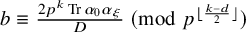 $b \equiv \frac {2 p^k \operatorname {\mathrm {Tr}} \alpha _0 \alpha _\xi }{D} \ \pmod {p^{\lfloor \frac {k-d}{2}\rfloor }}$
. We proceed by cases. Let us write
$b \equiv \frac {2 p^k \operatorname {\mathrm {Tr}} \alpha _0 \alpha _\xi }{D} \ \pmod {p^{\lfloor \frac {k-d}{2}\rfloor }}$
. We proceed by cases. Let us write
 $S(\ell ,n)$
for the number of integers x modulo n for which
$S(\ell ,n)$
for the number of integers x modulo n for which
 $x^2 -\ell \equiv 0 \ \pmod {n}$
.
$x^2 -\ell \equiv 0 \ \pmod {n}$
.
If
 $d=1$
or
$d=1$
or
 $d=0, p\neq 2$
, and k is even, then the congruence in
$d=0, p\neq 2$
, and k is even, then the congruence in
 $S_{L, b}$
is
$S_{L, b}$
is
 $$ \begin{align*}a^2 - \frac{(p^k \operatorname{\mathrm{Tr}} \alpha_0 \alpha_\xi)^2}{D}\equiv m \ \pmod{p^{\lceil k/2 \rceil}}\end{align*} $$
since
 $\operatorname {\mathrm {Tr}}(\alpha _0)=0$
and
$\operatorname {\mathrm {Tr}}(\alpha _0)=0$
and
 $\operatorname {\mathrm {Nm}}(\alpha _0) p^{\lfloor \frac {k-d}{2}\rfloor }\equiv 0 \ \pmod {p^{\lceil k/2 \rceil }}$
in these cases. Thus, by e.g. [Reference Kaplan and PetrowKP17, Lem. 10] we have
$\operatorname {\mathrm {Nm}}(\alpha _0) p^{\lfloor \frac {k-d}{2}\rfloor }\equiv 0 \ \pmod {p^{\lceil k/2 \rceil }}$
in these cases. Thus, by e.g. [Reference Kaplan and PetrowKP17, Lem. 10] we have
 $$ \begin{align*}|S_{L,b}|\leq S(\frac{(p^k \operatorname{\mathrm{Tr}} \alpha_0 \alpha_\xi)^2}{D} +m,p^{\lceil \frac{k}{2}\rceil})\leq 2p^{\lfloor \frac{1}{2} \min(v(\frac{(p^k \operatorname{\mathrm{Tr}} \alpha_0 \alpha_\xi)^2}{D} +m),\lceil \frac{k}{2} \rceil)\rfloor}.\end{align*} $$
Now consider the case that
 $p=2$
. We may complete the square to find that any
$p=2$
. We may complete the square to find that any
 $a \in S_{L, b}$
satisfies
$a \in S_{L, b}$
satisfies
 $$ \begin{align*}\left(a+ \frac{p^k \operatorname{\mathrm{Tr}} \alpha_0 \alpha_\xi}{D} \operatorname{\mathrm{Tr}} \alpha_0\right)^2- \frac{(p^k \operatorname{\mathrm{Tr}} \alpha_0 \alpha_\xi)^2}{D} -m \equiv 0 \ \pmod{p^{\lfloor \frac{k-d}{2}\rfloor}}.\end{align*} $$
Thus,
 $|S_{L,b}|\leq S(\frac {(p^k \operatorname {\mathrm {Tr}} \alpha _0 \alpha _\xi )^2}{D} +m,p^{\lfloor \frac {k-d}{2}\rfloor })$
. Since
$|S_{L,b}|\leq S(\frac {(p^k \operatorname {\mathrm {Tr}} \alpha _0 \alpha _\xi )^2}{D} +m,p^{\lfloor \frac {k-d}{2}\rfloor })$
. Since
 $\lceil \frac {k}{2}\rceil - \lfloor \frac {k-d}{2}\rfloor \leq 2$
, we have by e.g. [Reference Kaplan and PetrowKP17, Lem. 10] that
$\lceil \frac {k}{2}\rceil - \lfloor \frac {k-d}{2}\rfloor \leq 2$
, we have by e.g. [Reference Kaplan and PetrowKP17, Lem. 10] that
 $$ \begin{align*}S(\frac{(p^k \operatorname{\mathrm{Tr}} \alpha_0 \alpha_\xi)^2}{D} +m,p^{\lfloor \frac{k-d}{2}\rfloor}) \leq 4S(\frac{(p^k \operatorname{\mathrm{Tr}} \alpha_0 \alpha_\xi)^2}{D} +m,p^{\lceil \frac{k}{2}\rceil}) \leq 16p^{\lfloor \frac{1}{2} \min(v(\frac{(p^k \operatorname{\mathrm{Tr}} \alpha_0 \alpha_\xi)^2}{D} +m),\lceil \frac{k}{2} \rceil)\rfloor}.\end{align*} $$
Lastly, let us consider the case that
 $d=0$
,
$d=0$
,
 $p \neq 2$
, and k is odd. Writing
$p \neq 2$
, and k is odd. Writing
 $b_0 = \frac {2 p^k \operatorname {\mathrm {Tr}} \alpha _0 \alpha _\xi }{D}$
, we parametrize the possible values of b by
$b_0 = \frac {2 p^k \operatorname {\mathrm {Tr}} \alpha _0 \alpha _\xi }{D}$
, we parametrize the possible values of b by
 $b=b_0+ xp^{\lfloor k/2\rfloor }$
, where x runs modulo p. Then,
$b=b_0+ xp^{\lfloor k/2\rfloor }$
, where x runs modulo p. Then,
 $$ \begin{align*}|S_{L,b}| = S(m-b_0^2\operatorname{\mathrm{Nm}}(\alpha_0)-2xb_0p^{\lfloor k/2 \rfloor}\operatorname{\mathrm{Nm}}(\alpha_0), p^{\lceil k/2 \rceil}).\end{align*} $$
If
 $v(b_0)>0$
, then
$v(b_0)>0$
, then
 $b_0p^{\lfloor k/2 \rfloor } \equiv 0 \ \pmod {p^{\lceil k/2 \rceil }}$
and we have
$b_0p^{\lfloor k/2 \rfloor } \equiv 0 \ \pmod {p^{\lceil k/2 \rceil }}$
and we have
 $$ \begin{align*}|S_{L,b}|\leq 2 p^{\lfloor \frac{1}{2} \min(v(m-b_0^2\operatorname{\mathrm{Nm}}(\alpha_0))),\lceil \frac{k}{2} \rceil)\rfloor}\end{align*} $$
by a direct application of [Reference Kaplan and PetrowKP17, Lem. 10]. So, we may assume
 $v(b_0)=0$
in the following.
$v(b_0)=0$
in the following.
If
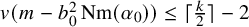 $v(m-b_0^2\operatorname {\mathrm {Nm}}(\alpha _0))\leq \lceil \frac {k}{2}\rceil -2$
, then
$v(m-b_0^2\operatorname {\mathrm {Nm}}(\alpha _0))\leq \lceil \frac {k}{2}\rceil -2$
, then
 $v(m-b_0^2\operatorname {\mathrm {Nm}}(\alpha _0)-2xb_0p^{\lfloor k/2 \rfloor }\operatorname {\mathrm {Nm}}(\alpha _0)) = v(m-b_0^2\operatorname {\mathrm {Nm}}(\alpha _0))$
, so that by loc. cit.
$v(m-b_0^2\operatorname {\mathrm {Nm}}(\alpha _0)-2xb_0p^{\lfloor k/2 \rfloor }\operatorname {\mathrm {Nm}}(\alpha _0)) = v(m-b_0^2\operatorname {\mathrm {Nm}}(\alpha _0))$
, so that by loc. cit.
 $$ \begin{align*}|S_{L,b}| \leq 2p^{\lfloor \frac{1}{2} \min(v(m-b_0^2\operatorname{\mathrm{Nm}}(\alpha_0)),\lceil \frac{k}{2} \rceil)\rfloor}.\end{align*} $$
If
 $v(m-b_0^2\operatorname {\mathrm {Nm}}(\alpha _0))\geq \lceil \frac {k}{2}\rceil -1$
and
$v(m-b_0^2\operatorname {\mathrm {Nm}}(\alpha _0))\geq \lceil \frac {k}{2}\rceil -1$
and
 $\lceil k/2 \rceil $
is odd, then similarly
$\lceil k/2 \rceil $
is odd, then similarly
 $$ \begin{align*}|S_{L,b}| = p^{\frac{1}{2} ( \lceil \frac{k}{2}\rceil -1)} S\left( \frac{m-b_0^2\operatorname{\mathrm{Nm}}(\alpha_0)-2xb_0p^{\lfloor k/2 \rfloor}\operatorname{\mathrm{Nm}}(\alpha_0)}{p^{ \lceil \frac{k}{2}\rceil -1}},p\right)\leq 2 p^{\lfloor \frac{1}{2} \min(v(m-b_0^2\operatorname{\mathrm{Nm}}(\alpha_0))),\lceil \frac{k}{2} \rceil)\rfloor}.\end{align*} $$
If
 $v(m-b_0^2\operatorname {\mathrm {Nm}}(\alpha _0))\geq \lceil \frac {k}{2}\rceil -1$
and
$v(m-b_0^2\operatorname {\mathrm {Nm}}(\alpha _0))\geq \lceil \frac {k}{2}\rceil -1$
and
 $\lceil k/2 \rceil $
is even, then
$\lceil k/2 \rceil $
is even, then
 $$ \begin{align*}|S_{L,b}| = p^{\frac{1}{2} ( \lceil \frac{k}{2}\rceil -2)} S\left( \frac{m-b_0^2\operatorname{\mathrm{Nm}}(\alpha_0)-2xb_0p^{\lfloor k/2 \rfloor}\operatorname{\mathrm{Nm}}(\alpha_0)}{p^{ \lceil \frac{k}{2}\rceil -2}},p^2\right)\end{align*} $$
and
 $$ \begin{align*}v\left(\frac{m-b_0^2\operatorname{\mathrm{Nm}}(\alpha_0)-2xb_0p^{\lfloor k/2 \rfloor}\operatorname{\mathrm{Nm}}(\alpha_0)}{p^{ \lceil \frac{k}{2}\rceil -2}}\right) = \begin{cases} \geq 2 & \text{ if } x = \frac{m-b_0^2\operatorname{\mathrm{Nm}}(\alpha_0)}{2b_0p^{\lfloor k/2 \rfloor}\operatorname{\mathrm{Nm}}(\alpha_0)}, \\ 1 & \text{ otherwise.}\end{cases}\end{align*} $$
Thus by loc. cit.
 $$ \begin{align*}|S_{L,b}| = \begin{cases}p^{\frac{1}{2} \lceil \frac{k}{2}\rceil} & \text{ if } b= \frac{1}{2}(b_0+ \frac{m}{b_0\operatorname{\mathrm{Nm}}(\alpha_0)}), \\ 0 & \text{ otherwise,}\end{cases}\end{align*} $$
and
 $$ \begin{align*}\frac{1}{2} \lceil \frac{k}{2}\rceil =\lceil \frac{1}{2} \min(v(m-b_0^2\operatorname{\mathrm{Nm}}(\alpha_0)),\lceil \frac{k}{2} \rceil)\rceil \leq \lfloor \frac{1}{2} \min(v(m-b_0^2\operatorname{\mathrm{Nm}}(\alpha_0)),\lceil \frac{k}{2} \rceil)\rfloor +1.\end{align*} $$
Of course,
 $m-b_0^2\operatorname {\mathrm {Nm}}(\alpha _0)= m+\frac {(p^k \operatorname {\mathrm {Tr}} \alpha _0 \alpha _\xi )^2}{D}.$
Drawing these cases together, we conclude that
 $$ \begin{align*}|S_L| \leq 2^6 p^{{\mathfrak{a}} + \lfloor \frac{1}{2} \min(v(\frac{(p^k \operatorname{\mathrm{Tr}} \alpha_0 \alpha_\xi)^2}{D} +m),\lceil \frac{k}{2} \rceil)\rfloor},\end{align*} $$
where
 $2^6$
may be replaced by
$2^6$
may be replaced by
 $2$
if
$2$
if
 $p\neq 2$
.
$p\neq 2$
.
Now let us consider the sum U. In similar fashion to the proof of Proposition 6.54, the condition
 $v(\widetilde {b}) \geq \lfloor \frac {k+(e-1)}{2}\rfloor $
excludes all cases except
$v(\widetilde {b}) \geq \lfloor \frac {k+(e-1)}{2}\rfloor $
excludes all cases except
 $d=3,1$
, or (
$d=3,1$
, or (
 $p \neq 2, d=0$
and
$p \neq 2, d=0$
and
 $v(a)=0$
). In these cases, by Table 3 we have that
$v(a)=0$
). In these cases, by Table 3 we have that
 $v(\widetilde {b})= v(b)+(e-1)+v(2)$
. If
$v(\widetilde {b})= v(b)+(e-1)+v(2)$
. If
 $k \geq 2c_0+d$
, then by Proposition 6.51, the sum
$k \geq 2c_0+d$
, then by Proposition 6.51, the sum
 $H_p(m,1,p^k)$
is a classical Kloosterman sum, so that (6.99) holds by the classical Weil bound. We may therefore assume that
$H_p(m,1,p^k)$
is a classical Kloosterman sum, so that (6.99) holds by the classical Weil bound. We may therefore assume that
 $k< 2c_0+d$
for the remainder of the proof.
$k< 2c_0+d$
for the remainder of the proof.
First let us suppose that p is odd, which ensures that all terms in the sum U with
 $v(a) \neq 0$
vanish. Moreover, we have by Lemma 6.52(2) that U vanishes unless
$v(a) \neq 0$
vanish. Moreover, we have by Lemma 6.52(2) that U vanishes unless
 $\lceil (k-(e-1))/2\rceil \geq c_0$
, so that the only case left to consider is when
$\lceil (k-(e-1))/2\rceil \geq c_0$
, so that the only case left to consider is when
 $k=2c_0+e-2$
. Thus, when
$k=2c_0+e-2$
. Thus, when
 $p\neq 2$
and
$p\neq 2$
and
 $k<2c_0+d$
, the sum U either vanishes, or
$k<2c_0+d$
, the sum U either vanishes, or
 $$ \begin{align*}U = p^{-\lceil \frac{3k-d}{2}\rceil } \sum_{\substack{b \in \mathcal{O}/p^{c_0}\mathcal{O} \\ v(b) \geq c_0-1}} \sum_{\substack{a \in (\mathcal{O}/p^{c_0}\mathcal{O})^\times \\ a^2 + b^2 \operatorname{\mathrm{Nm}}(\alpha_0) \equiv m \ \pmod{p^{k}}}} \xi(a+b\alpha_0)\psi(-\frac{2a}{p^{k}}).\end{align*} $$
For
 $m \in \mathcal {O}^\times $
the domain of summation on a is
$m \in \mathcal {O}^\times $
the domain of summation on a is
 $$ \begin{align*} \{a \in (\mathcal{O}/p^{c_0}\mathcal{O})^\times : \exists \text{ a lift } \tilde{a} \in (\mathcal{O}/p^k\mathcal{O})^\times \text{ of } a &\text{ with } \tilde{a}^2 \equiv m-b^2\operatorname{\mathrm{Nm}}(\alpha_0) \ \pmod{p^k}\} \\ & \quad= \{ a \in (\mathcal{O}/p^{c_0}\mathcal{O})^\times : a^2 \equiv m \ \pmod{p^{c_0}}\} \end{align*} $$
by Hensel’s lemma. In particular, the domain is independent of b. The result of these transformations is
 $$ \begin{align*} U&= p^{-\lceil \frac{3k-d}{2}\rceil } \sum_{\substack{a \in (\mathcal{O}/p^{c_0}\mathcal{O})^\times \\ a^2 = m \ \pmod{p^{c_0}}}} \sum_{\substack{b \in \mathcal{O}/p^{c_0}\mathcal{O} \\ v(b) \geq c_0-1}} \xi(a+b\alpha_0)\psi(-\frac{2a}{p^{k}}) \\ & = p^{-\lceil \frac{3k-d}{2}\rceil } \sum_{\substack{a \in (\mathcal{O}/p^{c_0}\mathcal{O})^\times \\ a^2 = m \ \pmod{p^{c_0}}}} \xi(a)\psi(-\frac{2a}{p^{k}}) \sum_{\substack{b \in \mathcal{O}/p^{c_0}\mathcal{O} \\ v(b) \geq c_0-1}} \psi(\frac{b}{a} \operatorname{\mathrm{Tr}} \alpha_\xi \alpha_0) = 0. \end{align*} $$
If
 $d=3$
, then essentially the same argument as for
$d=3$
, then essentially the same argument as for
 $p\neq 2$
goes through to show that
$p\neq 2$
goes through to show that
 $U=0$
when
$U=0$
when
 $k<2c_0+d$
. We quickly note the necessary changes. Lemma 6.52(2) shows that U vanishes, except possibly in the cases
$k<2c_0+d$
. We quickly note the necessary changes. Lemma 6.52(2) shows that U vanishes, except possibly in the cases
 $2c_0\leq k\leq 2c_0+2$
. We have
$2c_0\leq k\leq 2c_0+2$
. We have
 $$ \begin{align*}\begin{cases} b \in \mathcal{O}/p^{c_0}\mathcal{O}, v(b)\geq c_0-2 & \text{ if } k=2c_0, \\ b \in \mathcal{O}/p^{c_0}\mathcal{O}, v(b)\geq c_0-1 & \text{ if } k=2c_0+1, \\ b \in \mathcal{O}/p^{c_0+1}\mathcal{O}, v(b)\geq c_0-1 & \text{ if } k=2c_0+2,\end{cases} \text{ and } a \in \begin{cases} (\mathcal{O}/p^{c_0}\mathcal{O})^\times & \text{ if } k=2c_0, \\ (\mathcal{O}/p^{c_0+1}\mathcal{O})^\times & \text{ if } k\geq 2c_0 +1.\end{cases}\end{align*} $$
Lastly, we use the hypothesis
 $c(\sigma )\geq 9$
from Theorem 6.45 to ensure that
$c(\sigma )\geq 9$
from Theorem 6.45 to ensure that
 $b^2 \operatorname {\mathrm {Nm}}(\alpha _0) \equiv 0 \ \pmod {p^{c_0}}$
and that Hensel’s lemma continues to work in residue characteristic 2.
$b^2 \operatorname {\mathrm {Nm}}(\alpha _0) \equiv 0 \ \pmod {p^{c_0}}$
and that Hensel’s lemma continues to work in residue characteristic 2.
Proposition 6.56 does not apply in the case
 $c(\sigma )=2$
and
$c(\sigma )=2$
and
 $k=1$
(i.e.
$k=1$
(i.e.
 $c_0=1$
and
$c_0=1$
and
 $E/F$
unramified) since the decomposition (6.91) is tautological in that case. Instead, we have the following bounds from
$E/F$
unramified) since the decomposition (6.91) is tautological in that case. Instead, we have the following bounds from
 $\ell $
-adic cohomology.
$\ell $
-adic cohomology.
Proposition 6.58 (Deligne, Katz).
Suppose
 $E/F$
is an unramified quadratic extension,
$E/F$
is an unramified quadratic extension,
 $q=|k_F|$
,
$q=|k_F|$
,
 $c(\xi )\leq 1$
and
$c(\xi )\leq 1$
and
 $\psi \neq 1$
an additive character of F of conductor 0. For all m we have
$\psi \neq 1$
an additive character of F of conductor 0. For all m we have
 $$ \begin{align} \Big| \sum_{\substack{u \in (\mathcal{O}_E/p\mathcal{O}_E)^\times \\ \operatorname{\mathrm{Nm}}(u)\equiv m \ \pmod{p}}} \xi(u) \psi_E(-u p^{-1})\Big| \leq 2 \sqrt{q}. \end{align} $$
Proof. Let
 $\ell $
be a prime invertible in the residue field
$\ell $
be a prime invertible in the residue field
 $k_F$
. Deligne [Reference DeligneDel77, Sommes Trig. Rem. 7.18] suggested and Katz [Reference KatzKat88, 8.8.5 Thm.] proved that there exists a lisse
$k_F$
. Deligne [Reference DeligneDel77, Sommes Trig. Rem. 7.18] suggested and Katz [Reference KatzKat88, 8.8.5 Thm.] proved that there exists a lisse
 $\overline {\mathbb Q}_\ell $
-sheaf
$\overline {\mathbb Q}_\ell $
-sheaf
 $\operatorname {\mathrm {Kl}}(\operatorname {\mathrm {Res}}_{k_E/k_F}\mathbb {G}_m, \psi _E,\xi )$
of rank
$\operatorname {\mathrm {Kl}}(\operatorname {\mathrm {Res}}_{k_E/k_F}\mathbb {G}_m, \psi _E,\xi )$
of rank
 $2$
on
$2$
on
 $\mathbb {G}_{m,k_F}$
, pure of weight 1, with trace function
$\mathbb {G}_{m,k_F}$
, pure of weight 1, with trace function
 $$ \begin{align*}t_{\operatorname{\mathrm{Kl}}(\operatorname{\mathrm{Res}}_{k_E/k_F}\mathbb{G}_m, \psi_E,\xi)} (m) = - \sum_{\substack{u \in k_E^\times \\ \operatorname{\mathrm{Nm}}_{k_E/k_F}(u)=m}}\xi(u)\psi_E(u/p).\end{align*} $$
Then, we have that
 $|t_{\operatorname {\mathrm {Kl}}(\operatorname {\mathrm {Res}}_{k_E/k_F}\mathbb {G}_m, \psi _E,\xi )} (m)| \leq 2 \sqrt {q}$
for all
$|t_{\operatorname {\mathrm {Kl}}(\operatorname {\mathrm {Res}}_{k_E/k_F}\mathbb {G}_m, \psi _E,\xi )} (m)| \leq 2 \sqrt {q}$
for all
 $m \in k_F^\times $
(see e.g. [Reference Fouvry, Kowalski, Michel and SawinFKMS19, (3.4)]). If
$m \in k_F^\times $
(see e.g. [Reference Fouvry, Kowalski, Michel and SawinFKMS19, (3.4)]). If
 $m=0$
the sum clearly vanishes.
$m=0$
the sum clearly vanishes.
7 Examples
7.1 Classical family
Choose
 $c \in \mathbb {Z}_{\geq 0}$
and let
$c \in \mathbb {Z}_{\geq 0}$
and let
 $$ \begin{align} f_{\leq c} = \nu(p^c)1_{ZK_0(p^c)}.\end{align} $$
The function
 $f_{\leq c} \in {\mathcal {H}}_p$
is the classical choice of test function matching [Reference Knightly and LiKL13].
$f_{\leq c} \in {\mathcal {H}}_p$
is the classical choice of test function matching [Reference Knightly and LiKL13].
7.1.1 Geometric and Spectral Assumptions
It is clear that
 $f_{\leq c}$
satisfies Geometric Assumptions (1) and (2) with
$f_{\leq c}$
satisfies Geometric Assumptions (1) and (2) with
 $y=p^{i}$
, any
$y=p^{i}$
, any
 $i \leq c$
. It also satisfies the spectral assumption, by definition.
$i \leq c$
. It also satisfies the spectral assumption, by definition.
7.1.2 Local family
The operator
 $\pi (f_{\leq c}):V_\pi \to V_\pi $
is the orthogonal projection onto the space
$\pi (f_{\leq c}):V_\pi \to V_\pi $
is the orthogonal projection onto the space
 $V_\pi ^{K_0(p^c)}$
of
$V_\pi ^{K_0(p^c)}$
of
 $K_0(p^c)$
-fixed vectors in
$K_0(p^c)$
-fixed vectors in
 $V_\pi $
. Therefore the local family
$V_\pi $
. Therefore the local family
 $\mathcal {F}_{\leq c}:=\mathcal {F}_p(f_{\leq c})$
consists of
$\mathcal {F}_{\leq c}:=\mathcal {F}_p(f_{\leq c})$
consists of
 $\pi \in {\overline {G}}(\mathbb Q_p)^{\wedge }$
that admit a nonzero
$\pi \in {\overline {G}}(\mathbb Q_p)^{\wedge }$
that admit a nonzero
 $K_0(p^c)$
-fixed vector. Equivalently, by newform theory
$K_0(p^c)$
-fixed vector. Equivalently, by newform theory
 $$ \begin{align} \mathcal{F}_{\leq c}= \{ \pi \in {\overline{G}}(\mathbb Q_p)^{\wedge}: c(\pi) \leq c\}. \end{align} $$
7.1.3 Level
It is clear that the local level
 $N_p$
of
$N_p$
of
 $f_{\leq c}$
satisfies
$f_{\leq c}$
satisfies
 $N_p = p^c$
.
$N_p = p^c$
.
7.1.4 Diagonal weights
By definition
 $$ \begin{align} \delta_p:= \int_{c(\pi) \leq c} \dim V_\pi^{K_0(p^c)}\, d\widehat{\mu}(\pi) = \int_{{\overline{G}(\mathbb Q_p)}^{\wedge}} \operatorname{\mathrm{Tr}} \pi(f_{\leq c})\,d\widehat{\mu}(\pi), \end{align} $$
which by the Plancherel formula equals
 $$ \begin{align} \int_{\mathbb Q_p} f_{\leq c} \left( \begin{smallmatrix} 1 & t \\ 0 & 1 \end{smallmatrix} \right) \psi_p(-mt)\,dt = \nu(p^c) = f_{\leq c}(1) \end{align} $$
for any
 $m \in \mathbb {Z}_p^\times $
.
$m \in \mathbb {Z}_p^\times $
.
7.1.5 Local Generalized Kloosterman Sums
We have that
 $$ \begin{align} H_p(m,n;p^k) = \begin{cases} 0 & \text{ if } k< c, \\ \delta_p S(m,n;p^k) & \text{ if } k \geq c \end{cases} \end{align} $$
by e.g. [Reference Knightly and LiKL06a, Prop. 3.7].
7.1.6 Local Geometric Conductor
Equation (7.5) shows that the local geometric conductor
 $k_p$
satisfies
$k_p$
satisfies
 $k_p=c$
by the generic nonvanishing of classical Kloosterman sums.
$k_p=c$
by the generic nonvanishing of classical Kloosterman sums.
7.1.7 Hypotheses from Section 1.5
Hypothesis 1.21 (CvF) holds for the classical family
 $\mathcal {F}_{\leq c}$
, since
$\mathcal {F}_{\leq c}$
, since
 $p^{k_p} = p^c \geq \frac {2}{3} \nu (p^c) =\frac {2}{3} f_{\leq c}(1).$
To verify Hypothesis 1.20 (FTB), we compute the Fourier/Mellin transform of
 $H_p$
. A simple calculation shows that when
$H_p$
. A simple calculation shows that when
 $k\geq c$
and
$k\geq c$
and
 $c(\chi )\leq k$
 $$ \begin{align} \widehat{H}_p(\chi,k) := \frac{1}{\varphi(p^k)}\sideset{}{^*}\sum_{m \ \pmod{p^k}} H_p(m,1;p^k)\overline{\chi(m)} = \nu(p^c) \frac{\tau(\overline{\chi})^2}{\varphi(p^k)}, \end{align} $$
where
 $$ \begin{align*}\tau(\chi) = \sideset{}{^*}\sum_{m \ \pmod{q}}\chi(m) e(m/q)\end{align*} $$
is the classical Gauss sum of
 $\chi $
as in e.g. [Reference Petrow and YoungPY23, Lem. 7.1]. In particular, we have
$\chi $
as in e.g. [Reference Petrow and YoungPY23, Lem. 7.1]. In particular, we have
 $$ \begin{align*}|\widehat{H}_p(\chi,k)| = \begin{cases} 0 & \text{ if } k<c, \\ f_{\leq c}(1) \zeta_p(1) & \text{ if } c(\chi) = k \geq c, \\ f_{\leq c}(1) \zeta_p(1) p^{-1} & \text{ if } c(\chi)=0 \text{ and } k=1\geq c, \\ 0 & \text{ if } 0<c(\chi)< k \text{ and } k\geq c, \\ 0 & \text{ if } c(\chi)=0 \text{ and } k\geq 2, \end{cases}\end{align*} $$
so that Hypothesis 1.20 (FTB) follows. As a side comment, the sum in (7.6) is meaningless if
 $c(\chi )>k$
, but the integral in (1.49) for
$c(\chi )>k$
, but the integral in (1.49) for
 $\widehat {H}_p(\chi ,k)$
does make sense and returns 0 for
$\widehat {H}_p(\chi ,k)$
does make sense and returns 0 for
 $c(\chi )>k$
.
$c(\chi )>k$
.
7.2 Principal series families
Let
 $\chi $
be a character of
$\chi $
be a character of
 $\mathbb {Z}_p^\times $
with
$\mathbb {Z}_p^\times $
with
 $\chi ^2$
nontrivial, i.e. a primitive nonquadratic Dirichlet character to some p-power modulus. Write
$\chi ^2$
nontrivial, i.e. a primitive nonquadratic Dirichlet character to some p-power modulus. Write
 $c=c(\chi )$
, and if
$c=c(\chi )$
, and if
 $p=2$
assume in addition that
$p=2$
assume in addition that
 $c\geq 4$
. We define a test function
$c\geq 4$
. We define a test function
 $f_\chi \in {\mathcal {H}}_p$
by
$f_\chi \in {\mathcal {H}}_p$
by
 $$ \begin{align} f_\chi(g) := \frac{1}{\varphi(p^c)}\sum_{a,a' \in (\mathbb{Z}/p^c\mathbb{Z})^{\times}} f_{\chi, a,a'} , \end{align} $$
where
 $$ \begin{align} f_{\chi, a,a'} = \chi(a)^{-1} \chi(a') f_{\chi,0}(n(a'p^{-c})^{-1} g n(a p^{-c})), \end{align} $$
and
 $$ \begin{align} f_{\chi,0} (g) := \nu(p^c) 1_{ZK_0(p^c)} \overline{\chi(\alpha/\delta)} \quad \text{ for } \quad g= \left(\begin{smallmatrix} \alpha & \beta \\ \gamma & \delta \end{smallmatrix}\right) \in G(\mathbb Q_p). \end{align} $$
Note in particular that
 $f_\chi (1)=f_{\chi ,0}(1) = \nu (p^c)$
.
$f_\chi (1)=f_{\chi ,0}(1) = \nu (p^c)$
.
As we will see, the relative trace formula Theorem 1.8 associated to the choice
 $f_\chi $
at all ramified places matches the Bruggeman-Kuznetsov trace formula for
$f_\chi $
at all ramified places matches the Bruggeman-Kuznetsov trace formula for
 $\cup _{m \mid q} ({\mathcal {H}}(m, \chi ^2) \otimes \overline {\chi })$
derived by classical means by the second and third authors in [Reference Petrow and YoungPY20] (here
$\cup _{m \mid q} ({\mathcal {H}}(m, \chi ^2) \otimes \overline {\chi })$
derived by classical means by the second and third authors in [Reference Petrow and YoungPY20] (here
 ${\mathcal {H}}(m,\chi ^2)$
is a basis of Hecke-Maass newforms of level
${\mathcal {H}}(m,\chi ^2)$
is a basis of Hecke-Maass newforms of level
 $m \mid q$
and central character
$m \mid q$
and central character
 $\chi ^2$
, where
$\chi ^2$
, where
 $\chi $
is a primitive Dirichlet character modulo q). Note that in [Reference Petrow and YoungPY20], the family used had
$\chi $
is a primitive Dirichlet character modulo q). Note that in [Reference Petrow and YoungPY20], the family used had
 ${\mathcal {H}}(m, \overline {\chi }^2) \otimes \chi $
instead of
${\mathcal {H}}(m, \overline {\chi }^2) \otimes \chi $
instead of
 ${\mathcal {H}}(m, \chi ^2) \otimes \overline {\chi }$
, but of course these are identical.
${\mathcal {H}}(m, \chi ^2) \otimes \overline {\chi }$
, but of course these are identical.
7.2.1 Geometric and Spectral Assumptions
We can check by an explicit calculation that for any
 $\alpha ,\alpha ' \in (\mathbb {Z}/p^c\mathbb {Z})^\times $
, the support of
$\alpha ,\alpha ' \in (\mathbb {Z}/p^c\mathbb {Z})^\times $
, the support of
 $f_{\chi , 0}(n(\alpha 'p^{-c})^{-1} g n(\alpha p^{-c}))$
is contained in
$f_{\chi , 0}(n(\alpha 'p^{-c})^{-1} g n(\alpha p^{-c}))$
is contained in
 $a(p^c)^{-1}Z K_p a(p^c)$
. Therefore,
$a(p^c)^{-1}Z K_p a(p^c)$
. Therefore,
 $f_\chi $
satisfies Geometric Assumption (2) with
$f_\chi $
satisfies Geometric Assumption (2) with
 $y=p^{c}$
.
$y=p^{c}$
.
In the case that p is odd, the spectral assumption for
 $f_\chi $
was established by the first named author [Reference HuHu24, §3.3]. Precisely, by Proposition 3.28 and the first sentence of Corollary 3.24 of loc. cit. we have that
$f_\chi $
was established by the first named author [Reference HuHu24, §3.3]. Precisely, by Proposition 3.28 and the first sentence of Corollary 3.24 of loc. cit. we have that
 $\pi (f_\chi ):V_\pi \to V_\pi $
is an orthogonal projection onto the line of the newform in
$\pi (f_\chi ):V_\pi \to V_\pi $
is an orthogonal projection onto the line of the newform in
 $V_\pi $
if
$V_\pi $
if
 $\pi $
is isomorphic to a principal series representation
$\pi $
is isomorphic to a principal series representation
 $\pi (\mu ,\mu ^{-1})$
with
$\pi (\mu ,\mu ^{-1})$
with
 $\mu \vert _{\mathbb {Z}_p^\times } = \chi $
and
$\mu \vert _{\mathbb {Z}_p^\times } = \chi $
and
 $\pi (f_\chi )= 0$
if
$\pi (f_\chi )= 0$
if
 $\pi $
is not such a representation (recall we have assumed that
$\pi $
is not such a representation (recall we have assumed that
 $\chi $
is not quadratic). Therefore
$\chi $
is not quadratic). Therefore
 $f_\chi $
is a newform projector, and hence satisfies the spectral assumption.
$f_\chi $
is a newform projector, and hence satisfies the spectral assumption.
If
 $p=2$
then we may argue along similar lines to show that
$p=2$
then we may argue along similar lines to show that
 $f_\chi $
is a newform projector. We briefly give the details now. First, note that
$f_\chi $
is a newform projector. We briefly give the details now. First, note that
 $c(\chi ^2) = c-1$
since we have assumed
$c(\chi ^2) = c-1$
since we have assumed
 $c\geq 4$
, as can be seen by e.g. Lemma 6.1. Next, denote by
$c\geq 4$
, as can be seen by e.g. Lemma 6.1. Next, denote by
 $\tilde {\theta }'$
the function on
$\tilde {\theta }'$
the function on
 $ZK_0(p^{c})$
given by
$ZK_0(p^{c})$
given by
 $$ \begin{align*}\tilde{\theta}'\left(\begin{smallmatrix} \alpha & \beta \\ \gamma & \delta \end{smallmatrix} \right)=\chi^{-2}(\delta).\end{align*} $$
Lemma 7.1. Let
 $\pi '$
be an irreducible smooth admissible representation of
$\pi '$
be an irreducible smooth admissible representation of
 $\operatorname {\mathrm {GL}}_2(\mathbb Q_2)$
and
$\operatorname {\mathrm {GL}}_2(\mathbb Q_2)$
and
 $c\geq 4$
. Then the subspace of
$c\geq 4$
. Then the subspace of
 $V_{\pi '}$
on which
$V_{\pi '}$
on which
 $ZK_0(p^{c})$
acts by the character
$ZK_0(p^{c})$
acts by the character
 $\tilde {\theta }'$
is nontrivial only when
$\tilde {\theta }'$
is nontrivial only when
 $\pi '\simeq \pi (\nu ,\nu ^{-1}\chi ^{-2})$
for some unramified character
$\pi '\simeq \pi (\nu ,\nu ^{-1}\chi ^{-2})$
for some unramified character
 $\nu $
, in which case it is two dimensional with a basis given by the newform
$\nu $
, in which case it is two dimensional with a basis given by the newform
 $\varphi _0'\in V_{\pi '}$
and its translate
$\varphi _0'\in V_{\pi '}$
and its translate
 $\varphi _1'=\pi '(a(p))\varphi _0'$
.
$\varphi _1'=\pi '(a(p))\varphi _0'$
.
Proof. If the subspace of
 $V_{\pi '}$
on which
$V_{\pi '}$
on which
 $K_0(p^{c})$
acts by the character
$K_0(p^{c})$
acts by the character
 $\tilde {\theta }'$
is nontrivial, it is necessary that
$\tilde {\theta }'$
is nontrivial, it is necessary that
 $\pi '=\pi (\eta _1,\eta _2)$
(see e.g. [Reference CasselmanCas73b, Pf. of Prop. 2]) with
$\pi '=\pi (\eta _1,\eta _2)$
(see e.g. [Reference CasselmanCas73b, Pf. of Prop. 2]) with
 $\sum c(\eta _i)\leq c$
and
$\sum c(\eta _i)\leq c$
and
 $c(\eta _1\eta _2)=c-1$
. As there is no character over
$c(\eta _1\eta _2)=c-1$
. As there is no character over
 $\mathbb Q_2$
with level
$\mathbb Q_2$
with level
 $1$
, and the central character is determined, we have
$1$
, and the central character is determined, we have
 $\pi '\simeq \pi (\nu ,\nu ^{-1}\chi ^{-2})$
for some unramified characters
$\pi '\simeq \pi (\nu ,\nu ^{-1}\chi ^{-2})$
for some unramified characters
 $\nu $
. In that case we have
$\nu $
. In that case we have
 $c(\pi ')=c(\chi )-1$
, thus by newform theory the corresponding subspace is 2-dimensional, spanned by the newform and its diagonal translate.
$c(\pi ')=c(\chi )-1$
, thus by newform theory the corresponding subspace is 2-dimensional, spanned by the newform and its diagonal translate.
Now we twist back. Denote by
 $\tilde {\theta }$
the following character on
$\tilde {\theta }$
the following character on
 $ZK_0(p^{c})$
 $$ \begin{align} \tilde{\theta}\left(\begin{smallmatrix} \alpha & \beta \\ \gamma & \delta \end{smallmatrix}\right)=\chi(\alpha/\delta). \end{align} $$
Lemma 7.2. Let
 $\pi $
be an irreducible smooth admissible representation of
$\pi $
be an irreducible smooth admissible representation of
 $\operatorname {\mathrm {GL}}_2(\mathbb Q_2)$
and
$\operatorname {\mathrm {GL}}_2(\mathbb Q_2)$
and
 $c\geq 4$
. Then the subspace of
$c\geq 4$
. Then the subspace of
 $V_\pi $
on which
$V_\pi $
on which
 $ZK_0(p^{c})$
acts by the character
$ZK_0(p^{c})$
acts by the character
 $\tilde {\theta }$
is nontrivial only when
$\tilde {\theta }$
is nontrivial only when
 $\pi \simeq \pi (\nu \chi ,\nu ^{-1}\chi ^{-1})$
for some unramified characters
$\pi \simeq \pi (\nu \chi ,\nu ^{-1}\chi ^{-1})$
for some unramified characters
 $\nu $
, in which case it is two dimensional with a basis
$\nu $
, in which case it is two dimensional with a basis
 $\{\varphi _0,\varphi _1\}$
given in the Whittaker model by
$\{\varphi _0,\varphi _1\}$
given in the Whittaker model by
 $$ \begin{align*}W_0\left(\begin{pmatrix} x & 0 \\ 0 & 1 \end{pmatrix}\right) &=\sqrt{1-p^{-1}}\begin{cases} p^{-v \left( x \right) /2}\chi\nu(x), &\text{ if } v \left( x \right) \geq 0,\\ 0, &\text{ otherwise.} \end{cases}\\W_1\left(\begin{pmatrix} x & 0 \\ 0 & 1 \end{pmatrix}\right) &=\sqrt{1-p^{-1}}\begin{cases} p^{-(v \left( x \right) +1) /2}\chi\nu(x), &\text{ if } v \left( x \right) \geq -1,\\ 0, &\text{ otherwise.} \end{cases}\end{align*} $$
A similar statement to Lemma 7.2 was previously given by Nelson [Reference NelsonNel18, Lem. 48].
The following is an analogue of [Reference HuHu24, Lem. 3.25]:
Lemma 7.3. For
 $\pi $
as in Lemma 7.2 and
$\pi $
as in Lemma 7.2 and
 $i=0,1$
,
$i=0,1$
,
 $$ \begin{align*}\sum\limits_{a\in (\mathbb{Z}/p^{c}\mathbb{Z})^\times}\chi(a)\pi\left( \begin{pmatrix} 1 & \frac{a}{p^{c}} \\ 0 & 1 \end{pmatrix}\right) W_{i}\end{align*} $$
is a nonzero scalar multiple of the newform in
 $V_\pi $
.
$V_\pi $
.
Proof. The proof is essentially the same as for [Reference HuHu24, Lem. 3.25] using the Whittaker functions from Lemma 7.2, with the main step being that the Gauss sum
 $$ \begin{align*} \sum\limits_{a\in \left( \mathbb{Z}/p^{c}\mathbb{Z} \right) ^\times}\psi\left(\frac{a x }{p^{c_1}}\right) \chi \left( a x \right) \end{align*} $$
is nonvanishing only if
 $v(x)=0$
, in which case the value is independent of x.
$v(x)=0$
, in which case the value is independent of x.
For the purpose of comparison with [Reference HuHu24], note that
 $$ \begin{align*}f_{\chi,0} = \nu(p^c) \overline{\widetilde{\Phi}}_{0,0} = \frac{1}{\operatorname{\mathrm{vol}}(ZK_0(p^c)/Z)} \overline{\widetilde{\Phi}}_{0,0}, \, \text{ and } \, f_{\chi, a,a'} = \nu(p^c) \overline{\widetilde{\Phi}}_{a,a'}= \frac{1}{\operatorname{\mathrm{vol}}(ZK_0(p^c)/Z)} \overline{\widetilde{\Phi}}_{a,a'},\end{align*} $$
where
 $\widetilde {\Phi }_{0,0}$
and
$\widetilde {\Phi }_{0,0}$
and
 $\widetilde {\Phi }_{a,a'}$
are as in Definition 3.26 of loc. cit.. Recall that
$\widetilde {\Phi }_{a,a'}$
are as in Definition 3.26 of loc. cit.. Recall that
 $\pi $
is unitary with the pairing
$\pi $
is unitary with the pairing
 $\langle \cdot , \cdot \rangle $
given in the Kirillov model by (6.28).
$\langle \cdot , \cdot \rangle $
given in the Kirillov model by (6.28).
Lemma 7.4. For
 $\pi $
as in Lemma 7.2 and
$\pi $
as in Lemma 7.2 and
 $u = n(\alpha p^{-c})$
with
$u = n(\alpha p^{-c})$
with
 $\alpha \not \equiv 0 \ \pmod {p^c}$
,
$\alpha \not \equiv 0 \ \pmod {p^c}$
,
-
(1)
$\text {Span}\{\pi (u)\varphi _0,\pi (u)\varphi _1\}\perp \text {Span}\{\varphi _0,\varphi _1\},$
and -
(2) if
$v\perp \text {Span}\{\varphi _0,\varphi _1\}$
, then
$v\in \ker \pi \left (f_{\chi ,0}\right )$
.


Proof. To verify (1), one can use the unitary pairing
 $\langle \cdot , \cdot \rangle $
on the Kirillov model and the expression of Whittaker functions from Lemma 7.2. To see (2), we note that
$\langle \cdot , \cdot \rangle $
on the Kirillov model and the expression of Whittaker functions from Lemma 7.2. To see (2), we note that
 $$ \begin{align*} \langle \varphi_i, v \rangle = \langle \pi\left(f_{\chi,0}\right) \varphi_i, v \rangle = \langle \varphi_i,\pi\left(f_{\chi,0}\right) v\rangle, \end{align*} $$
where the last equality follows from the fact that
 $\tilde {\theta }$
is a character on the support with
$\tilde {\theta }$
is a character on the support with
 $|\tilde {\theta }|=1$
. Thus
$|\tilde {\theta }|=1$
. Thus
 $v\perp \text {Span}\{\varphi _0,\varphi _1\}$
if and only if
$v\perp \text {Span}\{\varphi _0,\varphi _1\}$
if and only if
 $\pi \left (f_{\chi ,0}\right ) v\perp \text {Span}\{\varphi _0,\varphi _1\}$
, if and only if
$\pi \left (f_{\chi ,0}\right ) v\perp \text {Span}\{\varphi _0,\varphi _1\}$
, if and only if
 $\pi \left (f_{\chi ,0}\right )=0$
. The last equivalence follows from the fact that
$\pi \left (f_{\chi ,0}\right )=0$
. The last equivalence follows from the fact that
 $\langle \cdot ,\cdot \rangle $
is nondegenerate on
$\langle \cdot ,\cdot \rangle $
is nondegenerate on
 $\operatorname {\mathrm {Im}} \pi \left (f_{\chi ,0}\right )$
. Indeed by Lemma 7.2 we have
$\operatorname {\mathrm {Im}} \pi \left (f_{\chi ,0}\right )$
. Indeed by Lemma 7.2 we have
 $$ \begin{align*}\begin{pmatrix} \langle W_0,W_0\rangle & \langle W_0,W_1\rangle \\ \langle W_1,W_0\rangle & \langle W_1,W_1\rangle \end{pmatrix}=\begin{pmatrix} 1 & p^{-1/2} \\ p^{-1/2} & 1 \end{pmatrix} \end{align*} $$
which has nonzero determinant and is thus nondegenerate.
Lemma 7.5.
 $$ \begin{align*}f_{\chi,a,a'}*f_{\chi,b,b'}=\begin{cases} f_{\chi,b,a'} & \text{ if }a\equiv b'\ \pmod{ p^{c}},\\ 0 & \text{ otherwise}. \end{cases}\end{align*} $$
Proof. By definition and change of variable,
 $$ \begin{align*} &f_{\chi,a,a'}*f_{\chi,b,b'}(g)\\ &\quad=\overline{\chi}\left(\frac{ab}{a'b'}\right)\int\limits_{h\in G}f_{\chi,0}\left(\begin{pmatrix} 1 & -a'p^{-c} \\ 0 & 1 \end{pmatrix} gh^{-1}\begin{pmatrix} 1 & ap^{-c} \\ 0 & 1 \end{pmatrix} \right)f_{\chi,0}\left(\begin{pmatrix} 1 & -b'p^{-c} \\ 0 & 1 \end{pmatrix} h\begin{pmatrix} 1 & bp^{-c} \\ 0 & 1 \end{pmatrix}\right)dh\\ &\quad=\overline{\chi}\left(\frac{ab}{a'b'}\right)\int\limits_{h\in G}f_{\chi,0}\left(\begin{pmatrix} 1 & -a'p^{-c} \\ 0 & 1 \end{pmatrix} g\begin{pmatrix} 1 & bp^{-c} \\ 0 & 1 \end{pmatrix}h^{-1} \right)f_{\chi,0}\left(\begin{pmatrix} 1 & (a-b')p^{-c} \\ 0 & 1 \end{pmatrix}h \right)dh. \end{align*} $$
The conclusion is clear when
 $a\equiv b'\ \pmod { p^{c}}$
. We need to show that when
$a\equiv b'\ \pmod { p^{c}}$
. We need to show that when
 $a \not \equiv b' \ \pmod {p^{c}}$
, the integral is always vanishing for any g, i.e.
$a \not \equiv b' \ \pmod {p^{c}}$
, the integral is always vanishing for any g, i.e.
 $$ \begin{align*}f_{\chi,0}*f_{\chi,0,b'-a}=0. \end{align*} $$
By the Plancherel formula (4.3), it suffices to prove that
 $$ \begin{align*}\pi\left(f_{\chi,0}*f_{\chi,0,b'-a}\right)=\pi\left(f_{\chi,0}\right)\pi\left(f_{\chi,0,b'-a}\right)\end{align*} $$
is vanishing for any
 $\pi $
. From Lemma 7.2, we can restrict to the case
$\pi $
. From Lemma 7.2, we can restrict to the case
 $\pi \simeq \pi (\nu \chi ,\nu ^{-1}\chi ^{-1})$
. In this case let
$\pi \simeq \pi (\nu \chi ,\nu ^{-1}\chi ^{-1})$
. In this case let
 $\varphi _0,\varphi _1$
be as in Lemma 7.2. Then by a change of variable,
$\varphi _0,\varphi _1$
be as in Lemma 7.2. Then by a change of variable,
 $$ \begin{align*}\operatorname{\mathrm{Im}}\left(\pi\left(f_{\chi,0,b'-a}\right)\right)=\text{Span}\{\pi(u)\varphi_0,\pi(u)\varphi_1\} \end{align*} $$
for the unipotent matrix
 $$ \begin{align*}u=\begin{pmatrix} 1 & (b'-a)p^{-c} \\ 0 & 1 \end{pmatrix}.\end{align*} $$
The required vanishing now follows from Lemma 7.4.
Proposition 7.6. If
 $\pi \simeq \pi (\mu ,\mu ^{-1})$
with
$\pi \simeq \pi (\mu ,\mu ^{-1})$
with
 $\mu \vert _{\mathbb {Z}_p^\times } = \chi $
, then
$\mu \vert _{\mathbb {Z}_p^\times } = \chi $
, then
 $\pi (f_\chi )$
is a projection operator onto the space of newforms in
$\pi (f_\chi )$
is a projection operator onto the space of newforms in
 $V_\pi $
, and otherwise
$V_\pi $
, and otherwise
 $\pi (f_\chi )=0$
.
$\pi (f_\chi )=0$
.
Proof. First, note that
 $f_\chi *f_\chi =f_\chi $
by the definition of
$f_\chi *f_\chi =f_\chi $
by the definition of
 $f_\chi $
and Lemma 7.5. Thus,
$f_\chi $
and Lemma 7.5. Thus,
 $\pi (f_\chi )$
is a projection operator. Next, note that for any
$\pi (f_\chi )$
is a projection operator. Next, note that for any
 $v\in V_\pi $
,
$v\in V_\pi $
,
 $$ \begin{align} \pi(f_\chi)v = \frac{1}{\varphi(p^c)}\sum_{a' \in (\mathbb{Z}/p^c\mathbb{Z})^{\times}} \chi(a') \pi(n(a'p^{-c})) \pi(f_{\chi,0}) \sum_{a \in (\mathbb{Z}/p^c\mathbb{Z})^{\times}} \chi(a)^{-1}\pi(n(-a p^{-c}))v.\end{align} $$
Note that
 $ZK_0(p^c)$
acts on
$ZK_0(p^c)$
acts on
 $\operatorname {\mathrm {Im}} \pi (f_{\chi , 0})$
through the character
$\operatorname {\mathrm {Im}} \pi (f_{\chi , 0})$
through the character
 $\widetilde {\theta }$
, so by Lemma 7.2
$\widetilde {\theta }$
, so by Lemma 7.2
 $\pi (f_\chi )=0$
unless
$\pi (f_\chi )=0$
unless
 $\pi \simeq \pi (\mu ,\mu ^{-1})$
with
$\pi \simeq \pi (\mu ,\mu ^{-1})$
with
 $\mu \vert _{\mathbb {Z}_p^\times } = \chi $
. If
$\mu \vert _{\mathbb {Z}_p^\times } = \chi $
. If
 $\pi $
is such a principal series, then by Lemmas 7.2 and 7.3, the operator
$\pi $
is such a principal series, then by Lemmas 7.2 and 7.3, the operator
 $\pi (f_\chi )$
has image in the line of the newform. Lastly, choose any
$\pi (f_\chi )$
has image in the line of the newform. Lastly, choose any
 $a_0 \in (\mathbb {Z}/p^c\mathbb {Z})^\times $
and let
$a_0 \in (\mathbb {Z}/p^c\mathbb {Z})^\times $
and let
 $v_0 = \pi (n(a_0p^{-c}))\varphi _0$
. We have by Lemma 7.4 that
$v_0 = \pi (n(a_0p^{-c}))\varphi _0$
. We have by Lemma 7.4 that
 $$ \begin{align*}\pi(f_{\chi,0})\sum_{a \in (\mathbb{Z}/p^c\mathbb{Z})^{\times}} \chi(a)^{-1}\pi(n(-a p^{-c}))v_0 = \chi(a_0)^{-1} \pi(f_{\chi,0})\varphi_0\end{align*} $$
and
 $\pi (f_{\chi ,0})\varphi _0 = \varphi _0$
, so that
$\pi (f_{\chi ,0})\varphi _0 = \varphi _0$
, so that
 $$ \begin{align*}\pi(f_\chi)v_0 = \frac{\chi(a_0)^{-1}}{\varphi(p^c)}\sum_{a' \in (\mathbb{Z}/p^c\mathbb{Z})^{\times}} \chi(a') \pi(n(a'p^{-c}))\varphi_0,\end{align*} $$
which is nonzero by Lemma 7.3.
By Lemma 4.6(2),
 $f_\chi $
also satisfies Geometric Assumption (1).
$f_\chi $
also satisfies Geometric Assumption (1).
7.2.2 Local family
Given
 $\chi $
a character as above, define
$\chi $
a character as above, define
 $$ \begin{align} \mathcal{F}_\chi := \{ \pi(\mu,\mu^{-1}) \in {\overline{G}}^{\wedge}: \mu \vert_{\mathbb{Z}_p^\times} = \chi\}. \end{align} $$
By the discussion in Section 7.2.1, we have that the local family
 $\mathcal {F}_p(f_\chi ) = \mathcal {F}_\chi $
.
$\mathcal {F}_p(f_\chi ) = \mathcal {F}_\chi $
.
7.2.3 Level
The local level
 $N_p$
of
$N_p$
of
 $f_{\chi }$
satisfies
$f_{\chi }$
satisfies
 $N_p = p^{2c}$
. Indeed, since
$N_p = p^{2c}$
. Indeed, since
 $f_\chi $
is a newform projector, Proposition 4.1 applies, and
$f_\chi $
is a newform projector, Proposition 4.1 applies, and
 $f_\chi $
is bi-
$f_\chi $
is bi-
 $K_0(p^{2c})$
-invariant as
$K_0(p^{2c})$
-invariant as
 $c(\pi (\mu ,\mu ^{-1}))=2c$
. Thus,
$c(\pi (\mu ,\mu ^{-1}))=2c$
. Thus,
 $f_\chi $
is bi-
$f_\chi $
is bi-
 $K(p^{2c})$
-invariant and so
$K(p^{2c})$
-invariant and so
 $N_p \mid p^{2c}$
. On the other hand, suppose
$N_p \mid p^{2c}$
. On the other hand, suppose
 $f_\chi $
were bi-
$f_\chi $
were bi-
 $K( p^{2c-1})$
-invariant. Then, it would be bi-invariant by the product
$K( p^{2c-1})$
-invariant. Then, it would be bi-invariant by the product
 $K(p^{2c-1})K_0(p^{2c})= K_0(p^{2c-1})$
. Indeed, the inclusion
$K(p^{2c-1})K_0(p^{2c})= K_0(p^{2c-1})$
. Indeed, the inclusion
 $\subseteq $
is clear and for the other direction, note that
$\subseteq $
is clear and for the other direction, note that
 $$ \begin{align*}\begin{pmatrix} 1 & 0 \\ \frac{c}{a}p^{2c-1} & 1-\frac{bc}{ad} p^{2c-1} \end{pmatrix}\begin{pmatrix} a & b \\ 0 & d \end{pmatrix}= \begin{pmatrix} a & b \\ cp^{2c-1} & d \end{pmatrix} =g\end{align*} $$
for any
 $g \in K_0(p^{2c-1})$
. But then
$g \in K_0(p^{2c-1})$
. But then
 $\pi (f_\chi )V_\pi $
for
$\pi (f_\chi )V_\pi $
for
 $\pi \simeq \pi (\mu ,\mu ^{-1})$
would have a nonzero
$\pi \simeq \pi (\mu ,\mu ^{-1})$
would have a nonzero
 $K_0(p^{2c-1})$
-fixed vector, which it does not. Thus
$K_0(p^{2c-1})$
-fixed vector, which it does not. Thus
 $N_p=p^{2c}$
.
$N_p=p^{2c}$
.
7.2.4 Diagonal weights
By definition,
 $$ \begin{align} \delta_p:= \int_{\mathcal{F}_\chi} \frac{1}{\mathcal{L}_\pi(1)}\, d\widehat{\mu}(\pi) = (1-p^{-1})^{-1} \widehat{\mu}(\mathcal{F}_\chi), \end{align} $$
since
 $\mathcal {L}_\pi (1)= (1-p^{-1})$
is constant on
$\mathcal {L}_\pi (1)= (1-p^{-1})$
is constant on
 $\mathcal {F}_\chi $
, as
$\mathcal {F}_\chi $
, as
 $c(\pi )\geq 2$
for all
$c(\pi )\geq 2$
for all
 $\pi \in \mathcal {F}_\chi $
(recall (1.14) for the definition) By the Plancherel formula,
$\pi \in \mathcal {F}_\chi $
(recall (1.14) for the definition) By the Plancherel formula,
 $$ \begin{align} \delta_p = (1-p^{-1})^{-1} f_\chi(1) = \frac{\nu(p^c)}{1-p^{-1}}. \end{align} $$
7.2.5 Local Generalized Kloosterman Sums
The local generalized Kloosterman sums
 $H_p(m,n;c)$
associated to
$H_p(m,n;c)$
associated to
 $f_\chi $
were computed in [Reference HuHu24, Cor. 4.12] and go through in the case
$f_\chi $
were computed in [Reference HuHu24, Cor. 4.12] and go through in the case
 $p=2$
. We have
$p=2$
. We have
 $$ \begin{align} H_p(m,n;p^k) = \begin{cases}\delta_p \overline{\chi(m)} \chi(n) S_{\chi^2}(m,n;p^k) & \text{ if } k \geq c(\chi) \text{ and } (p,mn)=1, \\ 0 & \text{ if } k<c(\chi) \text{ or } p \mid mn.\end{cases} \end{align} $$
For comparison to the supercuspidal Kloosterman sums below, it is pleasing to note that
 $$ \begin{align} \overline{\chi(m)} \chi(n) S_{\chi^2}(m,n;p^k) = \sideset{}{^*}\sum_{\substack{x,y \ \pmod{p^k} \\ xy =mn}} \overline{\chi(x)}\chi(y)e\left( \frac{x+y}{p^k}\right).\end{align} $$
Remark 7.7. Note that the formula (7.15) for the generalized Kloosterman sums differs from the Kloosterman sums that appear via the classical procedure (as in [Reference Petrow and YoungPY20]) by the factor of
 $(1-p^{-1})$
. The extra factor of
$(1-p^{-1})$
. The extra factor of
 $(1-p^{-1})^{-1}$
may be accounted for by the observation that the harmonic weights in Theorem 1.8 and the harmonic weights in the classically derived formula are not exactly the same. The former are attached to forms of conductor
$(1-p^{-1})^{-1}$
may be accounted for by the observation that the harmonic weights in Theorem 1.8 and the harmonic weights in the classically derived formula are not exactly the same. The former are attached to forms of conductor
 $2c$
and trivial central character, while the latter are attached to forms of level c and nontrivial central character.
$2c$
and trivial central character, while the latter are attached to forms of level c and nontrivial central character.
7.2.6 Local Geometric Conductor
The previous subsection shows that the local geometric conductor
 $k_p$
satisfies
$k_p$
satisfies
 $k_p=c$
by the generic nonvanishing of classical Kloosterman sums.
$k_p=c$
by the generic nonvanishing of classical Kloosterman sums.
7.2.7 Hypotheses from Section 1.5
Hypothesis 1.21 (CvF) holds for the family
 $\mathcal {F}_{\chi }$
, since
$\mathcal {F}_{\chi }$
, since
 $p^{k_p} = p^c \geq \frac {2}{3} \nu (p^c) =\frac {2}{3} f_{\chi }(1).$
To verify Hypothesis 1.20 (FTB), we compute the Fourier/Mellin transform of
 $H_p$
. A simple calculation shows that when
$H_p$
. A simple calculation shows that when
 $k\geq c$
and
$k\geq c$
and
 $c(\alpha )\leq k$
 $$ \begin{align} \widehat{H}_p(\alpha) := \frac{1}{\varphi(p^k)}\sideset{}{^*}\sum_{m \ \pmod{p^k}} H_p(m,1;p^k) \overline{\alpha(m)}= \delta_p \frac{\tau(\overline{\alpha \chi})\tau(\overline{\alpha}\chi)}{\varphi(p^k)}, \end{align} $$
where
 $$ \begin{align*}\tau(\chi) = \sideset{}{^*}\sum_{m \ \pmod{q}}\chi(m) e(m/q)\end{align*} $$
is the classical Gauss sum of
 $\chi $
as in e.g. [Reference Petrow and YoungPY23, Lem. 7.1]. In particular, since
$\chi $
as in e.g. [Reference Petrow and YoungPY23, Lem. 7.1]. In particular, since
 $c(\overline {\alpha }\chi )$
and
$c(\overline {\alpha }\chi )$
and
 $c(\overline {\alpha \chi })$
are both
$c(\overline {\alpha \chi })$
are both
 $\leq k$
whenever
$\leq k$
whenever
 $H_p(m,1;p^k) \neq 0$
(see (7.15)) we have
$H_p(m,1;p^k) \neq 0$
(see (7.15)) we have
 $$ \begin{align*}|\widehat{H}_p(\alpha)| \leq (1-p^{-1})^{-2} f_{\chi}(1)\end{align*} $$
for all characters
 $\alpha $
of
$\alpha $
of
 $\mathbb {Z}_p^\times $
so that Hypothesis 1.20 (FTB) follows.
$\mathbb {Z}_p^\times $
so that Hypothesis 1.20 (FTB) follows.
7.3 Supercuspidal families
Let
 $F=\mathbb Q_p$
with ring of integers
$F=\mathbb Q_p$
with ring of integers
 $\mathcal {O}=\mathbb {Z}_p$
. If
$\mathcal {O}=\mathbb {Z}_p$
. If
 $p \neq 2$
suppose we are given an admissible pair
$p \neq 2$
suppose we are given an admissible pair
 $(E/F,\xi ) \in {\mathbb {P}}_2(F)$
with
$(E/F,\xi ) \in {\mathbb {P}}_2(F)$
with
 $\xi \vert _{F^\times } = \eta _{E/F}$
, and if
$\xi \vert _{F^\times } = \eta _{E/F}$
, and if
 $p=2$
suppose we are given
$p=2$
suppose we are given
 $(E/F, \xi ) \in {\mathbb {P}}_2(F)_{\geq 9}^1$
, and moreover that
$(E/F, \xi ) \in {\mathbb {P}}_2(F)_{\geq 9}^1$
, and moreover that
 $c(\xi )\geq 8$
when
$c(\xi )\geq 8$
when
 $d=3$
.
$d=3$
.
Let
 $\sigma $
be the supercuspidal representation corresponding to the pair
$\sigma $
be the supercuspidal representation corresponding to the pair
 $(E/F,\xi )$
by Theorem 6.6 or Corollary 6.8 and
$(E/F,\xi )$
by Theorem 6.6 or Corollary 6.8 and
 $\Phi = \Phi _\sigma $
the diagonal matrix coefficient of an
$\Phi = \Phi _\sigma $
the diagonal matrix coefficient of an
 $L^2$
-normalized newform in
$L^2$
-normalized newform in
 $\sigma $
. Recall
$\sigma $
. Recall
 $c_0 = c(\xi )/e$
,
$c_0 = c(\xi )/e$
,
 $d=v_p(\operatorname {\mathrm {disc}} E/F)$
, and the compact open subgroups
$d=v_p(\operatorname {\mathrm {disc}} E/F)$
, and the compact open subgroups
 $K_0(m,n)$
from (1.60). Following Theorems 6.20 and 6.29 we set
$K_0(m,n)$
from (1.60). Following Theorems 6.20 and 6.29 we set
 $$ \begin{align} f_\xi = \frac{\overline{\Phi} \vert_{ZK_0(m,n)}}{\|\Phi \vert_{ZK_0(m,n)}\|_2^2 }, \end{align} $$
with
 $$ \begin{align*}(m,n) = \begin{cases} (c_0,-c_0) &\text{ if } d=0, \\ (c_0+1,-c_0) & \text{ if } d=1, \\ (c_0+1,-c_0-1) & \text{ if } d=2,\\ (c_0+2, -c_0-1) & \text{ if } d=3. \end{cases}\end{align*} $$
7.3.1 Geometric and Spectral Assumptions
It is clear from its definition (7.18) that
 $f_\xi $
satisfies Geometric Assumption (2). By Theorems 6.20 and 6.29
$f_\xi $
satisfies Geometric Assumption (2). By Theorems 6.20 and 6.29
 $f_\xi $
satisfies the spectral assumption, à fortiori Geometric Assumption (1) by Lemma 4.6(2).
$f_\xi $
satisfies the spectral assumption, à fortiori Geometric Assumption (1) by Lemma 4.6(2).
7.3.2 Local family
With hypotheses as above, by Theorems 6.20 and 6.29 we have
 $$ \begin{align} \mathcal{F}_p(f_\xi) = \mathcal{F}_\xi := \begin{cases} \{\sigma\} & \text{ if } p \neq 2 \text{ and } d=0, \\ \{\sigma, \sigma \times \eta\} & \text{ if } d \geq 1,\\ i( \xi[1]) & \text{ if } p=2 \text{ and } d=0,\end{cases} \end{align} $$
where i is the map in Corollary 6.8. Note, if
 $p=2$
and
$p=2$
and
 $d=0$
, then
$d=0$
, then
 $|\mathcal {F}_\xi |=3$
and
$|\mathcal {F}_\xi |=3$
and
 $\sigma \in \mathcal {F}_\xi $
.
$\sigma \in \mathcal {F}_\xi $
.
7.3.3 Level
The local level
 $N_p$
of
$N_p$
of
 $f_\xi $
satisfies
$f_\xi $
satisfies
 $N_p = p^{c(\sigma )}$
. Indeed, since
$N_p = p^{c(\sigma )}$
. Indeed, since
 $f_\xi $
is a newform projector, Proposition 4.1 applies, and so
$f_\xi $
is a newform projector, Proposition 4.1 applies, and so
 $f_\xi $
is bi-
$f_\xi $
is bi-
 $K_0(p^{c(\sigma )})$
-invariant, in particular bi-
$K_0(p^{c(\sigma )})$
-invariant, in particular bi-
 $K(p^{c(\sigma )})$
-invariant so that
$K(p^{c(\sigma )})$
-invariant so that
 $N_p \mid p^{c(\sigma )}$
. On the other hand, if
$N_p \mid p^{c(\sigma )}$
. On the other hand, if
 $f_\xi $
were bi-
$f_\xi $
were bi-
 $K( p^{c(\sigma )-1})$
-invariant, then it would be bi-invariant by the product
$K( p^{c(\sigma )-1})$
-invariant, then it would be bi-invariant by the product
 $K(p^{c(\sigma )-1})K_0(p^{c(\sigma )})= K_0(p^{c(\sigma )-1})$
(see Section 7.2.3). But then
$K(p^{c(\sigma )-1})K_0(p^{c(\sigma )})= K_0(p^{c(\sigma )-1})$
(see Section 7.2.3). But then
 $\pi (f_\xi )$
would project into the space of
$\pi (f_\xi )$
would project into the space of
 $K_0(p^{c(\sigma )-1})$
-fixed vectors, which it does not. Thus
$K_0(p^{c(\sigma )-1})$
-fixed vectors, which it does not. Thus
 $N_p=p^{c(\sigma )}$
.
$N_p=p^{c(\sigma )}$
.
7.3.4 Diagonal weights
By definition,
 $$ \begin{align} \delta_p= \int_{\mathcal{F}_\xi} \frac{1}{\mathcal{L}_\pi(1)}\, d\widehat{\mu}(\pi) = (1-p^{-1})^{-1} \widehat{\mu}(\mathcal{F}_\xi), \end{align} $$
since
 $\mathcal {L}_\pi (1)= (1-p^{-1})$
is constant on
$\mathcal {L}_\pi (1)= (1-p^{-1})$
is constant on
 $\mathcal {F}_{\xi }$
(recall (1.14) for the definition). By the Plancherel formula, (6.26) and (6.36),
$\mathcal {F}_{\xi }$
(recall (1.14) for the definition). By the Plancherel formula, (6.26) and (6.36),
 $$ \begin{align} \delta_p = (1-p^{-1})^{-1} f_{\xi}(1) = \begin{cases} p^{c_0} & \text{ if } p \neq 2 \text{ and } d=0,\\ \nu( p^{c_0+1}) & \text{ if } p \neq 2 \text{ and } d=1,\\ \nu( p^{c_0+1}) & \text{ if } p = 2 \text{ and } d\neq 3,\\ \nu( p^{c_0+2}) & \text{ if } p = 2 \text{ and } d= 3. \end{cases} \end{align} $$
7.3.5 Local Generalized Kloosterman Sums
A natural expression for the local Kloosterman sum
 $H_p(m,n;p^k)$
was given formally in Theorem 6.45. Briefly, we have that
$H_p(m,n;p^k)$
was given formally in Theorem 6.45. Briefly, we have that
 $$ \begin{align} H_p(m , n; p^k)= \begin{cases} \delta_p \overline{\gamma} p^{-\frac{d}{2}}\sum_{\substack{u \in (\mathcal{O}_E/p^k \mathcal{O}_E)^\times \\ \operatorname{\mathrm{Nm}}(u) \equiv mn \ \pmod{p^k}}} \xi(u) \psi\left( - \frac{\operatorname{\mathrm{Tr}}( u)}{p^k}\right) & \text{ if } k \geq \lceil c(\sigma)/2 \rceil \text{ and } (mn,p)=1, \\ 0 & \text{ otherwise.} \end{cases} \end{align} $$
See the beginning of Section 6.4 for an explanation of the notation in (7.22) and some relevant remarks.
7.3.6 Local Geometric Conductor
By Lemma 3.5 and the Definition (7.18), we have
 $$ \begin{align} k_p \geq \begin{cases} c_0 & \text{ if } d=0, \\ c_0+1 & \text{ if } d=1 \text{ or } 2, \\ c_0+2 & \text{ if } d=3.\end{cases}\end{align} $$
In fact, the inequality is sharp. We can check this when
 $p\neq 2$
as follows. Suppose first that
$p\neq 2$
as follows. Suppose first that
 $d=0$
, i.e.
$d=0$
, i.e.
 $c(\sigma )$
is even. Then applying [Reference HuHu18, Prop. 3.1(iii)] and Lemma 6.25 with
$c(\sigma )$
is even. Then applying [Reference HuHu18, Prop. 3.1(iii)] and Lemma 6.25 with
 $i=c_0=c(\sigma )/2$
, we see that
$i=c_0=c(\sigma )/2$
, we see that
 $\Phi \left ( \big ( \begin {smallmatrix} a & m \\ 0 & 1 \end {smallmatrix}\big ) \big ( \begin {smallmatrix} 1 & \\ p^{c_0} & 1 \end {smallmatrix} \big )\right ) \neq 0$
for some
$\Phi \left ( \big ( \begin {smallmatrix} a & m \\ 0 & 1 \end {smallmatrix}\big ) \big ( \begin {smallmatrix} 1 & \\ p^{c_0} & 1 \end {smallmatrix} \big )\right ) \neq 0$
for some
 $a \in \mathcal {O}^\times $
and some
$a \in \mathcal {O}^\times $
and some
 $m \in F$
with
$m \in F$
with
 $v(m)=-c_0$
. By the left-
$v(m)=-c_0$
. By the left-
 $A(\mathcal {O})$
-invariance of
$A(\mathcal {O})$
-invariance of
 $\Phi $
, we have that
$\Phi $
, we have that
 $\Phi \left ( \big ( \begin {smallmatrix} 1 & n \\ 0 & 1 \end {smallmatrix}\big ) \big ( \begin {smallmatrix} 1 & \\ p^{c_0} & 1 \end {smallmatrix} \big )\right ) \neq 0$
for some
$\Phi \left ( \big ( \begin {smallmatrix} 1 & n \\ 0 & 1 \end {smallmatrix}\big ) \big ( \begin {smallmatrix} 1 & \\ p^{c_0} & 1 \end {smallmatrix} \big )\right ) \neq 0$
for some
 $n \in F$
with
$n \in F$
with
 $v(n)=-c_0$
. Then Lemma 3.6 applies with
$v(n)=-c_0$
. Then Lemma 3.6 applies with
 $c=p^{c_0}$
and
$c=p^{c_0}$
and
 $g= \left (\begin {smallmatrix} 1+np^{c_0} & np^{c_0} \\ 1 & 1 \end {smallmatrix}\right )$
(also using Lemmas 3.3 and 3.4), so that
$g= \left (\begin {smallmatrix} 1+np^{c_0} & np^{c_0} \\ 1 & 1 \end {smallmatrix}\right )$
(also using Lemmas 3.3 and 3.4), so that
 $k_p \leq c_0$
thus
$k_p \leq c_0$
thus
 $k_p=c_0$
.
$k_p=c_0$
.
Now suppose that
 $d=1$
, i.e.
$d=1$
, i.e.
 $c(\sigma )$
is odd. Then we apply [Reference HuHu18, Prop. 3.1(i),(ii)] with
$c(\sigma )$
is odd. Then we apply [Reference HuHu18, Prop. 3.1(i),(ii)] with
 $i=c_0+1=\frac {c(\sigma )+1}{2}$
, obtaining in similar fashion to the
$i=c_0+1=\frac {c(\sigma )+1}{2}$
, obtaining in similar fashion to the
 $c(\sigma )$
even case above that
$c(\sigma )$
even case above that
 $\Phi \left ( \big ( \begin {smallmatrix} 1 & n \\ 0 & 1 \end {smallmatrix}\big ) \big ( \begin {smallmatrix} 1 & \\ p^{c_0+1} & 1 \end {smallmatrix} \big )\right ) \neq 0$
for some
$\Phi \left ( \big ( \begin {smallmatrix} 1 & n \\ 0 & 1 \end {smallmatrix}\big ) \big ( \begin {smallmatrix} 1 & \\ p^{c_0+1} & 1 \end {smallmatrix} \big )\right ) \neq 0$
for some
 $n \in F$
with
$n \in F$
with
 $v(n)=-c_0$
. Thus Lemma 3.6 applies with
$v(n)=-c_0$
. Thus Lemma 3.6 applies with
 $c= p^{c_0+1}$
and
$c= p^{c_0+1}$
and
 $g= \left (\begin {smallmatrix} 1+np^{c_0+1} & np^{c_0+1} \\ 1 & 1 \end {smallmatrix}\right )$
(also using Lemmas 3.3 and 3.4), so that
$g= \left (\begin {smallmatrix} 1+np^{c_0+1} & np^{c_0+1} \\ 1 & 1 \end {smallmatrix}\right )$
(also using Lemmas 3.3 and 3.4), so that
 $k_p \leq c_0+1$
thus
$k_p \leq c_0+1$
thus
 $k_p=c_0+1$
.
$k_p=c_0+1$
.
7.3.7 Hypotheses from Section 1.5
Next we compute the Fourier/Mellin transform of the supercuspidal Kloosterman sum. Recall from (1.49) that
 $$ \begin{align} \widehat{H}_p(\overline{\chi},k) := \frac{1 }{\varphi(p^k)} \sideset{}{^*}\sum_{m \ \pmod{p^k}} H_p(m,1;p^k)\chi(m) = \zeta_p(1)\int_{ \mathcal{O}^\times} H_p(m,1;p^k) \chi(m) \,dm. \end{align} $$
Proposition 7.8. If
 $k<\max (c(\chi ),c(\sigma )/2)$
, then
$k<\max (c(\chi ),c(\sigma )/2)$
, then
 $\widehat {H}_p(\overline {\chi },k)=0$
. If
$\widehat {H}_p(\overline {\chi },k)=0$
. If
 $ k \geq \max (c(\chi ), c(\sigma )/2)$
, then
$ k \geq \max (c(\chi ), c(\sigma )/2)$
, then
 $$ \begin{align*}\widehat{H}_p(\overline{\chi},k) =\delta_p (1-p^{-1})^{-1}\overline{\gamma} \frac{p^{k- \frac{d}{2}}}{\zeta_{\mathfrak{p}}(1)} \int\limits_{ \mathcal{O}_E^\times}\chi_E\xi(x)\psi_E(-x p^{-k})\,d^\times x,\end{align*} $$
where
 $(E/F,\xi )$
is as in Theorem 6.45,
$(E/F,\xi )$
is as in Theorem 6.45,
 $\chi _E = \chi \circ \operatorname {\mathrm {Nm}}$
and
$\chi _E = \chi \circ \operatorname {\mathrm {Nm}}$
and
 $\psi _E = \psi \circ \operatorname {\mathrm {Tr}}$
. In particular,
$\psi _E = \psi \circ \operatorname {\mathrm {Tr}}$
. In particular,
 $\widehat {H}_p(\overline {\chi },k) \neq 0$
if and only if
$\widehat {H}_p(\overline {\chi },k) \neq 0$
if and only if
 $c(\chi _E \xi ) = ek-d$
, and in this case
$c(\chi _E \xi ) = ek-d$
, and in this case
 $|\widehat {H}_p(\overline {\chi },k)| =(1-p^{-1})^{-2}f_\xi (1) =(1-p^{-1})^{-1} \delta _p$
.
$|\widehat {H}_p(\overline {\chi },k)| =(1-p^{-1})^{-2}f_\xi (1) =(1-p^{-1})^{-1} \delta _p$
.
Proof. If
 $2k<c(\sigma )$
then
$2k<c(\sigma )$
then
 $H_p(y,1;p^k)$
vanishes identically, so
$H_p(y,1;p^k)$
vanishes identically, so
 $\widehat {H}_p(\overline {\chi },k)$
does as well. If
$\widehat {H}_p(\overline {\chi },k)$
does as well. If
 $c(\chi )>k$
then
$c(\chi )>k$
then
 $\widehat {H}_p(\overline {\chi },k)$
vanishes identically by the
$\widehat {H}_p(\overline {\chi },k)$
vanishes identically by the
 $p^k$
-periodicity of
$p^k$
-periodicity of
 $H_p$
. This is the first assertion.
$H_p$
. This is the first assertion.
It remains to consider the case that
 $c(\chi ) \leq k$
and
$c(\chi ) \leq k$
and
 $2k\geq c(\sigma )$
. Under these assumptions,
$2k\geq c(\sigma )$
. Under these assumptions,
 $$ \begin{align*}\widehat{H}_p(\overline{\chi},k) = \overline{\gamma} (1-p^{-1})^{-2}f_\xi(1) p^{2k- \frac{d}{2}} \int_{\mathcal{O}^\times} \chi(m) \int\limits_{\operatorname{\mathrm{Nm}}(x)\equiv m \ \pmod{p^{k}}}\xi(x)\psi(-p^{-k}\operatorname{\mathrm{Tr}}(x))\,dx\, dm.\end{align*} $$
Swapping order of integration gives
 $$ \begin{align*}\widehat{H}_p(\overline{\chi},k) = \overline{\gamma} (1-p^{-1})^{-2}f_\xi(1) p^{k- \frac{d}{2}} \int_{\mathcal{O}_E^\times}\chi_E\xi(x)\psi(-p^{-k}\operatorname{\mathrm{Tr}}(x))\,dx,\end{align*} $$
which is a Gauss sum over E. Switching from additive to multiplicative Haar measure shows the 2nd assertion of the proposition.
For the third assertion, it suffices to evaluate the Gauss sum, and such evaluations for Gauss sums over non-archimedean local fields are well-known. Note that since
 $\xi $
is regular, we have that
$\xi $
is regular, we have that
 $(\chi _E \xi )^\sigma \neq \chi _E \xi $
, so that this character is nontrivial on
$(\chi _E \xi )^\sigma \neq \chi _E \xi $
, so that this character is nontrivial on
 $\mathcal {O}_E^\times $
. Then, by e.g. [Reference Corbett and SahaCS18, Lem. 2.3] the Fourier/Mellin transform
$\mathcal {O}_E^\times $
. Then, by e.g. [Reference Corbett and SahaCS18, Lem. 2.3] the Fourier/Mellin transform
 $\widehat {H}_p(\overline {\chi },k) $
is nonvanishing if and only if
$\widehat {H}_p(\overline {\chi },k) $
is nonvanishing if and only if
 $c(\chi _E \xi ) = ek-d$
and in this case
$c(\chi _E \xi ) = ek-d$
and in this case
 $$ \begin{align}\widehat{H}_p(\overline{\chi},k) = \overline{\gamma}(1-p^{-1})^{-2}f_{\xi}(1) \epsilon(1/2, (\chi_E\xi)^{-1}, \psi^{\prime}_E)(\chi_E\xi)^{-1}(-1),\end{align} $$
where
 $\psi ^{\prime }_E$
is the additive character of conductor 0 defined by
$\psi ^{\prime }_E$
is the additive character of conductor 0 defined by
 $\psi ^{\prime }_E: x \mapsto \psi _E(\varpi _E^{d} x)$
and
$\psi ^{\prime }_E: x \mapsto \psi _E(\varpi _E^{d} x)$
and
 $\epsilon (1/2, (\chi _E\xi )^{-1}, \psi ^{\prime }_E)$
is the root number associated to
$\epsilon (1/2, (\chi _E\xi )^{-1}, \psi ^{\prime }_E)$
is the root number associated to
 $(\chi _E\xi )^{-1}$
and
$(\chi _E\xi )^{-1}$
and
 $\psi ^{\prime }_E$
. We have in particular that
$\psi ^{\prime }_E$
. We have in particular that
 $$ \begin{align}|\widehat{H}_p(\overline{\chi},k)| = (1-p^{-1})^{-2}f_\xi(1) \delta_{c(\chi_E \xi) = ek-d}.\end{align} $$
Perhaps in practice it is useful to look at (7.26) in cases depending on
 $k,c(\sigma )$
and
$k,c(\sigma )$
and
 $c(\chi )$
. If
$c(\chi )$
. If
 $k>\max (c(\chi ),c(\sigma )/2)$
, then
$k>\max (c(\chi ),c(\sigma )/2)$
, then
 $$ \begin{align*}c(\chi_E \xi) \leq \max(c(\chi_E),c(\xi)) \leq \max(\psi_{E/F}(c(\chi))-(e-1), \frac{e}{2} (c(\sigma)-d))<ek-d,\end{align*} $$
where
 $\psi _{E/F}$
is the Hasse-Herbrand function (see [Reference SerreSer79, Ch. V]), so that
$\psi _{E/F}$
is the Hasse-Herbrand function (see [Reference SerreSer79, Ch. V]), so that
 $\widehat {H}_p(\overline {\chi },k)=0$
. If
$\widehat {H}_p(\overline {\chi },k)=0$
. If
 $2k>c(\sigma )$
and
$2k>c(\sigma )$
and
 $c(\chi )=k>d$
, then
$c(\chi )=k>d$
, then
 $c(\chi _E \xi ) = c(\chi _E) =ek-d$
by loc. cit. Corollary 3, so
$c(\chi _E \xi ) = c(\chi _E) =ek-d$
by loc. cit. Corollary 3, so
 $\widehat {H}_p(\overline {\chi },k) \neq 0$
. If
$\widehat {H}_p(\overline {\chi },k) \neq 0$
. If
 $2k= c(\sigma )$
and
$2k= c(\sigma )$
and
 $c(\chi )<k$
, then
$c(\chi )<k$
, then
 $c(\chi _E)\leq ec(\chi )-d<ek-d= c(\xi )$
, so
$c(\chi _E)\leq ec(\chi )-d<ek-d= c(\xi )$
, so
 $c(\chi _E\xi ) = c(\xi )= ek-d$
, so
$c(\chi _E\xi ) = c(\xi )= ek-d$
, so
 $\widehat {H}_p(\overline {\chi },k) \neq 0$
. If
$\widehat {H}_p(\overline {\chi },k) \neq 0$
. If
 $2k=c(\sigma )$
and
$2k=c(\sigma )$
and
 $c(\chi )=k>d$
, then
$c(\chi )=k>d$
, then
 $c(\xi ) = ek-d= c(\chi _E)$
loc. cit. Corollary 3, so whether
$c(\xi ) = ek-d= c(\chi _E)$
loc. cit. Corollary 3, so whether
 $\widehat {H}_p(\overline {\chi },k) = 0$
or not depends on whether the conductor of
$\widehat {H}_p(\overline {\chi },k) = 0$
or not depends on whether the conductor of
 $\chi _E \xi $
drops or not.
$\chi _E \xi $
drops or not.
In particular, the last assertion of Proposition 7.8 shows that Hypothesis 1.20 (FTB) of Section 1.5 holds for
 $f_p = f_{\xi }$
.
$f_p = f_{\xi }$
.
From the above case analysis of Proposition 7.8, one can quickly check that the inequality in (7.23) is in fact an equality. Therefore, Hypothesis 1.21 (CvF) of Section 1.5 holds locally for
 $f_{\xi }$
, since we may check that
$f_{\xi }$
, since we may check that
 $p^{k_p} \geq f_\xi (1)$
by comparing e.g. (7.21) and (7.23).
$p^{k_p} \geq f_\xi (1)$
by comparing e.g. (7.21) and (7.23).
7.4 Neighborhood of a supercuspidal representation
Let
 $\sigma $
be a trivial central character dihedral supercuspidal representation corresponding to a pair
$\sigma $
be a trivial central character dihedral supercuspidal representation corresponding to a pair
 $(E/F,\xi )$
as in Section 7.3. For
$(E/F,\xi )$
as in Section 7.3. For
 $0\leq n < c(\xi )$
, recall (6.12) the neighborhood
$0\leq n < c(\xi )$
, recall (6.12) the neighborhood
 $\xi [n]$
of characters around
$\xi [n]$
of characters around
 $\xi $
, and for
$\xi $
, and for
 $0\leq a \leq n$
the equivalence relation
$0\leq a \leq n$
the equivalence relation
 $\sim _a$
on
$\sim _a$
on
 $\xi [n]$
.
$\xi [n]$
.
Write
 $\xi '$
for a twist-minimal character of
$\xi '$
for a twist-minimal character of
 $E^\times $
for which there exists a character
$E^\times $
for which there exists a character
 $\chi $
of
$\chi $
of
 $F^\times $
with
$F^\times $
with
 $\xi = \xi ' \chi _E$
, following Section 6.3. Recall that if
$\xi = \xi ' \chi _E$
, following Section 6.3. Recall that if
 $p \neq 2$
or
$p \neq 2$
or
 $d=3$
, then we may take
$d=3$
, then we may take
 $\xi '=\xi $
and if
$\xi '=\xi $
and if
 $p=2$
and
$p=2$
and
 $d=0$
or
$d=0$
or
 $2$
, then we have that
$2$
, then we have that
 $c(\xi ')=c(\xi )-1$
, see Table 2.
$c(\xi ')=c(\xi )-1$
, see Table 2.
Now, set
 $a=1$
if the E on which
$a=1$
if the E on which
 $\xi $
is defined is the unramified quadratic extension of
$\xi $
is defined is the unramified quadratic extension of
 $\mathbb Q_2$
and
$\mathbb Q_2$
and
 $a=0$
otherwise. Suppose that
$a=0$
otherwise. Suppose that
 $a\leq n <c(\xi ')$
, so that no
$a\leq n <c(\xi ')$
, so that no
 $\xi _1 \in \xi [n]$
is of the form
$\xi _1 \in \xi [n]$
is of the form
 $\chi _E$
for some character
$\chi _E$
for some character
 $\chi $
of
$\chi $
of
 $F^\times $
. That is to say, all
$F^\times $
. That is to say, all
 $\xi _1 \in \xi [n]$
are regular in the sense of Section 6.1.2. Let
$\xi _1 \in \xi [n]$
are regular in the sense of Section 6.1.2. Let
 $f_{\xi ,n}\in \mathcal {F}_{\mathrm {fin}}$
be defined by
$f_{\xi ,n}\in \mathcal {F}_{\mathrm {fin}}$
be defined by
 $$ \begin{align}f_{\xi,n} = \sum_{\xi_1 \in \xi[n]/\sim_a} f_{\xi_1},\end{align} $$
where
 $f_\xi $
is the supercuspidal projection operator defined in (7.18).
$f_\xi $
is the supercuspidal projection operator defined in (7.18).
The test function
 $f_{\xi ,n}$
clearly is a newform projector because each
$f_{\xi ,n}$
clearly is a newform projector because each
 $f_\xi $
is a newform projector. Moreover, since each
$f_\xi $
is a newform projector. Moreover, since each
 $\xi _1 \in \xi [n]$
is defined over the same field as
$\xi _1 \in \xi [n]$
is defined over the same field as
 $\xi $
and has
$\xi $
and has
 $c(\xi _1)=c(\xi )$
, it follows from the definition of
$c(\xi _1)=c(\xi )$
, it follows from the definition of
 $f_\xi $
that
$f_\xi $
that
 $f_{\xi ,n}$
satisfies the geometric assumptions as well.
$f_{\xi ,n}$
satisfies the geometric assumptions as well.
Clearly,
 $$ \begin{align*}\mathcal{F}_p(f_{\xi,n}) = i( \xi[n]/\sim_a) ,\end{align*} $$
where i is the LLC parametrization map of Section 6.1.2. Since all
 $\pi \in \mathcal {F}_p(f_{\xi ,n}) $
have the same conductor exponent, the diagonal weight (1.18) is given by
$\pi \in \mathcal {F}_p(f_{\xi ,n}) $
have the same conductor exponent, the diagonal weight (1.18) is given by
 $$ \begin{align}\delta_p = [\xi[n]:\xi[a]] \zeta_p(1) f_\xi(1).\end{align} $$
An explicit formula for
 $\zeta _p(1) f_\xi (1)$
was given in (7.21).
$\zeta _p(1) f_\xi (1)$
was given in (7.21).
The local generalized Kloosterman sums corresponding to
 $f_{\xi ,n}$
are computed by combining Theorem 6.45, and Propositions 6.54 and 6.55. Writing
$f_{\xi ,n}$
are computed by combining Theorem 6.45, and Propositions 6.54 and 6.55. Writing
 $H_{\xi ,p}(m_1,m_2;c)$
for the generalized Kloosterman sum attached to
$H_{\xi ,p}(m_1,m_2;c)$
for the generalized Kloosterman sum attached to
 $\xi $
as in (7.3.5), the result is that
$\xi $
as in (7.3.5), the result is that
 $$ \begin{align}H_p(m_1,m_2;p^k) = \begin{cases}[\xi[n]:\xi[a]]H_{\xi,p}(m_1,m_2,p^k) & \text{ if } k\geq c_0+\lceil d/2 \rceil -a + \lfloor \frac{n}{e}\rfloor, \\ 0 & \text{ if } k< c_0+\lceil d/2 \rceil -a + \lfloor \frac{n}{e}\rfloor.\end{cases}\end{align} $$
In particular, by referring to the results of Sections 7.3.6 and 7.3.7 we obtain that the local geometric conductor of
 $f_{\xi ,n}$
is
$f_{\xi ,n}$
is
 $$ \begin{align} k_p = c_0+\lceil d/2 \rceil -a + \lfloor \frac{n}{e}\rfloor.\end{align} $$
With (7.29) in hand, the details of the Fourier/Mellin transform of
 $H_p(m,1,p^k)$
can be read off directly from Section 7.3.7. In particular, the local version (1.51) of Hypothesis 1.20 (FTB) is merely that of
$H_p(m,1,p^k)$
can be read off directly from Section 7.3.7. In particular, the local version (1.51) of Hypothesis 1.20 (FTB) is merely that of
 $f_\xi $
times
$f_\xi $
times
 $[\xi [n]:\xi [a]]$
on both sides. Meanwhile, the local version (1.52) of Hypothesis 1.21 (CvF) follows from (7.30), (7.27), (7.21), and Remark 6.10.
$[\xi [n]:\xi [a]]$
on both sides. Meanwhile, the local version (1.52) of Hypothesis 1.21 (CvF) follows from (7.30), (7.27), (7.21), and Remark 6.10.
7.5 Representations of a given conductor exponent
$\geq 3$

Let
 $c\geq 3$
and recall the definition of
$c\geq 3$
and recall the definition of
 $K_0(m,n)$
from (1.60). Set
$K_0(m,n)$
from (1.60). Set
 $$ \begin{align*}f_{m,n} = \frac{1}{\operatorname{\mathrm{vol}}( Z \backslash ZK_{0}(m,n))} 1_{ZK_0(m,n)},\end{align*} $$
and define
 $$ \begin{align} f_{=c} = f_{c,0} - f_{c,-1}- f_{c-1,0} + f_{c-1,-1} .\end{align} $$
Then, by [Reference NelsonNel17, Cor. 5], the test function f is a newform projector onto irreducible generic representations
 $\pi $
with
$\pi $
with
 $c=c(\pi )$
. It clearly satisfies the geometric assumptions.
$c=c(\pi )$
. It clearly satisfies the geometric assumptions.
The test function
 $f_{=c}$
has support controlled by
$f_{=c}$
has support controlled by
 $y=p^{c-1}$
, so that by Lemma 3.5, we have
$y=p^{c-1}$
, so that by Lemma 3.5, we have
 $k_p\geq c-1$
. On the other hand, applying Lemma 3.6 with
$k_p\geq c-1$
. On the other hand, applying Lemma 3.6 with
 $N=M=p^c$
and
$N=M=p^c$
and
 $g= \left ( \begin {smallmatrix} 1+p^{c-2} & p^{c-2} \\ 1 & 1 \end {smallmatrix}\right )$
shows that
$g= \left ( \begin {smallmatrix} 1+p^{c-2} & p^{c-2} \\ 1 & 1 \end {smallmatrix}\right )$
shows that
 $p^{c-1} \in \mathcal {C}(\mathcal {F}(f_{=c}))$
is an admissible modulus. Thus
$p^{c-1} \in \mathcal {C}(\mathcal {F}(f_{=c}))$
is an admissible modulus. Thus
 $k_p=c-1$
.
$k_p=c-1$
.
The local generalized Kloosterman sums assocated to
 $f_{=c}$
can be deduced from [Reference NelsonNel17, (4)]. See Section 2.3 for our definition of Fourier coefficients and the Petersson formula, and (4.23) for our normalization of Petersson inner products. One finds
$f_{=c}$
can be deduced from [Reference NelsonNel17, (4)]. See Section 2.3 for our definition of Fourier coefficients and the Petersson formula, and (4.23) for our normalization of Petersson inner products. One finds
 $$ \begin{align} H_p(m,n;p^k) = \sum_{d|(m,n,p^c)} \mu(d) d^{2} \sum_{e|p^c} \mu(e) \nu \Big( \frac{p^c}{de}\Big) \sum_{\substack{r \equiv 0 \ \pmod{p^c/de} \\ dr=p^k}} S\Big(\frac{m}{d},\frac{n}{d}; r\Big). \end{align} $$
In particular, if
 $p \nmid (m,n)$
, then
$p \nmid (m,n)$
, then
 $$ \begin{align} H_p(m,n,p^k) = \begin{cases} 0 & \text{ if } k\leq c-2, \\ - \nu(p^{c-1}) S(m,n;p^k) & \text{ if } k=c-1, \\ p^c(1-\frac{1}{p^2})S(m,n;p^k) & \text{ if } k\geq c.\end{cases} \end{align} $$
Now, the local Fourier/Mellin transform (see (1.50)) of
 $H_p(m,n;p^k)$
is given by
$H_p(m,n;p^k)$
is given by
 $$ \begin{align} \widehat{H}_p(\overline{\chi},k) = \begin{cases} 0 & \text{ if } k\leq c-2, \\ - \nu(p^{c-1}) \frac{\tau(\chi)^2}{\varphi(p^k)} & \text{ if } k=c-1, \\ p^c(1-\frac{1}{p^2})\frac{\tau(\chi)^2}{\varphi(p^k)} & \text{ if } k\geq c,\end{cases} \end{align} $$
using e.g. (7.6). Meanwhile, from the definition of
 $f_{=c}$
we have
$f_{=c}$
we have
 $$ \begin{align} f_{=c}(1) = p^c \left(1-\frac{1}{p^2}\right)\left(1- \frac{1}{p}\right), \end{align} $$
so that
 $|\widehat {H}_p(\chi ,k)|\leq 4f_{=c}(1)$
for all
$|\widehat {H}_p(\chi ,k)|\leq 4f_{=c}(1)$
for all
 $p, \chi , k$
, i.e. the local version (1.50) of Hypothesis 1.20 (FTB) holds for
$p, \chi , k$
, i.e. the local version (1.50) of Hypothesis 1.20 (FTB) holds for
 $f_{=c}(1)$
.
$f_{=c}(1)$
.
On the other hand, we have
 $$ \begin{align*}\frac{p^{k_p}}{f_{=c}(1)} =\frac{1}{p \left(1-\frac{1}{p^2}\right)\left(1- \frac{1}{p}\right)},\end{align*} $$
so that local version (1.52) of Hypothesis 1.21 (CvF) fails in “horizontal” (
 $p \to \infty $
) aspect for
$p \to \infty $
) aspect for
 $f_{=c}$
.
$f_{=c}$
.
Acknowledgements
We thank Matteo Di Scipio for pointing out several minor mistakes in an earlier version of this paper, and especially for providing the justification for exchanging the summation and integration in Section 2.2.7 of this paper. We thank Han Wu for a discussion surrounding the adelic pretrace formula. Finally, we thank the referees for their thorough reading of the paper and their helpful comments.
Part of this work was carried out on a visit of the second and third authors to the Rényi Institute / Erdős Center, Budapest. We thank the Rényi Institute and the organizers of the conference “Automorphic Forms in Budapest 2022” (Gergely Zábrádi, Péter Maga, Gergely Harcos, Özlem Imamoğlu, and Árpád Tóth) for their support and pleasant and productive working conditions.
Competing interests
The authors have no competing interest to declare.
Financial support
Y.H. is supported by the National Key Research and Development Program of China (No. 2021YFA1000700). I.P.’s work on this paper is supported by the Engineering and Physical Sciences Research Council award EP/W009838/1. This material is based on work supported by the National Science Foundation under agreement No. DMS-2302210 (M.Y.). Any opinions, findings, and conclusions or recommendations expressed in this material are those of the authors and do not necessarily reflect the views of the National Science Foundation.


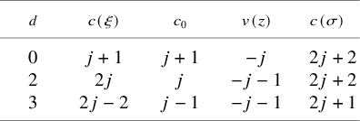
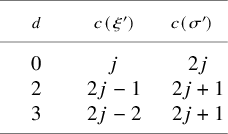
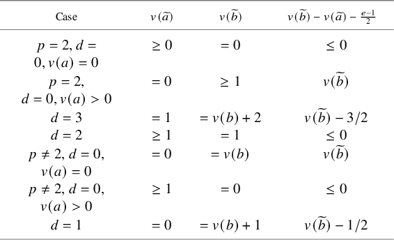


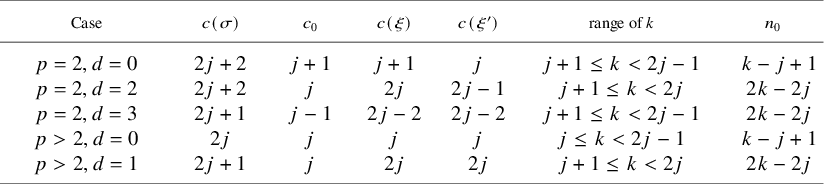

 Open access