1 Introduction
In developmental and educational sciences, researchers often seek advanced methodologies to uncover the intricate relations between variables that shape learning and motivation throughout development (Abacioglu et al., Reference Abacioglu, Isvoranu, Verkuyten, Thijs and Epskamp2019; Li et al., Reference Lee, Tang and Alvarez-Vargas2024; Tang, Lee, et al., Reference Tang, Lee, Wan, Gaspard and Salmela-Aro2022). One such methodology, psychological network analysis (PNA), has emerged as a robust and versatile tool. At its core, psychological network analysis is a statistical method used to explore and visualize the relations among psychological constructs including constructs broadly in social science, treating these constructs as nodes in a network connected by edges that represent associations or dependencies (Borsboom, Deserno, et al., Reference Borsboom, van der Maas, Kievit and Haig2021). Psychological network analysis allows researchers to investigate the complex interplay among psychological constructs, providing a holistic perspective that extends beyond traditional linear models. By visualizing these constructs as interconnected nodes in a network, psychological network analysis offers an intuitive and powerful approach to understanding how individual components interact to form cohesive systems. This Element is dedicated to exploring the theoretical foundations, practical applications, and methodological innovations of psychological network analysis in the context of developmental and educational sciences.
Notably, this Element focuses on psychometric network analysis, a framework used to examine the relations among psychological variables (e.g., symptoms, traits, or beliefs) within individuals or groups. Unlike social network analysis or stochastic actor-oriented models (SOAM), which investigate interpersonal connections between individuals, psychological network models variables as nodes and their statistical associations (e.g., partial correlations) as edges. We therefore distinguish this work from SOAM-type analyses and instead emphasize psychological networks aimed at understanding internal cognitive, emotional, and behavioral processes.
The significance of psychological network analysis lies in its ability to capture the dynamic and multifaceted nature of psychological phenomena. Unlike conventional models that often attribute observed relations to latent variables, psychological network analysis assumes that these relations arise directly from the interplay among observed variables (Abacioglu et al., Reference Abacioglu, Isvoranu, Verkuyten, Thijs and Epskamp2019; Borsboom, Deserno, et al., Reference Borsboom, van der Maas, Kievit and Haig2021). The assumption aligns well with the complexities inherent in developmental and educational research, where constructs such as motivation, cognitive development, and emotional regulation are shaped by a web of interconnected factors. For instance, psychological network analysis can illuminate how factors such as peer relations, teacher support, and emotional well-being interconnect to influence a student’s academic engagement, providing valuable insights for designing interventions that target specific points in these networks (Abacioglu et al., Reference Abacioglu, Isvoranu, Verkuyten, Thijs and Epskamp2019).
The Element opens with a conceptual groundwork for psychological network analysis, introducing its foundational principles, including essential concepts such as nodes and edges, and distinguishing between undirected and directed networks. This section also offers a concise overview of the historical development and current applications of psychological network analysis within developmental and educational sciences, helping readers understand its relevance before engaging in applied procedures.
Building on this foundation, the Element is organized into four major sections, each corresponding to a specific type of data and network construction approach. First, we introduce cross-sectional data, referring to observations collected at a single point in time, typically used to estimate contemporaneous psychological networks.
Second, we focus on cohort data as a form of comparative cross-sectional data drawn from distinct subgroups (e.g., cohorts defined by grade level or age). While methodologically still cross-sectional, cohort data emphasize structured comparisons across naturally occurring subgroups, enabling insights into how network structures may vary across different contexts or populations. We highlight this as a specific application of cross-sectional designs aimed at contextualizing psychological phenomena.
Third, we focus on longitudinal data, where the same individuals are tracked across multiple time points, allowing for the modeling of intra-individual change and temporal dynamics. Fourth, we introduce directed acyclic graphs as a tool for causal inference – structured models that represent directional, non-recursive relations between variables, thus supporting the development and testing of theoretically grounded causal hypotheses.
Each of these four sections includes a detailed, step-by-step guide covering data preparation, network estimation, and interpretation, complemented by practical R code examples. The Element concludes with a dedicated discussion section, in which we synthesize key insights, reflect on the methodological strengths and limitations of psychological network analysis, and outline directions for future research and application.
In short, readers will possess a comprehensive understanding of psychological network analysis, from its theoretical underpinnings to its practical applications. They will be equipped not only to construct and interpret psychological networks but also to critically evaluate their use in research. As psychological network analysis continues to evolve, its integration into developmental and educational sciences can help deepen our understanding of the complex systems that underpin human growth and learning.
2 Theoretical Foundations and Literature Review
2.1 Philosophical Assumptions and Conceptual Foundations of Psychological Network Analysis
2.1.1 Definition and Core Features of Psychological Network Analysis
Psychological network analysis is an analytical framework that conceptualizes psychological phenomena as systems of directly interacting variables (Borsboom, Deserno, et al., Reference Borsboom, van der Maas, Kievit and Haig2021; Epskamp, Waldorp, et al., Reference Epskamp, Waldorp, Mõttus and Borsboom2018). Its core objective is to examine how observed components – such as emotions, behaviors, or beliefs – co-activate and co-regulate within a structured network, without assuming the presence of unobserved latent causes.
Furthermore, psychological network analysis marks a departure from traditional latent variable models, such as factor analysis or structural equation modeling (Epskamp, Rhemtulla, et al., Reference Epskamp, Rhemtulla and Borsboom2017), which posit that shared variance among observed variables is due to underlying constructs. Psychological network analysis treats each observed variable as an active element that may influence and be influenced by others, thereby shifting the analytical focus from inference about hidden traits to the structural configuration of observable interactions (Beard et al., Reference Beard, Millner and Forgeard2016; Borsboom, Deserno, et al., Reference Borsboom, van der Maas, Kievit and Haig2021). As such, one can think of psychological phenomena not as the output of a single hidden mechanism, but as emergent outcomes arising from the mutual activation of system components. For example, an emotional state such as test anxiety may not stem from a single source, but from the reinforcing interactions among worry, physiological arousal, and self-doubt. This interactional view is what psychological network analysis seeks to model and make visible.
2.1.2 Key Concepts: Nodes and Edges
The foundational structure of any psychological network is defined by two primary components: nodes and edges (Epskamp et al., Reference Epskamp, Cramer and Waldorp2012). In most applications, nodes represent observed psychological variables such as emotional states, cognitive beliefs, or behavioral indicators. For instance, in a network modeling anxiety, nodes might include “worry,” “fatigue,” and “sleep disturbance.”
Edges represent the statistical relations between nodes and are typically estimated using partial correlations (Borsboom, Deserno, et al., Reference Borsboom, Deserno and Rhemtulla2021; Epskamp, Maris, et al., Reference Epskamp, Rhemtulla and Borsboom2017). These edges convey the unique association between two variables after accounting for all others in the network (Borsboom, Deserno, et al., Reference Borsboom, van der Maas, Kievit and Haig2021; Epskamp, Maris, et al., Reference Epskamp, Rhemtulla and Borsboom2017). The edges are often weighted, with their thickness corresponding to the strength of the connection between the nodes, and the presence or absence of edges helps define the structural configuration of the psychological system. In some cases, edges may be directional, indicating a temporal or hypothesized causal influence.
2.1.3 Rationale for Adopting a Network Perspective
The network perspective is particularly well suited to developmental and educational psychology, where psychological processes are often embedded in complex, dynamic systems, and cannot be adequately addressed through a single, linear perspective (Hastie et al., Reference Hastie, Tibshirani, Wainwright, Hastie, Tibshirani and Wainwright2015; Tang, Lee, et al., Reference Tang, Lee, Wan, Gaspard and Salmela-Aro2022). These systems span cognitive, emotional, social, and contextual dimensions, and their components tend to interact in non-linear and mutually reinforcing ways (Donelli & Matas, Reference Donelli and Matas2020; Neal & Neal, Reference Molenaar and Nesselroade2013). Traditional analytic models frequently oversimplify such complexity by emphasizing unidirectional causality or assuming static structures (Tang, Reference Swendsen, Tennen and Carney2020).
Additionally, psychological network analysis aligns with theoretical perspectives that emphasize system-level interdependence, temporal change, and context sensitivity (Epskamp, Maris, et al., Reference Epskamp, Rhemtulla and Borsboom2017). These include dynamic systems theory and ecological approaches, which argue that psychological development results from recursive interactions within and between levels of functioning – ranging from individual cognition to broader social environments (Martin & Lazendic, Reference Li and Kwok2018).
Importantly, the visual representation of a network adds further depth to the analysis (Jones et al., Reference Jones2018). The edges are often weighted, with their thickness corresponding to the strength of the connection between the nodes. By visualizing the intensity and structure of these relations, networks enable researchers to identify entire systems of interaction rather than isolated variables (Cui et al., Reference Cui, Yang and Gao2022; Ren et al., Reference Peng, Yuan and Wei2021). This approach allows for a more nuanced understanding of psychological phenomena, emphasizing how variables collectively contribute to complex behaviors and outcomes, rather than treating them as isolated factors.
Consider anxiety as an illustrative example. From a network perspective, anxiety is not the product of a latent disposition but the emergent outcome of reciprocal interactions among symptoms such as worry, restlessness, and sleep disturbance. In educational settings, a similar logic applies to motivational dynamics: Factors such as perceived academic pressure, self-efficacy, and task avoidance can interact to create feedback loops that either support or undermine engagement. Psychological network analysis provides the methodological tools to capture and explore these complex interrelations over time and across contexts.
2.1.4 Network Types in Psychological Research
Psychological networks can be classified in various ways depending on their structure, statistical properties, and research purposes. One of the most fundamental distinctions is based on whether the edges are directional or not, dividing network models into two broad categories: undirected networks and directed networks. This classification not only reflects the theoretical interpretation of the relations between variables but also determines the type of data required and the estimation procedures employed (Borsboom, Deserno, et al., Reference Borsboom, van der Maas, Kievit and Haig2021; Panayiotou et al., Reference Neal and Neal2023).
In undirected networks, edges are symmetrical and represent mutual associations between variables. Most commonly, these associations are quantified using partial correlations, indicating the unique relation between two nodes while controlling for all others in the network. Undirected networks are particularly useful for exploring the structure of cross-sectional or cohort data, allowing researchers to identify core variables, detect tightly connected clusters, and investigate the organization of psychological constructs.
In contrast, directed networks include edges with a specified direction, reflecting hypotheses about temporal ordering or causal influence. These models are typically applied to longitudinal or intensive time series data and provide tools for investigating the dynamic evolution of psychological processes and for exploring potential causal pathways among variables.
In conclusion, the type of network model selected should align with both the research question and the nature of the available data. The following sections provide a more detailed discussion of undirected and directed networks, including theoretical foundations, estimation techniques, and illustrative applications in developmental and educational psychology.
2.2 Undirected Psychological Networks
Undirected networks are widely used for exploring the structural organization of psychological constructs based on cross-sectional or cohort data. The process of constructing an undirected network typically begins with variable selection, where researchers identify relevant variables based on theoretical or empirical considerations. This is followed by fitting a network model, where partial correlations between variables are computed (Burger et al., Reference Burger, Isvoranu and Lunansky2023). Once the network is fitted, its accuracy and stability are assessed through methods like bootstrapping to evaluate edge weights and centrality measures (Epskamp, Borsboom, et al., Reference Epskamp, Borsboom and Fried2018). Finally, researchers interpret the network, focusing on significant edges, central nodes, and clusters that represent closely connected constructs.
2.2.1 Modeling Cross-Sectional Data
Cross-sectional data capture observations at a single time point and are widely used to examine how psychological variables co-occur across individuals. Undirected networks are particularly suited to such data, as they model bidirectional associations – typically partial correlations – without making assumptions about causality or temporal ordering. These networks feature bidirectional edges, indicating mutual associations (Epskamp & Fried, Reference Epskamp and Fried2018).
Such networks are invaluable for identifying interrelated variables, providing insights into their latent interactions. For instance, a study on multicultural classroom dynamics mapped out the interplay between teachers’ multicultural approaches, peer relations, and student motivation in primary school classrooms (Abacioglu et al., Reference Abacioglu, Isvoranu, Verkuyten, Thijs and Epskamp2019). Another undirected network study used two types of networks (correlation-based network analysis and co-occurrence network analysis) to discover the key differences between curiosity and interest among the net of many other motivations and emotions (Tang, Renninger, et al., Reference Tang, Lee, Wan, Gaspard and Salmela-Aro2022).
2.2.2 Applications to Cohort- and Group-Level Data
Although undirected networks based on cross-sectional data are effective for exploring the structure of psychological constructs, they are inherently limited in capturing developmental change or group-based variability. Because all observations are treated as coming from a single homogeneous sample, structural differences between subgroups – such as those based on age or educational level – are often masked or averaged out.
Cohort data offer a useful extension. These data involve distinct subgroups (or cohorts) that differ systematically by characteristics such as grade, age, gender, or institutional background. Although cohort designs do not track the same individuals over time, they allow researchers to approximate developmental patterns and compare network structures across groups in a controlled manner.
Furthermore, network analysis with cohort data typically involves estimating separate networks for each group and comparing their structural features. Researchers may examine whether key variables shift in centrality across cohorts, whether edge strengths are preserved or altered, and whether overall network density or modularity changes with developmental stage. Statistical tools such as the Network Comparison Test (NCT) can be used to formally assess these differences. For instance, one might compare student motivation networks across age-based cohorts within a school setting. Younger groups may display more densely interconnected emotional and cognitive variables, reflecting integrated motivational patterns, whereas older cohorts tend to exhibit more differentiated and functionally specialized structures. These comparisons provide insight into the developmental progression of psychological constructs and support the design of age-appropriate interventions in educational and mental health contexts.
2.3 Directed Psychological Networks
Unlike undirected networks, which represent mutual associations between variables, directed networks encode the direction of influence – allowing researchers to examine how one variable may affect another. These models are especially valuable when exploring psychological processes that unfold over time or follow hypothesized causal pathways (Borsboom, Deserno, et al., Reference Borsboom, Deserno and Rhemtulla2021; Epskamp, Waldorp, et al., Reference Epskamp, Waldorp, Mõttus and Borsboom2018).
Directed networks support more dynamic and explanatory modeling than their undirected counterparts. In psychological research, they are typically implemented in two forms. The first uses longitudinal or time series data to estimate time-lagged effects. The second adopts a directed acyclic graph approach to infer potential causal structures based on conditional independence. The following sections introduce these two modeling strategies and illustrate their application in developmental and educational contexts.
2.3.1 Longitudinal Network Models
Different from static cross-sectional networks, which provide a snapshot of associations at a single time point, longitudinal networks provide a framework for examining how psychological variables influence one another across time, and allow researchers to study processes that unfold across multiple time points, offering deeper insights into changes and interactions within developmental and educational contexts (Borsboom, Deserno, et al., Reference Borsboom, Deserno and Rhemtulla2021; Epskamp, Waldorp, et al., Reference Epskamp, Waldorp, Mõttus and Borsboom2018).
Longitudinal network modeling typically yields three complementary types of networks, each capturing a distinct layer of temporal dynamics and offering unique interpretive value. In each network, the meaning of an edge – whether it reflects direction, timing, or population-level association – must be interpreted with reference to the underlying data structure.
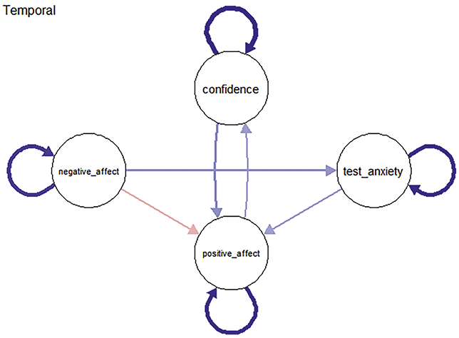
Temporal networks are directed and model lagged relations between variables across successive time points (e.g., from time t−1 to time t), controlling for all variables at the earlier time point. Edges in temporal networks reflect the lagged associations among variables. These lagged associations are commonly interpreted using the logic of Granger causality (Granger, Reference Granger1969), which suggests that if the past state of one variable improves the prediction of another variable’s future state, then the first variable can be said to Granger-cause the second. This does not imply true causal influence but rather statistical precedence and prediction. Temporal networks are thus particularly useful for examining how psychological states may activate, sustain, or regulate one another over time. To some extent, they can also reflect potential causal dependencies between variables. Importantly, self-directed edges (autoregressive edges) – arrows pointing from a variable to itself across time – represent the variable’s own stability or inertia over time (e.g., persistent levels of anxiety or self-efficacy).
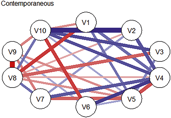
Contemporaneous networks are undirected and capture associations among variables within the same time point, after accounting for lagged effects. Edges in these networks reflect momentary changes not explained by temporal effects or changes occurring faster than the specified lag (Jordan et al., Reference Jones, Mair and McNally2020). In other words, edges represent partial correlations among residuals at each time slice, highlighting how variables co-activate instantaneously or interact within the same moment. These networks do not imply directionality or predictive influence, but instead reflect symmetric, momentary dependencies among variables.
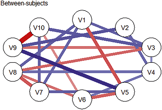
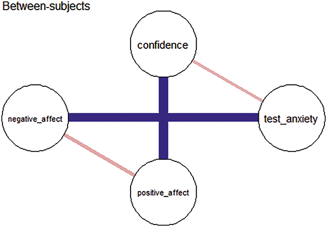
Between-subjects networks depict the average associations among mean variable levels across participants and time points, and provide insights into how trait-like variables tend to co-occur at the population level, independent of temporal order. That is, between-subjects network captures how variables covary in terms of their average levels, which corresponds to what is known as the variance-covariance structure (Epskamp, Waldorp, et al., Reference Epskamp, Waldorp, Mõttus and Borsboom2018). Because this structure is often used in traditional cross-sectional studies to describe relations between variables, the between-subjects network could serve as a useful bridge – allowing researchers to meaningfully compare findings from longitudinal data with results from prior cross-sectional research (Epskamp, van Borkulo, et al., Reference Epskamp, van Borkulo and van der Veen2018; Epskamp, Waldorp, et al., Reference Epskamp, Waldorp, Mõttus and Borsboom2018).
Longitudinal network analysis commonly relies on longitudinal data, which can broadly be categorized into two common types: panel data and time series data. Panel data involves repeated measurements from multiple individuals over a limited number of time points (N > T). This data type characterizes both the association structure of variables at a given time point and how these conditional dependencies change over time, which makes them especially suitable for studying developmental changes and interindividual variability simultaneously. For example, Panayiotou et al. (Reference Neal and Neal2023) conducted a network analysis of adolescent mental health using panel data collected across five time points over ten years from thousands of participants. The study identified strong autoregressive effects, indicating temporal stability in key symptoms, and revealed that increased social media use among female participants was associated with greater concentration over time, which, as a component of mental health, can reflect aspects like attention difficulties or cognitive load. Similarly, Speyer et al. (Reference Smith and Juarascio2022) analyzed socio-emotional development using panel data from children (ages 4–9) and adolescents (ages 11–16) across multiple developmental stages. By comparing longitudinal networks across age groups, the study uncovered distinct temporal association patterns within each group. For instance, the adolescent network exhibited a greater number of stronger connections compared to the childhood network. In contrast, the childhood network showed more prominent self-regressive (autoregressive) effects, which were less evident in adolescents. These findings illustrate how the structure of socio-emotional traits changes over time and reflect the distinctive developmental characteristics of each stage.
In contrast, time series data also involves repeated measurements, but is characterized by more intensive time points (T=large) and can focus on a single individual or multiple persons assessed intra-individually (N >= 1). This type of data primarily focuses on capturing dynamic changes within an entity, such as daily mood ratings for one person. Networks derived from time series data are most often applied in situations where one seeks insight into the dynamic structure of systems. For instance, Peng et al. (Reference Pearl and Verma2024) collected daily reports of eight generalized anxiety disorder symptoms from 115 participants over 50 days, and the analysis identified positive lagged relations and autocorrelations among symptoms.
Importantly, longitudinal network models are particularly suited for exploring potential causal pathways among psychological variables. By encoding directional edges, these models move beyond descriptive associations to hypothesize how one variable may influence another. This capacity makes them especially valuable in educational and mental health research, where understanding the mechanisms underlying change is often central (Lee et al., Reference Larson2024). For instance, Fried et al.(Reference Fried, Papanikolaou and Epskamp2022) used ecological momentary assessment with intensive temporal data during the COVID-19 pandemic to uncover a maladaptive cycle in undergraduate mental health: Alone → COVID-19-worry → COVID-19-preoccupation → Anhedonia ⇄ (worry about) Future ⇄ Alone. This directed network revealed how affective and cognitive symptoms may sustain one another, offering valuable insights for prevention and intervention.
Longitudinal network models are also effective in contexts where prior theoretical guidance is limited and relations between variables are not yet well understood. In these cases, exploratory longitudinal network analysis provides a data-driven approach to uncovering candidate causal structures (Borsboom, Deserno, et al., Reference Borsboom, Deserno and Rhemtulla2021; Haslbeck et al., Reference Haslbeck, Ryan, Robinaugh, Waldorp and Borsboom2021). For example, a longitudinal psychological network study examined the development of PTSD symptoms and their functional consequences among UK healthcare workers during the COVID-19 pandemic (Freichel et al., Reference Freichel, Herzog and Billings2024). Based on data collected over seven time points, the analysis revealed a mutually reinforcing pattern between intrusion and avoidance symptoms, with intrusion emerging as a particularly influential symptom that contributed to downstream functional impairments, such as difficulties in performing work-related tasks.
2.3.2 Directed Acyclic Graphs
Directed acyclic graphs are graphical models used to represent and explore potential causal relations between variables (Epskamp, Waldorp, et al., Reference Epskamp, Waldorp, Mõttus and Borsboom2018). Directed acyclic graphs are also directed networks, in where each node denotes an observed or latent variable (e.g., “test anxiety,” “academic performance”), and each directed edge (an arrow) indicates a hypothesized causal influence from one variable to another. The term “acyclic” refers to the absence of cycles, meaning that a variable cannot eventually cause itself through a feedback loop. This ensures that causal pathways flow in one direction, forming a coherent hierarchy of influence. For example, consider a model in which test anxiety leads to reduced working memory capacity, which in turn affects problem-solving accuracy. A corresponding directed acyclic graph might represent this as: Anxiety → Working Memory → Accuracy, clarifying the chain of causal influence and identifying possible mediators.
2.3.2.1 Theoretical Foundation and Directed Acyclic Graph Construction
The core ideas behind directed acyclic graph are to make statistical causal inferences given the changes of networks among variables. This process begins with identifying conditional associations between variables. In the section on cross-sectional data, we introduced that network analyses establish links between nodes by controlling for all other variables. These links could be understood as partial correlations, which reveal variable relations under controlled conditions (Borsboom, van der Maas, et al., Reference Borsboom, van der Maas, Kievit and Haig2021; Epskamp, Waldorp, et al., Reference Epskamp, Waldorp, Mõttus and Borsboom2018). In contrast, another type of correlation network involves zero-order correlations (often calculated using Pearson’s correlation coefficient). These reflect the direct association between two variables without accounting for other factors. Put differently, relations in partial correlation networks represent the net connection between two nodes after controlling for others, whereas relations in zero-order correlation networks reflect the total association, which doesn’t exclude the influence of common causes, mediating variables, or mere covariation without direct causality.
Building on this, if there are discrepancies in edges between zero-order and partial correlation networks – for example, an edge present in the zero-order network but absent in the partial correlation network – we can infer that this discrepancy arises because, after controlling for other nodes, a key node is associated with both nodes forming the edge, thereby causing the edge to disappear. By systematically examining sub-partial correlation networks of three nodes and iterating through the entire network, we can identify this critical node. For instance, consider a scenario where the relation between variables “B” and “C” exists in the zero-order network but vanishes in the partial correlation network. If we observe that “B” and “C” maintain their connection in partial correlation networks with other nodes, but their association disappears specifically when forming a network with “A,” then it’s highly probable that “A” has a potential association with B (or C), thereby influencing the B-C relation.
Directed acyclic graph algorithms take this a step further by identifying the minimal set of directed connections that best explain the observed dependencies while preserving acyclicity. Estimation algorithms use these patterns to determine which edges are necessary to explain the observed relations and in which direction they should point. A representative method for this is the Inferred-Causation Algorithm (ICA; Pearl, Reference Panayiotou, Black, Carmichael-Murphy, Qualter and Humphrey1988; Pearl & Verma, Reference Pearl1995). For example, if introducing variable “A” causes the correlation between variables “B” and “C” to vanish, this suggests an inverted fork causal structure (B → A ← C), where “A” serves as the collider (Rohrer, Reference Robinaugh, Millner and McNally2018). In other words, in a partial correlation network comprising nodes “B,” “C,” and other variables (excluding “A”), the association between B and C will appear because “A,” as the collider, isn’t accounted for and thus has no conditioning effect. However, when “A” is included in the partial correlation network with B and C, their association vanishes because A’s influence is now considered. Thus, the directional relations among nodes “A,” “B,” and “C” become explicit after ICA.
The results of network analysis, thus, can lay the foundation to construct directed acyclic graphs while using the ICA algorithm. In corresponding sections, we will present concrete examples illustrating how to use network analysis to derive directed acyclic graphs, offering a complete guide from theoretical foundations to practical application.
2.3.2.2 Relation to Undirected and Longitudinal Network Approaches
The construction of directed acyclic graphs is closely related to, but distinct from, undirected psychological networks. Though undirected networks are exploratory tools for visualizing the structure of associations, directed acyclic graphs impose a more interpretive framework: They aim to uncover which variables might causally influence others. Directed acyclic graph learning builds upon the skeleton of undirected networks (e.g., conditionally dependent edges) but adds assumptions about causal sufficiency and the absence of unmeasured confounding to justify the inferred directions.
Additionally, it is important to note that directed acyclic graphs differ significantly from traditional directed networks, such as temporal networks based on longitudinal data. First, in most cases, directed acyclic graphs are not bound to time-indexed data and instead use statistical structure to identify directional paths. This makes them particularly valuable in research contexts where longitudinal data are unavailable or experimental manipulation is infeasible. Then, temporal networks typically include autoregressive edges (e.g., self → self across time), which are absent in directed acyclic graphs due to the acyclic constraint. Moreover, temporal networks assume a known data ordering (time), whereas directed acyclic graphs can infer causal ordering from cross-sectional data – often when no temporal information is available. In this sense, directed acyclic graphs serve as an algorithmic counterpart to both undirected and directed networks, bridging exploratory association mapping and causal modeling.
2.3.2.3 The Role of Directed Acyclic Graphs in Psychological and Educational Causal Modeling
Traditional methods of causal inference – such as randomized controlled trials or longitudinal path models – are often difficult to implement in real-world educational and developmental settings. Constraints on time, ethics, and control make it challenging to manipulate key psychological variables experimentally. Similarly, though time-based network models offer insights into temporal dynamics, they require intensive repeated measurement and are sensitive to time window selection and missingness.
Directed acyclic graphs offer a practical alternative by enabling researchers to derive plausible causal hypotheses from observational data. In developmental psychology, directed acyclic graphs can help illuminate how constructs such as self-regulation, emotion, and learning behavior interact hierarchically. In education, they can model how different psychological and contextual factors jointly influence academic outcomes – for example, Motivation → Learning Strategy Use → Academic Performance, helping inform intervention strategies.
Crucially, directed acyclic graphs do not claim to prove causality. Instead, they provide a transparent, assumption-driven framework for articulating and testing causal hypotheses. By identifying testable pathways and controlling for potential confounders through structure learning, directed acyclic graphs support theory development, particularly in domains where empirical evidence is rich but theoretical consensus is limited.
3 Psychological Network Analysis with Cross-sectional Data
3.1 Overview
In previous sections, we introduced undirected psychological networks as tools for modeling the structure of associations among observed variables. In these networks, nodes represent psychological constructs or behaviors, and edges reflect the conditional associations between them, typically estimated as partial correlations that account for the influence of all other variables in the system. This modeling approach allows researchers to explore the configurational patterns of psychological phenomena, identify co-activated variables, and develop theory-driven insights. Because of their intuitive graphical form and data-driven logic, undirected networks have become a valuable tool for exploratory research in developmental and educational science.
Nevertheless, fitting a single network model to a dataset often produces only a static and surface-level representation of the underlying psychological structure. In many real-world applications, researchers are interested not only in the presence of connections but also in identifying which variables play particularly influential roles, or in understanding how the structure of relations may shift across different groups or contexts. To address such analytical needs, psychological network analysis can be extended through two complementary techniques: centrality analysis and network comparison analysis, both of which enable deeper insights into the function and variability of psychological systems (van Borkulo et al., Reference Thissen, Steinberg and Kuang2023).
Centrality analysis focuses on determining the importance of each node in the network from multiple perspectives. For instance, strength centrality quantifies how strongly a variable is directly connected to other variables by summing the absolute values of its edge weights, offering a sense of its overall connectivity. Closeness centrality evaluates how efficiently a variable can access the rest of the network, based on the length of shortest paths. Meanwhile, betweenness centrality indicates how often a variable acts as a bridge linking otherwise disconnected parts of the system. These indices allow researchers to identify core psychological constructs that may organize the system, drive change, or serve as optimal targets for intervention.
Network comparison analysis provides a structured approach to examining how psychological networks differ across groups or conditions. It typically involves three main aspects. The first is structural edge differences, which refer to whether specific connections between variables are present in one network but not in another. This allows researchers to identify differences in the functional relations between variables across various groups, such as variations in the strength or presence of connections between a given pair of variables. The second is edge strength differences, which examine whether the magnitude of these connections – represented by edge weights – differs for the same variable pairs across networks, revealing which relations become stronger or weaker under different conditions. The third is global strength, which compares the total level of connectivity across networks and helps evaluate whether one system is more cohesive or diffuse than another. Together, these complementary dimensions offer a clear and multifaceted way to understand how network structures vary, and why such differences might matter in developmental or educational contexts.
In this section, we will provide guidance on conducting psychological network analysis when examining relations among variables in cross-sectional data. This section will be organized into two main parts. The first part will cover the general steps of cross-sectional psychological network analysis, including sample collection, variable selection, network estimation, centrality analysis, and edge accuracy testing. The second part will introduce specific analytical methods for particular research needs, such as further interpretation of centrality indices and group comparisons of network structures, adding depth to the analysis.
To ensure practical applicability, this section will provide complete R code examples, covering the necessary R packages (e.g., psych, qgraph, and bootnet) and relevant functions. With these examples, readers can fully replicate the steps of psychological network analysis in the R environment, gaining a clear understanding of the purpose and methods behind each analytical process. All the codes and supplementary materials can also be accessed at https://osf.io/5n6v8/.
3.2 Step-by-Step Tutorial
3.2.1 Steps Overview
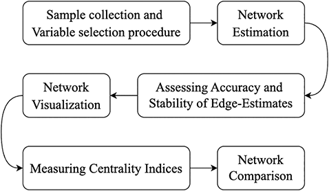
In psychological network analysis, there are several key steps, as shown in Figure 1: sample collection, variable selection, network estimation, accuracy and stability analysis, and network visualization and interpretation (Burger et al., Reference Burger, Isvoranu and Lunansky2023). Sample collection and description serve as the starting point of the analysis, ensuring that the data is representative and robust. Variable selection and measurement determine the interpretability of the model, ensuring that it accurately reflects the psychological traits or constructs being studied. The choice and application of network estimation methods allow for the construction of a graph that represents associations between variables (Epskamp & Fried, Reference Epskamp and Fried2018). Accuracy and stability testing of edge weights ensure the robustness and reliability of the model (Epskamp, Borsboom, et al., Reference Epskamp, Borsboom and Fried2018). Finally, network visualization and interpretation enable researchers to intuitively display complex relational networks, providing visual support for identifying key nodes and edges within the network (Jones et al., Reference Jones2018). Together, these steps form a solid analytical workflow, guiding the process from data preparation to model construction and result presentation, each step contributing crucially to building and interpreting the network model.
The analysis process of undirected networks

3.2.2 Step 1: Sample Collection and Variable Selection Procedure
Sample collection is the starting point of psychological network analysis and should include information on data sources, participant characteristics (e.g., sample size, gender, age), and methods for data collection and selection.
Variable selection is a critical step in psychological network analysis. As in other educational psychology and developmental studies, it is essential to accurately report the tools or methods used for data collection. This involves clearly specifying which measurement instruments were used (e.g., questionnaires, interviews, or observations) and how each variable was measured by these instruments. Additionally, a detailed description of data processing is necessary, such as whether scores were transformed, missing values handled, or variables standardized. This information helps ensure research transparency, allowing readers to understand the source and treatment of the data, thereby enabling a more accurate evaluation of the study’s reliability.
Example
In this example, we use the bfi dataset from the psych package. This dataset includes Big Five personality trait assessment data from 2,800 participants, with 25 self-assessment items corresponding to the 5 personality traits: agreeableness, conscientiousness, extraversion, neuroticism, and openness. Additionally, it contains three demographic variables: gender, education level, and age. The research questions we will examine include: “What is the relation between education level, age, and personality traits?” and “Do the mechanisms of influence for these personality traits differ significantly between young adults (ages 18–31) and middle-aged adults (ages 31–60)?”
We use the tidyverse package to calculate summary scores for each Big Five personality dimension from the bfi dataset. Additionally, we include two demographic variables: education level and age. Participants were selected and divided into two groups based on their age: young adults (18–30 years old) and middle-aged adults (31–60 years old). This grouping allows us to explore how developmental differences shape the relations among the Big Five personality traits.
library(tidyverse)library(psych)data(bfi) # Load the psych package and bfi datasetstr(bfi) # View the basic structure of the datasetsummary(bfi) # Briefly summarize the dataset variables and information# Generate total datasetbfi_sum <- bfi |> transform( A = A1+A2+A4+A4+A5, C = C1+C2+C3+C4+C5, E = E1+E2+E3+E4+E5, N = N1+N2+N3+N4+N5, O = O1+O2+O3+O4+O5) |>select (A, C, E, N, O, education, age)
3.2.3 Step 2: Network Estimation
There are several multivariate models available for constructing psychological networks, which estimate edge weights and visualize network structures (Epskamp, Borsboom, et al., Reference Epskamp, Borsboom and Fried2018; Epskamp, Waldorp, et al., Reference Epskamp, Waldorp, Mõttus and Borsboom2018). In this Element, we focus on a specific type of network model – the Pairwise Markov Random Field (PMRF) – to construct psychological networks (Epskamp & Fried, Reference Epskamp and Fried2018). This undirected model represents variables as nodes and conditional association strengths between pairs of variables as edges, controlled for all other variables in the network. PMRF includes three main subtypes:
1. Ising Model: This model is suitable for binary data (Epskamp, Maris, et al., Reference Epskamp, Maris, Waldorp and Borsboom2017; Ernst, Reference Ernst1925; Waldorp et al., Reference van Geert and Steenbeek2019) and commonly used to analyze associations in binary variables, such as yes/no responses.
2. Gaussian Graphical Model (GGM): Designed for continuous data (Epskamp, Maris, et al., Reference Epskamp, Maris, Waldorp and Borsboom2017), GGM is the standard model for conditional independence among continuous variables and is widely used in educational psychology to examine linear associations.
3. Mixed Graphical Model (MGM): This model handles mixed data types, including continuous, categorical, and count data (Haslbeck & Waldorp, Reference Haslbeck and Waldorp2015), making it ideal for educational psychology studies with diverse variable types.
Like other models used in developmental and educational research, psychological network models are essentially multivariate statistical models. Therefore, estimating model parameters (i.e., edge weights in the network) involves choosing an appropriate estimation method (Isvoranu & Epskamp, 2023). Various model selection algorithms are available to identify the most relevant edges, creating an optimal network structure. However, there is no single “best” algorithm, as the choice often depends on sample size and variable count, making a careful algorithm selection essential.
Each model selection algorithm has its own characteristics. Some algorithms are highly sensitive and retain a large number of connections between variables, resulting in a dense network, a structure where most nodes are interconnected and many associations are preserved. Others are more conservative, omitting edges that are statistically insignificant, meaning their estimated strength is not reliably different from zero when accounting for sampling variability. Some algorithms also exclude edges that are non-standard-compliant, referring to connections that violate theoretical assumptions or mathematical constraints required by the model, such as symmetry, acyclicity, or positive definiteness. In addition, certain algorithms provide more stable and interpretable parameter estimates, which refer to the quantified relations (e.g., edge weights) between variables in the network. This often leads to simpler and more robust models that are easier to understand and apply.
Here, we introduce four common model selection algorithms:
1. Thresholding begins with a saturated network – a structure in which all possible connections between variables are initially included – and removes edges with weak statistical support or those that conflict with structural assumptions, resulting in a clearer and more focused network.
2. Pruning involves explicitly setting some edges to zero based on predefined rules, followed by re-estimation of the network with the remaining connections. This helps strike a balance between complexity and parsimony.
3. Model-search scans across the space of possible network configurations, ranging from simple independence models (where no edges are assumed) to fully connected saturated models, in order to identify the best-fitting structure.
4. Regularization introduces penalty terms into the estimation process that gradually shrink weak edge weights toward zero, which often used in machine learning. This results in a sparse network, meaning one that contains only the most stable and essential connections, and is typically more generalizable, or better able to reproduce consistent results in new datasets.
In summary, selecting an appropriate algorithm depends on the data characteristics and specific research question. Although this section does not delve deeply into each algorithm’s technical details, we recommend resources for readers to explore the distinct features, applicable contexts, and supported software or R packages for each method.
Example
In this section, we use the bootnet package to fit network models. bootnet is a powerful R package designed for estimating and validating psychological networks. It provides a versatile framework that simplifies network analysis by utilizing network estimation algorithms implemented in other R packages. In this example, we employ the estimateNetwork() function from bootnet, with the parameter default = “EBICglasso.” The EBICglasso method (Extended Bayesian Information Criterion Graphical LASSO) is a widely used regularization technique that generates a sparse and stable network model by shrinking edge weights, making it ideal for high-dimensional data. This method controls the number of edges, improving the network’s interpretability and visualization.
# fit the network model to the total samplelibrary(bootnet)net_sum<-estimateNetwork(bfi_sum,default = "EBICglasso",threshold = TRUE)
3.2.4 Step 3: Assessing Accuracy and Stability of Edge-Estimates
In psychological network analysis, the accuracy of edge weights and the stability of the network structure are essential for assessing model quality. Accuracy refers to the precision of the edge weight estimates. Meanwhile, stability indicates whether the network structure remains consistent under various sampling conditions. Testing these aspects helps ensure the reliability of the model results, allowing for confident interpretation of key edges and nodes within the network.
The bootnet package provides several methods for robustness testing. For accuracy, bootnet uses confidence intervals around the edge weights, computed through nonparametric bootstrapping. This involves repeatedly resampling to create confidence intervals for each edge weight. Narrow confidence intervals indicate more reliable edge estimates, whereas wider intervals suggest that an edge may be less stable and should be interpreted cautiously.
For stability, bootnet offers resampling-based stability tests. One common approach is case-drop bootstrap stability testing, which examines whether the network structure holds when portions of the data are removed. By gradually omitting a certain percentage of the data and re-estimating the network, researchers can observe whether measures such as edge strength change significantly, providing insight into the consistency of the network’s key elements.
Example
We use the accuracy and stability testing methods provided in the bootnet package to evaluate network results. First, we apply nonparametric bootstrapping to estimate the precision of edge weights, computing 95 percent confidence intervals for all edge weights by resampling 5,000 times. Narrow confidence intervals indicate higher accuracy of network estimates (Epskamp, Borsboom, et al., Reference Epskamp and Fried2018). For stability, bootnet employs the m out of n bootstrap method, removing a proportion of cases to generate new samples. If the centrality rankings in the original network closely match those in the resampled networks, it indicates good network stability (Epskamp, Borsboom, et al., Reference Epskamp, Borsboom and Fried2018).
In bootnet, both accuracy and stability checks are performed using the bootnet function. However, for stability testing, we set the type parameter to “case” to apply the case-drop bootstrap method, removing a portion of the sample in each iteration to assess network stability under varying data conditions. The remaining key parameters in the code are as follows:
1. nBoots = 5000: Specifies the number of bootstrap samples, set to 5,000 here. A higher number of bootstraps help achieve more accurate estimates, especially for edge weight confidence intervals and stability results.
2. nCores = 8: Sets the number of cores for parallel processing to 8, which enhances computational speed in a multi-core environment, significantly reducing runtime for high-frequency bootstrapping.
# Check for accuracy and stability# Calculate Accuracy with bootstrapboot1_sum <- bootnet(net_sum, nBoots = 5000, nCores = 8)# Calculate Stability using bootstrap case methodboot2_sum <- bootnet(net_sum, nBoots = 5000,type = "case",nCores = 8)
After completing edge weight accuracy and network stability tests, the bootnet package generates two essential visual outputs:
On the one hand, Edge Accuracy Plot displays the confidence intervals (typically 95 percent) for each edge, assessing the precision of edge weight estimates. Narrow intervals indicate robust edge estimates, allowing for confident interpretation of their strength; wide intervals suggest instability, warranting cautious interpretation. On the other hand, Network Stability Plot shows changes in centrality indices (e.g., strength, betweenness, closeness) as a proportion of data is removed iteratively. If these measures remain stable despite data variations, it indicates a robust network structure with high reliability.
The code for generating these plots is as follows:
Plot(boot1_sum)Plot(boot2_sum)
3.2.5 Step 4: Network Visualization
In psychological network analysis, network visualization is a crucial step for presenting the relations among variables. A clear network graph visually highlights important nodes and the strength of connections (edges) between them, making the network structure easier to interpret.
The bootnet package provides a plot function for visualizing network estimation results, offering an intuitive display of edge weights and node relations.
# Plot the network for the population sampleplot(net_sum)
3.2.6 Step 5: Measuring Centrality Indices
In addition to the general steps introduced earlier, there are other methods to further investigate the complex relations between variables. Here, we focus on two commonly used methods: centrality indices and network comparison analysis.
Centrality indices measure the importance of nodes within a network and are commonly used in specific analyses to gauge each node’s role in the network. They help identify key variables in the network – those that are highly connected, act as bridges between other nodes, or are closely associated with other variables. The most commonly used centrality indices are strength, betweenness, and closeness, each revealing different aspects of a variable’s potential influence and function within the network (Jones, Reference Isvoranu, Epskamp, Waldorp and Borsboom2023).
1. Strength indicates the total connection strength of each node. Nodes with high strength values are often core variables in the network, demonstrating strong associations with other nodes
2. Betweenness measures a node’s importance within a network by quantifying how often it lies on the shortest path connecting any two other nodes. This directly reflects the node’s capacity to funnel activity or influence, establishing it as a critical bridge controlling the flow of information or variable associations.
3. Closeness indicates how closely a node is connected to all other nodes, revealing nodes with broad influence across the network due to their proximity to other nodes.
Example
To calculate and visualize centrality indices, we can use the centralityPlot function from the qgraph package. This function helps visualize centrality metrics such as strength, closeness, and betweenness, highlighting the relative importance of each node in the network. Key parameters for the centralityPlot function are as follows:
1. scale sets the scale for the x-axis. Options include “z-scores” to standardize centrality values, “raw” to show original centrality values, “raw0” to include zero on the x-axis, and “relative” to standardize values on a 0-to-1 scale for easier comparison.
2. relative is a logical argument controlling whether to rescale all metrics relative to the maximum value.
3. include specifies which centrality metrics to calculate and display, such as strength, closeness, and betweenness. The default includes all available centrality metrics, or set to “all” to include all.
# Load the qgraph packagelibrary(qgraph)centralityPlot(net_sum, include=c("Strength","Closeness", "Betweenness"), scale = "raw", relative = TRUE)+labs(title = "net of total sample")
3.2.7 Step 6: Network Comparison
Network comparison is used to analyze differences in psychological network structures between pre-defined groups (e.g., gender, age, or cultural background). This process enables researchers to explore whether the way variables are associated differs across populations, uncovering meaningful group-specific patterns. Three main aspects are typically tested:
1. Network structure invariance examines whether the pattern of connections – that is, which pairs of variables are connected by an edge – remains the same across groups. A significant result indicates that some edges are present in one group’s network but not in the other, suggesting structural variation in the psychological system.
2. Global strength invariance tests whether the overall connectivity level of the network differs between groups. This is usually quantified by summing the absolute edge weights of all connections in each network, yielding a measure known as global strength. A difference in global strength suggests that one group has a more densely connected or integrated psychological profile than the other.
3. Edge invariance focuses on individual connections and evaluates whether the weight of specific edges (i.e., the strength of association between two variables, controlling for others) significantly differs across groups. This helps identify which relations are uniquely stronger or weaker in one group relative to another.
In R, the NetworkComparisonTest package’s NCT function can be used for this purpose (van Borkulo et al., Reference Thissen, Steinberg and Kuang2023).
Example
In this section, we selected two groups from the overall dataset: early adults (ages 18–30) and middle-aged adults (ages 31–60). By analyzing the psychological network fitting results for these two groups, we aim to explore whether there are significant differences across age stages and further uncover the potential mechanisms through which age influences the Big Five personality traits. To compare the networks of these two groups, it is necessary to conduct the standard steps of psychological network analysis for each subgroup, including dataset splitting, network estimation, and accuracy and stability testing. However, due to space constraints, this section will focus solely on presenting the results of the network comparison.
We use the NCT function from the NetworkComparisonTest package to compare the overall structure, edge strength differences, and global network strength between two networks. Key parameters for the NCT function include:
1. data1 and data2 represent the datasets containing the networks to be compared.
2. gamma parameter sets the regularization parameter, with 0.5 as a common default
3. it parameter specifies the number of bootstrap iterations, typically set to 1,000 or more for stable results
4. test.edges is a logical value specifying whether to compare the strength of each edge between networks
5. test.centrality is a logical value specifying whether to compare centrality differences between networks.
# Split the dataset by age levelbfi_18_30 <- bfi |> filter(age<=30&age>=18) |> transform( A = A1+A2+A4+A4+A5, C = C1+C2+C3+C4+C5, E = E1+E2+E3+E4+E5, N = N1+N2+N3+N4+N5, O = O1+O2+O3+O4+O5) |>select(A,C,E,N,O,education)bfi_31_60 <- bfi |> filter(age>=31&age<=60) |> transform( A = A1+A2+A4+A4+A5, C = C1+C2+C3+C4+C5, E = E1+E2+E3+E4+E5, N = N1+N2+N3+N4+N5, O = O1+O2+O3+O4+O5) |>select(A,C,E,N,O,education)net_18_30<-estimateNetwork(bfi_18_30,default = "EBICglasso",threshold = TRUE)net_31_60<-estimateNetwork(bfi_31_60,default = "EBICglasso",threshold = TRUE)plot(net_18_30,title = "net of the young adults")plot(net_31_60,repulsion = 0.8,title = "net of the middle-aged adults")# Load the NetworkComparisonTest packagelibrary(NetworkComparisonTest)# Run network comparison analysisNCT_age<-NCT(net_18_30,net_31_60,it=5000, abs = FALSE, paired = FALSE,test.edges = TRUE, edges = ‘all’,test.centrality = TRUE,nodes = ‘all’)# Summarize comparison resultssummary(NCT_age)
3.3 Results
In this section, we will present and interpret the results from the previous code, including accuracy and stability analysis, network visualizations, centrality indices, and network comparison outcomes.
3.3.1 Accuracy and Stability Analysis Results
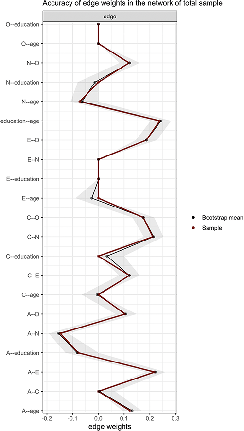
As illustrated in Figure 2, the horizontal axis represents the estimated edge weights, while the vertical axis enumerates each edge within the total sample network. The dark red line depicts the estimated edge weights in the total sample network, the black line indicates the bootstrap mean, and the gray area represents their bootstrapped confidence intervals. The accuracy tests reveal that the confidence intervals are relatively narrow, with bootstrap mean values closely aligning with the edge weights estimated by the psychological network analysis, and all estimated edge weights fall within their respective confidence intervals. This suggests a high degree of accuracy in the network estimation.
Estimated edge weights, bootstrap mean, and confidence intervals in the total sample network. The dark red line in the figure represents the estimated edge weights in the total sample network, the black line indicates the bootstrap mean, and the gray area shows their bootstrapped confidence intervals. Each horizontal line represents one edge of the network.
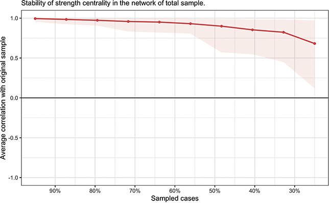
For the stability tests, as shown in Figure 3, the horizontal axis represents the decrease in sample size (as a percentage of the total sample). Each data point on the vertical axis signifies the average correlation between the edge strengths in the original network (estimated from 100 percent of the original sample) and those estimated from the reduced sample. A smaller trend of decreasing correlation strength with reduced sample size indicates that the network estimation is less affected by sample size fluctuations, leading to more stable results. The network exhibits minimal stability decline. A notable decrease in the average correlation between edges in the subsample and original networks occurs only when the sample size drops below 30 percent of the original sample. Together, these accuracy and stability results indicate that the network estimation is reliable and trustworthy for interpretation.
Average correlations between centrality indices (strength) of networks sampled with persons dropped and the original sample. Lines indicate the means and areas indicate the range from the 2.5th quantile to the 97.5th quantile.

3.3.2 Network Visualization
The network visualization result is shown in Figure 4, where nodes represent different variables. Blue lines indicate positive associations between variables, while red lines indicate negative associations.
Network of personality traits in the total sample. (Note: The darker and thicker the edges, the stronger the correlation. Blue edges for positive and red ones for negative connections. Education for the subjects’ education level, A for Agreeableness, C for Conscientiousness, E for Extraversion, N for Neuroticism, and O for Openness.)
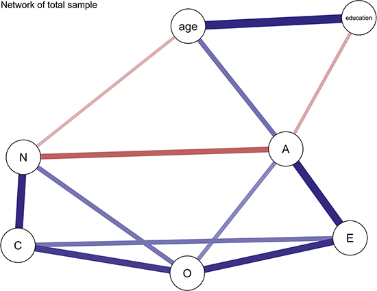
In the network, we observe that both education level and age show multiple associations with the Big Five personality traits. First, the relations among the five traits themselves include both positive and negative connections. For instance, we see a negative association between agreeableness and neuroticism, indicating that individuals with high agreeableness tend to be more emotionally stable and less affected by negative emotions. Fostering agreeableness in students may, therefore, contribute to greater emotional stability, enhancing their resilience to stress and interpersonal challenges. Students who develop qualities like cooperation and empathy may respond more calmly and constructively when facing academic pressure or peer conflicts.
We also observe that extraversion and neuroticism show no direct association, suggesting these two traits function independently in emotional and social behaviors. Extraversion reflects social activity levels, while neuroticism relates to the frequency and intensity of negative emotions. Therefore, an individual’s sociability does not necessarily influence their emotional stability. This implies that extraversion alone may not buffer or exacerbate emotional fluctuations, indicating that emotional stability might develop independently of social inclinations.
Furthermore, both age and education level show multiple connections with the Big Five traits. For instance, age is positively associated with agreeableness and negatively with neuroticism, but shows no link to openness. These variables also appear to co-occur with both agreeableness and neuroticism, suggesting they may be involved in broader patterns of psychological organization. For example, individuals with higher age or education tend to report higher agreeableness and lower neuroticism, which may reflect general developmental trends in emotional regulation and social maturity. However, since this study is based on cross-sectional data, no conclusions can be drawn about causal pathways or temporal progression.
These observed associations suggest that traits such as agreeableness and emotional stability may vary across age and education levels, reflecting differences that align with developmental stages. Rather than viewing these traits as fixed or uniformly distributed across ages, educators may consider tailoring emotional regulation and social skills programs to match students’ evolving capacities. For example, foundational interpersonal skills can be introduced in primary education, with progressively more nuanced training – such as conflict resolution, empathy development, or stress management – integrated into secondary education. This staged approach aligns with the variation observed in network patterns and supports the age-appropriate development of psychological resilience and prosocial behavior.
3.3.3 Centrality Indices
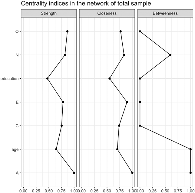
We analyzed the centrality indices for network of the total sample, including strength, closeness, and betweenness centrality, as shown in Figure 5.
Relative centrality indices of nodes in network of total sample.

Figure 5 Long description
From left to right, the three subfigures represent strength centrality, closeness centrality, and betweenness centrality, respectively. In terms of strength centrality, the nodes’ centrality from highest to lowest are: Agreeableness, Openness, Neuroticism, Extraversion, Conscientiousness, age, and education. For closeness centrality, the nodes’ centrality from highest to lowest are: Agreeableness, Extraversion, Neuroticism, Openness, Conscientiousness, age, and education. In betweenness centrality, the nodes’ centrality from highest to lowest are: Agreeableness, age, Neuroticism, Openness, Conscientiousness, Extraversion, and education.
In the total sample, the centrality analysis reveals the distinct roles of variables within the network. Agreeableness emerges as the most central variable, exhibiting the highest strength, closeness, and betweenness centrality, which highlights its pivotal role in directly and indirectly connecting with other variables. Openness ranks second in strength centrality, indicating its strong direct associations.
Both neuroticism and extraversion demonstrate high closeness centrality, suggesting they maintain strong indirect connections with other variables, positioning them as key players with broad connectivity in the network’s overall structure. In contrast, Conscientiousness occupies a middle position in strength and closeness centrality but has low betweenness, reflecting moderate direct influence but limited bridging capability.
Interestingly, age shows low strength and closeness centrality but stands out with the highest betweenness centrality, suggesting it plays a pivotal bridging role, facilitating connections between otherwise unlinked variables. Finally, education consistently shows low scores across all centrality measures, indicating it remains on the periphery of the network with limited influence or connectivity.
3.3.4 Network Comparison
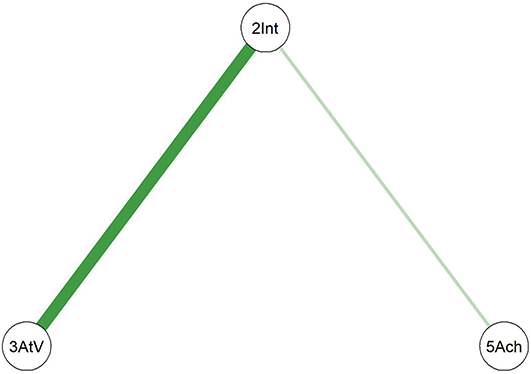
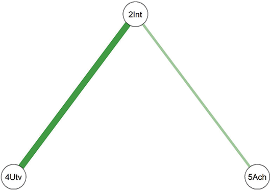
In this example study, we selected adult participants and divided them into two subsamples: early adulthood (18–30 years) and mid-adulthood (31–60 years). Separate networks were fitted for each subsample, and the differences in the network structures between the two groups were analyzed. The fitted network results for both subsamples are shown in Figure 6.
Networks of the young adults and the middle-aged adults. (Note: The darker and thicker the edges, the stronger the correlation. Blue edges for positive and red ones for negative connections. Education for the subjects’ education level, A for Agreeableness, C for Conscientiousness, E for Extraversion, N for Neuroticism, and O for Openness.)
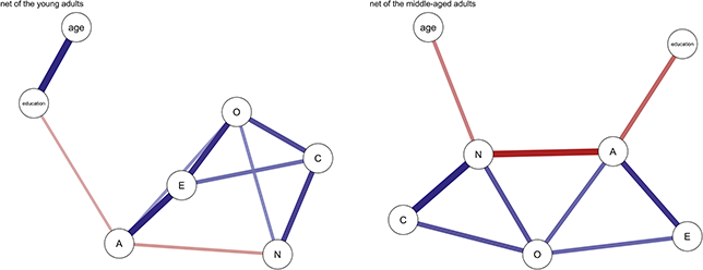
Figure 6 Long description
Comparing the two diagrams, some similar edges are observed, including Education-Agreeableness (negative), Agreeableness-Extraversion (positive), Extraversion-Openness (positive), Openness-Conscientiousness (positive), Conscientiousness-Neuroticism (positive), Neuroticism-Agreeableness (negative), and Neuroticism-Openness (positive). However, the connection between Conscientiousness and Extraversion is present only in the young adult network.
To compare the psychological networks of the young adult group (18–30 years) and the middle-aged group (31–60 years), we conducted a network comparison analysis focusing on network structure invariance, global expected influence, and differences in individual edges (see supplementary Figure 1 for detailed results).
The network structure invariance test revealed no statistically significant difference between the overall structures of the two age groups (M = 0.147, p = 0.194), indicating that the presence or absence of edges was largely comparable across groups. However, the comparison of global strength – a summary metric that reflects how strongly nodes are interconnected throughout the network – showed a significant difference. In this analysis, global strength was operationalized using global expected influence, which captures the sum of edge weights for all nodes while maintaining the sign (positive or negative) of each connection. This metric is particularly appropriate when networks include both positive and negative associations, as it offers a more nuanced view of overall network integration than traditional centrality indices (Robinaugh et al., Reference Ren, Wang and Wu2016).
Results indicated that the young adult group exhibited higher global expected influence (EI = 1.03) compared to the middle-aged group (EI = 0.63; S = 0.401, p = 0.017), suggesting that psychological constructs such as personality traits and demographic factors are more strongly interrelated in the younger group. In contrast, the middle-aged group displayed comparatively weaker overall connectivity. Additionally, edge-level comparisons revealed several significant differences in specific associations across the two age groups (see Supplementary Figure 1 for details).
In summary, although the overall network structures of the two age groups are similar, differences in global influence and specific edges – particularly the relation between agreeableness and neuroticism – highlight important age-related changes. These findings underscore the value of network comparison techniques in capturing nuanced developmental changes within psychological systems.
4 Psychological Network Analysis with Cohort Data: A Case Illustration
4.1 Introduction
This section aims to showcase the analytical process of cohort data and the application of network comparison techniques in uncovering variable relations. This section serves as a demonstration, offering an overview of the process rather than a comprehensive tutorial. For more detailed explanations and methodologies, readers are encouraged to read this open-access article (Tang, Lee, et al., Reference Tang, Lee, Wan, Gaspard and Salmela-Aro2022).
The study aimed to advance the understanding of motivational constructs by leveraging Situated Expectancy-Value Theory (SEVT; Eccles & Wigfield, Reference Eccles and Wigfield2020) to focus on the interactive relations among motivational variables and explore how these relations vary across different contexts, including grade levels, subject domains, and countries. Through this illustration, we aim to highlight the potential of psychological network analysis in contextualized motivation research and provide new insights and tools for developmental and educational sciences.
In this Element, we focus specifically on grade levels as the primary context for analyzing cohort data. Grade levels serve as a natural cohort framework that we leverage to explore the impact of specific contextual factors. Students within the same grade share developmental stages, educational environments, and similar experiences, making grade level a crucial factor for creating and analyzing our cohort data. Thus, by comparing network structures across different grade-level cohorts, we can reveal how context influences variable relations in educational and psychological phenomena.
4.2 Research Context
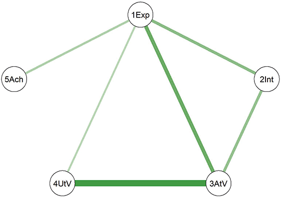
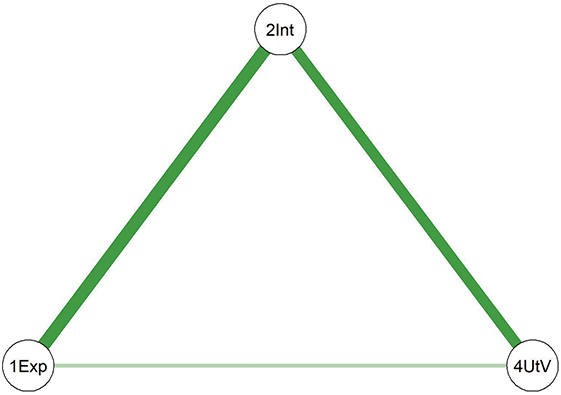
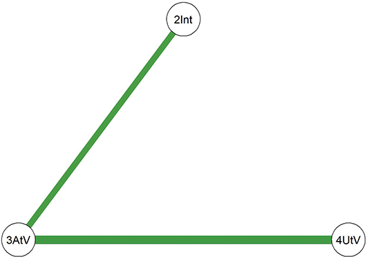
Eccles and Wigfield (Reference Eccles and Wigfield2020) emphasized the situated and dynamic nature of motivation, underscoring the importance of contextual and cultural influences on motivation. They highlighted the need to explore how expectancies and values interact across different situations, as this understanding is critical for designing effective motivational interventions. SEVT identifies two key motivational constructs: expectancies for success (e.g., “Can I do it?”) and subjective task values (e.g., “Do I want to do it?”). Expectancies for success represent individuals’ beliefs about their ability to succeed in a given task, often intertwined with self-concept. Subjective task values, on the other hand, encompass four dimensions: intrinsic value (i.e., enjoyment derived from the task), attainment value (i.e., relevance to identity), utility value (i.e., usefulness for short- or long-term goals), and cost (i.e., perceived sacrifices or trade-offs associated with the task). These constructs are robust predictors of students’ academic performance and choices.
4.3 Research Method
4.3.1 Samples and Variables
This study examined expectancies for success, subjective task values (i.e., intrinsic value, attainment value, utility value, and cost), and academic achievement within the framework of SEVT. Data were drawn from two cohorts:
Finnish Sample: Longitudinal data across Grades 6–9, involving 747–853 students per grade.
German Sample: Cross-sectional data from Grades 6–9, involving 103–123 students per grade.
The datasets used in this study reflect distinct cohort characteristics that complement each other in exploring developmental and contextual influences. The Finnish dataset represents a longitudinal cohort, tracking the same group of students from Grades 6 to 9 and capturing developmental changes in motivational beliefs and achievements over time. In contrast, the German dataset adopts a cross-sectional cohort design, sampling different groups of students across Grades 6–9, offering a snapshot of motivational patterns at each grade level. These cohort characteristics enable both a dynamic understanding of individual trajectories and situational comparisons across educational stages and cultural contexts.
For a detailed description of the variables, sampling procedures, and additional methodological considerations, readers are encouraged to read the open-access article (Tang, Lee, et al., Reference Tang, Lee, Wan, Gaspard and Salmela-Aro2022).
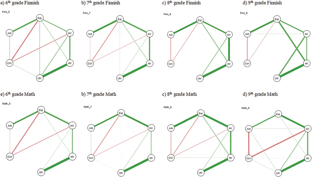
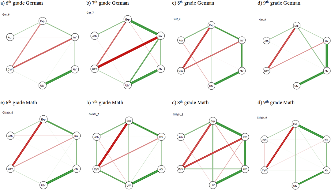
4.3.2 Network Analysis
In this study, the networks of expectancies, subjective task values, and achievement were analyzed for each grade, domain, and country using the qgraph package in R (Epskamp et al., Reference Epskamp, Cramer and Waldorp2012). These networks represent the relations among variables as partial correlations (edges) between pairs of variables (nodes), taking into account all other variables. To ensure interpretability, the networks were regularized using the graphical LASSO algorithm (Least Absolute Shrinkage and Selection Operator). This method applies the extended Bayesian information criterion (EBIC; Epskamp, Waldorp, et al., Reference Epskamp, Waldorp, Mõttus and Borsboom2018; Epskamp & Fried, Reference Epskamp and Fried2018) with a default gamma parameter of 0.5, resulting in sparse models where the absence of an edge signifies conditional independence between variables.
Additionally, exploratory graph analysis (EGA) was conducted using the EGAnet package (Golino & Epskamp, Reference Golino and Epskamp2017). EGA identifies clusters of closely connected nodes (variables) within the network, providing insights into how motivational constructs group together. For this purpose, the Louvain community detection algorithm was employed, as it has demonstrated superior performance compared to other algorithms, such as Walktrap (Christensen et al., Reference Christensen, Golino and Silvia2020).
4.3.3 Network Comparison
To compare the similarities and differences between networks, we conducted network comparison tests (NCT) using the NetworkComparisonTest package in R (van Borkulo et al., Reference Thissen, Steinberg and Kuang2023). This analysis allowed us to rigorously assess whether the structure and connectivity of networks varied across grades, domains, and countries. Specifically, two main invariance tests were employed to evaluate network differences.
The first test, the Network Structure Invariance Test (Test M), assessed whether the overall connection strength matrix differed between networks. This matrix captures the pattern and magnitude of connections between variables, providing a comprehensive view of structural variations. The second test, the Global Connectivity Invariance Test (Test S), examined the total strength of connections within each network, represented as the weighted sum of absolute connections. This test highlighted differences in the overall density or connectivity of the networks.
In addition to these high-level comparisons, we also performed individual edge comparisons to investigate specific differences in connections between nodes. This analysis focused on whether particular relations, such as the association between expectancies and intrinsic value, differed significantly across networks from different grades, domains, or countries. By identifying variations at the level of individual edges, this step offered a more detailed understanding of how variables interact differently in distinct contexts.
To ensure the reliability of these individual edge comparisons, p-values were adjusted using the Benjamini-Hochberg method (Thissen et al., Reference Tao, Hou and Niu2002). This adjustment accounted for the multiple comparisons performed, controlling for the false discovery rate and enhancing the robustness of the results.
The combination of these approaches provided a comprehensive understanding of network differences, from broad structural variations to specific edge-level distinctions. By uncovering these nuances, the analysis contributes to a more refined understanding of contextualized motivation research and informs the development of tailored educational interventions.
4.4 Findings
This section focuses on findings related to grade-level differences in motivational networks, examining how the relations between expectancy for success, subjective task values, and achievement evolve across grades. Although the study included cross-contextual comparisons across subjects and countries, this section highlights grade-level findings to illustrate the unique potential of cohort data for understanding differences in variable relations caused by various contextual factors (e.g., grade level).
Finnish Data: Finnish Language and Math Subjects across Grades
The global strength of Finnish language networks gradually declined from Grades 6 to 9. Specifically, significant structural differences emerged between the Grade 6 network and the Grade 8 and 9 networks. Key edge differences included the diminishing connection between intrinsic value and cost starting in Grade 8 and the weakening link between expectancy and utility value in Grade 9. These trends suggest that as students’ progress through grades, the motivational significance of intrinsic value and utility value for Finnish language learning wanes, reflecting possible shifts in focus toward external pressures or other priorities.
Networks of motivational constructs and their associations across grades for Finnish language and math subjects in Finland. Each subfigure represents the network for a specific subject at a given grade level. (Note: Green edges represent positive connections, red edges represent the negative connection. The thickness of the edges represents the strength of the connection. Exp = expectancies for success, InV = intrinsic value, AtV = attainment value, UtV = utility value, CsV = cost, and Ach = achievement.)

Figure 7 Long description
In the sixth-grade Finnish language network (a), Exp has connections with Ach, InV, UtV, and CsV. InV is connected to AtV and UtV. AtV is connected to UtV. UtV has connections with CsV and Ach. CsV is also connected to Ach. The seventh-grade shows similar connection patterns, with all these links remaining visible. In the eighth grade, most patterns are consistent, but the InV-CsV connection appears absent. The ninth-grade shows further evolution, where the UtV-CsV connection also appears to have disappeared. Moving to the Math networks: in the sixth-grade, Exp is connected to Ach, InV, UtV, and CsV. InV has connections with AtV and UtV. AtV is connected to UtV. UtV has connections with CsV and Ach. CsV is also connected to Ach. The seventh-grade largely mirrors Grade 6. In the eighth-grade, core patterns persist, including Exp-Ach, Exp-InV, Exp-UtV, Exp-CsV, and InV-AtV, InV-UtV. By the ninth-grade, these core patterns remain present, indicating overall stability in connectivity.
Networks of motivational constructs and their associations across grades for German language and math subjects in Germany. Each subfigure represents the network for a specific subject at a given grade level.
Note: Green edges represent positive connections; red edges represent the negative connection. The thickness of the edges represents the strength of the connection. Exp = expectancies for success, InV = intrinsic value, AtV = attainment value, UtV = utility value, CsV = cost, and Ach = achievement.) [Tang, X., Lee, H. R., Wan, S., Gaspard, H., & Salmela-Aro, K. Situating Expectancies and Subjective Task Values Across Grade Levels, Domains, and Countries: A Network Approach. AERA Open. (8) Copyright © [2022] (Xin Tang). Reprinted by permission of SAGE Publications]

Figure 8 Long description
The top row (a to d) shows German language networks from Grades 6 to 9. In the sixth-grade German network (a), Exp is connected to Ach, InV, UtV, and CsV; InV to AtV and UtV; AtV to UtV; UtV to CsV and Ach; and CsV to Ach. The seventh-grade German network (b) shows similar patterns. The eighth-grade German network (c)’s connection patterns are similar to Grade 7. The ninth-grade German network (d)’s patterns are similar to Grade 8. The bottom row (e to h) shows Math networks from Grades 6 to 9. In the sixth-grade Math network (e), Exp is connected to Ach, InV, UtV, and CsV; InV to AtV and UtV; AtV to UtV; UtV to CsV and Ach; and CsV to Ach. The seventh-grade Math network (f) shows similar patterns. The eighth-grade Math network (g)’s connection patterns are similar to Grade 7. The ninth-grade Math network (h)’s patterns are similar to Grade 8.
In contrast to the Finnish language, the global strength of math networks increased from Grade 6 to Grade 7 and remained stable afterward. Statistically significant structural differences appeared across grade pairs, particularly between Grades 6 and 9. Notably, utility value gained importance in Grade 9, emerging as a stronger influence, whereas the role of expectancies weakened. These changes highlight how students’ math motivations shift, with utility value becoming more central as students approach critical academic transitions like graduation.
German Data: German Language and Math Subjects across Grades
Although the global strength of German language networks followed an inverted U-shaped trend (peaking in Grade 7), no statistically significant differences in global strength were observed across grades. Structural differences were identified between Grades 6 and 9 and Grades 7 and 9. In Grade 9, intrinsic value exhibited stronger connections with attainment value but weaker ties to expectancy and cost. These findings suggest that older students increasingly prioritize the personal importance of the subject over their ability perceptions or the effort required.
Similar to German language, math networks displayed an inverted U-shaped trend in global strength, peaking in Grades 7 and 8. Statistically significant structural differences emerged between Grades 6 and 7, Grades 7 and 8, and Grades 7 and 9. Utility value began to connect with expectancy in Grade 7 and showed positive connections with cost during the same grade, reflecting a greater integration of external utility perceptions into students’ motivational systems at this stage. However, in Grade 8, intrinsic value exhibited a stronger connection with attainment value but a weaker and even negative association with utility value, suggesting nuanced shifts in students’ motivational priorities as they mature.
4.5 Implications for Cohort Data Analysis
The findings demonstrate that cohort data provides invaluable insights into the dynamic evolution of motivational systems across grades. Grade levels serve as a natural cohort framework that we leverage to explore the impact of specific contextual factors. Students within the same grade share developmental stages, educational environments, and similar experiences, making grade level a crucial factor for creating and analyzing our cohort data. Thus, by comparing network structures across different grade-level cohorts, we can reveal how context influences variable relations in educational and psychological phenomena.
The ability to detect changes in global network strength, structural patterns, and individual edge differences highlights the developmental trajectory of motivational variables. For example, the declining role of intrinsic value in older grades suggests the need for interventions that sustain students’ interest and enjoyment, especially in later stages of education. Similarly, the rising prominence of utility value in math underscores its role in shaping students’ future-oriented academic decisions. These findings provide critical insights for designing targeted educational interventions that align with students’ evolving motivational needs.
5 Psychological Network Analysis with Longitudinal Data
5.1 Overview
Developmental researchers often investigate lifespan changes by collecting longitudinal data, which involves repeated measurements from the same individuals over multiple time points. Broadly speaking, two temporal research designs are commonly employed: longitudinal panel designs and intensive longitudinal designs (Collins, Reference Collins2006). These correspond to two types of longitudinal data discussed in the literature: panel data, which consist of repeated assessments across relatively wider intervals (e.g., months or years) for multiple individuals, and time series data, which capture high-frequency observations (e.g., daily or hourly) from a single or few individuals. Though both types enable examination of within-person change, the latter provides greater temporal granularity and is particularly suited for modeling fine-grained dynamic processes.
Applying psychological network analysis to longitudinal data enables researchers to model how variables evolve over time, uncovering dynamic interdependencies and revealing patterns of co-regulation, accumulation, or destabilization among psychological constructs. This approach provides a powerful means for studying the complex, multivariate nature of human development (Card & Little, Reference Card and Little2007; Ferrer & McArdle, Reference Ferrer and McArdle2010), especially in contexts where traditional models fall short of capturing time-sensitive interactions.
In longitudinal psychological network analysis, repeated measurements allow for the construction of three complementary types of networks, each providing distinct insights into developmental dynamics. Among these, the temporal network plays a central role. It models time-lagged relations between variables across successive time points, offering a detailed picture of how psychological states or traits evolve and influence one another over time (Borsboom, Deserno, et al., Reference Borsboom, Deserno and Rhemtulla2021; Epskamp, Waldorp, et al., Reference Epskamp, Waldorp, Mõttus and Borsboom2018). Specifically, autoregressive edges capture the stability or inertia of a variable over time, and cross-lagged edges represent the predictive influence of one variable on another at a future time point. These lagged associations are particularly valuable for identifying dynamic regulatory mechanisms and for generating hypotheses about potential causal directions in developmental processes.
Moreover, by nesting repeated observations within individuals, temporal network models can distinguish within-person dynamics from between-person variability – a critical distinction for understanding individual-level change and identifying personalized points of intervention (Borsboom, Deserno, et al., Reference Borsboom, Deserno and Rhemtulla2021). Such models are particularly valuable in uncovering the mechanisms underlying symptom progression, behavioral escalation, or motivational feedback loops (Jordan et al., Reference Jones, Mair and McNally2020).
Complementing the temporal network, the contemporaneous network captures within–time point associations after accounting for lagged effects. These undirected networks reveal momentary co-activation patterns, such as how anxiety and motivation may fluctuate together during a stressful task, without assuming causal direction.
Lastly, the between-subjects network aggregates data across time points and participants, reflecting average associations among variables at the population level. This undirected network highlights trait-like patterns and serves as a useful bridge to compare findings with prior cross-sectional studies (Epskamp, Waldorp, et al., Reference Epskamp, Waldorp, Mõttus and Borsboom2018).
Together, these three network types provide a layered framework for modeling developmental processes – offering insights into both individual-level change and group-level structure across time.
This section outlines the application of longitudinal psychological network analysis in developmental and educational contexts. It first introduces key techniques for modeling longitudinal psychological networks. Building on this foundation, we present two illustrative case studies that demonstrate how to apply these techniques to different types of longitudinal data: panel data and time series data. Each example includes detailed steps for data preparation, network estimation, and result interpretation.
5.2 Techniques for Longitudinal Network Construction
The modeling of longitudinal psychological networks primarily relies on graphical vector autoregression (GVAR) models, which estimate lagged effects to capture dynamic associations across time points (Epskamp, van Borkulo, et al., Reference Epskamp and Fried2018; Epskamp, Waldorp, et al., Reference Epskamp, Waldorp, Mõttus and Borsboom2018). The VAR models can be used to estimate multivariate repeated measures by extending the autoregressive model to include lagged regressions of multivariate data. This approach incorporates measurements at both the current time point (t) and the previous time point (t-1).
In general, GVAR models are suited for panel data with fewer measurement points. However, GVAR encounters significant challenges in addressing multivariate multilevel data, such as distinguishing between within-individual and between-individual effects, due to its two principal assumptions (Epskamp, Waldorp, et al., Reference Epskamp, Waldorp, Mõttus and Borsboom2018). First, the time interval between successive measurements is approximately equal, known as temporal equidistance (Epskamp, Waldorp, et al., Reference Epskamp, Waldorp, Mõttus and Borsboom2018). Temporal equidistance is pivotal for interpreting temporal networks, as it delineates the time frame in which variable dynamics evolve. Second, the GVAR model presumes that the mean and variance of the time series data remain constant, implying stationarity. A stationary time series indicates that the data’s mean, variance, and auto-correlation are stable over time (Epskamp, Waldorp, et al., Reference Epskamp, Waldorp, Mõttus and Borsboom2018; Jordan et al., Reference Jones, Mair and McNally2020). The Kwiatkowski–Phillips–Schmidt–Shin (KPSS) unit root test can evaluate this stationarity (Contreras et al., Reference Contreras, Valiente, Heeren and Bentall2020; Kwiatkowski et al., Reference Jordan, Winer and Salem1992). If the data are not stationary, adjustments such as detrending can mitigate linear time trends by analyzing the residuals in the VAR model (Fried et al., Reference Fried, Papanikolaou and Epskamp2022).
To address these limitations, Epskamp et al. (Reference Epskamp, Deserno and Bringmann2024) introduced improvements to the GVAR framework by developing mlVAR model. This approach incorporates multilevel modeling techniques to distinguish within-individual effects from between-individual effects. Nevertheless, mlVAR requires more intensive data collection, with multiple observations per individual (typically at least 20), to ensure model robustness and accuracy (Epskamp et al., Reference Epskamp, Deserno and Bringmann2024).
Additionally, the organization of data in long format is critical for longitudinal psychological network analysis. In the long format, each row in the dataset represents a unique observation from a specific individual at a specific time point. Variables for these observations are distributed across columns, such as the measured psychological constructs, time identifiers, and participant identifiers. This format allows researchers to model temporal relations (e.g., how variables at time t−1 predict outcomes at time t) and contemporaneous networks (e.g., relations between variables within the same time frame).
Furthermore, another important aspect of psychological network modeling is parameter tuning, which involves adjusting specific parameters to control model complexity and improve interpretability. A commonly used approach is graphical LASSO, which estimates network model by applying a penalty that shrinks small or unstable edge weights toward zero. This penalty is controlled by the tuning parameter λ (lambda), which determines how aggressively weaker edges are reduced: Higher values of λ result in sparser networks by removing weaker connections, whereas lower values retain more edges, potentially at the cost of overfitting (Friedman et al., Reference Friedman, Hastie and Tibshirani2008; Hastie et al., Reference Hastie, Tibshirani, Friedman, Hastie, Tibshirani and Friedman2009).
To select the optimal model, the Extended Bayesian Information Criterion (EBIC) is often used in combination with graphical LASSO. EBIC introduces a second tuning parameter, γ (gamma), which adjusts the balance between model fit and sparsity. Ranging from 0 to 0.5, a higher γ places greater emphasis on parsimony, yielding simpler networks, whereas a lower γ favors richer models with more edges (Foygel & Drton, Reference Foygel and Drton2010). For example, in their study on adolescent suicide risk, Y. Li and Kwok (Reference Li, Deng and Xu2023) applied the EBICglasso method to reduce false positives and identify the most meaningful nodes and edges in a high-dimensional dataset. By carefully tuning λ and γ, they were able to produce a more stable and interpretable network structure, well-suited for identifying central psychological symptoms and risk factors.
5.3 Example Analysis Using R
To construct a temporal network, the most direct method is to center each variable within individuals and combine the centered data across all individuals to estimate a single graphical VAR model (A.-M. Isvoranu et al., Reference Isvoranu and Epskamp2022). This process has been simplified in the mlGraphicalVAR function of the graphicalVAR package by setting the idvar parameter to isolate the responses of one individual from those of another (Epskamp, van Borkulo, et al., Reference Epskamp, van Borkulo and van der Veen2018; Epskamp, Waldorp, et al., Reference Epskamp, Waldorp, Mõttus and Borsboom2018). Although these methods provide robust estimates of the fixed effects structure, they may not fully address the hierarchical nature of the data. Epskamp et al. (Reference Epskamp, Deserno and Bringmann2024) extended the univariate estimation by using univariate multilevel modeling approaches, distinguishing between within-individual and between-individual effects. These approaches were incorporated into the mlVAR package. This method estimates associations among each variable to its lagged variables and individual means using univariate multilevel models. It allows for the estimation of temporal and between-subject networks while using residuals to estimate contemporaneous networks. However, its limitation is that to accurately estimate the within-person mean, there must be multiple observations for each individual, usually at least around twenty. Thus, this methodology is more suitable for datasets with intensive temporal measurements rather than panel data.
In this section, we will demonstrate the construction of longitudinal networks using panel data and time-intensive data using the graphicalVAR package and the mlVAR package, respectively. All the codes and supplementary materials can also be accessed at https://osf.io/5n6v8/.
5.3.1 Panel Data
The mlVAR function estimates multivariate vector autoregressive (VAR) models for intensive longitudinal data. It outputs three distinct network structures: temporal networks, which represent lagged (e.g., lag-1) predictive relations between variables over time; contemporaneous networks, which capture within-time-point partial correlations after accounting for lagged effects; and between-subject networks, which model correlations across individuals’ average scores to reflect stable trait-level associations.
To visualize the estimated networks, the qgraph package can be used to generate intuitive graphical representations for each network type. Additionally, the networktools package supports further analysis, such as computing centrality indices to identify the most influential nodes in each network.
The function mlGraphicalVAR fits fixed effects temporal and contemporaneous networks for multiple subjects and runs separate graphicalVAR models. The model first pools all data, adds subject-centered variables, and runs graphicalVAR to obtain fixed effects. Next, it runs EBICglasso on individual means to obtain the between-subjects network. Finally, it runs graphicalVAR on each subject’s data to obtain individual networks. Users can use the qgraph package to plot network graphs for the three types of networks.
Simulated Data Generation
We used the mlVARsim function from the mlVAR package to simulate an mlVAR model and data with random variance-covariance matrix random effects. Here, “nPerson” represents the number of participants, “nNode” indicates the number of variables, “nTime” denotes the number of observations per participant, and “lag” specifies the maximum lag to be used. We simulated a panel dataset consisting of 200 participants, with 5 measurements each and 10 variables.
library("graphicalVAR")library("mlVAR")library("qgraph")set.seed(2025)
Model <- mlVARsim(nPerson =200, nNode = 10, nTime = 5, lag=1)write.csv(Model$Data, file="panel_data.csv")
Data Preparation
To download the dataset, go to the supplementary materials.
The relevant data file is called “panel_data.csv,” which can be loaded into R by using the default read.csv function.
panel <- read.csv("panel_data.csv",header = TRUE)vars <- c("V1","V2","V3","V4","V5","V6","V7","V8","V9","V10")idvar <- "ID"
Network Estimation
The mlVAR package is capable of estimating temporal networks, contemporaneous networks, and between-participant networks. We usually use “lmer” as the estimation method. Depending on the nature of the data, the mlVAR package provides several options for estimating time effects and contemporaneous effects. In temporal network, “correlated” estimates correlated random effects, “orthogonal” estimates non-correlated random effects and “fixed” estimates a model in which only the intercept is random. Defaults to “correlated” when the number of variables is less than 6 and “orthogonal” otherwise. In contemporaneous network, these networks are always estimated post hoc by investigating the residuals of the temporal models. “correlated” and “orthogonal” run second multilevel models in which the networks are estimated using node-wise estimation. “fixed” and “unique” simply correlate the residuals, either by computing one network for all subjects (fixed) or a single network per subject. In panel data, “gamma” is the EBIC tuning parameter.
res_GVAR <- mlGraphicalVAR(panel, vars, idvar = idvar, gamma = 0.5, subjectNetworks = FALSE)
Then, we can use the qgraph package to plot network graphs for the three types of networks and use the networktools package to compute network centrality. It allows users to avoid estimating false-positive associations by employing the conservative “AND” rule, which means edges are only included in the network if both coefficients are significant at a level of p < .05.
Temporal network:TN<- qgraph(res_GVAR$fixedPDC, layout = "circle",theme = "colorblind", title = "Temporal", labels = vars, vsize = 5, asize = 4)write.csv(TN$Arguments$input,file="matrixTN.csv")Contemporaneous network:CN<- qgraph(res_GVAR$fixedPCC, layout = "circle",theme = "colorblind", title = "Contemporaneous", labels = vars, vsize = 5, asize = 4)write.csv(CN$Arguments$input,file="cormatrixCN.csv")Between-subjects network:BN<- qgraph(res_GVAR$betweenNet, layout = "circle", theme = "colorblind", title = "Between-subjects", labels = vars, vsize = 5, asize = 4)write.csv(BN$Arguments$input,file="cormatrixBN.csv")
Result
Figure 9 illustrates the temporal network, where edges represent the predictive strength of nodes at time (t-1) on those at time (t), with arrows indicating the direction of prediction. The arrow directions provide insights into potential causal relations among nodes. The red circle near nodes implies the autoregression over time, suggesting the relative stability of these variables within the time intervals. However, since the panel data is purely simulated, the results were not interpreted in details.
Fixed effects temporal network model of variables v1-v10 in a simulated panel dataset. Edges represent prediction between nodes from one measurement point to the next measurement point that remain after controlling for all other variables at the previous measurement point. Blue lines depict positive associations and red lines depict negative associations between variables.
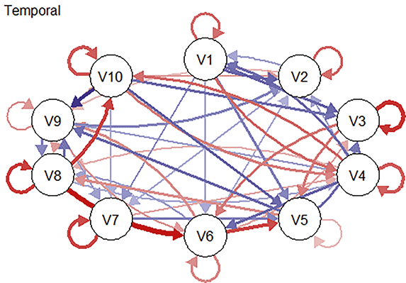
Figure 9 Long description
It consists of 10 circular nodes (V1 to V10) representing different variables. Arrows between nodes indicate the mutual influence of variables over time: blue arrows represent negative relationships, red arrows represent positive relationships, and the thickness of the arrows denotes the strength of the influence. Each node also features a self-loop arrow pointing back to itself, which shows the variable’s self-sustaining effect over time. The essence of this graph lies in visualizing the application of longitudinal data in network analysis, emphasizing the dynamic evolution of variables over time, rather than the psychological implications of specific variable relationships.
Figure 10 delineates the contemporaneous network, showing the interrelations between variables within the same time frame while controlling for other temporal and contemporaneous links.
Fixed effects contemporaneous network model of variables v1-v10 in a simulated panel dataset. Edges represent associations between the variables within the same time frame after controlling for temporal associations. Blue lines depict positive associations and red lines depict negative associations between variables.

Figure 11 outlines the between-subjects network, depicting the connectivity patterns among within-person means throughout the entire assessment period. These patterns can be compared with data from cross-sectional networks for further analysis.
Fixed effects between-subject network model of variables v1-v10 in a simulated panel dataset. Edges represent correlations between intra-individual mean levels, after controlling for the remaining variables in the network. Blue lines depict positive associations, and red lines depict negative associations between variables.

5.3.2 ESM Data
To illustrate the use of the mlVAR package in time-intensive network analysis, we will demonstrate the aforementioned functionalities by analyzing ESM data. In this case, the ESM data were simulated from individuals with test anxiety (N = 118) collected over seven days before an exam.
Participants and Procedure
Sample were college candidates for the College English Test Band 4 (CET-4) and Band 6 (CET-6) exams held on December 18, 2021, nationwide through social media platforms. We used the Test Anxiety Scale (TAS) to screen individuals with moderate or higher levels of test anxiety (TAS > 11; Sarason, Reference Samra, França, Lucassen and Waterhouse1978). A time-based sampling method for experience sampling (Swendsen et al., Reference Speyer, Hall and Ushakova2000) was employed. For the seven days leading up to the exam, we divided each day into three time periods: morning (9:00–12:00), midday (12:00–15:00), and afternoon (15:00–18:00). One random time point was sampled within each period, resulting in 21 momentary measurement points for each participant. Participants were required to complete the questionnaire within 40 minutes; otherwise, it was considered invalid. We excluded participants with more than 20 percent invalid responses (Shiffman et al., Reference Sarason, Spielberger and Sarason2008; Smith & Juarascio, Reference Shiffman, Stone and Hufford2019). In the end, 118 participants were included in the analysis. In the ecological momentary assessment, we used visual analog scales (VAS: 0 representing not at all, 100 representing very much) to measure participants’ exam confidence (How confident do you feel about the upcoming CET-4/CET-6 exam right now?), test anxiety (How anxious do you feel about the upcoming CET-4/CET-6 exam right now?), positive affect (How much positive emotion are you feeling right now?), and negative affect (How much negative emotion are you feeling right now?).
Data Preparation
To download the dataset, go to supplementary materials.
The relevant data file is called “esmdata.csv,” which can be loaded into R by using the default read.csv function.
library("mlVAR")library("qgraph")ESM <- read.csv("esmdata.csv",header = TRUE)
This loads the data in long format, which contains a column with subject id’s, four columns with the names of variables (confidence, test anxiety, positive affect, and negative affect, respectively). The “day” column refers to the number of days the experience sampling method was measured (range: 1 to 7), and the “beep” column refers to the number of times the ecological transient was measured during the day (range: 1 to 3). Next, we named the data:
names(ESM) <-c("X","confidence","test_anxiety","positive_affect","negative_affect","subject","day","beep")
Next, we need to name the data and convert all the aforementioned variables into vectors to be used in the analysis. “vars” refers to the vectors of variables to include in the analysis and “idvar” refers to string indicating the subject ID. “dayvar” refers to string indicating assessment day. Adding this parameter ensures that the first measurement of a day does not regress against the last measurement of the previous day. “beepvar” refers to optional string indicating assessment beep per day. Adding this parameter will cause non-consecutive beeps to be treated as missing.
vars <- c("confidence","test_anxiety","positive_affect","negative_affect")idvar <- "subject"dayvar <- "day"beepvar <- "beep"
Network Estimation
Similar codes in panel data were executed for ESM data.
res_mlVAR1 <- mlVAR(ESM, vars, idvar, dayvar, beepvar, lags = 1,temporal = "default", contemporaneous = "default")Temporal network:TN<-plot(res_mlVAR1, "temporal", layout = "circle", nonsig = "hide", theme = "colorblind", title ="Temporal", labels = vars, vsize = 15, rule = "and", asize = 5, mar = c(10,10,10,10))write.csv(TN$Arguments$input,file="matrixTN.csv")Contemporaneous network:CN<-plot(res_mlVAR1, "contemporaneous", layout = "circle", nonsig = "hide", theme = "colorblind", title ="Contemporaneous", labels = vars, vsize = 15, rule = "and", asize = 5, mar = c(10,10,10,10))write.csv(CN$Arguments$input,file="cormatrixCN.csv")Between-subjects network:BN<-plot(res_mlVAR1, "between", layout = "circle", nonsig = "hide", theme = "colorblind", title = "Between-subjects", labels = vars, vsize = 15, rule = "and", asize = 5, mar = c(10,10,10,10))write.csv(BN$Arguments$input,file="cormatrixBN.csv")
Result
Figure 12 illustrates the temporal network for the ESM data. All nodes exhibit positive autoregression over time, suggesting the relative stability of these variables within short intervals (approximately every 3 hours). The arrow directions provide insights into potential causal relations among nodes. For example, exam anxiety positively influences positive emotions, and there is a positive feedback loop between positive affect and confidence. This dynamic might be due to exam anxiety motivating study behaviors, which lead to positive experiences and enhanced confidence. However, since this dataset is simulated, further exploration of this phenomenon is not conducted.
Temporal network model of emotional and confidence variables in a simulated test anxiety ESM dataset. Edges represent prediction between nodes from one measurement point to the next measurement point that remain after controlling for all other variables at the previous measurement point. Blue lines depict positive associations and red lines depict negative associations between variables.

Figure 13 delineates the contemporaneous network, revealing notable associations such as robust connections between positive emotions and negative emotions, between negative emotions and exam anxiety, and between self-confidence and positive emotions. Particularly noteworthy is the negative correlation between positive emotions and exam anxiety in the contemporaneous network. This contrast with the temporal network’s pattern suggests potential shifts in individuals’ behaviors across different time lags.
Contemporaneous network model of emotional and confidence variables in a simulated test anxiety ESM dataset. Edges represent associations between the variables within the same time frame after controlling for temporal associations. Blue lines depict positive associations and red lines depict negative associations between variables.
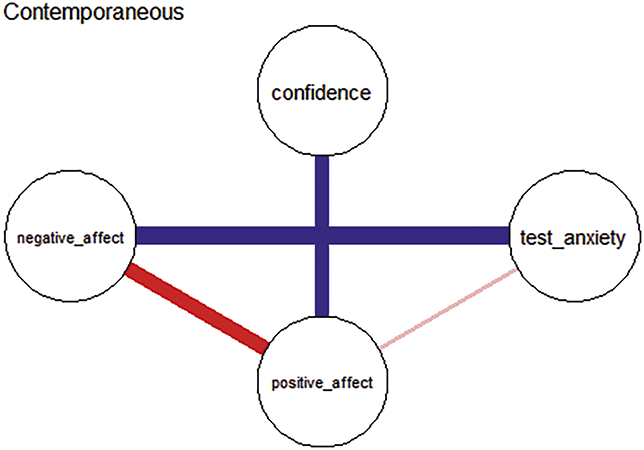
Figure 14 depicts the between-subjects network, showing patterns among within-person means throughout the entire ecological momentary assessment period.
Between-subject network model of emotional and confidence variables in a simulated test anxiety ESM dataset. Edges represent correlations between intra-individual mean levels, after considering the remaining variables in the network. Blue lines depict positive associations, and red lines depict negative associations between variables.

6 Causal Inference Using Directed Acyclic Graphs
6.1 Introduction
Understanding causality is a central goal in psychological and educational research, yet establishing cause-and-effect relations is often constrained by practical limitations. For instance, researchers may wish to explore whether a student’s intrinsic motivation influences their academic performance, or whether the reverse is true. In many real-world contexts – where randomized controlled trials are not feasible – directed acyclic graphs offer a valuable framework for articulating and examining such causal hypotheses using observational data. In a directed acyclic graph, nodes represent observed or latent variables, directed edges (arrows) indicate potential causal influences, and the acyclic property ensures that no feedback loops exist – meaning a variable cannot indirectly cause itself.
To construct a directed acyclic graph, researchers typically begin by estimating a zero-order correlation network, which captures raw associations among variables without controlling for others. This is then contrasted with a partial correlation network, in which each pairwise relation is adjusted for all remaining variables in the system. The key idea is that patterns of conditional dependence and independence offer clues about the likely direction of influence. Based on this logic, causal discovery algorithms – such as the Inferred Causation Algorithm (ICA; Pearl, Reference Panayiotou, Black, Carmichael-Murphy, Qualter and Humphrey1988; Pearl & Verma, Reference Pearl1995) – are applied to identify structural motifs such as colliders (e.g., A → C ← B) and confounders (e.g., A ← C → B). These structures help researchers infer which variables may act as causes, effects, or mediators within a system. Though the process relies on cross-sectional data, it provides a principled statistical foundation for generating testable causal hypotheses. Readers interested in the formal rules underlying directed acyclic graph inference are encouraged to consult Section 2.3.2, which elaborates on the assumptions and constraints of this approach.
Directed acyclic graphs offer distinct advantages that complement both traditional causal models, such as randomized controlled trials and cross-lagged panel models. One notable strength lies in their efficiency and accessibility: Directed acyclic graphs allow researchers to infer potential causal pathways from cross-sectional data, making them particularly appealing in settings where longitudinal data or experimental manipulation is unavailable. Moreover, unlike traditional structural equation modeling, which would require manually testing a vast number of possible models, directed acyclic graph-based algorithms such as the Inferred Causation Algorithm can systematically and computationally derive plausible structures based on patterns of conditional dependence.
Directed acyclic graphs also differ conceptually from both undirected and lag-based directed networks. Though undirected networks capture the structure of conditional associations, they remain agnostic about directionality and causality. Temporal networks rely on temporal ordering to infer influence, and include autoregressive effects that capture a variable’s stability over time. Directed acyclic graphs, however, infer directionality based on conditional independence patterns, rather than time. As a result, directed acyclic graphs do not include self-loops or autoregressive paths, and their directed edges reflect hypothesized causal flows grounded in statistical reasoning rather than empirical time lags. Though it should be noted that directed acyclic graphs cannot directly prove causality, they offer a directional framework for mapping potential causal pathways, serving as a cost-effective method for inferring causal hypotheses among variables (Lee et al., Reference Larson2024; Rohrer, Reference Robinaugh, Millner and McNally2018). This makes directed acyclic graphs especially well-suited for theorizing about the structure of psychological systems where causal directions are unknown or hypothesized.
To demonstrate the practical steps of directed acyclic graph construction and interpretation, this section draws on a representative study by Lee et al. (Reference Larson2024). The study explores the possible causal structures among key motivational constructs outlined in Situated Expectancy–Value Theory (SEVT), including expectancy for success, intrinsic value, attainment value, utility value, and prior achievement, based on cross-sectional survey data. We will guide readers through the directed acyclic graph modeling process and explain how the resulting graph can inform theory refinement and causal reasoning.
6.2 Step-by-Step Tutorial
To create directed acyclic graphs, scholars should follow these steps: (1) estimate undirected networks while using zero-order correlations; (2) estimate (default) undirected networks where the partial correlations were estimated; and (3) create directed networks or directed acyclic graphs using the ICA.
To demonstrate the steps, one study is used as an example (Lee et al., Reference Larson2024). Readers are encouraged to read the paper for further information. This study explored a set of plausible directed acyclic graphs representing the constructs involved in Situated Expectancy–Value Theory (SEVT) using cross-sectional data. Specifically, it is aimed to investigate the potential causal relations among expectancy for success, intrinsic value, attainment value, utility value, and prior achievement.
The demonstration data include five variables – Expectancies, Intrinsic Value, Attainment Value, Utility Value, and Achievement – from ninth-grade students. All the codes and supplementary materials can also be accessed at https://osf.io/5n6v8/.
6.2.1 Step 1: Estimating Zero-Order Correlation Network
Before constructing the directed acyclic graph, we begin by estimating an undirected network based on zero-order correlations. This provides a baseline view of the raw associations between variables, serving as a reference for identifying changes in connections once other variables are statistically controlled.
We start by calculating the zero-order correlations among Expectancies, Intrinsic Value, Attainment Value, Utility Value, and Achievement, and based on these, we construct a network of zero-order correlations. The significance of the edges is then tested using the SIN (Significant, Intermediate, Non-significant) algorithm, as it is crucial to establish the existence of associations before examining their directionality.
The SIN algorithm was implemented in R for the construction of the directed acyclic graph (Drton, Reference Drton2013). In reporting the results, we distinguish between statistically significant results (p < .05) and borderline significant results (.05 ≤ p < .10), consistent with common conventions in exploratory network research. This approach reflects the exploratory nature of directed acyclic graph estimation, which aims not to confirm pre-specified hypotheses, but to generate plausible causal models based on complex multivariate associations. Given that p-values are adjusted for multiple comparisons – making it more difficult to reach strict significance – reporting both significant and borderline significant findings allows for a more nuanced interpretation of edge relevance, especially when modeling high-dimensional psychological systems where suppressor effects, colliders, or mediators may influence statistical estimates (Amrhein et al., Reference Amrhein, Greenland and McShane2019; Drton & Perlman, Reference Drton and Perlman2008; Wasserstein et al., Reference Waldorp, Marsman and Maris2019).
The main code for this step is as follows:
# Load Required Librarieslibrary(qgraph) # For visualizing networkslibrary(ppcor) # For partial correlation analysislibrary(psych) # For psychometric computationslibrary(gtools) # For combination computationslibrary(SIN) # For SIN algorithmlibrary(corpcor) # For correlation and covariance matrix operations# Data loadingdag_demo_FS <- read.csv(file="your path/dag_demo_FS.csv")# Correlation and Partial Correlation Analysis# Compute Correlation Matrixdat.cor <- cor(dag_demo_FS, use = ‘pairwise.complete.obs‘)# Display Correlation Matrixprint(dat.cor)# Convert Correlation Matrix to Data Frame for Further Operationsdc <- as.data.frame(dat.cor)# Plot Correlation Networkqgraph( dc, layout = "spring", minimum = 0.2, title = "Correlation Network", diag = FALSE)# Define a SIN Algorithm-Based Test Functionsin.ag <- function(data, plot = TRUE, holm = TRUE, alpha = 0.1, beta = 0.5) { cov <- cov(data) # Compute Covariance Matrix n <- dim(data)[1] # Sample Size p <- dim(data)[2] # Number of Variables sin.amat <- sinUG(cov, n, holm = holm) # SIN Algorithm Application sin <- sin.amat sin.lt <- sin[lower.tri(sin, diag = FALSE)] # Extract Lower Triangle of Matrix if (plot) { # Generate Edges and Labels for Plot connect <- combinations(p, 2) lc <- dim(connect)[1] make.name <- function(a) paste(a[1], paste("-", a[2], sep = ""), sep = "") leg <- apply(connect, 1, make.name) # Plot P-Values for Edgesplot( sin.lt, pch = 16, bty = "n", axes = FALSE, xlab = "edge", ylab = "P-value")axis(1, at = 1:lc, labels = leg, las = 2)axis(2, at = c(0.2, 0.4, 0.6, 0.8, 1), labels = TRUE)lines(c(1, lc), c(alpha, alpha), col = "gray") # Add Threshold Line (alpha)lines(c(1, lc), c(beta, beta), col = "gray") # Add Threshold Line (beta)name <- deparse(substitute(data))title(main = paste(attr(data, "cond")), font.main = 1)text(1, 0.15, "0.1", col = "gray") # Annotate Alpha Thresholdtext(1, 0.55, "0.5", col = "gray") # Annotate Beta Threshold}# Adjust the Adjacency Matrix Based on Alpha Thresholdsin.amat[sin.amat < alpha] <- 2sin.amat[sin.amat != 2] <- 0sin.amat[sin.amat == 2] <- 1diag(sin.amat) <- 0names(sin.lt) <- leginvisible(list(pval = sin.lt, amat = sin.amat)) # Return Results}# Apply the SIN Algorithm Testdag_demo_FS <- as.data.frame(dag_demo_FS)dag_demo_FS <- drop_na(dag_demo_FS)test <- sin.ag(dag_demo_FS)
In the aforementioned code, we first computed the correlation coefficients among the five variables and visualized the correlation network as shown in Figure 15.
Zero-order correlation network of the five SEVT variables. “Exp” represents Expectancies, “Int” represents Intrinsic Value, “AtV” represents Attainment Value, “Utv” represents Utility Value, and “Ach” represents Achievement.
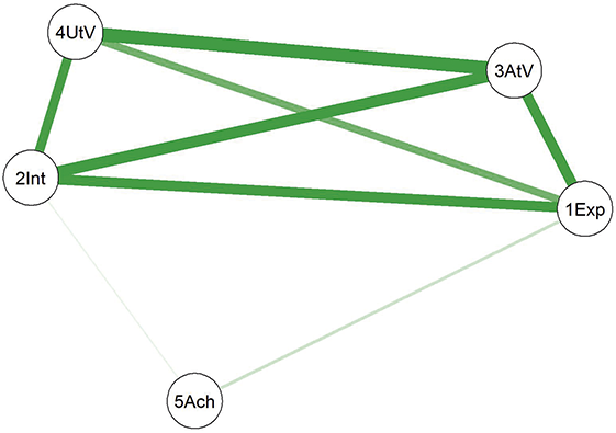
Subsequently, we implemented a function to test the significance of network edges based on the SIN algorithm. The results of the SIN algorithm’s edge significance testing for all network correlations are displayed in Figure 16.
Results of the edge significance test for the zero-order correlation network of the five SEVT variables. Points below the gray horizontal line indicate edges with a significance level below 0.1, suggesting they should be considered significant.
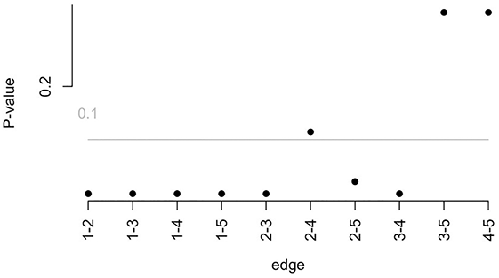
Thus, the following seven edges were identified as significant: expectancy for success and intrinsic value, expectancy for success and attainment value, expectancy for success and utility value, expectancy for success and prior achievement, intrinsic value and attainment value, intrinsic value and prior achievement, and attainment value and utility value.
6.2.2 Step 2: Estimating Partial-Correlation Network
Next, we estimate an undirected network using partial correlations. This step helps us identify which connections remain after accounting for the variance of all other variables, and allows us to detect potential confounding or mediating structures when compared to the zero-order correlation network.
Using mgm package (Haslbeck & Waldorp, Reference Haslbeck and Waldorp2015) in R, we estimate an undirected partial-correlation network using the Gaussian Graphical Model (Epskamp, Waldorp, et al., Reference Epskamp, Waldorp, Mõttus and Borsboom2018; Foygel & Drton, Reference Foygel and Drton2010). In this model, nodes represent the factor score variables from the first step, while edges represent partial correlation coefficients, controlling for all other variables. The code for fitting the network is as follows:
# Load the required librarylibrary(mgm)# Fit the network using mgmfit.all <- mgm( data = dag_demo_FS,  # Input dataset type = rep(‘g‘, 5),         # Specifies Gaussian variables for all 5 variables lambdaSeq = 0,                # No regularization lambdaSel = "EBIC"       # Use EBIC for model selection)# Visualize the network using qgraphqgraph( fit.all$pairwise$wadj,     # Weighted adjacency matrix from the mgm result threshold = 0.15,       # Threshold for edge inclusion labels = Labels        # Labels for the nodes
)
In the aforementioned code, we used the mgm function from the mgm package and visualized the results, as shown in Figure 16. The mgm() function from the mgm package is used to estimate network models, including Gaussian Graphical Models. In the given code, the function analyzes five continuous variables from the dataset dag_demo_FS, specifying all variables as Gaussian (type=rep(‘g’, 5)). By using the Extended Bayesian Information Criterion for regularization parameter selection (lambdaSel= “EBIC”) and applying no additional penalty (lambdaSeq=0), it identifies the relations between variables, represented as partial correlations in a weighted adjacency matrix. This function enables researchers to explore complex variable interactions, with results often visualized as a network graph to reveal underlying structures and direct connections.
When visualizing the network models, positive relations are indicated by green lines, whereas negative relations are indicated by red lines. The thickness of an edge indicates the strength of the association between two nodes, ranging from −1 to 1, where the absence of a line between two nodes represents no association.
According to the significance test results from the SIN algorithm (as shown in Figure 16), the statistically significant edges include: (1Exp–2Int, 1Exp–3AtV, 1Exp–4UtV, 1Exp–5Ach, 2Int–3AtV, 2Int–5Ach, and 3AtV–4UtV). In the partial correlation network (see Figure 17), six of these seven edges – excluding 2Int–5Ach – also appear. Therefore, these six edges are considered meaningful, having been supported by both the SIN algorithm and the partial correlation model. We thus selected these six overlapping edges as the basis for constructing the directed acyclic graph. This decision was motivated by two reasons: First, the dual confirmation enhances the robustness of the edge selection; second, it contributes to model simplicity by reducing the number of paths considered for interpretation.
The partial correlation network of the five SEVT variables fitted using the psychological network model. Exp represents Expectancies, Int represents Intrinsic Value, AtV represents Attainment Value, Utv represents Utility Value, and Ach represents Achievement.

6.2.3 Step 3: Creating Directed Acyclic Graphs
Building on the patterns of conditional independence observed in the previous step, we now apply the Inferred Causation Algorithm (ICA) to determine the directionality of associations. This step aims to construct a directed acyclic graph that represents plausible causal pathways between variables while preserving the acyclic structure.
To start drawing directionality for the directed acyclic graph, we should compare the zero-order correlation network (Figure 15) to the partial correlation network (Figure 17), and see which edges either “disappeared” or “appeared” between the two networks. Results found the following changes between the correlation and partial correlation network: (1) The connection between intrinsic value and utility value was gone in the partial correlation network (2Int-4UtV); and (2) the connection between intrinsic value and prior achievement was gone in the partial correlation network (2Int-5Ach).
The next step is to examine various combinations of variables to specifically assess their relations. To do this, we apply the ICA (Pearl, Reference Panayiotou, Black, Carmichael-Murphy, Qualter and Humphrey1988; Pearl & Verma, Reference Pearl1995) to infer the directionality of these significant edges. The ICA simplifies the process by first examining the conditional independence of two variables, and then determining if a third variable between them is a collider, by checking whether it is included in the set on which the two variables are conditioned. The steps are as follows:
a) For each pair of variables, a and b, investigate (a ⫫ b | Sab), which means looking for their conditional independence. Connect a and b with an edge if no Sab can be found, indicating dependency.
b) For a pair of variables with another variable between them (e.g., a-c-b), verify if c is part of Sab. If yes, continue; if no, then c is a collider, and the relation is a → c ← b.
c) Integrate as many undirected edges as possible without introducing new variable structures or cycles.
We now turn to the empirical example in this study to demonstrate how directional relations between nodes are determined. First, we inferred the directed connections within the directed acyclic graph using the Inductive Causation Algorithm, based on the disappearance of the association between intrinsic value and utility value in the partial correlation network (2Int-4UtV). Various possible combinations of variables were chosen during construction. For example, we examined the relations between (1) intrinsic value, utility value, and expectancy for success (2Int-4UtV-1Exp; refer to Figure 18), (2) intrinsic value, utility value, and attainment value (2Int-4UtV-3AtV; refer to Figure 19), and (3) intrinsic value, utility value, and prior achievement (2Int-4UtV-5Ach; refer to Figure 20).
Partial network that examines the relations among Intrinsic Value, Utility Value, and Expectancy for Success (2Int-4UtV-1Exp) using psychological network analysis.

Partial network that examines the relations among Intrinsic Value, Utility Value, and Attainment Value (2Int-4UtV-3AtV) using psychological network analysis.

Partial network that examines the relations among Intrinsic Value, Utility Value, and Prior Achievement (2Int-4UtV-5Ach) using psychological network analysis.
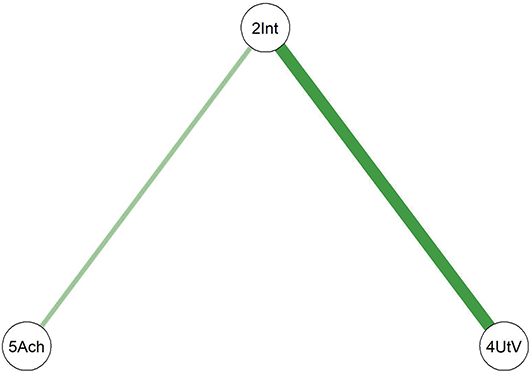
The code for fitting the partial networks of these nodes and their results is as follows:
# Fitting partial correlation networks for selected variable combinations# Fit for Intrinsic Value, Utility Value, and Expectancy for Success (2Int-4UtV-1Exp)fit.241 <- mgm( dag_demo_FS[, c(2, 4, 1)], type = rep(‘g‘, 3), lambdaSeq = 0, lambdaSel = "EBIC" # Gaussian variables with EBIC selection)Labels <- c("2Int", "4UtV", "1Exp")qgraph( fit.241$pairwise$wadj, threshold = 0.15, labels = Labels, title = "Intrinsic Value, Utility Value, and Expectancy for Success")
# Fit for Intrinsic Value, Utility Value, and Attainment Value (2Int-4UtV-3AtV)fit.243 <- mgm( dag_demo_FS[, c(2, 4, 3)], type = rep(‘g’, 3), lambdaSeq = 0, lambdaSel = "EBIC" # Gaussian variables with EBIC selection)Labels <- c("2Int", "4UtV", "3AtV")qgraph( fit.243$pairwise$wadj, threshold = 0.15, labels = Labels, title = "Intrinsic Value, Utility Value, and Attainment Value")
# Fit for Intrinsic Value, Utility Value, and Prior Achievement (2Int-4UtV-5Ach)fit.245 <- mgm( dag_demo_FS[, c(2, 4, 5)], type = rep(‘g‘, 3), lambdaSeq = 0, lambdaSel = "EBIC" # Gaussian variables with EBIC selection)Labels <- c("2Int", "4UtV", "5Ach")qgraph( fit.245$pairwise$wadj, threshold = 0.15, labels = Labels, title = "Intrinsic Value, Utility Value, and Prior Achievement")
By fitting partial correlation networks for different combinations of nodes, we were able to identify which variables contributed to the disappearance of the connection between intrinsic value and utility value. Specifically, we found that this connection vanished when attainment value was included in the network (refer to Figure 19).Therefore, we inferred that there could be a collider effect where both intrinsic value and utility value pointed to attainment value (2Int → 3AtV ← 4UtV). There was no need to examine the relations between four variables (e.g., 2Int4UtV-1Exp-3AtV or 2Int-4UtV-1Exp-5Ach or 2Int-4UtV3AtV-5Ach) because we already directed the lines.
Subsequently, we inferred the directed associations between nodes in the directed acyclic graph using the ICA, based on the disappearance of the association between intrinsic value and prior achievement in the partial correlation network. (2Int-5Ach). Again, we chose various possible combinations of variables. For example, we examined the relations between (1) intrinsic value, prior achievement, and expectancy for success (2Int-5Ach-1Exp; refer to Figure 21), (2) intrinsic value, prior achievement, and attainment value (2Int-5Ach-3AtV; refer to Figure 22), and (3) intrinsic value, prior achievement, and utility value (2Int-5Ach-4UtV; refer to Figure 23).
Partial network that examines the relations among intrinsic value, prior achievement, and expectancy for success (2Int-5Ach-1Exp) using psychological network analysis.
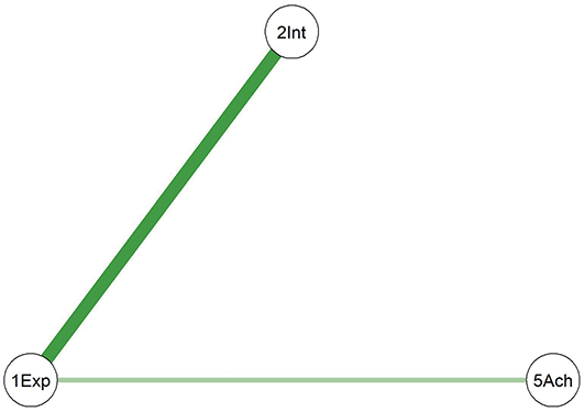
Partial network that examines the relations among intrinsic value, Prior achievement, and attainment value (2Int-5Ach-3AtV) using psychological network analysis.

Partial network that examines the relations among intrinsic value, prior achievement, and utility value (2Int-5Ach-4UtV) using psychological network analysis.

# Fitting partial correlation networks for selected variable combinations# Fit for Intrinsic Value, Prior Achievement, and Expectancy for Success (2Int-5Ach-1Exp)fit.251 <- mgm( dag_demo_FS[, c(2, 5, 1)], type = rep(‘g‘, 3), lambdaSeq = 0, lambdaSel = "EBIC" # Gaussian variables with EBIC selection)Labels <- c("2Int", "5Ach", "1Exp")qgraph( fit.251$pairwise$wadj, threshold = 0.15, labels = Labels, title = "Intrinsic Value, Prior Achievement, and Expectancy for Success")
# Fit for Intrinsic Value, Prior Achievement, and Attainment Value (2Int-5Ach-3Atv)fit.253 <- mgm( dag_demo_FS[, c(2, 5, 3)], type = rep(‘g‘, 3), lambdaSeq = 0, lambdaSel = "EBIC" # Gaussian variables with EBIC selection)Labels <- c("2Int", "5Ach", "3AtV")qgraph( fit.253$pairwise$wadj, threshold = 0.15, labels = Labels, title = "Intrinsic Value, Prior Achievement, and Attainment Value")
# Fit for Intrinsic Value, Prior Achievement, and Utility Value (2Int-5Ach-4UtV)fit.254 <- mgm( dag_demo_FS[, c(2, 5, 4)], type = rep(‘g‘, 3), lambdaSeq = 0, lambdaSel = "EBIC" # Gaussian variables with EBIC selection)Labels <- c("2Int", "5Ach", "4Utv")qgraph( fit.254$pairwise$wadj, threshold = 0.15, labels = Labels, title = "Intrinsic Value, Prior Achievement, and Utility Value")
Similar to the previous analysis, based on the disappearance of another pairwise connection in the partial correlation network (2Int-5Ach), we applied the ICA to examine how this connection interacted with other nodes in different combinations within the partial correlation networks. We found that the link between intrinsic value and prior achievement disappeared when expectancy for success was present (refer to Figure 21). Therefore, we inferred that there could be a collider effect where both intrinsic value and prior achievement pointed to expectancy for success (2Int → 1Exp ←5Ach). There was no need to examine the relations between four variables (e.g., 2Int-5Ach-1Exp-3AtV or 2Int-5Ach1Exp-4UtV or 2Int-5Ach-3AtV-4UtV) because we already directed the lines.
Now that the directionality of effects between interest value and prior achievement was depicted, we examined the partial correlation network to seek further possible directed lines. We found that the association between expectancy for success and utility value as well as expectancy for success and attainment value was still missing (or non-directed) in our directed acyclic graph. So, we started with the association between expectancy for success and utility value. We first tried pointing utility value to expectancy for success. However, this option was not possible because there should have been a zero-order correlation between utility value and prior achievement due to a common effect. So, the only other option was to point expectancy for success to utility value. Next, we examined the association between expectancy for success and attainment value. We first tried pointing attainment value to expectancy for success. But this was not a possible option for the directed acyclic graph because then there was a cyclical relation among attainment value, expectancy for success, and utility value (i.e., 3AtV → 1Exp → 4UtV →3AtV), which meant the graph was not acyclic anymore. So, the only other option was to point expectancy for success to attainment value.
As a result, we ended up with Figure 24. The following lines were directed: both prior achievement and intrinsic value pointed to expectancy for success, both intrinsic value and utility value pointed to attainment value, and expectancy for success both pointed to utility value and attainment value.
Directed network diagram of the five SEVT variables finally derived using psychological network analysis and ICA. (Note: Exp represents Expectancies, InV represents Intrinsic Value, AtV represents Attainment Value, Utv represents Utility Value, and Ach represents Achievement.)
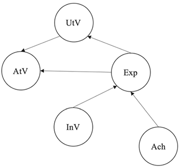
In summary, we selected three variables at a time to search for conditional independence between a pair. The ICA provides outputs of partial correlations among the three variables along with a visual undirected graph. Using this output, we ascertain the direction by examining the undirected graph and comparing zero-order correlations with partial correlations. The relation is deemed a chain if there is no significant difference between zero-order and partial correlations. Conversely, the relation is classified as either a confound or a collider if there is a significant difference. Once we establish the directionality among these three variables, we repeat this process with other variables until the directed acyclic graphs are complete. It is important to note that the ICA does not provide a definitive answer but offers multiple plausible directed acyclic graphs.
7 Discussion
This Element has presented a step-by-step introduction to psychological network analysis and demonstrated its methodological contributions to developmental and educational sciences. Rather than focusing on specific empirical findings, our goal was to show how different types of psychological networks can be constructed, interpreted, and applied to address key questions in these fields. Through three illustrative case studies, we highlighted how psychological network analysis techniques offer distinctive analytical value that complements – and in some cases surpasses – traditional statistical models.
In the first case study, we demonstrated how undirected networks can be used to explore the conditional structure among psychological variables, allowing researchers to visualize and quantify how traits co-occur while controlling for other factors. This modeling approach is particularly useful for identifying central variables, detecting differences across groups, and revealing latent patterns that are not easily captured by conventional latent variable models. By applying this framework to cross-sectional and cohort data, we also introduced techniques such as network comparison and centrality analysis, which support nuanced understanding of group differences and developmental trends.
The second case study showcased longitudinal network analysis, which provides a dynamic perspective on how psychological variables evolve over time. Through temporal, contemporaneous, and between-subject networks, this framework allows researchers to disentangle autoregressive stability, moment-to-moment covariation, and population-level structures within the same dataset. These methods are especially powerful for capturing within-person processes, identifying feedback mechanisms, and detecting sensitive periods for developmental change – challenges that often go unmet in traditional panel models.
In the third case study, we introduced directed acyclic graph as a tool for exploring potential causal structures in cross-sectional data. Although directed acyclic graphs do not provide definitive causal claims, they offer a principled way to generate and test causally plausible hypotheses using algorithmic rules and conditional independence tests. This enables researchers to reason about causal directionality across multiple variables simultaneously – an advantage over more restrictive models like CLPM or SEM, which often require predefined structures and struggle with omitted variable bias.
Together, these case studies underscore how psychological network analysis supports a more transparent, flexible, and exploratory approach to modeling psychological systems – particularly those characterized by complexity, context sensitivity, and developmental change. In the following sections (7.1–7.3), we elaborate on the specific applications, limitations, and broader significance of psychological network analysis in developmental and educational research.
7.1 Application and Value of Psychological Network Analysis in Developmental Psychology
7.1.1 Dynamic Perspective: Unveiling the Temporal Evolution and Developmental Trajectories of Psychological Systems
Developmental science emphasizes the dynamic changes in individuals’ psychological systems over time (Molenaar & Nesselroade, Reference Martin and Lazendic2015; van Geert & Steenbeek, Reference van Borkulo, van Bork and Boschloo2005). Psychological network analysis makes this dynamicity tangible. For instance, comparing networks across different age groups allows researchers to observe how relations between psychological variables evolve over time. In this Element, we demonstrated such differences between young adults (18–30 years) and middle-aged adults (31–60 years): The positive relation between extraversion and conscientiousness was prominent in the younger group but gradually weakened in the middle-aged group. This shift may suggest that in younger individuals, extraverted social activities align closely with a sense of responsibility, whereas in middle adulthood, improved emotional regulation may replace such direct associations with more complex influences.
Furthermore, longitudinal network analysis can trace how variables change and interact over time (Epskamp, Waldorp, et al., Reference Epskamp, Waldorp, Mõttus and Borsboom2018; Panayiotou et al., Reference Neal and Neal2023). For example, the feedback loop between positive affect and self-confidence indicates that positive emotional experiences not only enhance individuals’ self-efficacy but also reinforce a stable state of positive emotions. This finding has significant implications for identifying critical intervention points in developmental psychology. Specifically, during childhood and adolescence, fostering positive emotional experiences may facilitate the formation of a virtuous developmental trajectory, helping individuals navigate challenges in learning and life effectively (Larson, Reference Kwiatkowski, Phillips, Schmidt and Shin2000).
7.1.2 Holistic Perspective: Capturing Complex Relations with Psychological Networks
In developmental and educational science, understanding the complex interactions between variables is essential. Traditional latent variable models, such as structural equation modeling, aggregate multiple observed variables into abstract latent constructs and infer relations between these constructs through predefined pathways. However, this approach can obscure the direct relations between observed variables and assumes linear, unidirectional associations, which may not fully capture the nonlinear and highly interconnected nature of psychological systems (Borsboom, Reference Borsboom2022; Borsboom & Cramer, Reference Borsboom and Cramer2013). In contrast, psychological network analysis directly incorporates individual items as nodes and visually represents the independent relations and interaction patterns among variables (Borsboom, Deserno, et al., Reference Borsboom, van der Maas, Kievit and Haig2021; Costantini et al., Reference Costantini, Epskamp and Borsboom2015). This approach preserves the complexity and realism of variable interactions without assuming the existence of latent constructs.
More importantly, psychological network analysis retains the intricate interaction patterns among variables. By analyzing the network structure, researchers can observe the independent associations between variables after controlling for others, offering new theoretical insights and practical applications (Epskamp, Borsboom, et al., Reference Epskamp, van Borkulo and van der Veen2018; Epskamp & Fried, Reference Epskamp and Fried2018). Unlike SEM, which emphasizes commonalities, psychological network analysis highlights the uniqueness and independence of relations, preserving the richness and diversity of data (Abacioglu et al., Reference Abacioglu, Isvoranu, Verkuyten, Thijs and Epskamp2019).
7.1.3 Exploratory Strength: Advancing Theoretical Innovation and Practical Applications
Traditional theory-testing research often relies on predefined frameworks, limiting its flexibility in uncovering unexpected relations between variables (Abacioglu et al., Reference Abacioglu, Isvoranu, Verkuyten, Thijs and Epskamp2019; Borsboom, Deserno, et al., Reference Borsboom, Deserno and Rhemtulla2021). In contrast, the exploratory strength of psychological network analysis allows researchers to identify potential associations, fostering theoretical innovation and development (Borsboom, Reference Borsboom2022; Samra et al., Reference Rohrer2023; Tao et al., Reference Tang, Renninger, Hidi, Murayama, Lavonen and Salmela-Aro2023). For example, in longitudinal network analysis, this Element demonstrated how positive affect and confidence form a feedback loop over time, where increases in positive emotions enhance confidence, and greater confidence, in turn, reinforces positive emotions. This highlights the evolving interplay between emotions and self-perception, providing insights into how psychological states stabilize or change across different developmental stages. Such exploratory findings provide researchers with novel perspectives, encouraging deeper investigations into previously overlooked psychological processes.
This exploratory strength is particularly valuable in developmental science, where many research areas remain underexplored. For instance, studies on adolescent psychological development may uncover “weak connections” between variables – subtle yet stable relations that could serve as critical turning points in an individual’s psychological trajectory. These discoveries not only offer robust support for future theoretical and empirical studies but also inspire researchers to design more targeted and effective educational interventions in practice.
7.1.4 Efficient Exploration of Causal Pathways: The Application of Directed Acyclic Graphs
Identifying causal relations is a central goal in developmental and educational sciences. However, experimental or longitudinal designs – though rigorous – often involve substantial logistical, ethical, and financial constraints, especially in real-world educational settings (Borsboom & Cramer, Reference Borsboom and Cramer2013; Lee et al., Reference Larson2024). Directed acyclic graphs offer a more accessible and efficient alternative by enabling researchers to explore plausible causal structures using existing observational data.
The cost-effectiveness does not lie in the mere use of cross-sectional data, but in the ability of directed acyclic graphs to extract causal hypotheses from such data through rigorous algorithmic procedures grounded in conditional independence theory. Though the resulting models are inherently exploratory and require further validation, they provide a structured, theory-informed foundation for future confirmatory work – be it longitudinal or experimental.
For example, a directed acyclic graph analysis might suggest that enhancing students’ intrinsic value (e.g., interest and enjoyment) could indirectly boost academic performance. These insights help researchers prioritize key variables and pathways for intervention, especially when resources for large-scale causal studies are limited. In this way, directed acyclic graphs serve as a valuable preliminary tool for theory-building and practical decision-making in complex educational environments.
7.2 Limitations of Psychological Network Analysis
Though psychological network analysis provides a powerful tool for developmental and educational sciences, it also presents certain limitations that require careful consideration.
First, psychological network analysis is highly dependent on sample size, which poses a significant challenge (Epskamp & Fried, Reference Epskamp and Fried2018; Isvoranu & Epskamp, 2023). The stability and accuracy of network models rely on sufficient sample sizes, especially in high-dimensional networks with a large number of nodes (Epskamp, Borsboom, et al., Reference Epskamp, Borsboom and Fried2018).
Though no universal rule fits all scenarios, several empirical guidelines and simulation-based studies can help researchers approximate sample size requirements. For example, simulation studies suggest that for networks with up to thirty nodes, a sample size of at least several hundred participants is necessary to achieve stable and interpretable results. In scenarios where the network includes a larger number of nodes or when the research focuses on detecting weaker connections (e.g., bridge edges), larger sample sizes – potentially exceeding 1,000 participants – may be required to ensure adequate statistical power and reliability of the findings (Isvoranu & Epskamp, 2023; Isvoranu et al., Reference Isvoranu and Epskamp2022).For centrality indices, which are more sensitive to sampling variability, even larger sample sizes may be necessary to ensure reliable rank ordering (Bringmann et al., Reference Bringmann, Elmer and Epskamp2019). In the context of longitudinal networks, such as those estimated via mlVAR, the number of measurement occasions per participant (e.g., time points ≥ 30) is often more influential than the number of participants per se (Epskamp, Reference Epskamp2020; Epskamp, Waldorp, et al., Reference Epskamp, Waldorp, Mõttus and Borsboom2018).
Post hoc analyses are equally important in assessing the robustness of network models. Techniques such as bootstrapping can be employed to evaluate the stability of network parameters, including edge weights and centrality measures. For instance, the bootnet package in R provides bootstrap-based accuracy analyses that can be used post hoc to assess whether the obtained network estimates are robust given the sample size, and the correlation stability coefficient (CS-coefficient) can be calculated to determine the reliability of centrality indices, with higher values indicating greater stability.
To assist researchers in planning and evaluating their studies, tools like the netSimulator function from the bootnet R package have been developed. This function allows researchers to conduct simulation studies by varying sample sizes and network structures, thereby providing empirical guidance on the sample size needed for their specific research context. By inputting an expected network structure, researchers can assess how different sample sizes impact the accuracy and stability of the estimated networks, facilitating informed decision-making during the study design phase.
Sample size concern is particularly salient when studying populations with limited data availability – such as young children, special education samples, or individuals with rare developmental disorders – where recruitment is challenging. In these cases, researchers are encouraged to (a) reduce the number of nodes by aggregating indicators or using theoretically driven variable selection, (b) employ regularization-based modeling approaches (e.g., graphical LASSO), and (c) conduct robustness checks using bootstrapped accuracy intervals and network comparison tests.
Second, results overinterpretation should be cautioned. Although psychological network analysis’s exploratory nature allows for the identification of novel associations between variables (Borsboom, Reference Borsboom2022), it also increases the risk of noise-driven or overinterpreted relations (Epskamp & Fried, Reference Epskamp and Fried2018; Lee et al., Reference Larson2024). Therefore, psychological network analysis must be integrated with existing theoretical frameworks to enhance validity.
Third, the choice of modeling methods may impact result interpretation (Epskamp, Borsboom, et al., Reference Epskamp, Borsboom and Fried2018; Isvoranu & Epskamp, 2023). For instance, longitudinal network analysis assumes temporal stationarity and equal time intervals between measurements, conditions that are often difficult to achieve in real-world data collection. Non-stationary or irregularly spaced data may require complex preprocessing, such as detrending, which involves identifying and removing long-term systematic changes or trends from time series data. It aims to render data stationary, satisfying the fundamental assumption of subsequent statistical models (e.g., VAR models). Failure to detrend non-stationary data can lead to spurious correlations, inaccurate estimations, and unreliable causal inferences. Similarly, directed acyclic graphs rely on strong assumptions for causal inference, such as the absence of unmeasured confounding variables. These assumptions may oversimplify the model or fail to fully capture the complexity of real-world causal relations (Lee et al., Reference Larson2024).
7.3 Contributions of Psychological Network Analysis
Despite some caveats, psychological network analysis still holds significant potential to play a more central role in developmental and educational science, advancing both theoretical innovation and practical applications.
First, psychological network analysis contributes to advancing theoretical innovation in developmental and educational science by uncovering complex, data-driven relations that traditional models may overlook. Psychological network analysis can offer new pathways for theory development (Borsboom, Reference Borsboom2022). By employing network models, researchers can uncover complex relations among variables that traditional latent variable models may overlook, and even identify new key nodes or mechanisms. For example, in longitudinal network analysis, the centrality of certain variables – such as self-concept or emotional regulation – may change significantly at critical developmental stages, providing evidence for identifying developmental turning points. Coupled with directed acyclic graphs, researchers can establish data-driven causal hypotheses and verify dynamic causal chains between variables. This integration of exploratory and confirmatory approaches will enhance and refine theoretical frameworks in developmental psychology.
Second, psychological network analysis supports the optimization of individualized intervention strategies by identifying key variables and pathways that can be targeted for personalized educational or psychological support. Insights gained from psychological network analysis allow researchers to identify key variables and connections within dynamic relations, providing a solid foundation for designing targeted interventions (Borsboom & Cramer, Reference Borsboom and Cramer2013). For example, in educational psychology, if a network reveals that “self-efficacy” serves as a bridging node at a specific developmental stage, interventions targeting this node may be particularly effective. In this Element, longitudinal network analysis revealed the feedback mechanism between positive emotions and confidence. Such dynamic relations provide theoretical support for the design of interventions aimed at improving emotional management and fostering motivation.
Third, psychological network analysis enables cross-level comparative research by allowing researchers to systematically examine how psychological structures differ across age groups, cultures, or contexts using formal network comparison methods. The network comparison techniques used in psychological network analysis (e.g., structure and edge difference tests) offer powerful tools for cross-level studies in developmental psychology, helping to identify key differences across age groups, cultures, or populations (Abacioglu et al., Reference Abacioglu, Isvoranu, Verkuyten, Thijs and Epskamp2019; Tao et al., Reference Tang, Renninger, Hidi, Murayama, Lavonen and Salmela-Aro2023; van Borkulo et al., Reference Thissen, Steinberg and Kuang2023). Future cross-cultural comparisons and group difference analyses will further elucidate the mechanisms through which external contextual factors shape psychological networks, offering insights for universal theories and localized practices.
8 Conclusion
This Element has provided a comprehensive exploration of psychological network analysis and its applications in developmental and educational sciences. The significance of psychological network analysis lies in its ability to provide a systematic and nuanced understanding of the interrelations among psychological constructs. Unlike traditional statistical methods that often isolate variables, psychological network analysis considers their interdependencies, enabling researchers to visualize and interpret the dynamics within a system. This capability is especially valuable in developmental and educational sciences, where variables often interact in intricate and context-specific ways.
Through undirected networks, psychological network analysis has demonstrated its strength in uncovering latent structures and identifying clusters of closely related variables, offering actionable insights for interventions. The application of longitudinal networks extends this understanding by revealing how relations evolve over time, making it possible to detect critical periods for developmental and educational interventions. Meanwhile, directed acyclic graphs serve as a bridge between exploratory and confirmatory methodologies, allowing researchers to generate testable hypotheses about causal relations.
As an analytical approach, psychological network analysis offers a promising path toward integrating exploratory insights with formalized causal models. This integrative capacity positions psychological network analysis as a pivotal tool for addressing long-standing challenges in psychological research, such as the need for testable hypotheses, robust theoretical frameworks, and personalized interventions.
The adoption of psychological network analysis in psychological and educational research reflects an ongoing shift toward more holistic and dynamic methodologies. By capturing the complex interplay of variables and integrating cross-sectional, longitudinal, and causal perspectives, psychological network analysis aligns with the increasing demand for nuanced and context-sensitive analyses. Its flexibility allows researchers to adapt the method to a wide range of datasets and research designs, from large-scale surveys to intensive longitudinal assessments.
Brett Laursen
Florida Atlantic University
Brett Laursen is a Professor of Psychology at Florida Atlantic University. He is Editor-in-Chief of the International Journal of Behavioral Development, where he previously served as the founding Editor of the Methods and Measures section. Professor Laursen received his Ph.D. in Child Psychology from the Institute of Child Development at the University of Minnesota and an Honorary Doctorate from Örebro University, Sweden. He is a Docent Professor of Educational Psychology at the University of Helsinki, and a Fellow of the American Psychological Association (Division 7, Developmental), the Association for Psychological Science, and the International Society for the Study of Behavioural Development. Professor Laursen is the co-editor of the Handbook of Developmental Research Methods and the Handbook of Peer Interactions, Relationships, and Groups.
About the Series
Each offering in this series will focus on methodological innovations and contemporary strategies to assess adjustment and measure change, empowering scholars of developmental science who seek to optimally match their research questions to pioneering methods and quantitative analyses.