





Introduction
Designing is regarded as a means of changing existing situations into preferred ones. The engineering design process has been broadly classified into four stages: task clarification, conceptual design, embodiment design, and detail design (Pahl and Beitz, Reference Pahl and Beitz1996). Conceptual design is an early stage in the design process, which involves generating solution concepts to satisfy the functional requirements of a design problem (Chakrabarti and Bligh, Reference Chakrabarti and Bligh1994). The conceptual design stage is crucial because a high percentage of the product cost is committed at this stage (Saravi et al., Reference Saravi, Newnes, Mileham and Goh2008). Decisions made during this stage will strongly affect all the subsequent stages of the design process. Past research (Baer, Reference Baer2014) relates creativity to “divergent thinking,” i.e., how well the concept space is explored during the early phase of design. The ability to explore the breadth of the concept space is directly related to the ability to restructure problems and is, therefore, an important measure of creativity in design (Shah et al., Reference Shah, Smith and Vargas-Hernandez2003). Concept space exploration depends on the capacity to produce a wider “variety” of ideas with higher “fluency” (Shah et al., Reference Shah, Smith and Vargas-Hernandez2003). Researchers (Chakrabarti and Bligh, Reference Chakrabarti and Bligh1994; Shah et al., Reference Shah, Smith and Vargas-Hernandez2003) have argued that generating several concepts would increase the chances of producing better design solutions, a view that aligns with Osborn’s (Reference Osborn2012) foundational brainstorming principle that “quantity breeds quality,” whereby generating many ideas enhances the chances of arriving at more effective and innovative solutions. Past empirical studies also showed that the variety of the concept space is positively correlated with the novelty of the generated set of ideas (Kurtoglu et al., Reference Kurtoglu, Campbell and Linsey2009; Srinivasan and Chakrabarti, Reference Srinivasan and Chakrabarti2010a; Jagtap et al., Reference Jagtap, Larsson, Hiort, Olander and Warell2015). Generating many concepts, resulting in higher “fluency” (i.e., the total count of the number of concepts generated), that differ from one another only in minor or superficial ways does not prove effective in concept generation (Shah et al., Reference Shah, Smith and Vargas-Hernandez2003). Here, minor or superficial ways refer to differences that do not meaningfully alter the functional, behavioral, or structural aspects of a design concept, for example, changing the color, naming, or trivial features while maintaining essentially the same underlying principles. Thus, it is imperative to generate and explore a diverse set of alternative solution concepts during the early stages of the design process. This approach ensures that designers have a multitude of options to consider, which increases the likelihood that designers can identify and pursue a promising solution.
Variety indicates how well one has explored the concept space of a design problem. Variety metrics, often referred to as “diversity” metrics, are also popular in other domains such as economics and ecology. Mathematically, a variety or diversity measure should tell us the probability that two objects (or species – in the case of ecology) selected at random (without replacement) from a sample will belong to different groups (Hurlbert, Reference Hurlbert1971; Ahmed et al., Reference Ahmed, Ramachandran, Fuge, Hunter and Miller2021).
Other than evaluating concept generation, assessing variety also offers value in design-by-analogy, where designers are presented with external stimuli to inspire new ideas. Prior research has shown that the diversity of stimuli – often captured as the conceptual “distance” between the target design problem and the analogical sources – substantially influences the ideation process, affecting the originality or novelty of resulting concepts (Gonçalves et al., Reference Gonçalves, Cardoso and Badke-Schaub2012; Lu et al., Reference Lu, Sun, Xu, Su, Tang and Zhang2023). Therefore, having a computational method to quantify variety becomes useful not only for evaluating concept sets but also for systematically selecting and presenting diverse stimuli to designers, ensuring exposure to analogies that span a broad conceptual range.
This article critically examines the existing variety metrics from the engineering design literature and highlights the limitations of the existing metrics through test cases. Specifically, existing metrics rely on a genealogy tree-based representation of concept space, which assumes that concepts can always be classified into discrete nodes at predefined abstraction levels (physical principle, working principle, embodiment, and detail). This binary, node-based approach limits flexibility, especially when real-valued distances – such as semantic similarity scores – are more appropriate for capturing the relationship between ideas generated at a particular abstraction level, making current metrics unsuitable for such scenarios. Furthermore, some existing metrics demonstrate a lack of accuracy and sensitivity in special test cases, ultimately leading to misleading variety scores that do not adhere to the mathematical definition of variety. Additionally, so far, no software tools are reported in the literature that can automate the variety assessment process directly from textual data of a design concept space. Finally, researchers often report difficulties in clearly defining physical and working principles during genealogy tree creation, indicating a need for a more flexible and robust framework that can accommodate customizable abstraction levels tailored to different design problems. To address these limitations, a new variety metric is proposed based on Rao’s quadratic diversity index (Rao, Reference Rao1982), along with a prescriptive framework – embodied into a software tool – to support the assessment process. The proposed metric offers advantages over the existing variety metrics as it eliminates the need for a tree-like representation of a design concept space. This framework uses automated text-to-vector embedding to measure the real-valued distance between two design concepts across the distinct levels of abstraction. Although the example implementation of the proposed framework uses a particular abstraction scheme, the framework itself is generalizable and can accommodate any representation of abstraction and any distance-assessment method, allowing designers the flexibility to define abstraction levels that best suit their specific design context. The framework is implemented in a software tool called “VariAnT.” The general applicability of the proposed framework is demonstrated through multiple examples.
Background and related work
This section reviews existing metrics for measuring the variety of a concept space proposed in the engineering design domain. To elaborate on these metrics, Section “An example concept space and its genealogy tree” first introduces an example concept space, followed by the construction of its genealogy tree. Then, in Section “Existing variety metrics in engineering design,” we use this genealogy tree to explain the existing variety metrics in detail.
An example concept space and its genealogy tree
At the conceptual design stage, a designer moves freely between different levels of abstraction and generates ideas corresponding to a particular abstraction level (Srinivasan and Chakrabarti, Reference Srinivasan and Chakrabarti2010b). Most of the existing literature on variety considers four abstraction levels: physical principle, working principle, embodiment, and detail (Shah et al., Reference Shah, Smith and Vargas-Hernandez2003; Nelson et al., Reference Nelson, Wilson, Rosen and Yen2009; Verhaegen et al., Reference Verhaegen, Vandevenne, Peeters and Duflou2013; Henderson et al., Reference Henderson, Helm, Jablokow, McKilligan, Daly and Silk2017; Ahmed et al., Reference Ahmed, Ramachandran, Fuge, Hunter and Miller2021). Let us consider an example case illustrated in Figure 1, where a designer explores ideas with an AI chatbot to fulfil the function of “pumping water.” The chatbot provided two ideas at the physical principle level: “centrifugal force” and “positive displacement.” Now, based on these two physical principles, five concepts are generated, each representing a distinct idea at the working principle level. The exploration can go further at the embodiment and detail level, which may lead to a concept space
$ \mathrm{C}=\left\{{\mathrm{C}}_1,{\mathrm{C}}_2,\dots, {\mathrm{C}}_{\mathrm{N}}\right\} $
 with
$ N $
with
$ N $
 number of concepts where each can be represented in
$ \alpha $
number of concepts where each can be represented in
$ \alpha $
 levels of abstraction. For convenience, we have only represented the concepts at two levels of abstraction: physical principle (
$ \alpha =1 $
levels of abstraction. For convenience, we have only represented the concepts at two levels of abstraction: physical principle (
$ \alpha =1 $
 ) and working principle (
$ \alpha =2 $
) and working principle (
$ \alpha =2 $
 ). At each
$ \alpha $
). At each
$ \alpha $
 , there exists a different set of ideas,
$ {I}^{\alpha }=\left\{{I}_i^{\alpha}\hskip0.5em \mid \hskip0.5em i\in 1,2,\dots, {\beta}_{\alpha}\right\} $
, there exists a different set of ideas,
$ {I}^{\alpha }=\left\{{I}_i^{\alpha}\hskip0.5em \mid \hskip0.5em i\in 1,2,\dots, {\beta}_{\alpha}\right\} $
 , where
$ {\beta}_{\alpha } $
, where
$ {\beta}_{\alpha } $
 denotes a total number of ideas at
$ \alpha $
denotes a total number of ideas at
$ \alpha $
 . Therefore, a concept
$ {C}_i $
. Therefore, a concept
$ {C}_i $
 can be generated by combining different ideas taken from the idea space
$ {I}^{\alpha } $
can be generated by combining different ideas taken from the idea space
$ {I}^{\alpha } $
 , as shown in Figure 1. We refer to the concept space shown in Figure 1 as
$ {C}^A $
, as shown in Figure 1. We refer to the concept space shown in Figure 1 as
$ {C}^A $
 where
$ N=5 $
where
$ N=5 $
 .
.
Concept space (
$ {C}^A $
 ) generated by combining different ideas from different levels of abstraction.

Figure 1. Long description
The flowchart is divided into three horizontal layers separated by dashed lines, with a legend on the right and a definition box at the bottom.
1. Top Layer (Function): A yellow box at the top center labeled To pump water. Two arrows branch downward from this box.
2. Middle Layer (Physical principle alpha = 1): Two red boxes. The left box is labeled I sub 1 super 1 Centrifugal Force. The right box is labeled I sub 2 super 1 Positive Displacement.
3. Bottom Layer (Working principle alpha = 2): Five green boxes containing detailed technical descriptions.
- Branching from Centrifugal Force are two boxes: I sub 1 super 2 describes utilizing a diffuser and stationary component to convert kinetic energy; I sub 2 super 2 describes plunging the pump unit underwater with a motor shaft impeller.
- Branching from Positive Displacement are three boxes: I sub 3 super 2 describes rollers or shoes compressing a flexible tube; I sub 4 super 2 describes rotating screws or helical rotors; I sub 5 super 2 describes rotating lobes inside a casing.
4. Bottom Definition Box: Contains the mathematical set notation Concept C sub i = I sub j super 1 union I sub k super 2. It provides an example for a Screw pump where C sub 4 = I sub 2 super 1 union I sub 4 super 2, explaining that it combines the physical principle of positive displacement with the working principle of rotating helical screws.
Design concepts and the corresponding SAPPhIRE models generated with the help of ChatGPT (GPT-4o)

Table 1. Long description
The table consists of five columns and eight rows. The first column lists the S A P P h I R E model abstraction levels, while columns two through five describe four concepts: Electric kettle, Gas stove with kettle, Solar water heater, and Friction heater.
* Actions: Concepts 1, 2, and 3 involve boiling of water. Concept 4 involves water becoming warm.
* (change of) States: Concepts 1, 2, and 3 move from cold water (low temperature) to hot water (high temperature). Concept 4 moves from cool water (moderate temperature) to warm water (higher temperature).
* Phenomena: Concept 1 uses electrical to heat energy conversion. Concept 2 uses gas combustion and heat transfer from flame to kettle to water. Concept 3 uses solar to heat energy conversion. Concept 4 uses mechanical to heat energy conversion via friction.
* Effects: Concept 1 uses Joule heating and conduction. Concept 2 uses chemical reaction and conduction. Concept 3 uses photovoltaic effect and heat transfer. Concept 4 uses frictional heating.
* Inputs: Concept 1 requires electrical energy. Concept 2 requires natural gas. Concept 3 requires solar energy. Concept 4 requires mechanical energy from manual rotation.
* o R gans: Lists structural requirements such as conductive materials for Concept 1, combustible gas and metallic kettles for Concept 2, photovoltaic cells and insulated tanks for Concept 3, and high-friction rods with smooth bearings for Concept 4.
* Parts: Lists physical components like heating elements (Concept 1), gas burners (Concept 2), solar panels (Concept 3), and friction rods with crank handles (Concept 4).
Design concepts partially taken from Henderson et al. (Reference Henderson, Helm, Jablokow, McKilligan, Daly and Silk2017)
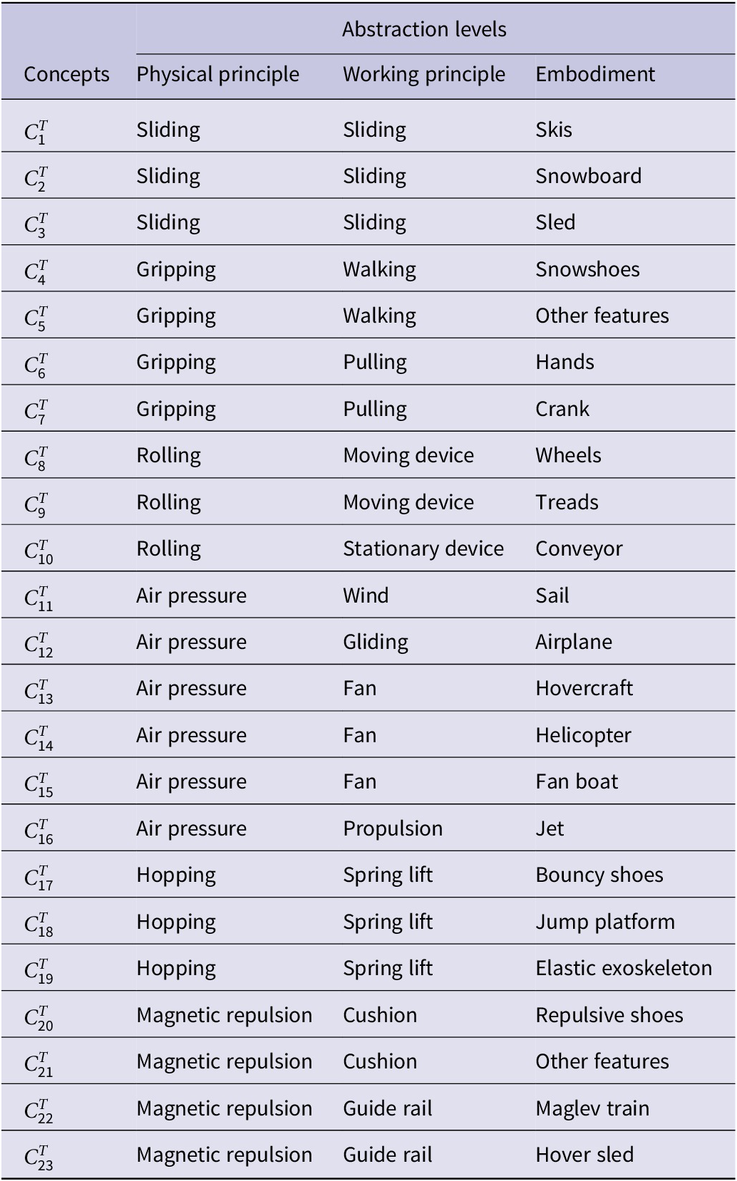
Table 2. Long description
The table consists of four columns: Concepts, Physical principle, Working principle, and Embodiment. It lists 23 concepts labeled C sub 1 super T through C sub 23 super T.
* Concepts C sub 1 super T to C sub 3 super T: Physical principle is Sliding, Working principle is Sliding, Embodiments are Skis, Snowboard, and Sled.
* Concepts C sub 4 super T to C sub 7 super T: Physical principle is Gripping. Working principles include Walking (Snowshoes, Other features) and Pulling (Hands, Crank).
* Concepts C sub 8 super T to C sub 10 super T: Physical principle is Rolling. Working principles include Moving device (Wheels, Treads) and Stationary device (Conveyor).
* Concepts C sub 11 super T to C sub 16 super T: Physical principle is Air pressure. Working principles include Wind (Sail), Gliding (Airplane), Fan (Hovercraft, Helicopter, Fan boat), and Propulsion (Jet).
* Concepts C sub 17 super T to C sub 19 super T: Physical principle is Hopping, Working principle is Spring lift, Embodiments are Bouncy shoes, Jump platform, and Elastic exoskeleton.
* Concepts C sub 20 super T to C sub 23 super T: Physical principle is Magnetic repulsion. Working principles include Cushion (Repulsive shoes, Other features) and Guide rail (Maglev train, Hover sled).
In most of the literature on variety assessment, researchers have used a tree-like structure, called a genealogy tree, to represent a concept space. For example, Figure 2 illustrates the genealogy tree of concept space,
$ {C}^A $
 . Here,
$ {n}_i^{\alpha } $
. Here,
$ {n}_i^{\alpha } $
 denotes the total number of concepts that use the
$ {i}^{th} $
denotes the total number of concepts that use the
$ {i}^{th} $
 idea from the idea space
$ {I}^{\alpha } $
idea from the idea space
$ {I}^{\alpha } $
 . If
$ {\beta}_{\alpha } $
. If
$ {\beta}_{\alpha } $
 is the maximum number of ideas in
$ {I}^{\alpha } $
is the maximum number of ideas in
$ {I}^{\alpha } $
 , then we can write,
$ {\sum}_{i=1}^{\beta_{\alpha }}{n}_i^{\alpha }=N $
, then we can write,
$ {\sum}_{i=1}^{\beta_{\alpha }}{n}_i^{\alpha }=N $
 . It is important to note that even if we describe the concept space
$ {C}^A $
. It is important to note that even if we describe the concept space
$ {C}^A $
 at the embodiment and detail abstraction level, the genealogy tree will still have 5 nodes at those lower hierarchical levels, with each node containing one idea, and hence, the variety score at the embodiment and detail level will be the same as the working principle level, irrespective of the existing variety metrics (elaborated in Section “Existing variety metrics in engineering design”) that we use. Hence, using the concept space
$ {C}^A $
at the embodiment and detail abstraction level, the genealogy tree will still have 5 nodes at those lower hierarchical levels, with each node containing one idea, and hence, the variety score at the embodiment and detail level will be the same as the working principle level, irrespective of the existing variety metrics (elaborated in Section “Existing variety metrics in engineering design”) that we use. Hence, using the concept space
$ {C}^A $
 and its corresponding tree as a common ground, we have elaborated on the existing variety assessment techniques in the following part of this section.
Tree constructed from concept space
$ {C}^A $
 .
.

Figure 2. Long description
The tree diagram is organized into three horizontal levels connected by solid lines.
* At the top level, a single box is labeled N = 5. A dashed line to the left identifies this as Total number of concepts.
* The second level down is labeled Physical principle, alpha = 1. It contains two boxes branching from the top node. The left box is labeled n sub 1 super 1 = 2. The right box is labeled n sub 2 super 1 = 3.
* The third and bottom level is labeled Working principle, alpha = 2. It contains five boxes. Two boxes branch from the left node of the second level, labeled n sub 1 super 2 = 1 and n sub 2 super 2 = 1. Three boxes branch from the right node of the second level, labeled n sub 3 super 2 = 1, n sub 4 super 2 = 1, and n sub 5 super 2 = 1.
Existing variety metrics in engineering design
In engineering design, there are two commonly used approaches to assess design variety: subjective ratings and objective ratings. As an example of subjective evaluation, Linsey et al. (Reference Linsey, Clauss, Kurtoglu, Murphy, Wood and Markman2011) proposed a method where a coder intuitively categorizes design concepts based on their overall differences. Concepts with similar features are sorted into different bins or pools. At the end of the sorting process, an individual’s variety score is calculated as the ratio of the number of bins the concepts were sorted into to the total number of bins. This subjective approach relies on the coder’s mental model rather than a numerical procedure (Ahmed et al., Reference Ahmed, Ramachandran, Fuge, Hunter and Miller2021). In contrast, the objective approaches replace subjective human raters with a deterministic formula that relies on a few measured attributes of a set of designs. Our work particularly focuses on objective approaches. Here, we have reviewed four existing objective variety metrics related to the engineering design domain: the variety metrics proposed by Shah et al. (Reference Shah, Smith and Vargas-Hernandez2003), Nelson et al. (Reference Nelson, Wilson, Rosen and Yen2009), Verhaegen et al. (Reference Verhaegen, Vandevenne, Peeters and Duflou2013), and Ahmed et al. (Reference Ahmed, Ramachandran, Fuge, Hunter and Miller2021). Note that other objective variety metrics also do exist in engineering design literature, but we kept those out of our discussion for the following reasons: (a) for example, the metric proposed by Henderson et al. (Reference Henderson, Helm, Jablokow, McKilligan, Daly and Silk2017) uses other design assessment metrics, such as quality, effectiveness, novelty, applicability, and so forth, to calculate the variety of the solution concepts and thus, the variety metric cannot be considered as an independent measure; (b) in case of the metric proposed by Srinivasan and Chakrabarti (Reference Srinivasan and Chakrabarti2009), the measure is dependent on the order in which the ideas are generated, even though this should not have any impact on the overall variety of a concept space as long as it contains the same set of concepts, and hence the metric is not applicable for the concept space
$ {C}^A $
 .
.
Metric proposed by Shah
Shah et al. (Reference Shah, Smith and Vargas-Hernandez2003) proposed a metric for measuring the variety of a concept space as follows. The design problem is first decomposed into its essential functions or characteristics. The conceptual origins (i.e., physical principles, working principles, embodiment, and details) of the concepts are analyzed through hierarchical or abstraction levels based on how the concepts fulfil each design function. At the highest level of abstraction (
$ \alpha =1 $
 ), concepts are differentiated by the physical principles used by each to satisfy the same function; this is the most significant extent of finding differences between concepts. At the second level (
$ \alpha =2 $
), concepts are differentiated by the physical principles used by each to satisfy the same function; this is the most significant extent of finding differences between concepts. At the second level (
$ \alpha =2 $
 ), concepts are differentiated based on working principles, even though they share the same physical principle. At the third (
$ \alpha =3 $
), concepts are differentiated based on working principles, even though they share the same physical principle. At the third (
$ \alpha =3 $
 ) and fourth (
$ \alpha =4 $
) and fourth (
$ \alpha =4 $
 ) levels, concepts have different embodiment and detail, respectively. The number of branches in the genealogy tree indicates the variety of concepts. If greater variety is to be valued, branches at upper levels should get a higher rating than the number of branches at lower levels. Shah et al. (Reference Shah, Smith and Vargas-Hernandez2003) have assigned values of 10, 6, 3, and 1 to physical principle, working principle, embodiment, and detail levels, respectively. If there is only one branch at a given level (i.e.,
$ {\beta}_{\alpha }=1 $
) levels, concepts have different embodiment and detail, respectively. The number of branches in the genealogy tree indicates the variety of concepts. If greater variety is to be valued, branches at upper levels should get a higher rating than the number of branches at lower levels. Shah et al. (Reference Shah, Smith and Vargas-Hernandez2003) have assigned values of 10, 6, 3, and 1 to physical principle, working principle, embodiment, and detail levels, respectively. If there is only one branch at a given level (i.e.,
$ {\beta}_{\alpha }=1 $
 ), it shows no variety, and the score assigned is 0; otherwise, the score is the number of branches times the weight assigned to that level. A genealogy tree needs to be constructed for each function of a concept. Not all functions are equally important, so a weight
$ {f}_j $
), it shows no variety, and the score assigned is 0; otherwise, the score is the number of branches times the weight assigned to that level. A genealogy tree needs to be constructed for each function of a concept. Not all functions are equally important, so a weight
$ {f}_j $
 is assigned to account for the importance of each. Then, the overall variety measure
$ V $
is assigned to account for the importance of each. Then, the overall variety measure
$ V $
 takes the following form:

In Eq. (1),
$ {\beta}_{\alpha } $
 is the total no. of branches at level
$ \alpha $
is the total no. of branches at level
$ \alpha $
 ;
$ {w}_{\alpha } $
;
$ {w}_{\alpha } $
 is the weight for level
$ \alpha $
is the weight for level
$ \alpha $
 (suggested weights are:
$ {w}_1=10 $
(suggested weights are:
$ {w}_1=10 $
 ,
$ {w}_2=6 $
,
$ {w}_2=6 $
 ,
$ {w}_3=3 $
,
$ {w}_3=3 $
 , and
$ {w}_4=1 $
, and
$ {w}_4=1 $
 );
$ m $
);
$ m $
 is the total no. of functions; and
$ {V}_{max} $
is the total no. of functions; and
$ {V}_{max} $
 is the maximum possible variety score.
$ {V}_{max} $
is the maximum possible variety score.
$ {V}_{max} $
 would be obtained if all concepts used different physical principles (
$ \alpha =1 $
would be obtained if all concepts used different physical principles (
$ \alpha =1 $
 ). Thus,
$ {V}_{max}={w}_1\times N $
). Thus,
$ {V}_{max}={w}_1\times N $
 , where
$ N $
, where
$ N $
 is the total number of concepts. Therefore, Eq. (1) reduces to

Now, applying Eq. (2) to the concept space
$ {C}^A $
 results in variety score
$ V\left({C}^A\right)=\frac{\left(10\times 2\right)+\left(6\times 5\right)}{5}=10 $
results in variety score
$ V\left({C}^A\right)=\frac{\left(10\times 2\right)+\left(6\times 5\right)}{5}=10 $
 .
.
Refinements proposed by Nelson
Nelson et al. (Reference Nelson, Wilson, Rosen and Yen2009) refined the above metric of Shah et al. (Reference Shah, Smith and Vargas-Hernandez2003) to resolve the following two limitations: (a) it produces a lower variety score for greater variety by double counting the ideas at each level in the tree and (b) the variety score is normalized by the number of concepts, which may not indicate the actual design space exploration. Instead of using the number of branches at each level, Nelson et al. (Reference Nelson, Wilson, Rosen and Yen2009) use the number of differentiations of branches at a particular level. For example, two branches at the physical principle level correspond to only a single differentiation between physical principles (i.e., there is only one difference), and three branches at the physical principle level correspond to two differentiations, and so on. Thus, the number of differentiations is always one less than the number of branches at a given hierarchical level. No differentiations occur when a single branch emanates from a node. So, Eq. (3) is modified as follows:

where
$ {w}_1\left({\beta}_1-1\right) $
 is the score for differentiation at the physical principle level (
$ \alpha =1 $
is the score for differentiation at the physical principle level (
$ \alpha =1 $
 ),
$ {d}_l $
),
$ {d}_l $
 is the number of differentiations at node
$ l $
is the number of differentiations at node
$ l $
 (one less than the number of branches emanating from node
$ l $
(one less than the number of branches emanating from node
$ l $
 ). One is subtracted from
$ N $
). One is subtracted from
$ N $
 to preserve the normalization from
$ 0 $
to preserve the normalization from
$ 0 $
 to
$ 10 $
to
$ 10 $
 since the maximum number of differentiations is one less than the number of concepts. Nelson et al. (Reference Nelson, Wilson, Rosen and Yen2009) have also shown that, even when the number of concepts increases, the variety may decrease as it is normalized by the number of concepts, whereas a non-normalized variety score measures the actual design concept space exploration. So, Eq. (3) reduces to

Nelson et al. (Reference Nelson, Wilson, Rosen and Yen2009) have suggested the values of
$ {w}_{\alpha } $
 to 10, 5, 2, and 1 to ensure that at least two concepts at a lower hierarchical level must be added to equal the variety gain by adding a single concept at the next higher hierarchical level. Applying Eq. (3) to the concept space
$ {C}^A $
to 10, 5, 2, and 1 to ensure that at least two concepts at a lower hierarchical level must be added to equal the variety gain by adding a single concept at the next higher hierarchical level. Applying Eq. (3) to the concept space
$ {C}^A $
 results in a variety score,
$ V\left({C}^A\right)=\frac{10\times \left(2-1\right)+5\times \left(1+2\right)}{5-1}=6.25 $
results in a variety score,
$ V\left({C}^A\right)=\frac{10\times \left(2-1\right)+5\times \left(1+2\right)}{5-1}=6.25 $
 .
.
Refinements proposed by Verhaegen
It can be observed from Eq. (2) and Eq. (3) that, in both cases, the variety measure does not consider the distribution of
$ N $
 concepts over
$ {\beta}_{\alpha } $
concepts over
$ {\beta}_{\alpha } $
 nodes, i.e.,
$ {n}_i^{\alpha } $
nodes, i.e.,
$ {n}_i^{\alpha } $
 . Thus, using both metrics results in a similar variety score for the cases, where
$ {\beta}_{\alpha } $
. Thus, using both metrics results in a similar variety score for the cases, where
$ {\beta}_{\alpha } $
 remains constant, and the distribution of
$ N $
remains constant, and the distribution of
$ N $
 concepts in the idea space (i.e.,
$ {n}_i^{\alpha } $
concepts in the idea space (i.e.,
$ {n}_i^{\alpha } $
 ) differs across
$ {\beta}_{\alpha } $
) differs across
$ {\beta}_{\alpha } $
 nodes. Verhaegen et al. (Reference Verhaegen, Vandevenne, Peeters and Duflou2013) addressed the same issue and termed this as “accounting for the degree of uniformness of distribution.” Following the refinement proposed by Verhaegen et al. (Reference Verhaegen, Vandevenne, Peeters and Duflou2013), Eq. (2) can be modified into Eq. (5) by replacing
$ {\beta}_{\alpha } $
nodes. Verhaegen et al. (Reference Verhaegen, Vandevenne, Peeters and Duflou2013) addressed the same issue and termed this as “accounting for the degree of uniformness of distribution.” Following the refinement proposed by Verhaegen et al. (Reference Verhaegen, Vandevenne, Peeters and Duflou2013), Eq. (2) can be modified into Eq. (5) by replacing
$ {\beta}_{\alpha } $
 in Eq. (2) with the inverse of the Herfindahl index (Herfindahl, Reference Herfindahl1950):

In Eq. (5),
$ {V}^{\alpha } $
 denotes the variety score at abstraction level
$ \alpha $
denotes the variety score at abstraction level
$ \alpha $
 ,
$ {H}_{\alpha } $
,
$ {H}_{\alpha } $
 is the Herfindahl index at level
$ \alpha $
is the Herfindahl index at level
$ \alpha $
 ;
$ {p}_i $
;
$ {p}_i $
 is the proportion of ideas of variable
$ i $
is the proportion of ideas of variable
$ i $
 , i.e., for the
$ {i}^{th} $
, i.e., for the
$ {i}^{th} $
 idea in the idea space
$ {I}^{\alpha } $
idea in the idea space
$ {I}^{\alpha } $
 ,
$ {p}_i=\frac{n_i^{\alpha }}{N} $
,
$ {p}_i=\frac{n_i^{\alpha }}{N} $
 .
.
Using Eq. (5), the variety score at
$ \alpha =1 $
 for the concept space
$ {C}^A $
for the concept space
$ {C}^A $
 can be calculated as
$ {V}^1\left({C}^A\right)=10\times \left(\frac{5}{2^2+{3}^2}\right)=3.85 $
can be calculated as
$ {V}^1\left({C}^A\right)=10\times \left(\frac{5}{2^2+{3}^2}\right)=3.85 $
 . Similarly, for
$ \alpha =2 $
. Similarly, for
$ \alpha =2 $
 , the score
$ {V}^2\left({C}^A\right)=6\times \left(\frac{5}{1^2+{1}^2+{1}^2+{1}^2+{1}^2}\right)=6 $
, the score
$ {V}^2\left({C}^A\right)=6\times \left(\frac{5}{1^2+{1}^2+{1}^2+{1}^2+{1}^2}\right)=6 $
 . Unlike Shah et al. (Reference Shah, Smith and Vargas-Hernandez2003) and Nelson et al. (Reference Nelson, Wilson, Rosen and Yen2009), Verhaegen et al. (Reference Verhaegen, Vandevenne, Peeters and Duflou2013) did not provide an aggregated variety score formula considering all abstraction levels. Nonetheless, one approach to derive an overall variety score
$ V $
. Unlike Shah et al. (Reference Shah, Smith and Vargas-Hernandez2003) and Nelson et al. (Reference Nelson, Wilson, Rosen and Yen2009), Verhaegen et al. (Reference Verhaegen, Vandevenne, Peeters and Duflou2013) did not provide an aggregated variety score formula considering all abstraction levels. Nonetheless, one approach to derive an overall variety score
$ V $
 is through a weighted average, defined as

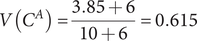
Equation (6)) yields an overall variety score for concept space
$ {C}^A $
 in a scale of
$ 0 $
in a scale of
$ 0 $
 to
$ 1 $
to
$ 1 $
 ,
$ V\left({C}^A\right)=\frac{3.85+6}{10+6}=0.615 $
,
$ V\left({C}^A\right)=\frac{3.85+6}{10+6}=0.615 $
 .
.
Metric proposed by Ahmed
Ahmed et al. (Reference Ahmed, Ramachandran, Fuge, Hunter and Miller2021) described the Sharma–Mittal entropy (SME) as a generalized class of methods for measuring diversity (or variety) in other “non-engineering” domains. They have shown that the Herfindahl index [also known as Herfindahl–Hirschman index (HHI)], adopted by Verhaegen et al. (Reference Verhaegen, Vandevenne, Peeters and Duflou2013), can also be derived from SME. However, instead of using the inverse of the Herfindahl index, they have proposed a variant of the HHI named HHID (i.e., Herfindahl–Hirschman index for design) as a new metric for measuring variety. According to the proposed method, the variety measure of a concept space at an abstraction level
$ \alpha $
 can be written as follows:

Ahmed et al. (Reference Ahmed, Ramachandran, Fuge, Hunter and Miller2021) have compared the above-proposed metric with other existing variety metrics by Shah et al. (Reference Shah, Smith and Vargas-Hernandez2003) and Nelson et al. (Reference Nelson, Wilson, Rosen and Yen2009). They have shown that the HHID has advantages over the existing metrics regarding accuracy, sensitivity, optimizability, and generalizability. Accuracy was measured with respect to ground truth data sets constructed by experts, and it was found that the HHID-based scores align better with human ratings compared to the other two existing measures. Ahmed et al. (Reference Ahmed, Ramachandran, Fuge, Hunter and Miller2021) proposed an empirical method of evaluating metric sensitivity by randomly selecting sets of different concepts and comparing the scores obtained by different metrics. The results showed that Shah’s and Nelson’s metrics gave the same scores to a large percentage of sets and thus proved less sensitive compared to HHID. They have also stated that the HHID closely follows the Gini–Simpson index (GSI), commonly used as a measure of diversity in ecology, given as follows:

In Eq. (8),
$ \lambda $
 is known as the Simpson index (Simpson, Reference Simpson1949).
$ {\pi}_i\left(i=1\dots Z\right) $
is known as the Simpson index (Simpson, Reference Simpson1949).
$ {\pi}_i\left(i=1\dots Z\right) $
 are the proportions of individuals in the various groups in an infinite population where each individual belongs to one of
$ Z $
are the proportions of individuals in the various groups in an infinite population where each individual belongs to one of
$ Z $
 groupings.
$ \lambda $
groupings.
$ \lambda $
 can be interpreted as the probability that two individuals that are randomly and independently picked from the population belong to the same group. In contrast, the complement of
$ \lambda $
can be interpreted as the probability that two individuals that are randomly and independently picked from the population belong to the same group. In contrast, the complement of
$ \lambda $
 in Eq. (8) equals the probability that the two individuals belong to different groups. This is also known as the probability of inter-species encounter (Hurlbert, Reference Hurlbert1971).
It is important to note that the HHID given in Eq. (7) is defined for a sample concept space with
$ N $
 concepts, where the estimate of
$ \lambda $
concepts, where the estimate of
$ \lambda $
 , i.e.,
$ \hat{\lambda} $
, i.e.,
$ \hat{\lambda} $
 , is considered as
$ {\sum}_{i=1}^{\beta_{\alpha }}{\left(\frac{n_i^{\alpha }}{N}\right)}^2 $
, is considered as
$ {\sum}_{i=1}^{\beta_{\alpha }}{\left(\frac{n_i^{\alpha }}{N}\right)}^2 $
 . However, using the unbiased estimate of
$ \lambda $
. However, using the unbiased estimate of
$ \lambda $
 , given by Simpson (Reference Simpson1949), Eq. (7) can be modified as follows:

We may refer to Eq. (8) as the Gini–Simpson index for design (GSID). Equation (8)) is also known as the Gini–Simpson diversity index and is widely used by ecologists as a well-known conventional index for measuring diversity in an ecosystem (Chen et al., Reference Chen, Wu and Shen2018; Augousti et al., Reference Augousti, Atkins, Ben-Naim, Bignall, Hunter, Tunnicliffe and Radosz2021). The unbiased estimate of
$ \lambda $
 used in Eq. (8) is also equivalent to the normalized HHI (Cracau and Duŕan Lima, Reference Cracau and Duŕan Lima2016). Now, applying Eq. (7) to the concept space
$ {C}^A $
used in Eq. (8) is also equivalent to the normalized HHI (Cracau and Duŕan Lima, Reference Cracau and Duŕan Lima2016). Now, applying Eq. (7) to the concept space
$ {C}^A $
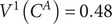
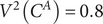
 results in variety scores
$ {V}^1\left({C}^A\right)=0.48 $
results in variety scores
$ {V}^1\left({C}^A\right)=0.48 $
 and
$ {V}^2\left({C}^A\right)=0.8 $
and
$ {V}^2\left({C}^A\right)=0.8 $
 at
$ \alpha =1 $
at
$ \alpha =1 $
 and
$ \alpha =2 $
and
$ \alpha =2 $
 , respectively, whereas Eq. (9) yields variety scores
$ {V}^1\left({C}^A\right)=0.6 $
, respectively, whereas Eq. (9) yields variety scores
$ {V}^1\left({C}^A\right)=0.6 $
 and
$ {V}^2\left({C}^A\right)=1 $
and
$ {V}^2\left({C}^A\right)=1 $
 at
$ \alpha =1 $
at
$ \alpha =1 $
 and
$ \alpha =2 $
and
$ \alpha =2 $
 , respectively. For large sample sizes (
$ N\to \infty $
, respectively. For large sample sizes (
$ N\to \infty $
 ), GSID asymptotically follows the HHID. The advantage of using GSID instead of HHID as a measure for variety in engineering design is further discussed in Section “Research gap: issues with existing variety metrics.”
Research gap: issues with existing variety metrics
To investigate the issues with the aforementioned variety metrics, we consider two essential properties, “accuracy” and “sensitivity,” that make a variety metric reliable. The properties are discussed as follows. Ahmed et al. (Reference Ahmed, Ramachandran, Fuge, Hunter and Miller2021) proposed a procedure for empirically estimating the accuracy of a variety metric by comparing its alignment with a ground truth data set. The ground truth data sets were prepared considering expert feedback, domain knowledge, or consensus from many individuals. Here, the property of “accuracy” implies the validity of a metric. A measure can only be validated against an external frame of reference or a universally accepted standard. Using experts’ ratings to ensure the validity of a metric is a common practice in creativity research (Hennessey et al., Reference Hennessey, Amabile and Mueller1999). HHID, as a metric for measuring design variety [Eq. (7)], was validated by Ahmed et al. (Reference Ahmed, Ramachandran, Fuge, Hunter and Miller2021) against two ground truth data sets; one was established by using pairwise comparisons between sets of polygons, and the other was constructed using milk frother design sketches. Experiments were conducted to benchmark the HHID with the commonly used variety metrics given by Shah et al. (Reference Shah, Smith and Vargas-Hernandez2003) and Nelson et al. (Reference Nelson, Wilson, Rosen and Yen2009). Results from the experiments showed that HHID outperforms the other two metrics in terms of “accuracy.”
However, in this research, we adopted a theoretical approach to evaluate existing metrics in terms of “accuracy.” We use the mathematical definition of variety employed by Ahmed et al. (Reference Ahmed, Ramachandran, Fuge, Hunter and Miller2021) to formulate the property of “accuracy,” as given below.
Property 1
(Accuracy). Considering a particular abstraction level
$ \alpha $
 , the variety score provided by a metric should tell us the probability that two concepts selected at random (without replacement) from a sample concept space will belong to different idea groups (i.e., different nodes of a genealogy tree) at abstraction level
$ \alpha $
, the variety score provided by a metric should tell us the probability that two concepts selected at random (without replacement) from a sample concept space will belong to different idea groups (i.e., different nodes of a genealogy tree) at abstraction level
$ \alpha $
 .
.
Apart from “accuracy,” a metric can also be evaluated in terms of “sensitivity.” The property of “sensitivity” is defined as follows.
Property 2
(Sensitivity). In an ideal case, a variety metric should be able to reflect a change in measurement with varying numbers of concepts in a concept space, i.e.,
$ N $
 , as well as the distribution of concepts over the
$ {\beta}_{\alpha } $
, as well as the distribution of concepts over the
$ {\beta}_{\alpha } $
 nodes in the idea space
$ {I}^{\alpha } $
nodes in the idea space
$ {I}^{\alpha } $
 , denoted by
$ {n}_i^{\alpha } $
, denoted by
$ {n}_i^{\alpha } $
 .
.
For example, let us consider another example of concept space,
$ {C}^B $
 , illustrated in Figure 3, where a designer explores ideas to fulfil the function of “pumping water.” The ideas at the physical principle level are identical to
$ {C}^A $
, illustrated in Figure 3, where a designer explores ideas to fulfil the function of “pumping water.” The ideas at the physical principle level are identical to
$ {C}^A $
 (see Fig. 1): “centrifugal force” and “positive displacement.” Five concepts are generated based on these two physical principles, each representing a distinct idea at the working principle level. The genealogy tree of the concept space,
$ {C}^B $
(see Fig. 1): “centrifugal force” and “positive displacement.” Five concepts are generated based on these two physical principles, each representing a distinct idea at the working principle level. The genealogy tree of the concept space,
$ {C}^B $
 , is shown in Figure 4. Unlike
$ {C}^A $
, is shown in Figure 4. Unlike
$ {C}^A $
 , in the case of
$ {C}^B $
, in the case of
$ {C}^B $
 , 4 out of 5 concepts share identical ideas (“positive displacement”) at the physical principle level (as shown in Fig. 3). This results in different
$ {n}_i^{\alpha } $
, 4 out of 5 concepts share identical ideas (“positive displacement”) at the physical principle level (as shown in Fig. 3). This results in different
$ {n}_i^{\alpha } $
 values for
$ {C}^A $
values for
$ {C}^A $
 and
$ {C}^B $
and
$ {C}^B $
 at the physical principle level, and a “good” variety metric should reflect this difference while accurately providing the variety scores for these two concept spaces. In ecology, this property implies the “evenness sensitivity” of a diversity (or variety) measure (Crupi, Reference Crupi, Casetta, da Silva and Vecchi2019).
Concept space (
$ {C}^B $
 ) generated by combining different ideas from different levels of abstraction.

Figure 3. Long description
The flowchart is divided into three horizontal layers separated by dashed lines.
At the top level, labeled Function on the right, a yellow box contains the text To pump water.
Two curved arrows lead down to the second level, labeled Physical principle alpha = 1. This level contains two red boxes. The left box is labeled I sub 1 super 1 Centrifugal Force. The right box is labeled I sub 2 super 1 Positive Displacement.
The third level is labeled Working principle alpha = 2 and contains five green boxes.
An arrow from Centrifugal Force points to a single green box on the left labeled I sub 1 super 2, which describes utilizing a rotating impeller to impart kinetic energy to water, converted to pressure energy in a volute casing.
Four arrows from Positive Displacement point to a vertical stack of green boxes on the right.
- I sub 2 super 2 describes using a piston inside a cylinder with a crankshaft.
- I sub 3 super 2 describes employing a flexible diaphragm to create pressure changes.
- I sub 4 super 2 describes utilizing rotating vanes or blades inside a housing.
- I sub 5 super 2 describes employing intermeshing gears inside a casing to carry water from inlet to outlet.
Tree constructed from concept space
$ {C}^B $
 .
.

In the following sections, we follow a theoretical approach to evaluate the accuracy and sensitivity of the existing metrics. We argue that GSID [Eq. (9)] can be used as a refined version of HHID [Eq. (7)] to provide better accuracy and sensitivity for genealogy tree-based variety assessment compared to other existing metrics. The argument is supported by at least two test cases where the existing metrics are not found to be accurate or sensitive. The variety metrics proposed by Shah, Nelson, Verhaegen, and Ahmed are hereafter referred to as “SVS,” “NM,” “IHI,” and “HHID,” respectively.
Test Case I
Consider a concept space with
$ N $
 number of concepts. At an abstraction level
$ \alpha $
number of concepts. At an abstraction level
$ \alpha $
 (e.g., “physical principle” in Fig. 1), the total number of ideas or nodes is two, i.e.,
$ {\beta}_{\alpha }=2 $
(e.g., “physical principle” in Fig. 1), the total number of ideas or nodes is two, i.e.,
$ {\beta}_{\alpha }=2 $
 (e.g., “centrifugal force” and “positive displacement”). Now, there could exist different concept spaces with an identical number of total concepts, say
$ N=20 $
(e.g., “centrifugal force” and “positive displacement”). Now, there could exist different concept spaces with an identical number of total concepts, say
$ N=20 $
 , but with different distributions of concepts over the two nodes, as shown in Figure 5. In this case, adhering to the definition of accuracy and sensitivity, a compelling variety metric should satisfy the following three conditions: (a) It should give the maximum score to a completely even distribution of concepts over the two nodes in the idea space (i.e.,
$ {n}_1^{\alpha }={n}_2^{\alpha }=\frac{N}{2} $
, but with different distributions of concepts over the two nodes, as shown in Figure 5. In this case, adhering to the definition of accuracy and sensitivity, a compelling variety metric should satisfy the following three conditions: (a) It should give the maximum score to a completely even distribution of concepts over the two nodes in the idea space (i.e.,
$ {n}_1^{\alpha }={n}_2^{\alpha }=\frac{N}{2} $
 ) as the probability that two concepts that are randomly and independently selected from the concept space share different ideas from the idea space
$ {I}^{\alpha } $
) as the probability that two concepts that are randomly and independently selected from the concept space share different ideas from the idea space
$ {I}^{\alpha } $
 is maximum in this case; (b) a lower variety score should be given for a skewed distribution of concepts over the two nodes in the idea space; and (c) the score at
$ \alpha $
is maximum in this case; (b) a lower variety score should be given for a skewed distribution of concepts over the two nodes in the idea space; and (c) the score at
$ \alpha $
 should be strictly
$ 0 $
should be strictly
$ 0 $
 when all the concepts share identical ideas (e.g., all the concepts share a similar physical principle – “centrifugal force”).
Example concept spaces for Test Case I with different distributions of concepts over the two nodes at an abstraction level α.

Figure 6 presents the scores, scaled to a range of 0 to 1 (with 1 indicating the maximum variety), provided by different variety metrics for different distributions of 20 concepts over two nodes at α. For example,
$ ``5/15 $
 ” on the x-axis denotes the distribution of 20 pump concepts at the physical principle level, where five concepts work based on “centrifugal force,” and the remaining
$ 15 $
” on the x-axis denotes the distribution of 20 pump concepts at the physical principle level, where five concepts work based on “centrifugal force,” and the remaining
$ 15 $
 concepts work based on “positive displacement.” As shown in Figure 6, the SVS and NM scores remain constant for both even and skewed distributions except for the
$ ``0/20 $
concepts work based on “positive displacement.” As shown in Figure 6, the SVS and NM scores remain constant for both even and skewed distributions except for the
$ ``0/20 $
 ” distribution, where the score changes from a constant value to
$ 0 $
” distribution, where the score changes from a constant value to
$ 0 $
 , and this is due to the change in
$ {\beta}_{\alpha } $
, and this is due to the change in
$ {\beta}_{\alpha } $
 value from
$ 2 $
value from
$ 2 $
 to
$ 1 $
to
$ 1 $
 . From this observation, it can be concluded that both SVS and NM lack “sensitivity,” leading to inaccurate variety scores for this test case. In the case of IHI, HHID, and GSID, the scores gradually decrease when the distribution of concepts becomes more skewed and, thus, these three metrics satisfy the property of “sensitivity.” However, for the
$ "0/20 $
. From this observation, it can be concluded that both SVS and NM lack “sensitivity,” leading to inaccurate variety scores for this test case. In the case of IHI, HHID, and GSID, the scores gradually decrease when the distribution of concepts becomes more skewed and, thus, these three metrics satisfy the property of “sensitivity.” However, for the
$ "0/20 $
 ” distribution, unlike the other metrics, IHI gives a score of
$ 0.05 $
” distribution, unlike the other metrics, IHI gives a score of
$ 0.05 $
 instead of
$ 0 $
instead of
$ 0 $
 . Hence, IHI provides an inaccurate score (violating Property 1) for any finite value of
$ N $
. Hence, IHI provides an inaccurate score (violating Property 1) for any finite value of
$ N $
 when
$ {\beta}_{\alpha }=1 $
when
$ {\beta}_{\alpha }=1 $
 . Overall, for Test Case I, both HHID and GSID are found to be more compelling compared to the others in terms of both “accuracy” and “sensitivity.”
Illustration of the Test Case I.

Figure 6. Long description
The line graph features a vertical Y-axis labeled Variety score at abstraction level alpha, ranging from 0.00 to 0.60 in increments of 0.05. The horizontal X-axis is labeled Distribution of the concepts over the nodes at abstraction level alpha, with eleven categorical points: 10/10, 9/11, 8/12, 7/13, 6/14, 5/15, 4/16, 3/17, 2/18, 1/19, and 0/20.
Five data series are plotted:
* G S I D (red triangles): Starts at the highest variety score of approximately 0.53 and follows a downward concave curve, dropping sharply after 4/16 to reach 0.00 at 0/20.
* H H I D (green squares): Follows a nearly identical downward concave path as G S I D, starting slightly lower at 0.50 and converging with G S I D at 1/19 (score 0.10) and 0/20 (score 0.00).
* S V S (black crosses): Maintains a perfectly horizontal linear trend at a variety score of 0.10 from 10/10 until 1/19, then drops to 0.00 at 0/20.
* I H I (orange diamonds): Shows a gradual linear decrease from 0.10 at 10/10 down to 0.05 at 0/20.
* N M (blue circles): Maintains a constant horizontal line at a variety score of approximately 0.05 from 10/10 until 1/19, then drops to 0.00 at 0/20.
Test Case II
In this test case, we consider different concept spaces, as shown in Figure 7, where for each concept space, the concepts are evenly distributed over two nodes in an idea space
$ {I}^{\alpha } $
 . For example, if there are
$ N $
. For example, if there are
$ N $
 pump concepts,
$ N/2 $
pump concepts,
$ N/2 $
 of them work based on “centrifugal force,” and the rest
$ N/2 $
of them work based on “centrifugal force,” and the rest
$ N/2 $
 work based on “positive displacement,” i.e.,
$ {n}_1^{\alpha }={n}_2^{\alpha }=N/2 $
work based on “positive displacement,” i.e.,
$ {n}_1^{\alpha }={n}_2^{\alpha }=N/2 $
 . Now, consider there are only two concepts in the concept space, i.e.,
$ N=2, $
. Now, consider there are only two concepts in the concept space, i.e.,
$ N=2, $
 and both of them have distinct physical principles. In this case, for the abstraction level “physical principle,” adhering to the definition of accuracy (Property 1), the variety score is expected to be
$ 1 $
and both of them have distinct physical principles. In this case, for the abstraction level “physical principle,” adhering to the definition of accuracy (Property 1), the variety score is expected to be
$ 1 $
 (considering the variety metric provides a score in the range
$ 0 $
(considering the variety metric provides a score in the range
$ 0 $
 to
$ 1 $
to
$ 1 $
 , and
$ 1 $
, and
$ 1 $
 denoting the maximum variety). If
$ N $
denoting the maximum variety). If
$ N $
 is large, considering the definition of accuracy (Property 1), the variety score should asymptotically follow the value
$ 0.5 $
is large, considering the definition of accuracy (Property 1), the variety score should asymptotically follow the value
$ 0.5 $
 , which is the probability that two concepts randomly and independently selected from the concept space (with
$ N\to \infty $
, which is the probability that two concepts randomly and independently selected from the concept space (with
$ N\to \infty $
 ) are different at the physical principle level.
Example concept spaces for Test Case II with similar distributions of concepts over the two nodes at an abstraction level α.

Figure 7. Long description
The diagram consists of five square panels arranged horizontally, with an ellipsis between the third and fourth panels.
* Each panel contains a three-node tree structure. The top node represents the Total number of concepts N, and the two bottom nodes represent the Abstraction level alpha.
* Panel C sub 1: Top node contains 2. Bottom nodes both contain 1.
* Panel C sub 2: Top node contains 4. Bottom nodes both contain 2.
* Panel C sub 3: Top node contains 6. Bottom nodes both contain 3.
* Panel C sub 19: Top node contains 38. Bottom nodes both contain 19.
* Panel C sub 20: Top node contains 40. Bottom nodes both contain 20.
Below the panels, the Expected Variety Score is indicated. Under C sub 1, the score is V super alpha equals 1. Under C sub 20, the score is V super alpha is approximately 0.5. An ellipsis indicates the progression of values between the two extremes.
Considering the case described above, the scores given by different variety metrics, scaled to a range of
$ 0 $
 to
$ 1 $
to
$ 1 $
 , are plotted in Figure 8, where
$ N $
, are plotted in Figure 8, where
$ N $
 ranges from
$ 2\;\mathrm{to}\;40 $
ranges from
$ 2\;\mathrm{to}\;40 $
 (note that the range is chosen arbitrarily). It can be observed that, unlike other metrics, the scores calculated using HHID remain unchanged for varying
$ N $
(note that the range is chosen arbitrarily). It can be observed that, unlike other metrics, the scores calculated using HHID remain unchanged for varying
$ N $
 . HHID also provides an “inaccurate” score for
$ N=2 $
. HHID also provides an “inaccurate” score for
$ N=2 $
 , i.e.,
$ 0.5 $
, i.e.,
$ 0.5 $
 instead of
$ 1 $
instead of
$ 1 $
 . It can be noticed that the score, that HHID gives for any finite value of
$ N $
. It can be noticed that the score, that HHID gives for any finite value of
$ N $
 , is nothing but the score obtained from GSID for
$ N\to \infty $
, is nothing but the score obtained from GSID for
$ N\to \infty $
 . This has occurred because of using a “biased” estimator of the Simpson index
$ \left[\unicode{x03BB}, \mathrm{see}\;\mathrm{Eq}.(8)\right] $
. This has occurred because of using a “biased” estimator of the Simpson index
$ \left[\unicode{x03BB}, \mathrm{see}\;\mathrm{Eq}.(8)\right] $
 while defining HHID [see Eq. (7)]. The bias is significant when
$ N $
while defining HHID [see Eq. (7)]. The bias is significant when
$ N $
 is small and thus leads to an “inaccurate” measure of variety, violating Property 1. The other three metrics, i.e., SVS, NM, and IHI, are found to be “accurate” for
$ N=2 $
is small and thus leads to an “inaccurate” measure of variety, violating Property 1. The other three metrics, i.e., SVS, NM, and IHI, are found to be “accurate” for
$ N=2 $
 . However, when
$ N $
. However, when
$ N $
 is large, these three metrics provide variety scores, which asymptotically diminish to the value
$ 0 $
is large, these three metrics provide variety scores, which asymptotically diminish to the value
$ 0 $
 instead of following the value
$ 0.5 $
instead of following the value
$ 0.5 $
 and hence are found to be “inaccurate,” or violating Property 1. Theoretically, one can also observe from Eq. (2) and Eq. (3) that the cases when
$ {\beta}_{\alpha } $
and hence are found to be “inaccurate,” or violating Property 1. Theoretically, one can also observe from Eq. (2) and Eq. (3) that the cases when
$ {\beta}_{\alpha } $
 is much smaller compared to
$ N $
is much smaller compared to
$ N $
 , both SVS and NM will give a score close to
$ 0 $
, both SVS and NM will give a score close to
$ 0 $
 irrespective of the distribution of
$ N $
irrespective of the distribution of
$ N $
 concepts over the
$ {\beta}_{\alpha } $
concepts over the
$ {\beta}_{\alpha } $
 nodes in the idea space. The same is true for IHI as well. For a smaller
$ {\beta}_{\alpha } $
nodes in the idea space. The same is true for IHI as well. For a smaller
$ {\beta}_{\alpha } $
 and larger
$ N $
and larger
$ N $
 , in Eq. (5), the denominator value becomes much greater than the numerator because of the large square terms in the denominator, which ultimately reduces the variety score close to
$ 0 $
, in Eq. (5), the denominator value becomes much greater than the numerator because of the large square terms in the denominator, which ultimately reduces the variety score close to
$ 0 $
 .
.
Illustration of the Test Case II.

Figure 8. Long description
The Y-axis is labeled Variety score at abstraction level alpha, ranging from 0.0 to 1.0. The X-axis is labeled Distribution of the concepts over the nodes at abstraction level alpha, with fractional values from 1/1 to 20/20.
Five data series are plotted:
1. G S I D (red triangles): Starts at 1.0, drops sharply to 0.67 at 2/2, and then follows an asymptotic curve that levels off at approximately 0.5.
2. H H I D (green squares): Maintains a perfectly horizontal linear trend at a constant variety score of 0.5 across all X-axis values.
3. S V M (black X marks): Overlays exactly with I H I and N M at specific points. It starts at 1.0, drops to 0.5 at 2/2, 0.33 at 3/3, and continues a steep decay toward 0.05.
4. I H I (orange diamonds): Follows the same steep decay path as S V M, starting at 1.0 and curving down to approximately 0.05 at the 20/20 mark.
5. N M (blue circles): Shows the steepest initial decline, dropping from 1.0 to approximately 0.33 at 2/2 and 0.2 at 3/3, eventually converging with S V M and I H I near the 0.03 mark at the far right of the graph.
Rationale for introducing a new distance-based variety metric
Test Cases I and II suggest that for genealogy tree-based variety assessment, the “bias-corrected” GSID is a better metric for assessing the variety of a concept space compared to other existing metrics. Additionally, Test Case II implies that in the future, researchers should consider an “unbiased” estimator of any existing entropy-based measure, such as the SME (Ahmed et al., Reference Ahmed, Ramachandran, Fuge, Hunter and Miller2021), while proposing a new metric.
However, a major assumption for all the existing tree-based variety assessment approaches is that all the ideas in the idea space are considered equally distant. Let us consider an example where three different types of clutches are there in a concept space: plate clutch (
$ {C}_1 $
 ), centrifugal clutch (
$ {C}_2 $
), centrifugal clutch (
$ {C}_2 $
 ), and electromagnetic clutch (
$ {C}_3 $
), and electromagnetic clutch (
$ {C}_3 $
 ). If we consider the idea space for “driving input” (representing a design attribute or an abstraction level), then the three different ideas with respect to
$ {C}_1 $
). If we consider the idea space for “driving input” (representing a design attribute or an abstraction level), then the three different ideas with respect to
$ {C}_1 $
 ,
$ {C}_2 $
,
$ {C}_2 $
 , and
$ {C}_3 $
, and
$ {C}_3 $
 are “spring force,” “centrifugal force,” and “electric current,” respectively. In this case, a domain expert may find “spring force” and “centrifugal force” to be more similar to each other compared to “electric current.” Thus, constructing a tree-like structure or grouping ideas in distinct nodes becomes difficult when the distance variable between two ideas is continuous instead of binary. In such cases, none of the existing metrics are applicable as a measure of variety. The same limitation of existing metrics was also pointed out by Ahmed et al. (Reference Ahmed, Ramachandran, Fuge, Hunter and Miller2021).
From Eqs. (2), (3), and (5), it can be observed that SVS, NM, and IHI metrics use the weight of each function (that a design concept needs to satisfy) to assess variety. However, these function weights relate to the value or usefulness of a concept, rather than its variety. Variety should indicate how different one concept is from others, not how good or important the delivered functions are relative to one another. Consequently, using function weights conflates the assessment of concept variety with evaluations of concept quality.
The existing variety metrics discussed in this article have used four abstraction or hierarchical levels (physical principle, working principle, embodiment, and detail) to represent a concept. These four levels were first introduced by Shah et al. (Reference Shah, Smith and Vargas-Hernandez2003). However, the distinction between a physical principle and a working principle remains unclear, and there is a lack of comprehensive guidelines to break a design concept into these four abstraction levels. For instance, Ramachandran et al. (Reference Ramachandran, Fuge, Hunter and Miller2018) reported their struggle to define the physical and working principles appropriately while creating genealogy trees for the design concepts. Hence, it is up to the designers to carefully describe the principles of the design concepts to ensure repeatability of their variety scores. The problem becomes more evident for complex design concepts, which may use multiple physical principles at different operating states to satisfy an intended function (Majumder et al., Reference Majumder, Bhatt, Chakrabarti, Chakrabarti and Singh2023). For example, a hair dryer can have two operating states:
$ O{N}_1 $
 and
$ O{N}_2 $
and
$ O{N}_2 $
 . At
$ O{N}_1 $
. At
$ O{N}_1 $
 , it uses two physical principles, “heating” and “blowing” of air, whereas, at
$ O{N}_2 $
, it uses two physical principles, “heating” and “blowing” of air, whereas, at
$ O{N}_2 $
 , it only uses “blowing” of air to satisfy the intended function. Hence, it is important to choose an appropriate knowledge representation scheme, which can describe a complex design concept more comprehensively.
Our work addresses the above issues from three different aspects:
-
1. Eliminating the requirement of genealogy tree-based representation: We eliminate the requirement of genealogy tree-based representation of the concept space and provide a new distance-based variety metric, based on Rao’s quadratic diversity index (Rao, Reference Rao1982), that is applicable to measure the variety of a concept space irrespective of which abstraction levels and how many of them are considered while representing the concepts.
-
2. Providing a flexible framework for representing and comparing concepts: In addition to introducing the new metric, we offer a framework for assessing variety that allows design concepts to be described using any preferred representation scheme and level of abstraction. Within this framework, the distance between two concepts at an abstraction level $ \alpha $
 is measured by analyzing the semantic similarity between their respective descriptions, and all pairwise distances are stored in a distance matrix. This flexibility enables designers to work with representations that best suit their domain or design problem context.
 -
3. Developing a tool to support the variety assessment process: A software tool – “VariAnT” (Variety Assessment Tool) – has also been developed to automate the variety assessment process for a given design concept space.

A prescriptive framework for assessing variety
The overall procedural breakdown of the prescriptive variety assessment framework is depicted in Figure 9. In the following part of this section, we elaborate on the framework. First, we present a knowledge representation scheme for storing the design concepts into a structured data frame. Next, we demonstrate a method for measuring the distance between two design concepts by comparing the textual descriptions across different abstraction levels, utilizing a state-of-the-art natural language processing (NLP) technique. Following this, we propose a new variety metric based on an unbiased estimate of Rao’s quadratic diversity index (Rao, Reference Rao1982) and introduce the “VariAnT” tool, which embodies the proposed framework. Finally, we provide an example to demonstrate the variety calculation using the new framework.
The overall procedural breakdown of the proposed variety assessment framework.

Figure 9. Long description
The flowchart consists of six main stages connected by arrows.
1. Concept Space: A box containing Concept 1, Concept 2, an ellipsis, and Concept N.
2. DataFrame: An arrow points from Concept Space to a grid representing a data table with rows and columns.
3. Embeddings: An arrow points from DataFrame to a box containing three colored horizontal vector representations (purple, green, and blue) with ellipses.
4. Pairwise Distance: An arrow points to a dashed box showing two vectors (orange and teal) with a double-headed arrow between them.
5. Distance Matrices: An arrow points to a stacked series of 8 by 8 grids. An arrow labeled Abstraction Levels points diagonally upward. The matrices show a diagonal of zeros.
6. Proposed Variety Metric: A line from the bottom of the Distance Matrices points to a green-header box labeled R Q I D (Rao's Quadratic Index for Design).
7. Variety Scores: A final arrow points from the R Q I D box to an oval labeled Variety Scores.
Knowledge representation
Different representation schemes and complexities
Design concepts can be represented at different levels of abstraction, and several modelling schemes in the literature support such multi-level descriptions. For example, the Function–Behavior–Structure (FBS) model (Gero and Kannengiesser, Reference Gero and Kannengiesser2004) represents concepts through the relationships between what a system is intended to do (function), how it does it (behavior), and what it is composed of (structure). Similarly, Chakrabarti et al. (Reference Chakrabarti, Sarkar, Leelavathamma and Nataraju2005) introduced SAPPhIRE, a causality model that describes systems across a richer set of abstraction levels, namely, States, Actions, Parts, Phenomena, Inputs, oRgans, and Effects. The interrelationships among these constructs, as depicted in Figure 10a, can be summarized as follows: Parts, which encompass physical components and interfaces, play a crucial role in the formation of oRgans, which represent the properties and conditions of a system and its environment necessary for the interaction. oRgans, in conjunction with Input(s) in the form of material, energy, or information, collectively trigger physical Effect(s), which subsequently give rise to physical Phenomena and induce a State change in the system. This State change is further interpreted as Action(s), an abstract description of an interaction that can serve as an input or create/activate (new) Part(s). Figure 10b shows an example where the SAPPhIRE model explains how a hot body cools down in the presence of a surrounding fluid medium.
(a) The SAPPhIRE model of causality (Chakrabarti et al., Reference Chakrabarti, Sarkar, Leelavathamma and Nataraju2005). (b) An example SAPPhIRE model explaining how a hot body cools down (Srinivasan and Chakrabarti, Reference Srinivasan and Chakrabarti2009).

Figure 10. Long description
Panel a shows the theoretical S A P P h I R E model. At the base is Parts, which Create o R gans. Above this, Inputs and o R gans together Activate Effects. Effects Create Phenomena, which in turn Create State changes. At the top, State changes are Interpreted as Actions. Feedback loops show Actions connecting back to Parts via a Create path, and State changes connecting back to Inputs via an Interpreted as path.
Panel b applies this model to a cooling body.
- Parts: A body held in a fluid medium.
- o R gans: Constant surface area of the body and the heat transfer coefficient between the body and the surrounding fluid medium.
- Inputs: Temperature difference between the body and the surroundings.
- Effects: Newton's law of cooling.
- Phenomena: Transfer of heat from the body to the surrounding fluid medium.
- State changes: A decrease in the heat energy in the body.
- Actions: Rapid cooling of the body.
Representation of the concept space in a data frame.

Figure 11. Long description
The diagram is structured as a complex table. The vertical axis on the left is labeled Concept I D, containing rows for 1, a vertical ellipsis, and N. Adjacent to this is the Instance I D column, which further divides each Concept I D into sub-rows labeled k, starting with 1, followed by a vertical ellipsis, and ending with k sub 1 for Concept 1, or k sub N for Concept N. The horizontal axis at the top is labeled Abstraction levels (e sub N super alpha k) with an arrow pointing right. The header row for these levels lists alpha equals 1, alpha equals 2, alpha equals 3, alpha equals 4, alpha equals 5, an ellipsis, and alpha equals m. The internal cells contain mathematical elements e. For Concept 1, Instance 1, the cells are e sub 1 super 11 through e sub 1 super m1. For Concept 1, Instance k sub 1, the cells are e sub 1 super 1k sub 1 through e sub 1 super mk sub 1. This pattern repeats for Concept N, where Instance 1 contains cells e sub N super 11 through e sub N super m1, and Instance k sub N contains cells e sub N super 1k sub N through e sub N super mk sub N. Horizontal ellipses indicate omitted rows between Concept 1 and Concept N.
In comparison to the FBS model, in SAPPhIRE, the “action” encompasses the notion of “function,” while “parts” can be understood as “structure.” The remaining constructs of SAPPhIRE collectively contribute to a comprehensive depiction of “behavior.” Many systems can be represented using a single instance of a SAPPhIRE model. However, when dealing with complex systems that necessitate more detailed descriptions, multiple SAPPhIRE models are required for representation. By using multiple instances of the SAPPhIRE, Siddharth et al. (Reference Siddharth, Chakrabarti and Venkataraman2018) created causal chains to represent the functioning of a complex system, which provides elements of description that are absent in other existing models. In our past work (Majumder et al., Reference Majumder, Bhatt, Chakrabarti, Chakrabarti and Singh2023), we found that the majority of existing models lack an explanation of how to model the functionalities of a system with multiple operating states (also referred to as multi-state systems), and the models that do consider multiple operating states do not explicitly explain a method to capture the underlying causal relationships inherent within the system. To address these issues, we proposed an integrated function modelling approach using SAPPhIRE as the basis (Majumder et al., Reference Majumder, Bhatt, Chakrabarti, Chakrabarti and Singh2023). Broadly, the proposed approach uses the model of a “transformation system” (Hubka and Eder, Reference Hubka and Eder1988) to identify the “technical process,” the “operand(s)” (the entity undergoing transformation), and the “technical system” (or the “operator”) responsible for driving the “technical process.” Then, the causal processes associated with the “transformation system” are explained with multiple instances of the SAPPhIRE model. In the past, researchers also reported the use of SAPPhIRE abstraction levels in synthesizing design concepts (Srinivasan and Chakrabarti, Reference Srinivasan and Chakrabarti2009; Bhatt et al., Reference Bhatt, Majumder and Chakrabarti2021; Trollman et al., Reference Trollman, Jagtap and Trollman2023). For example, Trollman et al. (Reference Trollman, Jagtap and Trollman2023) employed the SAPPhIRE model to conceptualize different strategies for countering speculative wheat market fluctuations. Additionally, multiple software tools, such as IDEA-INSPIRE (Chakrabarti et al., Reference Chakrabarti, Siddharth, Dinakar, Panda, Palegar and Keshwani2017) and OPAL (Peters et al., Reference Peters, Fortin and McSorley2021), were developed by researchers that utilize the SAPPhIRE model to create a database of existing design concepts that can be further utilized as design stimuli acting as a design-by-analogy tool. The SAPPhIRE model has also been used to capture the knowledge obtained during the testing phases of product design, such as the potential failure modes (Siddharth et al., Reference Siddharth, Chakrabarti and Ranganath2020).
The above discussion motivates the need for a representation approach that supports multiple descriptive instances, regardless of the specific modeling framework used. Each instance corresponds to a chosen abstraction level or modeling construct (e.g., function, behavior, structure, input), and a concept may require one or many such instances depending on its complexity. The framework introduced in this article operates on these instances without imposing any specific modelling scheme, allowing designers to choose the representation that best suits their domain or design problem.
Concept space data frame
Assuming that we already have explored a concept space
$ C $
 – comprised of
$ N $
– comprised of
$ N $
 concepts – for a given design problem, each concept in the concept space can be represented with a single instance or a set of instances. For the
$ {i}^{th} $
concepts – for a given design problem, each concept in the concept space can be represented with a single instance or a set of instances. For the
$ {i}^{th} $
 concept (
$ {C}_i $
concept (
$ {C}_i $
 ), the associated set of instances can be represented as follows:

where
$ \alpha $
 takes values ranging from
$ 1 $
takes values ranging from
$ 1 $
 –
$ m $
–
$ m $
 , corresponding to different levels of abstraction. For example, if we consider a SAPPhIRE model,
$ \alpha $
, corresponding to different levels of abstraction. For example, if we consider a SAPPhIRE model,
$ \alpha $
 takes values ranging from
$ 1 $
takes values ranging from
$ 1 $
 –
$ 7 $
–
$ 7 $
 , as shown in Figure 11. Here, the concept
$ {C}_i $
, as shown in Figure 11. Here, the concept
$ {C}_i $
 consists of
$ {k}_i $
consists of
$ {k}_i $
 instances of SAPPhIRE, therefore, a list of data or ideas (
$ {S}_i^{\alpha } $
instances of SAPPhIRE, therefore, a list of data or ideas (
$ {S}_i^{\alpha } $
 ) at an abstraction level
$ \alpha $
) at an abstraction level
$ \alpha $
 can be shown as in Eq. (11), where
$ {e}_i^{\unicode{x03B1} k} $
can be shown as in Eq. (11), where
$ {e}_i^{\unicode{x03B1} k} $
 denotes a construct of the
$ {k}^{th} $
denotes a construct of the
$ {k}^{th} $
 instance of the representation model at abstraction level
$ \alpha $
instance of the representation model at abstraction level
$ \alpha $
 .
.

Vector encoding
In this step, the text data stored in the data frame is converted into numerical vectors that can be used to calculate the semantic similarity between the textual data of two concepts at a particular level of abstraction. For each concept, first, we convert the list of strings,
$ {S}_i^{\alpha } $
 , into a single string,
$ {L}_i^{\alpha } $
, into a single string,
$ {L}_i^{\alpha } $
 using a concatenation operation, denoted by
$ ``\oplus $
using a concatenation operation, denoted by
$ ``\oplus $
 ” in Eq. (12):

Next, we consider two such strings:
$ {L}_i^{\alpha } $
 and
$ {L}_j^{\alpha } $
and
$ {L}_j^{\alpha } $
 that are generated from the dataset of the
$ {i}^{th} $
that are generated from the dataset of the
$ {i}^{th} $
 concept and
$ {j}^{th} $
concept and
$ {j}^{th} $
 concept at abstraction level
$ \alpha $
concept at abstraction level
$ \alpha $
 . Then, the strings
$ {L}_i^{\alpha } $
. Then, the strings
$ {L}_i^{\alpha } $
 and
$ {L}_j^{\alpha } $
and
$ {L}_j^{\alpha } $
 are encoded as vectors denoted by
$ \overrightarrow{A_i^{\alpha }} $
are encoded as vectors denoted by
$ \overrightarrow{A_i^{\alpha }} $
 and
$ \overrightarrow{A_j^{\alpha }} $
and
$ \overrightarrow{A_j^{\alpha }} $
 , respectively.
We employ a Sentence-BERT or S-BERT (Reimers and Gurevych, Reference Reimers and Gurevych2019) to generate the text embeddings in our proposed framework. In the recent past, S-BERT was widely used across different design applications for embedding natural language texts and evaluating the semantic similarity. For example, Singh and Chakrabarti (Reference Singh and Chakrabarti2025) used these embeddings to assess the creative potential of design problems, and Wilson and Yang (Reference Wilson and Yang2025) have utilized similar embeddings to evaluate semantic closeness between human and AI-generated design reasoning. In our current version of the proposed variety assessment tool, we use an open-source, state-of-the-art, and lightweight pre-trained sentence transformer model, “all-MiniLM-L6-v2,” provided by HuggingFace (https://huggingface.co/sentence-transformers/all-MiniLM-L6-v2). This model maps the text to a 384-dimensional dense vector space and is widely used for NLP tasks like clustering, semantic search, semantic similarity, and so forth We may also employ other embedding models, such as OpenAI embeddings (https://platform.openai.com/docs/guides/embeddings/embedding-models), universal-sentence-encoder (https://pypi.org/project/spacy-universal-sentence-encoder/), providing access to high-quality, pre-trained language models for various NLP tasks.
Distance matrix
The distance matrix is a
$ N\times N $
 matrix representing all the pairwise distances (or dissimilarity values) between the design concepts. Once we get the vector embeddings for the
$ {i}^{th} $
matrix representing all the pairwise distances (or dissimilarity values) between the design concepts. Once we get the vector embeddings for the
$ {i}^{th} $
 and
$ {j}^{th} $
and
$ {j}^{th} $
 concept at an abstraction level
$ \alpha $
concept at an abstraction level
$ \alpha $
 , the distance
$ {d}_{ij}^{\alpha } $
, the distance
$ {d}_{ij}^{\alpha } $
 between
$ \overrightarrow{A_i^{\alpha }} $
between
$ \overrightarrow{A_i^{\alpha }} $
 and
$ \overrightarrow{A_j^{\alpha }} $
and
$ \overrightarrow{A_j^{\alpha }} $
 is calculated as

where
$ sim\left(\overrightarrow{A_i^{\alpha }},\overrightarrow{A_j^{\alpha }}\right) $
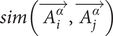 measures the cosine similarity by comparing the orientation of two vectors in a high-dimensional abstract space (Nandy et al., Reference Nandy, Dong and Goucher-Lambert2022). Further, the distance value
$ {d}_{ij}^{\alpha } $
measures the cosine similarity by comparing the orientation of two vectors in a high-dimensional abstract space (Nandy et al., Reference Nandy, Dong and Goucher-Lambert2022). Further, the distance value
$ {d}_{ij}^{\alpha } $
 is calculated by subtracting the cosine similarity value from 1. The distance between any two concepts is associative, i.e.,
$ {d}_{ij}^{\alpha }={d}_{ji}^{\alpha } $
is calculated by subtracting the cosine similarity value from 1. The distance between any two concepts is associative, i.e.,
$ {d}_{ij}^{\alpha }={d}_{ji}^{\alpha } $
 , and for
$ i=j $
, and for
$ i=j $
 ,
$ {d}_{ij}^{\alpha }=0 $
,
$ {d}_{ij}^{\alpha }=0 $
 .
.
Obtaining variety scores
The variety score of the
$ {i}^{th} $
 concept (
$ {C}_i $
concept (
$ {C}_i $
 ) at an abstraction level
$ \alpha $
) at an abstraction level
$ \alpha $
 becomes the average distance of the
$ {i}^{th} $
becomes the average distance of the
$ {i}^{th} $
 concept from the other
$ \left(N-1\right) $
concept from the other
$ \left(N-1\right) $
 concepts in that concept space (
$ C $
concepts in that concept space (
$ C $
 ). Therefore,

The variety score of a concept space (
$ C $
 ) at an abstraction level α becomes the average variety score of all concepts (i.e.,
$ {V}_i^{\alpha } $
) at an abstraction level α becomes the average variety score of all concepts (i.e.,
$ {V}_i^{\alpha } $
 ) in that concept space, as shown in Eq. (15):

The expression of
$ {V}^{\alpha } $
 in Eq. (15), derived using simple heuristics, is equivalent to an unbiased estimator of Rao’s quadratic diversity index (Rao, Reference Rao1982) – one of the widely used measures of ecological diversity (Pavoine et al., Reference Pavoine, Ollier and Pontier2005; Daly et al., Reference Daly, Baetens and De Baets2018). Henceforth, Eq. (15) is referred to as Rao’s quadratic index for design (RQID).
RQID is valid when the distance values,
$ {d}_{ij}^{\alpha } $
 , satisfy the following properties: symmetry (
$ {d}_{ij}^{\alpha }={d}_{ji}^{\alpha } $
, satisfy the following properties: symmetry (
$ {d}_{ij}^{\alpha }={d}_{ji}^{\alpha } $
 ), zero self-distance (
$ {d}_{ii}^{\alpha }=0 $
), zero self-distance (
$ {d}_{ii}^{\alpha }=0 $
 ), triangle inequality (
$ {d}_{ij}^{\alpha}\le {d}_{ik}^{\alpha }+{d}_{kj}^{\alpha } $
), triangle inequality (
$ {d}_{ij}^{\alpha}\le {d}_{ik}^{\alpha }+{d}_{kj}^{\alpha } $
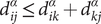 ), non‑negativity (
$ {d}_{ij}^{\alpha}\ge 0 $
), non‑negativity (
$ {d}_{ij}^{\alpha}\ge 0 $
 ), and standardization of distances to the interval
$ 0\le {d}_{ij}^{\alpha}\le 1 $
), and standardization of distances to the interval
$ 0\le {d}_{ij}^{\alpha}\le 1 $
 (Ricotta and Szeidl, Reference Ricotta and Szeidl2006).
Note that RQID reduces to the GSID [Eq. (9)] in the case where all
$ {d}_{ij}^{\alpha } $
 takes the value 0 or 1, i.e., the distance variable between two ideas is binary-valued. Detailed mathematical proof regarding the unbiased estimate of Rao’s quadratic diversity index and its relationship with the GSI can be found in Chen et al. (Reference Chen, Wu and Shen2018).
Now, considering all abstraction levels (i.e., α = 1…m), the weighted average variety of an individual concept
$ V\left({C}_i\right) $
 and the concept space
$ V(C) $
and the concept space
$ V(C) $
 as a whole can be calculated as follows:


Similarly, we can also get a weighted average distance matrix
$ D(C)={\left[{D}_{ij}\right]}_{N\times N} $
 for the concept space
$ C $
for the concept space
$ C $
 considering all abstraction levels, where an element
$ {D}_{ij} $
considering all abstraction levels, where an element
$ {D}_{ij} $
 of the matrix
$ D(C) $
of the matrix
$ D(C) $
 is calculated as follows:

The weights (
$ {w}_{\alpha } $
 ) of different abstraction levels can be assigned to reflect the relative importance of each level. Higher weights can be used for abstraction levels where differences between concepts are considered more significant, resulting in a higher variety score for the concept space. In practice, these weights can be defined by the user in the database sheet according to the design problem and the intended emphasis on particular abstraction levels. However, finding an optimized set of weights requires further research, which is outside this article’s scope.
Computer implementation
A software tool – called VariAnT (Variety Assessment Tool) – has been developed to automate the assessment process. The tool’s Graphical User Interface (GUI) is created with the PySimpleGUI (https://www.pysimplegui.org/) Python library and is shown in Figure 12. The GUI consists of the following six panels:
-
1. The user can create an Excel file consisting of the concept space information (i.e., $ {S}_i,i=1\dots N $
) of all the concepts (i.e.,
$ {C}_i,i=1\dots N $
) of a concept space (i.e.,
$ C $
with
$ N $
concepts). This file can be imported into the tool data frame using the Import Data panel. In the current implementation, the weights for each abstraction level must be specified in brackets as numeric values alongside the abstraction level headings (e.g., “physical principle (10)”). -
2. Once the data is imported into the tool, the user can use the Concept space panel to display the current data frame. This panel displays the data frame where each row corresponds to a particular description (i.e., $ {e}_i^{\alpha k} $
) of a concept
$ {C}_i $
. -
3. VariAnT allows the user to choose a vector encoding method, e.g., S-BERT, as discussed in Section “Vector encoding.” The user can initiate the assessment process by clicking the Calculate Variety button. The tool enables users to apply uniform weights or customize the weight values for different abstraction levels through a checkbox.
-
4. Once the calculations are done, the variety score of the concept space, i.e., $ V\;(C) $
[see Eq. (17)], is displayed in the Results panel. In addition to the
$ V\;(C) $
score, the tool generates four different plots to provide more insights to the user. These plots are discussed in detail in the following section.Figure 12.VariAnT user interface.
Figure 12. Long description
The interface is titled VariAnT v 1 dot 3 dot 7 at the top center.
Top-Left Zone: Import data section. It contains a file path text box with a Browse button, a Read Excel file button, and a Select Method dropdown menu currently set to Cosine distance (S - B E R T). Below this is a checkbox for Use weighted average and a Calculate Variety button. An external label points to this area as Import DataFrame and Select Feature Extraction Method.
Top-Right Zone: Results section. It displays a Variety Score of The Concept Space of 0.6274. Below this are four buttons labeled Plot 1 for Individual Variety Scores, Plot 2 for Variety Scores at Different Levels of Abstraction, Plot 3 for Distance Matrix, and Plot 4 for Hierarchical Relationship Between Concepts. An external label points to this area as Display Results.
Bottom Zone: Concept space section. It includes Show Database and Clear Database buttons above a large data table. The table has five columns: Concept I D, Instance I D, Physical Principle, Working Principle, and Embodiment. The table lists ten concepts. Concepts 1 through 3 use Sliding as the physical principle. Concepts 4 through 7 use Gripping. Concepts 8 through 10 use Rolling. Embodiments include Skis, Snowboard, Sled, Snow Shoes, Other features, Hands, Crank, Wheels, Treads, and Conveyor. An external label points to this table as Display DataFrame.


Demonstration and evaluation of the proposed framework with example cases
Variety assessment of design concepts represented using SAPPhIRE abstraction levels
To demonstrate the proposed variety assessment framework, a synthetic concept space (
$ {C}^W $
 ,
$ N=4 $
,
$ N=4 $
 ) is considered, which consists of four concepts generated using the web interface of ChatGPT (https://chatgpt.com/). We have used the GPT-4o model with default settings. The concepts were generated in response to the following design problem: “How to boil water?” The model was asked to provide four concepts and explicitly describe them using seven abstraction levels of SAPPhIRE, adhering to the definitions of SAPPhIRE constructs. The prompting strategy used for this purpose is outside this article’s scope and is discussed elsewhere (Majumder et al., Reference Majumder, Bhattacharya and Chakrabarti2025). The concepts generated and corresponding SAPPhIRE constructs are given in Table 1. Now, given the SAPPhIRE descriptions of the four concepts of the concept space
$ {C}^W $
) is considered, which consists of four concepts generated using the web interface of ChatGPT (https://chatgpt.com/). We have used the GPT-4o model with default settings. The concepts were generated in response to the following design problem: “How to boil water?” The model was asked to provide four concepts and explicitly describe them using seven abstraction levels of SAPPhIRE, adhering to the definitions of SAPPhIRE constructs. The prompting strategy used for this purpose is outside this article’s scope and is discussed elsewhere (Majumder et al., Reference Majumder, Bhattacharya and Chakrabarti2025). The concepts generated and corresponding SAPPhIRE constructs are given in Table 1. Now, given the SAPPhIRE descriptions of the four concepts of the concept space
$ {C}^W $
 , the variety assessment is carried out using the software tool. The following text embedding model is used: “all-MiniLM-L6-v2”; and the weights (
$ {w}_{\alpha } $
, the variety assessment is carried out using the software tool. The following text embedding model is used: “all-MiniLM-L6-v2”; and the weights (
$ {w}_{\alpha } $
 ) of different abstraction levels are arbitrarily assigned as:
$ {w}_1=7 $
) of different abstraction levels are arbitrarily assigned as:
$ {w}_1=7 $
 (Actions),
$ {w}_2=6 $
(Actions),
$ {w}_2=6 $
 (States),
$ {w}_3=5 $
(States),
$ {w}_3=5 $
 (Inputs),
$ {w}_4=4 $
(Inputs),
$ {w}_4=4 $
 (Phenomena),
$ {w}_5=3 $
(Phenomena),
$ {w}_5=3 $
 (Effects),
$ {w}_6=2 $
(Effects),
$ {w}_6=2 $
 (oRgans),
$ {w}_7=1 $
(oRgans),
$ {w}_7=1 $
 (Parts). The weightage values are adapted from Srinivasan and Chakrabarti (Reference Srinivasan and Chakrabarti2010a). The rationale is to obtain a higher variety score for a given concept space where the concepts differ at a higher abstraction level. The results obtained from the tool are discussed as follows.
Variety assessment results
The variety score of the concept space as a whole is calculated as
$ V\;\left({C}^W\right)=\hskip0.15em 0.378 $
 . The individual variety scores (
$ V\;\left({C}_i\right),i=1\dots 4 $
. The individual variety scores (
$ V\;\left({C}_i\right),i=1\dots 4 $
 ) are exported as a bar chart from the tool, as shown in Figure 13a. Here, the friction heater’s individual variety score,
$ V\;\left({C}_4^W\right)=\hskip0.15em 0.46 $
) are exported as a bar chart from the tool, as shown in Figure 13a. Here, the friction heater’s individual variety score,
$ V\;\left({C}_4^W\right)=\hskip0.15em 0.46 $
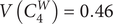 , is the highest compared to other concepts. This interpretation aligns with the notion of “a-posteriori” where a concept’s distinctiveness is defined relative to the set it belongs to, as discussed in Fiorineschi et al. (Reference Fiorineschi, Frillici and Rotini2022).
Results obtained for the concept space
$ {C}^W $
 : (a) Individual variety scores; (b) variety scores of the concept space at different levels of abstraction; (c) the weighted average distances between each pair of concepts; and (d) dendrogram generated from the clustering results.

Figure 13. Long description
Panel a is a bar chart titled Individual Variety Scores. The y-axis is V(C sub i) from 0.0 to 0.4. Four teal bars represent: Electric Kettle at 0.31, Gas Stove with Kettle at 0.37, Solar Water Heater at 0.37, and Friction Heater at 0.46.
Panel b is a box plot titled Variety Scores at Different Levels of Abstraction. The y-axis is V sub i super alpha from 0.0 to 0.8. The x-axis lists Actions, States, Inputs, Phenomena, Effects, oRgans, and Parts. Red dots highlight outliers: Friction Heater at 0.49 in Actions, Friction Heater at 0.07 in States, and Electric Kettle at 0.62 in Inputs.
Panel c is a heat map titled Weighted Average Distance Matrix D(C). The x and y axes list Electric Kettle, Gas Stove with Kettle, Solar Water Heater, and Friction Heater. The color scale ranges from yellow (0.0) to dark green (1.0). The diagonal from bottom-left to top-right shows 0.000 values. The highest distance is 0.503 between Solar Water Heater and Friction Heater.
Panel d is a Dendrogram. The x-axis is Distance from 0.5 to 0.0. Solar Water Heater and Electric Kettle cluster first at a distance of approximately 0.26. This group then clusters with Gas Stove with Kettle at approximately 0.34. Finally, Friction Heater joins the cluster at a distance of approximately 0.53.
Figure 13b shows the variety score of the concept space (
$ {C}^W $
 ) at an abstraction level
$ \alpha $
) at an abstraction level
$ \alpha $
 , i.e.,
$ {V}^{\alpha}\left({C}^W\right) $
, i.e.,
$ {V}^{\alpha}\left({C}^W\right) $
 [see Eq. (15)]. In this figure,
$ {V}^{\alpha}\left({C}^W\right) $
[see Eq. (15)]. In this figure,
$ {V}^{\alpha}\left({C}^W\right) $
 (
$ =\overline{V_i^{\alpha }} $
(
$ =\overline{V_i^{\alpha }} $
 ) score, depicted in the box plot, is represented by a horizontal orange line inside the box, providing a visual indication of the central tendency of the
$ {V}_i^{\alpha } $
) score, depicted in the box plot, is represented by a horizontal orange line inside the box, providing a visual indication of the central tendency of the
$ {V}_i^{\alpha } $
 scores [see Eq. (14)]. Here, outliers are shown in red circles. At a particular abstraction level, these outlier values indicate which concept(s) significantly varied from the other concepts. For example, Figure 13b shows that at the State change level,
$ {V}_i^{\alpha = states} $
scores [see Eq. (14)]. Here, outliers are shown in red circles. At a particular abstraction level, these outlier values indicate which concept(s) significantly varied from the other concepts. For example, Figure 13b shows that at the State change level,
$ {V}_i^{\alpha = states} $
 score of the friction heater is higher compared to the other 3 concepts. Srinivasan and Chakrabarti (Reference Srinivasan and Chakrabarti2010a) conducted observational studies involving an individual designer in each design session to solve a conceptual design problem. The objective was to test whether “an increase in the size and variety of ideas used while designing should enhance the variety of concepts produced, leading to an increase in the novelty of the concept space.” They concluded that a more diverse set of ideas generated at a higher abstraction level leads to a greater chance of producing a newer concept. Thus, examining the variety score across different levels of abstraction, as shown in Figure 13b, may provide valuable insights into the idea-space exploration. For example, while synthesizing concepts, a designer or design team can focus on the abstraction level with a low variety score and try to diversify the ideas in that particular idea space.
Figure 13c shows a heatmap of the weighted average distances (
$ {D}_{ij} $
 ) between each pair of concepts (
$ {C}_i^W,{C}_j^W $
) between each pair of concepts (
$ {C}_i^W,{C}_j^W $
 ) where,
$ i,j=1\dots 4 $
) where,
$ i,j=1\dots 4 $
 . Using these pairwise distance values, the tool can perform clustering where the user defines the number of clusters. Once the number of clusters is defined, the tool implements the K-means clustering algorithm and prints the resulting cluster labels. Additionally, it generates a dendrogram from the clustering results, as shown in Figure 13d. This plot helps to visualize sets of concepts that are similar to each other. Researchers argued that it is easier to explore a large concept space meaningfully when designers browse a clustered concept space because they only need to go through a few concepts from each cluster to get a fair overview, instead of going through every concept (Langdon and Chakrabarti, Reference Langdon and Chakrabarti1999).
Comparative evaluation with existing methods
Here, we evaluate the proposed framework against the existing methods discussed in Section “Existing variety metrics in engineering design.” To demonstrate practical applicability – unlike the synthetic concept space used previously – we employ ideas generated from a real ideation exercise reported by Henderson et al. (Reference Henderson, Helm, Jablokow, McKilligan, Daly and Silk2017). The problem brief, discussed in detail in their study, concerns generating concepts for transportation in snowy environments. The concepts used in this evaluation are listed in Table 2.
The first 16 concepts in Table 2, denoted as
$ {C}_i^T,i=\mathrm{1}\dots \mathrm{16} $
 , are taken directly from Henderson et al. (Reference Henderson, Helm, Jablokow, McKilligan, Daly and Silk2017). To facilitate comparative evaluation, seven additional concepts, i.e.,
$ {C}_i^T,i=\mathrm{17}\dots \mathrm{23} $
, are taken directly from Henderson et al. (Reference Henderson, Helm, Jablokow, McKilligan, Daly and Silk2017). To facilitate comparative evaluation, seven additional concepts, i.e.,
$ {C}_i^T,i=\mathrm{17}\dots \mathrm{23} $
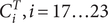 , were created and appended to the original set.
Importantly, if we divide the concept space
$ {C}^T $
 into two sets: Set P (
$ {C}_i^T,i=\mathrm{1}\dots \mathrm{16} $
into two sets: Set P (
$ {C}_i^T,i=\mathrm{1}\dots \mathrm{16} $
 ) and Set Q (
$ {C}_i^T,i=\mathrm{8}\dots \mathrm{23} $
) and Set Q (
$ {C}_i^T,i=\mathrm{8}\dots \mathrm{23} $
 ), both the sets result in identical genealogy trees (refer to Section “An example concept space and its genealogy tree”). Consequently, all the existing variety assessment methods, discussed in Section “Existing variety metrics in engineering design,” would assign identical variety scores to both sets. However, it is evident from the underlying data that, at the level of physical principles, the ideas in Set Q are conceptually more heterogeneous than those in Set P. A reliable variety assessment method should be capable of capturing this distinction. Without this sensitivity, variety would collapse into a mere count of ideas, capturing only fluency, and the distinction between fluency and variety as two separate creativity measures would effectively disappear. Therefore, detecting conceptual distance at different abstraction levels is fundamental to preserving the theoretical integrity and practical usefulness of variety as a metric.
When the data for Sets P and Q are processed using the proposed tool, the resulting variety scores are 0.627 and 0.692, respectively. These results were obtained using the “all-MiniLM-L6-v2” text embedding model and the following user-defined abstraction-level weights (
$ {w}_{\alpha } $
 ):
$ {w}_1=10 $
):
$ {w}_1=10 $
 (physical principle),
$ {w}_2=6 $
(physical principle),
$ {w}_2=6 $
 (working principle), and
$ {w}_3=3 $
(working principle), and
$ {w}_3=3 $
 (embodiment). The increase in the score for Set Q demonstrates the sensitivity of the proposed framework to conceptual differences at higher abstraction levels and also illustrates its adaptability to different knowledge representation schemes.
Limitations of the proposed framework and tool
Following are some of the limitations of the proposed framework and the current implementation of the “VariAnT” tool:
-
1. The current algorithm has a computational complexity of $ O\left({N}^2\right) $
, where
$ N $
is the number of concepts. As the number of concepts or abstraction levels increases, the computation time may grow significantly. However, this problem can be mitigated by utilizing parallel computing, which is currently not implemented in the tool. -
2. Generating text embeddings can be time-consuming or costly, depending on the embedding model used and the computational resources available. Larger models or embeddings with higher dimensionality may require longer processing times.
-
3. The current tool does not include methods for optimizing the selection of concepts to maximize variety. For example, in a design-by-analogy tool, e.g., IDEA-INSPIRE (Chakrabarti et al., Reference Chakrabarti, Siddharth, Dinakar, Panda, Palegar and Keshwani2017), one could identify n stimuli from a total of N concepts such that the variety of the selected subset is maximized. Similar functionality was addressed by Ahmed et al. (Reference Ahmed, Ramachandran, Fuge, Hunter and Miller2021) where a greedy algorithm was implemented, and the same can be implemented in “VariAnT” as well in the future.
-
4. The tool currently operates only on concept spaces represented in textual form. Extending the framework to handle sketches, images, or CAD models would require the use of image embedding or 3D feature embedding methods, but the underlying framework would remain the same. Implementation for non-textual inputs is planned for future work.
-
5. The accuracy of the variety assessment depends on the quality and consistency of the textual descriptions of concepts. In the demonstrations presented, concept descriptions were assumed to be accurate and consistent. Issues such as spelling errors, factual inaccuracies, or inconsistent descriptions are not automatically corrected by the tool and rely on careful user input.
-
6. The usability of VariAnT has not been evaluated in real-world design scenarios with designers. This aspect is beyond the scope of the current study but represents an important direction for future research.


Conclusions and future work
This article reviewed several existing metrics from the engineering design literature that were proposed to quantify the variety of design concept spaces. It was found that most of the existing variety metrics employ a genealogy tree-based approach. Two test cases were conducted to highlight the limitations of these existing variety metrics. The metrics were evaluated in terms of accuracy and sensitivity. Here, the term “accuracy” denotes the validity of a metric; “sensitivity” indicates the ability of a metric to reflect a change in measurement with varying numbers of concepts in a concept space, as well as the distribution of concepts over the nodes of their genealogy tree. Results from two test cases suggested that the “bias-corrected” GSID was better for assessing the variety of a concept space than the other existing metrics. It was found that a major assumption underlying all these metrics is that the ideas in the idea space are considered equally distant. However, in practice, a real-valued distance can be obtained between two different concepts at a particular abstraction level.
To address this research gap, a new prescriptive framework has been proposed for assessing the variety score of a concept space. One of the distinct features of the proposed framework is the use of the SAPPhIRE model of causality as a knowledge representation scheme, which resolves the problem of representing complex systems. The other significant advantage of the framework is using the RQID as a variety metric, which enables us to use real-valued pairwise distances instead of creating a genealogy tree. It was found that RQID reduces to the GSID if the distance variable between two ideas is binary-valued, i.e., 0 or 1. Hence, the proposed metric, by default, qualifies for a genealogy tree-based variety assessment. We have also discussed a step-by-step approach to measure the distance between two design concepts by comparing their respective textual descriptions. The proposed variety assessment framework was embodied into a new software tool called “VariAnT.” The tool provides a GUI and automates the proposed variety assessment process. Finally, the tool was tested with an example concept space, and the results obtained from the tool were discussed.
There are three potential research directions in the future: (a) Besides S-BERT, it is also possible to incorporate several alternative vector encoding methods into the framework, such as OpenAI embeddings and universal-sentence-encoder. Thus, finding the most appropriate method or combination of methods that correlate better with expert variety score ratings requires an empirical investigation; (b) In this work, the weights of different abstraction levels have been assigned arbitrarily, where the highest importance is given to the function followed by behavior and structure. Therefore, additional optimization algorithms can be incorporated to optimize the set of weights that can maximize the sensitivity or discriminating power of the proposed framework; (c) Lastly, apart from assessing the variety, the proposed framework could also be integrated with existing “design-by-analogy” or “analogy retrieval” tools, such as IDEA-INSPIRE (Chakrabarti et al., Reference Chakrabarti, Siddharth, Dinakar, Panda, Palegar and Keshwani2017) and DANE (Vattam et al., Reference Vattam, Wiltgen, Helms, Goel and Yen2011), so as to provide insights into the variety of the analogy space retrieved by the tool. The proposed method could also be utilized to control analogical distance while performing a search.
Data availability statement
The authors confirm that all data generated or analyzed during this study are included in this article.
Competing interest
The authors declare that they have no known competing financial interests or personal relationships that could have appeared to influence the work reported in this article.


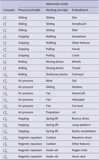
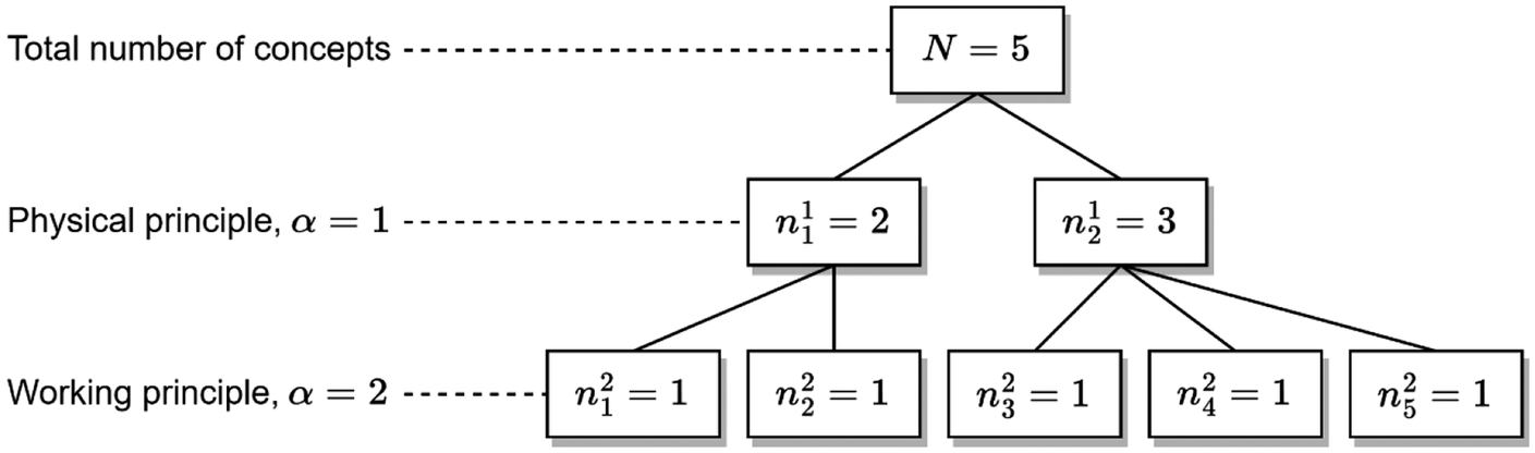

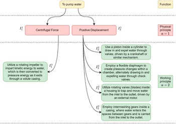

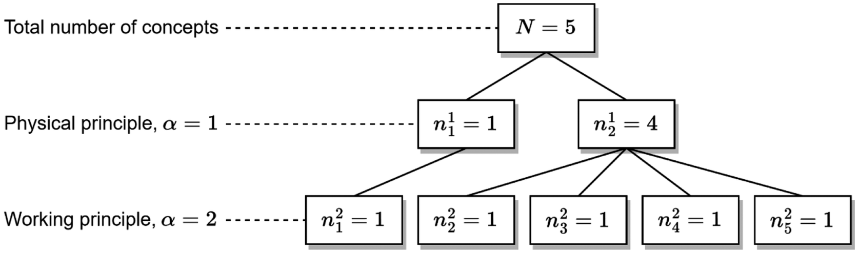


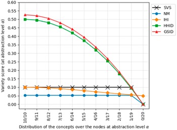
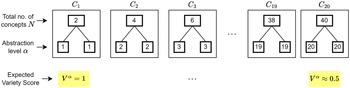
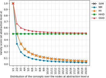
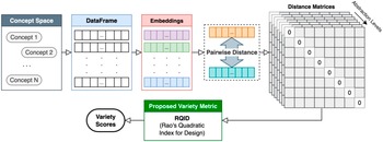

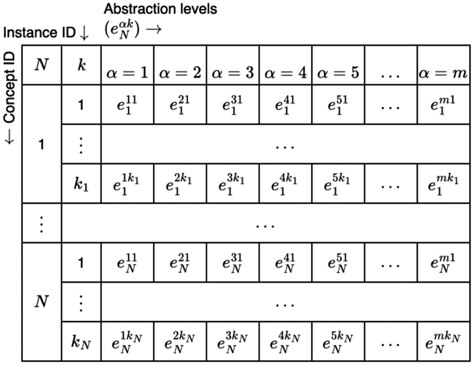

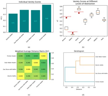


 Open access

