













1. Introduction
Let $G$
be a connected simple real algebraic group of rank one and
$G$
be a connected simple real algebraic group of rank one and $(X, \mathsf{d})$
the associated Riemannian symmetric space so that
$(X, \mathsf{d})$
the associated Riemannian symmetric space so that $G=\operatorname {Isom}^+(X)$
. Let
$G=\operatorname {Isom}^+(X)$
. Let $\Gamma$
be a non-elementary convex-cocompact subgroup of
$\Gamma$
be a non-elementary convex-cocompact subgroup of $G$
. Denote by
$G$
. Denote by $[\Gamma ]$
the conjugacy classes of elements of
$[\Gamma ]$
the conjugacy classes of elements of $\Gamma$
. To each non-trivial element
$\Gamma$
. To each non-trivial element $[\gamma ]\in [\Gamma ]$
corresponds a unique closed geodesic in the locally symmetric manifold
$[\gamma ]\in [\Gamma ]$
corresponds a unique closed geodesic in the locally symmetric manifold $\Gamma {\backslash } X$
whose length we denote by
$\Gamma {\backslash } X$
whose length we denote by $\ell _\gamma$
. Let
$\ell _\gamma$
. Let $\delta _{\Gamma} \gt 0$
denote the critical exponent of
$\delta _{\Gamma} \gt 0$
denote the critical exponent of $\Gamma$
. The prime geodesic theorem and orbital counting theorem say that, as
$\Gamma$
. The prime geodesic theorem and orbital counting theorem say that, as $T \to \infty$
,
$T \to \infty$
,
 \begin{align} \#\{[\gamma ]\in [\Gamma ]: \ell _{\gamma } \le T\} \sim \frac {e^{\delta _{\Gamma} T}}{\delta _{\Gamma} T} ; \end{align}
andFootnote 1
 \begin{align} \#\{ \gamma \in \Gamma : \mathsf{d}(\gamma o,o) \le T\} \sim \frac {e^{\delta _{\Gamma} T}}{|m^{\operatorname {BMS}}|\delta _{\Gamma} } \end{align}
where $o\in X$
and
$o\in X$
and $m^{\operatorname {BMS}}$
denote the suitably normalized Bowen–Margulis–Sullivan measure on the unit tangent bundle of
$m^{\operatorname {BMS}}$
denote the suitably normalized Bowen–Margulis–Sullivan measure on the unit tangent bundle of $\Gamma \backslash X$
. This is due to Margulis [Reference MargulisMar04] and Roblin [Reference RoblinRob03] in this generality (see also [Reference HuberHub59, Reference Gangolli and WarnerGW80]). We identify the unit tangent bundle of
$\Gamma \backslash X$
. This is due to Margulis [Reference MargulisMar04] and Roblin [Reference RoblinRob03] in this generality (see also [Reference HuberHub59, Reference Gangolli and WarnerGW80]). We identify the unit tangent bundle of $\Gamma \backslash X$
with
$\Gamma \backslash X$
with $\Gamma \backslash G/M$
where
$\Gamma \backslash G/M$
where $M$
is a compact subgroup of
$M$
is a compact subgroup of $G$
. For each non-trivial
$G$
. For each non-trivial $[\gamma ]\in [\Gamma ]$
, there exists a unique conjugacy class
$[\gamma ]\in [\Gamma ]$
, there exists a unique conjugacy class $[m_\gamma ]$
of
$[m_\gamma ]$
of $M$
, called the holonomy of
$M$
, called the holonomy of $\gamma$
. Equidistribution of holonomies was obtained for lattices by Sarnak and Wakayama [Reference Sarnak and WakayamaSW99], and the following joint equidistribution was proved by Margulis, Mohammadi and Oh [Reference Margulis, Mohammadi and OhMMO14] for all Zariski dense convex-cocompact
$\gamma$
. Equidistribution of holonomies was obtained for lattices by Sarnak and Wakayama [Reference Sarnak and WakayamaSW99], and the following joint equidistribution was proved by Margulis, Mohammadi and Oh [Reference Margulis, Mohammadi and OhMMO14] for all Zariski dense convex-cocompact $\Gamma$
: for any conjugation-invariant Borel subset
$\Gamma$
: for any conjugation-invariant Borel subset $\Theta \subset M$
with smooth boundary, as
$\Theta \subset M$
with smooth boundary, as $T\to \infty$
,
$T\to \infty$
,
 \begin{align} \#\{[\gamma ]\in [\Gamma ]: \ell _{\gamma } \le T, m_\gamma \in \Theta \} \sim \frac {e^{\delta _{\Gamma} T}}{\delta _{\Gamma} T}\operatorname {Vol}_M(\Theta ) \end{align}
where $\operatorname {Vol}_M$
denotes the Haar probability measure on
$\operatorname {Vol}_M$
denotes the Haar probability measure on $M$
.
$M$
.
Correlations of spectra
For a finitely generated group $\Gamma$
Footnote
2
and a
$\Gamma$
Footnote
2
and a $d$
-tuple of faithful Zariski-dense convex-cocompact representations
$d$
-tuple of faithful Zariski-dense convex-cocompact representations
 \begin{align*} \rho =(\rho _1, \ldots , \rho _d) :\Gamma \to G,\end{align*}
we are interested in understanding the correlations among the length spectra $\{\ell _{\rho _i(\gamma )}: [\gamma ]\in [\Gamma ]\}$
and holonomies and the correlations among the displacement spectra
$\{\ell _{\rho _i(\gamma )}: [\gamma ]\in [\Gamma ]\}$
and holonomies and the correlations among the displacement spectra $\{\mathsf{d}(\rho _i(\gamma ) o,o):\gamma \in \Gamma \}$
,
$\{\mathsf{d}(\rho _i(\gamma ) o,o):\gamma \in \Gamma \}$
, $i=1,\ldots , d$
. These correlations are restricted by the spectrum cone
$i=1,\ldots , d$
. These correlations are restricted by the spectrum cone $\mathcal L_\rho$
, which is the smallest closed cone in
$\mathcal L_\rho$
, which is the smallest closed cone in ${\mathbb R}^d$
containing all vectors
${\mathbb R}^d$
containing all vectors $(\ell _{\rho _1(\gamma )},\ldots ,\ell _{\rho _d(\gamma )})$
,
$(\ell _{\rho _1(\gamma )},\ldots ,\ell _{\rho _d(\gamma )})$
, $[\gamma ]\in [\Gamma ]$
. The interior
$[\gamma ]\in [\Gamma ]$
. The interior $\textrm {int}{\mathcal L}_\rho$
is non-empty if and only if
$\textrm {int}{\mathcal L}_\rho$
is non-empty if and only if $\rho _1,\ldots ,\rho _d$
are independent from each other in the sense that no
$\rho _1,\ldots ,\rho _d$
are independent from each other in the sense that no $\rho _i\circ \rho _j^{-1}:\rho _j(\Gamma )\to \rho _i(\Gamma )$
extends to a Lie group automorphism of
$\rho _i\circ \rho _j^{-1}:\rho _j(\Gamma )\to \rho _i(\Gamma )$
extends to a Lie group automorphism of $G$
for all
$G$
for all $i\ne j$
(cf. proof of Theorem7.1).
$i\ne j$
(cf. proof of Theorem7.1).
Theorem 1.1.
Let $\Gamma$
be a finitely generated group and
$\Gamma$
be a finitely generated group and $d\in \mathbb N$
. Let
$d\in \mathbb N$
. Let $\rho =(\rho _1, \ldots , \rho _d):\Gamma \to G$
be a
$\rho =(\rho _1, \ldots , \rho _d):\Gamma \to G$
be a $d$
-tuple of faithful Zariski-dense convex-cocompact representations. For any vector
$d$
-tuple of faithful Zariski-dense convex-cocompact representations. For any vector ${\mathsf v} =(v_1, \ldots , v_d) \in \operatorname {int} {\mathcal L}_\rho$
, there exists
${\mathsf v} =(v_1, \ldots , v_d) \in \operatorname {int} {\mathcal L}_\rho$
, there exists $\delta _\rho ({\mathsf v})\gt 0$
such that for any
$\delta _\rho ({\mathsf v})\gt 0$
such that for any ${\varepsilon }_1,\ldots ,{\varepsilon }_d\gt 0$
and for any conjugation-invariant Borel sets
${\varepsilon }_1,\ldots ,{\varepsilon }_d\gt 0$
and for any conjugation-invariant Borel sets $\Theta _1, \ldots , \Theta _d \subset M$
with null boundaries, we have as
$\Theta _1, \ldots , \Theta _d \subset M$
with null boundaries, we have as $T\to \infty$
,
$T\to \infty$
,
 \begin{align*} \#\{[\gamma ]\in [\Gamma ]: v_iT \le \ell _{\rho _i(\gamma )} \le v_iT+{\varepsilon }_i,\, m_{\rho _i(\gamma )}\in \Theta _i, \; 1\le i\le d\} \\ \sim c \frac {e^{\delta _\rho ({\mathsf v})T}}{ T^{(d+1)/{2}}} \prod _{i=1}^d\operatorname {Vol}_{M}(\Theta _i) \end{align*}
and
 \begin{align*} & \#\{\gamma \in \Gamma : v_iT \le {\mathsf d} ({\rho _i(\gamma )}o, o) \le v_iT+{\varepsilon }_i, \; 1 \le i \le d \} \sim c\cdot c' \cdot \frac {e^{{\delta }_\rho ({\mathsf v})T}}{ T^{{(d-1)}/{2}}} \end{align*}
for some constants $c =c({\mathsf v}, {\varepsilon }_1,\ldots ,{\varepsilon }_d) \gt 0$
and
$c =c({\mathsf v}, {\varepsilon }_1,\ldots ,{\varepsilon }_d) \gt 0$
and $c'=c'({\mathsf v})\gt 0$
.
$c'=c'({\mathsf v})\gt 0$
.
Moreover,
 \begin{align} \delta _\rho ({\mathsf v}) \le \min _i \delta _{\rho _i(\Gamma )}v_i. \end{align}
If $d\ge 2$
, we also have
$d\ge 2$
, we also have
 \begin{align} \delta _\rho ({\mathsf v})\lt \frac {1}{d} \sum _{i=1}^d \delta _{\rho _i(\Gamma )} v_i . \end{align}
The $d=2$
case: note that the size of the box is independent of
$d=2$
case: note that the size of the box is independent of $T$
.
$T$
.

Remark 1.2.
-
1. Let $\Gamma$
be a cocompact lattice of
$\operatorname {PSL}_2(\mathbb R)=\operatorname {Isom}^+(\mathbb H^2)$
and
$\rho :\Gamma \to \operatorname {PSL}_2{\mathbb R}$
a discrete faithful representation (whose image is necessarily a cocompact lattice). Letbe the minimal and maximal stretch constants of
\begin{align*} \mathsf m_\rho =\inf _{\gamma \in \Gamma -\{e\}} \frac {\ell _{\rho (\gamma )}}{\ell _\gamma } \quad \textrm{and} \quad \mathsf M_\rho = \sup _{\gamma \in \Gamma -\{e\}} \frac {\ell _{\rho (\gamma )}}{\ell _\gamma } \end{align*}
$\rho$
respectively. By a theorem of Thurston [Reference ThurstonThu22, Theorem 3.1], if
$\rho$
is not a conjugation by a Möbius transformation, then
$\mathsf m_\rho \lt 1\lt \mathsf M_\rho$
. In this case, the first asymptotic on the correlations of length spectra in Theorem 1.1 for the pair
$(\textrm{id}, \rho )$
was proved by Schwartz and Sharp [Reference Schwartz and SharpSS93, Theorem 1] for the specific direction
${\mathsf v}=(1,1)$
together with the bound
$\delta _{(\textrm{id}, \rho )} (1,1)\lt 1$
. We also mention a related work by Dai and Martone [Reference Dai and MartoneDM22] which generalizes the result from Schwartz and Sharp to pairs of Hitchin representations and some specific direction. Their results do not overlap with our results.
$\Gamma$
be a cocompact lattice of
$\operatorname {PSL}_2(\mathbb R)=\operatorname {Isom}^+(\mathbb H^2)$
and
$\rho :\Gamma \to \operatorname {PSL}_2{\mathbb R}$
a discrete faithful representation (whose image is necessarily a cocompact lattice). Letbe the minimal and maximal stretch constants of
\begin{align*} \mathsf m_\rho =\inf _{\gamma \in \Gamma -\{e\}} \frac {\ell _{\rho (\gamma )}}{\ell _\gamma } \quad \textrm{and} \quad \mathsf M_\rho = \sup _{\gamma \in \Gamma -\{e\}} \frac {\ell _{\rho (\gamma )}}{\ell _\gamma } \end{align*}
$\rho$
respectively. By a theorem of Thurston [Reference ThurstonThu22, Theorem 3.1], if
$\rho$
is not a conjugation by a Möbius transformation, then
$\mathsf m_\rho \lt 1\lt \mathsf M_\rho$
. In this case, the first asymptotic on the correlations of length spectra in Theorem 1.1 for the pair
$(\textrm{id}, \rho )$
was proved by Schwartz and Sharp [Reference Schwartz and SharpSS93, Theorem 1] for the specific direction
${\mathsf v}=(1,1)$
together with the bound
$\delta _{(\textrm{id}, \rho )} (1,1)\lt 1$
. We also mention a related work by Dai and Martone [Reference Dai and MartoneDM22] which generalizes the result from Schwartz and Sharp to pairs of Hitchin representations and some specific direction. Their results do not overlap with our results.
-
2. If we set
$\ell _{\rho (\gamma )} = (\ell _{\rho _1(\gamma )}, \ldots , \ell _{\rho _d(\gamma )})$
, then the condition
$v_iT \le \ell _{\rho _i(\gamma )} \le v_iT +{\varepsilon }_i$
,
$1 \le i \le d$
, can be written as
$\ell _{\rho (\gamma )} \in T{\mathsf v} + \prod _{i=1}^d[0,{\varepsilon }_i]$
(cf. Figure 1). We remark that if we replace the box
$\prod _{i=1}^d[0,{\varepsilon }_i]$
with a general compact set
$\mathcal K$
with null boundary, then we can approximate
$\mathcal K$
with boxes and we obtain the same asymptotic in Theorem 1.1 with constant
$c = c({\mathsf v}, \mathcal K)$
. Similarly for displacements.












Correlation of complex eigenvalues
When $G=\operatorname {PSL}_2({\mathbb C})=\operatorname {Isom}^+(\mathbb H^3)$
, Theorem1.1 describes the correlations of complex eigenvalues of convex-cocompact representations. Denote by
$G=\operatorname {PSL}_2({\mathbb C})=\operatorname {Isom}^+(\mathbb H^3)$
, Theorem1.1 describes the correlations of complex eigenvalues of convex-cocompact representations. Denote by $\lambda ^{{\mathbb C}}_g$
the complex eigenvalue of
$\lambda ^{{\mathbb C}}_g$
the complex eigenvalue of $g\in \operatorname {PSL}_2({\mathbb C})$
so that
$g\in \operatorname {PSL}_2({\mathbb C})$
so that $|\lambda _g^{\mathbb C}|\ge 1$
. The argument of
$|\lambda _g^{\mathbb C}|\ge 1$
. The argument of $\lambda ^{{\mathbb C}}_g$
is well-defined as an element of
$\lambda ^{{\mathbb C}}_g$
is well-defined as an element of $[0, \pi )$
, so that
$[0, \pi )$
, so that $\lambda ^{\mathbb C}_g =|\lambda ^{{\mathbb C}}_g| \operatorname {Arg}(\lambda ^{{\mathbb C}}_g)$
. Let
$\lambda ^{\mathbb C}_g =|\lambda ^{{\mathbb C}}_g| \operatorname {Arg}(\lambda ^{{\mathbb C}}_g)$
. Let $\Gamma \lt \operatorname {PSL}_2{\mathbb C}$
be a convex-cocompact subgroup. We have
$\Gamma \lt \operatorname {PSL}_2{\mathbb C}$
be a convex-cocompact subgroup. We have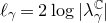 $\ell _{\gamma } = 2\log |\lambda ^{{\mathbb C}}_\gamma |$
for each non-trivial
$\ell _{\gamma } = 2\log |\lambda ^{{\mathbb C}}_\gamma |$
for each non-trivial $\gamma \in \Gamma$
. Since
$\gamma \in \Gamma$
. Since $\delta _{\Gamma }$
is equal to the Hausdorff dimension
$\delta _{\Gamma }$
is equal to the Hausdorff dimension $\operatorname {dim_H}\Lambda _{\Gamma }$
of the limit set of
$\operatorname {dim_H}\Lambda _{\Gamma }$
of the limit set of $\Gamma$
by Patterson and Sullivan ([Reference PattersonPat76, Reference SullivanSul79]), the following is a special case of Theorem1.1.
$\Gamma$
by Patterson and Sullivan ([Reference PattersonPat76, Reference SullivanSul79]), the following is a special case of Theorem1.1.
Corollary 1.3.
Let $\Gamma \lt \operatorname {PSL}_2({\mathbb C})$
be a Zariski-dense convex-cocompact subgroup and
$\Gamma \lt \operatorname {PSL}_2({\mathbb C})$
be a Zariski-dense convex-cocompact subgroup and $\rho :\Gamma \to \operatorname {PSL}_2({\mathbb C})$
a faithful Zariski-dense convex-cocompact representation. For any
$\rho :\Gamma \to \operatorname {PSL}_2({\mathbb C})$
a faithful Zariski-dense convex-cocompact representation. For any $ \mathsf m_\rho \lt s \lt \mathsf M_\rho$
, there exists
$ \mathsf m_\rho \lt s \lt \mathsf M_\rho$
, there exists
 \begin{align*} 0\lt 2 \delta _s \lt \operatorname {dim_H}\Lambda _{\Gamma} + s \cdot \operatorname {dim_H}\Lambda _{\rho (\Gamma )}, \end{align*}
such that for any ${\varepsilon }_1,{\varepsilon }_2 \gt 0$
, there exists a constant
${\varepsilon }_1,{\varepsilon }_2 \gt 0$
, there exists a constant $c=c(s, {\varepsilon }_1, {\varepsilon }_2)\gt 0$
such that for any
$c=c(s, {\varepsilon }_1, {\varepsilon }_2)\gt 0$
such that for any $0\lt \theta _1\lt \theta _2\lt \pi$
and
$0\lt \theta _1\lt \theta _2\lt \pi$
and $0\lt \theta _1'\lt \theta _2'\lt \pi$
, we have as
$0\lt \theta _1'\lt \theta _2'\lt \pi$
, we have as $t\to \infty$
,
$t\to \infty$
,
 \begin{align*} \#\left \lbrace [\gamma ]\in [\Gamma ] : \begin{array}{@{}l@{}} t \le |\lambda ^{{\mathbb C}}_\gamma | \le (1+{\varepsilon }_1) t, \textrm{Arg} (\lambda ^{{\mathbb C}}_\gamma )\in [\theta _1, \theta _2] ,\\ t^s\le |\lambda ^{{\mathbb C}}_{\rho (\gamma )}| \le (1+{\varepsilon }_2) t^s, \textrm{Arg} (\lambda ^{{\mathbb C}}_{\rho (\gamma )}) \in [\theta _1', \theta _2'] \end{array} \right \rbrace \\ \sim c \frac {t^{ 2\delta _s}}{(\log t)^{3/2}} (\theta _2-\theta _1)(\theta _2'-\theta _1') . \end{align*}
Using the relation $\cosh \mathsf{d}(go,o) = \|g\|^2$
where
$\cosh \mathsf{d}(go,o) = \|g\|^2$
where $\|g\|$
denotes the Frobenius norm of
$\|g\|$
denotes the Frobenius norm of $g \in \operatorname {PSL}_2{\mathbb C}$
, we can also obtain correlations for Frobenius norms from Theorem1.1.
$g \in \operatorname {PSL}_2{\mathbb C}$
, we can also obtain correlations for Frobenius norms from Theorem1.1.
Jordan and Cartan projections in tubes
In fact, we prove much more general results for Anosov subgroups on (i) joint equidistribution of Jordan projections in tubes and their holonomies, and (ii) equidistribution of Cartan projections in tubes, of which Theorem1.1 is a special case.
Let $G$
be a connected semisimple real algebraic group. Let
$G$
be a connected semisimple real algebraic group. Let $P \lt G$
be a minimal parabolic subgroup with Langlands decomposition
$P \lt G$
be a minimal parabolic subgroup with Langlands decomposition $P=MAN$
where
$P=MAN$
where $N$
is the unipotent radical of
$N$
is the unipotent radical of $P$
,
$P$
, $A$
is a maximal real split torus and
$A$
is a maximal real split torus and $M$
is a maximal compact subgroup of
$M$
is a maximal compact subgroup of $P$
commuting with
$P$
commuting with $A$
. Let
$A$
. Let $\mathfrak g$
and
$\mathfrak g$
and $\mathfrak a$
denote the Lie algebras of
$\mathfrak a$
denote the Lie algebras of $G$
and
$G$
and $A$
respectively, and choose a positive Weyl chamber
$A$
respectively, and choose a positive Weyl chamber ${\mathfrak a}^+$
. Let
${\mathfrak a}^+$
. Let $K$
be a maximal compact subgroup of
$K$
be a maximal compact subgroup of $G$
such that the Cartan decomposition
$G$
such that the Cartan decomposition $G=K (\exp \mathfrak{a}^+) K$
holds. Let
$G=K (\exp \mathfrak{a}^+) K$
holds. Let $\mu :G\to {\mathfrak a}^+$
denote the Cartan projection, that is,
$\mu :G\to {\mathfrak a}^+$
denote the Cartan projection, that is, $\mu (g)$
is the unique element of
$\mu (g)$
is the unique element of ${\mathfrak a}^+$
such that
${\mathfrak a}^+$
such that $g\in K \exp (\mu (g)) K$
for all
$g\in K \exp (\mu (g)) K$
for all $g\in G$
.
$g\in G$
.
A finitely generated subgroup $\Gamma \lt G$
is called an Anosov subgroup with respect to
$\Gamma \lt G$
is called an Anosov subgroup with respect to $P$
if there exists
$P$
if there exists $C\gt 0$
such that for all
$C\gt 0$
such that for all $\gamma \in \Gamma$
,
$\gamma \in \Gamma$
,
 \begin{align*} \alpha (\mu (\gamma )) \ge C|\gamma | -C^{-1}\end{align*}
for all simple roots $\alpha$
of
$\alpha$
of $(\mathfrak g, {\mathfrak a}^+)$
where
$(\mathfrak g, {\mathfrak a}^+)$
where $|\gamma |$
denotes the word length of
$|\gamma |$
denotes the word length of $\gamma$
with respect to a fixed finite set of generators of
$\gamma$
with respect to a fixed finite set of generators of $\Gamma$
. If we only require this condition for a subset
$\Gamma$
. If we only require this condition for a subset $\theta$
of simple roots, then we get a more general definition of the
$\theta$
of simple roots, then we get a more general definition of the $\theta$
-Anosov subgroup, but this will not be considered in this paper. Anosov subgroups of
$\theta$
-Anosov subgroup, but this will not be considered in this paper. Anosov subgroups of $G$
were first introduced by Labourie [Reference LabourieLab06] for surface groups who showed that the image of a Hitchin representation is Anosov. They were later generalized by Guichard and Wienhard [Reference Guichard and WienhardGW12] for Gromov hyperbolic groups. There are several equivalent characterizations of Anosov subgroups due to Kapovich, Leeb and Porti [Reference Kapovich, Leeb and PortiKLP17], and to Guéritaud, Guichard, Kassel and Wienhard [Reference Guéritaud, Guichard, Kassel and WienhardGGK+17] one of which is given as above. Anosov subgroups are regarded as the higher rank generalization of convex-cocompact subgroups. Schottky subgroups are Anosov and every Zariski-dense subgroup of
$G$
were first introduced by Labourie [Reference LabourieLab06] for surface groups who showed that the image of a Hitchin representation is Anosov. They were later generalized by Guichard and Wienhard [Reference Guichard and WienhardGW12] for Gromov hyperbolic groups. There are several equivalent characterizations of Anosov subgroups due to Kapovich, Leeb and Porti [Reference Kapovich, Leeb and PortiKLP17], and to Guéritaud, Guichard, Kassel and Wienhard [Reference Guéritaud, Guichard, Kassel and WienhardGGK+17] one of which is given as above. Anosov subgroups are regarded as the higher rank generalization of convex-cocompact subgroups. Schottky subgroups are Anosov and every Zariski-dense subgroup of $G$
contains a Schottky, and hence the Anosov subgroup [Reference BenoistBen97]. Another important class of Anosov subgroups which is particularly relevant to this paper is the class of self-joining groups defined in (1.9) associated to a
$G$
contains a Schottky, and hence the Anosov subgroup [Reference BenoistBen97]. Another important class of Anosov subgroups which is particularly relevant to this paper is the class of self-joining groups defined in (1.9) associated to a $d$
-tuple of convex-cocompact representations
$d$
-tuple of convex-cocompact representations $\rho _1, \ldots , \rho _d: \Gamma \to G$
of a finitely generated group
$\rho _1, \ldots , \rho _d: \Gamma \to G$
of a finitely generated group $\Gamma$
.
$\Gamma$
.
In the rest of the introduction, let $\Gamma \lt G$
be a Zariski-dense Anosov subgroup with respect to
$\Gamma \lt G$
be a Zariski-dense Anosov subgroup with respect to $P$
. Every non-trivial element
$P$
. Every non-trivial element $\gamma \in \Gamma$
is loxodromic [Reference Guichard and WienhardGW12, Lemma 3.1] and hence conjugate to an element
$\gamma \in \Gamma$
is loxodromic [Reference Guichard and WienhardGW12, Lemma 3.1] and hence conjugate to an element $\exp (\lambda (\gamma ))m(\gamma )$
where
$\exp (\lambda (\gamma ))m(\gamma )$
where $\lambda (\gamma ) \in \textrm {int}\mathfrak{a}^+$
is the Jordan projection of
$\lambda (\gamma ) \in \textrm {int}\mathfrak{a}^+$
is the Jordan projection of $\gamma$
and
$\gamma$
and $m(\gamma ) \in M$
. The conjugacy class
$m(\gamma ) \in M$
. The conjugacy class $[m(\gamma )]\in [M]$
is uniquely determined and called the holonomy of
$[m(\gamma )]\in [M]$
is uniquely determined and called the holonomy of $\gamma$
. We note that
$\gamma$
. We note that $\lambda (\gamma )$
and
$\lambda (\gamma )$
and $[m(\gamma )]$
depend only on the conjugacy class of
$[m(\gamma )]$
depend only on the conjugacy class of $\gamma$
. The limit cone
$\gamma$
. The limit cone ${\mathcal L}={\mathcal L}_{\Gamma} \subset {\mathfrak a}^+$
of
${\mathcal L}={\mathcal L}_{\Gamma} \subset {\mathfrak a}^+$
of $\Gamma$
is the smallest closed cone containing
$\Gamma$
is the smallest closed cone containing $\lambda (\Gamma )$
; this is a convex cone with non-empty interior [Reference BenoistBen97].
$\lambda (\Gamma )$
; this is a convex cone with non-empty interior [Reference BenoistBen97].
By a tube $\mathbb T$
in
$\mathbb T$
in ${\mathfrak a}^+$
, we mean a subset of the form
${\mathfrak a}^+$
, we mean a subset of the form
 \begin{align*} {\mathbb{T}} ={\mathbb{T}}({\mathsf v}, {\varepsilon }, w)=\{u+w\in {\mathfrak a}^+: \|u-\mathbb R {\mathsf v}\| \le {\varepsilon }\}\end{align*}
for some unit vector ${\mathsf v}\in {\mathfrak a}^+$
,
${\mathsf v}\in {\mathfrak a}^+$
, ${\varepsilon }\gt 0$
, and
${\varepsilon }\gt 0$
, and $w\in {\mathfrak a}$
where
$w\in {\mathfrak a}$
where $\|\cdot \|$
is a Euclidean norm on
$\|\cdot \|$
is a Euclidean norm on $\mathfrak a$
. The unit vector
$\mathfrak a$
. The unit vector $\mathsf v$
will be called the direction of
$\mathsf v$
will be called the direction of $\mathbb{T}$
. We say a tube
$\mathbb{T}$
. We say a tube $\mathbb{T}$
is essential for
$\mathbb{T}$
is essential for $\Gamma$
if its direction
$\Gamma$
if its direction $\mathsf v$
belongs to the interior
$\mathsf v$
belongs to the interior $\operatorname {int} {\mathcal L}$
(cf. Figure 2).
$\operatorname {int} {\mathcal L}$
(cf. Figure 2).
Tube.

The growth indicator $\psi _{\Gamma} : \mathfrak{a}^+ \to [0,\infty ) \cup \{-\infty \}$
of
$\psi _{\Gamma} : \mathfrak{a}^+ \to [0,\infty ) \cup \{-\infty \}$
of $\Gamma$
is defined by
$\Gamma$
is defined by $\psi _{\Gamma} (0)=0$
and
$\psi _{\Gamma} (0)=0$
and

where $\tau _{\mathcal{C}}$
is the abscissa of convergence of the series
$\tau _{\mathcal{C}}$
is the abscissa of convergence of the series $t \mapsto \sum _{\gamma \in \Gamma , \mu (\gamma ) \in \mathcal{C}} e^{-t\|\mu (\gamma )\|}$
. It was first introduced by Quint and it is regarded as the higher rank generalization of the critical exponent in rank one. Quint showed that
$t \mapsto \sum _{\gamma \in \Gamma , \mu (\gamma ) \in \mathcal{C}} e^{-t\|\mu (\gamma )\|}$
. It was first introduced by Quint and it is regarded as the higher rank generalization of the critical exponent in rank one. Quint showed that $\psi _{\Gamma} |_{\mathfrak{a}^+-{\mathcal L}} = -\infty$
,
$\psi _{\Gamma} |_{\mathfrak{a}^+-{\mathcal L}} = -\infty$
, $\psi _{\Gamma} |_{{\mathcal L}}\ge 0$
and
$\psi _{\Gamma} |_{{\mathcal L}}\ge 0$
and $\psi _{\Gamma} |_{\textrm {int}{\mathcal L}}\gt 0$
[Reference QuintQui02, Theorem 4.2.2].
$\psi _{\Gamma} |_{\textrm {int}{\mathcal L}}\gt 0$
[Reference QuintQui02, Theorem 4.2.2].
The holonomy group $M_{\Gamma}$
of
$M_{\Gamma}$
of $\Gamma$
is defined as the smallest closed subgroup of
$\Gamma$
is defined as the smallest closed subgroup of $M$
containing the holonomies of
$M$
containing the holonomies of $\Gamma$
. This is a finite index normal subgroup of
$\Gamma$
. This is a finite index normal subgroup of $M$
[Reference Guivarc’h and RaugiGR07, Corollary 1.10]. We denote by
$M$
[Reference Guivarc’h and RaugiGR07, Corollary 1.10]. We denote by $r=r(G)$
the real rank of
$r=r(G)$
the real rank of $G$
.
$G$
.
Theorem 1.4 (Jordan spectrum). Let $\Gamma \lt G$
be a Zariski-dense Anosov subgroup. For any essential tube
$\Gamma \lt G$
be a Zariski-dense Anosov subgroup. For any essential tube $\mathbb{T}$
of direction
$\mathbb{T}$
of direction $\mathsf v$
, there exists
$\mathsf v$
, there exists $\kappa _{{\mathbb{T}}}\gt 0$
such that for any conjugation-invariant Borel subset
$\kappa _{{\mathbb{T}}}\gt 0$
such that for any conjugation-invariant Borel subset $\Theta \subset M$
with smooth boundary, we have as
$\Theta \subset M$
with smooth boundary, we have as $T\to \infty$
,
$T\to \infty$
,
 \begin{align*} \#\{[\gamma ] \in [\Gamma ]:\|\lambda (\gamma ) \|\le T,\; \lambda (\gamma ) \in {\mathbb{T}},\; m(\gamma )\in \Theta \} \sim \kappa _{{\mathbb{T}}} \frac {e^{\psi _{\Gamma} ({\mathsf v}) T}}{T^{(r+1)/2}} \operatorname {Vol}_M(\Theta \cap M_{\Gamma} ) .\end{align*}
In particular,
 \begin{align*} \#\{[\gamma ] \in [\Gamma ]:\|\lambda (\gamma ) \|\le T,\; \lambda (\gamma ) \in {\mathbb{T}}\} \sim \frac {\kappa _{{\mathbb{T}}}}{[M:M_{\Gamma} ]} \cdot \frac {e^{\psi _{\Gamma} ({\mathsf v}) T}}{T^{(r+1)/2}} . \end{align*}
We also obtain a similar counting result for the Cartan projections $\mu (\Gamma )$
.
$\mu (\Gamma )$
.
Theorem 1.5 (Cartan spectrum). Let $\Gamma \lt G$
be a Zariski-dense Anosov subgroup. For any essential tube
$\Gamma \lt G$
be a Zariski-dense Anosov subgroup. For any essential tube $\mathbb{T}$
of direction
$\mathbb{T}$
of direction $\mathsf v$
, we have as
$\mathsf v$
, we have as $T\to \infty$
,
$T\to \infty$
,
 \begin{align*} \#\{\gamma \in \Gamma :\|\mu (\gamma ) \|\le T,\; \mu (\gamma ) \in {\mathbb{T}}\} \sim \frac {\kappa _{\mathbb{T}}}{|m_{\mathcal{X}_{\mathsf v}}|} \cdot \frac {e^{\psi _{\Gamma} ({\mathsf v}) T}}{T^{(r -1)/2}} \end{align*}
where $\kappa _{{\mathbb{T}}}$
is as in Theorem
1.4
and
$\kappa _{{\mathbb{T}}}$
is as in Theorem
1.4
and $m_{{\mathcal X}_{\mathsf v}}$
is the finite measure defined in (
3.1
).
$m_{{\mathcal X}_{\mathsf v}}$
is the finite measure defined in (
3.1
).
Remark 1.6. We refer to (4.8) for a formula for $\kappa _{\mathbb{T}}$
. For example, for tubes
$\kappa _{\mathbb{T}}$
. For example, for tubes $\mathbb{T}$
in the maximal growth direction
$\mathbb{T}$
in the maximal growth direction ${\mathsf v}_{\Gamma} \in \operatorname {int}{\mathcal L}$
such that
${\mathsf v}_{\Gamma} \in \operatorname {int}{\mathcal L}$
such that $\psi _{\Gamma} ({\mathsf v}_{\Gamma })=\max _{\|u\|=1}\psi _{\Gamma} (u)$
, the constant
$\psi _{\Gamma} ({\mathsf v}_{\Gamma })=\max _{\|u\|=1}\psi _{\Gamma} (u)$
, the constant $\kappa _{\mathbb{T}}$
is proportional to the volume of the cross-section of
$\kappa _{\mathbb{T}}$
is proportional to the volume of the cross-section of $\mathbb{T}$
orthogonal to
$\mathbb{T}$
orthogonal to ${\mathsf v}_{\Gamma}$
with the multiplicative constant depending only on
${\mathsf v}_{\Gamma}$
with the multiplicative constant depending only on $\Gamma$
(see Remark 4.6).
$\Gamma$
(see Remark 4.6).
As an immediate consequence of Theorems1.4 and 1.5, we obtain a higher rank extension of the asymptotic ratio of the number of Cartan projections to Jordan projections in rank one given by (1.1) and (1.2).
Corollary 1.7 (Asymptotic ratio of Jordan vs. Cartan). For any essential tube $\mathbb{T}$
of direction
$\mathbb{T}$
of direction $\mathsf v$
, we have as
$\mathsf v$
, we have as $T \to \infty$
,
$T \to \infty$
,
 \begin{align} \frac {\#\{\gamma \in \Gamma :\|\mu (\gamma ) \|\le T,\; \mu (\gamma ) \in {\mathbb{T}}\} }{\#\{[\gamma ] \in [\Gamma ]:\|\lambda (\gamma ) \|\le T,\; \lambda (\gamma ) \in {\mathbb{T}}\} }\sim \frac {[M:M_{\Gamma} ]}{|m_{\mathcal{X}_{\mathsf v}}|} T. \end{align}
Note that the multiplicative constant $\tfrac {[M:M_{\Gamma} ]}{|m_{\mathcal{X}_{\mathsf v}}|}$
is independent of tubes
$\tfrac {[M:M_{\Gamma} ]}{|m_{\mathcal{X}_{\mathsf v}}|}$
is independent of tubes $\mathbb{T}$
, depending only on
$\mathbb{T}$
, depending only on $\Gamma$
and
$\Gamma$
and $\mathsf v$
. We mention a related work [Reference Breuillard and SertBS21] where Jordan and Cartan spectra have the same asymptotic limit for random products.
$\mathsf v$
. We mention a related work [Reference Breuillard and SertBS21] where Jordan and Cartan spectra have the same asymptotic limit for random products.
Remark 1.8. Without the restriction to tubes, the asymptotic $\#\{[\gamma ] \in [\Gamma ]:\|\lambda (\gamma ) \|\le T,\; m(\gamma )\in \Theta \} \sim c\cdot \frac {e^{\delta _{\Gamma} T}}{\delta _{\Gamma} T} \operatorname {Vol}_M(\Theta \cap M_{\Gamma} )$
for some
$\#\{[\gamma ] \in [\Gamma ]:\|\lambda (\gamma ) \|\le T,\; m(\gamma )\in \Theta \} \sim c\cdot \frac {e^{\delta _{\Gamma} T}}{\delta _{\Gamma} T} \operatorname {Vol}_M(\Theta \cap M_{\Gamma} )$
for some $0\lt c\lt 1$
was obtained by Chow and Fromm [Reference Chow and FrommCF23, Theorem 7.3] where
$0\lt c\lt 1$
was obtained by Chow and Fromm [Reference Chow and FrommCF23, Theorem 7.3] where $\delta _{\Gamma} = \psi _{\Gamma} ({\mathsf v}_{\Gamma} )$
. Similarly, the asymptotic
$\delta _{\Gamma} = \psi _{\Gamma} ({\mathsf v}_{\Gamma} )$
. Similarly, the asymptotic $\#\{\gamma \in \Gamma :\|\mu (\gamma ) \|\le T\} \sim c' e^{\delta _{\Gamma} T}$
for some constant
$\#\{\gamma \in \Gamma :\|\mu (\gamma ) \|\le T\} \sim c' e^{\delta _{\Gamma} T}$
for some constant $c'\gt 0$
was obtained by Sambarino [Reference SambarinoSam15]; see also [Reference Edwards, Lee and OhELO23, Corollary 9.21] for a precise description of the multiplicative constant. By comparing the constants from these results, we find that as
$c'\gt 0$
was obtained by Sambarino [Reference SambarinoSam15]; see also [Reference Edwards, Lee and OhELO23, Corollary 9.21] for a precise description of the multiplicative constant. By comparing the constants from these results, we find that as $T\to \infty$
,
$T\to \infty$
,
 \begin{align} \frac {\#\{\gamma \in \Gamma :\|\mu (\gamma ) \|\le T\} }{\#\{[\gamma ] \in [\Gamma ]:\|\lambda (\gamma ) \|\le T\} }\sim \frac {[M:M_{\Gamma} ]}{|m_{\mathcal{X}_{{\mathsf v}_{\Gamma} }}|} T \end{align}
where ${\mathsf v}_{\Gamma}$
is the maximal growth direction as defined in Remark 1.6.
${\mathsf v}_{\Gamma}$
is the maximal growth direction as defined in Remark 1.6.
Growth indicators using Jordan projections and tubes
It is natural to ask whether the growth indicator $\psi _{\Gamma} :{\mathfrak a}^+\to \mathbb R\cup \{-\infty \}$
can also be defined using the Jordan projections rather than Cartan projections, or using tubes rather than cones. For a subset
$\psi _{\Gamma} :{\mathfrak a}^+\to \mathbb R\cup \{-\infty \}$
can also be defined using the Jordan projections rather than Cartan projections, or using tubes rather than cones. For a subset $S\subset {\mathfrak a}^+$
, denote by
$S\subset {\mathfrak a}^+$
, denote by $\tau _S$
and
$\tau _S$
and $\mathcal T_S$
respectively the abscissa of convergence of the series
$\mathcal T_S$
respectively the abscissa of convergence of the series
 \begin{align*} t \mapsto \sum _{\gamma \in \Gamma ,\; \mu (\gamma ) \in S} e^{-t\|\mu (\gamma )\|} \quad \textrm{and}\quad t \mapsto \sum _{[\gamma ] \in [\Gamma ],\; \lambda (\gamma ) \in S} e^{-t\|\lambda (\gamma )\|}.\end{align*}
Define the following degree one homogeneous functions ${\mathfrak a}^+\to [0, \infty ) \cup \{-\infty \}$
: for all non-zero
${\mathfrak a}^+\to [0, \infty ) \cup \{-\infty \}$
: for all non-zero $w\in {\mathfrak a}^+$
, set
$w\in {\mathfrak a}^+$
, set

and define $\psi _{\Gamma} ^{\operatorname {cones}}(0)=\psi _{\Gamma} ^{\operatorname {tubes}}(0)= {\mathsf h}_{\Gamma} ^{\operatorname {cones}}(0)={\mathsf h}_{\Gamma} ^{\operatorname {tubes}}(0)=0$
. Note that by definition,
$\psi _{\Gamma} ^{\operatorname {cones}}(0)=\psi _{\Gamma} ^{\operatorname {tubes}}(0)= {\mathsf h}_{\Gamma} ^{\operatorname {cones}}(0)={\mathsf h}_{\Gamma} ^{\operatorname {tubes}}(0)=0$
. Note that by definition, $\psi _{\Gamma} =\psi _{\Gamma} ^{\operatorname {cones}}$
, and that these definitions are independent of the choice of the norm
$\psi _{\Gamma} =\psi _{\Gamma} ^{\operatorname {cones}}$
, and that these definitions are independent of the choice of the norm $\|\cdot \|$
. All of these functions are
$\|\cdot \|$
. All of these functions are $-\infty$
outside the limit cone
$-\infty$
outside the limit cone $\mathcal L$
. In fact, they coincide with each other on
$\mathcal L$
. In fact, they coincide with each other on $\textrm {int}\mathcal{L}$
as well.
$\textrm {int}\mathcal{L}$
as well.
Corollary 1.9.
For any Zariski-dense Anosov subgroup $\Gamma \lt G$
, we have
$\Gamma \lt G$
, we have
 \begin{align*} \psi _{\Gamma} = \psi _{\Gamma} ^{\operatorname {tubes}}={\mathsf h}_{\Gamma} ^{\operatorname {cones}} ={\mathsf h}_{\Gamma} ^{\operatorname {tubes}}\quad \textit{on}\quad \operatorname\ \textrm{int}\ {\mathcal{L}}.\end{align*}
We also have $\psi _{\Gamma} =\psi _{\Gamma} ^{\operatorname {tubes}}$
on
$\psi _{\Gamma} =\psi _{\Gamma} ^{\operatorname {tubes}}$
on ${\mathfrak a}^+$
.
${\mathfrak a}^+$
.
This corollary implies that for all unit vector ${\mathsf v}\in \operatorname {int}{\mathcal L}$
, we have
${\mathsf v}\in \operatorname {int}{\mathcal L}$
, we have
 \begin{align*} \psi _{\Gamma} ^{\operatorname {tubes}}({\mathsf v})= \inf _{\textrm{open tubes}\ {\mathbb{T}}\ni{\mathsf{v}}} \limsup _{T\to \infty } \tfrac {1}{T}\log \#\{\gamma \in \Gamma :\mu (\gamma )\in {\mathbb{T}}, \|\mu (\gamma ) \|\le T\};\end{align*}
 \begin{align*} {\mathsf h}_{\Gamma} ^{\operatorname {cones}}({\mathsf v})=\inf _{\textrm{open cones}\ \mathcal{C}\ni{\mathsf{v}}} \limsup _{T\to \infty } \tfrac {1}{T}\log \#\{[\gamma ] \in [\Gamma ]:\lambda (\gamma )\in \mathcal C, \|\lambda (\gamma ) \|\le T\};\end{align*}
 \begin{align*} {\mathsf h}_{\Gamma} ^{\operatorname {tubes}}({\mathsf v})= \inf _{\textrm{open tubes}\ {\mathbb{T}}\ni{\mathsf{v}}} \limsup _{T\to \infty } \tfrac {1}{T}\log \#\{[\gamma ] \in [\Gamma ]:\lambda (\gamma )\in {\mathbb{T}}, \|\lambda (\gamma ) \|\le T\},\end{align*}
and $\psi _{\Gamma} ({\mathsf v})$
is equal to any of the above.
$\psi _{\Gamma} ({\mathsf v})$
is equal to any of the above.
Recall that ${\mathsf v}_{\Gamma} \in {\mathfrak a}^+$
denotes the unique unit vector of maximal growth for Cartan projections in cones, i.e.,
${\mathsf v}_{\Gamma} \in {\mathfrak a}^+$
denotes the unique unit vector of maximal growth for Cartan projections in cones, i.e., $\psi _{\Gamma} ({\mathsf v}_{\Gamma} )=\max _{\|u\|=1}\psi _{\Gamma} (u)$
.
$\psi _{\Gamma} ({\mathsf v}_{\Gamma} )=\max _{\|u\|=1}\psi _{\Gamma} (u)$
.
Corollary 1.10.
Jordan and Cartan projections of $\Gamma$
in cones and tubes all have the same direction of maximal growth:
$\Gamma$
in cones and tubes all have the same direction of maximal growth: $\psi _{\Gamma} ^{\operatorname {tubes}}({\mathsf v}_{\Gamma} )=\max _{\|u\|=1} \psi _{\Gamma} ^{\operatorname {tubes}}(u)$
;
$\psi _{\Gamma} ^{\operatorname {tubes}}({\mathsf v}_{\Gamma} )=\max _{\|u\|=1} \psi _{\Gamma} ^{\operatorname {tubes}}(u)$
; ${\mathsf h}_{\Gamma} ^{\operatorname {cones}}({\mathsf v}_{\Gamma} )=\max _{\|u\|=1} {\mathsf h}_{\Gamma} ^{\operatorname {cones}}(u)$
, and
${\mathsf h}_{\Gamma} ^{\operatorname {cones}}({\mathsf v}_{\Gamma} )=\max _{\|u\|=1} {\mathsf h}_{\Gamma} ^{\operatorname {cones}}(u)$
, and ${\mathsf h}_{\Gamma} ^{\operatorname {tubes}}({\mathsf v}_{\Gamma} )=\max _{\|u\|=1} {\mathsf h}_{\Gamma} ^{\operatorname {tubes}}(u)$
.
${\mathsf h}_{\Gamma} ^{\operatorname {tubes}}({\mathsf v}_{\Gamma} )=\max _{\|u\|=1} {\mathsf h}_{\Gamma} ^{\operatorname {tubes}}(u)$
.
On the proofs
We now give an outline of the proofs of the main theorems in the introduction. We will focus on the correlations of length spectra and Jordan projections in tubes for Anosov subgroups. We first explain how to deduce the correlations of length spectra in Theorem1.1 from Theorem1.4. Given $\rho =(\rho _1, \ldots , \rho _d)$
as in Theorem1.1, we consider the self-joining of
$\rho =(\rho _1, \ldots , \rho _d)$
as in Theorem1.1, we consider the self-joining of $\Gamma$
via
$\Gamma$
via $\rho$
defined by
$\rho$
defined by
 \begin{align} \Gamma _\rho = \{(\rho _1(\gamma ),\ldots ,\rho _d(\gamma )):\gamma \in \Gamma \} . \end{align}
By the hypothesis that $\rho _1,\ldots ,\rho _d$
are convex-cocompact,
$\rho _1,\ldots ,\rho _d$
are convex-cocompact, $\Gamma _\rho$
is an Anosov subgroup and when
$\Gamma _\rho$
is an Anosov subgroup and when $\rho _1,\ldots ,\rho _d$
are independent from each other,
$\rho _1,\ldots ,\rho _d$
are independent from each other, $\Gamma _\rho$
is Zariski-dense in the semisimple real algebraic group
$\Gamma _\rho$
is Zariski-dense in the semisimple real algebraic group $\prod _{i=1}^d\operatorname {Isom}^+(X)$
.
$\prod _{i=1}^d\operatorname {Isom}^+(X)$
.
Indeed, the novelty of our proof of Theorem1.1 is to relate it to the problem of understanding the Jordan spectrum of $\Gamma _\rho$
. The vector
$\Gamma _\rho$
. The vector $(\ell _{\rho _1(\gamma )},\ldots ,\ell _{\rho _d(\gamma )})$
is the Jordan projection
$(\ell _{\rho _1(\gamma )},\ldots ,\ell _{\rho _d(\gamma )})$
is the Jordan projection $\lambda (\rho (\gamma ))$
of
$\lambda (\rho (\gamma ))$
of $\rho (\gamma )=(\rho _1(\gamma ), \ldots , \rho _d(\gamma ))$
and the spectrum cone
$\rho (\gamma )=(\rho _1(\gamma ), \ldots , \rho _d(\gamma ))$
and the spectrum cone $\mathcal{L}_\rho$
coincides with the limit cone
$\mathcal{L}_\rho$
coincides with the limit cone $\mathcal{L}_{\Gamma _\rho }$
. Hence given
$\mathcal{L}_{\Gamma _\rho }$
. Hence given ${\mathsf v} = (v_1,\ldots ,v_d) \in \textrm {int}\mathcal{L}_{\Gamma _\rho }$
and
${\mathsf v} = (v_1,\ldots ,v_d) \in \textrm {int}\mathcal{L}_{\Gamma _\rho }$
and ${\varepsilon }_1,\ldots ,{\varepsilon }_d\gt 0$
we are interested in the asymptotic behavior of
${\varepsilon }_1,\ldots ,{\varepsilon }_d\gt 0$
we are interested in the asymptotic behavior of
 \begin{align*} \#\{[\gamma ]\in [\Gamma ]: \lambda (\rho (\gamma )) \in [v_1T,v_1T+{\varepsilon }_1]\times \cdots \times [v_dT,v_dT+{\varepsilon }_d]\}.\end{align*}
As $T$
tends to
$T$
tends to $\infty$
, the box
$\infty$
, the box $ \prod _{i=1}^d[v_iT,v_iT+{\varepsilon }_i]\subset {\mathbb R}^d$
sweeps out the following essential tube for
$ \prod _{i=1}^d[v_iT,v_iT+{\varepsilon }_i]\subset {\mathbb R}^d$
sweeps out the following essential tube for $\Gamma _\rho$
:
$\Gamma _\rho$
:
 \begin{align*} {\mathbb{T}}({\mathsf v},\mathsf{K}) = {\mathbb R}_+{\mathsf v} + \mathsf{K} = \bigcup _{T\ge 0}\prod _{i=1}^d[v_iT,v_iT+{\varepsilon }_i]\end{align*}
where $\mathsf{K} \subset {\mathbb R}^d$
is a
$\mathsf{K} \subset {\mathbb R}^d$
is a $(d-1)$
-dimensional compact subset transverse to
$(d-1)$
-dimensional compact subset transverse to ${\mathbb R}{\mathsf v}$
. In fact, we count in truncated tubes:
${\mathbb R}{\mathsf v}$
. In fact, we count in truncated tubes:
 \begin{align*} {\mathbb{T}}_{T,b}={\mathbb{T}}_T({\mathsf v},\mathsf{K},b) = \{t{\mathsf v}+u: u \in \mathsf{K},0\le t \le T+b(u)\}\end{align*}
for a continuous function $b\in C(\mathsf{K})$
. By considering different functions
$b\in C(\mathsf{K})$
. By considering different functions $b$
, we will be counting in truncated tubes of different shapes. This is crucial since we can realize the box as a difference of two truncated tubes of different shapes (see Figure 4). Hence Theorem1.1 can be deduced from a more refined version of Theorems1.4 and 1.5 with
$b$
, we will be counting in truncated tubes of different shapes. This is crucial since we can realize the box as a difference of two truncated tubes of different shapes (see Figure 4). Hence Theorem1.1 can be deduced from a more refined version of Theorems1.4 and 1.5 with $\delta _\rho =\psi _{\Gamma _\rho }$
. The upper bound (1.5) is a direct consequence of a result of Kim, Minsky and Oh [Reference Kim, Minsky and OhKMO24, Corollary 1.6] on the growth indicator
$\delta _\rho =\psi _{\Gamma _\rho }$
. The upper bound (1.5) is a direct consequence of a result of Kim, Minsky and Oh [Reference Kim, Minsky and OhKMO24, Corollary 1.6] on the growth indicator $\psi _{\Gamma _\rho }$
.
$\psi _{\Gamma _\rho }$
.
We now give an outline of the proofs of Theorems1.4. For a Zariski-dense Anosov subgroup $\Gamma \lt G$
, joint equidistribution of non-trivial closed
$\Gamma \lt G$
, joint equidistribution of non-trivial closed $A$
-orbits in
$A$
-orbits in $\Gamma \backslash G/M$
and their holonomies were obtained by Chow and Fromm [Reference Chow and FrommCF23] following the rank one approach of Margulis, Mohammadi and Oh [Reference Margulis, Mohammadi and OhMMO14]. Their theorem gives the counting result for Jordan projections in certain types of cones with respect to an ordering given by a certain linear form of
$\Gamma \backslash G/M$
and their holonomies were obtained by Chow and Fromm [Reference Chow and FrommCF23] following the rank one approach of Margulis, Mohammadi and Oh [Reference Margulis, Mohammadi and OhMMO14]. Their theorem gives the counting result for Jordan projections in certain types of cones with respect to an ordering given by a certain linear form of $\mathfrak a$
. We follow the approach in [Reference Chow and FrommCF23]. For truncated tubes, there is essentially only one ordering possible since tubes are associated to unique directions. One of the important features of an Anosov subgroup is that, denoting
$\mathfrak a$
. We follow the approach in [Reference Chow and FrommCF23]. For truncated tubes, there is essentially only one ordering possible since tubes are associated to unique directions. One of the important features of an Anosov subgroup is that, denoting $\Gamma _{\textrm{prim}}$
the set of all primitive elements of
$\Gamma _{\textrm{prim}}$
the set of all primitive elements of $\Gamma$
, each conjugacy class
$\Gamma$
, each conjugacy class $[\gamma ] \in [\Gamma _{\textrm{prim}}]$
bijectively corresponds to a closed
$[\gamma ] \in [\Gamma _{\textrm{prim}}]$
bijectively corresponds to a closed $A$
-orbit
$A$
-orbit $ C({\gamma }) \subset \Gamma \backslash G/M$
which is homeomorphic to a cylinder
$ C({\gamma }) \subset \Gamma \backslash G/M$
which is homeomorphic to a cylinder ${\mathbb S}^1 \times {\mathbb R}^{r -1}$
[Reference Chow and FrommCF23, Lemma 4.14]. We equip
${\mathbb S}^1 \times {\mathbb R}^{r -1}$
[Reference Chow and FrommCF23, Lemma 4.14]. We equip $C(\gamma )$
with the measure induced by the Lebesgue measure on
$C(\gamma )$
with the measure induced by the Lebesgue measure on $\mathfrak{a}$
. For each
$\mathfrak{a}$
. For each $T\gt 0$
, we define a Radon measure
$T\gt 0$
, we define a Radon measure $\eta _T$
on
$\eta _T$
on $\Gamma \backslash G/M \times [M]$
by the following: for
$\Gamma \backslash G/M \times [M]$
by the following: for $f \in \textrm{C}_{\textrm{c}}(\Gamma \backslash G/M)$
Footnote
3
and a conjugation-invariant Borel subset
$f \in \textrm{C}_{\textrm{c}}(\Gamma \backslash G/M)$
Footnote
3
and a conjugation-invariant Borel subset $\Theta$
of
$\Theta$
of $M$
, let
$M$
, let
 \begin{align} \eta _{T}(f\otimes \unicode {x1D7D9}_\Theta )=\sum _{ [\gamma ] \in [\Gamma _{\textrm{prim}}],\, \lambda (\gamma ) \in {\mathbb{T}}_{T,b}} \int _{C(\gamma )} f \cdot \unicode {x1D7D9}_\Theta (m(\gamma )). \end{align}
Theorem1.4 follows once we find an asymptotic for $\eta _T(f\otimes \unicode {x1D7D9}_\Theta )$
whose proof we now outline. For
$\eta _T(f\otimes \unicode {x1D7D9}_\Theta )$
whose proof we now outline. For $g_0 \in G$
and
$g_0 \in G$
and $\varepsilon \gt 0$
, the
$\varepsilon \gt 0$
, the $\varepsilon$
-flow box centered at
$\varepsilon$
-flow box centered at $g_0$
is defined as
$g_0$
is defined as
 \begin{align*} \mathcal{B}(g_0,\varepsilon ):=g_0(\check {N}_\varepsilon N \cap N_\varepsilon \check {N} AM)M_\varepsilon A_\varepsilon \end{align*}
where $\check {N}$
is the horospherical subgroup opposite to
$\check {N}$
is the horospherical subgroup opposite to $N$
. Flow boxes form a basis for the topology on
$N$
. Flow boxes form a basis for the topology on $G$
, so it is sufficent to understand the asymptotic behavior of
$G$
, so it is sufficent to understand the asymptotic behavior of $\eta _T(\tilde {\mathcal{B}}(g_0,\varepsilon )\otimes \Theta )$
where
$\eta _T(\tilde {\mathcal{B}}(g_0,\varepsilon )\otimes \Theta )$
where $\tilde {\mathcal{B}}(g_0,\varepsilon )$
is the image of
$\tilde {\mathcal{B}}(g_0,\varepsilon )$
is the image of $\mathcal{B}(g_0,\varepsilon )$
under the projection
$\mathcal{B}(g_0,\varepsilon )$
under the projection $G \to \Gamma \backslash G/M$
. We describe the main steps to find an asymptotic for
$G \to \Gamma \backslash G/M$
. We describe the main steps to find an asymptotic for $\eta _T(\tilde {\mathcal{B}}(g_0,\varepsilon )\otimes \Theta )$
. First, we find an asymptotic for
$\eta _T(\tilde {\mathcal{B}}(g_0,\varepsilon )\otimes \Theta )$
. First, we find an asymptotic for $\#\Gamma \cap g_0S_{T,b}g_0^{-1}$
where
$\#\Gamma \cap g_0S_{T,b}g_0^{-1}$
where
 \begin{align*} S_{T,b}= \check {N}_\varepsilon \exp ({\mathbb{T}}_{T,b})\Theta N_\varepsilon ^{-1}.\end{align*}
When $r=\textrm{rank}(G)=1$
, a well-known approach for this ([Reference Eskin and McMullenEM93, Reference Oh and ShahOS13, Reference Mohammadi and OhMO15], etc; see also [Reference Duke, Rudnick and SarnakDRS93]) is to show that the sets
$r=\textrm{rank}(G)=1$
, a well-known approach for this ([Reference Eskin and McMullenEM93, Reference Oh and ShahOS13, Reference Mohammadi and OhMO15], etc; see also [Reference Duke, Rudnick and SarnakDRS93]) is to show that the sets $ S_{T,b,\varepsilon }^- =\bigcap _{g_1,g_2 \in G_\varepsilon }g_1S_{T,b}g_2$
and
$ S_{T,b,\varepsilon }^- =\bigcap _{g_1,g_2 \in G_\varepsilon }g_1S_{T,b}g_2$
and $ S_{T,b,\varepsilon }^+= \bigcup _{g_1,g_2 \in G_\varepsilon }g_1S_{T,b}g_2$
can be well-approximated by product subsets of
$ S_{T,b,\varepsilon }^+= \bigcup _{g_1,g_2 \in G_\varepsilon }g_1S_{T,b}g_2$
can be well-approximated by product subsets of $\check {N}\exp (\mathfrak{a}^+)MN$
and to obtain an asymptotic for
$\check {N}\exp (\mathfrak{a}^+)MN$
and to obtain an asymptotic for $\#\Gamma \cap g_0S_{T,b}g_0^{-1}$
, using strong mixing of the
$\#\Gamma \cap g_0S_{T,b}g_0^{-1}$
, using strong mixing of the $A$
-action on
$A$
-action on $\Gamma \backslash G$
for the finite Bowen–Margulis–Sullivan (BMS) measure. When
$\Gamma \backslash G$
for the finite Bowen–Margulis–Sullivan (BMS) measure. When $r \ge 2$
, the BMS measure
$r \ge 2$
, the BMS measure $\mathsf{m}_{\mathsf v}$
associated to
$\mathsf{m}_{\mathsf v}$
associated to $\mathsf v$
is infinite and the
$\mathsf v$
is infinite and the $A$
-action is not strongly mixing on
$A$
-action is not strongly mixing on $\Gamma \backslash G$
. Instead, we use local mixing (Theorem3.3) for the action of one parameter family
$\Gamma \backslash G$
. Instead, we use local mixing (Theorem3.3) for the action of one parameter family $\exp (t\mathsf{v}+\sqrt {t}u)$
for certain
$\exp (t\mathsf{v}+\sqrt {t}u)$
for certain $u\in \mathfrak{a}$
, obtained in [Reference Chow and SarkarCS23, Reference Edwards, Lee and OhELO22]. The availability of local mixing is one of the main reasons why our theorems are proved for Anosov subgroups. Let
$u\in \mathfrak{a}$
, obtained in [Reference Chow and SarkarCS23, Reference Edwards, Lee and OhELO22]. The availability of local mixing is one of the main reasons why our theorems are proved for Anosov subgroups. Let
 \begin{align*} L^*({\mathbb{T}}_{T,b}) = \frac {\kappa _{\mathsf{v}}}{\delta _{\mathsf v}|m_{\mathcal{X}_{\mathsf v}}|}\int _{\mathsf{K}} e^{\delta _{\mathsf v} b(u)} \, du\cdot \frac {e^{\delta _{\mathsf v} T}}{T^{({r}-1)/2}}\end{align*}
where $\kappa _{\mathsf v}\gt 0$
is as in the local mixing Theorem3.3. Using local mixing for
$\kappa _{\mathsf v}\gt 0$
is as in the local mixing Theorem3.3. Using local mixing for $\exp (t\mathsf{v}+\sqrt {t}u)$
along with an accompanying uniformity statement, we prove that
$\exp (t\mathsf{v}+\sqrt {t}u)$
along with an accompanying uniformity statement, we prove that
 \begin{align*} \#\Gamma \cap g_0S_{T,b}g_0^{-1}= L^*({\mathbb{T}}_{T,b})\left ( \frac {\mathsf{m}_{\mathsf v}(\tilde {\mathcal{B}}(g_0,\varepsilon ))}{b_{r}(\varepsilon )}\operatorname {Vol}_M(\Theta ) (1+O(\varepsilon )) +o_T(1)\right )\end{align*}
where $b_r(\varepsilon )$
is the volume of the
$b_r(\varepsilon )$
is the volume of the $r$
-dimensional Euclidean ball of radius
$r$
-dimensional Euclidean ball of radius $\varepsilon$
. We emphasize that the fact that we are using the tubes in the definition of
$\varepsilon$
. We emphasize that the fact that we are using the tubes in the definition of $S_{T,b}$
is quite crucial in this step of the proof, as
$S_{T,b}$
is quite crucial in this step of the proof, as $L^*({\mathbb{T}}_{T,b})$
is the asymptotic of a certain integral over
$L^*({\mathbb{T}}_{T,b})$
is the asymptotic of a certain integral over ${\mathbb{T}}_{T,b}$
and it is unclear how to compute this for general subsets of
${\mathbb{T}}_{T,b}$
and it is unclear how to compute this for general subsets of $\mathfrak{a}^+$
other than tubes. By a wavefront-type argument, the family of subsets
$\mathfrak{a}^+$
other than tubes. By a wavefront-type argument, the family of subsets $g_0S_{T,b}g_0^{-1}$
and
$g_0S_{T,b}g_0^{-1}$
and $\mathcal{V}_{T,b}$
are approximately equal to each other where
$\mathcal{V}_{T,b}$
are approximately equal to each other where
 \begin{align*} \mathcal{V}_{T,b} := \mathcal{B}(g_0,\varepsilon )\exp ({\mathbb{T}}_{T,b})\Theta \mathcal{B}(g_0,\varepsilon )^{-1}.\end{align*}
Moreover, since the direction of $\mathbb{T}$
lies in the interior of
$\mathbb{T}$
lies in the interior of ${\mathfrak a}^+$
, we can apply a closing lemma for regular directions to elements of
${\mathfrak a}^+$
, we can apply a closing lemma for regular directions to elements of $\Gamma$
and approximate
$\Gamma$
and approximate $\#\Gamma \cap \mathcal{W}_{T,b}$
using
$\#\Gamma \cap \mathcal{W}_{T,b}$
using $\#\Gamma \cap \mathcal{V}_{T,b}$
where
$\#\Gamma \cap \mathcal{V}_{T,b}$
where
 \begin{align*} \mathcal{W}_{T,b} := \{gamg^{-1}:g\in \mathcal{B}(g_0,\varepsilon ),\; a \in \exp ({\mathbb{T}}_{T,b}),\; m \in \Theta \}.\end{align*}
Since
 \begin{align*} \eta _{T}(\tilde {\mathcal{B}}(g_0,\varepsilon )\otimes \Theta )=b_{{r}}(\varepsilon )\cdot \#(\Gamma _{\textrm{prim}}\cap \mathcal{W}_{T,b}),\end{align*}
we then get the asymptotic for $\eta _{T}(\tilde {\mathcal{B}}(g_0,\varepsilon )\otimes \Theta )$
, which yields the asymptotic for (1.10) using a standard partition of unity argument:
$\eta _{T}(\tilde {\mathcal{B}}(g_0,\varepsilon )\otimes \Theta )$
, which yields the asymptotic for (1.10) using a standard partition of unity argument:
 \begin{align*} \eta _T(f\otimes \unicode {x1D7D9}_\Theta ) \sim L^*({\mathbb{T}}_{T,b})\cdot \mathsf{m}_{\mathsf v}(f) \cdot \operatorname {Vol}_M(\Theta \cap M_{\Gamma} ).\end{align*}
This process yields an asymptotic for counting Jordan projections with weights $\int _{C(\gamma )}f$
. Removing these weights is a difficult problem for a general discrete subgroup; for instance, this is related to the difficulty of counting Jordan projections for lattices (and also a reason for the presence of weight in a related work by Dang and Li [Reference Dang and LiDL26]). However, for
$\int _{C(\gamma )}f$
. Removing these weights is a difficult problem for a general discrete subgroup; for instance, this is related to the difficulty of counting Jordan projections for lattices (and also a reason for the presence of weight in a related work by Dang and Li [Reference Dang and LiDL26]). However, for $\Gamma$
Anosov, there is a convenient choice of
$\Gamma$
Anosov, there is a convenient choice of $f$
based on the vector bundle structure of the support of
$f$
based on the vector bundle structure of the support of $\mathsf m_{\mathsf v}$
(see the proof of Theorem4.2) so that the weight
$\mathsf m_{\mathsf v}$
(see the proof of Theorem4.2) so that the weight $\int _{C(\gamma )}f$
is equal to
$\int _{C(\gamma )}f$
is equal to $\psi _{\mathsf v}(\lambda (\gamma ))$
where
$\psi _{\mathsf v}(\lambda (\gamma ))$
where $\psi _{\mathsf v}:\mathfrak{a}\to {\mathbb R}$
is the unique linear form tangent to
$\psi _{\mathsf v}:\mathfrak{a}\to {\mathbb R}$
is the unique linear form tangent to $\psi _{\Gamma}$
at
$\psi _{\Gamma}$
at $\mathsf v$
and this weight can be removed as in the rank one case.
$\mathsf v$
and this weight can be removed as in the rank one case.
To study the correlations of displacement spectra, we observe that the vector $(\mathsf{d}(\rho _1(\gamma )o,o), \ldots , \mathsf{d}(\rho _d(\gamma )o,o))$
is the Cartan projection
$(\mathsf{d}(\rho _1(\gamma )o,o), \ldots , \mathsf{d}(\rho _d(\gamma )o,o))$
is the Cartan projection $\mu (\rho (\gamma ))$
of
$\mu (\rho (\gamma ))$
of $\rho (\gamma ) \in \Gamma _\rho$
. Hence we are led to count Cartan projections in tubes for Anosov subgroups. Counting Cartan projections for cones with respect to certain orderings was done by Edwards, Lee and Oh [Reference Edwards, Lee and OhELO23]. In proving Theorem1.5, the main technical difficulty is again to estimate certain integrals over tubes.
$\rho (\gamma ) \in \Gamma _\rho$
. Hence we are led to count Cartan projections in tubes for Anosov subgroups. Counting Cartan projections for cones with respect to certain orderings was done by Edwards, Lee and Oh [Reference Edwards, Lee and OhELO23]. In proving Theorem1.5, the main technical difficulty is again to estimate certain integrals over tubes.
Organization
-
• In Section 2, we recall the definition of
$\Gamma$
-conformal measures on the Furstenberg boundary and generalized BMS measures for general Zariski-dense subgroups
$\Gamma$
of
$G$
. -
• In Section 3, we recall the local mixing result on Anosov homogeneous spaces.
-
• In Section 4, we deduce the Jordan projection counting in tubes (Theorem4.2) from Theorem4.5.
-
• In Section 5, we prove the joint equidistribution in essential tubes of non-trivial closed
$A$
-orbits and their holonomies (Theorem4.5). -
• In Section 6, we prove equidistribution and counting for Cartan projections in tubes (Theorem6.1, Corollary6.2).
-
• In Section 7, we give an application of Jordan projection counting in tubes to deduce the correlations of length spectra (Theorem7.1). The correlations of displacements (Theorem7.2) is a similar application of Cartan projection counting in tubes.
-
• In Section 8, we deduce that the growth indicator for Anosov subgroups can be equivalently defined using Jordan projections rather than Cartan projections or using tubes rather than cones at least in the interior of the limit cone (Theorem8.1).


2. Preliminaries
Throughout the paper, we let $G$
be a connected semisimple real algebraic group. Fixing a Cartan involution of the Lie algebra
$G$
be a connected semisimple real algebraic group. Fixing a Cartan involution of the Lie algebra $\mathfrak{g}$
of
$\mathfrak{g}$
of $G$
, let
$G$
, let $\mathfrak{g} = \mathfrak{k} \oplus \mathfrak{p}$
be the eigenspace decomposition corresponding to the eigenvalues
$\mathfrak{g} = \mathfrak{k} \oplus \mathfrak{p}$
be the eigenspace decomposition corresponding to the eigenvalues $+1$
and
$+1$
and $-1$
respectively. Let
$-1$
respectively. Let $K \lt G$
be the maximal compact subgroup whose Lie algebra is
$K \lt G$
be the maximal compact subgroup whose Lie algebra is $\mathfrak{k}$
. Let
$\mathfrak{k}$
. Let $\mathfrak{a} \subset \mathfrak{p}$
be a maximal abelian subalgebra and choose a closed positive Weyl chamber
$\mathfrak{a} \subset \mathfrak{p}$
be a maximal abelian subalgebra and choose a closed positive Weyl chamber $\mathfrak{a}^+ \subset \mathfrak{a}$
. We denote by
$\mathfrak{a}^+ \subset \mathfrak{a}$
. We denote by $\Phi ^+$
the set of positive roots for
$\Phi ^+$
the set of positive roots for $(\mathfrak{g}, \mathfrak{a}^+)$
.
$(\mathfrak{g}, \mathfrak{a}^+)$
.
Let $A = \exp \mathfrak{a}$
,
$A = \exp \mathfrak{a}$
, $A^+ = \exp \mathfrak{a}^+$
, and denote
$A^+ = \exp \mathfrak{a}^+$
, and denote $a_w = \exp (w)$
for all
$a_w = \exp (w)$
for all $w \in \mathfrak{a}$
. Let
$w \in \mathfrak{a}$
. Let $M = C_K(A)$
be the centralizer of
$M = C_K(A)$
be the centralizer of $A$
in
$A$
in $K$
. We set
$K$
. We set
 \begin{align*} N & = \left \{n \in G: \lim _{t \to \infty } a_{-tw} n a_{tw} = e\ \textrm{for all}\ w \in \textrm {int}\mathfrak{a}^+\right \}, \\ \check {N} & = \left \{h \in G: \lim _{t \to \infty } a_{tw} h a_{-tw} = e\ \textrm{for all}\ w \in \textrm {int}\mathfrak{a}^+\right \}, \end{align*}
and $\mathfrak{n} = \log N$
and
$\mathfrak{n} = \log N$
and $\check {\mathfrak{n}}=\log \check {N}$
. Let
$\check {\mathfrak{n}}=\log \check {N}$
. Let $P=MAN$
and
$P=MAN$
and
 \begin{align*} \mathcal{F}: = G/P \cong K/M\end{align*}
denote the Furstenburg boundary of $G$
where the isomorphism
$G$
where the isomorphism $G/P \cong K/M$
is given by the Iwasawa decomposition
$G/P \cong K/M$
is given by the Iwasawa decomposition $G \cong K \times A \times N$
. Let
$G \cong K \times A \times N$
. Let $\mathcal W=N_K(A)/M$
denote the Weyl group. Let
$\mathcal W=N_K(A)/M$
denote the Weyl group. Let $w_0 \in K$
be representative of the element in
$w_0 \in K$
be representative of the element in $\mathcal W$
such that
$\mathcal W$
such that $\textrm {Ad}_{w_0}(\mathfrak{a}^+) = -\mathfrak{a}^+$
. The map
$\textrm {Ad}_{w_0}(\mathfrak{a}^+) = -\mathfrak{a}^+$
. The map $\mathsf{i}: \mathfrak{a}^+ \to \mathfrak{a}^+$
defined by
$\mathsf{i}: \mathfrak{a}^+ \to \mathfrak{a}^+$
defined by $\mathsf{i}(w) = -\textrm {Ad}_{w_0}(w)$
is called the opposition involution.
$\mathsf{i}(w) = -\textrm {Ad}_{w_0}(w)$
is called the opposition involution.
For all $g \in G$
, let
$g \in G$
, let
 \begin{align} g^+ = gP \in \mathcal{F} \quad \textrm{and}\quad g^- = gw_0P \in \mathcal{F}. \end{align}
Fix a left $G$
-invariant and right
$G$
-invariant and right $K$
-invariant Riemannian metric
$K$
-invariant Riemannian metric $d_G$
on
$d_G$
on $G$
and denote the corresponding inner product and norm on
$G$
and denote the corresponding inner product and norm on $\mathfrak g$
by
$\mathfrak g$
by $\langle \cdot , \cdot \rangle$
and
$\langle \cdot , \cdot \rangle$
and $\|\cdot \|$
respectively. Using the inner product on
$\|\cdot \|$
respectively. Using the inner product on $\mathfrak{a}$
, we identify
$\mathfrak{a}$
, we identify $\mathfrak{a}$
with
$\mathfrak{a}$
with ${\mathbb R}^{{r}}$
and equip it with the Lebesgue measure which induces a Haar measure on
${\mathbb R}^{{r}}$
and equip it with the Lebesgue measure which induces a Haar measure on $A$
. For
$A$
. For $\varepsilon \gt 0$
and a subset
$\varepsilon \gt 0$
and a subset $S\subset G$
, we set
$S\subset G$
, we set $S_{\varepsilon }=S\cap G_{\varepsilon }$
where
$S_{\varepsilon }=S\cap G_{\varepsilon }$
where $G_\varepsilon = \{g \in G: d_G(e,g) \lt \varepsilon \}$
. For all
$G_\varepsilon = \{g \in G: d_G(e,g) \lt \varepsilon \}$
. For all $w\in \mathfrak{a}^+$
, we have
$w\in \mathfrak{a}^+$
, we have

$\check {N}AMN$
-coordinates

The product map $\check {N} \times A \times M \times N \to G$
is a diffeomorphism onto a Zariski open neighborhood of
$\check {N} \times A \times M \times N \to G$
is a diffeomorphism onto a Zariski open neighborhood of $e$
. The same is true if we permute
$e$
. The same is true if we permute $\check {N},A,M,N$
. This fact is used to prove the next two lemmas.
$\check {N},A,M,N$
. This fact is used to prove the next two lemmas.
Lemma 2.1.
-
1. For all sufficiently small
$\varepsilon \gt 0$
, if
$0\lt \varepsilon _1,\varepsilon _2 \lt \varepsilon$
,
$h \in \check {N}_{\varepsilon _1}$
and
$n \in N_{\varepsilon _2}$
, then
Footnote
4
\begin{align*} hn = n_1h_1a_1m_1 \in N_{O(\varepsilon _2)}\check {N}_{O(\varepsilon _1)}A_{O(\varepsilon )}M_{O(\varepsilon )}.\end{align*}
-
2. Fix a bounded subset
$\check {U} \subset \check {N}$
. For sufficiently small
$\varepsilon \gt 0$
we have for all
$h_0 \in \check {U}$
,
\begin{align*} h_0N_{O(\varepsilon )} \subset M_{O(\varepsilon )}A_{O(\varepsilon )}N_{O(\varepsilon )}h_0\check {N}_{O(\varepsilon )}.\end{align*}




(
1
) and (
2
) still hold if the roles of $N$
and
$N$
and $\check {N}$
are swapped.
$\check {N}$
are swapped.
Proof. Let $\varepsilon \gt 0$
be sufficiently small so that the image of the diffeomorphism given by the product map
$\varepsilon \gt 0$
be sufficiently small so that the image of the diffeomorphism given by the product map $N \times \check {N}\times A \times M \to G$
contains
$N \times \check {N}\times A \times M \to G$
contains $\check {N}_\varepsilon N_\varepsilon$
. Then by the implicit function theorem, there are smooth functions
$\check {N}_\varepsilon N_\varepsilon$
. Then by the implicit function theorem, there are smooth functions $x,y,a,m$
defined on
$x,y,a,m$
defined on $\check {N}_\varepsilon \times N_\varepsilon$
such that
$\check {N}_\varepsilon \times N_\varepsilon$
such that
 \begin{align*} hn=x(h,n)y(h,n)a(h,n)m(h,n) \in N_{O(\varepsilon )}\check {N}_{O(\varepsilon )}A_{O(\varepsilon )}M_{O(\varepsilon )}.\end{align*}
Note that $y(e,n)=e$
and if
$y(e,n)=e$
and if $h \in \check {N}_{\varepsilon _1}$
, then
$h \in \check {N}_{\varepsilon _1}$
, then $y(h,n)\in y(e,n)N_{O(\varepsilon _1)} = \check {N}_{O(\varepsilon _1)}$
. Similarly, if
$y(h,n)\in y(e,n)N_{O(\varepsilon _1)} = \check {N}_{O(\varepsilon _1)}$
. Similarly, if $n \in N_{\varepsilon _2}$
, then
$n \in N_{\varepsilon _2}$
, then $x(h,n) \in N_{O(\varepsilon _2)}$
. This proves (1).
$x(h,n) \in N_{O(\varepsilon _2)}$
. This proves (1).
For (2), since $\check {U}$
is bounded, for a
$\check {U}$
is bounded, for a $\varepsilon \gt 0$
that is sufficiently small the image of the product map
$\varepsilon \gt 0$
that is sufficiently small the image of the product map $M \times A \times N \times \check {N} \to G$
contains
$M \times A \times N \times \check {N} \to G$
contains $\check {U}N_{O(\varepsilon )}$
. A similar application of the implicit function theorem finishes the proof.
$\check {U}N_{O(\varepsilon )}$
. A similar application of the implicit function theorem finishes the proof.
Lemma 2.2.
Fix bounded subsets $\check {U}\subset \check {N}$
and
$\check {U}\subset \check {N}$
and $U\subset N$
. For all sufficiently small
$U\subset N$
. For all sufficiently small $\varepsilon \gt 0$
, the following holds.
$\varepsilon \gt 0$
, the following holds.
-
1. If
$g_1\in G_\varepsilon$
and
$g = manh \in MAN\check {U}$
, then
\begin{align*} gg_1 \in mM_{O(\varepsilon )} aA_{O(\varepsilon )}nN_{O(\varepsilon )}h\check {N}_{O(\varepsilon )}.\end{align*}
-
2. If
$g_2\in G_\varepsilon$
and
$g = ahmn \in A\check {N}MU$
, then
\begin{align*} gg_2 \in aA_{O(\varepsilon )}h\check {N}_{O(\varepsilon )} mM_{O(\varepsilon )}nN_{O(\varepsilon )}.\end{align*}
-
3. If
$g_1,g_2\in G_\varepsilon$
and
$g = hamn \in \check {U}AMU$
, then
\begin{align*} g_1gg_2 \in \check {N}_{O(\varepsilon )} hA_{O(\varepsilon )}aM_{O(\varepsilon )}mnN_{O(\varepsilon )}.\end{align*}









Proof. Let $\varepsilon \gt 0$
,
$\varepsilon \gt 0$
, $g_1 \in G_\varepsilon$
and
$g_1 \in G_\varepsilon$
and $g=manh\in MAN\check {U}$
. For
$g=manh\in MAN\check {U}$
. For $\varepsilon$
that is sufficiently small, we may write
$\varepsilon$
that is sufficiently small, we may write $g_1 = m_1a_1n_1h_1 \in M_{O(\varepsilon )}A_{O(\varepsilon )}N_{O(\varepsilon )}\check {N}_{O(\varepsilon )}$
since the product map
$g_1 = m_1a_1n_1h_1 \in M_{O(\varepsilon )}A_{O(\varepsilon )}N_{O(\varepsilon )}\check {N}_{O(\varepsilon )}$
since the product map $M \times A \times N \times \check {N} \to G$
is a diffeomorphism onto an open neighborhood of
$M \times A \times N \times \check {N} \to G$
is a diffeomorphism onto an open neighborhood of $e$
. Let
$e$
. Let $m'=mm_1\in mM_{O(\varepsilon )}$
,
$m'=mm_1\in mM_{O(\varepsilon )}$
, $a'=aa_1 \in aA_{O(\varepsilon )}$
,
$a'=aa_1 \in aA_{O(\varepsilon )}$
, $n'=(m_1a_1)^{-1}n(m_1a_1) \in nN_{O(\varepsilon )}$
and
$n'=(m_1a_1)^{-1}n(m_1a_1) \in nN_{O(\varepsilon )}$
and $h'=(m_1a_1)^{-1}h(m_1a_1) \in h\check {N}_{O(\varepsilon )}$
so that
$h'=(m_1a_1)^{-1}h(m_1a_1) \in h\check {N}_{O(\varepsilon )}$
so that $gg_1 = m'a'n'h'n_1h_1$
. Note that
$gg_1 = m'a'n'h'n_1h_1$
. Note that $h'n_1 \in \check {U}\check {N}_{O(\varepsilon )}N_{O(\varepsilon )}$
and
$h'n_1 \in \check {U}\check {N}_{O(\varepsilon )}N_{O(\varepsilon )}$
and $\check {U}\check {N}_{O(\varepsilon )} \subset \check {N}$
is bounded. Then by Lemma2.1(2), if
$\check {U}\check {N}_{O(\varepsilon )} \subset \check {N}$
is bounded. Then by Lemma2.1(2), if $\varepsilon$
is sufficiently small, then we can write
$\varepsilon$
is sufficiently small, then we can write $h'n_1 = m_2a_2n_2h''$
where
$h'n_1 = m_2a_2n_2h''$
where $m_2a_2n_2 \in M_{O(\varepsilon )}A_{O(\varepsilon )}N_{O(\varepsilon )}$
and
$m_2a_2n_2 \in M_{O(\varepsilon )}A_{O(\varepsilon )}N_{O(\varepsilon )}$
and $h'' \in h\check {N}_{O(\varepsilon )}$
. Then
$h'' \in h\check {N}_{O(\varepsilon )}$
. Then
 \begin{align*} gg_1 = m'a'n'h'n_1h_1 = m'a'n'm_2a_2n_2h''h_1= m''a''n''n_2h''h_1 \end{align*}
where $m''=m'm_2 \in mM_{O(\varepsilon )}$
,
$m''=m'm_2 \in mM_{O(\varepsilon )}$
, $a''=a'a_2\in aA_{O(\varepsilon )}$
and
$a''=a'a_2\in aA_{O(\varepsilon )}$
and $n'' = (m_2a_2)^{-1}n'(m_2a_2) \in nN_{O(\varepsilon )}$
. This completes the proof of (1).
$n'' = (m_2a_2)^{-1}n'(m_2a_2) \in nN_{O(\varepsilon )}$
. This completes the proof of (1).
The proof of (2) is similar and (3) can be deduced from (1) to (2) in a similar manner.
Henceforth, let $\Gamma \lt G$
be a Zariski-dense discrete subgroup.
$\Gamma \lt G$
be a Zariski-dense discrete subgroup.
Limit set, limit cone and holonomy group
Let $m_{\mathcal{F}}$
denote the unique
$m_{\mathcal{F}}$
denote the unique $K$
-invariant probability measure on
$K$
-invariant probability measure on $\mathcal{F}$
. The limit set
$\mathcal{F}$
. The limit set $\Lambda \subset \mathcal{F}$
of
$\Lambda \subset \mathcal{F}$
of $\Gamma$
is defined by
$\Gamma$
is defined by
 \begin{align*} \Lambda = \{\xi \in \mathcal{F} : \exists \{\gamma _n\}_{n \in \mathbb N} \subset \Gamma\ \textrm{such that}\ (\gamma _n)_*m_{\mathcal{F}} \xrightarrow {n \to \infty } D_\xi \} \end{align*}
where $D_\xi$
denotes the Dirac measure at
$D_\xi$
denotes the Dirac measure at $\xi$
. It is the unique
$\xi$
. It is the unique $\Gamma$
-minimal subset of
$\Gamma$
-minimal subset of $\mathcal{F}$
[Reference BenoistBen97].
$\mathcal{F}$
[Reference BenoistBen97].
Any $g\in G$
can be written as the commuting product
$g\in G$
can be written as the commuting product $g=g_hg_e g_u$
where
$g=g_hg_e g_u$
where $g_h$
is hyperbolic,
$g_h$
is hyperbolic, $g_e$
is elliptic and
$g_e$
is elliptic and $g_u$
is unipotent. The hyperbolic component
$g_u$
is unipotent. The hyperbolic component $g_h$
is conjugate to a unique element
$g_h$
is conjugate to a unique element $\exp \lambda (g) \in A^+$
and
$\exp \lambda (g) \in A^+$
and $\lambda (g)$
is called the Jordan projection of
$\lambda (g)$
is called the Jordan projection of $g$
. When
$g$
. When $\lambda (g)\in \operatorname {int} {\mathfrak a}^+$
,
$\lambda (g)\in \operatorname {int} {\mathfrak a}^+$
, $g\in G$
is called loxodromic in which case
$g\in G$
is called loxodromic in which case $g_u$
is necessarily trivial and
$g_u$
is necessarily trivial and $g_e$
is conjugate to an element
$g_e$
is conjugate to an element $m(g)\in M$
which is unique up to conjugation in
$m(g)\in M$
which is unique up to conjugation in $M$
. We call its conjugacy class
$M$
. We call its conjugacy class $[m(g)]\in [M]$
the holonomy of
$[m(g)]\in [M]$
the holonomy of $g$
.
$g$
.
The limit cone $\mathcal{L} = \mathcal{L}_{\Gamma}$
of
$\mathcal{L} = \mathcal{L}_{\Gamma}$
of $\Gamma$
is the smallest closed cone containing the Jordan projection
$\Gamma$
is the smallest closed cone containing the Jordan projection $\lambda (\Gamma )$
. It is convex and with a non-empty interior [Reference BenoistBen97] which we denote by
$\lambda (\Gamma )$
. It is convex and with a non-empty interior [Reference BenoistBen97] which we denote by $\textrm {int}\;\mathcal{L}$
. We note that
$\textrm {int}\;\mathcal{L}$
. We note that $\lambda (g^{-1}) = \mathsf{i}(\lambda (g))$
for all
$\lambda (g^{-1}) = \mathsf{i}(\lambda (g))$
for all $g \in G$
and hence
$g \in G$
and hence $\mathcal{L} = \mathsf{i}(\mathcal{L})$
.
$\mathcal{L} = \mathsf{i}(\mathcal{L})$
.
The holonomy group of $\Gamma$
is the closed subgroup
$\Gamma$
is the closed subgroup $M_{\Gamma} \lt M$
generated by all of the holonomies in
$M_{\Gamma} \lt M$
generated by all of the holonomies in $\Gamma$
. By [Reference Guivarc’h and RaugiGR07, Corollary 1.10],
$\Gamma$
. By [Reference Guivarc’h and RaugiGR07, Corollary 1.10], $M_{\Gamma}$
is a normal subgroup of
$M_{\Gamma}$
is a normal subgroup of $M$
of finite index. In particular if
$M$
of finite index. In particular if $M$
is connected, then
$M$
is connected, then $M_{\Gamma} = M$
. If
$M_{\Gamma} = M$
. If $G$
is of rank one, we always have
$G$
is of rank one, we always have $M = M_{\Gamma}$
for any Zariski-dense
$M = M_{\Gamma}$
for any Zariski-dense $\Gamma$
, since either
$\Gamma$
, since either $M$
is connected or
$M$
is connected or $G=\textrm {SL}_2{\mathbb R}$
and
$G=\textrm {SL}_2{\mathbb R}$
and $M_{\Gamma} = M = \{\pm \big (\begin{smallmatrix}1 & 0\\0 & 1 \end{smallmatrix}\big )\}$
[Reference Choi and GoldmanCG93, Lemma 2]. In general, there are examples of Zariski-dense subgroups with
$M_{\Gamma} = M = \{\pm \big (\begin{smallmatrix}1 & 0\\0 & 1 \end{smallmatrix}\big )\}$
[Reference Choi and GoldmanCG93, Lemma 2]. In general, there are examples of Zariski-dense subgroups with $M_{\Gamma} \ne M$
(e.g., Hitchin representations [Reference LabourieLab06, Theorem 1.5]).
$M_{\Gamma} \ne M$
(e.g., Hitchin representations [Reference LabourieLab06, Theorem 1.5]).
For $g \in G$
, let
$g \in G$
, let $\mu (g)$
denote the Cartan projection of
$\mu (g)$
denote the Cartan projection of $g$
, that is,
$g$
, that is, $\mu (g) \in \mathfrak{a}^+$
is the unique element in
$\mu (g) \in \mathfrak{a}^+$
is the unique element in $\mathfrak{a}^+$
such that
$\mathfrak{a}^+$
such that
 \begin{align*} g \in K\exp (\mu (g))K.\end{align*}
We note that $\mu (g^{-1}) = \mathsf{i}(\mu (g))$
for all
$\mu (g^{-1}) = \mathsf{i}(\mu (g))$
for all $g \in G$
.
$g \in G$
.
Conformal measures
The Iwasawa cocycle $\sigma : G \times \mathcal{F} \to \mathfrak{a}$
is the map which assigns to each
$\sigma : G \times \mathcal{F} \to \mathfrak{a}$
is the map which assigns to each $(g,kM) \in G \times \mathcal{F}$
the unique element
$(g,kM) \in G \times \mathcal{F}$
the unique element $\sigma (g,kM) \in \mathfrak{a}$
such that
$\sigma (g,kM) \in \mathfrak{a}$
such that $gk \in Ka_{\sigma (g,\xi )}N$
. The
$gk \in Ka_{\sigma (g,\xi )}N$
. The $\mathfrak{a}$
-valued Busemann function
$\mathfrak{a}$
-valued Busemann function $\beta : \mathcal{F} \times G \times G \to \mathfrak{a}$
is defined by
$\beta : \mathcal{F} \times G \times G \to \mathfrak{a}$
is defined by
 \begin{align*} \beta _\xi (g_1,g_2) = \sigma (g_1^{-1}, \xi ) - \sigma (g_2^{-1}, \xi ) \end{align*}
for all $g_1,g_2 \in G$
and
$g_1,g_2 \in G$
and $\xi \in \mathcal{F}$
.
$\xi \in \mathcal{F}$
.
Definition 2.3 (Growth indicator). The growth indicator $ $
$ $ $\psi _{\Gamma} : \mathfrak{a}^+ \to {\mathbb R} \cup \{-\infty \}$
of
$\psi _{\Gamma} : \mathfrak{a}^+ \to {\mathbb R} \cup \{-\infty \}$
of $\Gamma$
is defined by
$\Gamma$
is defined by
 \begin{align*} \psi _{\Gamma} (w) = \|w\| \inf _{\textrm{open cones }\mathcal{C}\ni w} \tau _{\mathcal{C}} \quad \textrm{for all non-zero}\ w\ \in\ \mathfrak{a}^+ \end{align*}
where $\tau _{\mathcal{C}}$
is the abscissa of convergence of the series
$\tau _{\mathcal{C}}$
is the abscissa of convergence of the series $t \mapsto \sum _{\gamma \in \Gamma , \mu (\gamma ) \in \mathcal{C}} e^{-t\|\mu (\gamma )\|}$
. We set
$t \mapsto \sum _{\gamma \in \Gamma , \mu (\gamma ) \in \mathcal{C}} e^{-t\|\mu (\gamma )\|}$
. We set $\psi _{\Gamma} (0)=0$
.
$\psi _{\Gamma} (0)=0$
.
It is concave, upper-semicontinuous, and satisfies $\psi _{\Gamma} |_{\textrm {int}{\mathcal L}}\gt 0$
[Reference QuintQui02, Theorem 4.2.2]. By [Reference QuintQui02, Lemma 3.1.1], when
$\psi _{\Gamma} |_{\textrm {int}{\mathcal L}}\gt 0$
[Reference QuintQui02, Theorem 4.2.2]. By [Reference QuintQui02, Lemma 3.1.1], when $\psi _{\Gamma} (w)\gt 0$
(i.e.,
$\psi _{\Gamma} (w)\gt 0$
(i.e., $w \in \textrm {int}\mathcal{L}$
), we have
$w \in \textrm {int}\mathcal{L}$
), we have
 \begin{align*} \psi _{\Gamma} (w) = \|w\|\inf _{\textrm{open cones }\mathcal{C} \ni w}\limsup _{T\to \infty }\tfrac {1}{T} \log \#\{\gamma \in \Gamma : \mu (\gamma ) \in \mathcal{C}, \; \; \|\mu (\gamma )\| \le T\}.\end{align*}
Given a closed subgroup $\Delta \lt G$
, a Borel probability measure
$\Delta \lt G$
, a Borel probability measure $\nu$
on
$\nu$
on $\mathcal{F}$
is called a
$\mathcal{F}$
is called a $\Delta$
-conformal measure
$\Delta$
-conformal measure $ $
if there exists
$ $
if there exists $\psi \in \mathfrak{a}^*$
such that for any
$\psi \in \mathfrak{a}^*$
such that for any $\gamma \in \Delta$
and
$\gamma \in \Delta$
and $\xi \in \mathcal{F}$
,
$\xi \in \mathcal{F}$
,
 \begin{align*} \frac {d\gamma _*\nu }{d\nu }(\xi ) = e^{\psi (\beta _\xi (e,\gamma ))}\end{align*}
where $\gamma _*\nu (Q) = \nu (\gamma ^{-1}Q)$
for any Borel subset
$\gamma _*\nu (Q) = \nu (\gamma ^{-1}Q)$
for any Borel subset $Q \subset \mathcal{F}$
. In that case, we call
$Q \subset \mathcal{F}$
. In that case, we call $\nu$
a
$\nu$
a $(\Delta ,\psi )$
-conformal measure
$(\Delta ,\psi )$
-conformal measure $ $
.
$ $
.
Generalized BMS measures
We recall the definitions of generalized Bowen–Margulis–Sullivan measures using the Hopf parametrization of $G/M$
. There is a unique open
$G/M$
. There is a unique open $G$
-orbit in
$G$
-orbit in $\mathcal{F} \times \mathcal{F}$
given by
$\mathcal{F} \times \mathcal{F}$
given by
 \begin{align} \mathcal{F}^{(2)} = G.(e^+,e^-) \subset \mathcal{F}\times \mathcal{F}. \end{align}
If $(x,y) \in \mathcal{F}^{(2)}$
, then we say that
$(x,y) \in \mathcal{F}^{(2)}$
, then we say that $x$
and
$x$
and $y$
are in general position. The Hopf parametrization is a diffeomorphism
$y$
are in general position. The Hopf parametrization is a diffeomorphism $G/M \to \mathcal{F}^{(2)} \times \mathfrak{a}$
defined by
$G/M \to \mathcal{F}^{(2)} \times \mathfrak{a}$
defined by

For a pair $(\nu _{\psi _1}, \nu _{\psi _2})$
of
$(\nu _{\psi _1}, \nu _{\psi _2})$
of $(\Gamma , \psi _1)$
- and
$(\Gamma , \psi _1)$
- and $(\Gamma , \psi _2)$
-conformal measures on
$(\Gamma , \psi _2)$
-conformal measures on $\mathcal F$
, the generalized Bowen–Margulis–Sullivan measure
$\mathcal F$
, the generalized Bowen–Margulis–Sullivan measure $\mathsf m=\mathsf{m}_{\nu _{\psi _1},\nu _{\psi _2}}$
is defined on
$\mathsf m=\mathsf{m}_{\nu _{\psi _1},\nu _{\psi _2}}$
is defined on $G/M \cong \mathcal{F}^{(2)} \times \mathfrak{a}$
by
$G/M \cong \mathcal{F}^{(2)} \times \mathfrak{a}$
by
 \begin{align} {\mathsf{m}}_{\nu _{\psi _1},\nu _{\psi _2}}(gM) = e^{\psi _1\left (\beta _{g^+}(e,g)\right ) + \psi _2\left (\beta _{g^-}(e,g)\right )} \, d\nu _{\psi _1}(g^+) \, d\nu _{\psi _2}(g^-) \, dw. \end{align}
The measure $\mathsf m$
is left
$\mathsf m$
is left $\Gamma$
-invariant and right
$\Gamma$
-invariant and right $A$
-quasi-invariant. It is
$A$
-quasi-invariant. It is $A$
-invariant if and only if
$A$
-invariant if and only if $\psi _2=\psi _1\circ {\operatorname {i}}$
. The measure
$\psi _2=\psi _1\circ {\operatorname {i}}$
. The measure $\mathsf m$
descends to a measure on
$\mathsf m$
descends to a measure on $\Gamma \backslash G/M$
and by lifting it using the Haar probability measure on
$\Gamma \backslash G/M$
and by lifting it using the Haar probability measure on $M$
, we also obtain a measure on
$M$
, we also obtain a measure on $\Gamma \backslash G$
. Abusing notation, we also denote it by
$\Gamma \backslash G$
. Abusing notation, we also denote it by ${\mathsf{m}} =\mathsf{m}_{\nu _{\psi _1},\nu _{\psi _2}}$
as well.
${\mathsf{m}} =\mathsf{m}_{\nu _{\psi _1},\nu _{\psi _2}}$
as well.
3. Local mixing for Anosov subgroups
There are several equivalent characterizations of Anosov subgroups. We use the following definition [Reference Kapovich, Leeb and PortiKLP17]: a finitely generated subgroup $\Gamma \lt G$
is called an Anosov subgroup (with respect to
$\Gamma \lt G$
is called an Anosov subgroup (with respect to $P$
) if there exists
$P$
) if there exists $C\gt 0$
such that for all
$C\gt 0$
such that for all $\gamma \in \Gamma$
,
$\gamma \in \Gamma$
,
 \begin{align*} \alpha (\mu (\gamma )) \ge C|\gamma | -C^{-1}\end{align*}
for all the simple root $\alpha$
of
$\alpha$
of $(\mathfrak g, {\mathfrak a}^+)$
where
$(\mathfrak g, {\mathfrak a}^+)$
where $|\gamma |$
denotes the word length of
$|\gamma |$
denotes the word length of $\gamma$
with respect to a fixed finite set of generators of
$\gamma$
with respect to a fixed finite set of generators of $\Gamma$
.
$\Gamma$
.
In this section, let $\Gamma \lt G$
be a Zariski-dense Anosov subgroup. The next theorem summarizes some facts about conformal measures for Anosov subgroups. We say that a linear form
$\Gamma \lt G$
be a Zariski-dense Anosov subgroup. The next theorem summarizes some facts about conformal measures for Anosov subgroups. We say that a linear form $\psi :\mathfrak{a}\to {\mathbb R}$
is tangent to
$\psi :\mathfrak{a}\to {\mathbb R}$
is tangent to $\psi _{\Gamma}$
at
$\psi _{\Gamma}$
at ${\mathsf v}\in {\mathfrak a}^+$
if
${\mathsf v}\in {\mathfrak a}^+$
if
 \begin{align*} \psi _{\Gamma} \le \psi \quad \textrm{and}\quad \psi _{\Gamma} ({\mathsf v})=\psi ({\mathsf v}).\end{align*}
Theorem 3.1.
Let ${\mathsf v}\in \operatorname {int}{\mathcal L}$
be a unit vector. Then there exists a unique linear form
${\mathsf v}\in \operatorname {int}{\mathcal L}$
be a unit vector. Then there exists a unique linear form $\psi _{\mathsf v}$
tangent to
$\psi _{\mathsf v}$
tangent to $\psi _{\Gamma}$
at
$\psi _{\Gamma}$
at $\mathsf{v}$
. There also exists a unique
$\mathsf{v}$
. There also exists a unique $(\Gamma , \psi _{\mathsf v})$
-conformal measure
$(\Gamma , \psi _{\mathsf v})$
-conformal measure $\nu _{\mathsf v}$
on
$\nu _{\mathsf v}$
on $\mathcal F$
. Moreover,
$\mathcal F$
. Moreover, $\nu _{\mathsf v}$
is supported on
$\nu _{\mathsf v}$
is supported on $\Lambda$
.
$\Lambda$
.
The three claims in Theorem3.1 can be found in [Reference Potrie and SambarinoPS17, Proposition 4.11], [Reference Lee and OhLO24a, Theorem 1.3] and [Reference Edwards, Lee and OhELO23, Theorem 7.9], respectively. In the following, fix a unit vector
 \begin{align*} {\mathsf v}\in \operatorname {int}{\mathcal L}.\end{align*}
Noting that $m_{\mathcal F}$
is a
$m_{\mathcal F}$
is a $(\Gamma , 2\rho )$
-conformal measure where
$(\Gamma , 2\rho )$
-conformal measure where
 \begin{align*} 2\rho =\sum _{\alpha \in \Phi ^+} \alpha \end{align*}
is the sum of all positive roots with multiplicity, we set
 \begin{align*} {\mathsf m}_{\mathsf v}= {\mathsf m}_{\nu _{{\mathsf v}}, \nu _{{\operatorname {i}}({\mathsf v})}},\;\; {\mathsf m}^{\operatorname {BR}}_{\mathsf v}= {\mathsf m}_{m_{{\mathcal F}}, \nu _{{\operatorname {i}}({\mathsf v})}} \quad\textrm{and}\quad {\mathsf m}^{\operatorname {BR}_*} _{\mathsf v}= {\mathsf m}_{\nu _{{\mathsf v}}, m_{{\mathcal F}}} .\end{align*}
The measures $\mathsf{m}^{\textrm{BR}}_{\mathsf v}$
and
$\mathsf{m}^{\textrm{BR}}_{\mathsf v}$
and $\mathsf{m}^{\textrm{BR}_\star }_{\mathsf v}$
are respectively
$\mathsf{m}^{\textrm{BR}_\star }_{\mathsf v}$
are respectively $\check N$
and
$\check N$
and $ N$
-invariant and called Burger–Roblin measures.
$ N$
-invariant and called Burger–Roblin measures.
The Anosov property of $\Gamma$
implies that any two distinct points in
$\Gamma$
implies that any two distinct points in $\Lambda$
are in general position ([Reference Guichard and WienhardGW12, Reference Kapovich, Leeb and PortiKLP17]). Let
$\Lambda$
are in general position ([Reference Guichard and WienhardGW12, Reference Kapovich, Leeb and PortiKLP17]). Let $\Lambda ^{(2)} = (\Lambda \times \Lambda ) \cap \mathcal{F}^{(2)} = \{(x, y) \in \Lambda \times \Lambda : x \neq y\}$
. The map
$\Lambda ^{(2)} = (\Lambda \times \Lambda ) \cap \mathcal{F}^{(2)} = \{(x, y) \in \Lambda \times \Lambda : x \neq y\}$
. The map $\pi _{\mathsf v}: \Lambda ^{(2)} \times \mathfrak{a} \to \Lambda ^{(2)} \times {\mathbb R}$
defined by
$\pi _{\mathsf v}: \Lambda ^{(2)} \times \mathfrak{a} \to \Lambda ^{(2)} \times {\mathbb R}$
defined by

is a vector bundle with typical fiber $\ker \psi _{\mathsf v}$
. Note that
$\ker \psi _{\mathsf v}$
. Note that $\Gamma$
acts on
$\Gamma$
acts on $\Lambda ^{(2)} \times \mathfrak{a}$
and on
$\Lambda ^{(2)} \times \mathfrak{a}$
and on $\Lambda ^{(2)} \times {\mathbb R}$
on the left respectively by
$\Lambda ^{(2)} \times {\mathbb R}$
on the left respectively by
 \begin{align*} \gamma \cdot (x, y, w) = (\gamma x, \gamma y, w + \beta _x(\gamma ^{-1}, e)),\;\; \gamma \cdot (x, y, t) = (\gamma x, \gamma y, t + \psi _{\mathsf v}(\beta _x(\gamma ^{-1}, e))) \end{align*}
for all $\gamma \in \Gamma$
,
$\gamma \in \Gamma$
, $(x, y) \in \Lambda ^{(2)}$
,
$(x, y) \in \Lambda ^{(2)}$
, $w\in {\mathfrak a}$
and
$w\in {\mathfrak a}$
and $t\in \mathbb R$
.
$t\in \mathbb R$
.
Theorem 3.2 ([Reference CarvajalesCar23, Proposition A.1], see also [Reference Chow and SarkarCS23, Theorem 4.15]). The left $\Gamma$
-action on
$\Gamma$
-action on $\Lambda ^{(2)} \times {\mathbb R}$
is properly discontinuous and cocompact.
$\Lambda ^{(2)} \times {\mathbb R}$
is properly discontinuous and cocompact.
By Theorem3.2, the space
 \begin{align*} {\mathcal{X}_{\mathsf v}} = \Gamma \backslash (\Lambda ^{(2)} \times {\mathbb R})\end{align*}
is a compact Hausdorff topological space. Define the locally finite Borel measure $\tilde {m}_{{\mathcal{X}_{\mathsf v}}}$
on
$\tilde {m}_{{\mathcal{X}_{\mathsf v}}}$
on $\Lambda ^{(2)} \times {\mathbb R}$
by
$\Lambda ^{(2)} \times {\mathbb R}$
by
 \begin{align*} d\tilde {m}_{{\mathcal{X}_{\mathsf v}}}(\xi , \eta , t) = e^{\psi _{\mathsf v}(\beta _{\xi }(e, g))+\psi _{\mathsf v}(\mathsf{i}(\beta _{\eta }(e, g)))} \, d\nu _{\mathsf v}(\xi ) \, d\nu _{\mathsf{i}({\mathsf v})}(\eta ) \, dt\end{align*}
where $g \in G$
is any element with
$g \in G$
is any element with $g^+ = \xi$
and
$g^+ = \xi$
and $g^- = \eta$
and
$g^- = \eta$
and $dt$
denotes the Lebesgue measure on
$dt$
denotes the Lebesgue measure on $\mathbb R$
[Reference Lee and OhLO23, Definition 3.8]. Note that
$\mathbb R$
[Reference Lee and OhLO23, Definition 3.8]. Note that $\tilde {m}_{{\mathcal{X}_{\mathsf v}}}$
is left
$\tilde {m}_{{\mathcal{X}_{\mathsf v}}}$
is left $\Gamma$
-invariant, so
$\Gamma$
-invariant, so $\tilde {m}_{{\mathcal{X}_{\mathsf v}}}$
descends to a finite measure
$\tilde {m}_{{\mathcal{X}_{\mathsf v}}}$
descends to a finite measure $m_{{\mathcal{X}_{\mathsf v}}}$
on
$m_{{\mathcal{X}_{\mathsf v}}}$
on $\mathcal{X}_{\mathsf v}$
.
$\mathcal{X}_{\mathsf v}$
.
Set
 \begin{align*} \Omega = \Gamma \backslash \Lambda ^{(2)}\times \mathfrak{a}\subset \Gamma {\backslash } G/M\end{align*}
which is the support of $\mathsf{m}_{\mathsf v}$
. The map
$\mathsf{m}_{\mathsf v}$
. The map $\pi _{\mathsf v}$
is
$\pi _{\mathsf v}$
is $\Gamma$
-equivariant and descends to a map
$\Gamma$
-equivariant and descends to a map $\pi _{\mathsf v}:\Omega \to {\mathcal{X}_{\mathsf v}}$
which is in fact a trivial
$\pi _{\mathsf v}:\Omega \to {\mathcal{X}_{\mathsf v}}$
which is in fact a trivial $\ker \psi _{\mathsf v}$
-vector bundle ([Reference SambarinoSam15, Proposition 3.5], [Reference Lee and OhLO23, Corollary 4.9]). Hence
$\ker \psi _{\mathsf v}$
-vector bundle ([Reference SambarinoSam15, Proposition 3.5], [Reference Lee and OhLO23, Corollary 4.9]). Hence $\Omega$
is homeomorphic to
$\Omega$
is homeomorphic to ${\mathcal{X}_{\mathsf v}} \times \ker \psi _{\mathsf v}$
and
${\mathcal{X}_{\mathsf v}} \times \ker \psi _{\mathsf v}$
and
 \begin{align} d\mathsf{m}_{\mathsf v}\bigr |_\Omega = dm_{{\mathcal{X}_{\mathsf v}}} \, du \end{align}
where $du$
denotes the appropriately normalized Lebesgue measure on
$du$
denotes the appropriately normalized Lebesgue measure on $\ker \psi _{\mathsf v}$
.
$\ker \psi _{\mathsf v}$
.
Local mixing
We recall the local mixing theorem for the Haar measure on $\Gamma \backslash G$
which will be used in Section 4. Let
$\Gamma \backslash G$
which will be used in Section 4. Let $dx$
denote the right
$dx$
denote the right $G$
-invariant measure on
$G$
-invariant measure on $\Gamma \backslash G$
induced by the Haar measure on
$\Gamma \backslash G$
induced by the Haar measure on $G$
. Given an inner product
$G$
. Given an inner product $\langle \cdot ,\cdot \rangle _*$
on
$\langle \cdot ,\cdot \rangle _*$
on $\mathfrak{a}$
, let
$\mathfrak{a}$
, let $I: \ker \psi _{\mathsf v} \to {\mathbb R}$
be defined by
$I: \ker \psi _{\mathsf v} \to {\mathbb R}$
be defined by
 \begin{align} I(u) = \langle u, u\rangle _* - \frac {\langle u, \mathsf{v} \rangle _*^2}{\langle \mathsf{v}, \mathsf{v}\rangle _*}\quad \textrm{for all}\ u \in \ker \psi _{\mathsf v}. \end{align}
Theorem 3.3 ([Reference Chow and SarkarCS23, Theorem 1.3] and [Reference Edwards, Lee and OhELO22, Theorem 3.4]). There exist $\kappa _{\mathsf{v}} \gt 0$
and an inner product
$\kappa _{\mathsf{v}} \gt 0$
and an inner product $\langle \cdot , \cdot \rangle _*$
on
$\langle \cdot , \cdot \rangle _*$
on $\mathfrak{a}$
such that for any
$\mathfrak{a}$
such that for any $u \in \ker \psi _{\mathsf v}$
and
$u \in \ker \psi _{\mathsf v}$
and $\phi _1, \phi _2 \in C_{\textrm{c}}(\Gamma \backslash G)$
, we have
$\phi _1, \phi _2 \in C_{\textrm{c}}(\Gamma \backslash G)$
, we have
 \begin{align*} \lim _{t \to +\infty } t^{\frac {{r} - 1}{2}}e^{(2\rho - \psi _{\mathsf v})(t\mathsf{v} + \sqrt {t}u)} \int _{\Gamma \backslash G} \phi _1(xa_{t\mathsf{v} + \sqrt {t}u}) \phi _2(x) \, dx \\ =\frac {\kappa _{\mathsf{v}}e^{-I(u)}}{|m_{\mathcal{X}_{\mathsf v}}|} \sum _{Z} \mathsf{m}^{\textrm{BR}}_{\mathsf v}\bigr |_{Z\check {N}}(\phi _1)\cdot \mathsf{m}^{\textrm{BR}_\star }_{\mathsf v}\bigr |_{ZN}(\phi _2) \end{align*}
where the sum is taken over all $A$
-ergodic components
$A$
-ergodic components $Z$
of
$Z$
of $\mathsf{m}_{\mathsf v}$
.
$\mathsf{m}_{\mathsf v}$
.
Moreover, there exist $\eta _{\mathsf{v}}\gt 0$
and
$\eta _{\mathsf{v}}\gt 0$
and $s_{\mathsf{v}}\gt 0$
such that for all
$s_{\mathsf{v}}\gt 0$
such that for all $\phi _1, \phi _2 \in C_{\textrm{c}}(\Gamma \backslash G)$
, there exists
$\phi _1, \phi _2 \in C_{\textrm{c}}(\Gamma \backslash G)$
, there exists $D_{\mathsf v}\gt 0$
depending continuously on
$D_{\mathsf v}\gt 0$
depending continuously on $\phi _1$
and
$\phi _1$
and $\phi _2$
such that for all
$\phi _2$
such that for all $(t,u) \in (s_{\mathsf{v}},\infty ) \times \ker \psi _{\mathsf v}$
such that
$(t,u) \in (s_{\mathsf{v}},\infty ) \times \ker \psi _{\mathsf v}$
such that $t\mathsf{v}+\sqrt {t}u \in \mathfrak{a}^+$
, we have
$t\mathsf{v}+\sqrt {t}u \in \mathfrak{a}^+$
, we have
 \begin{align*} \left |t^{\frac {{r} - 1}{2}}e^{(2\rho - \psi _{\mathsf v})(t\mathsf{v} + \sqrt {t}u)} \int _{\Gamma \backslash G} \phi _1(xa_{t\mathsf{v} + \sqrt {t}u}) \phi _2(x) \, dx\right | \le D_{\mathsf{v}} e^{-\eta _{\mathsf{v}} I(u)}. \end{align*}
4. Joint equidistribution of cylinders and holonomies
Let $\Gamma \lt G$
be a Zariski-dense Anosov subgroup. We give a definition of essential tube that is slightly more general than the one given in the introduction.
$\Gamma \lt G$
be a Zariski-dense Anosov subgroup. We give a definition of essential tube that is slightly more general than the one given in the introduction.
Definition 4.1. An essential tube $\mathbb{T}$
for
$\mathbb{T}$
for $\Gamma$
is given by
$\Gamma$
is given by
 \begin{align*} {\mathbb{T}}={\mathbb{T}}({\mathsf v}, \mathsf K)=({\mathbb R}{\mathsf v} + \mathsf{K}) \cap \mathfrak{a}^+ \end{align*}
where ${\mathsf v}\in \operatorname {int}{\mathcal L}$
is a unit vector and and
${\mathsf v}\in \operatorname {int}{\mathcal L}$
is a unit vector and and $\mathsf K\subset \ker \psi _{\mathsf v}$
is a compact subset with non-empty interior and Lebesgue null boundary. We call
$\mathsf K\subset \ker \psi _{\mathsf v}$
is a compact subset with non-empty interior and Lebesgue null boundary. We call $\mathsf v$
the direction and
$\mathsf v$
the direction and $\mathsf K$
the cross-section of
$\mathsf K$
the cross-section of $\mathbb{T}$
.
$\mathbb{T}$
.
For this entire section, fix

For $T\gt 0$
, set
$T\gt 0$
, set
 \begin{align*} {\mathbb{T}}_{T,b}={\mathbb{T}}_T(\mathsf{v},\mathsf{K},b)=\{t\mathsf{v}+u \in \mathfrak{a}^+ : t \le T+b(u), \, u \in \mathsf{K}\}.\end{align*}
A subset of $\mathfrak{a}^+$
of this form will be called a truncated tube (cf. Figure 3). Note that for
$\mathfrak{a}^+$
of this form will be called a truncated tube (cf. Figure 3). Note that for $b\equiv 0$
, we have
$b\equiv 0$
, we have
 \begin{align*} {\mathbb{T}}_{T,0}=\{t\mathsf{v}+u \in \mathfrak{a}^+ : t \le T, \, u \in \mathsf{K}\}.\end{align*}
Essential tube.

Let
 \begin{align*} \delta _{\mathsf v} = \psi _{\Gamma} ({\mathsf v}). \end{align*}
The main goal of this section is to prove the following equidistribution of Jordan projections in tubes and their holonomies.
Theorem 4.2.
For any $\varphi \in \textrm{Cl}(M)$
, we have as
$\varphi \in \textrm{Cl}(M)$
, we have as $T \to \infty$
,
$T \to \infty$
,
 \begin{align} \sum _{ [\gamma ] \in [\Gamma ],\, \lambda (\gamma ) \in {\mathbb{T}}_{T,b}} \varphi (m(\gamma )) \sim \frac {\kappa _{\mathsf{v}}}{\delta _{\mathsf v} } \int _{\mathsf{K}} e^{\delta _{\mathsf v} b(u)} \, du \cdot \int _{M_{\Gamma} }\varphi \, dm \cdot \frac {e^{\delta _{\mathsf v} T}}{T^{({r}+1)/2}} \end{align}
where $\kappa _{\mathsf{v}}$
is as in Theorem
3.3
. In particular, we have
$\kappa _{\mathsf{v}}$
is as in Theorem
3.3
. In particular, we have

When $b\equiv 0$
and
$b\equiv 0$
and $\varphi \equiv 1$
, we get the following.
$\varphi \equiv 1$
, we get the following.
Corollary 4.3. We have
 \begin{align*} \#\{[\gamma ]\in [\Gamma ]:\lambda (\gamma ) \in [0,T]{\mathsf v} + \mathsf{K}\} \sim \frac {\kappa _{\mathsf{v}}\operatorname {Vol}_{\ker \psi _{\mathsf v}}(\mathsf{K})}{\delta _{\mathsf v} [M:M_{\Gamma} ]} \cdot \frac {e^{\delta _{\mathsf v} T}} {T^{({r}+1)/2}} \quad \textit{as}\ T \to \infty \end{align*}
where $\operatorname {Vol}_{\ker \psi _{\mathsf v}}(\mathsf{K}) = \int _{\mathsf{K}} \, du$
.
$\operatorname {Vol}_{\ker \psi _{\mathsf v}}(\mathsf{K}) = \int _{\mathsf{K}} \, du$
.
In the rank one case, the prime geodesic theorem is deduced from equidistribution of closed geodesics in the unit tangent bundle ([Reference MargulisMar04, Reference RoblinRob03, Reference Margulis, Mohammadi and OhMMO14]). In the same spirit, we first prove joint equidistribution theorems (Theorems4.4 and 4.5) of closed $A$
-orbits
$A$
-orbits $C(\gamma )$
and their holonomies
$C(\gamma )$
and their holonomies $m(\gamma )$
with
$m(\gamma )$
with $\lambda (\gamma )$
in tubes.
$\lambda (\gamma )$
in tubes.
By the Anosov hypothesis on $\Gamma$
, every non-trivial element of
$\Gamma$
, every non-trivial element of $\Gamma$
is loxodromic ([Reference LabourieLab06, Proposition 3.4], [Reference Guichard and WienhardGW12, Corollary 3.2]). Let
$\Gamma$
is loxodromic ([Reference LabourieLab06, Proposition 3.4], [Reference Guichard and WienhardGW12, Corollary 3.2]). Let $\Gamma _{\textrm{prim}}$
denote the set of primitive elements in
$\Gamma _{\textrm{prim}}$
denote the set of primitive elements in $\Gamma$
, that is, it consists of all elements
$\Gamma$
, that is, it consists of all elements $\gamma \in \Gamma$
such that
$\gamma \in \Gamma$
such that $\gamma \ne \gamma _0^k$
for any
$\gamma \ne \gamma _0^k$
for any $\gamma _0\in \Gamma$
and
$\gamma _0\in \Gamma$
and $k\ge 2$
. For each conjugacy class
$k\ge 2$
. For each conjugacy class $[\gamma ]\in [\Gamma _{\textrm{prim}}]$
with
$[\gamma ]\in [\Gamma _{\textrm{prim}}]$
with $\gamma \in g (\operatorname {int} A^+) Mg^{-1}$
for some
$\gamma \in g (\operatorname {int} A^+) Mg^{-1}$
for some $g \in G$
, consider the closed
$g \in G$
, consider the closed $A$
-orbit
$A$
-orbit
 \begin{align*} C({\gamma })=\Gamma gAM \subset \Omega \end{align*}
which is homeomorphic to a cylinder ${\mathbb S}^1 \times {\mathbb R}^{r -1}$
[Reference Chow and FrommCF23, Lemma 4.14]. For
${\mathbb S}^1 \times {\mathbb R}^{r -1}$
[Reference Chow and FrommCF23, Lemma 4.14]. For $f\in C_{\textrm{c}}(\Omega )$
, the integral
$f\in C_{\textrm{c}}(\Omega )$
, the integral $\int _{C(\gamma )} f$
is computed with respect to the measure on
$\int _{C(\gamma )} f$
is computed with respect to the measure on $C(\gamma )$
induced by the Lebesgue measure on
$C(\gamma )$
induced by the Lebesgue measure on $\mathfrak{a}$
. Set
$\mathfrak{a}$
. Set
 \begin{align} c({\mathsf v}, b) =\frac {\kappa _{\mathsf{v}}}{\delta _{\mathsf v}|m_{\mathcal{X}_{\mathsf v}}|} \int _{\mathsf{K}} e^{\delta _{\mathsf v} b(u)} \, du \end{align}
with $\kappa _{\mathsf v}$
and
$\kappa _{\mathsf v}$
and $m_{\mathcal{X}_{\mathsf v}}$
as in Theorem3.3 and (3.1) respectively.
$m_{\mathcal{X}_{\mathsf v}}$
as in Theorem3.3 and (3.1) respectively.
Theorem 4.4 (Joint equidistribution I). For any $f \in C_{\textrm{c}}(\Omega )$
and
$f \in C_{\textrm{c}}(\Omega )$
and $\varphi \in \textrm{Cl}(M)$
, we have as
$\varphi \in \textrm{Cl}(M)$
, we have as $T \to \infty$
,
$T \to \infty$
,
 \begin{align*} \sum _{[\gamma ] \in [\Gamma _{\textrm{prim}}],\, \lambda (\gamma ) \in {\mathbb{T}}_{T,b}} \int _{C_\gamma } f \; \cdot \varphi (m(\gamma )) \sim c({\mathsf v}, b)\cdot \mathsf{m}_{\mathsf v}(f)\cdot \int _{M_{\Gamma} }\varphi \, dm \cdot \frac {e^{\delta _{\mathsf v} T}}{T^{({r}-1)/2}}. \end{align*}
Theorem 4.5 (Joint equidistribution II). For any $f \in C_{\textrm{c}}(\Omega )$
and
$f \in C_{\textrm{c}}(\Omega )$
and $\varphi \in \textrm{Cl}(M)$
, we have as
$\varphi \in \textrm{Cl}(M)$
, we have as $T \to \infty$
,
$T \to \infty$
,
 \begin{align*} \sum _{[\gamma ] \in [\Gamma _{\textrm{prim}}] ,\, \lambda (\gamma ) \in {\mathbb{T}}_{T,b}}\frac {1}{\psi _{\mathsf v}(\lambda (\gamma ))} {\int _{C(\gamma )} f} \cdot \varphi (m(\gamma )) \sim c({\mathsf v}, b) \cdot \mathsf{m}_{\mathsf v}(f)\cdot \int _{M_{\Gamma} }\varphi \, dm \cdot \frac {e^{\delta _{\mathsf v} T}}{ T^{({r}+1)/2}}. \end{align*}
We will prove these two theorems in the next section. In the rest of this section, we will explain how to deduce Theorem4.2 from Theorem4.5 using the following structure of $\Omega$
:
$\Omega$
:
 \begin{align} \Omega =\operatorname {supp}\mathsf{m}_{\mathsf v} \cong {\mathcal{X}_{\mathsf v}} \times \ker \psi _{\mathsf v} \quad \textrm{and} \quad d\mathsf{m}_{\mathsf v}\bigr |_\Omega = dm_{{\mathcal{X}_{\mathsf v}}} \, du \end{align}
from (3.1). We emphasize that this fact we are relying on is a special feature of an Anosov subgroup which is not available for a general discrete subgroup such as a higher rank lattice.
Proof of Theorem4.2 assuming Theorem4.5
Choose $f_1 \in C_{\textrm{c}}(\ker \psi _{\mathsf v})$
with
$f_1 \in C_{\textrm{c}}(\ker \psi _{\mathsf v})$
with $\int f_1(u)\, du=1$
. In view of (4.3), the function
$\int f_1(u)\, du=1$
. In view of (4.3), the function
 \begin{align*} f= \unicode {x1D7D9}_{{\mathcal{X}_{\mathsf v}}} \otimes f_1\end{align*}
can be considered as a function in $C_{\textrm{c}}(\Omega )$
and
$C_{\textrm{c}}(\Omega )$
and
 \begin{align*} \mathsf{m}_{\mathsf v}(f) = |m_{\mathcal{X}_{\mathsf v}}|\int f_1(u)\, du = |m_{\mathcal{X}_{\mathsf v}}|.\end{align*}
Therefore, for every $[\gamma ] \in [\Gamma _{\textrm{prim}}]$
,
$[\gamma ] \in [\Gamma _{\textrm{prim}}]$
,
 \begin{align*} \int _{C(\gamma )} f = \psi _{\mathsf v}(\lambda (\gamma ))\int f_1(u)\, du = \psi _{\mathsf v}(\lambda (\gamma )).\end{align*}
By applying Theorem4.5 to this function $f$
, we obtain (4.1) with
$f$
, we obtain (4.1) with $[\Gamma ]$
replaced with
$[\Gamma ]$
replaced with $[\Gamma _{\textrm{prim}}]$
:
$[\Gamma _{\textrm{prim}}]$
:
 \begin{align} \sum _{ [\gamma ] \in [\Gamma _{\textrm{prim}}],\, \lambda (\gamma ) \in {\mathbb{T}}_{T,b}} \varphi (m(\gamma )) \sim \frac {\kappa _{\mathsf{v}}}{\delta _{\mathsf v} } \int _{\mathsf{K}} e^{\delta _{\mathsf v} b(u)} \, du \cdot \int _{M_{\Gamma} }\varphi \, dm \cdot \frac {e^{\delta _{\mathsf v} T}}{T^{({r}+1)/2}}. \end{align}
We claim that this asymptotic remains true when $[\Gamma _{\textrm{prim}}]$
is replaced with
$[\Gamma _{\textrm{prim}}]$
is replaced with $[\Gamma ]$
. To see that, we first take
$[\Gamma ]$
. To see that, we first take $\varphi \equiv 1$
and
$\varphi \equiv 1$
and $b \equiv 0$
and obtain
$b \equiv 0$
and obtain
 \begin{align} \#\{[\gamma ]\in [\Gamma _{\textrm{prim}}]:\lambda (\gamma ) \in {\mathbb{T}}_T\} \sim \frac {\kappa _{\mathsf{v}}}{\delta _{\mathsf v} [M:M_{\Gamma} ]}\int _{\mathsf{K}}e^{\delta _{\mathsf v} b(u)}\,du \cdot \frac {e^{\delta _{\mathsf v} T}}{T^{({r}+1)/2}}. \end{align}
Suppose that $\mathsf{K}$
is a convex set containing
$\mathsf{K}$
is a convex set containing $0$
. Observe that if
$0$
. Observe that if $\lambda (\gamma _0^j) \in {\mathbb{T}}_{T}({\mathsf v},\mathsf{K},b)$
, then
$\lambda (\gamma _0^j) \in {\mathbb{T}}_{T}({\mathsf v},\mathsf{K},b)$
, then $\lambda (\gamma _0) = \frac {1}{j}\lambda (\gamma _0^j) \in {\mathbb{T}}_{T/j}({\mathsf v},\frac {1}{j}\mathsf{K},b) \subset {\mathbb{T}}({\mathsf v},\mathsf{K},b)$
by the convexity of
$\lambda (\gamma _0) = \frac {1}{j}\lambda (\gamma _0^j) \in {\mathbb{T}}_{T/j}({\mathsf v},\frac {1}{j}\mathsf{K},b) \subset {\mathbb{T}}({\mathsf v},\mathsf{K},b)$
by the convexity of $\mathsf K$
. ThereforeFootnote
5
$\mathsf K$
. ThereforeFootnote
5
 \begin{align*} \#\{[\gamma ]\in [\Gamma ]:\lambda (\gamma ) \in {\mathbb{T}}_T\} - \#\{[\gamma ]\in [\Gamma _{\textrm{prim}}]:\lambda (\gamma ) \in {\mathbb{T}}_T\} \\ \ll T \#\{[\gamma ]\in [\Gamma _{\textrm{prim}}]:\lambda (\gamma ) \in {\mathbb{T}}_{T/2}\} \ll e^{\delta _{\mathsf v} T/2}. \end{align*}
Identifying $\ker \psi _{\mathsf v}$
with
$\ker \psi _{\mathsf v}$
with ${\mathbb R}^{r-1}$
, we next consider the case when
${\mathbb R}^{r-1}$
, we next consider the case when $\mathsf{K}$
is a box
$\mathsf{K}$
is a box $\prod _{i=1}^{r-1} [a_i,b_i]$
. Set
$\prod _{i=1}^{r-1} [a_i,b_i]$
. Set $B_j = [0,b_1] \times \cdots \times [0,a_j] \times \cdots \times [0,b_{r-1}]$
and note that for any
$B_j = [0,b_1] \times \cdots \times [0,a_j] \times \cdots \times [0,b_{r-1}]$
and note that for any $f\in C(\ker \psi _{\mathsf v})$
, we have
$f\in C(\ker \psi _{\mathsf v})$
, we have
 \begin{align} \int _{\prod _{i=1}^{r-1} [a_i,b_i]}f = \int _{\prod _{i=1}^{r-1} [0,b_i]}f - \sum _{j=1}^{r-1}\int _{B_j}f + (r-2)\int _{\prod _{i=1}^{r-1} [0,a_i]}f. \end{align}
Theorem4.2 now follows for $\mathsf{K}=\prod _{i=1}^{r-1} [a_i,b_i]$
by applying Theorem4.2 to each box containing
$\mathsf{K}=\prod _{i=1}^{r-1} [a_i,b_i]$
by applying Theorem4.2 to each box containing $0$
on the right-hand side of (4.6).
$0$
on the right-hand side of (4.6).
For general $\mathsf{K}$
, using the hypothesis that the boundary of
$\mathsf{K}$
, using the hypothesis that the boundary of $\mathsf{K}$
has zero Lebesgue measure, we can approximate
$\mathsf{K}$
has zero Lebesgue measure, we can approximate $\mathsf{K}$
above and below by boxes and apply Theorem4.2 to the boxes.
$\mathsf{K}$
above and below by boxes and apply Theorem4.2 to the boxes.
Proof of Theorem1.4
We now deduce Theorem1.4 from Theorem4.2. Fix $\varepsilon \gt 0$
,
$\varepsilon \gt 0$
, $w \in \mathfrak{a}$
and conjugation-invariant Borel subset
$w \in \mathfrak{a}$
and conjugation-invariant Borel subset $\Theta \subset M$
with smooth boundary. Recall that
$\Theta \subset M$
with smooth boundary. Recall that ${\mathbb{T}}={\mathbb{T}}({\mathsf v}, {\varepsilon }, w)=\{u+w\in {\mathfrak a}^+: \|u-\mathbb R {\mathsf v}\| \le {\varepsilon }\}$
. Let
${\mathbb{T}}={\mathbb{T}}({\mathsf v}, {\varepsilon }, w)=\{u+w\in {\mathfrak a}^+: \|u-\mathbb R {\mathsf v}\| \le {\varepsilon }\}$
. Let
 \begin{align*} B_T=\{v \in {\mathbb{T}}: \|v\| \le T\}.\end{align*}
Then we want an asymptotic for
 \begin{align*} \#\{[\gamma ]\in [\Gamma ]: \lambda (\gamma ) \in B_T, \, m(\gamma ) \in \Theta \}.\end{align*}
Decomposing $w$
as an element in the direct sum
$w$
as an element in the direct sum $\mathfrak{a}=\ker \psi _{\mathsf v}\oplus {\mathbb R}{\mathsf v}$
, we may assume without loss of generality that
$\mathfrak{a}=\ker \psi _{\mathsf v}\oplus {\mathbb R}{\mathsf v}$
, we may assume without loss of generality that $w \in \ker \psi _{\mathsf v}$
. Note that the set
$w \in \ker \psi _{\mathsf v}$
. Note that the set $B_T$
is not a truncated tube as defined at the beginning of Section 4. Let
$B_T$
is not a truncated tube as defined at the beginning of Section 4. Let
 \begin{align*} \mathsf{K} = \{u \in \ker \psi _{\mathsf v}: \|u-w-{\mathbb R}{\mathsf v}\| \le \varepsilon \}\end{align*}
so that
 \begin{align*} {\mathbb{T}}={\mathbb{T}}({\mathsf v},\mathsf{K}) = \{t{\mathsf v}+u \in \mathfrak{a}^+: t\in {\mathbb R}, \, u \in \mathsf{K}\}.\end{align*}
For $u\in \mathsf{K}$
, define
$u\in \mathsf{K}$
, define $b(u)\in {\mathbb R}$
as the unique number such that
$b(u)\in {\mathbb R}$
as the unique number such that $u + b(u){\mathsf v}$
is orthogonal to
$u + b(u){\mathsf v}$
is orthogonal to $\mathsf v$
with respect to the inner product inducing the norm
$\mathsf v$
with respect to the inner product inducing the norm $\|\cdot \|$
. We claim that for fixed
$\|\cdot \|$
. We claim that for fixed $\varepsilon '\gt 0$
, when
$\varepsilon '\gt 0$
, when $T$
is sufficiently large, we have
$T$
is sufficiently large, we have
 \begin{align} {\mathbb{T}}_{T,b-\varepsilon '} \subset B_T \subset {\mathbb{T}}_{T,b}. \end{align}
Suppose that $v \in {\mathbb{T}}_{T,b-\varepsilon '}$
. Then
$v \in {\mathbb{T}}_{T,b-\varepsilon '}$
. Then $v=t{\mathsf v}+u$
for some
$v=t{\mathsf v}+u$
for some $u \in \mathsf{K}$
and
$u \in \mathsf{K}$
and $t \le T+b(u)-\varepsilon '$
. We have
$t \le T+b(u)-\varepsilon '$
. We have
 \begin{align*} & \|t{\mathsf v}+u\| = \|(t-b(u)){\mathsf v} + (u+b(u){\mathsf v})\| \\ & = \sqrt {(t-b(u))^2+\|u+b(u){\mathsf v}\|^2} \le \sqrt {(T-\varepsilon ')^2 + \|u+b(u){\mathsf v}\|^2} \le T \end{align*}
where the last inequality holds when $T$
is sufficiently large since
$T$
is sufficiently large since $u+b(u){\mathsf v}$
is bounded. This shows that
$u+b(u){\mathsf v}$
is bounded. This shows that $v \in B_T$
.
$v \in B_T$
.
Now suppose that $v \in B_T$
. Then
$v \in B_T$
. Then $v=t{\mathsf v}+u$
for some
$v=t{\mathsf v}+u$
for some $u \in \mathsf{K}$
and
$u \in \mathsf{K}$
and $t \in {\mathbb R}$
with
$t \in {\mathbb R}$
with $\|t{\mathsf v}+u\| \le T$
. We have
$\|t{\mathsf v}+u\| \le T$
. We have
 \begin{align*} t-b(u)\le \|t{\mathsf v}+u\| = \sqrt {(t-b(u))^2 + \|u+b(u){\mathsf v}\|^2} \le T\end{align*}
and hence $t \le T+b(u)$
and
$t \le T+b(u)$
and $v \in {\mathbb{T}}_{T,b}$
. This proves (4.7).
$v \in {\mathbb{T}}_{T,b}$
. This proves (4.7).
It follows from (4.7) that
 \begin{align*} \#\{[\gamma ]\in [\Gamma ]:\lambda (\gamma ) \in {\mathbb{T}}_{T,b}\} \le \#\{[\gamma ]\in [\Gamma ]: \lambda (\gamma ) \in B_T, \, m(\gamma ) \in \Theta \} \\ \le \#\{[\gamma ]\in [\Gamma ]:\lambda (\gamma ) \in {\mathbb{T}}_{T,b}\}. \end{align*}
Applying Theorem4.2 to ${\mathbb{T}}_{T,b-\varepsilon '}$
and
${\mathbb{T}}_{T,b-\varepsilon '}$
and ${\mathbb{T}}_{T,b}$
and then taking
${\mathbb{T}}_{T,b}$
and then taking $\varepsilon ' \to 0$
, we conclude that
$\varepsilon ' \to 0$
, we conclude that
 \begin{align*} \lim _{T\to \infty } \frac {T^{(r-1)/2}}{e^{\delta _{\mathsf v} T}}\#\{[\gamma ]\in [\Gamma ]: \lambda (\gamma ) \in B_T, \, m(\gamma ) \in \Theta \} = \kappa _{\mathbb{T}} \cdot \operatorname {Vol}_M(\Theta \cap M_{\Gamma} ). \end{align*}
where
 \begin{align} \kappa _{\mathbb{T}}= \frac {\kappa _{\mathsf{v}}}{\delta _{\mathsf v}}\int _{\mathsf{K}}e^{\delta _{\mathsf v} b(u)} \, du . \end{align}
Remark 4.6. There is a unique maximal growth direction ${\mathsf v}_{\Gamma}$
at which
${\mathsf v}_{\Gamma}$
at which $\psi _{\Gamma}$
attains its maximum on
$\psi _{\Gamma}$
attains its maximum on $\{w\in \mathfrak{a}^+: \|w\| =1\}$
. When
$\{w\in \mathfrak{a}^+: \|w\| =1\}$
. When $\Gamma$
is Anosov,
$\Gamma$
is Anosov, ${\mathsf v}_{\Gamma} \in \textrm {int}{\mathcal L}$
[Reference Potrie and SambarinoPS17, Proposition 4.11] and
${\mathsf v}_{\Gamma} \in \textrm {int}{\mathcal L}$
[Reference Potrie and SambarinoPS17, Proposition 4.11] and $\ker \psi _{{\mathsf v}_{\Gamma} }$
is orthogonal to
$\ker \psi _{{\mathsf v}_{\Gamma} }$
is orthogonal to $\mathsf v$
. The function
$\mathsf v$
. The function $b \in C(\mathsf{K})$
in the proof of Theorem 1.4 was defined by the condition that
$b \in C(\mathsf{K})$
in the proof of Theorem 1.4 was defined by the condition that $u+b(u){\mathsf v}$
is orthogonal to
$u+b(u){\mathsf v}$
is orthogonal to $\mathsf v$
for every
$\mathsf v$
for every $u \in \ker \psi _{\mathsf v}$
. Hence for essential tubes
$u \in \ker \psi _{\mathsf v}$
. Hence for essential tubes ${\mathbb{T}}({\mathsf v},\mathsf K)$
of direction
${\mathbb{T}}({\mathsf v},\mathsf K)$
of direction ${\mathsf v}={\mathsf v}_{\Gamma}$
, we have
${\mathsf v}={\mathsf v}_{\Gamma}$
, we have $b\equiv 0$
and
$b\equiv 0$
and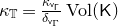 $\kappa _{\mathbb{T}}= \tfrac {\kappa _{\mathsf{v_{\Gamma} }}}{\delta _{{\mathsf v}_{\Gamma} }}\operatorname {Vol}(\mathsf{K})$
.
$\kappa _{\mathbb{T}}= \tfrac {\kappa _{\mathsf{v_{\Gamma} }}}{\delta _{{\mathsf v}_{\Gamma} }}\operatorname {Vol}(\mathsf{K})$
.
5. Proofs of joint equidistribution theorems
This section is devoted to proving Theorems4.4 and 4.5. We keep the notations for ${\mathbb{T}}={\mathbb{T}}({\mathsf v}, \mathsf K), b$
, etc. from Section 4. To simplify notation, we write the proof for the case that
${\mathbb{T}}={\mathbb{T}}({\mathsf v}, \mathsf K), b$
, etc. from Section 4. To simplify notation, we write the proof for the case that $M=M_{\Gamma}$
(e.g.,
$M=M_{\Gamma}$
(e.g., $M$
is connected). The case when
$M$
is connected). The case when $M\ne M_{\Gamma}$
is complicated by the fact that the BMS measure
$M\ne M_{\Gamma}$
is complicated by the fact that the BMS measure $\mathsf m_{\mathsf v}$
on
$\mathsf m_{\mathsf v}$
on $\Gamma \backslash G/M$
has more than one
$\Gamma \backslash G/M$
has more than one $A$
-ergodic component, more precisely, the number of its ergodic components is equal to
$A$
-ergodic component, more precisely, the number of its ergodic components is equal to $[M:M_{\Gamma} ]$
[Reference Lee and OhLO24b], but this can be handled in exactly the same way as in [Reference Chow and FrommCF23, Section 5].
$[M:M_{\Gamma} ]$
[Reference Lee and OhLO24b], but this can be handled in exactly the same way as in [Reference Chow and FrommCF23, Section 5].
Counting in
$\check {N}AMN$
-coordinates

Let $\nu$
and
$\nu$
and $\nu _{{\operatorname {i}}}$
denote the unique
$\nu _{{\operatorname {i}}}$
denote the unique $(\Gamma , \psi _{{\mathsf v}})$
- and
$(\Gamma , \psi _{{\mathsf v}})$
- and $(\Gamma ,\psi _{{\operatorname {i}}({\mathsf v})})$
-conformal measures on
$(\Gamma ,\psi _{{\operatorname {i}}({\mathsf v})})$
-conformal measures on $\mathcal F$
respectively. Let
$\mathcal F$
respectively. Let $\operatorname {Vol}_M$
denote the Haar probability measure on
$\operatorname {Vol}_M$
denote the Haar probability measure on $M$
. Fix bounded Borel sets
$M$
. Fix bounded Borel sets
 \begin{align*} \check {\Xi } \subset \check {N},\;\; \Xi \subset N,\;\; \Theta \subset M\end{align*}
with non-empty relative interiors and null boundaries:
 \begin{align*} \nu (\partial \check {\Xi } e^+)=\nu _{\mathsf{i}}(\partial \Xi ^{-1}e^-)=\operatorname {Vol}_M(\partial \Theta )=0.\end{align*}
For $T \gt 0$
, consider the following subset of
$T \gt 0$
, consider the following subset of $\check {N}A^+MN$
:
$\check {N}A^+MN$
:
 \begin{align} S_{T,b}=S_{T,b}(\check {\Xi },\Xi ,{\mathbb{T}},\Theta ) = \check {\Xi }\exp ({\mathbb{T}}_{T,b}) \Theta \Xi . \end{align}
Define the measures $\tilde {\nu }$
on
$\tilde {\nu }$
on $\check {N}$
and
$\check {N}$
and $\tilde {\nu }_{\mathsf{i}}$
on
$\tilde {\nu }_{\mathsf{i}}$
on $N$
by
$N$
by
 \begin{align*} d\tilde {\nu }(h) = e^{\psi _{\mathsf v}(\beta _{h^+}(e,h))} \, d\nu (h^+) ; \quad d\tilde {\nu }_{\mathsf{i}}(n) = e^{(\psi _{\mathsf v}\circ \mathsf{i})(\beta _{n^-}(e,n))}\, d\nu _{\mathsf{i}}(n^-). \end{align*}
In this subsection, we prove an asymptotic for $\# \Gamma \cap S_{T,b}$
.
$\# \Gamma \cap S_{T,b}$
.
Proposition 5.1.
We have, as $T\to \infty$
,
$T\to \infty$
,
 \begin{align} \#(\Gamma \cap S_{T,b}) \sim c({\mathsf v}, b) \tilde {\nu }(\check {\Xi })\tilde {\nu }_{\mathsf{i}}(\Xi ^{-1})\operatorname {Vol}_M(\Theta )\frac {e^{\delta _{\mathsf v} T}}{T^{({r}-1)/2}} . \end{align}
For a sufficiently small ${\varepsilon }\gt 0$
, consider the following
${\varepsilon }\gt 0$
, consider the following $\varepsilon$
-approximations of
$\varepsilon$
-approximations of $S_{T,b}$
:
$S_{T,b}$
:
 \begin{align*} S_{T,b,\varepsilon }^- = \bigcap _{g_1,g_2 \in G_\varepsilon }g_1S_{T,b}g_2; \quad S_{T,b,\varepsilon }^+ = \bigcup _{g_1,g_2 \in G_\varepsilon }g_1S_{T,b}g_2. \end{align*}
In the next lemma, we state a property of the $\check {N}AMN$
-coordinates that we will use to prove Lemma5.2 which bounds the sets
$\check {N}AMN$
-coordinates that we will use to prove Lemma5.2 which bounds the sets $S_{T,b,\varepsilon }^\pm$
by product subsets of
$S_{T,b,\varepsilon }^\pm$
by product subsets of $\check {N}A^+MN$
that approximate
$\check {N}A^+MN$
that approximate $S_{T,b}$
.
$S_{T,b}$
.
Lemma 5.2.
For all sufficiently small $\varepsilon \gt 0$
, there exist truncated tubes
$\varepsilon \gt 0$
, there exist truncated tubes ${\mathbb{T}}_{T,{\varepsilon }}^{-}\subset {\mathbb{T}}_{T, b}\subset {\mathbb{T}}_{T,{\varepsilon }}^{+}$
and Borel subsets
${\mathbb{T}}_{T,{\varepsilon }}^{-}\subset {\mathbb{T}}_{T, b}\subset {\mathbb{T}}_{T,{\varepsilon }}^{+}$
and Borel subsets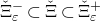 $\check {\Xi }_{\varepsilon }^- \subset \check {\Xi } \subset \check {\Xi }_{\varepsilon }^+$
of
$\check {\Xi }_{\varepsilon }^- \subset \check {\Xi } \subset \check {\Xi }_{\varepsilon }^+$
of $\check N$
,
$\check N$
, $\Xi _{\varepsilon } ^- \subset \Xi \subset \Xi _{\varepsilon } ^+$
of
$\Xi _{\varepsilon } ^- \subset \Xi \subset \Xi _{\varepsilon } ^+$
of $N$
and
$N$
and $\Theta _{\varepsilon }^- \subset \Theta \subset \Theta _{\varepsilon }^+$
of
$\Theta _{\varepsilon }^- \subset \Theta \subset \Theta _{\varepsilon }^+$
of $M$
satisfying the following:
$M$
satisfying the following:
-
1. for all
$T\gt 0$
,(5.3)
\begin{align} \check N_{O(\varepsilon )}\check {\Xi }_{\varepsilon }^- \exp ({\mathbb{T}}_{T,\varepsilon }^-) M_{O(\varepsilon )} \Theta ^-_{\varepsilon } \Xi _{\varepsilon } ^-N_{O(\varepsilon )}\subset S_{T,b,\varepsilon }^- \nonumber \\[5pt] \subset S_{T,b,\varepsilon }^+ \subset \check N_{O(\varepsilon )}\check {\Xi }_{\varepsilon }^+ \exp ({\mathbb{T}}_{T,\varepsilon }^+) M_{O(\varepsilon )} \Theta ^+_{\varepsilon } \Xi _{\varepsilon } ^+N_{O(\varepsilon )} \end{align}
-
2. an
$O(\varepsilon )$
-neighborhood of
${\mathbb{T}}_{T,\varepsilon }^-$
(respectively
${\mathbb{T}}_{T, b}$
) contains
${\mathbb{T}}_{T,b}$
(respectively
${\mathbb{T}}_{T,\varepsilon }^+$
);
-
3.
$\nu ((\check {\Xi }_{\varepsilon }^+ -\check {\Xi }_{\varepsilon }^-) e^+ ) \to 0$
,
$\nu _{\mathsf{i}}((\Xi _{\varepsilon } ^+ -\Xi _{\varepsilon } ^-) e^- ) \to 0$
and
$\operatorname {Vol}_M(\Theta _\varepsilon ^+ - \Theta _{\varepsilon }^-) \to 0$
as
$\varepsilon \to 0$
.






Proof. We prove the half of the lemma involving $-$
signs; the second half involving the
$-$
signs; the second half involving the $+$
signs is similar.
$+$
signs is similar.
For $T\gt 0$
, let
$T\gt 0$
, let ${\mathbb{T}}_{T,\varepsilon }^-$
(respectively
${\mathbb{T}}_{T,\varepsilon }^-$
(respectively $\check {\Xi }_{\varepsilon }^-,\Xi _{\varepsilon } ^-,\Theta _{\varepsilon }^-$
) be the intersection of
$\check {\Xi }_{\varepsilon }^-,\Xi _{\varepsilon } ^-,\Theta _{\varepsilon }^-$
) be the intersection of ${\mathbb{T}}_{T,b}$
(respectively
${\mathbb{T}}_{T,b}$
(respectively $\check {\Xi }_{\varepsilon },\Xi _{\varepsilon } ,\Theta _{\varepsilon }$
) and the complement of an
$\check {\Xi }_{\varepsilon },\Xi _{\varepsilon } ,\Theta _{\varepsilon }$
) and the complement of an $O(\varepsilon )$
-neighborhood of its exterior, or more explicitly,
$O(\varepsilon )$
-neighborhood of its exterior, or more explicitly,
 \begin{align*} {\mathbb{T}}_{T,\varepsilon }^- = {\mathbb{T}}_{T,b} - (\partial {\mathbb{T}}_{T,b}+\mathfrak{a}_{O(\varepsilon )}).\end{align*}
To check (1), let $g\in \check N_{O(\varepsilon )}\check {\Xi }_{\varepsilon }^- \exp ({\mathbb{T}}_{T,\varepsilon }^-) M_{O(\varepsilon )} \Theta ^-_{\varepsilon } \Xi _{\varepsilon }^-N_{O(\varepsilon )}$
. By Lemma2.2(3), it follows that for all
$g\in \check N_{O(\varepsilon )}\check {\Xi }_{\varepsilon }^- \exp ({\mathbb{T}}_{T,\varepsilon }^-) M_{O(\varepsilon )} \Theta ^-_{\varepsilon } \Xi _{\varepsilon }^-N_{O(\varepsilon )}$
. By Lemma2.2(3), it follows that for all $g_1,g_2 \in G_\varepsilon$
,
$g_1,g_2 \in G_\varepsilon$
,
 \begin{align*} g_1^{-1}gg_2^{-1} \in \check N_{O(\varepsilon )}\check {\Xi }_{\varepsilon }^- A_{O(\varepsilon )}\exp ({\mathbb{T}}_{T,\varepsilon }^-) M_{O(\varepsilon )} \Theta ^-_{\varepsilon } \Xi _{\varepsilon }^-N_{O(\varepsilon )} \subset S_{T,b}.\end{align*}
This implies that $g \in S_{T,b,\varepsilon }^-$
, which establishes (1). It is clear that (2) is satisfied. Moreover, since
$g \in S_{T,b,\varepsilon }^-$
, which establishes (1). It is clear that (2) is satisfied. Moreover, since $\nu (\partial \check {\Xi }e^+) = 0$
, we have
$\nu (\partial \check {\Xi }e^+) = 0$
, we have
 \begin{align*} |\nu (\check {\Xi } e^+) - \nu (\check {\Xi }_{\varepsilon }^-e^+)| \le \nu (\check {N}_{O(\varepsilon )}\partial \check {\Xi }e^+) \xrightarrow {\varepsilon \to 0} 0.\end{align*}
Similarly for $\Xi _{\varepsilon } ^-$
and
$\Xi _{\varepsilon } ^-$
and $\Theta _{\varepsilon }^-$
and hence (3) is satisfied.
$\Theta _{\varepsilon }^-$
and hence (3) is satisfied.
An integral over tubes
It is possible to generalize Lemma5.2 by replacing the truncated tubes ${\mathbb{T}}_{T,b}$
with a sequence of sufficiently nice compact subsets of
${\mathbb{T}}_{T,b}$
with a sequence of sufficiently nice compact subsets of $\mathfrak{a}$
and then attempt to obtain the counting as in Proposition5.1 following the well-known approaches of [Reference Eskin and McMullenEM93, Reference Oh and ShahOS13, Reference Mohammadi and OhMO15], etc. However, in carrying out this in this higher rank and infinite volume setting, putting
$\mathfrak{a}$
and then attempt to obtain the counting as in Proposition5.1 following the well-known approaches of [Reference Eskin and McMullenEM93, Reference Oh and ShahOS13, Reference Mohammadi and OhMO15], etc. However, in carrying out this in this higher rank and infinite volume setting, putting
 \begin{align} L({\mathbb{T}}_0)=\frac {\kappa _{\mathsf{v}}}{|m_{\mathcal{X}_{\mathsf v}}|}\int _{t\mathsf{v}+\sqrt {t}u \in {\mathbb{T}}_{0}}e^{\delta _{\mathsf v} t}e^{-I(u)} \, dt \, du \end{align}
where $\kappa _{\mathsf v}$
and
$\kappa _{\mathsf v}$
and $I(u)$
are as in Theorem3.3, we need to control the asymptotic of
$I(u)$
are as in Theorem3.3, we need to control the asymptotic of $L({\mathbb{T}}_{T,b})$
and
$L({\mathbb{T}}_{T,b})$
and $L ({\mathbb{T}}_{T,\varepsilon }^\pm )$
as
$L ({\mathbb{T}}_{T,\varepsilon }^\pm )$
as $T\to \infty$
as in Lemma5.4 where the shape of the tubes plays an important role. We will need the following technical lemma in the proof of Lemma5.4.
$T\to \infty$
as in Lemma5.4 where the shape of the tubes plays an important role. We will need the following technical lemma in the proof of Lemma5.4.
Lemma 5.3.
Define $f_T:\ker \psi _{\mathsf v} \to \mathbb R$
by
$f_T:\ker \psi _{\mathsf v} \to \mathbb R$
by

where $R_T(u) = \{t\ge 0 : t \le T+b(\sqrt {t}u), \sqrt {t}u \in \mathsf{K} \}$
. We have
$R_T(u) = \{t\ge 0 : t \le T+b(\sqrt {t}u), \sqrt {t}u \in \mathsf{K} \}$
. We have
 \begin{align} \lim _{T\to \infty }f_T(u)= \left\{\begin{array}{ll} \frac {1}{\delta _{\mathsf v}}e^{\delta _{\mathsf v} b(u)} & \textrm{if $u\in{\text{int}}\,\mathsf{K}$} \\[5pt] 0 & \textrm{if $u\in\ker\psi_{\mathsf{v}}-\mathsf{K}$} . \end{array}\right.\end{align}
Proof. To compute the desired limit, we will first describe the values in $R_T(u)$
. For convenience, let
$R_T(u)$
. For convenience, let
 \begin{align*} & M_b=\max b; \qquad m_b=\min b; \\[5pt] & J_{u}= \{s\ge 0 : su \in \mathsf{K}\} \quad \textrm{and} \quad J_{u}^2 = \{s^2: s \in J_{u}\} \quad \textrm{for } u\in \ker \psi _{\mathsf v}. \end{align*}
Then
 \begin{align*} \begin{aligned} R_T(u/\sqrt {T}) & = \{t \ge 0: t \le T+b(\sqrt {\tfrac {t}T}u), \, \sqrt {\tfrac {t}T}u \in \mathsf{K}\} \\[5pt] & = \{t\ge 0: t \le T+b(\sqrt {\tfrac {t}T}u), \, t \in T J_{u}^2\} \\[5pt] & \subset \left [0,\min \left \{T+M_b, \left (\sup J_{u}^2\right )T\right \}\right ] \end{aligned} \end{align*}
First, fix $u \in \textrm {int} \mathsf{K}$
. Then
$u \in \textrm {int} \mathsf{K}$
. Then
 \begin{align*} s_u:= \sup \{0\le s\le 1: s u \notin \mathsf K\}\lt 1.\end{align*}
Assume that $T$
is sufficiently large so that
$T$
is sufficiently large so that
 \begin{align*} s_u T \lt T+m_b\lt T+M_b\lt \left (\sup J_{u}^2\right )T.\end{align*}
Observe that $[ s_u T , T+m_b] \subset R_T(u/\sqrt {T})$
and
$[ s_u T , T+m_b] \subset R_T(u/\sqrt {T})$
and $R_T(u/\sqrt {T}) \cap (T+M_b, \infty ) = \emptyset .$
Note that since
$R_T(u/\sqrt {T}) \cap (T+M_b, \infty ) = \emptyset .$
Note that since $s_u \lt 1$
, we have
$s_u \lt 1$
, we have
 \begin{align} \frac {1}{e^{\delta _{\mathsf v} T}}e^{- I(u)/T} \int _0^{s_uT} e^{\delta _{\mathsf v} t}\, dt \le \frac {1}{e^{\delta _{\mathsf v} T}}e^{- I(u)/T} e^{\delta _{\mathsf v} s_uT} \end{align}
and hence the quantity on the left-hand side goes to $0$
as
$0$
as $T \to \infty$
.
$T \to \infty$
.
Next we investigate which values in $[T+m_b, T+M_b]$
are in
$[T+m_b, T+M_b]$
are in $R_T(u/\sqrt {T})$
. Fix
$R_T(u/\sqrt {T})$
. Fix $\varepsilon \gt 0$
. Using continuity of
$\varepsilon \gt 0$
. Using continuity of $b$
, we note that for all
$b$
, we note that for all $T$
sufficiently large and for all
$T$
sufficiently large and for all $\eta \in (\varepsilon , b(u) - m_b)$
, we have
$\eta \in (\varepsilon , b(u) - m_b)$
, we have
 \begin{align*} T+b(u)-\eta \lt T+b\left (\sqrt {\tfrac {T+b(u)-\eta }T}u\right )\end{align*}
and henceFootnote 6
 \begin{align} [s_u T , T+b(u) - o_T(1)] \subset R_T(u/\sqrt {T}). \end{align}
Similarly, we note that for all $T$
sufficiently large and for all
$T$
sufficiently large and for all $\eta \in (\varepsilon , M_b - b(u))$
, we have
$\eta \in (\varepsilon , M_b - b(u))$
, we have
 \begin{align*} T+b(u)+\eta \gt T+b\left (\sqrt {\tfrac {T+b(u)+\eta }T}u\right )\end{align*}
and hence
 \begin{align} R_T(u/\sqrt {T})\cap [T+b(u)+o_T(1) , \infty ) = \emptyset . \end{align}
Also note that
 \begin{align} \frac {e^{- I(u)/T}}{e^{\delta _{\mathsf v} T}} \int _{T+b(u)-o_T(1)}^{T+b(u)+o_T(1)} e^{\delta _{\mathsf v} t}\, dt = \frac {1}{e^{\delta _{\mathsf v} T}}e^{- I(u)/T} e^{\delta _{\mathsf v} b(u)}(e^{o_T(1)}-e^{-o_T(1)}) \end{align}
goes to $0$
as
$0$
as $T \to \infty$
. Summarizing (5.6)–(5.9), we have shown that to compute
$T \to \infty$
. Summarizing (5.6)–(5.9), we have shown that to compute $\lim _{T\to \infty }f_T(u)$
, we can replace
$\lim _{T\to \infty }f_T(u)$
, we can replace $R_T(u/\sqrt {T})$
with
$R_T(u/\sqrt {T})$
with $[s_T, T+b(u)-o_T(1)]$
to get
$[s_T, T+b(u)-o_T(1)]$
to get
 \begin{align*} \lim _{T\to \infty }f_T(u) & = \lim _{T\to \infty }\frac {1}{e^{\delta _{\mathsf v} T}}e^{- I(u)/T} \int _{R_T(u/\sqrt {T})} e^{\delta _{\mathsf v} t}\, dt \\[5pt] & = \lim _{T\to \infty }\frac {1}{\delta _{\mathsf v} e^{\delta _{\mathsf v} T}}e^{- I(u)/T} (e^{\delta _{\mathsf v}(T+b(u)-o_T(1))} - o_T(e^{\delta _{\mathsf v} T})) \\[5pt] & = \frac {1}{\delta _{\mathsf v}}e^{\delta _{\mathsf v} b(u)}. \end{align*}
Next, fix $u \notin \mathsf{K}$
. Since
$u \notin \mathsf{K}$
. Since $\mathsf{K}$
is closed, there exists
$\mathsf{K}$
is closed, there exists $\eta \gt 0$
such that
$\eta \gt 0$
such that $(1-\eta ,1+\eta )\cap J_u = \emptyset$
. Then for all sufficiently large
$(1-\eta ,1+\eta )\cap J_u = \emptyset$
. Then for all sufficiently large $T$
, we have
$T$
, we have
 \begin{align*} R_T(u/\sqrt {T}) = \Big\{t\ge 0: t \le T+b\Big(\sqrt {\tfrac {t}T}u\Big), \, t \in T J_{u}^2\Big\} \subset [0,(1-\eta )^2T]. \end{align*}
Then
 \begin{align*} f_T(u) \le \frac {1}{e^{\delta _{\mathsf v} T}}e^{- I(u)/T} \int _0^{(1-\eta )^2T} e^{\delta _{\mathsf v} t}\, dt \le \frac {1}{e^{\delta _{\mathsf v} T}}e^{- I(u)/T} e^{\delta _{\mathsf v} (1-\eta )^2T}\end{align*}
and hence $\lim _{T\to \infty }f_T(u)=0$
.
$\lim _{T\to \infty }f_T(u)=0$
.
Lemma 5.4. We have
 \begin{align} \lim \limits _{T\to \infty }\frac {1}{e^{\delta _{\mathsf v} T} T^{(1-{r})/2}}\int _{t\mathsf{v}+\sqrt {t}u \in {\mathbb{T}}_{T,b}}e^{\delta _{\mathsf v} t} e^{- I(u)} \, dt \, du =\frac {1}{\delta _{\mathsf v}}\int _{\mathsf{K}} e^{\delta _{\mathsf v} b(u)} \, du. \end{align}
Proof. We may assume ${\mathbb{T}}_{T,b} = \{t{\mathsf v}+u:0\le t\le T+b(u), \, u \in \mathsf{K}\}$
as
${\mathbb{T}}_{T,b} = \{t{\mathsf v}+u:0\le t\le T+b(u), \, u \in \mathsf{K}\}$
as ${\mathbb{T}}_{T,b}- \mathfrak{a}^+$
is contained in a fixed compact set independent of
${\mathbb{T}}_{T,b}- \mathfrak{a}^+$
is contained in a fixed compact set independent of $T$
. Then
$T$
. Then
 \begin{align*} R_T(u) = \{t\ge 0 : t \le T+b(\sqrt {t}u), \sqrt {t}u \in \mathsf{K} \}.\end{align*}
By changing the variable $\sqrt {T}u$
to
$\sqrt {T}u$
to $u$
, we have
$u$
, we have
 \begin{align*} \begin{aligned}[b] & \frac {1}{ e^{\delta _{\mathsf v} T}T^{(1-{r})/2}}\int _{t\mathsf{v}+\sqrt {t}u \in {\mathbb{T}}_{T,b}}e^{\delta _{\mathsf v} t} e^{- I(u)} \, dt \, du \\[5pt] & = \frac {1}{ e^{\delta _{\mathsf v} T}T^{(1-{r})/2}}\int _{\ker \psi _{\mathsf v}}e^{- I(u)} \int _{R_T(u)} e^{\delta _{\mathsf v} t}\, dt \, du \\[5pt] & = \int _{\ker \psi _{\mathsf v}}\frac {1}{e^{\delta _{\mathsf v} T}}e^{- I(u)/T} \int _{R_T(u/\sqrt {T})} e^{\delta _{\mathsf v} t}\, dt \, du\\[5pt] & =\int _{\ker \psi _{\mathsf v}} f_T. \end{aligned} \end{align*}
Set
 \begin{align*} \mathsf A_T= \int _{u \in \textrm {int} \mathsf{K}} f_T, \;\; \mathsf B_T= \int _{u\in \textrm{hull} (\mathsf{K}\cup \{0\}) -\mathsf K} f_T \quad \textrm{and}\quad \mathsf C_T= \int _{u\notin \textrm{hull}(\mathsf{K} \cup \{0\})} f_T \end{align*}
where $\textrm{hull}\mathsf K\cup \{0\}$
means the convex hull of
$\textrm{hull}\mathsf K\cup \{0\}$
means the convex hull of $\mathsf K \cup \{0\}$
. By hypothesis that
$\mathsf K \cup \{0\}$
. By hypothesis that $\partial \mathsf K$
has measure zero, we have
$\partial \mathsf K$
has measure zero, we have $\int _{\ker \psi _{\mathsf v}} f_T= \mathsf A_T + \mathsf B_T + \mathsf C_T$
.
$\int _{\ker \psi _{\mathsf v}} f_T= \mathsf A_T + \mathsf B_T + \mathsf C_T$
.
We obtain the asymptotics of $\mathsf A_T$
,
$\mathsf A_T$
, $\mathsf B_T$
and
$\mathsf B_T$
and $\mathsf C_T$
below.
$\mathsf C_T$
below.
2.1. Asymptotic of
$\mathsf A_T$

Since
 \begin{align*} \begin{aligned} R_T(u/\sqrt {T}) & = \Big\{t \ge 0: t \le T+b\Big(\sqrt {\tfrac {t}T}u\Big), \, \sqrt {\tfrac {t}T}u \in \mathsf{K}\Big\} \\ & = \Big\{t\ge 0: t \le T+b\Big(\sqrt {\tfrac {t}T}u\Big), \, t \in T J_{u}^2\Big\} \\ & \subset \left [0,\min \left \{T+M_b, \left (\sup J_{u}^2\right )T\right \}\right ]\\[12pt] \end{aligned} \end{align*}
where $J_{u}= \{s\ge 0 : su \in \mathsf{K}\}$
, we have for all
$J_{u}= \{s\ge 0 : su \in \mathsf{K}\}$
, we have for all $u \in \ker \psi _{\mathsf v}$
,
$u \in \ker \psi _{\mathsf v}$
,
 \begin{align*} f_T(u) \le \frac {1}{e^{\delta _{\mathsf v} T}} \int _0^{T+M_b} e^{\delta _{\mathsf v} t}\, dt \le \frac {1}{\delta _{\mathsf v}}e^{\delta _{\mathsf v} M_b}. \end{align*}
Since $\mathsf K$
is bounded and the integral in (5) is uniformly bounded for all
$\mathsf K$
is bounded and the integral in (5) is uniformly bounded for all $T$
we can apply the Lebesgue dominated convergence theorem for the sequence
$T$
we can apply the Lebesgue dominated convergence theorem for the sequence $f_T|_{\operatorname {int} \mathsf K}$
to compute the asymptotic of
$f_T|_{\operatorname {int} \mathsf K}$
to compute the asymptotic of $\mathsf A_T$
using Lemma5.3:
$\mathsf A_T$
using Lemma5.3:
 \begin{align*} \lim _{T\to \infty } {\mathsf A_T}= \int _{u \in \textrm {int} \mathsf{K}} \lim _{T\to \infty }f_T( u) du = \frac {1}{\delta _{\mathsf v}}\int _{u \in \textrm {int} \mathsf{K}}e^{\delta _{\mathsf v} b(u)} \, du. \end{align*}
Hence it suffices to show that $\mathsf B_T+\mathsf C_T$
converges to
$\mathsf B_T+\mathsf C_T$
converges to $0$
as
$0$
as $T\to \infty$
.
$T\to \infty$
.
Asymptotic of
$\mathsf B_T$

For $u\in\textrm{hull} (\mathsf{K} \cup \{0\})$
, we still have the constant upper bound in (5). Hence we can also apply the Lebesgue dominated convergence theorem and Lemma5.3 to compute
$u\in\textrm{hull} (\mathsf{K} \cup \{0\})$
, we still have the constant upper bound in (5). Hence we can also apply the Lebesgue dominated convergence theorem and Lemma5.3 to compute
 \begin{align*} \lim _{T\to \infty } \mathsf{B}_T = \int _{u\in \textrm{hull} (\mathsf{K}\cup \{0\}) -\mathsf K}\lim _{T\to \infty }f_T(u) \, du = \int _{u\in \textrm{hull} (\mathsf{K}\cup \{0\}) -\mathsf K}0 \, du=0 \end{align*}
Asymptotic of
$\mathsf C_T$

Fix $u\notin \textrm{hull}(\mathsf K\cup \{0\})$
. Then for all
$u\notin \textrm{hull}(\mathsf K\cup \{0\})$
. Then for all $t \ge 1$
,
$t \ge 1$
, $tu\notin \mathsf{K}$
otherwise
$tu\notin \mathsf{K}$
otherwise $u$
would lie on the segment with endpoints
$u$
would lie on the segment with endpoints $0$
and
$0$
and $tu$
and be in
$tu$
and be in $\textrm{hull}(\mathsf{K} \cup \{0\})$
. In particular, we have
$\textrm{hull}(\mathsf{K} \cup \{0\})$
. In particular, we have
 \begin{align*} j_{u}: = \sup ( J_{u})= \sup \{0\le s\le 1 : su \in \mathsf{K}\} \lt 1. \end{align*}
Define
 \begin{align*} g(u):={ 2\sqrt {\delta _{\mathsf v} I(u)(1-j_{u}^2)}} .\end{align*}
Using $R_T(u/\sqrt {T}) \subset TJ_{u}^2 \subset T[0,j_{u}^2]$
, we get for all
$R_T(u/\sqrt {T}) \subset TJ_{u}^2 \subset T[0,j_{u}^2]$
, we get for all $T\gt 0$
,
$T\gt 0$
,
 \begin{align*} f_T(u) =\frac {1}{e^{\delta _{\mathsf v} T}}e^{- I(u)/T} \int _{R_T(u/\sqrt {T})} e^{\delta _{\mathsf v} t}\, dt \le \tfrac {1}{\delta _{\mathsf v}}e^{- I(u)/T}e^{-\delta _{\mathsf v} T(1-j_{u}^2)} \le \tfrac {1}{\delta _{\mathsf v}}e^{- g(u)}, \end{align*}
where the last inequality uses the fact that $a+b \ge 2\sqrt {ab}$
for all
$a+b \ge 2\sqrt {ab}$
for all $a,b \ge 0$
. Note that the function
$a,b \ge 0$
. Note that the function $g(u)$
is radially increasing with at least a linear rate: for all
$g(u)$
is radially increasing with at least a linear rate: for all $r\gt 1$
, we have
$r\gt 1$
, we have
 \begin{align*} g(ru)={2 \sqrt {\delta _{\mathsf v} I(r u)(1-j_{r u}^2)}} =2r\sqrt {\delta _{\mathsf v} I(u)(1-j_{u}^2/r^2)} \ge r g(u),\end{align*}
so the function $u\mapsto e^{-g(u)}$
is
$u\mapsto e^{-g(u)}$
is $L^1$
-integrable on
$L^1$
-integrable on $\ker \psi _{\mathsf v} -\textrm{hull}(\mathsf{K} \cup \{0\})$
. Hence we apply the Lebesgue dominated convergence theorem to compute the asymptotic of
$\ker \psi _{\mathsf v} -\textrm{hull}(\mathsf{K} \cup \{0\})$
. Hence we apply the Lebesgue dominated convergence theorem to compute the asymptotic of $\mathsf C_T$
using Lemma5.3:
$\mathsf C_T$
using Lemma5.3:
 \begin{align*} \lim _{T\to \infty } \mathsf{C}_T = \int _{u\notin \textrm{hull} (\mathsf{K}\cup \{0\})}\lim _{T\to \infty }f_T(u) \, du = \int _{u\notin \textrm{hull} (\mathsf{K}\cup \{0\})}0 \, du=0. \end{align*}
This finishes the proof of Lemma5.4.
We are now ready to give the proof of Proposition5.1.
Proof of Proposition5.1
We first introduce some notation. Given a bounded Borel subset $B$
of
$B$
of $G$
, define the counting function
$G$
, define the counting function $F_B: G \times G \to \mathbb N$
by
$F_B: G \times G \to \mathbb N$
by
 \begin{align*} F_B(g,h) = \sum _{\gamma \in \Gamma } 1_B(g^{-1}\gamma h).\end{align*}
Note that $ F_{S_{T,b}}(e,e) = \#\Gamma \cap S_{T,b}$
. The function
$ F_{S_{T,b}}(e,e) = \#\Gamma \cap S_{T,b}$
. The function $F_B$
is
$F_B$
is $\Gamma$
-invariant in both arguments so it descends to a function on
$\Gamma$
-invariant in both arguments so it descends to a function on $\Gamma \backslash G \times \Gamma \backslash G$
which we still denote by
$\Gamma \backslash G \times \Gamma \backslash G$
which we still denote by $F_B$
. For
$F_B$
. For $F_1,F_2 :\Gamma \backslash G \times \Gamma \backslash G \to {\mathbb R}$
, let
$F_1,F_2 :\Gamma \backslash G \times \Gamma \backslash G \to {\mathbb R}$
, let
 \begin{align*} \langle F_1,F_2 \rangle = \int _{\Gamma \backslash G \times \Gamma \backslash G}F_1(x_1,x_2)F_2(x_1,x_2) \, dx_1 \, dx_2\end{align*}
when the integral makes sense where $dx_1,dx_2$
are both the Haar measure on
$dx_1,dx_2$
are both the Haar measure on $\Gamma \backslash G$
. For
$\Gamma \backslash G$
. For $\varepsilon \gt 0$
smaller than the injectivity radius of
$\varepsilon \gt 0$
smaller than the injectivity radius of $\Gamma$
at
$\Gamma$
at $e$
, we fix a nonnegative function
$e$
, we fix a nonnegative function $\psi _\varepsilon \in C^\infty (G)$
with
$\psi _\varepsilon \in C^\infty (G)$
with $\operatorname {supp} \psi _\varepsilon \subset G_\varepsilon$
and
$\operatorname {supp} \psi _\varepsilon \subset G_\varepsilon$
and $\int _G \psi _\varepsilon \, dg=1$
. Let
$\int _G \psi _\varepsilon \, dg=1$
. Let $\Psi _\varepsilon \in C^\infty (\Gamma \backslash G)$
be defined by
$\Psi _\varepsilon \in C^\infty (\Gamma \backslash G)$
be defined by $\Psi _\varepsilon (\Gamma g) = \sum _{\gamma \in \Gamma } \psi _\varepsilon (\gamma g)$
for all
$\Psi _\varepsilon (\Gamma g) = \sum _{\gamma \in \Gamma } \psi _\varepsilon (\gamma g)$
for all $g \in G$
.
$g \in G$
.
Observe that we have
 \begin{align} \langle F_{S_{T,b,\varepsilon }^-}, \Psi _\varepsilon \otimes \Psi _\varepsilon \rangle \le F_{S_{T,b}}(e,e) \le \langle F_{S_{T,b,\varepsilon }^+}, \Psi _\varepsilon \otimes \Psi _\varepsilon \rangle . \end{align}
Given a bounded Borel subset $B \subset G$
, we define
$B \subset G$
, we define $f_{B}:\check {N}\times MN \to {\mathbb R}$
by
$f_{B}:\check {N}\times MN \to {\mathbb R}$
by
 \begin{align*} f_{B}(h,mn) = \tfrac {\kappa _{\mathsf{v}}}{|m_{\mathcal{X}_{\mathsf v}}|}\int _{h^{-1}a_{t\mathsf{v}+\sqrt {t}u}mn \in B}e^{\delta _{\mathsf v} t}e^{-I(u)} \, dt \, du. \end{align*}
Continuing the notation (5.4), set
 \begin{align*} L({\mathbb{T}}_{T,b})=\tfrac {\kappa _{\mathsf{v}}}{|m_{\mathcal{X}_{\mathsf v}}|}\int _{t\mathsf{v}+\sqrt {t}u \in {\mathbb{T}}_{T,b}}e^{\delta _{\mathsf v} t}e^{-I(u)} \, dt \, du\end{align*}
which is the value of $f_{S_{T,b}}(h,mn)$
when it is non-zero.
$f_{S_{T,b}}(h,mn)$
when it is non-zero.
We denote by
 \begin{align*} & I_1: MAN\check {N} \to \mathfrak{a}, & J_1: MAN\check {N} \to \check {N}, \\ & I_2: A\check {N}MN \to \mathfrak{a}, & J_2: A\check {N}MN \to MN \end{align*}
the natural projection maps. For a bounded subset $B \subset G$
, define
$B \subset G$
, define
 \begin{align*} \tilde f_{B}(g_1,g_2) = f_{B} {(J_1(g_1^{-1}),J_2(g_2^{-1})) } e^{\psi _{\mathsf v}(I_1(g_1^{-1})-I_2(g_2^{-1}))} \end{align*}
for any $g_i\in G$
such that
$g_i\in G$
such that $J(g_i^{-1})$
and
$J(g_i^{-1})$
and $I(g_i^{-1})$
are defined for
$I(g_i^{-1})$
are defined for $i=1,2$
.
$i=1,2$
.
The first step is to rewrite $\langle F_{S_{T,b,\varepsilon }^\pm }, \Psi _\varepsilon \otimes \Psi _\varepsilon \rangle$
by decomposing the Haar measure on
$\langle F_{S_{T,b,\varepsilon }^\pm }, \Psi _\varepsilon \otimes \Psi _\varepsilon \rangle$
by decomposing the Haar measure on $G$
using
$G$
using $\check {N}AMN$
coordinates and separating the expected main term from local mixing from the error term. Set
$\check {N}AMN$
coordinates and separating the expected main term from local mixing from the error term. Set $Q_{S_{T,b,\varepsilon }^\pm }$
to be
$Q_{S_{T,b,\varepsilon }^\pm }$
to be
 \begin{align} \int _{K/M\times K}\int _{G_\varepsilon \times G_\varepsilon } \tilde f_{S_{T,b,\varepsilon }^\pm }(g_1^{-1} k_1,g_2^{-1} k_2) \cdot \psi _\varepsilon (g_1) \psi _\varepsilon (g_2) \, dg_1 \, dg_2 \, d\nu (k_1^+) \, d\nu _{\mathsf{i}}(k_2^+). \end{align}
Then as in [Reference Chow and FrommCF23, Lemmas 5.4–5.8], we have
 \begin{align*} & \langle F_{S_{T,b,\varepsilon }^\pm }, \Psi _\varepsilon \otimes \Psi _\varepsilon \rangle \\ & = Q_{S_{T,b,\varepsilon }^\pm } +\int _{h^{-1}a_{t\mathsf{v}+\sqrt {t}u}mn \in S_{T,b,\varepsilon }^\pm }e^{\delta _{\mathsf v} t}E_\varepsilon (t,u,h,mn) \, dt \, du \, dh \, dm \, dn \end{align*}
where
 \begin{align*} E_\varepsilon (t,u,h,mn) = t^{({r}-1)/2}e^{2\rho (t\mathsf{v}+\sqrt {t}u)-\delta _{\mathsf v} t}\int _{\Gamma \backslash G} \Psi _\varepsilon (xh)\Psi _\varepsilon (xa_{t\mathsf{v}+\sqrt {t}u}mn) \, dx \\ - \tfrac {\kappa _{\mathsf{v}}e^{-I(u)}}{|m_{\mathcal{X}_{\mathsf v}}|}\mathsf{m}^{\textrm{BR}_\star }_{\mathsf v}\bigr (h^{-1}.\Psi _\varepsilon )\mathsf{m}^{\textrm{BR}}_{\mathsf v}\bigr ((mn)^{-1}.\Psi _\varepsilon ). \end{align*}
In view of (5.12) and Lemma5.2, we only need to consider $k_1 \in K$
such that
$k_1 \in K$
such that $J_1(k_1^{-1}g_1)$
is in a bounded set. Similarly for
$J_1(k_1^{-1}g_1)$
is in a bounded set. Similarly for $k_2$
. Then by Lemma2.2(1)-(2), we get
$k_2$
. Then by Lemma2.2(1)-(2), we get
 \begin{align*} \psi _{\mathsf v}(I_1(k_1^{-1}g_1))=\psi _{\mathsf v}(I_1(k_1^{-1}))+O(\varepsilon ); \quad \psi _{\mathsf v}(I_2(k_2^{-1}g_2))=\psi _{\mathsf v}(I_2(k_2^{-1}))+O(\varepsilon ) \end{align*}
and
 \begin{align} \begin{aligned}[b] & J_1(k_1^{-1}g_1)^{-1} \in \check {N}_{O(\varepsilon )} J_1(k_1^{-1})^{-1}; & J_2(k_2^{-1} g_2) \in M_{O(\varepsilon )}J_2(k_2^{-1})N_{O(\varepsilon )}. \end{aligned} \end{align}
Let ${\mathbb{T}}_{T,\varepsilon }^- = {\mathbb{T}}({\mathsf v},\mathsf{K}_\varepsilon ^-,T,b_\varepsilon ^-) \subset {\mathbb{T}}_{T,b}$
,
${\mathbb{T}}_{T,\varepsilon }^- = {\mathbb{T}}({\mathsf v},\mathsf{K}_\varepsilon ^-,T,b_\varepsilon ^-) \subset {\mathbb{T}}_{T,b}$
, $\check {\Xi }_{\varepsilon }^- \subset \check {\Xi }$
,
$\check {\Xi }_{\varepsilon }^- \subset \check {\Xi }$
, $\Xi _{\varepsilon } ^- \subset \Xi$
and
$\Xi _{\varepsilon } ^- \subset \Xi$
and $\Theta _{\varepsilon }^- \subset \Theta$
be as in Lemma5.2. For convenience, let
$\Theta _{\varepsilon }^- \subset \Theta$
be as in Lemma5.2. For convenience, let
 \begin{align*} S_{T,b_\varepsilon ^-}:=\check {\Xi }_{\varepsilon }^- \exp ({\mathbb{T}}_{T,\varepsilon }^-) \Theta _{\varepsilon }^- \Xi _{\varepsilon } ^-.\end{align*}
By Lemma5.2(1) and (5.13), for all $g_1,g_2\in G_\varepsilon$
we have
$g_1,g_2\in G_\varepsilon$
we have
 \begin{align*} f_{S_{T,b,\varepsilon }^-}(J_1(k_1^{-1}g_1),J_2(k_2^{-1}g_2)) \ge f_{S_{T,b_\varepsilon ^-}}(J_1(k_1^{-1}),J_2(k_2^{-1})).\end{align*}
It now follows that
 \begin{align} Q_{S_{T,b,\varepsilon }^-} \ge \int _{K/M\times K} (1+O(\varepsilon )) \tilde f_{S_{T,b_\varepsilon ^-}}(k_1, k_2) \, d\nu (k_1^+) \, d\nu _{\mathsf{i}}(k_2^+). \end{align}
Using Lemma5.2(2)–(3), we observe thatFootnote 7
 \begin{align} \begin{aligned}[b] & \int _{K/M\times K} (f_{S_{T,b}} - f_{S_{T,b_\varepsilon ^-}})(J_1(k_1^{-1}),J_2(k_2^{-1})) \, d\nu (k_1^+)\, d\nu _{\mathsf{i}}(k_2^+) \\ & =L({\mathbb{T}}_{T,b})O\left (\nu \left ((\check {\Xi }- \check {\Xi }_{\varepsilon }^-)e^+\right ) + \nu _{\mathsf{i}}\left ((\Xi ^{-1}- (\Xi _{\varepsilon } ^-)^{-1})e^- \right ) + \operatorname {Vol}_M\left (\Theta -\Theta _{\varepsilon }^-\right ) \right ) \\ & \qquad \qquad \qquad + (L({\mathbb{T}}_{T,b}) - L({\mathbb{T}}_{T,\varepsilon }^-))\nu (\check {\Xi }_{\varepsilon }^-)\nu ((\Xi _{\varepsilon } ^-)^{-1})\operatorname {Vol}_M(\Theta ^-) \\ & = L({\mathbb{T}}_{T,b})o_\varepsilon (1)+O(L({\mathbb{T}}_{T,b}) - L({\mathbb{T}}_{T,\varepsilon }^-)) \\ & = L({\mathbb{T}}_{T,b})o_\varepsilon (1) \end{aligned} \end{align}
where we note that $L({\mathbb{T}}_{T,b}) - L({\mathbb{T}}_{T,\varepsilon }^-) = L({\mathbb{T}}_{T,b})o_\varepsilon (1)$
by Lemma5.4.Footnote
8
$L({\mathbb{T}}_{T,b}) - L({\mathbb{T}}_{T,\varepsilon }^-) = L({\mathbb{T}}_{T,b})o_\varepsilon (1)$
by Lemma5.4.Footnote
8
Combining (5.14) and (5.15) yields
 \begin{align} Q_{S_{T,b,\varepsilon }^-} \ge \int _{K/M\times K} (1+O(\varepsilon )) \tilde f_{S_{T,b}}(k_1, k_2) d\nu (k_1^+) \, d\nu _{\mathsf{i}}(k_2^+) + L({\mathbb{T}}_{T,b})o_\varepsilon (1). \end{align}
A similar argument shows that
 \begin{align} Q_{S_{T,b,\varepsilon }^+} \le \int _{K/M\times K} (1+O(\varepsilon )) \tilde f_{S_{T,b}}(k_1, k_2) d\nu (k_1^+) \, d\nu _{\mathsf{i}}(k_2^+) + L({\mathbb{T}}_{T,b})o_\varepsilon (1) \end{align}
and we conclude that
 \begin{align} Q_{S_{T,b,\varepsilon }^\pm } = \int _{K/M\times K} (1+O(\varepsilon )) \tilde f_{S_{T,b}} \, d\nu (k_1^+) \, d\nu _{\mathsf{i}}(k_2^+) + L({\mathbb{T}}_{T,b})o_\varepsilon (1). \end{align}
Considering $k_1 \in K$
such that
$k_1 \in K$
such that $k_1^{-1} = ma_wnh^{-1} \in MAN\check {N},$
we have
$k_1^{-1} = ma_wnh^{-1} \in MAN\check {N},$
we have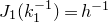 $J_1(k_1^{-1}) = h^{-1}$
,
$J_1(k_1^{-1}) = h^{-1}$
, $h^+ = k_1M$
,
$h^+ = k_1M$
, $I_1(k_1^{-1}) = w = \beta _{h^+}(e,h)$
and hence
$I_1(k_1^{-1}) = w = \beta _{h^+}(e,h)$
and hence
 \begin{align*} \int _{{k_1^+\in K/M ,\, (J_1(k_1^{-1}))^{-1} \in \check {\Xi }}} e^{\psi _{\mathsf v}(I_1(k_1^{-1}))} \, d\nu (k_1^+) = \int _{h \in \check {\Xi }} e^{\psi _{\mathsf v}(\beta _{h^+}(e,h))} \, d\nu (h^+) = \tilde {\nu }(\check {\Xi }). \end{align*}
Similarly, considering $k_2 \in K$
such that
$k_2 \in K$
such that $k_2^{-1} = a_whm^{-1}n^{-1} \in A\check {N}MN,$
we have
$k_2^{-1} = a_whm^{-1}n^{-1} \in A\check {N}MN,$
we have $J_2(k_2^{-1}) = m^{-1}n^{-1} \in MN$
,
$J_2(k_2^{-1}) = m^{-1}n^{-1} \in MN$
, $k_2^- = n^-$
,
$k_2^- = n^-$
, $I_2(k_2^{-1}) =w=-i(\beta _{n^-}(e,n))$
and hence
$I_2(k_2^{-1}) =w=-i(\beta _{n^-}(e,n))$
and hence
 \begin{align*} \int _{{k_2 \in K ,\, J_2(k_2^{-1}) \in \Theta \Xi }} e^{-\psi _{\mathsf v}(I_2(k_2^{-1}))}d\nu _{\mathsf{i}}(k_2^+) & = \int _{nm \in \Xi ^{-1}\Theta ^{-1}}e^{(\psi _{\mathsf v}\circ \mathsf{i})(\beta _{n^-}(e,n))}\, d\nu _{\mathsf{i}}(n^-) \, dm \\ & = \tilde {\nu }_{\mathsf{i}}(\Xi ^{-1})\operatorname {Vol}_M(\Theta ). \end{align*}
Thus, we obtain
 \begin{align*} & \langle F_{S_{T,b,\varepsilon }^\pm }, \Psi _\varepsilon \otimes \Psi _\varepsilon \rangle \\ & = (1+O(\varepsilon ))L({\mathbb{T}}_{T,b})\tilde {\nu }(\check {\Xi })\tilde {\nu }_{\mathsf{i}}(\Xi ^{-1})\operatorname {Vol}_M(\Theta ) \\ & \quad +\int _{h^{-1}a_{t\mathsf{v}+\sqrt {t}u}mn \in S_{T,b,\varepsilon }^\pm }e^{\delta _{\mathsf v} t}E_\varepsilon (t,u,h,mn) \, dt \, du \, dh \, dm \, dn +L({\mathbb{T}}_{T,b})o_\varepsilon (1). \end{align*}
For the error term $E_\varepsilon (t,u,h,mn)$
, we claim that
$E_\varepsilon (t,u,h,mn)$
, we claim that
 \begin{align} \lim \limits _{T\to \infty }\frac {1}{e^{\delta _{\mathsf v} T} T^{(1-{r})/2}}\int _{h^{-1}a_{t\mathsf{v}+\sqrt {t}u}mn \in S_{T,b,\varepsilon }^\pm }e^{\delta _{\mathsf v} t}E_\varepsilon (t,u,h,mn) \, dt \, du \, dh \, dm \, dn=0. \end{align}
To prove (5.19), note that since $\check {\Xi } \subset \check {N}$
and
$\check {\Xi } \subset \check {N}$
and $\Xi \subset N$
are bounded, by Theorem3.3, there exist positive constants
$\Xi \subset N$
are bounded, by Theorem3.3, there exist positive constants $\eta _{\mathsf{v}}, D_{\mathsf{v}}$
and
$\eta _{\mathsf{v}}, D_{\mathsf{v}}$
and $s_{\mathsf{v}}$
such that
$s_{\mathsf{v}}$
such that
 \begin{align*} |E_\varepsilon (t,u,h,mn)| \le D_{\mathsf{v}} e^{-\eta _{\mathsf{v}} I(u)}\end{align*}
for all $(t,u) \in (s_{\mathsf{v}},\infty ) \times \ker \psi _{\mathsf{v}}$
and
$(t,u) \in (s_{\mathsf{v}},\infty ) \times \ker \psi _{\mathsf{v}}$
and $h,mn$
such that
$h,mn$
such that $h^{-1}a_{t\mathsf{v}+\sqrt {t}u}mn \in S_{T,b,\varepsilon }^\pm$
. Then (5.19) follows by using similar reasoning as in Lemma5.4 and the fact that for fixed
$h^{-1}a_{t\mathsf{v}+\sqrt {t}u}mn \in S_{T,b,\varepsilon }^\pm$
. Then (5.19) follows by using similar reasoning as in Lemma5.4 and the fact that for fixed $u \in \ker \psi _{\mathsf v}$
,
$u \in \ker \psi _{\mathsf v}$
, $\lim \limits _{t\to \infty }E_\varepsilon (t,u,h,mn)=0$
.
$\lim \limits _{t\to \infty }E_\varepsilon (t,u,h,mn)=0$
.
Now using Lemma5.4 and (5.11), taking $T\to \infty$
and then
$T\to \infty$
and then $\varepsilon \to 0$
, we conclude that
$\varepsilon \to 0$
, we conclude that
 \begin{align*} \#(\Gamma \cap S_T) \sim \frac {\kappa _{\mathsf{v}}}{\delta _{\mathsf v}|m_{\mathcal{X}_{\mathsf v}}|}\int _{\mathsf{K}} e^{\delta _{\mathsf v} b(u)} \, du \cdot \tilde {\nu }(\check {\Xi })\tilde {\nu }_{\mathsf{i}}(\Xi ^{-1})\operatorname {Vol}_M(\Theta ).\end{align*}
This finishes the proof of Proposition5.1.
Counting via flow boxes
We use flow boxes as in [Reference MargulisMar04] and [Reference Margulis, Mohammadi and OhMMO14].
Definition 5.5 ( $\varepsilon$
-flow box at
$\varepsilon$
-flow box at $g_0$
). Given
$g_0$
). Given $g_0 \in G$
and
$g_0 \in G$
and $\varepsilon \gt 0$
, the
$\varepsilon \gt 0$
, the $\varepsilon$
-
$\varepsilon$
- $g_0$
is defined by
$g_0$
is defined by
 \begin{align*} \mathcal{B}(g_0,\varepsilon )=g_0(\check {N}_\varepsilon N \cap N_\varepsilon \check {N} AM)M_\varepsilon A_\varepsilon .\end{align*}
We denote the projection of $\mathcal{B}(g_0,\varepsilon )$
into
$\mathcal{B}(g_0,\varepsilon )$
into $\Gamma \backslash G/M$
by
$\Gamma \backslash G/M$
by $\tilde {\mathcal{B}}(g_0,\varepsilon )$
.
$\tilde {\mathcal{B}}(g_0,\varepsilon )$
.
For $g_0\in G$
and
$g_0\in G$
and $T, \varepsilon \gt 0$
, we denote
$T, \varepsilon \gt 0$
, we denote
 \begin{align} \mathcal{V}_{T,b}(g_0,\varepsilon ,{\mathbb{T}},\Theta ) = \mathcal{B}(g_0,\varepsilon ){\mathbb{T}}_{T,b}\Theta \mathcal{B}(g_0,\varepsilon )^{-1}. \end{align}
Our next goal is to obtain an asymptotic for $\# \Gamma \cap \mathcal{V}_{T,b}(g_0,\varepsilon ,{\mathbb{T}},\Theta )$
.
$\# \Gamma \cap \mathcal{V}_{T,b}(g_0,\varepsilon ,{\mathbb{T}},\Theta )$
.
Proposition 5.6.
Let $g_0 \in G$
. For all sufficiently small
$g_0 \in G$
. For all sufficiently small $\varepsilon \gt 0$
, we have
$\varepsilon \gt 0$
, we have
 \begin{align*} \#(\Gamma \cap \mathcal{V}_{T,b}(g_0,\varepsilon ,{\mathbb{T}},\Theta )) =c({\mathsf v}, b)\left ( \frac {\mathsf{m}_{\mathsf v}(\tilde {\mathcal{B}}(g_0,\varepsilon ))}{b_{{r}}(\varepsilon )}\operatorname {Vol}_M(\Theta ) (1+O(\varepsilon )) +o_T(1)\right )\frac {e^{\delta _{\mathsf v} T}}{ T^{({r}-1)/2}} \end{align*}
where $c({\mathsf v},b)$
is as in (
4.2
) and
$c({\mathsf v},b)$
is as in (
4.2
) and $b_r(\varepsilon )$
denotes the volume of the Euclidean
$b_r(\varepsilon )$
denotes the volume of the Euclidean $r$
-ball of radius
$r$
-ball of radius $\varepsilon$
.
$\varepsilon$
.
The asymptotic in Proposition5.6 will be deduced from Proposition5.1. Using another wavefront-type lemma argument, we show the sets $S_{T,b}$
and
$S_{T,b}$
and $\mathcal{V}_{T,b}(e,\varepsilon ,{\mathbb{T}},\Theta )$
are approximately the same in the following precise sense.
$\mathcal{V}_{T,b}(e,\varepsilon ,{\mathbb{T}},\Theta )$
are approximately the same in the following precise sense.
Lemma 5.7.
There exists $C\gt 0$
such that for all sufficiently small
$C\gt 0$
such that for all sufficiently small $\varepsilon \gt 0$
and for all sufficiently large
$\varepsilon \gt 0$
and for all sufficiently large $T,T'$
with
$T,T'$
with $T\gt T'$
, we have
$T\gt T'$
, we have
 \begin{align*} & \mathcal{V}_{T,b}(e,\varepsilon ,{\mathbb{T}},\Theta ) - \mathcal{V}_{T',b}(e,\varepsilon ,{\mathbb{T}},\Theta ) \\ & \subset S_{T,b_\varepsilon ^+}(\check {N}_{\varepsilon + O(\varepsilon e^{-C T'})},(N_{\varepsilon + O(\varepsilon e^{-C T'})})^{-1},{\mathbb{T}}^+_{\varepsilon },\Theta ^+_{\varepsilon }) \\ & \qquad - S_{T'-O(\varepsilon ),b_\varepsilon ^+}(\check {N}_{\varepsilon + O(\varepsilon e^{-C T'})},(N_{\varepsilon + O(\varepsilon e^{-CT'})})^{-1},{\mathbb{T}}^+_{\varepsilon },\Theta ^+_{\varepsilon }) \end{align*}
where $\mathsf{K}_\varepsilon ^+$
and
$\mathsf{K}_\varepsilon ^+$
and $b_\varepsilon ^+$
are defined by the equation
$b_\varepsilon ^+$
are defined by the equation ${\mathbb{T}}_{T,b} +\mathfrak{a}_{O(\varepsilon )} = {\mathbb{T}}_T({\mathsf v},\mathsf{K}_\varepsilon ^+,b_\varepsilon ^+)$
,
${\mathbb{T}}_{T,b} +\mathfrak{a}_{O(\varepsilon )} = {\mathbb{T}}_T({\mathsf v},\mathsf{K}_\varepsilon ^+,b_\varepsilon ^+)$
, ${\mathbb{T}}_\varepsilon ^+ := {\mathbb{T}}({\mathsf v},\mathsf{K}_\varepsilon ^+)$
, and
${\mathbb{T}}_\varepsilon ^+ := {\mathbb{T}}({\mathsf v},\mathsf{K}_\varepsilon ^+)$
, and $\Theta ^+_\varepsilon = \bigcup _{m_1,m_2 \in M_{O(\varepsilon )}}m_1\Theta m_2$
.
$\Theta ^+_\varepsilon = \bigcup _{m_1,m_2 \in M_{O(\varepsilon )}}m_1\Theta m_2$
.
Proof. Since ${\mathsf v}\in \operatorname {int} {\mathfrak a}^+$
, there exists
${\mathsf v}\in \operatorname {int} {\mathfrak a}^+$
, there exists $T_0\gt 0$
sufficiently large such that the linear forms
$T_0\gt 0$
sufficiently large such that the linear forms $\psi _{\mathsf v}$
and
$\psi _{\mathsf v}$
and $\alpha \in \Phi ^+$
are all positive on
$\alpha \in \Phi ^+$
are all positive on ${\mathbb{T}} - {\mathbb{T}}_{T_0,b}$
. Therefore there exists a constant
${\mathbb{T}} - {\mathbb{T}}_{T_0,b}$
. Therefore there exists a constant $C\gt 0$
such that
$C\gt 0$
such that
 \begin{align} C\cdot \psi _{\mathsf v} (w) \le \min _{\alpha \in \Phi ^+}\alpha (w) \end{align}
for all $w\in \mathfrak{a}^+$
in the
$w\in \mathfrak{a}^+$
in the $O(\varepsilon )$
-neighborhood of
$O(\varepsilon )$
-neighborhood of ${\mathbb{T}}- {\mathbb{T}}_{T_0,b}$
. By (2.2) and (5.21), for all
${\mathbb{T}}- {\mathbb{T}}_{T_0,b}$
. By (2.2) and (5.21), for all $w\in \mathfrak{a}^+$
in the
$w\in \mathfrak{a}^+$
in the $O(\varepsilon )$
-neighborhood of
$O(\varepsilon )$
-neighborhood of ${\mathbb{T}}-{\mathbb{T}}_{T_0,b}$
, we have
${\mathbb{T}}-{\mathbb{T}}_{T_0,b}$
, we have
 \begin{align} a_{-w}N_\varepsilon a_w \subset N_{\varepsilon e^{-C\psi _{\mathsf v}(w)}}. \end{align}
Similarly, we have
 \begin{align} a_{w}\check {N}_\varepsilon a_{-w} \subset \check {N}_{\varepsilon e^{-C\psi _{\mathsf v}(w)}}. \end{align}
Let $T\gt T'\gt T_0$
and
$T\gt T'\gt T_0$
and ${\mathbb{T}}_{T,\varepsilon }^+ = {\mathbb{T}}_T({\mathsf v},\mathsf{K}_\varepsilon ^+,b_\varepsilon ^+)$
. Let
${\mathbb{T}}_{T,\varepsilon }^+ = {\mathbb{T}}_T({\mathsf v},\mathsf{K}_\varepsilon ^+,b_\varepsilon ^+)$
. Let
 \begin{align*} g \in \mathcal{V}_{T,b}(e,\varepsilon ,{\mathbb{T}},\Theta ) -\mathcal{V}_{T',b}(e,\varepsilon ,{\mathbb{T}},\Theta ).\end{align*}
Write $g=g_1amg_2^{-1}$
where
$g=g_1amg_2^{-1}$
where $g_1,g_2 \in \mathcal{B}(e,\varepsilon )$
,
$g_1,g_2 \in \mathcal{B}(e,\varepsilon )$
, $a \in \exp ({\mathbb{T}}_{T,b} - {\mathbb{T}}_{T',b})$
and
$a \in \exp ({\mathbb{T}}_{T,b} - {\mathbb{T}}_{T',b})$
and $m \in \Theta$
. Since
$m \in \Theta$
. Since $g_1, g_2 \in \mathcal{B}(e,\varepsilon )$
, by Lemma2.1(1) we can write
$g_1, g_2 \in \mathcal{B}(e,\varepsilon )$
, by Lemma2.1(1) we can write $g_1 = h_1n_1m_1a_1 \in \check {N}_\varepsilon N_{O(\varepsilon )}M_\varepsilon A_\varepsilon$
and
$g_1 = h_1n_1m_1a_1 \in \check {N}_\varepsilon N_{O(\varepsilon )}M_\varepsilon A_\varepsilon$
and $g_2 = n_2h_2m_2a_2 \in N_\varepsilon \check {N}_{O(\varepsilon )}M_{O(\varepsilon )}A_{O(\varepsilon )}$
. Then
$g_2 = n_2h_2m_2a_2 \in N_\varepsilon \check {N}_{O(\varepsilon )}M_{O(\varepsilon )}A_{O(\varepsilon )}$
. Then
 \begin{align*} g=h_1n_1m_1a_1ma (m_2a_2)^{-1}h_2^{-1}n_2^{-1}. \end{align*}
Let $a' = aa_1a_2^{-1}$
,
$a' = aa_1a_2^{-1}$
, $m'=m_1mm_2^{-1}$
and
$m'=m_1mm_2^{-1}$
and $n_3 = (m'a')^{-1}n_1m'a'$
. Then
$n_3 = (m'a')^{-1}n_1m'a'$
. Then $a' \in {\mathbb{T}}^+_{T,\varepsilon } - {\mathbb{T}}^+_{T'-O(\varepsilon ),\varepsilon }$
,
$a' \in {\mathbb{T}}^+_{T,\varepsilon } - {\mathbb{T}}^+_{T'-O(\varepsilon ),\varepsilon }$
, $m' \in \Theta _\varepsilon ^+$
and
$m' \in \Theta _\varepsilon ^+$
and $n_3\in N_{O(\varepsilon e^{-C T'})}$
by (5.22). By Lemma2.1(1), we can write
$n_3\in N_{O(\varepsilon e^{-C T'})}$
by (5.22). By Lemma2.1(1), we can write $n_3h_2^{-1} = m_3a_3h_4n_4 \in M_{O(\varepsilon )}A_{O(\varepsilon )}\check {N}_{O(\varepsilon )}N_{O(\varepsilon e^{-C T'})}$
. Then
$n_3h_2^{-1} = m_3a_3h_4n_4 \in M_{O(\varepsilon )}A_{O(\varepsilon )}\check {N}_{O(\varepsilon )}N_{O(\varepsilon e^{-C T'})}$
. Then
 \begin{align*} g &= h_1m'a'n_3h_2^{-1}n_2^{-1} = h_1m'a'm_3a_3h_4n_4n_2^{-1} \\ &= h_5m''a''n_5 \in \check {N}_{\varepsilon +O(\varepsilon e^{-C T'})}\Theta ^+_\varepsilon \exp ({\mathbb{T}}^+_{T,\varepsilon } - {\mathbb{T}}^+_{T'-O(\varepsilon ),\varepsilon })N_{\varepsilon +O(\varepsilon e^{-C T'})}. \end{align*}
where $a'' = a'a_3$
,
$a'' = a'a_3$
, $m''=m'm_3$
,
$m''=m'm_3$
, $n_5 =n_4n_2^{-1}\in N_{\varepsilon +O(\varepsilon e^{-C T'})}$
and
$n_5 =n_4n_2^{-1}\in N_{\varepsilon +O(\varepsilon e^{-C T'})}$
and $h_5 = h_1(m''a'')h_4(m''a'')^{-1} \in \check {N}_{\varepsilon +O(\varepsilon e^{-C T'})}$
. This completes the proof.
$h_5 = h_1(m''a'')h_4(m''a'')^{-1} \in \check {N}_{\varepsilon +O(\varepsilon e^{-C T'})}$
. This completes the proof.
Proof of Proposition5.6
It suffices to consider the case $g_0=e$
. Note that the boundaries
$g_0=e$
. Note that the boundaries $\partial N_\varepsilon$
and
$\partial N_\varepsilon$
and $\partial \check {N}_\varepsilon$
are proper real algebraic subvarieties of
$\partial \check {N}_\varepsilon$
are proper real algebraic subvarieties of $\mathcal{F}$
and hence
$\mathcal{F}$
and hence $\nu (\partial \check {N}_\varepsilon ) = \nu _{\mathsf{i}}(\partial N_\varepsilon ) = 0$
by [Reference Kim and OhKO25, Theorem 1.1]. We have a trivial inclusion
$\nu (\partial \check {N}_\varepsilon ) = \nu _{\mathsf{i}}(\partial N_\varepsilon ) = 0$
by [Reference Kim and OhKO25, Theorem 1.1]. We have a trivial inclusion $S_{T,b}(\check {N}_\varepsilon ,N_\varepsilon ^{-1},{\mathbb{T}},\Theta ) \subset \mathcal{V}_{T,b}(e,\varepsilon ,{\mathbb{T}},\Theta )$
. By Proposition5.1, we have
$S_{T,b}(\check {N}_\varepsilon ,N_\varepsilon ^{-1},{\mathbb{T}},\Theta ) \subset \mathcal{V}_{T,b}(e,\varepsilon ,{\mathbb{T}},\Theta )$
. By Proposition5.1, we have
 \begin{align} \#(\Gamma \cap \mathcal{V}_{T,b}(e,\varepsilon ,{\mathbb{T}},\Theta )) \ge c({\mathsf v},b)\left (\tilde {\nu }(\check {N}_\varepsilon )\tilde {\nu }_{\mathsf{i}}(N_\varepsilon )\operatorname {Vol}_M(\Theta ) + o_T(1)\right )\frac {e^{\delta _{\mathsf v} T}}{T^{({r}-1)/2}}. \end{align}
By [Reference Chow and FrommCF23, Lemma 5.20], we have
 \begin{align} \mathsf{m}_{\mathsf v}(\tilde {\mathcal{B}}(e,\varepsilon )) = (1+O(\varepsilon )) b_{{r}}(\varepsilon )\tilde {\nu }(\check {N}_\varepsilon )\tilde {\nu }_{\mathsf{i}}(N_\varepsilon ). \end{align}
Then using (5.24) and (5.25), we get
 \begin{align*}& \#(\Gamma \cap \mathcal{V}_{T,b}(e,\varepsilon ,{\mathbb{T}},\Theta )) \\& \ge c({\mathsf v},b) \left ( \frac {\mathsf{m}_{\mathsf v}(\tilde {\mathcal{B}}(e,\varepsilon ))}{b_{{r}}(\varepsilon )} \operatorname {Vol}_M(\Theta ) (1+O(\varepsilon ))+o_T(1)\right )\frac {e^{\delta _{\mathsf v} T}}{T^{({r}-1)/2}}. \end{align*}
It remains to establish the reverse inequality. By Lemma5.7, we have
 \begin{align*} &\mathcal{V}_{T,b}(e,\varepsilon ,{\mathbb{T}},\Theta ) - \mathcal{V}_{T/2,b}(e,\varepsilon ,{\mathbb{T}},\Theta ) \\ &\subset S_{T,b_\varepsilon ^+}(\check {N}_{\varepsilon + O(\varepsilon e^{-C T/2})},(N_{\varepsilon + O(\varepsilon e^{-C T/2})}^-)^{-1},{\mathbb{T}}^+_\varepsilon ,\Theta ^+_\varepsilon ) \end{align*}
and
 \begin{align*} \mathcal{V}_{T/2,b}(e,\varepsilon ,{\mathbb{T}},\Theta ) \subset S_{T/2,b_\varepsilon ^+}(\check {N}_{O(\varepsilon )},(N_{O(\varepsilon )})^{-1},{\mathbb{T}}^+_\varepsilon ,\Theta ^+_\varepsilon ). \end{align*}
Then using Proposition5.1 in the above inclusions, we get
 \begin{align} \begin{aligned}[b] & \#(\Gamma \cap \mathcal{V}_{T,b}(e,\varepsilon ,{\mathbb{T}},\Theta )) -\#(\Gamma \cap \mathcal{V}_{T/2,b}(e,\varepsilon ,{\mathbb{T}},\Theta )) \\ & \le c({\mathsf v},b_\varepsilon ^+) \left (\tilde {\nu }(\check {N}_{\varepsilon + O(\varepsilon e^{-C T/2})})\tilde {\nu }_{\mathsf{i}}(N_{\varepsilon + O(\varepsilon e^{-C T/2})})\operatorname {Vol}_M(\Theta _\varepsilon ^+) + o_T(1)\right )\frac {e^{\delta _{\mathsf v} T}}{T^{({r}-1)/2}} \\ & = c({\mathsf v},b)(\tilde {\nu }(\check {N}_{\varepsilon })\tilde {\nu }_{\mathsf{i}}(N_{\varepsilon })\operatorname {Vol}_M(\Theta )(1+O(\varepsilon )) + o_T(1))\frac {e^{\delta _{\mathsf v} T}}{T^{({r}-1)/2}} \\ & =c({\mathsf v},b)\left (\frac {\mathsf{m}_{\mathsf v}(\tilde {\mathcal{B}}(e,\varepsilon ))}{b_{{r}}(\varepsilon )}\operatorname {Vol}_M(\Theta ) (1+O(\varepsilon )) + o_T(1)\right )\frac {e^{\delta _{\mathsf v} T}}{ T^{({r}-1)/2}} \end{aligned}. \end{align}
Moreover,
 \begin{align} \begin{aligned}[b] & \#(\Gamma \cap \mathcal{V}_{T/2,b}(e,\varepsilon ,{\mathbb{T}},\Theta )) \\ & \qquad \qquad \le c({\mathsf v},b)(\tilde {\nu }(\check {N}_{\varepsilon })\tilde {\nu }_{\mathsf{i}}(N_{\varepsilon })\operatorname {Vol}_M(\Theta _\varepsilon ^+) + o_T(1))\frac {e^{\delta _{\mathsf v} T/2}}{(T/2)^{({r}-1)/2}}. \end{aligned} \end{align}
Combining (5.26) and (5.27), we obtain the desired inequality.
Application of a closing lemma
For $g_0\in G$
and
$g_0\in G$
and $T, \varepsilon \gt 0$
, let
$T, \varepsilon \gt 0$
, let
 \begin{align*} \mathcal{W}_{T,b}(g_0,\varepsilon ,{\mathbb{T}},\Theta )=\{gamg^{-1}:g\in \mathcal{B}(g_0,\varepsilon ),am\in {\mathbb{T}}_{T,b} \Theta \}.\end{align*}
Note that the sets $\mathcal{V}_{T,b}(g_0,\varepsilon ,{\mathbb{T}},\Theta )$
and
$\mathcal{V}_{T,b}(g_0,\varepsilon ,{\mathbb{T}},\Theta )$
and $\mathcal{W}_{T,b}(g_0,\varepsilon ,{\mathbb{T}},\Theta )$
are similar but the latter consists only of loxodromic elements and the former does not. We relate
$\mathcal{W}_{T,b}(g_0,\varepsilon ,{\mathbb{T}},\Theta )$
are similar but the latter consists only of loxodromic elements and the former does not. We relate $\Gamma \cap \mathcal{W}_{T,b}(g_0,\varepsilon ,{\mathbb{T}},\Theta )$
to
$\Gamma \cap \mathcal{W}_{T,b}(g_0,\varepsilon ,{\mathbb{T}},\Theta )$
to $\Gamma \cap \mathcal{V}_{T,b}(g_0,\varepsilon ,{\mathbb{T}},\Theta )$
by using the following closing lemma for regular directions.
$\Gamma \cap \mathcal{V}_{T,b}(g_0,\varepsilon ,{\mathbb{T}},\Theta )$
by using the following closing lemma for regular directions.
Lemma 5.8 (Reference Chow and FrommCF23, Lemma 2.7). There exists $s_0\gt 0$
for which the following holds. Let
$s_0\gt 0$
for which the following holds. Let $\varepsilon \gt 0$
be sufficiently small and
$\varepsilon \gt 0$
be sufficiently small and $g_0\in G$
. Suppose there exist
$g_0\in G$
. Suppose there exist $g_1,g_2\in \mathcal{B}(g_0,\varepsilon )$
and
$g_1,g_2\in \mathcal{B}(g_0,\varepsilon )$
and $\gamma \in G$
such that
$\gamma \in G$
such that
 \begin{align} g_1 \tilde {a}_\gamma \tilde {m}_\gamma = \gamma g_2 \end{align}
for some $\tilde {m}_\gamma \in M$
and
$\tilde {m}_\gamma \in M$
and $\tilde {a}_\gamma \in A$
with
$\tilde {a}_\gamma \in A$
with
 \begin{align} s=\min _{\alpha \in \Phi ^+} \alpha (\log \tilde {a}_\gamma )\ge s_0. \end{align}
Then there exist $g\in \mathcal{B}(g_0,\varepsilon + O(\varepsilon e^{-s}))$
,
$g\in \mathcal{B}(g_0,\varepsilon + O(\varepsilon e^{-s}))$
, $a_\gamma \in A$
and
$a_\gamma \in A$
and $m_\gamma \in M$
such that
$m_\gamma \in M$
such that
 \begin{align*} \gamma =ga_\gamma m_\gamma g^{-1}.\end{align*}
Moreover, $a_\gamma \in \tilde {a}_\gamma A_{O(\varepsilon )}$
and
$a_\gamma \in \tilde {a}_\gamma A_{O(\varepsilon )}$
and $m_\gamma \in \tilde {m}_\gamma M_{O(\varepsilon )}$
.
$m_\gamma \in \tilde {m}_\gamma M_{O(\varepsilon )}$
.
The next Lemma5.9 is a precise formulation of the property that the sets $\Gamma \cap \mathcal{W}_{T,b}(g_0,\varepsilon ,{\mathbb{T}},\Theta )$
and
$\Gamma \cap \mathcal{W}_{T,b}(g_0,\varepsilon ,{\mathbb{T}},\Theta )$
and $\Gamma \cap \mathcal{V}_{T,b}(g_0,\varepsilon ,{\mathbb{T}},\Theta )$
are approximately the same. The proof of Lemma5.9 uses the above closing Lemma5.8. The essential reason why we are able to use this closing lemma is because only a finite volume part of the tube
$\Gamma \cap \mathcal{V}_{T,b}(g_0,\varepsilon ,{\mathbb{T}},\Theta )$
are approximately the same. The proof of Lemma5.9 uses the above closing Lemma5.8. The essential reason why we are able to use this closing lemma is because only a finite volume part of the tube $\mathbb{T}$
is too close to the walls of the Weyl chamber to apply the closing lemma. Excluding this finite volume, we obtain a comparison between
$\mathbb{T}$
is too close to the walls of the Weyl chamber to apply the closing lemma. Excluding this finite volume, we obtain a comparison between $\Gamma \cap \mathcal{W}_{T,b}(g_0,\varepsilon ,{\mathbb{T}},\Theta )$
and
$\Gamma \cap \mathcal{W}_{T,b}(g_0,\varepsilon ,{\mathbb{T}},\Theta )$
and $\Gamma \cap \mathcal{V}_{T,b}(g_0,\varepsilon ,{\mathbb{T}},\Theta )$
.
$\Gamma \cap \mathcal{V}_{T,b}(g_0,\varepsilon ,{\mathbb{T}},\Theta )$
.
Lemma 5.9.
There exists $C \gt 0$
such that for all sufficiently large
$C \gt 0$
such that for all sufficiently large $T,T'$
with
$T,T'$
with $T\gt T'$
, we have
$T\gt T'$
, we have
 \begin{align*} \Gamma \cap \big(\mathcal{V}_{T,b_\varepsilon ^-}(g_0,\varepsilon -O(\varepsilon e^{-CT'})),{\mathbb{T}}^-_\varepsilon ,\Theta ^-_\varepsilon )- \mathcal{V}_{T',b}(g_0,\varepsilon ,{\mathbb{T}},\Theta )\big ) \subset \Gamma \cap \mathcal{W}_{T,b}(g_0,\varepsilon ,{\mathbb{T}},\Theta ) \end{align*}
where $\mathsf{K}_\varepsilon ^-, b_\varepsilon ^-$
are defined by the equation
$\mathsf{K}_\varepsilon ^-, b_\varepsilon ^-$
are defined by the equation $\bigcap _{w \in \mathfrak{a}_{O(\varepsilon )}}({\mathbb{T}}_{T,b}+w) = {\mathbb{T}}_T({\mathsf v},\mathsf{K}_\varepsilon ^-,b_\varepsilon ^-)$
,
$\bigcap _{w \in \mathfrak{a}_{O(\varepsilon )}}({\mathbb{T}}_{T,b}+w) = {\mathbb{T}}_T({\mathsf v},\mathsf{K}_\varepsilon ^-,b_\varepsilon ^-)$
, ${\mathbb{T}}_\varepsilon ^- = {\mathbb{T}}({\mathsf v},\mathsf{K}_\varepsilon ^-)$
and
${\mathbb{T}}_\varepsilon ^- = {\mathbb{T}}({\mathsf v},\mathsf{K}_\varepsilon ^-)$
and $\Theta ^-_\varepsilon = \bigcap _{g_1,g_2 \in M_{O(\varepsilon )}}g_1\Theta g_2$
.
$\Theta ^-_\varepsilon = \bigcap _{g_1,g_2 \in M_{O(\varepsilon )}}g_1\Theta g_2$
.
Proof. As in Lemma5.7, since ${\mathsf v}\in \operatorname {int} {\mathfrak a}^+$
, there exists
${\mathsf v}\in \operatorname {int} {\mathfrak a}^+$
, there exists $T_0\gt 0$
sufficiently large such that the linear forms
$T_0\gt 0$
sufficiently large such that the linear forms $\psi _{\mathsf v}$
and
$\psi _{\mathsf v}$
and $\alpha \in \Phi ^+$
are all positive on
$\alpha \in \Phi ^+$
are all positive on ${\mathbb{T}} - {\mathbb{T}}_{T_0,b}$
. Therefore there exists a constant
${\mathbb{T}} - {\mathbb{T}}_{T_0,b}$
. Therefore there exists a constant $C\gt 0$
such that
$C\gt 0$
such that
 \begin{align*} C\psi _{\mathsf v} (w) \le \min _{\alpha \in \Phi ^+}\alpha (w)\end{align*}
for all $w\in \mathfrak{a}^+$
in some
$w\in \mathfrak{a}^+$
in some $\varepsilon _0$
-neighborhood of
$\varepsilon _0$
-neighborhood of ${\mathbb{T}}- {\mathbb{T}}_{T_0,b}$
.
${\mathbb{T}}- {\mathbb{T}}_{T_0,b}$
.
For $T\gt 0$
, let
$T\gt 0$
, let ${\mathbb{T}}_{T,\varepsilon }^- = {\mathbb{T}}_T({\mathsf v},\mathsf{K}_\varepsilon ^-,b_\varepsilon ^-)$
. Fix
${\mathbb{T}}_{T,\varepsilon }^- = {\mathbb{T}}_T({\mathsf v},\mathsf{K}_\varepsilon ^-,b_\varepsilon ^-)$
. Fix $T\gt T'\gt T_0$
and assume
$T\gt T'\gt T_0$
and assume $T'$
is sufficiently large so that if
$T'$
is sufficiently large so that if $w \in {\mathbb{T}} - {\mathbb{T}}_{T',b}$
, then
$w \in {\mathbb{T}} - {\mathbb{T}}_{T',b}$
, then
 \begin{align*} \min _{\alpha \in \Phi ^+}\alpha (w) \gt CT'\gt s_0\end{align*}
where $s_0$
is as in Lemma5.8. Suppose
$s_0$
is as in Lemma5.8. Suppose
 \begin{align*} \gamma \in \Gamma \cap \big(\mathcal{V}_{T,b_\varepsilon ^-}(g_0,\varepsilon -O(\varepsilon e^{-CT'})),{\mathbb{T}}^-_\varepsilon ,\Theta ^-_\varepsilon )- \mathcal{V}_{T',b}(g_0,\varepsilon ,{\mathbb{T}},\Theta )\big).\end{align*}
Then $\gamma = g_1\exp (w)mg_2$
where
$\gamma = g_1\exp (w)mg_2$
where $g_1,g_2 \in \mathcal{B}(g_0,\varepsilon -O(\varepsilon e^{-CT'})))$
,
$g_1,g_2 \in \mathcal{B}(g_0,\varepsilon -O(\varepsilon e^{-CT'})))$
, $w \in {\mathbb{T}}^-_{T,\varepsilon }-{\mathbb{T}}_{T',b}$
, and
$w \in {\mathbb{T}}^-_{T,\varepsilon }-{\mathbb{T}}_{T',b}$
, and $m \in \Theta ^-_\varepsilon$
. By Lemma5.8, we have
$m \in \Theta ^-_\varepsilon$
. By Lemma5.8, we have $\gamma = g\exp (w')m'g^{-1}$
for some
$\gamma = g\exp (w')m'g^{-1}$
for some
 \begin{align*} g \in \mathcal{B}\big(g_0,\varepsilon - O(\varepsilon e^{-CT'})+O(\varepsilon e^{-\min _{\alpha \in \Phi ^+}\alpha (w)})\big) \subset \mathcal{B}(g_0,\varepsilon ),\end{align*} $w' \in w A_{O(\varepsilon )}$
and
$w' \in w A_{O(\varepsilon )}$
and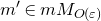 $m'\in mM_{O(\varepsilon )}$
. It follows that
$m'\in mM_{O(\varepsilon )}$
. It follows that $w\in {\mathbb{T}}_{T,b}$
and
$w\in {\mathbb{T}}_{T,b}$
and $m' \in \Theta$
, so
$m' \in \Theta$
, so $\gamma \in \Gamma \cap \mathcal{W}_{T,b}$ $(g_0,\varepsilon ,{\mathbb{T}},\Theta )$
.
$(g_0,\varepsilon ,{\mathbb{T}},\Theta )$
.
In the next Lemma5.10, we show that there are just as many primitive elements in $\Gamma \cap \mathcal{W}_{T,b}(g_0,\varepsilon ,\Theta )$
as nonprimitive elements. This is what allows us to consider only primitive elements in
$\Gamma \cap \mathcal{W}_{T,b}(g_0,\varepsilon ,\Theta )$
as nonprimitive elements. This is what allows us to consider only primitive elements in $\Gamma$
as in the joint equidistribution Theorem4.5. The proof uses Lemma5.9 and Proposition5.6 to get an estimate for
$\Gamma$
as in the joint equidistribution Theorem4.5. The proof uses Lemma5.9 and Proposition5.6 to get an estimate for $\#\Gamma _{\textrm{prim}} \cap \mathcal{W}_{T,b}(g_0,\varepsilon ,\Theta )$
.
$\#\Gamma _{\textrm{prim}} \cap \mathcal{W}_{T,b}(g_0,\varepsilon ,\Theta )$
.
Lemma 5.10.
Suppose $g_0 \in G$
with
$g_0 \in G$
with $\Gamma g_0M \in \operatorname {supp}\mathsf{m}_{\mathsf v}$
and
$\Gamma g_0M \in \operatorname {supp}\mathsf{m}_{\mathsf v}$
and $\operatorname {Vol}_M(\Theta ) \gt 0$
. Then for all sufficiently small
$\operatorname {Vol}_M(\Theta ) \gt 0$
. Then for all sufficiently small $\varepsilon \gt 0$
and sufficiently large
$\varepsilon \gt 0$
and sufficiently large $T$
, we have
$T$
, we have
 \begin{align*} \#\Gamma \cap (\mathcal{W}_{T,b}(g_0,\varepsilon ,\Theta )-\mathcal{W}_{2T/3,b}(g_0,\varepsilon ,\Theta ))\le \#\Gamma _{\textrm{prim}}\cap \mathcal{W}_{T,b}(g_0,\varepsilon ,\Theta ).\end{align*}
Proof. Let $\Gamma _{\textrm{prim}^k}=\{\sigma ^k:\sigma \in \Gamma _{\textrm{prim}}\}$
. We observe that
$\Gamma _{\textrm{prim}^k}=\{\sigma ^k:\sigma \in \Gamma _{\textrm{prim}}\}$
. We observe that
 \begin{align*} & \#\Gamma _{\textrm{prim}}\cap \mathcal{W}_{T,b}(g_0,\varepsilon ,{\mathbb{T}},\Theta )& \\ & =\#\Gamma \cap \mathcal{W}_{T,b}(g_0,\varepsilon ,{\mathbb{T}},\Theta )-\#\left (\bigcup _{k\ge 2}\Gamma _{\textrm{prim}^k}\cap \mathcal{W}_{T,b}(g_0,\varepsilon ,{\mathbb{T}},\Theta )\right ) \\ & \ge \#\Gamma \cap \mathcal{W}_{T,b}(g_0,\varepsilon ,{\mathbb{T}},\Theta )-\#\left (\bigcup _{k\ge 2}\Gamma \cap \mathcal{W}_{T/k,\hat {b}}(g_0,\varepsilon ,\hat {{\mathbb{T}}},\sqrt [k]{\Theta })\right ) \end{align*}
where $\sqrt [k]{\Theta }: = \{m \in M : m^k \in \Theta \}$
and
$\sqrt [k]{\Theta }: = \{m \in M : m^k \in \Theta \}$
and $\hat {{\mathbb{T}}}$
is the essential tube obtained from
$\hat {{\mathbb{T}}}$
is the essential tube obtained from $\mathbb{T}$
by replacing
$\mathbb{T}$
by replacing $\mathsf{K}$
with the convex hull of
$\mathsf{K}$
with the convex hull of $\mathsf{K}\cup \{0\}$
and
$\mathsf{K}\cup \{0\}$
and $\hat {b}$
is any continuous extension of
$\hat {b}$
is any continuous extension of $b$
to the convex hull of
$b$
to the convex hull of $\mathsf{K} \cup \{0\}$
. It suffices to show that for all sufficiently large
$\mathsf{K} \cup \{0\}$
. It suffices to show that for all sufficiently large $T$
, we have
$T$
, we have
 \begin{align} \#\left (\bigcup _{k\ge 2}\Gamma \cap \mathcal{W}_{T/k,\hat {b}}(g_0,\varepsilon ,\hat {{\mathbb{T}}},\sqrt [k]{\Theta })\right ) \le \#\Gamma \cap \mathcal{W}_{2T/3,b}(g_0,\varepsilon ,{\mathbb{T}},\Theta ). \end{align}
Since $\mathcal{W}_{T/k,\hat {b}}(g_0,\varepsilon ,\hat {{\mathbb{T}}},\sqrt [k]{\Theta }) \subset \mathcal{V}_{T/k,\hat {b}}(g_0,\varepsilon ,\hat {{\mathbb{T}}},\sqrt [k]{\Theta })$
and
$\mathcal{W}_{T/k,\hat {b}}(g_0,\varepsilon ,\hat {{\mathbb{T}}},\sqrt [k]{\Theta }) \subset \mathcal{V}_{T/k,\hat {b}}(g_0,\varepsilon ,\hat {{\mathbb{T}}},\sqrt [k]{\Theta })$
and $\Gamma \cap \mathcal{W}_{T/k,\hat {b}}(g_0,\varepsilon ,\hat {{\mathbb{T}}},\sqrt [k]{\Theta })$
is empty when
$\Gamma \cap \mathcal{W}_{T/k,\hat {b}}(g_0,\varepsilon ,\hat {{\mathbb{T}}},\sqrt [k]{\Theta })$
is empty when $T/k$
is sufficiently small, using Proposition5.6 we get
$T/k$
is sufficiently small, using Proposition5.6 we get
 \begin{align} \#\left (\bigcup _{k\ge 2}\Gamma \cap \mathcal{W}_{T/k,\hat {b}}(g_0,\varepsilon ,\hat {{\mathbb{T}}},\sqrt [k]{\Theta })\right )=O\left (T\frac {e^{ \delta _{\mathsf v} T/2}}{T^{({r}-1)/2}}\right)\!. \end{align}
Using Lemma5.9, Proposition5.6 and $\operatorname {Vol}_M(\Theta ) \gt 0$
, we have
$\operatorname {Vol}_M(\Theta ) \gt 0$
, we have
 \begin{align} \#\Gamma \cap \mathcal{W}_{2T/3,b}(g_0,\varepsilon ,{\mathbb{T}},\Theta ) \ge O\left (\frac {e^{2\delta _{\mathsf v} T/3}}{T^{({r}-1)/2}}\right)\!. \end{align}
Joint equidistribution
Our next goal is to prove Theorem4.4. For each $T\gt 0$
, we define a Radon measure
$T\gt 0$
, we define a Radon measure $\eta _T$
on
$\eta _T$
on $\Omega \times [M]$
by the following: for
$\Omega \times [M]$
by the following: for $f\in\textrm{C}_{\textrm{c}}(\Omega )$
and
$f\in\textrm{C}_{\textrm{c}}(\Omega )$
and $\varphi \in \textrm{Cl}(M)$
, let
$\varphi \in \textrm{Cl}(M)$
, let
 \begin{align*} \eta _{T}(f\otimes \varphi )=\sum _{ [\gamma ] \in [\Gamma _{\textrm{prim}}],\, \lambda (\gamma ) \in {\mathbb{T}}_{T,b}} \int _{C_\gamma } f \cdot \varphi (m(\gamma )). \end{align*}
We will prove Theorem4.4 by using the asymptotic in Proposition5.6. Let $g_0 \in G$
with
$g_0 \in G$
with $\Gamma g_0M \in \operatorname {supp}\mathsf{m}_{\mathsf v}$
,
$\Gamma g_0M \in \operatorname {supp}\mathsf{m}_{\mathsf v}$
, $\Theta \subset M_{\Gamma}$
be a conjugation-invariant Borel subset with
$\Theta \subset M_{\Gamma}$
be a conjugation-invariant Borel subset with $\operatorname {Vol}_M(\Theta ) \gt 0$
and
$\operatorname {Vol}_M(\Theta ) \gt 0$
and $\operatorname {Vol}_M(\partial \Theta ) = 0$
and let
$\operatorname {Vol}_M(\partial \Theta ) = 0$
and let $\varepsilon \gt 0$
be sufficiently small as in Proposition5.6.
$\varepsilon \gt 0$
be sufficiently small as in Proposition5.6.
Lemma 5.11 (Reference Chow and FrommCF23, Lemma 6.3). For all sufficiently large $T\gt 1$
, we have
$T\gt 1$
, we have
 \begin{align*} \eta _{T}(\tilde {\mathcal{B}}(g_0,\varepsilon )\otimes \Theta )=b_{{r}}(\varepsilon )\cdot \#(\Gamma _{\textrm{prim}}\cap \mathcal{W}_{T,b}(g_0,\varepsilon ,{\mathbb{T}},\Theta )).\end{align*}
In view of Lemma5.11, we can now use Lemmas5.9 and 5.10 to prove the following lemma comparing $\eta _T$
with
$\eta _T$
with $\mathcal{V}_{T,b}$
.
$\mathcal{V}_{T,b}$
.
Lemma 5.12 (Comparison Lemma). For all sufficiently large $T\gt 1$
, we have
$T\gt 1$
, we have
 \begin{align*} b_{{r}}(\varepsilon )\cdot \#\Gamma \cap (\mathcal{V}_{T,b_\varepsilon ^-}(g_0,\varepsilon -O(\varepsilon e^{-2CT/3})),{\mathbb{T}}^-_\varepsilon ,\Theta ^-_\varepsilon )-\mathcal{V}_{2T/3,b}(g_0,\varepsilon ,{\mathbb{T}},\Theta )) \\ \le \eta _{T}(\tilde {\mathcal{B}}(g_0,\varepsilon )\otimes \Theta )\le b_{{r}}(\varepsilon )\cdot \#\Gamma \cap \mathcal{V}_{T,b}(g_0,\varepsilon ,{\mathbb{T}},\Theta ) \end{align*}
where $C$
,
$C$
, $\Theta ^-_\varepsilon$
and
$\Theta ^-_\varepsilon$
and ${\mathbb{T}}^-_{T,\varepsilon }$
are as in Lemma
5.9
.
${\mathbb{T}}^-_{T,\varepsilon }$
are as in Lemma
5.9
.
Proof. The upper bound follows directly from Lemma5.11 and the inclusion $\Gamma \cap \mathcal{W}_T(g_0,\varepsilon ,{\mathbb{T}},\Theta ) \subset \Gamma \cap \mathcal{V}_T(g_0,\varepsilon ,{\mathbb{T}},\Theta )$
. The lower bound follows by using Lemmas5.11, 5.10, and 5.9:
$\Gamma \cap \mathcal{W}_T(g_0,\varepsilon ,{\mathbb{T}},\Theta ) \subset \Gamma \cap \mathcal{V}_T(g_0,\varepsilon ,{\mathbb{T}},\Theta )$
. The lower bound follows by using Lemmas5.11, 5.10, and 5.9:
 \begin{align*} & \eta _{T}(\tilde {\mathcal{B}}(g_0,\varepsilon )\otimes \Theta ) \\ & = b_{{r}}(\varepsilon )\#(\Gamma _{\textrm{prim}}\cap \mathcal{W}_{T,b}(g_0,\varepsilon ,{\mathbb{T}},\Theta )) \\ & \ge b_{{r}}(\varepsilon )\#\Gamma \cap (\mathcal{W}_{T,b}(g_0,\varepsilon ,{\mathbb{T}},\Theta )-\mathcal{W}_{2T/3,b}(g_0,\varepsilon ,{\mathbb{T}},\Theta )) \\ & \ge b_{{r}}(\varepsilon )\#\Gamma \cap (\mathcal{V}_{T,b_\varepsilon ^-}(g_0,\varepsilon -O(\varepsilon e^{-2CT/3})),{\mathbb{T}}^-_\varepsilon ,\Theta ^-_\varepsilon )-\mathcal{V}_{2T/3,b}(g_0,\varepsilon ,{\mathbb{T}},\Theta )).\\[-8pt]& \end{align*}
Combining Proposition5.6 and Lemma5.12, we obtain the following asymptotic for $\eta _{T}(\tilde {\mathcal{B}}(g_0,\varepsilon )\otimes \Theta )$
.
$\eta _{T}(\tilde {\mathcal{B}}(g_0,\varepsilon )\otimes \Theta )$
.
Proposition 5.13. We have
 \begin{align*} \eta _{T}(\tilde {\mathcal{B}}(g_0,\varepsilon )\otimes \Theta ) =c({\mathsf v}, b) (\mathsf{m}_{\mathsf v}(\tilde {\mathcal{B}}(g_0,\varepsilon ))\operatorname {Vol}_M(\Theta ) (1+O(\varepsilon )) +o_T(1))\frac {e^{\delta _{\mathsf v} T}}{T^{({r}-1)/2}} \end{align*}
where $c({\mathsf v},b)$
is as in (
4.2
).
$c({\mathsf v},b)$
is as in (
4.2
).
Proof. Using the asymptotics from Proposition5.6 in the inequality in Lemma5.12 gives
 \begin{align*} \eta _{T}(\tilde {\mathcal{B}}(g_0,\varepsilon )\otimes \Theta ) \le c({\mathsf v},b) (\mathsf{m}_{\mathsf v}(\tilde {\mathcal{B}}(g_0,\varepsilon ))\operatorname {Vol}_M(\Theta ) (1+O(\varepsilon )) +o_T(1))\frac {e^{\delta _{\mathsf v} T}}{ T^{({r}-1)/2}} \end{align*}
and
 \begin{align*} & \eta _{T}(\tilde {\mathcal{B}}(g_0,\varepsilon )\otimes \Theta ) \\ & \ge b_{{r}}(\varepsilon )\cdot \#\Gamma \cap \left (\mathcal{V}_{T,b_\varepsilon ^-}(g_0,\varepsilon -O(\varepsilon e^{-2CT/3})),{\mathbb{T}}^-_\varepsilon ,\Theta ^-_\varepsilon )-\mathcal{V}_{2T/3,b}(g_0,\varepsilon ,{\mathbb{T}},\Theta )\right ) \\ & = c({\mathsf v},b_\varepsilon ^-) \\ & \cdot \left (\frac {b_{{r}}(\varepsilon )\mathsf{m}_{\mathsf v}\Big(\tilde {\mathcal{B}}\Big(g_0,\varepsilon -O\Big(\varepsilon e^{-\tfrac {2CT}{3}}\Big)\Big)\Big)}{b_{{r}}\Big(\varepsilon -O\Big(\varepsilon e^{-\tfrac {2CT}{3}}\Big)\Big)}\operatorname {Vol}_M(\Theta ^-_\varepsilon )(1+O(\varepsilon ))+o_T(1) \right )\frac {e^{\delta _{\mathsf v} T}}{T^{({r}-1)/2}} \\ & \qquad \qquad - c({\mathsf v},b)(\mathsf{m}_{\mathsf v}(\tilde {\mathcal{B}}(g_0,\varepsilon ))\operatorname {Vol}_M(\Theta ) (1+O(\varepsilon ))+o_T(1))\frac {e^{2\delta _{\mathsf v} T/3}}{(2T/3)^{({r}-1)/2}} \\ & = c({\mathsf v},b)(\mathsf{m}_{\mathsf v}(\tilde {\mathcal{B}}(g_0,\varepsilon ))\operatorname {Vol}_M(\Theta ) (1+O(\varepsilon ))+o_T(1))\frac {e^{\delta _{\mathsf v} T}}{ T^{({r}-1)/2}}. \end{align*}
Proofs of Theorems4.4 and 4.5
The left-hand side of the asymptotic formula of Theorem4.4 is precisely $\eta _{T}(f\otimes \varphi )$
. Theorem4.4 now follows from Proposition5.13 and a standard partition of unity argument ([Reference Margulis, Mohammadi and OhMMO14, Theorem 5.17], [Reference Chow and FrommCF23, Theorem 6.12]).
$\eta _{T}(f\otimes \varphi )$
. Theorem4.4 now follows from Proposition5.13 and a standard partition of unity argument ([Reference Margulis, Mohammadi and OhMMO14, Theorem 5.17], [Reference Chow and FrommCF23, Theorem 6.12]).
We now deduce Theorem4.5 from Theorem4.4. Let $f \in \textrm{C}_{\textrm{c}}(\Omega )$
and
$f \in \textrm{C}_{\textrm{c}}(\Omega )$
and $\varphi \in \textrm{Cl}(M)$
. Since
$\varphi \in \textrm{Cl}(M)$
. Since $\psi _{\mathsf v}(w) \le T + \sup b$
for all
$\psi _{\mathsf v}(w) \le T + \sup b$
for all $w \in {\mathbb{T}}_{T,b}$
, we have
$w \in {\mathbb{T}}_{T,b}$
, we have
 \begin{align*} (T+\sup b)\sum _{ [\gamma ] \in [\Gamma _{\textrm{prim}}], \, \lambda (\gamma ) \in {\mathbb{T}}_{T,b}} \frac {\int _{C_\gamma } f}{\psi _{\mathsf v}(\lambda (\gamma ))}\varphi (m(\gamma )) \ge \eta _{T}(f\otimes \varphi ).\end{align*}
On the other hand, for any $\varepsilon \gt 0$
, we have
$\varepsilon \gt 0$
, we have
 \begin{align*} & \tfrac {1}{e^{\delta _{\mathsf v} T} T^{(1-{r})/2}}\sum _{ [\gamma ] \in [\Gamma _{\textrm{prim}}] ,\, \lambda (\gamma ) \in {\mathbb{T}}_{T,b}} \frac {\int _{C_\gamma } f}{\psi _{\mathsf v}(\lambda (\gamma ))}\varphi (m(\gamma )) \\[5pt] & =\tfrac {1}{e^{\delta _{\mathsf v} T} T^{(1-{r})/2}}\sum _{ [\gamma ] \in [\Gamma _{\textrm{prim}}] ,\, \lambda (\gamma ) \in {\mathbb{T}}_{(1-\varepsilon )T,b}} \frac {\int _{C_\gamma } f}{\psi _{\mathsf v}(\lambda (\gamma ))}\varphi (m(\gamma )) \\[5pt] & \qquad \qquad +\tfrac {1}{e^{\delta _{\mathsf v} T} T^{(1-{r})/2}}\sum _{ [\gamma ] \in [\Gamma _{\textrm{prim}}] ,\, \lambda (\gamma ) \in {\mathbb{T}}_{T,b}-{\mathbb{T}}_{(1-\varepsilon )T,b}} \frac {\int _{C_\gamma } f}{\psi _{\mathsf v}(\lambda (\gamma ))}\varphi (m(\gamma )) \\[5pt] & \le \tfrac {1}{e^{\delta _{\mathsf v} T} T^{(1-{r})/2}}O(\eta _{(1-\varepsilon )T}(f\otimes \varphi )) \\[5pt] & \qquad \qquad +\tfrac {1}{e^{\delta _{\mathsf v} T} T^{(1-{r})/2}}\cdot \tfrac {1}{(1-\varepsilon )T+\inf b}\left (\eta _{T}(f\otimes \varphi )-\eta _{(1-\varepsilon )T}(f\otimes \varphi )\right ) \\[5pt] & =O(Te^{-\varepsilon \delta _{\mathsf v} T}) + \tfrac {1}{1-\varepsilon +(\inf b)/T}\cdot \tfrac {1}{e^{\delta _{\mathsf v} T}T^{(1-{r})/2}}\eta _{T}(f\otimes \varphi ). \end{align*}
Using the asymptotic for $\eta _T(f\otimes \varphi )$
from Theorem4.4 in both inequalities, taking
$\eta _T(f\otimes \varphi )$
from Theorem4.4 in both inequalities, taking $T\to \infty$
and
$T\to \infty$
and $\varepsilon \to 0$
gives the desired asymptotic.
$\varepsilon \to 0$
gives the desired asymptotic.
6. Cartan projections in tubes
In this section, we prove an asymptotic for the number of Cartan projections of a Zariski dense Anosov subgroup in a given essential tube (Theorem6.1). Recall the Cartan projection $\mu :G\to {\mathfrak a}^+$
.
$\mu :G\to {\mathfrak a}^+$
.
Cartan projections in tubes
Let $\Gamma \lt G$
be a Zariski dense Anosov subgroup. Fix
$\Gamma \lt G$
be a Zariski dense Anosov subgroup. Fix

Recall that associated to $\mathsf v$
are the
$\mathsf v$
are the $\Gamma$
-conformal measures
$\Gamma$
-conformal measures $\nu =\nu _{{\mathsf v}}$
and
$\nu =\nu _{{\mathsf v}}$
and $\nu _{{\operatorname {i}}}=\nu _{\mathsf{i}({\mathsf v})}$
. Fix Borel subsets
$\nu _{{\operatorname {i}}}=\nu _{\mathsf{i}({\mathsf v})}$
. Fix Borel subsets $\Xi _1 ,\Xi _2\subset K$
such that
$\Xi _1 ,\Xi _2\subset K$
such that $\Xi _1 M=\Xi _1$
,
$\Xi _1 M=\Xi _1$
, $M \Xi _2 =\Xi _2$
, and
$M \Xi _2 =\Xi _2$
, and $\nu (\partial \Xi _1) = \nu _{\mathsf{i}}(\partial \Xi _2^{-1}) = 0$
. We will abuse notation and also view
$\nu (\partial \Xi _1) = \nu _{\mathsf{i}}(\partial \Xi _2^{-1}) = 0$
. We will abuse notation and also view $\Xi _1, \Xi _2^{-1}$
as subsets of
$\Xi _1, \Xi _2^{-1}$
as subsets of $\mathcal{F}\cong K/M$
.
$\mathcal{F}\cong K/M$
.
Recall the notation:
 \begin{align*} {\mathbb{T}}_{T,b}={\mathbb{T}}_T(\mathsf{v},\mathsf{K},b)=\{t\mathsf{v}+u \in \mathcal{L} : 0 \le t \le T+b(u), \, u \in \mathsf{K}\}.\end{align*}
Theorem 6.1 (Cartan projections in tubes). We have as $T \to \infty$
,
$T \to \infty$
,
 \begin{align*} \#\Gamma \cap \Xi _1\exp ({\mathbb{T}}_{T,b})\Xi _2 \sim c({\mathsf v}, b) \cdot \nu (\Xi _1) \cdot \nu _{\mathsf{i}}(\Xi _2^{-1})\frac {e^{\delta _{\mathsf v} T}}{ T^{({r}-1)/2}} \end{align*}
where $c({\mathsf v}, b)$
is as in (
4.2
).
$c({\mathsf v}, b)$
is as in (
4.2
).
An immediate corollary is as follows.
Corollary 6.2.
As $T \to \infty$
we have
$T \to \infty$
we have
 \begin{align*} \#\{\gamma \in \Gamma :\mu (\gamma ) \in {\mathbb{T}}_{T,b}\} \sim c({\mathsf v}, b) \, \cdot \frac {e^{\delta _{\mathsf v} T}}{ T^{({r}-1)/2}}.\end{align*}
Corollary6.2 together with Theorem4.2 now implies the following.
Corollary 6.3.
We have as $T \to \infty$
,
$T \to \infty$
,
 \begin{align*} \frac {\#\{\gamma \in \Gamma : \mu (\gamma ) \in {\mathbb{T}}_{T,b}\} }{\#\{[\gamma ] \in [\Gamma ]:\lambda (\gamma ) \in {\mathbb{T}}_{T,b}\} }\sim \frac {[M:M_{\Gamma} ]}{|m_{\mathcal{X}_{\mathsf v}}|} T.\end{align*}
Proof of Theorem6.1
In [Reference Edwards, Lee and OhELO23, Section 9], an asymptotic for the number of Cartan projections in cones was obtained for certain special kind of norms. In principle, it is not clear whether their result can be extended to deal with the Euclidean norm counting in cones. However, for counting in tubes, the fact that the tubes contain only one direction implies that all norms are essentially the same restricted to tubes. Together with integral computation in Lemma5.4, this enables us to use the approach of [Reference Edwards, Lee and OhELO23, Section 9] to prove Theorem6.1. To be precise, consider the following bounded subset for each $T$
: let
$T$
: let
 \begin{align*} R_{T,b} = R_T(\Xi _1,\Xi _2,{\mathbb{T}},b) = \Xi _1\exp ({\mathbb{T}}_{T,b})\Xi _2.\end{align*}
For a given bounded subset $B\subset G$
, define the counting function
$B\subset G$
, define the counting function $F_{B}: \Gamma \backslash G \to {\mathbb R}$
by
$F_{B}: \Gamma \backslash G \to {\mathbb R}$
by
 \begin{align*} F_B(\Gamma g) = \sum _{\gamma \in \Gamma }\unicode {x1D7D9}_B(\gamma g) = \# (\Gamma \cap Bg^{-1}).\end{align*}
We claim that for any $\Psi \in C_{\textrm{c}}(\Gamma \backslash G)$
, we have
$\Psi \in C_{\textrm{c}}(\Gamma \backslash G)$
, we have
 \begin{align*} \lim \limits _{T\to \infty }\frac {\langle F_{R_{T,b}}, \Psi \rangle }{e^{\delta _{\mathsf v} T} T^{(1-{r})/2}} = c({\mathsf v}, b) \cdot \nu (\Xi _1) \cdot \mathsf{m}^{\textrm{BR}}_{\mathsf v}(\Psi \ast \unicode {x1D7D9}_{\Xi _2})\end{align*}
where $\Psi \ast \unicode {x1D7D9}_{\Xi _2}(x) = \int _{\Xi _2}\Psi (xk)\,dk$
.
$\Psi \ast \unicode {x1D7D9}_{\Xi _2}(x) = \int _{\Xi _2}\Psi (xk)\,dk$
.
The Haar measure $dg$
on
$dg$
on $G$
can be written
$G$
can be written
 \begin{align*} dg = \zeta (w) \,dk_1d\,k_2\,dw\end{align*}
where $g=k_1\exp (w)k_2 \in K\exp (\mathfrak{a}^+)K$
,
$g=k_1\exp (w)k_2 \in K\exp (\mathfrak{a}^+)K$
, $\zeta (w) = \prod _{\alpha \in \Phi ^+}2\sinh (\alpha (w))$
; here
$\zeta (w) = \prod _{\alpha \in \Phi ^+}2\sinh (\alpha (w))$
; here $dk$
and
$dk$
and $dw$
denote the Haar measures on
$dw$
denote the Haar measures on $K$
and
$K$
and $\mathfrak{a}^+$
respectively ([Reference KnappKna86, Proposition 5.28], c.f. [Reference Oh and ShahOS13, Theorem 8.1] for the normalization).
$\mathfrak{a}^+$
respectively ([Reference KnappKna86, Proposition 5.28], c.f. [Reference Oh and ShahOS13, Theorem 8.1] for the normalization).
Using this formula as in the proof of [Reference Edwards, Lee and OhELO23, Proposition 9.10] and the decomposition of ${\mathbb{T}}_{T,b}$
as in Lemma5.4, we have
${\mathbb{T}}_{T,b}$
as in Lemma5.4, we have
 \begin{align*} \frac {\langle F_{R_{T,b}}, \Psi \rangle }{e^{\delta _{\mathsf v} T}T^{(1-{r})/2}} &= \frac {1}{e^{\delta _{\mathsf v} T}T^{(1-{r})/2}}\int _{\ker \psi _{\mathsf v}}\int _{R_T(u)}\bigg (e^{\delta _{\mathsf v} t}e^{-2\rho (t{\mathsf v}+\sqrt {t}u)}\zeta (t{\mathsf v}+\sqrt {t}u) \\ &\quad \cdot t^{({r}-1)/2}e^{2\rho (t{\mathsf v}+\sqrt {t}u)-\delta _{\mathsf v} t}\int _{k \in \Xi _1}\Psi \ast \unicode {x1D7D9}_{\Xi _2}(\Gamma ka_{t{\mathsf v}+\sqrt {t}u})\,d(\Gamma k)\bigg )\,dt\,du. \end{align*}
Note that
 \begin{align*} \lim _{t\to \infty }e^{-2\rho (t{\mathsf v}+\sqrt {t}u)}\zeta (t{\mathsf v}+\sqrt {t}u)=1 .\end{align*}
By [Reference Edwards, Lee and OhELO23, Proposition 8.11], we have
 \begin{align} \lim _{t\to \infty }t^{({r}-1)/2}e^{2\rho (t{\mathsf v}+\sqrt {t}u)-\delta _{\mathsf v} t}\int _{ k \in \Xi _1}\Psi \ast \unicode {x1D7D9}_{\Xi _2}(\Gamma ka_{t{\mathsf v}+\sqrt {t}u})\,d(\Gamma k) \\ = \frac {\kappa _{\mathsf v}}{|m_{\mathcal{X}_{\mathsf v}}|} e^{-I(u)}\nu ^K(\Xi _1)\mathsf{m}^{\textrm{BR}}_{\mathsf v}(\Psi \ast \unicode {x1D7D9}_{\Xi _2}).\nonumber \end{align}
Then we can apply the Lebesgue dominated convergence theorem, (6.1) and Lemma5.4 to conclude that
 \begin{align*} \begin{aligned}[b] & \lim \limits _{T\to \infty }\frac {\langle F_{R_{T,b}}, \Psi \rangle }{e^{\delta _{\mathsf v} T}T^{(1-{r})/2}} \\ & = \lim \limits _{T\to \infty }\frac {1}{e^{\delta _{\mathsf v} T}T^{(1-{r})/2}}\int _{\ker \psi _{\mathsf v}}\int _{R_T(u)}e^{\delta _{\mathsf v} t}\frac {\kappa _{\mathsf v}}{|m_{\mathcal{X}_{\mathsf v}}|} e^{-I(u)}\nu (\Xi _1)\mathsf{m}^{\textrm{BR}}_{\mathsf v}(\Psi \ast \unicode {x1D7D9}_{\Xi _2})\,dt\,du \\ & = \frac {\kappa _{\mathsf v}}{\delta _{\mathsf v}|m_{\mathcal{X}_{\mathsf v}}|}\int _{\mathsf{K}} e^{\delta _{\mathsf v} b(u)}\,du\cdot \nu (\Xi _1)\mathsf{m}^{\textrm{BR}}_{\mathsf v}(\Psi \ast \unicode {x1D7D9}_{\Xi _2}). \end{aligned} \end{align*}
This proves the claim. Theorem6.1 is then proved in the same way as [Reference Edwards, Lee and OhELO23, Corollary 9.21].
7. Applications to correlations of spectra and the growth indicator
In this section, we prove Theorem1.1 as an application of Theorem4.2 and Corollary6.2. For this section, let $G_1, \ldots , G_d$
be connected simple real algebraic groups of rank one. For each
$G_1, \ldots , G_d$
be connected simple real algebraic groups of rank one. For each $i$
, we use the same notations for Lie subgroups of
$i$
, we use the same notations for Lie subgroups of $G_i$
as introduced in Section 2 but with
$G_i$
as introduced in Section 2 but with $i$
as subscript. For each
$i$
as subscript. For each $i$
, let
$i$
, let $(X_i=G_i/K_i, \mathsf d_i)$
denote the associated Riemannian symmetric space. Let
$(X_i=G_i/K_i, \mathsf d_i)$
denote the associated Riemannian symmetric space. Let $q_i \in X_i$
be the point stabilized by a
$q_i \in X_i$
be the point stabilized by a $K_i$
. We identify each
$K_i$
. We identify each $\mathfrak{a}_i^+$
with
$\mathfrak{a}_i^+$
with $[0,\infty )$
using the induced norm on
$[0,\infty )$
using the induced norm on $\mathfrak{a}_i$
.
$\mathfrak{a}_i$
.
Correlations of length spectra and correlations of displacement spectra for convex-cocompact manifolds
We give an application of Theorem4.2 to the correlations of length spectra. We also give an application of Theorem6.1 to the correlations of displacement spectra in the same setting.
Let $\rho =(\rho _1,\ldots ,\rho _d):\Gamma \to G_1 \times \ldots \times G_d$
be a
$\rho =(\rho _1,\ldots ,\rho _d):\Gamma \to G_1 \times \ldots \times G_d$
be a $d$
-tuple of faithful representations of a finitely generated group
$d$
-tuple of faithful representations of a finitely generated group $\Gamma$
whose images are Zariski-dense convex-cocompact subgroups. For each
$\Gamma$
whose images are Zariski-dense convex-cocompact subgroups. For each $i=1.\ldots ,d$
, each conjugacy class
$i=1.\ldots ,d$
, each conjugacy class $[\rho _i(\gamma )] \in [\rho _i(\Gamma )]$
corresponds to a unique closed geodesic in the convex-cocompact manifold
$[\rho _i(\gamma )] \in [\rho _i(\Gamma )]$
corresponds to a unique closed geodesic in the convex-cocompact manifold $\rho _i(\Gamma ){\backslash } X_i$
whose length
$\rho _i(\Gamma ){\backslash } X_i$
whose length $\ell _{\rho _i(\gamma )}$
is equal to the Jordan projection of
$\ell _{\rho _i(\gamma )}$
is equal to the Jordan projection of $\rho _i(\gamma )$
. We denote by
$\rho _i(\gamma )$
. We denote by $[m_{\rho _i(\gamma )}] \in [M_i]$
the holonomy class associated to
$[m_{\rho _i(\gamma )}] \in [M_i]$
the holonomy class associated to $\rho _i(\gamma )$
. Define the spectrum cone
$\rho _i(\gamma )$
. Define the spectrum cone $\mathcal{L}_\rho$
of
$\mathcal{L}_\rho$
of $\rho$
as the smallest closed cone in
$\rho$
as the smallest closed cone in ${\mathbb R}^d$
containing the set
${\mathbb R}^d$
containing the set
 \begin{align*} \{(\ell _{\rho _1(\gamma )},\ldots ,\ell _{\rho _d(\gamma )}): \gamma \in \Gamma \}.\end{align*}
Theorem 7.1 (Correlations of length spectra and holonomies). For any ${\mathsf v} = (v_1,\ldots ,v_d) \in \textrm {int}\mathcal{L}_\rho$
, there exists
${\mathsf v} = (v_1,\ldots ,v_d) \in \textrm {int}\mathcal{L}_\rho$
, there exists $\delta _\rho ({\mathsf v})\gt 0$
such that for any
$\delta _\rho ({\mathsf v})\gt 0$
such that for any ${\varepsilon }_1,\ldots ,{\varepsilon }_d\gt 0$
and for any conjugation-invariant Borel sets
${\varepsilon }_1,\ldots ,{\varepsilon }_d\gt 0$
and for any conjugation-invariant Borel sets $\Theta _i \subset M_i$
with null boundaries, we have as
$\Theta _i \subset M_i$
with null boundaries, we have as $T\to \infty$
,
$T\to \infty$
,
 \begin{align} \#\{[\gamma ]\in [\Gamma ]: v_iT \le \ell _{\rho _i(\gamma )} \le v_iT+{\varepsilon }_i,\, m_{\rho _i(\gamma )}\in \Theta _i, \; 1\le i\le d\} \\ \sim c \frac {e^{\delta _\rho ({\mathsf v})T}}{ T^{(d+1)/{2}}} \prod _{i=1}^d\operatorname {Vol}_{M_i}(\Theta _i) \nonumber \end{align}
for some constant $c=c({\mathsf v},\varepsilon _1,\ldots ,{\varepsilon }_d)\gt 0$
. Moreover, we have
$c=c({\mathsf v},\varepsilon _1,\ldots ,{\varepsilon }_d)\gt 0$
. Moreover, we have
 \begin{align} \delta _\rho ({\mathsf v}) \le \min _i \delta _{\rho _i(\Gamma )}v_i. \end{align}
If $d\ge 2$
, we also have
$d\ge 2$
, we also have
 \begin{align} \delta _\rho ({\mathsf v}) \lt \frac {1}{d}\sum _{i=1}^d\delta _{\rho _i(\Gamma )}v_i. \end{align}
Theorem 7.2 (Correlations of displacements). For any ${\mathsf v} = (v_1,\ldots ,v_d) \in \textrm {int}\mathcal{L}_\rho$
and for any
${\mathsf v} = (v_1,\ldots ,v_d) \in \textrm {int}\mathcal{L}_\rho$
and for any ${\varepsilon }_1,\ldots ,{\varepsilon }_d\gt 0$
, as
${\varepsilon }_1,\ldots ,{\varepsilon }_d\gt 0$
, as $T\to \infty$
,
$T\to \infty$
,
 \begin{align*} \#\{\gamma \in \Gamma : v_iT\le \mathsf{d}_i(\rho _i(\gamma ) q_i,q_i) \le v_iT+{\varepsilon }_i, \; 1 \le i \le d\} \sim c' c \frac {e^{\delta _\rho ({\mathsf v})T}}{ T^{{(d-1)}/{2}}} \end{align*}
where $c=c({\mathsf v},\varepsilon _1,\ldots ,{\varepsilon }_d)$
is as in Theorem
7.1
and
$c=c({\mathsf v},\varepsilon _1,\ldots ,{\varepsilon }_d)$
is as in Theorem
7.1
and $c' = c'({\mathsf v},\rho ) \gt 0$
.
$c' = c'({\mathsf v},\rho ) \gt 0$
.
Remark 7.3. We say that $\rho _1,\ldots ,\rho _d$
are
$\rho _1,\ldots ,\rho _d$
are $ $
independent from each other if
$ $
independent from each other if $\rho _j\circ \rho _i^{-1}:\rho _i(\Gamma )\to \rho _j(\Gamma )$
does not extend to a Lie group isomorphism
$\rho _j\circ \rho _i^{-1}:\rho _i(\Gamma )\to \rho _j(\Gamma )$
does not extend to a Lie group isomorphism $G_i\to G_j$
for all
$G_i\to G_j$
for all $i\ne j$
. In the case that
$i\ne j$
. In the case that $\rho _1,\ldots ,\rho _d$
are not independent from each other, we observe in the proof of Theorem 7.1 that
$\rho _1,\ldots ,\rho _d$
are not independent from each other, we observe in the proof of Theorem 7.1 that $\mathcal{L}_\rho$
has empty interior and hence the above theorems are vacuous in that case.
$\mathcal{L}_\rho$
has empty interior and hence the above theorems are vacuous in that case.
Proofs of Theorems7.1 and 7.2
The self-joining of $\Gamma$
via
$\Gamma$
via $\rho =(\rho _1,\ldots ,\rho _d)$
is the discrete subgroup
$\rho =(\rho _1,\ldots ,\rho _d)$
is the discrete subgroup
 \begin{align} \Gamma _\rho =\{ \rho (\gamma )=(\rho _1(\gamma ), \ldots , \rho _d(\gamma )):\gamma \in \Gamma \} \lt \prod _{i=1}^dG_i. \end{align}
By Remark7.3, it suffices to consider the case where $\rho _1,\ldots ,\rho _d$
are independent from each other. Since
$\rho _1,\ldots ,\rho _d$
are independent from each other. Since $\rho _i(\Gamma )$
is a Zariski-dense subgroup of
$\rho _i(\Gamma )$
is a Zariski-dense subgroup of $G_i$
for each
$G_i$
for each $1\le i\le d$
, it follows that
$1\le i\le d$
, it follows that $\Gamma _\rho$
is Zariski-dense in
$\Gamma _\rho$
is Zariski-dense in $\prod _{i=1}^d G_i$
(cf. [Reference Kim and OhKO23, Lemma 4.1]). Since
$\prod _{i=1}^d G_i$
(cf. [Reference Kim and OhKO23, Lemma 4.1]). Since $\rho _i(\Gamma )$
is convex-cocompact for each
$\rho _i(\Gamma )$
is convex-cocompact for each $i=1,\ldots ,d$
,
$i=1,\ldots ,d$
, $\Gamma _\rho$
is an Anosov subgroup [Reference Guichard and WienhardGW12, Theorem 4.11]. Identifying
$\Gamma _\rho$
is an Anosov subgroup [Reference Guichard and WienhardGW12, Theorem 4.11]. Identifying $\mathfrak a$
with
$\mathfrak a$
with $\mathbb R^d$
, the Jordan projection of
$\mathbb R^d$
, the Jordan projection of $\rho (\gamma )\in \Gamma _\rho$
is
$\rho (\gamma )\in \Gamma _\rho$
is
 \begin{align*} \lambda (\rho (\gamma )) = (\ell _{\rho _1(\gamma )},\ldots ,\ell _{\rho _d(\gamma )}).\end{align*}
Hence $\mathcal{L}_{\rho } = \mathcal{L}_{\Gamma _\rho }$
and in particular
$\mathcal{L}_{\rho } = \mathcal{L}_{\Gamma _\rho }$
and in particular $\mathcal{L}_\rho$
has non-empty interior. We prove Theorem7.1 first using the above setup. For
$\mathcal{L}_\rho$
has non-empty interior. We prove Theorem7.1 first using the above setup. For $\gamma \in \Gamma$
, let
$\gamma \in \Gamma$
, let
 \begin{align*} m(\rho (\gamma )) = (m_{\rho _1(\gamma )},\ldots ,m_{\rho _d(\gamma )} ).\end{align*}
Truncated tubes.

We are interested in the asymptotic of
 \begin{align*} \#\bigg\{[\rho (\gamma )]\in [\Gamma _\rho ]: \lambda (\rho (\gamma )) \in \prod _{i=1}^d[v_iT, v_iT+{\varepsilon }_i], \; m(\rho (\gamma )) \in \prod _{i=1}^d\Theta _i\bigg\}.\end{align*}
Up to re-scaling, we may assume that ${\mathsf v}=(v_1, \ldots , v_d)$
is a unit vector in
${\mathsf v}=(v_1, \ldots , v_d)$
is a unit vector in $\textrm {int}\mathcal{L}_\rho$
. We claim that we can choose a compact subset
$\textrm {int}\mathcal{L}_\rho$
. We claim that we can choose a compact subset $\mathsf{K} \subset \ker \psi _{\mathsf v}$
and
$\mathsf{K} \subset \ker \psi _{\mathsf v}$
and $b_1,b_2\in C(\mathsf{K})$
such that the truncated tubes
$b_1,b_2\in C(\mathsf{K})$
such that the truncated tubes ${\mathbb{T}}_T({\mathsf v},\mathsf{K},b_1)$
and
${\mathbb{T}}_T({\mathsf v},\mathsf{K},b_1)$
and ${\mathbb{T}}_T({\mathsf v},\mathsf{K},b_2)$
satisfy
${\mathbb{T}}_T({\mathsf v},\mathsf{K},b_2)$
satisfy
 \begin{align*} {\mathbb{T}}_T({\mathsf v},\mathsf{K},b_1)- {\mathbb{T}}_T({\mathsf v},\mathsf{K},b_2) = \prod _{i=1}^d[v_iT,v_iT+{\varepsilon }_i]\end{align*}
for all sufficiently large $T$
. Consider the box
$T$
. Consider the box $\prod _{i=1}^d[0,{\varepsilon }_i]$
. Let
$\prod _{i=1}^d[0,{\varepsilon }_i]$
. Let $F_1 \subset {\mathbb R}^d$
(respectively
$F_1 \subset {\mathbb R}^d$
(respectively $F_2\subset {\mathbb R}^d$
) denote the union of the faces of the box not containing (respectively containing) the origin in
$F_2\subset {\mathbb R}^d$
) denote the union of the faces of the box not containing (respectively containing) the origin in ${\mathbb R}^d$
. Then it suffices to choose the truncated tubes so that (see Figure 4 for an illustration of the
${\mathbb R}^d$
. Then it suffices to choose the truncated tubes so that (see Figure 4 for an illustration of the $d=2$
case)
$d=2$
case)
 \begin{align*} & {\mathbb{T}}_T({\mathsf v},\mathsf{K},b_1) = [0,T]{\mathsf v} + F_1; & {\mathbb{T}}_T({\mathsf v},\mathsf{K},b_2) = [0,T]{\mathsf v} + F_2. \end{align*}
Equivalently, we need to choose $\mathsf{K}$
,
$\mathsf{K}$
, $b_1$
and
$b_1$
and $b_2$
so that
$b_2$
so that
 \begin{align*} & \{b_1(u){\mathsf v}+u:u \in \mathsf{K}\} = F_1; & \{b_2(u){\mathsf v}+u:u \in \mathsf{K}\} = F_2. \end{align*}
Noting that ${\mathbb R}^d = {\mathbb R}{\mathsf v}\oplus \ker \psi _{\mathsf v}$
, it suffices to check that for each
${\mathbb R}^d = {\mathbb R}{\mathsf v}\oplus \ker \psi _{\mathsf v}$
, it suffices to check that for each $i=1,2$
, the following holds:
$i=1,2$
, the following holds:
-
1. if
$w, w' \in F_i$
and
$w\ne w'$
, then
$w - w' \notin {\mathbb R}{\mathsf v}$
; -
2.
$F_1$
and
$F_2$
have the same image under the projection
${\mathbb R}{\mathsf v}\oplus \ker \psi _{\mathsf v} \to \ker \psi _{\mathsf v}$
.



For (1), suppose that $w=(w_1,\ldots ,w_d),w'=(w_1',\ldots ,w_d') \in F_i$
with
$w=(w_1,\ldots ,w_d),w'=(w_1',\ldots ,w_d') \in F_i$
with $w\ne w'$
. If
$w\ne w'$
. If $w$
and
$w$
and $w'$
are in the same face of the box, then there exists
$w'$
are in the same face of the box, then there exists $1 \le j \le d$
such that
$1 \le j \le d$
such that $w_j=w_j'$
. Then
$w_j=w_j'$
. Then $w_j-w_j'=0$
and hence
$w_j-w_j'=0$
and hence $w-w'$
cannot be parallel to
$w-w'$
cannot be parallel to ${\mathsf v} \in (0,\infty )^d$
. Suppose
${\mathsf v} \in (0,\infty )^d$
. Suppose $w$
and
$w$
and $w'$
are in different faces. If
$w'$
are in different faces. If $w,w' \in F_1$
, then there exist
$w,w' \in F_1$
, then there exist $1\le j,k\le d$
with
$1\le j,k\le d$
with $j\ne k$
such that
$j\ne k$
such that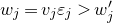 $w_j=v_j\varepsilon _j \gt w_j'$
and
$w_j=v_j\varepsilon _j \gt w_j'$
and $w_k' = v_k\varepsilon _k \gt w_k$
. Then
$w_k' = v_k\varepsilon _k \gt w_k$
. Then $w_j-w_j' \gt 0 \gt w_k-w_k'$
so
$w_j-w_j' \gt 0 \gt w_k-w_k'$
so $w-w'$
cannot be parallel to
$w-w'$
cannot be parallel to $\mathsf v$
. If
$\mathsf v$
. If $w,w' \in F_2$
, then there exist
$w,w' \in F_2$
, then there exist $1\le j,k\le d$
with
$1\le j,k\le d$
with $j\ne k$
such that
$j\ne k$
such that $w_j=0 \lt w_j'$
and
$w_j=0 \lt w_j'$
and $w_k' = 0 \lt w_k$
. Then
$w_k' = 0 \lt w_k$
. Then $w_j-w_j' \lt 0 \lt w_k-w_k'$
so
$w_j-w_j' \lt 0 \lt w_k-w_k'$
so $w-w'$
cannot be parallel to
$w-w'$
cannot be parallel to $\mathsf v$
. This establishes (1). For (2), note that since
$\mathsf v$
. This establishes (1). For (2), note that since $\mathsf v$
is not parallel to the faces of the box, any affine line parallel to
$\mathsf v$
is not parallel to the faces of the box, any affine line parallel to $\mathsf v$
that intersects
$\mathsf v$
that intersects $F_1 \cup F_2 - F_1 \cap F_2$
, must do so at exactly two points which cannot lie in the same
$F_1 \cup F_2 - F_1 \cap F_2$
, must do so at exactly two points which cannot lie in the same $F_i$
by (1). This establishes (2).
$F_i$
by (1). This establishes (2).
Let $\delta _\rho =\psi _{\Gamma _\rho }$
. Recall from Section 2 that
$\delta _\rho =\psi _{\Gamma _\rho }$
. Recall from Section 2 that $M_{\rho _i(\Gamma )}=M_i$
since
$M_{\rho _i(\Gamma )}=M_i$
since $G_i$
is rank one for each
$G_i$
is rank one for each $i=1,\ldots ,d$
. Applying Theorem4.2 to each tube
$i=1,\ldots ,d$
. Applying Theorem4.2 to each tube ${\mathbb{T}}_T({\mathsf v},\mathsf{K},b_i)$
, we have as
${\mathbb{T}}_T({\mathsf v},\mathsf{K},b_i)$
, we have as $T\to \infty$
 \begin{align*} \#\bigg\{[\gamma ] \in [\Gamma ]: \lambda (\rho (\gamma )) \in {\mathbb{T}}_T({\mathsf v},\mathsf{K},b_i), \; m(\rho (\gamma )) \in \prod _{i=1}^d\Theta _i\bigg\} \\ \sim C_i\frac {e^{\delta _{\rho }({\mathsf v})T}}{ T^{{(d-1)}/{2}}}\prod _{i=1}^d\operatorname {Vol}_{M_i}(\Theta _i) \end{align*}
where $\delta _\rho ({\mathsf v})=\psi _{\Gamma _\rho }({\mathsf v})$
and
$\delta _\rho ({\mathsf v})=\psi _{\Gamma _\rho }({\mathsf v})$
and $ C_i=\tfrac {\kappa _{\mathsf{v}}}{\psi _{\Gamma _\rho }({\mathsf v}) [M:M_{\Gamma} ]}\int _{\mathsf{K}} e^{\delta _{\rho }({\mathsf v}) b_i(u)} \, du$
for
$ C_i=\tfrac {\kappa _{\mathsf{v}}}{\psi _{\Gamma _\rho }({\mathsf v}) [M:M_{\Gamma} ]}\int _{\mathsf{K}} e^{\delta _{\rho }({\mathsf v}) b_i(u)} \, du$
for $i=1,2$
. Note that by construction,
$i=1,2$
. Note that by construction, $b_1 \gt b_2$
and hence
$b_1 \gt b_2$
and hence $C_1 \gt C_2$
. Then taking the difference gives
$C_1 \gt C_2$
. Then taking the difference gives
 \begin{align*} \#\bigg\{\rho (\gamma )\in [\Gamma _\rho ]: \lambda (\rho (\gamma )) \in \prod _{i=1}^d[v_iT, v_iT+{\varepsilon }_i], \; m(\rho (\gamma )) \in \prod _{i=1}^d\Theta _i\bigg\} \\ \sim (C_1-C_2) \frac {e^{\delta _\rho ({\mathsf v})T}}{ T^{{(d-1)}/{2}}}\prod _{i=1}^d\operatorname {Vol}_{M_i}(\Theta _i). \end{align*}
The upper bounds (7.2) and (7.3) are direct consequences of [Reference Kim, Minsky and OhKMO24, Theorem 1.4 and Corollary 1.6] since $\delta _\rho =\psi _{\Gamma _\rho }$
. This completes the proof of Theorem7.1 with
$\delta _\rho =\psi _{\Gamma _\rho }$
. This completes the proof of Theorem7.1 with $c = C_1-C_2$
.
$c = C_1-C_2$
.
Now we prove Theorem7.2. For each $i=1,\ldots ,d$
, we have
$i=1,\ldots ,d$
, we have $\mathsf{d}_i(\rho _i(\gamma ) q_i,q_i)=\|\mu (\rho _i(\gamma ))\|$
. Let
$\mathsf{d}_i(\rho _i(\gamma ) q_i,q_i)=\|\mu (\rho _i(\gamma ))\|$
. Let
 \begin{align*} \mu (\rho (\gamma ))=(\mathsf{d}_1(\rho _1(\gamma ) q_1,q_1),\ldots ,\mathsf{d}_d(\rho _i(\gamma ) q_d,q_d)).\end{align*}
We are now interested in the asymptotic of
 \begin{align*} \#\bigg\{\rho (\gamma )\in \Gamma _\rho : \mu (\rho (\gamma )) \in \prod _{i=1}^d[v_iT, v_iT+{\varepsilon }_i]\bigg\}.\end{align*}
Applying Corollary6.2 to the truncated tubes ${\mathbb{T}}_T({\mathsf v},\mathsf{K},b_1)$
and
${\mathbb{T}}_T({\mathsf v},\mathsf{K},b_1)$
and ${\mathbb{T}}_T({\mathsf v},\mathsf{K},b_2)$
as above, we obtain
${\mathbb{T}}_T({\mathsf v},\mathsf{K},b_2)$
as above, we obtain
 \begin{align*} \#\bigg\{\rho (\gamma )\in \Gamma _\rho : \mu (\rho (\gamma )) \in \prod _{i=1}^d[v_iT, v_iT+{\varepsilon }_i]\bigg\} \sim \tfrac {c}{|m_{\mathcal{X}_{\mathsf v}}|} \tfrac {e^{\delta _\rho ({\mathsf v})T}}{ T^{{(d-1)}/{2}}}\prod _{i=1}^d\operatorname {Vol}_{M_i}(\Theta _i). \end{align*}
This finishes the proof of Theorem7.2 with $c'= \tfrac {1}{|m_{\mathcal{X}_{\mathsf v}}|}$
.
$c'= \tfrac {1}{|m_{\mathcal{X}_{\mathsf v}}|}$
.
Correlation entropy rigidity
In view of Theorem7.1 on the correlations of length spectra, we define a correlation entropy function for a general $d$
-tuple of faithful representations
$d$
-tuple of faithful representations $\rho =(\rho _1,\ldots ,\rho _d):\Gamma \to G_1 \times \ldots \times G_d$
of a group
$\rho =(\rho _1,\ldots ,\rho _d):\Gamma \to G_1 \times \ldots \times G_d$
of a group $\Gamma$
.
$\Gamma$
.
Definition 7.4 (Correlation entropy function). For any $d$
-tuple of discrete faithful representations
$d$
-tuple of discrete faithful representations $\rho =(\rho _1,\ldots ,\rho _d):\Gamma \to G_1 \times \ldots \times G_d$
of a group
$\rho =(\rho _1,\ldots ,\rho _d):\Gamma \to G_1 \times \ldots \times G_d$
of a group $\Gamma$
, define the correlation entropy function
$\Gamma$
, define the correlation entropy function $\delta _\rho :{\mathbb R}^d \to [-\infty , \infty ]$
as follows. Given
$\delta _\rho :{\mathbb R}^d \to [-\infty , \infty ]$
as follows. Given ${\mathsf v} = (v_1,\ldots ,v_d) \in {\mathbb R}^d$
, define
${\mathsf v} = (v_1,\ldots ,v_d) \in {\mathbb R}^d$
, define
 \begin{align*} \delta _{\rho }({\mathsf v})=\liminf _{\max _i\varepsilon _i\to 0^+}\delta _{\rho }({\mathsf v},{\varepsilon }_1,\ldots ,{\varepsilon }_d) \end{align*}
where $\delta _{\rho }({\mathsf v},{\varepsilon }_1,\ldots ,{\varepsilon }_d)$
is given by
$\delta _{\rho }({\mathsf v},{\varepsilon }_1,\ldots ,{\varepsilon }_d)$
is given by

In the previous section, we have seen that for a $d$
-tuple
$d$
-tuple $\rho =(\rho _1,\ldots ,\rho _d):\Gamma \to G_1 \times \ldots \times G_d$
of faithful representations of a finitely generated group
$\rho =(\rho _1,\ldots ,\rho _d):\Gamma \to G_1 \times \ldots \times G_d$
of faithful representations of a finitely generated group $\Gamma$
whose images are Zariski-dense convex-cocompact subgroups, the correlation entropy
$\Gamma$
whose images are Zariski-dense convex-cocompact subgroups, the correlation entropy $\delta _\rho ({\mathsf v})$
is positive on
$\delta _\rho ({\mathsf v})$
is positive on $\textrm {int}\mathcal{L}_\rho$
when
$\textrm {int}\mathcal{L}_\rho$
when $\rho _1,\ldots ,\rho _d$
are independent from each other Theorem7.1. When
$\rho _1,\ldots ,\rho _d$
are independent from each other Theorem7.1. When $\rho _1,\ldots ,\rho _d$
are not independent from each other, we observed that
$\rho _1,\ldots ,\rho _d$
are not independent from each other, we observed that $\mathcal{L}_\rho$
has empty interior and, moreover,
$\mathcal{L}_\rho$
has empty interior and, moreover, $\delta _\rho = -\infty$
on
$\delta _\rho = -\infty$
on ${\mathbb R}^d-\mathcal{L}_\rho$
, so the set
${\mathbb R}^d-\mathcal{L}_\rho$
, so the set $\{{\mathsf v} \in {\mathbb R}^d: \delta _\rho ({\mathsf v}) \gt 0\}$
has empty interior.
$\{{\mathsf v} \in {\mathbb R}^d: \delta _\rho ({\mathsf v}) \gt 0\}$
has empty interior.
This phenomenon in fact holds without the convex-cocompact assumption.
Corollary 7.5 (Correlation entropy rigidity). Suppose $\rho = (\rho _1,\ldots ,\rho _d):\Gamma \to G_1\times \cdots \times G_d$
is a
$\rho = (\rho _1,\ldots ,\rho _d):\Gamma \to G_1\times \cdots \times G_d$
is a $d$
-tuple of discrete faithful representations of a countable group
$d$
-tuple of discrete faithful representations of a countable group $\Gamma$
with a Zariski-dense image. If
$\Gamma$
with a Zariski-dense image. If $\rho _1,\ldots ,\rho _d$
are independent from each other, then the interior of the set
$\rho _1,\ldots ,\rho _d$
are independent from each other, then the interior of the set $\{{\mathsf v} \in \mathbb R^d: \delta _\rho ({\mathsf v})\gt 0\}$
is a non-empty convex cone. Otherwise, the set
$\{{\mathsf v} \in \mathbb R^d: \delta _\rho ({\mathsf v})\gt 0\}$
is a non-empty convex cone. Otherwise, the set $\{{\mathsf v} \in \mathbb R^d: \delta _\rho ({\mathsf v})\gt 0\}$
has empty interior.
$\{{\mathsf v} \in \mathbb R^d: \delta _\rho ({\mathsf v})\gt 0\}$
has empty interior.
Proof. Corollary7.5 can be deduced from Theorem7.1 as follows. Using the same notation as in the previous subsection but without the convex-cocompact assumption on the representations $\rho _1,\ldots ,\rho _d$
, we can still consider the self-joining
$\rho _1,\ldots ,\rho _d$
, we can still consider the self-joining $\Gamma _\rho$
. Note that if
$\Gamma _\rho$
. Note that if ${\mathsf v} \in {\mathbb R}^d - \mathcal{L}_{\Gamma _\rho }$
, then clearly,
${\mathsf v} \in {\mathbb R}^d - \mathcal{L}_{\Gamma _\rho }$
, then clearly, $\delta _\rho ({\mathsf v},\varepsilon _1,\ldots ,\varepsilon _d) = - \infty$
for all
$\delta _\rho ({\mathsf v},\varepsilon _1,\ldots ,\varepsilon _d) = - \infty$
for all $\varepsilon _1,\ldots ,\varepsilon _d\gt 0$
.
$\varepsilon _1,\ldots ,\varepsilon _d\gt 0$
.
Suppose $\rho _1,\ldots ,\rho _d$
are independent from each other. Then
$\rho _1,\ldots ,\rho _d$
are independent from each other. Then $\Gamma _\rho$
is Zariski-dense and the limit cone
$\Gamma _\rho$
is Zariski-dense and the limit cone $\mathcal{L}_{\Gamma _\rho }$
has non-empty interior. Let
$\mathcal{L}_{\Gamma _\rho }$
has non-empty interior. Let ${\mathsf v}=(v_1,\ldots ,v_d) \in \textrm {int}\;\mathcal{L}_{\Gamma _\rho }$
. By [Reference BenoistBen97, Proposition 4.3], there exists a Zariski-dense Schottky subgroup
${\mathsf v}=(v_1,\ldots ,v_d) \in \textrm {int}\;\mathcal{L}_{\Gamma _\rho }$
. By [Reference BenoistBen97, Proposition 4.3], there exists a Zariski-dense Schottky subgroup $\Gamma ' \lt \Gamma _\rho$
such that
$\Gamma ' \lt \Gamma _\rho$
such that ${\mathsf v} \in \textrm {int}\mathcal{L}_{\Gamma '}$
. Moreover,
${\mathsf v} \in \textrm {int}\mathcal{L}_{\Gamma '}$
. Moreover, $\Gamma '$
is Anosov (cf. [Reference Edwards, Lee and OhELO23, Lemma 7.2]). Then as in the proof of Theorem7.1, we have
$\Gamma '$
is Anosov (cf. [Reference Edwards, Lee and OhELO23, Lemma 7.2]). Then as in the proof of Theorem7.1, we have
 \begin{align*} 0 & \lt \psi _{\Gamma '}({\mathsf v}) = \lim _{T \to \infty } \tfrac {1}{T}\log \#\bigg\{[\gamma ' ]\in [\Gamma ']: \lambda (\gamma ') \in {\mathbb R}{\mathsf v}+\prod _{i=1}^d[0,\varepsilon _i], \; \|\lambda (\gamma ')\| \le T\bigg\} \\ & \le \lim _{T \to \infty } \tfrac {1}{T}\log \#\bigg\{[\rho (\gamma )] \in [\Gamma _\rho ]: \lambda (\rho (\gamma )) \in {\mathbb R}{\mathsf v}+\prod _{i=1}^d[0,\varepsilon _i], \; \|\lambda (\rho (\gamma ))\| \le T\bigg\}. \end{align*}
Taking the infimum over $\varepsilon _i \to 0$
, we get
$\varepsilon _i \to 0$
, we get $0 \lt \psi _{\Gamma '}({\mathsf v}) \le \delta _\rho ({\mathsf v})$
. Hence we conclude that
$0 \lt \psi _{\Gamma '}({\mathsf v}) \le \delta _\rho ({\mathsf v})$
. Hence we conclude that
 \begin{align*} \textrm {int}\{{\mathsf v} \in {\mathbb R}^d:\delta _\rho ({\mathsf v}) \gt 0 \} = \textrm {int}\mathcal{L}_{\Gamma _\rho }.\end{align*}
If $\rho _1,\ldots ,\rho _d$
are not independent from each other, then
$\rho _1,\ldots ,\rho _d$
are not independent from each other, then $\mathcal{L}_{\Gamma _\rho }$
is contained in a strictly lower dimensional subspace of
$\mathcal{L}_{\Gamma _\rho }$
is contained in a strictly lower dimensional subspace of ${\mathbb R}^d$
. This implies that
${\mathbb R}^d$
. This implies that $\{{\mathsf v} \in {\mathbb R}^d:\delta _\rho ({\mathsf v}) \gt 0 \} \subset \mathcal{L}_{\Gamma _\rho }$
has empty interior.
$\{{\mathsf v} \in {\mathbb R}^d:\delta _\rho ({\mathsf v}) \gt 0 \} \subset \mathcal{L}_{\Gamma _\rho }$
has empty interior.
8. Growth indicators using Jordan projections and tubes
Let $\Gamma \lt G$
be a Zariski dense Anosov subgroup. In this section, we prove Theorem8.1 which gives equivalent definitions of the growth indicator
$\Gamma \lt G$
be a Zariski dense Anosov subgroup. In this section, we prove Theorem8.1 which gives equivalent definitions of the growth indicator $\psi _{\Gamma}$
, except possibly on the boundary of
$\psi _{\Gamma}$
, except possibly on the boundary of $\mathcal L$
, using Jordan projections or Cartan projections and cones or tubes. Recall the definitions of
$\mathcal L$
, using Jordan projections or Cartan projections and cones or tubes. Recall the definitions of $\psi _{\Gamma} ^{\operatorname {tubes}},{\mathsf h}_{\Gamma} ^{\operatorname {tubes}}$
and
$\psi _{\Gamma} ^{\operatorname {tubes}},{\mathsf h}_{\Gamma} ^{\operatorname {tubes}}$
and ${\mathsf h}_{\Gamma} ^{\operatorname {cones}}$
in (1.8).
${\mathsf h}_{\Gamma} ^{\operatorname {cones}}$
in (1.8).
Theorem 8.1.
For any Zariski-dense Anosov subgroup $\Gamma \lt G$
,
$\Gamma \lt G$
,

and
 \begin{align} \psi _{\Gamma} =\psi _{\Gamma} ^{\operatorname {tubes}} \le {\mathsf h}_{\Gamma} ^{\operatorname {tubes}}\le {\mathsf h}_{\Gamma} ^{\operatorname {cones}} \quad \textit{on $\partial \mathcal{L}$}. \end{align}
Proof. Recall that $\psi _{\Gamma} , \psi _{\Gamma} ^{\operatorname {tubes}} ,{\mathsf h}_{\Gamma} ^{\operatorname {tubes}}, {\mathsf h}_{\Gamma} ^{\operatorname {cones}}$
are equal to
$\psi _{\Gamma} , \psi _{\Gamma} ^{\operatorname {tubes}} ,{\mathsf h}_{\Gamma} ^{\operatorname {tubes}}, {\mathsf h}_{\Gamma} ^{\operatorname {cones}}$
are equal to $-\infty$
on
$-\infty$
on $\mathfrak{a}^+-\mathcal{L}$
and they are degree one homogeneous functions. Then it suffices to consider a unit vector
$\mathfrak{a}^+-\mathcal{L}$
and they are degree one homogeneous functions. Then it suffices to consider a unit vector ${\mathsf v} \in \textrm {int}\mathcal{L}$
. By [Reference QuintQui02, Theorem 3.1.1], since
${\mathsf v} \in \textrm {int}\mathcal{L}$
. By [Reference QuintQui02, Theorem 3.1.1], since $\psi _{\Gamma} ({\mathsf v})\gt 0$
,
$\psi _{\Gamma} ({\mathsf v})\gt 0$
,

By Theorems1.4 and 1.5, for any essential tube $\mathbb{T}$
of direction
$\mathbb{T}$
of direction $\mathsf v$
, we have
$\mathsf v$
, we have
 \begin{align*} & \lim _{T\to \infty } \tfrac {1}{T}\log \#\{\gamma \in \Gamma :\mu (\gamma )\in {\mathbb{T}}, \|\mu (\gamma ) \|\le T\} \\ = \;& \lim _{T\to \infty } \tfrac {1}{T}\log \#\{[\gamma ] \in [\Gamma ]:\lambda (\gamma )\in {\mathbb{T}}, \|\lambda (\gamma ) \|\le T\} \\ = \;& \psi _{\Gamma} ({\mathsf v})\gt 0. \end{align*}
This implies that the first two quantities are equal to $\psi _{\Gamma} ^{\operatorname {tubes}}({\mathsf v})$
and
$\psi _{\Gamma} ^{\operatorname {tubes}}({\mathsf v})$
and ${\mathsf h}_{\Gamma} ^{\operatorname {tubes}}({\mathsf v})$
respectively, and that
${\mathsf h}_{\Gamma} ^{\operatorname {tubes}}({\mathsf v})$
respectively, and that $\psi _{\Gamma} ({\mathsf v}) = \psi _{\Gamma} ^{\operatorname {tubes}}({\mathsf v}) ={\mathsf h}_{\Gamma} ^{\operatorname {tubes}}({\mathsf v})$
.
$\psi _{\Gamma} ({\mathsf v}) = \psi _{\Gamma} ^{\operatorname {tubes}}({\mathsf v}) ={\mathsf h}_{\Gamma} ^{\operatorname {tubes}}({\mathsf v})$
.
It remains to show that $\psi _{\Gamma} ({\mathsf v}) = {\mathsf h}_{\Gamma} ^{\operatorname {cones}}({\mathsf v})$
. We will use the fact that the definition of
$\psi _{\Gamma} ({\mathsf v}) = {\mathsf h}_{\Gamma} ^{\operatorname {cones}}({\mathsf v})$
. We will use the fact that the definition of ${\mathsf h}_{\Gamma} ^{\operatorname {cones}}$
is independent of the choice of norm
${\mathsf h}_{\Gamma} ^{\operatorname {cones}}$
is independent of the choice of norm $\|\cdot \|$
. We consider the more convenient norm
$\|\cdot \|$
. We consider the more convenient norm $\mathsf{N}:\mathfrak{a}\to [0,\infty )$
which is induced by the inner product for which
$\mathsf{N}:\mathfrak{a}\to [0,\infty )$
which is induced by the inner product for which $\mathsf v$
and
$\mathsf v$
and $\ker \psi _{\mathsf v}$
are orthogonal to each other and satisfies
$\ker \psi _{\mathsf v}$
are orthogonal to each other and satisfies $\mathsf{N}({\mathsf v}) = 1$
. This norm
$\mathsf{N}({\mathsf v}) = 1$
. This norm $\mathsf N$
has the property that
$\mathsf N$
has the property that $\mathsf v$
is the maximal growth direction in the sense that
$\mathsf v$
is the maximal growth direction in the sense that $\psi _{\Gamma} ({\mathsf v})=\max _{\mathsf{N}(w)=1}\psi _{\Gamma} (w)$
. To see this, suppose
$\psi _{\Gamma} ({\mathsf v})=\max _{\mathsf{N}(w)=1}\psi _{\Gamma} (w)$
. To see this, suppose $w \in \mathfrak{a}^+$
such that
$w \in \mathfrak{a}^+$
such that $\mathsf{N}(w)=1$
. Then we can write
$\mathsf{N}(w)=1$
. Then we can write $w = t{\mathsf v} + u$
with
$w = t{\mathsf v} + u$
with $t \in {\mathbb{T}}$
,
$t \in {\mathbb{T}}$
, $u \in \ker \psi _{\mathsf v}$
such that
$u \in \ker \psi _{\mathsf v}$
such that $t^2+\mathsf{N}(u)^2=1$
. Then
$t^2+\mathsf{N}(u)^2=1$
. Then $\psi _{\Gamma} (w) = \psi _{\Gamma} (t{\mathsf v}+u) \le \psi _{\mathsf v}(t{\mathsf v}+u) = t\psi _{\mathsf v}({\mathsf v})$
and the maximum is achieved when
$\psi _{\Gamma} (w) = \psi _{\Gamma} (t{\mathsf v}+u) \le \psi _{\mathsf v}(t{\mathsf v}+u) = t\psi _{\mathsf v}({\mathsf v})$
and the maximum is achieved when $t=1$
and
$t=1$
and $u=0$
, proving the claim. Therefore [Reference Chow and FrommCF23, Corollary 7.8] implies that for any open cone
$u=0$
, proving the claim. Therefore [Reference Chow and FrommCF23, Corollary 7.8] implies that for any open cone $\mathcal C$
with
$\mathcal C$
with ${\mathsf v}\in {\mathcal C}$
,
${\mathsf v}\in {\mathcal C}$
,
 \begin{align*} \lim _{T\to \infty }\tfrac {1}{T}\log \#\{[\gamma ]\in [\Gamma ]:\mathsf{N}(\lambda (\gamma )) \le T, \lambda (\gamma ) \in \mathcal{C}\} =\psi _{\Gamma} (\mathsf v).\end{align*}
Hence it follows that ${\mathsf h}_{\Gamma} ^{\operatorname {cones}}({\mathsf v}) = \psi _{\Gamma} ({\mathsf v})$
.
${\mathsf h}_{\Gamma} ^{\operatorname {cones}}({\mathsf v}) = \psi _{\Gamma} ({\mathsf v})$
.
Recall that $\psi _{\Gamma}$
is upper-semicontinuous, and concave. It can be checked directly using the definitions that the other functions
$\psi _{\Gamma}$
is upper-semicontinuous, and concave. It can be checked directly using the definitions that the other functions $\psi _{\Gamma} ^{\operatorname {tubes}}, {\mathsf h}_{\Gamma} ^{\operatorname {cones}}$
and
$\psi _{\Gamma} ^{\operatorname {tubes}}, {\mathsf h}_{\Gamma} ^{\operatorname {cones}}$
and ${\mathsf h}_{\Gamma} ^{\operatorname {tubes}}$
are all upper-semicontinuous. We can then deduce from Theorem8.1 that
${\mathsf h}_{\Gamma} ^{\operatorname {tubes}}$
are all upper-semicontinuous. We can then deduce from Theorem8.1 that $\psi _{\Gamma} ({\mathsf v})\le \min \{\psi _{\Gamma} ^{\operatorname {tubes}}({\mathsf v}), {\mathsf h}_{\Gamma} ^{\operatorname {cones}}({\mathsf v}), {\mathsf h}_{\Gamma} ^{\operatorname {tubes}}({\mathsf v})\}$
for all
$\psi _{\Gamma} ({\mathsf v})\le \min \{\psi _{\Gamma} ^{\operatorname {tubes}}({\mathsf v}), {\mathsf h}_{\Gamma} ^{\operatorname {cones}}({\mathsf v}), {\mathsf h}_{\Gamma} ^{\operatorname {tubes}}({\mathsf v})\}$
for all ${\mathsf v}\in \partial {\mathcal L}$
. To see this, let
${\mathsf v}\in \partial {\mathcal L}$
. To see this, let ${\mathsf v}\in \partial {\mathcal L}$
. Choose any
${\mathsf v}\in \partial {\mathcal L}$
. Choose any ${\mathsf v}_0 \in \operatorname {int} {\mathcal L}$
. Let
${\mathsf v}_0 \in \operatorname {int} {\mathcal L}$
. Let $\varphi$
denote any of
$\varphi$
denote any of $\psi _{\Gamma} ^{\operatorname {tubes}}$
,
$\psi _{\Gamma} ^{\operatorname {tubes}}$
, ${\mathsf h}_{\Gamma} ^{\operatorname {cones}}$
, and
${\mathsf h}_{\Gamma} ^{\operatorname {cones}}$
, and ${\mathsf h}_{\Gamma} ^{\operatorname {tubes}}$
. By the concavity of
${\mathsf h}_{\Gamma} ^{\operatorname {tubes}}$
. By the concavity of $\psi _{\Gamma}$
and Theorem8.1, we have for all
$\psi _{\Gamma}$
and Theorem8.1, we have for all $0\lt t\lt 1$
,
$0\lt t\lt 1$
,
 \begin{align*} t\psi _{\Gamma} ({\mathsf v}_0)+(1-t) \psi _{\Gamma} ({\mathsf v}) \le \psi _{\Gamma} (t{\mathsf v}_0+ (1-t){\mathsf v}) = \varphi (t{\mathsf v}_0 +(1-t){\mathsf v}) .\end{align*}
By taking $t\to 0^+$
and the upper-semicontinuity of
$t\to 0^+$
and the upper-semicontinuity of $\varphi$
, we get
$\varphi$
, we get $\psi _{\Gamma} ({\mathsf v})\le \varphi ({\mathsf v})$
, proving the claim. Since
$\psi _{\Gamma} ({\mathsf v})\le \varphi ({\mathsf v})$
, proving the claim. Since $\psi _{\Gamma} ^{\operatorname {tubes}}\le \psi _{\Gamma}$
, it follows that
$\psi _{\Gamma} ^{\operatorname {tubes}}\le \psi _{\Gamma}$
, it follows that $\psi _{\Gamma} ^{\operatorname {tubes}}= \psi _{\Gamma}$
. Finally, since
$\psi _{\Gamma} ^{\operatorname {tubes}}= \psi _{\Gamma}$
. Finally, since ${\mathsf h}_{\Gamma} ^{\operatorname {cones}}\ge {\mathsf h}_{\Gamma} ^{\operatorname {tubes}}$
by definition, this finishes the proof.
${\mathsf h}_{\Gamma} ^{\operatorname {cones}}\ge {\mathsf h}_{\Gamma} ^{\operatorname {tubes}}$
by definition, this finishes the proof.
Acknowledgement
We would like to thank Giuseppe Martone for interesting conversations about his paper with Dai [Reference Dai and MartoneDM22]. We also thank Dongryul Kim for useful comments on the preliminary version.
Financial support
Oh is partially supported by the NSF grant no. DMS-1900101 and 2450703.
Conflicts of interest
None.
Journal information
Moduli is published as a joint venture of the Foundation Compositio Mathematica and the London Mathematical Society. As not-for-profit organisations, the Foundation and Society reinvest $100\%$
of any surplus generated from their publications back into mathematics through their charitable activities.
$100\%$
of any surplus generated from their publications back into mathematics through their charitable activities.






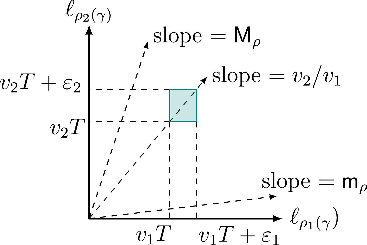


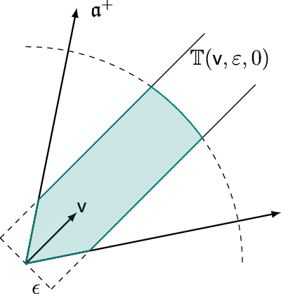
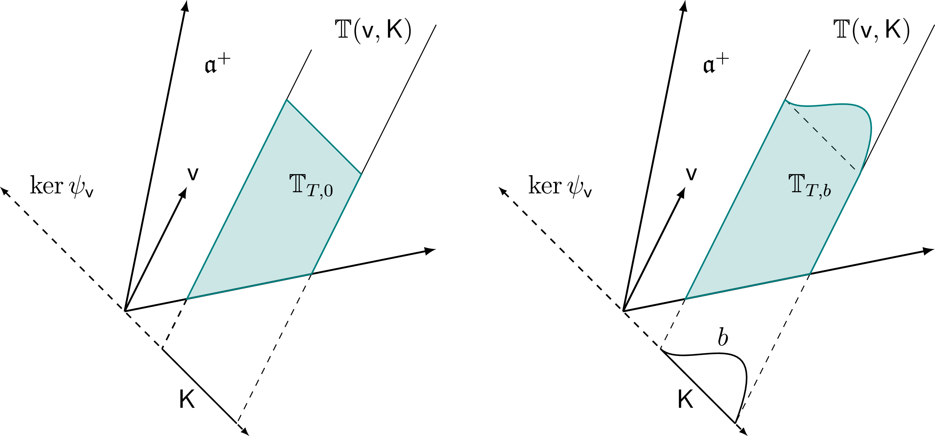
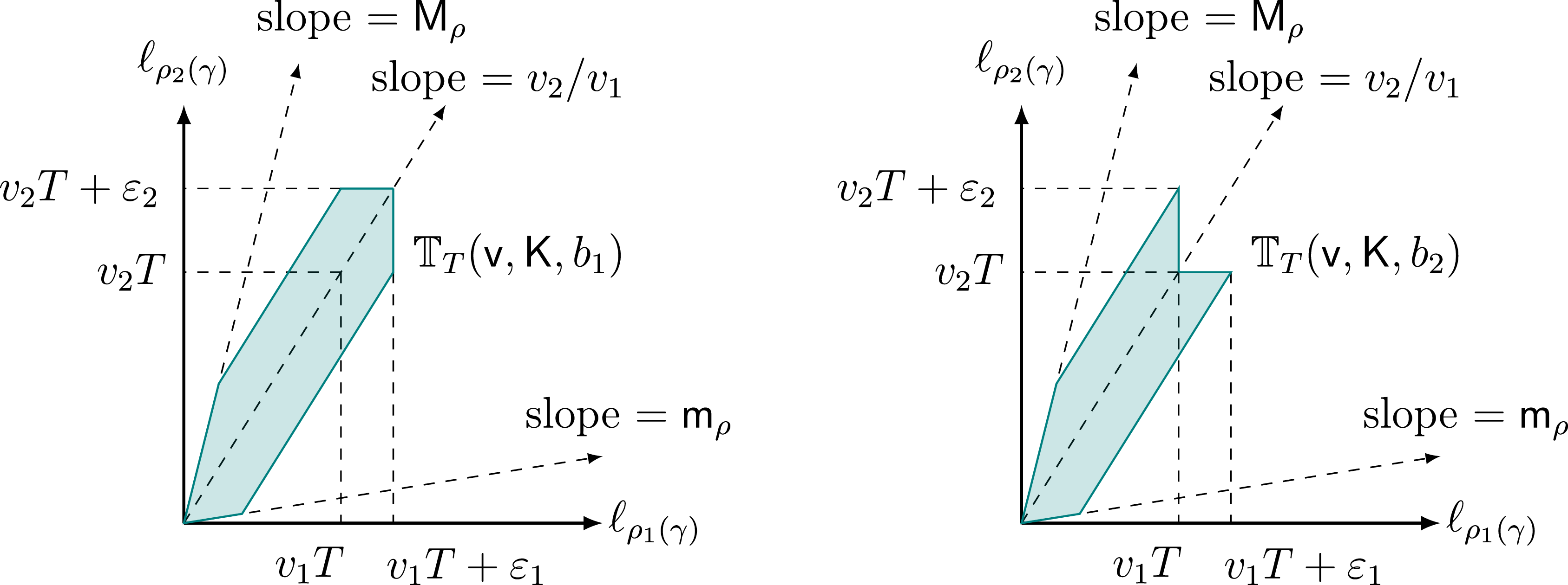

 Open access

