


1 Introduction
In various places around the world, severe forest fires have been observed to give rise to rotating columns of flame. In the most common instances, these are whipped up by local rotating winds, and so their formation is rather like that of a dust devil (or “willy-willy” in Australia). They are often referred to as fire whirls, fire tornadoes or even “firenadoes”. This terminology has been controversial (see McCarthy and Cormier [Reference McCarthy and Cormier17]), since a true tornado is a meteorological event in which a super-cell thunderstorm produces an intense rope-like vortex that descends to the ground, whereas fire whirls are generated at ground level. In any event, most fire whirls do not generate the enormous wind speeds created in tornadoes. It is possible to generate spectacular fire whirls safely in the laboratory, and an engaging example is given by Mészáros [Reference Mészáros18]. Experiments on a laboratory-scale fire vortex have also been carried out by Akhmetov et al. [Reference Akhmetov, Gavrilov and Nikulin3]. They compared measured speeds with some simple estimates and found reasonable agreement. An overview of fire whirls is given in the review article by Tohidi et al. [Reference Tohidi, Gollner and Xiao19].
Nevertheless, there are rare instances in which severe fires can generate rotating wind columns with speeds comparable to those in genuine tornadoes. Forthofer [Reference Forthofer9] gives a compelling and moving description of such an event; this was the Carr fire tornado that occurred in Northern California in July 2018. Forthofer estimated that wind speeds there were equivalent to those occurring in tornadoes of category 3 on the Fujita scale, and generated temperatures of about $1480^{\circ }$
C. Furthermore, by re-examining some historical fire-related tragedies, he concluded that the Hamburg firestorm in World War II and the 1923 firestorm that engulfed Tokyo after an earthquake may well have been examples of actual fire tornadoes. It is believed that a truly enormous fire can produce smoke and ash clouds several kilometres high; these also contain water vapour, perhaps from burnt vegetation, so that an ice-capped pyrocumulonimbus cloud forms at high altitude. The vorticity in this fire-generated thundercloud is then sufficient to create a tornado. The only fully documented case of such an event in the Southern Hemisphere appears to be the 2003 bushfire that devastated Australia’s capital city, Canberra. This is discussed in detail by Fromm et al. [Reference Fromm, Tupper, Rosenfeld, Servranckx and McRae10], who estimate that the pyrocumulonimbus cloud generated a tornado at category 2 on the Fujita scale. A photo of the event appears to show a funnel cloud, and there was a typical tornado damage track about 20 kilometres in length, accompanied by large black hailstones. The review article by Tomašević et al. [Reference Tomašević, Cheung, Vučetić and Fox-Hughes20] points out that several factors influence the likelihood of severe bushfire formation, but that these features that prevail in South-Eastern Australia (including Tasmania) also exist in the coastal regions of Croatia. A more recent article by Lareau et al. [Reference Lareau, Nauslar, Bentley, Roberts, Emmerson, Brong, Mehle and Wallman15] has analysed three tornadic firestorms in California, and found that, similar to the Canberra case, the data suggests category 2 tornadoes were formed, with pyrocumulonimbus clouds up to 16 kilometres high.
$1480^{\circ }$
C. Furthermore, by re-examining some historical fire-related tragedies, he concluded that the Hamburg firestorm in World War II and the 1923 firestorm that engulfed Tokyo after an earthquake may well have been examples of actual fire tornadoes. It is believed that a truly enormous fire can produce smoke and ash clouds several kilometres high; these also contain water vapour, perhaps from burnt vegetation, so that an ice-capped pyrocumulonimbus cloud forms at high altitude. The vorticity in this fire-generated thundercloud is then sufficient to create a tornado. The only fully documented case of such an event in the Southern Hemisphere appears to be the 2003 bushfire that devastated Australia’s capital city, Canberra. This is discussed in detail by Fromm et al. [Reference Fromm, Tupper, Rosenfeld, Servranckx and McRae10], who estimate that the pyrocumulonimbus cloud generated a tornado at category 2 on the Fujita scale. A photo of the event appears to show a funnel cloud, and there was a typical tornado damage track about 20 kilometres in length, accompanied by large black hailstones. The review article by Tomašević et al. [Reference Tomašević, Cheung, Vučetić and Fox-Hughes20] points out that several factors influence the likelihood of severe bushfire formation, but that these features that prevail in South-Eastern Australia (including Tasmania) also exist in the coastal regions of Croatia. A more recent article by Lareau et al. [Reference Lareau, Nauslar, Bentley, Roberts, Emmerson, Brong, Mehle and Wallman15] has analysed three tornadic firestorms in California, and found that, similar to the Canberra case, the data suggests category 2 tornadoes were formed, with pyrocumulonimbus clouds up to 16 kilometres high.
Mathematical modelling of fire whirls and fire tornadoes is clearly a difficult assignment, and much about these events is still unknown. The recent review article by Ahmad et al. [Reference Ahmad, Akafuah, Forthofer, Fuchihata, Hirasawa, Kuwana, Nakamura, Sekimoto, Saito and Williams2] gives an overview of modern efforts to understand fire whirls through the three-pronged approach of experimentation, theoretical analysis and computational mechanics. They suggest that there may not be a clear differentiation between large fire whirls and fire tornadoes, and that some of the earlier methods for distinguishing between the two may not be scientifically valid.
One of the earlier mathematical models for understanding the physical origins of fire whirls was published by Barcilon and Drazin [Reference Barcilon and Drazin5], who suggested that Rayleigh–Taylor and Kelvin–Helmholtz instabilities combine to produce highly unstable atmospheric flows. They did not explicitly consider the cylindrical shape of the fire whirl, but a slightly earlier article by Byram and Martin [Reference Byram and Martin6] carried out some experimental work, and used approximate momentum equations to estimate the shape of the rotating fire plume. They also suggested that accounting for condensing water vapour within the firenado could be important in modelling its energy and the height of the funnel cloud.
Computational fluid dynamics has been used by Cunningham and Reeder [Reference Cunningham and Reeder7] to model the 2003 fire tornado in Canberra. Their computer code assumed a three-dimensional compressible atmosphere, and evidently included a model of fluid turbulence. In addition, it accounted for atmospheric moisture and cloud formation. They report simulations that generated pyrocumulonimbus clouds and a tornadic vortex. Accounting for water vapour and condensation proved important in their model, which was able to generate conditions similar to those in the 2003 Canberra firenado. Grishin et al. [Reference Grishin, Matvienko and Rudi12] also carried out a computational solution for a fire whirl, and they give the details of their model. They solved the equations of viscous compressible fluid flow in axisymmetric geometry, with a k– $\epsilon $
model of turbulence. They did not account for the combustion chemistry or the presence of water vapour, and they concluded that the heat exchange between the fire and the air, and the presence of turbulence, were responsible for the formation of a heat tornado. In a later paper, Grishin and Matvienko [Reference Grishin and Matvienko11] used a finite-volume method to solve the axisymmetric, compressible, viscous fluid-flow equations, again with a k–
$\epsilon $
model of turbulence. They did not account for the combustion chemistry or the presence of water vapour, and they concluded that the heat exchange between the fire and the air, and the presence of turbulence, were responsible for the formation of a heat tornado. In a later paper, Grishin and Matvienko [Reference Grishin and Matvienko11] used a finite-volume method to solve the axisymmetric, compressible, viscous fluid-flow equations, again with a k– $\epsilon $
turbulence model, but now also including combustion chemistry with the species oxygen, nitrogen, carbon dioxide, carbon monoxide and water vapour taken into account in their model. They found that the rotational swirl speed had a strong effect on the height to which the thermal plume rises in the atmosphere.
$\epsilon $
turbulence model, but now also including combustion chemistry with the species oxygen, nitrogen, carbon dioxide, carbon monoxide and water vapour taken into account in their model. They found that the rotational swirl speed had a strong effect on the height to which the thermal plume rises in the atmosphere.
In the present paper, we investigate a model of the fire whirl that has been made to be as simple as possible. Axisymmetric equations for the plume shape are solved, as in the models of Grishin and colleagues [Reference Grishin and Matvienko11, Reference Grishin, Matvienko and Rudi12]. A simple Boussinesq approach to the fluid momentum equations is adopted, so that any possibility of an explicit interface at the edge of the fire plume is avoided. This allows us to obtain a rather complete linearized solution for the problem, apparently for the first time, and it provides valuable information about the flow within the firenado vortex. This is given in full in Section 3. We solve the nonlinear equations using a spectral method, which takes full advantage of the axisymmetric geometry through the use of the first-kind Bessel functions $J_0$
and
$J_0$
and $J_1$
as basis functions (see Abramowitz and Stegun [Reference Abramowitz and Stegun1, page 358]). As a result, numerical accuracy is greatly enhanced. The numerical scheme is outlined in Section 4 and some results are presented in Section 5. A surprising result is that large, energetic fires can be responsible for flow reversion within the rotating vortex, in which the tip points downward. This is discussed more fully in Section 6, where it is found that nonlinear convection effects can be responsible for a type of vortex breakdown at large fire amplitude
$J_1$
as basis functions (see Abramowitz and Stegun [Reference Abramowitz and Stegun1, page 358]). As a result, numerical accuracy is greatly enhanced. The numerical scheme is outlined in Section 4 and some results are presented in Section 5. A surprising result is that large, energetic fires can be responsible for flow reversion within the rotating vortex, in which the tip points downward. This is discussed more fully in Section 6, where it is found that nonlinear convection effects can be responsible for a type of vortex breakdown at large fire amplitude $\epsilon _F$
, through the formation of a stagnation streamsurface within the vortex, which separates a lower rotating cell from an upper counterrotating region. As time progresses, this upper region eventually dominates. Some further comments are given in the concluding Section 7.
$\epsilon _F$
, through the formation of a stagnation streamsurface within the vortex, which separates a lower rotating cell from an upper counterrotating region. As time progresses, this upper region eventually dominates. Some further comments are given in the concluding Section 7.
2 The mathematical model
This simple idealization of a rotating firestorm event assumes that there is some (circular) patch of burning (homogeneous) grassland, of radius a. The ground is taken to be the plane $z=0$
in a Cartesian coordinate system in which the z-axis points vertically, and the origin is located at the centre of the circular combustion region. The air is modelled here as a weakly compressible fluid of density
$z=0$
in a Cartesian coordinate system in which the z-axis points vertically, and the origin is located at the centre of the circular combustion region. The air is modelled here as a weakly compressible fluid of density $\rho $
, that is subject to the downward acceleration
$\rho $
, that is subject to the downward acceleration $-g \mathbf {e_z}$
of gravity.
$-g \mathbf {e_z}$
of gravity.
In reality, the burning process occurring within the disk $r<a$
of bushland, near ground level, would involve a sequence of combustion reactions, as well as the production of flammable gases, perhaps similar to the processes described by Forbes [Reference Forbes8] in his model of an Australian bushfire. Here, however, all that is ignored, and it is assumed instead that the burning reactions effectively result in an elevated ground-level temperature
$r<a$
of bushland, near ground level, would involve a sequence of combustion reactions, as well as the production of flammable gases, perhaps similar to the processes described by Forbes [Reference Forbes8] in his model of an Australian bushfire. Here, however, all that is ignored, and it is assumed instead that the burning reactions effectively result in an elevated ground-level temperature
 $$ \begin{align} T(r,0,t) = T_a + ( T_F - T_a ) f(r)\quad \text{on } z=0 , \end{align} $$
in which the ambient temperature is $T_a$
and the temperature at the centre of the fire is
$T_a$
and the temperature at the centre of the fire is $T_F$
. The dimensionless shape function
$T_F$
. The dimensionless shape function $f(r)$
gives the ground-level temperature profile; at the centre
$f(r)$
gives the ground-level temperature profile; at the centre $r=0$
it follows that
$r=0$
it follows that $f(0)=1$
, and far away the temperature falls back to ambient, so that
$f(0)=1$
, and far away the temperature falls back to ambient, so that $f ( \infty ) = 0$
.
$f ( \infty ) = 0$
.
To simplify the model, we now make use of the Boussinesq approximation (see Vallis [Reference Vallis21, Section 2.4]). This essentially postulates a linear variation of the air temperature T with its density $\rho $
, which can be understood to be the first-order term in a Taylor series of some more complicated function
$\rho $
, which can be understood to be the first-order term in a Taylor series of some more complicated function $T(\rho )$
about the ambient density
$T(\rho )$
about the ambient density $\rho _a$
. Boussinesq theory makes the approximation
$\rho _a$
. Boussinesq theory makes the approximation
 $$ \begin{align} \rho = \rho_a + \overline{\rho}, \end{align} $$
in which the correction function $\overline {\rho }$
is small relative to
$\overline {\rho }$
is small relative to $\rho _a$
. This is related to the temperature by the linearized condition
$\rho _a$
. This is related to the temperature by the linearized condition
 $$ \begin{align} \overline{\rho} = - A_T \rho_a ( T - T_a ). \end{align} $$
A negative sign is present to emphasize the fact that air density decreases with increasing temperature, and the positive constant $A_T$
is the coefficient of thermal expansion of the air.
$A_T$
is the coefficient of thermal expansion of the air.
Cylindrical polar coordinates $( r, \theta , z )$
will be used in this analysis, since a cylindrical “firenado” will be assumed here, as a further simplification. These are related to the usual Cartesian coordinates
$( r, \theta , z )$
will be used in this analysis, since a cylindrical “firenado” will be assumed here, as a further simplification. These are related to the usual Cartesian coordinates $( x,y,z )$
by the familiar formulae
$( x,y,z )$
by the familiar formulae $x = r \cos \theta $
and
$x = r \cos \theta $
and $y = r\sin \theta $
. In cylindrical coordinates, the velocity vector
$y = r\sin \theta $
. In cylindrical coordinates, the velocity vector $\mathbf {q}$
of the air is represented in component form as
$\mathbf {q}$
of the air is represented in component form as
 $$ \begin{align} \mathbf{q} = u \mathbf{e_r} + v \mathbf{e}_{\boldsymbol{\theta}} + w \mathbf{e_z}. \end{align} $$
In Boussinesq theory, the exact continuity equation expressing the conservation of mass in a compressible gas is further “split” into an incompressible equation
 $$ \begin{align} \boldsymbol{\nabla} \centerdot \mathbf{q} = 0, \end{align} $$
and a remnant transport equation for the density correction term $\overline {\rho }$
that is convected about in the fluid. Equivalently, in view of the relation (2.3), the temperature obeys an energy-conservation law of the form
$\overline {\rho }$
that is convected about in the fluid. Equivalently, in view of the relation (2.3), the temperature obeys an energy-conservation law of the form
 $$ \begin{align} \frac {\partial T}{\partial t} + \mathbf{q} \centerdot \boldsymbol{\nabla} T = B \nabla^2 T - h ( T - T_a ). \end{align} $$
Here, the constant B is a diffusion coefficient for temperature, and h represents the coefficient of Newtonian cooling of the air to the ambient temperature $T_a$
. Newton’s law of cooling is an approximation that assumes convective heat transfer, in which the coefficient h is constant. Further details are given in a recent e-book by Lienhard and Lienhard [Reference Lienhard and Lienhard16, page 19]. (Here, we do not consider radiation effects, which are modelled using Stefan’s law [Reference Lienhard and Lienhard16, page 71].)
$T_a$
. Newton’s law of cooling is an approximation that assumes convective heat transfer, in which the coefficient h is constant. Further details are given in a recent e-book by Lienhard and Lienhard [Reference Lienhard and Lienhard16, page 19]. (Here, we do not consider radiation effects, which are modelled using Stefan’s law [Reference Lienhard and Lienhard16, page 71].)
Conservation of momentum within the moving air is modelled using the familiar Navier–Stokes equation; however, in the Boussinesq approximation, the exact density term (2.2) is retained only where it multiplies the acceleration g of gravity in the buoyancy term. This results in the Navier–Stokes–Boussinesq equation
 $$ \begin{align} \rho_a \bigg[ \frac{\partial \mathbf{q}}{\partial t} + ( \mathbf{q} \centerdot \boldsymbol{\nabla} ) \mathbf{q} \bigg] + \boldsymbol{\nabla} p = - ( \rho_a + \rho ) g \mathbf{e_z} + \mu \nabla^2 \mathbf{q} , \end{align} $$
in which the function p denotes the pressure in the air. The kinematic viscosity is $\mu $
, and in the vortex, where the flow is possibly turbulent,
$\mu $
, and in the vortex, where the flow is possibly turbulent, $\mu $
would represent an effective turbulent viscosity. Boundary layers are ignored here for simplicity, so that the air effectively slips over the ground plane
$\mu $
would represent an effective turbulent viscosity. Boundary layers are ignored here for simplicity, so that the air effectively slips over the ground plane $z=0$
.
$z=0$
.
Nondimensional coordinates are now introduced, since this reduces the number of free constants in the model, and can assist in elucidating the mathematical structure of closed-form solutions, such as that discussed in Section 3. Lengths are all scaled relative to the notional ground radius a of the circular fire column. Time and speeds are scaled using the quantities $\sqrt {a/g}$
and
$\sqrt {a/g}$
and $\sqrt {ag}$
, in which g is the downward acceleration of gravity. The (ambient) temperature
$\sqrt {ag}$
, in which g is the downward acceleration of gravity. The (ambient) temperature $T_a$
and density
$T_a$
and density $\rho _a$
far away are used as reference values for temperature and density throughout the atmosphere, so that
$\rho _a$
far away are used as reference values for temperature and density throughout the atmosphere, so that $a g \rho _a$
is the natural reference scale for pressure. A sketch of the dimensionless coordinate system is given in Figure 1. In this dimensionless formulation, solutions are thus found to depend upon five nondimensional parameters. These are
$a g \rho _a$
is the natural reference scale for pressure. A sketch of the dimensionless coordinate system is given in Figure 1. In this dimensionless formulation, solutions are thus found to depend upon five nondimensional parameters. These are
 $$ \begin{align} \begin{aligned} \alpha &= A_T T_a ,\quad \beta = \frac{B}{\sqrt{a^3 g}} ,\quad \frac{1}{R_e} = \frac{\mu}{\rho_a \sqrt{a^3 g}},\\ \chi_N &= h \sqrt{\frac{a}{g}}, \quad \epsilon_F = \frac{T_F - T_a}{T_a}. \end{aligned} \end{align} $$
The first parameter $\alpha $
is the dimensionless thermal-expansion coefficient in the atmosphere, and
$\alpha $
is the dimensionless thermal-expansion coefficient in the atmosphere, and $\beta $
is the coefficient of thermal diffusion. The Reynolds number
$\beta $
is the coefficient of thermal diffusion. The Reynolds number $R_e$
is essentially a measure of the inverse viscosity, so that, if
$R_e$
is essentially a measure of the inverse viscosity, so that, if $R_e$
is small then the fluid is very viscous, whereas the effects of viscosity become negligible as
$R_e$
is small then the fluid is very viscous, whereas the effects of viscosity become negligible as $R_e \rightarrow \infty $
. The parameter
$R_e \rightarrow \infty $
. The parameter $\chi _N$
represents the rate of Newtonian cooling of the atmosphere, and
$\chi _N$
represents the rate of Newtonian cooling of the atmosphere, and $\epsilon _F$
gives the temperature rise within the “firenado” relative to the ambient temperature. There may also be extra parameters associated with the function
$\epsilon _F$
gives the temperature rise within the “firenado” relative to the ambient temperature. There may also be extra parameters associated with the function $f(r)$
in the boundary condition (2.1) for the temperature at ground level.
$f(r)$
in the boundary condition (2.1) for the temperature at ground level.
Dimensionless coordinate system used for the firenado model. The central disk of radius $r=1$
represents the location of the swirling fire. In the linearized solution of Section 3 the fluid domain is the entire half-space
$r=1$
represents the location of the swirling fire. In the linearized solution of Section 3 the fluid domain is the entire half-space $z>0$
, but in the nonlinear spectral solution in Section 4 the computational domain is restricted to
$z>0$
, but in the nonlinear spectral solution in Section 4 the computational domain is restricted to $0 < r < R_{\infty }$
,
$0 < r < R_{\infty }$
, $0 < z < Z_{\infty }$
as shown.
$0 < z < Z_{\infty }$
as shown.

In cylindrical polar coordinates and in these dimensionless variables, the incompressibility condition (2.5) takes the form
 $$ \begin{align} \frac{1}{r} \frac{\partial}{\partial r} ( r u ) + \frac{\partial w}{\partial z} = 0. \end{align} $$
The relationship (2.3) between the air temperature and the density becomes
 $$ \begin{align} \overline{\rho} = - \alpha ( T - 1 ). \end{align} $$
The three components of the momentum equation (2.7) in the r- , $\theta $
- and z-directions, respectively, are
$\theta $
- and z-directions, respectively, are
 $$ \begin{align} \frac{\partial u}{\partial t} + u \frac{\partial u}{\partial r} + w \frac{\partial u}{\partial z} - \frac{v^2}{r} + \frac{\partial p}{\partial r} & = \frac{1}{R_e} \bigg[ \nabla^2 u - \frac{u}{r^2} \bigg], \nonumber \\ \frac{\partial v}{\partial t} + u \frac{\partial v}{\partial r} + w \frac{\partial v}{\partial z} + \frac{u v}{r} & = \frac{1}{R_e} \bigg[ \nabla^2 v - \frac{v}{r^2} \bigg], \\ \frac{\partial w}{\partial t} + u \frac{\partial w}{\partial r} + w \frac{\partial w}{\partial z} + \frac{\partial p}{\partial z} & = - ( 1 + \overline{\rho} ) + \frac{1}{R_e} \nabla^2 w. \nonumber \end{align} $$
Finally, the convective heat equation (2.6) takes the form
 $$ \begin{align} \frac {\partial T}{\partial t} + u \frac{\partial T}{\partial r} + w \frac{\partial T}{\partial z} = \beta \nabla^2 T - \chi_N ( T - 1 ). \end{align} $$
In these relations (2.11) and (2.12), the operator
 $$ \begin{align} \nabla^2 T = \frac{1}{r} \frac{\partial}{\partial r} \bigg( r \frac{\partial T}{\partial r} \bigg) + \frac{\partial^2 T}{\partial z^2}, \end{align} $$
acting here on a function $T (r,z,t)$
, is the Laplacian derivative in cylindrical polar coordinates, in the axisymmetric case for which
$T (r,z,t)$
, is the Laplacian derivative in cylindrical polar coordinates, in the axisymmetric case for which $\partial / \partial \theta \equiv 0$
. As discussed above, the effect of the burning vegetation is modelled here very simply by imposing an effective temperature (2.1) at ground level. In dimensionless coordinates, we generalize the boundary condition (2.1) slightly, by multiplying the perturbation temperature by a smoothly increasing function of time. We choose a relation of the form
$\partial / \partial \theta \equiv 0$
. As discussed above, the effect of the burning vegetation is modelled here very simply by imposing an effective temperature (2.1) at ground level. In dimensionless coordinates, we generalize the boundary condition (2.1) slightly, by multiplying the perturbation temperature by a smoothly increasing function of time. We choose a relation of the form
 $$ \begin{align} T(r,0,t) = 1 + \epsilon_F f(r) \bigg[ 1 - \exp \bigg( - \frac{t}{\tau_F} \bigg) \bigg] \quad \text{on } z=0, \end{align} $$
since this allows a smooth increase in temperature T from the ambient value $T=1$
at
$T=1$
at $t=0$
to the final value
$t=0$
to the final value $T = 1 + \epsilon _F f(r)$
, without the discontinuity indicated in (2.1). This boundary condition (2.14) does, however, involve an additional dimensionless time constant
$T = 1 + \epsilon _F f(r)$
, without the discontinuity indicated in (2.1). This boundary condition (2.14) does, however, involve an additional dimensionless time constant $\tau _F$
. Notice that a swirling component
$\tau _F$
. Notice that a swirling component $v (r,z,t)$
of the velocity vector
$v (r,z,t)$
of the velocity vector $\mathbf {q}$
is still retained in the momentum equations (2.11), even although dependence on the azimuthal coordinate
$\mathbf {q}$
is still retained in the momentum equations (2.11), even although dependence on the azimuthal coordinate $\theta $
is ignored.
$\theta $
is ignored.
3 A linearized solution
In this section, an approximate theory is derived, in which the temperature inside the “firenado” is assumed not to be very much greater than the ambient temperature. This means that the parameter $\epsilon _F$
in (2.8) is small. Consequently, we express the solution variables in perturbation expansions about the ambient conditions, and postulate
$\epsilon _F$
in (2.8) is small. Consequently, we express the solution variables in perturbation expansions about the ambient conditions, and postulate
 $$ \begin{align} T(r,z,t) & = 1 + \epsilon_F T^L (r,z,t) + \mathcal{O} ( \epsilon_F^2 ), \nonumber \\ u(r,z,t) & = \quad\quad \epsilon_F U^L (r,z,t) + \mathcal{O} ( \epsilon_F^2 ), \nonumber \\ v(r,z,t) & = \quad\quad \epsilon_F V^L (r,z,t) + \mathcal{O} ( \epsilon_F^2 ), \\ w(r,z,t) & = \quad\quad \epsilon_F W^L (r,z,t) + \mathcal{O} ( \epsilon_F^2 ), \nonumber \\ \overline{\rho}(r,z,t) & = \quad\quad \epsilon_F \rho^L (r,z,t) + \mathcal{O} ( \epsilon_F^2 ), \nonumber \\ p(r,z,t) & = - z + \epsilon_F p^L (r,z,t) + \mathcal{O} (\epsilon_F^2). \nonumber \end{align} $$
These forms of the solution variables are substituted into the governing equations (2.9)–(2.12), and terms are retained to the first order in the small parameter $\epsilon _F$
. This gives rise to a linear set of partial differential equations for the approximate solution variables
$\epsilon _F$
. This gives rise to a linear set of partial differential equations for the approximate solution variables $T^L$
and so on.
$T^L$
and so on.
The linearized approximation to the continuity equation (2.9) is readily seen to be
 $$ \begin{align} \frac{1}{r} \frac{\partial}{\partial r} ( r U^L ) + \frac{\partial W^L}{\partial z} = 0, \end{align} $$
and the Boussinesq equation of state (2.10) becomes simply
 $$ \begin{align} \rho^L = - \alpha T^L \end{align} $$
in the linear approximation. At the first order in $\epsilon _F$
the three components of the momentum equation (2.11) reduce to
$\epsilon _F$
the three components of the momentum equation (2.11) reduce to
 $$ \begin{align} \frac{\partial U^L}{\partial t} + \frac{\partial p^L}{\partial r} & = \frac{1}{R_e} \bigg[ \nabla^2 U^L - \frac{U^L}{r^2} \bigg], \nonumber \\ \frac{\partial V^L}{\partial t} & = \frac{1}{R_e} \bigg[ \nabla^2 V^L - \frac{V^L}{r^2} \bigg], \\ \frac{\partial W^L}{\partial t} + \frac{\partial p^L}{\partial z} & = - \rho^L + \frac{1}{R_e} \nabla^2 W^L, \nonumber \end{align} $$
in which $\nabla ^2$
is the scalar operator given in (2.13). The linearized form of the energy equation (2.12) is
$\nabla ^2$
is the scalar operator given in (2.13). The linearized form of the energy equation (2.12) is
 $$ \begin{align} \frac {\partial T^L}{\partial t} = \beta \nabla^2 T^L - \chi_N T^L. \end{align} $$
In this linearized approximation, the heat law (3.5) decouples from the rest of the equations in the system, and so can be solved separately, subject to the boundary condition
 $$ \begin{align} T^L (r,0,t) = f(r) \bigg[ 1 - \exp \bigg( - \frac{t}{\tau_F} \bigg) \bigg] \quad \text{on } z=0. \end{align} $$
These equations can be solved using Hankel and Laplace transforms [Reference Abramowitz and Stegun1] over the semi-infinite domain $0 < r < \infty $
,
$0 < r < \infty $
, $0 < z < \infty $
, but the result is sufficiently complicated as to be somewhat unenlightening. Consequently, we choose instead to solve over the approximate computational region
$0 < z < \infty $
, but the result is sufficiently complicated as to be somewhat unenlightening. Consequently, we choose instead to solve over the approximate computational region $0 < r < R_{\infty }$
,
$0 < r < R_{\infty }$
, $0 < z < Z_{\infty }$
illustrated in Figure 1. The appropriate additional boundary conditions in this case are
$0 < z < Z_{\infty }$
illustrated in Figure 1. The appropriate additional boundary conditions in this case are $T^L = 0$
on
$T^L = 0$
on $r = R_{\infty }$
and
$r = R_{\infty }$
and $T^L = 0$
on
$T^L = 0$
on $z = Z_{\infty }$
.
$z = Z_{\infty }$
.
After a little trial and error, it becomes evident that a pragmatic form for the linearized temperature function $T^L$
is
$T^L$
is
 $$ \begin{align} T^L (r,z,t) & = \cos \bigg( \frac{\pi z}{2 Z_{\infty}} \bigg) \sum_{m=1}^{\infty} A_{m,0}(t) J_0 ( p_m r )\nonumber \\ & \quad + \sum_{m=1}^{\infty} \sum_{n=1}^{\infty} A_{m,n}(t) J_0 ( p_m r ) \sin \bigg( \frac{n \pi z}{Z_{\infty}} \bigg), \end{align} $$
in which the eigenvalues $p_m$
are given by
$p_m$
are given by
 $$ \begin{align} p_m = j_{0,m} / R_{\infty}. \end{align} $$
The function $J_0 (z)$
is the zeroth-order Bessel function of the first kind, and
$J_0 (z)$
is the zeroth-order Bessel function of the first kind, and $j_{0,m}$
,
$j_{0,m}$
, $m = 1, 2, 3, \ldots ,$
are its zeros (see Abramowitz and Stegun [Reference Abramowitz and Stegun1, Ch. 9]), so that
$m = 1, 2, 3, \ldots ,$
are its zeros (see Abramowitz and Stegun [Reference Abramowitz and Stegun1, Ch. 9]), so that ${J_0 ( j_{0,m} ) = 0}$
. This satisfies the condition
${J_0 ( j_{0,m} ) = 0}$
. This satisfies the condition $T^L = 0$
on the artificial computational boundaries shown in Figure 1. The bottom boundary condition (3.6) on
$T^L = 0$
on the artificial computational boundaries shown in Figure 1. The bottom boundary condition (3.6) on $z=0$
, combined with the form (3.7) of the solution, gives rise to the requirement
$z=0$
, combined with the form (3.7) of the solution, gives rise to the requirement
 $$ \begin{align*} f(r) \bigg[ 1 - \exp \bigg( - \frac{t}{\tau_F} \bigg) \bigg] = \sum_{m=1}^{\infty} A_{m,0}(t) J_0 ( p_m r ). \end{align*} $$
This condition is multiplied by basis functions $r J_0 ( p_k r )$
,
$r J_0 ( p_k r )$
, $k = 1,2, 3, \ldots ,$
and integrated over the domain
$k = 1,2, 3, \ldots ,$
and integrated over the domain $0< r < R_{\infty }$
. The orthogonality of the Bessel functions then gives the coefficients for
$0< r < R_{\infty }$
. The orthogonality of the Bessel functions then gives the coefficients for $n=0$
in the form
$n=0$
in the form
 $$ \begin{align} A_{k,0}(t) = \frac{1}{\Lambda_k} \bigg[ 1 - \exp \bigg( - \frac{t}{\tau_F} \bigg) \bigg] \int_0^{R_{\infty}} r f(r) J_0 ( p_k r ) \, \textit{d} r, \end{align} $$
in which we have defined constants
 $$ \begin{align} \Lambda_k = \tfrac{1}{2} [ R_{\infty} J_1 ( p_k R_{\infty} ) ]^2. \end{align} $$
Here, $J_1$
is the first-kind Bessel function of order
$J_1$
is the first-kind Bessel function of order $1$
.
$1$
.
The form (3.7) is next substituted into the linearized energy equation (3.5), to determine the remaining coefficient functions $A_{m,n}(t)$
. This gives
$A_{m,n}(t)$
. This gives
 $$ \begin{align*} \cos &\bigg( \frac{\pi z}{2 Z_{\infty}} \bigg) \sum_{m=1}^{\infty} \frac{\textit{d} A_{m,0}(t)}{\textit{d} t} J_0 ( p_m r ) + \sum_{m=1}^{\infty} \sum_{n=1}^{\infty} \frac{\textit{d} A_{m,n}(t)}{\textit{d} t} J_0 ( p_m r ) \sin \bigg( \frac{n \pi z}{Z_{\infty}} \bigg) \nonumber \\ & = - \cos \bigg( \frac{\pi z}{2 Z_{\infty}} \bigg) \sum_{m=1}^{\infty} A_{m,0}(t) \Gamma_m J_0 ( p_m r ) - \sum_{m=1}^{\infty} \sum_{n=1}^{\infty} A_{m,n}(t) \Delta_{m,n} J_0 ( p_m r ) \sin \bigg( \frac{n \pi z}{Z_{\infty}} \bigg). \nonumber \end{align*} $$
This equation is multiplied by $r J_0 ( p_k r ) \sin ( \ell \pi z / Z_{\infty } )$
,
$r J_0 ( p_k r ) \sin ( \ell \pi z / Z_{\infty } )$
, $k = 1,2, \ldots ,$
and integrated over the computational domain
$k = 1,2, \ldots ,$
and integrated over the computational domain $0 < r < R_{\infty }$
,
$0 < r < R_{\infty }$
, $0 < z < Z_{\infty }$
. After some algebra, this results in the infinite system of ordinary differential equations
$0 < z < Z_{\infty }$
. After some algebra, this results in the infinite system of ordinary differential equations
 $$ \begin{align} \frac{\textit{d} A_{k,\ell}(t)}{\textit{d} t} + \Delta_{k,\ell} A_{k,\ell}(t) & = - \frac{8\ell}{\pi ( 2\ell - 1 ) ( 2\ell + 1 )} \bigg[\frac{\textit{d} A_{k,0}(t)}{\textit{d} t} + \Gamma_{k} A_{k,0}(t) \bigg],\nonumber \\ & \quad k = 1, 2, \ldots, \quad \ell = 1, 2, \ldots. \end{align} $$
In obtaining these equations, the following integral was used:
 $$ \begin{align} \int_0^{Z_{\infty}} \cos \bigg( \frac{\pi z}{2 Z_{\infty}} \bigg) \sin \bigg( \frac{\ell \pi z}{Z_{\infty}} \bigg) \, \textit{d} z = \frac{4 \ell Z_{\infty}}{\pi ( 2\ell - 1 ) ( 2\ell + 1 )}. \end{align} $$
In these expressions, we have defined additional constants
 $$ \begin{align} \begin{aligned} \Gamma_{k} & = \beta \bigg[ p_k^2 + \bigg(\frac{\pi}{2 Z_{\infty}}\bigg)^2 \bigg] + \chi_N , \\ \Delta_{k,\ell} & = \beta \bigg[ p_k^2 + \bigg(\frac{\ell \pi}{Z_{\infty}} \bigg)^2 \bigg] + \chi_N. \end{aligned} \end{align} $$
The zeroth-order coefficients $A_{k,0}(t)$
are known exactly from (3.9), so that the terms on the right of (3.11) can be evaluated. The initial condition
$A_{k,0}(t)$
are known exactly from (3.9), so that the terms on the right of (3.11) can be evaluated. The initial condition $T^L = 0$
when
$T^L = 0$
when $t=0$
then means that each differential equation in (3.11) is solved subject to
$t=0$
then means that each differential equation in (3.11) is solved subject to $A_{k,\ell }(0) = 0$
. The result is
$A_{k,\ell }(0) = 0$
. The result is
 $$ \begin{align} A_{k,\ell}(t) & = \mathcal{C}_{k,\ell}^A \bigg\{\frac{\Gamma_k}{\Delta_{k,l}} [ \exp ( - \Delta_{k,\ell} t ) - 1 ] \nonumber \\ & \quad + \frac{ ( 1 - \tau_F \Gamma_k )}{( \tau_F \Delta_{k,\ell} - 1 )} [ \exp ( - \Delta_{k,\ell} t ) - \exp ( - t / \tau_F ) ] \bigg\}, \end{align} $$
where we have defined
 $$ \begin{align} \mathcal{C}_{k,\ell}^A = \frac{8 \ell}{\Lambda_k \pi ( 2\ell - 1 ) ( 2\ell + 1 )} \int_0^{R_{\infty}} r f(r) J_0 ( p_k r ) \, \textit{d} r, \end{align} $$
and the constants defined in (3.10) and (3.13) have also been utilized. Thus the complete solution for the temperature perturbation function $T^L$
in the linearized approximation is given by (3.7) with (3.9) and (3.14). The density perturbation function
$T^L$
in the linearized approximation is given by (3.7) with (3.9) and (3.14). The density perturbation function $\rho ^L$
is then found at once from (3.3).
$\rho ^L$
is then found at once from (3.3).
The linearized swirl component $V_L$
of velocity satisfies the azimuthal component of the momentum equation in (3.4). This must be solved subject to specifying the azimuthal velocity at ground level, and following the formulation developed in (3.6), we give the function
$V_L$
of velocity satisfies the azimuthal component of the momentum equation in (3.4). This must be solved subject to specifying the azimuthal velocity at ground level, and following the formulation developed in (3.6), we give the function
 $$ \begin{align} V^L (r,0,t) = h(r) \bigg[ 1 - \exp \bigg( - \frac{t}{\tau_F} \bigg) \bigg] \quad \text{on } z=0. \end{align} $$
It is appropriate again to allow the swirl velocity component to have a similar type of structure to that used for the temperature perturbation function $T^L$
in (3.7), and so here we choose
$T^L$
in (3.7), and so here we choose
 $$ \begin{align} V^L (r,z,t) & = \cos \bigg( \frac{\pi z}{2 Z_{\infty}} \bigg) \sum_{m=1}^{\infty} B_{m,0}(t) J_1 ( p_m r ) \nonumber \\ & \quad + \sum_{m=1}^{\infty} \sum_{n=1}^{\infty} B_{m,n}(t) J_1 ( p_m r ) \sin \bigg( \frac{n \pi z}{Z_{\infty}} \bigg), \end{align} $$
with constants $p_m$
given in (3.8), as before. Notice, however, that the first-order Bessel function
$p_m$
given in (3.8), as before. Notice, however, that the first-order Bessel function $J_1$
is used in (3.17) since we require
$J_1$
is used in (3.17) since we require $V^L = 0$
on the z-axis
$V^L = 0$
on the z-axis $r=0$
.
$r=0$
.
Applying the ground-level boundary condition (3.16) leads at once to the equation
 $$ \begin{align*} h(r) \bigg[ 1 - \exp \bigg( - \frac{t}{\tau_F} \bigg) \bigg] = \sum_{m=1}^{\infty} B_{m,0}(t) J_1 ( p_m r ). \end{align*} $$
This is then multiplied by basis functions $r J_1 ( p_k r )$
,
$r J_1 ( p_k r )$
, $k = 1,2, 3, \ldots ,$
and integrated over the domain
$k = 1,2, 3, \ldots ,$
and integrated over the domain $0< r < R_{\infty }$
, following the same development as in (3.9) above. The first-order Bessel functions
$0< r < R_{\infty }$
, following the same development as in (3.9) above. The first-order Bessel functions $J_1$
satisfy the same orthogonality conditions, and so the coefficients for the rotational speed at zeroth order
$J_1$
satisfy the same orthogonality conditions, and so the coefficients for the rotational speed at zeroth order $n=0$
are similarly found to be
$n=0$
are similarly found to be
 $$ \begin{align} B_{k,0}(t) = \frac{1}{\Lambda_k} \bigg[ 1 - \exp \bigg( - \frac{t}{\tau_F} \bigg) \bigg] \int_0^{R_{\infty}} r h(r) J_1 ( p_k r ) \, \textit{d} r. \end{align} $$
The constants $\Lambda _k$
are those defined in (3.10).
$\Lambda _k$
are those defined in (3.10).
The remaining coefficients in the form (3.17) are found by substituting this expression into the linearized azimuthal component of the momentum equation (3.4). This is then multiplied by $r J_1 ( p_k r ) \sin ( \ell \pi z / Z_{\infty } )$
,
$r J_1 ( p_k r ) \sin ( \ell \pi z / Z_{\infty } )$
, $k = 1,2, \ldots ,$
and integrated over the computational domain
$k = 1,2, \ldots ,$
and integrated over the computational domain $0 < r < R_{\infty }$
,
$0 < r < R_{\infty }$
, $0 < z < Z_{\infty }$
. The calculations are similar to those leading to the differential equations (3.11), and a significant amount of algebra gives rise to the system
$0 < z < Z_{\infty }$
. The calculations are similar to those leading to the differential equations (3.11), and a significant amount of algebra gives rise to the system
 $$ \begin{align} \frac{\textit{d} B_{k,\ell}(t)}{\textit{d} t} + \delta_{k,\ell} B_{k,\ell}(t) & = - \frac{8\ell}{\pi ( 2\ell - 1 ) ( 2\ell + 1 )} \bigg[\frac{\textit{d} B_{k,0}(t)}{\textit{d} t} + \gamma_{k} B_{k,0}(t) \bigg], \nonumber \\ & \quad k = 1, 2, \ldots, \quad \ell = 1, 2, \ldots, \end{align} $$
in which we have defined further auxiliary constants
 $$ \begin{align} \begin{aligned}\gamma_{k} & = \frac{1}{R_e} \bigg[ p_k^2 + \bigg( \frac{\pi}{2 Z_{\infty}} \bigg)^2 \bigg], \\ \delta_{k,\ell} & = \frac{1}{R_e} \bigg[ p_k^2 + \bigg( \frac{\ell \pi}{Z_{\infty}} \bigg)^2 \bigg]. \end{aligned}\end{align} $$
Here, we have again made use of the integral (3.12). The differential equations in (3.19) are solved subject to the initial conditions $B_{k,\ell } (0) = 0$
to give
$B_{k,\ell } (0) = 0$
to give
 $$ \begin{align} B_{k,\ell}(t) & = \mathcal{C}_{k,\ell}^B \bigg\{ \frac{\gamma_k}{\delta_{k,l}} [ \exp ( - \delta_{k,\ell} t ) - 1 ] \nonumber \\ &\quad + \frac{ ( 1 - \tau_F \gamma_k )}{( \tau_F \delta_{k,\ell} - 1 )} [ \exp ( - \delta_{k,\ell} t ) - \exp ( - t / \tau_F ) ] \bigg\}. \end{align} $$
In this expression, we have defined
 $$ \begin{align} \mathcal{C}_{k,\ell}^B = \frac{8 \ell}{\Lambda_k \pi ( 2\ell - 1 ) ( 2\ell + 1 )} \int_0^{R_{\infty}} r h(r) J_1 ( p_k r ) \, \textit{d} r, \end{align} $$
and the constants $\gamma _k$
and
$\gamma _k$
and $\delta _{k,\ell }$
are as defined in (3.20).
$\delta _{k,\ell }$
are as defined in (3.20).
Finally, it is required to calculate linearized velocity components $U^L$
and
$U^L$
and $W^L$
in the radial and vertical directions so as to satisfy the (linearized) incompressibility condition (3.2). We do this by making use of an axisymmetric streamfunction
$W^L$
in the radial and vertical directions so as to satisfy the (linearized) incompressibility condition (3.2). We do this by making use of an axisymmetric streamfunction $\Psi ^L (r,z,t)$
. The linearized velocity vector is expressed as
$\Psi ^L (r,z,t)$
. The linearized velocity vector is expressed as $\mathbf {q}^L = \mathrm {curl} ( \Psi ^L \mathbf {e}_{\boldsymbol {\theta }} ) + V^L \mathbf {e}_{\boldsymbol {\theta }}$
so that (3.2) is satisfied identically by means of the relations
$\mathbf {q}^L = \mathrm {curl} ( \Psi ^L \mathbf {e}_{\boldsymbol {\theta }} ) + V^L \mathbf {e}_{\boldsymbol {\theta }}$
so that (3.2) is satisfied identically by means of the relations
 $$ \begin{align} U^L (r,z,t) = - \frac{\partial \Psi^L}{\partial z}, \quad W^L (r,z,t) = \frac{1}{r} \frac{\partial}{\partial r} ( r \Psi^L ). \end{align} $$
For simplicity, we choose to ignore the narrow boundary layer near the ground, and so allow horizontal slip at the plane $z=0$
. Nevertheless, there is no vertical velocity component there, so that the boundary condition
$z=0$
. Nevertheless, there is no vertical velocity component there, so that the boundary condition $W^L (r,0,t) = 0$
applies. In addition, no radial outflow can occur on the z-axis
$W^L (r,0,t) = 0$
applies. In addition, no radial outflow can occur on the z-axis $r=0$
, giving rise to a further boundary condition
$r=0$
, giving rise to a further boundary condition $U^L (0,z,t) = 0$
. These facts indicate that the appropriate form for the linearized streamfunction is therefore
$U^L (0,z,t) = 0$
. These facts indicate that the appropriate form for the linearized streamfunction is therefore
 $$ \begin{align} \Psi^L (r,z,t) = \sum_{m=1}^{\infty} \sum_{n=1}^{\infty} S_{m,n} (t) J_1 ( p_m r ) \sin \bigg( \frac{n \pi z}{Z_{\infty}} \bigg). \end{align} $$
It follows from (3.23) that the two velocity components in the r- and z-directions are
 $$ \begin{align} \begin{aligned} U^L (r,z,t) & = - \sum_{m=1}^{\infty} \sum_{n=1}^{\infty} \bigg( \frac{n \pi}{Z_{\infty}} \bigg) S_{m,n} (t) J_1 ( p_m r ) \cos \bigg( \frac{n \pi z}{Z_{\infty}} \bigg),\\ W^L (r,z,t) & = \sum_{m=1}^{\infty} \sum_{n=1}^{\infty} p_m S_{m,n} (t) J_0 ( p_m r ) \sin \bigg( \frac{n \pi z}{Z_{\infty}} \bigg). \end{aligned} \end{align} $$
The coefficients $S_{m,n} (t)$
in the form (3.24) are found from the first and third components of the momentum equation, in the system (3.4). We define a linearized vorticity function
$S_{m,n} (t)$
in the form (3.24) are found from the first and third components of the momentum equation, in the system (3.4). We define a linearized vorticity function
 $$ \begin{align} \Omega^L (r,z,t) = \frac{\partial U^L}{\partial z} - \frac{\partial W^L}{\partial r} , \end{align} $$
and observe that it satisfies the vorticity equation
 $$ \begin{align} \frac{\partial \Omega^L}{\partial t} = \frac{\partial \rho^L}{\partial r} + \frac{1}{R_e} \bigg[ \nabla^2 \Omega^L - \frac{\Omega^L}{r^2} \bigg]. \end{align} $$
It follows from (3.25) and (3.26) that the linearized vorticity function can be represented spectrally as
 $$ \begin{align} \Omega^L (r,z,t) = \sum_{m=1}^{\infty} \sum_{n=1}^{\infty} \bigg[ p_m^2 + \bigg( \frac{n\pi}{Z_{\infty}} \bigg)^2 \bigg] S_{m,n} (t) J_1 ( p_m r ) \sin \bigg( \frac{n \pi z}{Z_{\infty}} \bigg). \end{align} $$
The density function $\rho ^L$
in the vorticity equation (3.27) is eliminated in favour of the temperature perturbation
$\rho ^L$
in the vorticity equation (3.27) is eliminated in favour of the temperature perturbation $T^L$
using the relation (3.3), and the series (3.7), (3.28) are then incorporated into (3.27). Fourier analysis is performed as above, making use of the orthogonality properties of both the Bessel and the trigonometric functions and expression (3.12). This results in the system of ordinary differential equations
$T^L$
using the relation (3.3), and the series (3.7), (3.28) are then incorporated into (3.27). Fourier analysis is performed as above, making use of the orthogonality properties of both the Bessel and the trigonometric functions and expression (3.12). This results in the system of ordinary differential equations
 $$ \begin{align} \frac{\textit{d} S_{k,\ell}(t)}{\textit{d} t} + \delta_{k,\ell} S_{k,\ell}(t) & = \frac{\alpha p_k}{[ p_k^2 + ( \ell\pi / Z_{\infty} )^2 ]} \bigg[ \frac{8\ell}{\pi ( 2\ell - 1 ) ( 2\ell + 1 )} A_{k,0} (t) + A_{k,\ell} (t) \bigg], \nonumber \\ & \quad k = 1, 2, \ldots, \quad \ell = 1, 2, \ldots. \end{align} $$
The expressions (3.9) and (3.14) for the coefficients $A_{k,0}$
and
$A_{k,0}$
and $A_{k,\ell }$
are used in the right-hand sides of the differential equations (3.29), so that they can be solved in closed form. Since the flow starts from rest, the appropriate initial conditions are
$A_{k,\ell }$
are used in the right-hand sides of the differential equations (3.29), so that they can be solved in closed form. Since the flow starts from rest, the appropriate initial conditions are $S_{k,\ell } (0) = 0$
, and after some algebra we obtain
$S_{k,\ell } (0) = 0$
, and after some algebra we obtain
 $$ \begin{align} S_{k,\ell}(t) & = \mathcal{C}_{k,\ell}^S \bigg\{ \frac{1}{\delta_{k,l} \Delta_{k,\ell}} [ 1 - \exp ( - \delta_{k,\ell} t ) ] \nonumber \\ & \quad + \frac{\tau_F^2} {( \tau_F \delta_{k,\ell} - 1 ) ( \tau_F \Delta_{k,\ell} - 1 )} [ \exp ( - \delta_{k,\ell} t ) - \exp ( - t / \tau_F ) ] \nonumber \\ & \quad + \frac{1}{\Delta_{k,\ell} ( \delta_{k,\ell} - \Delta_{k,\ell} ) ( \tau_F \Delta_{k,\ell} - 1 )} [ \exp ( - \Delta_{k,\ell} t ) - \exp ( - \delta_{k,\ell} t )] \bigg\}. \end{align} $$
Here we have defined further constants
 $$ \begin{align} \mathcal{C}_{k,\ell}^S = \frac{\alpha p_k ( \Delta_{k,\ell} - \Gamma_k ) \mathcal{C}_{k,\ell}^A } { [ p_k^2 + ( \ell \pi / Z_{\infty} )^2 ]}. \end{align} $$
In this formula, the constant $\alpha $
is the coefficient of thermal expansion in (2.10) and (3.3), and the quantities
$\alpha $
is the coefficient of thermal expansion in (2.10) and (3.3), and the quantities $\mathcal {C}_{k,\ell }^A$
have been defined above in (3.15).
$\mathcal {C}_{k,\ell }^A$
have been defined above in (3.15).
The complete linearized solution is therefore described by the series representations (3.7), (3.17) and (3.24), with velocity components $U^L$
and
$U^L$
and $W^L$
calculated from the series (3.25) and time-dependent Fourier coefficients found from expressions (3.9), (3.14) and (3.18), (3.21), (3.30). This solution requires that the temperature and the swirl component of the wind velocity vector should be given at ground level, and this, in turn, requires that choices be made for the two radial functions
$W^L$
calculated from the series (3.25) and time-dependent Fourier coefficients found from expressions (3.9), (3.14) and (3.18), (3.21), (3.30). This solution requires that the temperature and the swirl component of the wind velocity vector should be given at ground level, and this, in turn, requires that choices be made for the two radial functions $f(r)$
and
$f(r)$
and $h(r)$
in expressions (3.6) and (3.16).
$h(r)$
in expressions (3.6) and (3.16).
To fix ideas and enable the presentation of numerical results, we now make a choice for the ground-level temperature and swirl speed. The forms assumed for the temperature $T^L ( r,0,t )$
and speed
$T^L ( r,0,t )$
and speed $V^L ( r,0,t )$
are given in (3.6) and (3.16), and these involve shape functions
$V^L ( r,0,t )$
are given in (3.6) and (3.16), and these involve shape functions $f(r)$
and
$f(r)$
and $h(r)$
, respectively. For the ground-level temperature we choose
$h(r)$
, respectively. For the ground-level temperature we choose
 $$ \begin{align} f(r) = \begin{cases} 1 & \text{if } 0<r<1, \\ \exp [ -\lambda (r-1) ] & \text{if } r>1, \end{cases} \end{align} $$
and for the wind speed,
 $$ \begin{align} h(r) = \begin{cases} V_{\mathrm\max} r& \text{if } 0<r<1, \\ V_{\mathrm\max} \exp [ -\lambda (r-1) ] & \text{if } r>1. \end{cases} \end{align} $$
These two functions are illustrated in Figure 2. The temperature perturbation function $f(r)$
is shown in (a), and consists of a constant temperature region inside the disk occupied by the “firenado”,
$f(r)$
is shown in (a), and consists of a constant temperature region inside the disk occupied by the “firenado”, $r < 1$
, and a region of exponential decay over the annulus
$r < 1$
, and a region of exponential decay over the annulus $r>1$
. Recall that, due to the linearization process (3.1), the ground-level temperature after a very long time is therefore
$r>1$
. Recall that, due to the linearization process (3.1), the ground-level temperature after a very long time is therefore $T(r,0,t) = 1 + \epsilon _F f(r)$
so that, far from the fire, the temperature returns to its ambient value
$T(r,0,t) = 1 + \epsilon _F f(r)$
so that, far from the fire, the temperature returns to its ambient value $T = 1$
at the ground. Figure 2(b) shows the shape function
$T = 1$
at the ground. Figure 2(b) shows the shape function $h(r)$
that defines the azimuthal wind velocity component
$h(r)$
that defines the azimuthal wind velocity component $v(r,0,t) = \epsilon _F h(r)$
at ground level after a long time. It is zero on the axis
$v(r,0,t) = \epsilon _F h(r)$
at ground level after a long time. It is zero on the axis $r=0$
of the firenado and rises linearly to some maximum value
$r=0$
of the firenado and rises linearly to some maximum value $V_{\mathrm {max}}$
at the radius
$V_{\mathrm {max}}$
at the radius $r=1$
of the fire, before falling exponentially to zero at very large distance r.
$r=1$
of the fire, before falling exponentially to zero at very large distance r.


These choices (3.32) and (3.33) for the functions $f(r)$
and
$f(r)$
and $h(r)$
are used to calculate the two sets of constants
$h(r)$
are used to calculate the two sets of constants $\mathcal {C}_{k,\ell }^A$
and
$\mathcal {C}_{k,\ell }^A$
and $\mathcal {C}_{k,\ell }^B$
in the quantities (3.15) and (3.22). The integrals in these expressions cannot be calculated in closed form, and so are evaluated numerically to very high accuracy, using the Gaussian quadrature routine lgwt.m written by von Winckel [Reference von Winckel22]. This then enables the calculation of the constants
$\mathcal {C}_{k,\ell }^B$
in the quantities (3.15) and (3.22). The integrals in these expressions cannot be calculated in closed form, and so are evaluated numerically to very high accuracy, using the Gaussian quadrature routine lgwt.m written by von Winckel [Reference von Winckel22]. This then enables the calculation of the constants $\mathcal {C}_{k,\ell }^S$
in (3.31). The coefficients
$\mathcal {C}_{k,\ell }^S$
in (3.31). The coefficients $A_{k,\ell } (t)$
,
$A_{k,\ell } (t)$
, $B_{k,\ell } (t)$
and
$B_{k,\ell } (t)$
and $S_{k,\ell } (t)$
are then evaluated and the linearized solutions calculated from their series expressions (3.7), (3.17) and (3.24), (3.25), (3.28).
$S_{k,\ell } (t)$
are then evaluated and the linearized solutions calculated from their series expressions (3.7), (3.17) and (3.24), (3.25), (3.28).
4 The nonlinear solution
The nonlinear model, described by equations (2.9)–(2.12), is in general too difficult to solve in closed form, and numerical methods are needed instead. To do this, we have adopted a semi-analytical technique in which the unknown solution functions are represented in Fourier series form, with unknown time-dependent Fourier coefficients that are to be determined numerically. This has the advantage that derivatives or integrals of these functions can essentially be found in closed form. As for the linearized approximate solution in Section 3, we seek axisymmetric solutions only, so as to keep computer runtimes within reasonable bounds.
Our spectral representation of the nonlinear solution variables is strongly guided by the linearized solution from Section 3. The incompressibility condition (2.9) is again satisfied identically by making use of a streamfunction $\Psi (r,z,t)$
from which the radial and vertical components u and w of the velocity vector
$\Psi (r,z,t)$
from which the radial and vertical components u and w of the velocity vector $\mathbf {q}$
can be calculated according to the relations
$\mathbf {q}$
can be calculated according to the relations
 $$ \begin{align} u (r,z,t) = - \frac{\partial \Psi}{\partial z}, \quad w (r,z,t) = \frac{1}{r} \frac{\partial}{\partial r} ( r \Psi ). \end{align} $$
As with the linearized solution, the boundary conditions are that there is no vertical velocity component at the ground, so that $w = 0$
on
$w = 0$
on $z=0$
, and symmetry requires
$z=0$
, and symmetry requires $u=0$
on
$u=0$
on $r=0$
. Therefore the streamfunction can be represented approximately by the series
$r=0$
. Therefore the streamfunction can be represented approximately by the series
 $$ \begin{align} \Psi (r,z,t) = \sum_{m=1}^M \sum_{n=1}^N S_{m,n}^N (t) J_1 ( p_m r ) \sin \bigg( \frac{n \pi z}{Z_{\infty}} \bigg). \end{align} $$
This expression is essentially the same as the linearized representation (3.24) except that the series are terminated at finite Fourier modes M and N for computational reasons. The nonlinear coefficients $S_{m,n}^N (t)$
are also written with superscript N as a reminder that these values will in general be different from their linearized counterparts in (3.24). The two velocity components in (4.1) then take the spectral forms
$S_{m,n}^N (t)$
are also written with superscript N as a reminder that these values will in general be different from their linearized counterparts in (3.24). The two velocity components in (4.1) then take the spectral forms
 $$ \begin{align} \begin{aligned} u (r,z,t) & = - \sum_{m=1}^M \sum_{n=1}^N \bigg( \frac{n \pi}{Z_{\infty}} \bigg) S_{m,n}^N (t) J_1 ( p_m r ) \cos \bigg( \frac{n \pi z}{Z_{\infty}} \bigg), \\ w (r,z,t) & = \sum_{m=1}^M \sum_{n=1}^N p_m S_{m,n}^N (t) J_0 ( p_m r ) \sin \bigg( \frac{n \pi z}{Z_{\infty}} \bigg). \end{aligned} \end{align} $$
The constants $p_m$
are given in (3.8) and involve the zeros of the
$p_m$
are given in (3.8) and involve the zeros of the $J_0$
Bessel function. Following the linearized form (3.7), the choice of representation of the full nonlinear temperature is
$J_0$
Bessel function. Following the linearized form (3.7), the choice of representation of the full nonlinear temperature is
 $$ \begin{align} T (r,z,t) & = 1 + \cos \bigg( \frac{\pi z}{2 Z_{\infty}} \bigg) \sum_{m=1}^M A_{m,0}^N (t) J_0 ( p_m r ) \nonumber \\ & \quad + \sum_{m=1}^M \sum_{n=1}^N A_{m,n}^N (t) J_0 ( p_m r ) \sin \bigg( \frac{n \pi z}{Z_{\infty}} \bigg), \end{align} $$
and the form for the fully nonlinear swirl velocity component is
 $$ \begin{align} v (r,z,t) & = \cos \bigg( \frac{\pi z}{2 Z_{\infty}} \bigg) \sum_{m=1}^M B_{m,0}^N (t) J_1 ( p_m r ) \nonumber \\ & \quad + \sum_{m=1}^M \sum_{n=1}^N B_{m,n}^N (t) J_1 ( p_m r ) \sin \bigg( \frac{n \pi z}{Z_{\infty}} \bigg). \end{align} $$
The task is now to compute the sets of Fourier coefficients $A_{m,n}^N (t)$
,
$A_{m,n}^N (t)$
, $B_{m,n}^N (t)$
and
$B_{m,n}^N (t)$
and $S_{m,n}^N (t)$
for this nonlinear, axisymmetric problem.
$S_{m,n}^N (t)$
for this nonlinear, axisymmetric problem.
These forms (4.3)–(4.5) are now substituted into the nonlinear axisymmetric governing equations (2.11) and (2.12) and subject to Fourier analysis, using the orthogonality of both the trigonometric functions and the Bessel functions, in these representations. The boundary condition (2.14) at the ground $z=0$
leads to the requirement that
$z=0$
leads to the requirement that
 $$ \begin{align} A_{k,0}^N (t) = \frac{\epsilon_F}{\Lambda_k} \bigg[ 1 - \exp \bigg( - \frac{t}{\tau_F} \bigg) \bigg] \int_0^{R_{\infty}} r f(r) J_0 ( p_k r) \, \textit{d} r, \end{align} $$
which is effectively the same as the linearized result (3.9), as expected. The constants $\Lambda _k$
are as defined previously in (3.10). Fourier analysis applied to the energy equation (2.12) gives rise to the system of ordinary differential equations
$\Lambda _k$
are as defined previously in (3.10). Fourier analysis applied to the energy equation (2.12) gives rise to the system of ordinary differential equations
 $$ \begin{align} \frac{\textit{d} A_{k,\ell}^N (t)}{\textit{d} t} & = - \Delta_{k,\ell} A_{k,\ell}^N (t)\nonumber \\ &\quad - \frac{2}{Z_{\infty} \Lambda_k} \int_0^{Z_{\infty}} \int_0^{R_{\infty}} r \bigg(u \frac{\partial T}{\partial r} + w \frac{\partial T}{\partial z} \bigg) J_0 ( p_k r ) \sin \bigg( \frac{\ell \pi z}{Z_{\infty}} \bigg) \, \textit{d} r \, \textit{d} z \nonumber \\ & \quad - \frac{8\ell}{\pi ( 2\ell - 1 ) ( 2\ell + 1 )} \bigg[\frac{\textit{d} A_{k,0}^N (t)}{\textit{d} t} + \Gamma_k A_{k,0}^N (t) \bigg], \nonumber \\ & \qquad \quad k = 1, 2, \ldots , M, \quad \ell = 1, 2, \ldots , N. \end{align} $$
This is the nonlinear equivalent of the linearized system in (3.11), and consists of $MN$
ordinary differential equations for the nonlinear coefficients
$MN$
ordinary differential equations for the nonlinear coefficients $A_{m,n}^N (t)$
. Here, the constants
$A_{m,n}^N (t)$
. Here, the constants $\Gamma _k$
and
$\Gamma _k$
and $\Delta _{k,\ell }$
are the same as those defined in (3.13). The terms on the right-hand side of these equations (4.7) are known from (4.6).
$\Delta _{k,\ell }$
are the same as those defined in (3.13). The terms on the right-hand side of these equations (4.7) are known from (4.6).
Fourier analysis is similarly applied to the $\theta $
-component of the momentum equation in (2.11). To begin, a boundary condition for the swirl velocity component v is specified on
$\theta $
-component of the momentum equation in (2.11). To begin, a boundary condition for the swirl velocity component v is specified on $z=0$
(since slip is allowed on this effective ground plane, modelling the effect of flow through the burning canopy of the bushland). The nonlinear equivalent of the linearized condition (3.16) is
$z=0$
(since slip is allowed on this effective ground plane, modelling the effect of flow through the burning canopy of the bushland). The nonlinear equivalent of the linearized condition (3.16) is
 $$ \begin{align*} v (r,0,t) = \epsilon_F h(r) \bigg[ 1 - \exp \bigg( - \frac{t}{\tau_F} \bigg) \bigg] \quad \text{on } z=0, \end{align*} $$
and so it follows from (4.5) that
 $$ \begin{align} B_{k,0}^N (t) = \frac{\epsilon_F}{\Lambda_k} \bigg[ 1 - \exp \bigg( - \frac{t}{\tau_F} \bigg) \bigg] \int_0^{R_{\infty}} r h(r) J_1 ( p_k r ) \, \textit{d} r. \end{align} $$
The azimuthal component of the momentum equation then gives
 $$ \begin{align} \frac{\textit{d} B_{k,\ell}^N (t)}{\textit{d} t} & = - \delta_{k,\ell} B_{k,\ell}^N (t) \nonumber \\ & \quad - \frac{2}{Z_{\infty} \Lambda_k} \int_0^{Z_{\infty}} \int_0^{R_{\infty}} \bigg(ru \frac{\partial v}{\partial r} + rw \frac{\partial v}{\partial z} + uv \bigg)J_1 ( p_k r ) \sin \bigg( \frac{\ell \pi z}{Z_{\infty}} \bigg) \, \textit{d} r \, \textit{d} z \nonumber \\ & \quad - \frac{8\ell}{\pi ( 2\ell - 1 ) ( 2\ell + 1 )} \bigg[\frac{\textit{d} B_{k,0}^N (t)}{\textit{d} t} + \gamma_k B_{k,0}^N (t) \bigg]. \nonumber \\ & \qquad \quad k = 1, 2, \ldots , M, \quad \ell = 1, 2, \ldots , N. \end{align} $$
The linearized approximation to this equation is (3.19) in Section 3, and the constants $\gamma _k$
and
$\gamma _k$
and $\delta _{k,\ell }$
are given in (3.20). The right-hand sides of (4.9) can be evaluated in closed form, since the coefficients
$\delta _{k,\ell }$
are given in (3.20). The right-hand sides of (4.9) can be evaluated in closed form, since the coefficients $B_{k,0}^N (t)$
are known from (4.8).
$B_{k,0}^N (t)$
are known from (4.8).
It remains to find a system of equations whereby the coefficients $S_{m,n}^N (t)$
may be determined. For the linearized solution, this was achieved by defining a linearized vorticity (3.26) and observing that it satisfied the linearized vorticity equation (3.27). A similar approach is also available for the fully nonlinear problem. We create the vorticity function
$S_{m,n}^N (t)$
may be determined. For the linearized solution, this was achieved by defining a linearized vorticity (3.26) and observing that it satisfied the linearized vorticity equation (3.27). A similar approach is also available for the fully nonlinear problem. We create the vorticity function
 $$ \begin{align*} \omega (r,z,t) = \frac{\partial u}{\partial z} - \frac{\partial w}{\partial r}. \end{align*} $$
It follows from (4.3) that the vorticity can be represented spectrally as
 $$ \begin{align} \omega (r,z,t) = \sum_{m=1}^M \sum_{n=1}^N \bigg[ p_m^2 + \bigg( \frac{n\pi}{Z_{\infty}} \bigg)^2 \bigg] S_{m,n}^N (t) J_1 ( p_m r ) \sin \bigg( \frac{n \pi z}{Z_{\infty}} \bigg). \end{align} $$
By taking the vector curl of the momentum equation (2.11), the pressure p is eliminated, leaving the nonlinear vorticity equation
 $$ \begin{align} \frac{\partial \omega}{\partial t} + u \frac{\partial \omega}{\partial r} + w \frac{\partial \omega}{\partial z} - \frac{u \omega}{r} - \frac{2v}{r} \frac{\partial v}{\partial z} = - \alpha \frac{\partial T}{\partial r} + \frac{1}{R_e} \bigg[ \frac{1}{r} \frac{\partial}{\partial r} \bigg( r \frac{\partial \omega}{\partial r} \bigg) + \frac{\partial^2 \omega}{\partial z^2} - \frac{\omega}{r^2} \bigg]. \end{align} $$
In this expression, we have eliminated density in favour of temperature, using the equation of state (2.10).
The spectral series (4.10) is now incorporated into the nonlinear vorticity equation (4.11) and Fourier analysis is carried out. After some algebra, this leads to the system of differential equations
 $$ \begin{align} \frac{\textit{d} S_{k,\ell}^N (t)}{\textit{d} t} & = - \delta_{k,\ell} S_{k,\ell}^N (t) - \frac{2}{Z_{\infty} \Lambda_k \phi_{k,\ell}} \int_0^{Z_{\infty}} \int_0^{R_{\infty}} \bigg\{ ru \frac{\partial \omega}{\partial r} + rw \frac{\partial \omega}{\partial z}\nonumber \\& \qquad\quad - u\omega - 2v \frac{\partial v}{\partial z} \bigg\} J_1 ( p_k r ) \sin \bigg( \frac{\ell \pi z}{Z_{\infty}} \bigg) \, \textit{d} r \, \textit{d} z \nonumber \\& \quad + \frac{\alpha p_k}{\phi_{k,\ell}} \bigg[\frac{8\ell}{\pi ( 2\ell - 1 ) ( 2\ell + 1 )} A_{k,0}^N (t) + A_{k,\ell}^N (t) \bigg], \nonumber \\& \qquad \quad k = 1, 2, \ldots , M, \quad \ell = 1, 2, \ldots , N. \end{align} $$
In this expression, for convenience, we have written
 $$ \begin{align*} \phi_{k,\ell} = p_k^2 + ( \ell\pi / Z_{\infty} )^2. \end{align*} $$
The three sets of Fourier coefficients $A_{k,\ell }^N (t)$
,
$A_{k,\ell }^N (t)$
, $B_{k,\ell }^N (t)$
and
$B_{k,\ell }^N (t)$
and $S_{k,\ell }^N (t)$
for the nonlinear solution are loaded into a
$S_{k,\ell }^N (t)$
for the nonlinear solution are loaded into a $( 3MN \times 1 )$
vector
$( 3MN \times 1 )$
vector $\mathbb {V}$
. The differential equations (4.7), (4.9) and (4.12) are then equivalent to a vector dynamical system of the form
$\mathbb {V}$
. The differential equations (4.7), (4.9) and (4.12) are then equivalent to a vector dynamical system of the form
 $$ \begin{align*} \frac{\textit{d} \mathbb{V}}{\textit{d} t} = \mathbb{F} ( t , \mathbb{V} ), \end{align*} $$
in which the $( 3MN \times 1 )$
vector
$( 3MN \times 1 )$
vector $\mathbb {F}$
consists of the right-hand sides of these three differential equations. The integrals in these terms are evaluated using numerical Gaussian quadrature as implemented in the Matlab routine lgwt.m written by von Winckel [Reference von Winckel22]. In order to satisfy the Nyquist–Shannon sampling theorem [Reference Jerri13], we choose the numbers
$\mathbb {F}$
consists of the right-hand sides of these three differential equations. The integrals in these terms are evaluated using numerical Gaussian quadrature as implemented in the Matlab routine lgwt.m written by von Winckel [Reference von Winckel22]. In order to satisfy the Nyquist–Shannon sampling theorem [Reference Jerri13], we choose the numbers $N_R$
and
$N_R$
and $N_Z$
of mesh points in the r- and z-coordinates to be five times the corresponding number of modes used, so that
$N_Z$
of mesh points in the r- and z-coordinates to be five times the corresponding number of modes used, so that $N_R = 5M$
and
$N_R = 5M$
and $N_Z = 5N$
. As a result, the Gaussian quadrature is performed with large numbers of grid points, so that the integrals are evaluated to very high precision. Finally, the vector dynamical system for the Fourier coefficients is integrated forward in time; for this task, we have chosen to use the Matlab routine ode45.m which is a fifth-order adaptive time-step Runge–Kutta method, although many different quadrature rules could be used. Unless otherwise stipulated, the integration starts from the condition
$N_Z = 5N$
. As a result, the Gaussian quadrature is performed with large numbers of grid points, so that the integrals are evaluated to very high precision. Finally, the vector dynamical system for the Fourier coefficients is integrated forward in time; for this task, we have chosen to use the Matlab routine ode45.m which is a fifth-order adaptive time-step Runge–Kutta method, although many different quadrature rules could be used. Unless otherwise stipulated, the integration starts from the condition $A_{k,\ell }^N (0) = 0$
,
$A_{k,\ell }^N (0) = 0$
, $B_{k,\ell }^N (0) = 0$
and
$B_{k,\ell }^N (0) = 0$
and $S_{k,\ell }^N (0) = 0$
.
$S_{k,\ell }^N (0) = 0$
.
5 Presentation of results
It is clear from (2.8) that a model of this phenomenon will contain a significant number of dimensionless parameters, some of which will not vary significantly while others will change according to circumstances. It is also likely that a number of the parameters in (2.8) will not be easy to determine, if at all, from field measurements. Our aim in this paper must therefore be to focus on qualitative changes in the shape and behaviour of the firenado, particularly with the parameter $\epsilon _F$
that measures the input energy provided to the firenado through burning of the bushland. This enters the mathematical model through the boundary conditions (2.14) and (3.32) which show that the maximum temperature at ground level
$\epsilon _F$
that measures the input energy provided to the firenado through burning of the bushland. This enters the mathematical model through the boundary conditions (2.14) and (3.32) which show that the maximum temperature at ground level $z=0$
, occurring on the axis
$z=0$
, occurring on the axis $r=0$
, is
$r=0$
, is $T_{\mathrm {max}} = 1+\epsilon _F$
. For the results to be presented in this section, we therefore choose the parameters to have the values
$T_{\mathrm {max}} = 1+\epsilon _F$
. For the results to be presented in this section, we therefore choose the parameters to have the values $\alpha =0.2$
,
$\alpha =0.2$
, $\chi _N = 0.2$
,
$\chi _N = 0.2$
, $\tau _F = 1$
. We have varied the maximum wind speed in (3.33) and find it does not greatly affect the results for nonzero values, and accordingly we show results here for
$\tau _F = 1$
. We have varied the maximum wind speed in (3.33) and find it does not greatly affect the results for nonzero values, and accordingly we show results here for $V_{\mathrm {max}} = 1$
. For numerical convenience, we set the two dimensionless diffusion constants to be
$V_{\mathrm {max}} = 1$
. For numerical convenience, we set the two dimensionless diffusion constants to be $\beta = 10^{-2}$
and
$\beta = 10^{-2}$
and $1 / R_e = 10^{-2}$
. The decay rate in (3.33) is taken here to be
$1 / R_e = 10^{-2}$
. The decay rate in (3.33) is taken here to be $\lambda =2$
, as shown in Figure 2.
$\lambda =2$
, as shown in Figure 2.
Streamlines calculated from (a) the linearized approximation and (b) the nonlinear algorithm, for small forcing temperature parameter $\epsilon _F=0.03$
. Solutions are shown at times
$\epsilon _F=0.03$
. Solutions are shown at times $t=5$
,
$t=5$
, $10$
,
$10$
, $15$
,
$15$
, $20$
.
$20$
.

We have calculated the temperature T using both the linearized and nonlinear theories, and observed that the two are in close agreement for small forcing amplitudes $\epsilon _F$
. This comparison gives confidence in the nonlinear numerical results of Section 4. To illustrate this, we begin by considering results for the small temperature perturbation parameter
$\epsilon _F$
. This comparison gives confidence in the nonlinear numerical results of Section 4. To illustrate this, we begin by considering results for the small temperature perturbation parameter $\epsilon _F = 0.03$
.
$\epsilon _F = 0.03$
.
A comparison between linear and nonlinear results for the streamlines is presented in Figure 3. In these diagrams, the streamfunction $\Psi $
has been calculated using the linearized solution (3.24), (3.30) and the nonlinear spectral representation (4.2). Contours of the streamfunction obtained from the linearized solution are plotted in Figure 3(a) while the corresponding nonlinear results are shown in Figure 3(b). It is well known that contours
$\Psi $
has been calculated using the linearized solution (3.24), (3.30) and the nonlinear spectral representation (4.2). Contours of the streamfunction obtained from the linearized solution are plotted in Figure 3(a) while the corresponding nonlinear results are shown in Figure 3(b). It is well known that contours $\Psi = \mathrm {constant}$
give the locations of streamlines when the flow is steady, but since the flows in Figure 3 are time-dependent, this result does not apply, so that the contours in these diagrams correspond only approximately to the positions of true streamlines. Nevertheless, the flows in Figure 3 give an indication of the behaviour of the fluid velocity vector in each case. This is particularly true at the later times, when the flow changes only slightly; then the contours of
$\Psi = \mathrm {constant}$
give the locations of streamlines when the flow is steady, but since the flows in Figure 3 are time-dependent, this result does not apply, so that the contours in these diagrams correspond only approximately to the positions of true streamlines. Nevertheless, the flows in Figure 3 give an indication of the behaviour of the fluid velocity vector in each case. This is particularly true at the later times, when the flow changes only slightly; then the contours of $\Psi $
can be expected to give a reasonable representation of the streamlines. (Strictly, these are streamsurfaces, since the radial coordinate r is plotted on the horizontal axes in Figure 3, so that the lines shown there should be thought of as cross-sections of surfaces of revolution about the z-axis.)
$\Psi $
can be expected to give a reasonable representation of the streamlines. (Strictly, these are streamsurfaces, since the radial coordinate r is plotted on the horizontal axes in Figure 3, so that the lines shown there should be thought of as cross-sections of surfaces of revolution about the z-axis.)
In each of Figures 3(a) and (b), results are shown for the four times $t = 5$
,
$t = 5$
, $10$
,
$10$
, $15$
and
$15$
and $20$
. Although the overall agreement between the linearized solution in (a) and the nonlinear results in (b) is good, there is nevertheless an interesting discrepancy at early times. For each of the times shown, the linearized solution in Figure 3(a) indicates that the fluid moves radially inward along the ground plane
$20$
. Although the overall agreement between the linearized solution in (a) and the nonlinear results in (b) is good, there is nevertheless an interesting discrepancy at early times. For each of the times shown, the linearized solution in Figure 3(a) indicates that the fluid moves radially inward along the ground plane $z=0$
and vertically up the z-axis. Surrounding the z-axis is an axisymmetric viscous vortex, and superposed on all this structure is the rotational velocity component v about the axis, described by the solution in (3.17), (3.21). This is also true of the nonlinear solution in Figure 3(b), except that there is an additional small counterrotating vortex near the origin at early times. This additional small structure in the flow closely resembles a Hill spherical vortex (see Lamb [Reference Lamb14, Article 165, page 245]), since it evidently forms a self-contained ovoid in which internal circulation occurs; interestingly, within this small region the fluid moves downwards toward the fire on the plane
$z=0$
and vertically up the z-axis. Surrounding the z-axis is an axisymmetric viscous vortex, and superposed on all this structure is the rotational velocity component v about the axis, described by the solution in (3.17), (3.21). This is also true of the nonlinear solution in Figure 3(b), except that there is an additional small counterrotating vortex near the origin at early times. This additional small structure in the flow closely resembles a Hill spherical vortex (see Lamb [Reference Lamb14, Article 165, page 245]), since it evidently forms a self-contained ovoid in which internal circulation occurs; interestingly, within this small region the fluid moves downwards toward the fire on the plane $z=0$
, in a narrow region centred on the z-axis
$z=0$
, in a narrow region centred on the z-axis $r=0$
.
$r=0$
.
Solutions obtained from the nonlinear numerical method of Section 4 for this parameter $\epsilon _F = 0.03$
are shown in Figure 4 at times
$\epsilon _F = 0.03$
are shown in Figure 4 at times $t=20$
and
$t=20$
and $t=50$
. In order to indicate the direction of air movement within the firenado, we have superposed a direction field on each image. To do this, we observe that the cartesian velocity components
$t=50$
. In order to indicate the direction of air movement within the firenado, we have superposed a direction field on each image. To do this, we observe that the cartesian velocity components $u^C$
and
$u^C$
and $w^C$
in the x- and z-directions are the same as the cylindrical components u and w on the plane
$w^C$
in the x- and z-directions are the same as the cylindrical components u and w on the plane $x=0$
(
$x=0$
( $\theta =0$
), and then draw unit vectors
$\theta =0$
), and then draw unit vectors
 $$ \begin{align*}( u^C , w^C ) / \sqrt{ ( u^C )^2 + ( w^C )^2}.\end{align*} $$
These are drawn using short black arrows on each diagram. These pictures show the continued evolution of the nonlinear vortex associated with the rising plume of hot air in the firenado. The air is drawn in along the ground, towards the central axis $r=0$
of the fire, before rising up the z-axis. This is as expected, and is similar to the situation in which a vertical axisymmetric plume is produced by fluid injected through a source on the ground
$r=0$
of the fire, before rising up the z-axis. This is as expected, and is similar to the situation in which a vertical axisymmetric plume is produced by fluid injected through a source on the ground $z=0$
, studied by Allwright et al. [Reference Allwright, Forbes and Walters4]. The small vortex near the origin, visible at earlier times in Figure 3(b), continues to reduce in volume as time increases. It is still visible for the profile shown in Figure 4(a) at
$z=0$
, studied by Allwright et al. [Reference Allwright, Forbes and Walters4]. The small vortex near the origin, visible at earlier times in Figure 3(b), continues to reduce in volume as time increases. It is still visible for the profile shown in Figure 4(a) at $t=20$
, but has almost completely disappeared by the later time
$t=20$
, but has almost completely disappeared by the later time $t=50$
in Figure 4(b).
$t=50$
in Figure 4(b).
Streamlines calculated from the nonlinear solution for small forcing temperature parameter $\epsilon _F=0.03$
, at the two times (a)
$\epsilon _F=0.03$
, at the two times (a) $t=20$
and (b)
$t=20$
and (b) $t=50$
. A direction field is superposed, to show the direction of fluid motion. The scale on the horizontal and vertical axes is the same.
$t=50$
. A direction field is superposed, to show the direction of fluid motion. The scale on the horizontal and vertical axes is the same.

A three-dimensional sketch of the firenado obtained from the nonlinear solution algorithm of Section 4 is given in Figure 5, for this same case $\epsilon _F=0.03$
, and at the same time
$\epsilon _F=0.03$
, and at the same time $t=20$
illustrated in Figures 3(b) and 4(a). To create this diagram, the velocity vector
$t=20$
illustrated in Figures 3(b) and 4(a). To create this diagram, the velocity vector $\mathbf {q}$
in the polar representation (2.4) was expressed in Cartesian form as
$\mathbf {q}$
in the polar representation (2.4) was expressed in Cartesian form as
 $$ \begin{align*} \mathbf{q} = u^C \mathbf{e_x} + v^C \mathbf{e_y} + w^C \mathbf{e_z}, \end{align*} $$
in which
 $$ \begin{align*} u^C & = u \cos\theta - v \sin\theta , \\ v^C & = u \sin\theta + v \cos\theta , \\ w^C & = w. \end{align*} $$
A three-dimensional quiver plot of these three Cartesian velocity components was then drawn in Cartesian space, so that the swirling air motion within the firenado is easily visible. The lengths of the little arrows in this diagram represent the relative wind speeds $\| \mathbf {q} \|$
, and so it is clear that the faster motion occurs near the z-axis, as expected, and that the wind speeds drop further away. In this diagram, the swirling component v of the velocity vector is the dominant feature, and the other two components u, w create the secondary vortex flow indicated by the direction fields shown in Figure 4(a).
$\| \mathbf {q} \|$
, and so it is clear that the faster motion occurs near the z-axis, as expected, and that the wind speeds drop further away. In this diagram, the swirling component v of the velocity vector is the dominant feature, and the other two components u, w create the secondary vortex flow indicated by the direction fields shown in Figure 4(a).
Three-dimensional quiver plot for small forcing temperature parameter $\epsilon _F=0.03$
, at time
$\epsilon _F=0.03$
, at time $t=20$
, obtained from the nonlinear algorithm of Section 4.
$t=20$
, obtained from the nonlinear algorithm of Section 4.

The temperature in the firenado is shown in Figure 6, for this same case $\epsilon _F=0.03$
at time
$\epsilon _F=0.03$
at time $t=20$
. In order to aid visualization, only the portion
$t=20$
. In order to aid visualization, only the portion $0<r<3$
,
$0<r<3$
, $0<z<2$
of the computational domain (with
$0<z<2$
of the computational domain (with $R_{\infty } = 5$
,
$R_{\infty } = 5$
, $Z_{\infty } = 10$
) has been shown here. Two colour-maps are presented; the diagram on the left has been taken from the linearized temperature solution (3.7) with (3.9) and (3.14), and that on the right represents the results of the nonlinear solution (4.4). The same colour contours are used in both diagrams in Figure 6, so that an immediate comparison may be made. For this small perturbation temperature
$Z_{\infty } = 10$
) has been shown here. Two colour-maps are presented; the diagram on the left has been taken from the linearized temperature solution (3.7) with (3.9) and (3.14), and that on the right represents the results of the nonlinear solution (4.4). The same colour contours are used in both diagrams in Figure 6, so that an immediate comparison may be made. For this small perturbation temperature $\epsilon _F=0.03$
, it is evident that the two sets of profiles are very closely similar. This shows that the behaviour of the firenado is well approximated by the linearized solution of Section 3, and confirms the accuracy of the nonlinear results at small temperature amplitude
$\epsilon _F=0.03$
, it is evident that the two sets of profiles are very closely similar. This shows that the behaviour of the firenado is well approximated by the linearized solution of Section 3, and confirms the accuracy of the nonlinear results at small temperature amplitude $\epsilon _F$
. For each of the two solutions, the hottest section is along the ground plane
$\epsilon _F$
. For each of the two solutions, the hottest section is along the ground plane $z=0$
over the interval
$z=0$
over the interval $0<r<1$
, as stipulated by the boundary condition (3.32) and illustrated in Figure 2(a). There is then a rapid decay to the dimensionless ambient value
$0<r<1$
, as stipulated by the boundary condition (3.32) and illustrated in Figure 2(a). There is then a rapid decay to the dimensionless ambient value $T=1$
in
$T=1$
in $r>1$
along the ground. The temperature likewise decreases as the height z increases, with a return to the ambient value
$r>1$
along the ground. The temperature likewise decreases as the height z increases, with a return to the ambient value $T=1$
occurring at about
$T=1$
occurring at about $z=0.4$
.
$z=0.4$
.
Temperature computed over a portion of the radial physical space, for the case $\epsilon _F=0.03$
, at time
$\epsilon _F=0.03$
, at time $t=20$
. The linearized solution is shown in the diagram on the left, and the nonlinear result is in the diagram on the right.
$t=20$
. The linearized solution is shown in the diagram on the left, and the nonlinear result is in the diagram on the right.

The effects of increasing the energy generated at ground level by the fire are now investigated. To do this, we consider the case of moderate forcing amplitude $\epsilon _F=0.2$
. Streamlines are shown in Figure 7 at the four times
$\epsilon _F=0.2$
. Streamlines are shown in Figure 7 at the four times $t=5$
,
$t=5$
, $10$
,
$10$
, $15$
and
$15$
and $20$
, and superficially, they appear somewhat similar to those shown in Figure 3(b) at the smaller amplitude
$20$
, and superficially, they appear somewhat similar to those shown in Figure 3(b) at the smaller amplitude $\epsilon _F=0.03$
. However, a closer examination reveals an important difference. Although there is again a viscous vortex ring centred on the z-axis
$\epsilon _F=0.03$
. However, a closer examination reveals an important difference. Although there is again a viscous vortex ring centred on the z-axis $r=0$
, the values of the streamfunction are entirely negative in this case
$r=0$
, the values of the streamfunction are entirely negative in this case $\epsilon _F=0.2$
, indicating that the direction of flow around the vortex is opposite to that shown in Figure 3(b). This surprising result suggests that the fluid is now flowing down the z-axis toward the ground, in spite of the fact that the hottest region is at the origin
$\epsilon _F=0.2$
, indicating that the direction of flow around the vortex is opposite to that shown in Figure 3(b). This surprising result suggests that the fluid is now flowing down the z-axis toward the ground, in spite of the fact that the hottest region is at the origin $(r,z)=(0,0)$
. Furthermore, the plots in Figure 7 all show the presence of a separation streamsurface starting from the ground at about
$(r,z)=(0,0)$
. Furthermore, the plots in Figure 7 all show the presence of a separation streamsurface starting from the ground at about $(r,z) \approx (1.7, 0)$
and moving upwards and out into the air.
$(r,z) \approx (1.7, 0)$
and moving upwards and out into the air.
Streamlines calculated for the moderate forcing temperature parameter $\epsilon _F=0.2$
, obtained from the nonlinear solution at the four times
$\epsilon _F=0.2$
, obtained from the nonlinear solution at the four times $t=5$
,
$t=5$
, $10$
,
$10$
, $15$
and
$15$
and $20$
.
$20$
.

Streamlines calculated for the moderate forcing temperature parameter $\epsilon _F=0.2$
at the later time
$\epsilon _F=0.2$
at the later time $t=100$
. The diagram on the left shows the linearized solution and that on the right shows nonlinear results. In each case, a direction field has been computed and superposed, to show the direction of fluid motion.
$t=100$
. The diagram on the left shows the linearized solution and that on the right shows nonlinear results. In each case, a direction field has been computed and superposed, to show the direction of fluid motion.

This unexpected flow behaviour is studied in more detail in Figure 8. Here, the solution is shown for this same temperature amplitude $\epsilon _F=0.2$
, and at the rather later time
$\epsilon _F=0.2$
, and at the rather later time $t=100$
. The linearized solution is drawn on the left, and the nonlinear result is illustrated on the right. In addition, a direction field is drawn on each picture, to indicate the direction of flow (the lengths of the little arrows have no meaning, since each direction vector has been scaled to have unit length). The linearized solution on the left of Figure 8 suggests a vortex in which there is flow in along the bottom, around the vortex and then upwards on the z-axis. The nonlinear solution, however, presents a very different flow profile. Far away, there is again an inward motion along the ground towards the vortex; however, the flow around the vortex is in the opposite direction to that suggested by the linearized solution. As a result, the inwardly directed flow along the ground, coming from far away, meets a radial flow directed outwards, coming from the bottom of the vortex. These two flows create a stagnation ring on the bottom
$t=100$
. The linearized solution is drawn on the left, and the nonlinear result is illustrated on the right. In addition, a direction field is drawn on each picture, to indicate the direction of flow (the lengths of the little arrows have no meaning, since each direction vector has been scaled to have unit length). The linearized solution on the left of Figure 8 suggests a vortex in which there is flow in along the bottom, around the vortex and then upwards on the z-axis. The nonlinear solution, however, presents a very different flow profile. Far away, there is again an inward motion along the ground towards the vortex; however, the flow around the vortex is in the opposite direction to that suggested by the linearized solution. As a result, the inwardly directed flow along the ground, coming from far away, meets a radial flow directed outwards, coming from the bottom of the vortex. These two flows create a stagnation ring on the bottom $z=0$
, at about
$z=0$
, at about $r=2.4$
. This creates a stagnation streamsurface starting at this location and moving upwards and outwards into the air. The nonlinear solution in the picture on the right of Figure 8 shows the stagnation streamsurface, and the two flows either side of it are indicated by the direction field of arrows.
$r=2.4$
. This creates a stagnation streamsurface starting at this location and moving upwards and outwards into the air. The nonlinear solution in the picture on the right of Figure 8 shows the stagnation streamsurface, and the two flows either side of it are indicated by the direction field of arrows.
6 Discussion
Figures 4(b) and 8 show that the linearized solution of Section 3 gives a good approximation for small input energy $\epsilon _F$
but that nonlinear effects become very pronounced at larger
$\epsilon _F$
but that nonlinear effects become very pronounced at larger $\epsilon _F$
. The most surprising manifestation of these effects is that the flow around the vortex within the firenado, near the z-axis, evidently reverses direction. We have run the algorithm of Section 4 for many values of
$\epsilon _F$
. The most surprising manifestation of these effects is that the flow around the vortex within the firenado, near the z-axis, evidently reverses direction. We have run the algorithm of Section 4 for many values of $\epsilon _F$
, including larger values up to
$\epsilon _F$
, including larger values up to $\epsilon _F = 0.9$
, and find that the flows obtained with these large values of
$\epsilon _F = 0.9$
, and find that the flows obtained with these large values of $\epsilon _F$
are all similar to the nonlinear case shown in Figure 8 for
$\epsilon _F$
are all similar to the nonlinear case shown in Figure 8 for $\epsilon _F = 0.2$
. This then raises the question of how these reverse flows become established at large
$\epsilon _F = 0.2$
. This then raises the question of how these reverse flows become established at large $\epsilon _F$
when there is no flow reversion at small
$\epsilon _F$
when there is no flow reversion at small $\epsilon _F$
. To address this issue, we consider how this flow transition can be made to evolve with the passage of time, for the flow illustrated in Figures 7 and 8.
$\epsilon _F$
. To address this issue, we consider how this flow transition can be made to evolve with the passage of time, for the flow illustrated in Figures 7 and 8.
We first show in Figure 9 both the linearized and nonlinear solutions for the same case $\epsilon _F=0.2$
as in Figures 7 and 8, at time
$\epsilon _F=0.2$
as in Figures 7 and 8, at time $t=100$
. Here, however, the rotational velocity component has been removed, by setting
$t=100$
. Here, however, the rotational velocity component has been removed, by setting $V_{\mathrm \max } = 0$
in boundary condition (3.33). These are three-dimensional quiver plots, in which the lengths of the little arrows give an indication of the relative overall fluid speed at each point. As expected, these flows show that the motion is purely radial; there is an inflow along the bottom plane
$V_{\mathrm \max } = 0$
in boundary condition (3.33). These are three-dimensional quiver plots, in which the lengths of the little arrows give an indication of the relative overall fluid speed at each point. As expected, these flows show that the motion is purely radial; there is an inflow along the bottom plane $z=0$
and a strong vertical outflow up the z-axis. The agreement between the linearized and nonlinear solutions in Figure 9 is still surprisingly good, for this moderate value
$z=0$
and a strong vertical outflow up the z-axis. The agreement between the linearized and nonlinear solutions in Figure 9 is still surprisingly good, for this moderate value $\epsilon _F=0.2$
of the temperature-amplitude parameter. Each solution also shows a weak viscous vortex surrounding the z-axis, and importantly, the flow direction in this vortex in the nonlinear case (bottom graph) is the same as for the predictions of linearized theory (in the top graph).
$\epsilon _F=0.2$
of the temperature-amplitude parameter. Each solution also shows a weak viscous vortex surrounding the z-axis, and importantly, the flow direction in this vortex in the nonlinear case (bottom graph) is the same as for the predictions of linearized theory (in the top graph).
Three-dimensional quiver plots for the linearized solution and the nonlinear solution, for moderate forcing temperature parameter $\epsilon _F=0.2$
, at time
$\epsilon _F=0.2$
, at time $t=100$
, obtained from the nonlinear algorithm of Section 4. Here, there is no rotational motion of the fluid. The top image is the linearized solution over a portion of the solution domain and the bottom image is the predictions of nonlinear theory.
$t=100$
, obtained from the nonlinear algorithm of Section 4. Here, there is no rotational motion of the fluid. The top image is the linearized solution over a portion of the solution domain and the bottom image is the predictions of nonlinear theory.

Streamlines calculated from the nonlinear algorithm, for moderate temperature amplitude $\epsilon _F=0.2$
. Solutions are shown at the four times
$\epsilon _F=0.2$
. Solutions are shown at the four times $t=10$
,
$t=10$
, $12$
,
$12$
, $14$
and
$14$
and $16$
. Initially there is no rotational velocity component, but swirling wind speed with
$16$
. Initially there is no rotational velocity component, but swirling wind speed with $V_{\mathrm \max } = 1$
is turned on impulsively at time
$V_{\mathrm \max } = 1$
is turned on impulsively at time $t_{\mathrm {imp}}=12$
.
$t_{\mathrm {imp}}=12$
.

Figure 10 shows streamlines at the four different times $t=10$
,
$t=10$
, $12$
,
$12$
, $14$
and
$14$
and $16$
, calculated with the nonlinear solution, for a swirling wind speed that turns on impulsively at time
$16$
, calculated with the nonlinear solution, for a swirling wind speed that turns on impulsively at time $t=12$
. This is accomplished by replacing the constant
$t=12$
. This is accomplished by replacing the constant $V_{\mathrm \max } = 1$
in the boundary condition (3.33) with the time-dependent swirl speed
$V_{\mathrm \max } = 1$
in the boundary condition (3.33) with the time-dependent swirl speed
 $$ \begin{align*} V_{\mathrm\max} (t) = \begin{cases} 0 , & 0 < t < t_{\mathrm{imp}} , \\ 1 , & t> t_{\mathrm{imp}}. \end{cases} \end{align*} $$
For the results in Figure 10 we have chosen $t_{\mathrm {imp}} = 12$
. Consequently, the flow will be the same as the case illustrated in Figure 9 for
$t_{\mathrm {imp}} = 12$
. Consequently, the flow will be the same as the case illustrated in Figure 9 for $0 < t < 12$
, and this is confirmed by the streamlines shown for the first two times
$0 < t < 12$
, and this is confirmed by the streamlines shown for the first two times $t=10$
and
$t=10$
and $t=12$
in Figure 10. Then, at time
$t=12$
in Figure 10. Then, at time $t_{\mathrm {imp}}=12$
, the azimuthal rotational component of the wind velocity vector is suddenly turned on, and its effect can be seen in the streamlines in Figure 10 at the next time
$t_{\mathrm {imp}}=12$
, the azimuthal rotational component of the wind velocity vector is suddenly turned on, and its effect can be seen in the streamlines in Figure 10 at the next time ${t=14}$
shown. Close to the ground, the streamlines show a (secondary) flow that continues to move in the same direction as the flows in the first two times
${t=14}$
shown. Close to the ground, the streamlines show a (secondary) flow that continues to move in the same direction as the flows in the first two times ${t=10}$
and
${t=10}$
and ${t=12}$
shown; however, the impulsive addition of the swirling component at
${t=12}$
shown; however, the impulsive addition of the swirling component at $t_{\mathrm {imp}}=12$
has resulted in the formation of an additional reverse vortex higher up in the firenado. In the case
$t_{\mathrm {imp}}=12$
has resulted in the formation of an additional reverse vortex higher up in the firenado. In the case $t=14$
, the lower forward flow and the upper reverse vortex flow are separated by a streamsurface at about the height
$t=14$
, the lower forward flow and the upper reverse vortex flow are separated by a streamsurface at about the height $z \approx 2$
. As time continues, the upper reversed vortex begins to move downwards towards the ground, and this is evident for the flow at the last time
$z \approx 2$
. As time continues, the upper reversed vortex begins to move downwards towards the ground, and this is evident for the flow at the last time $t=16$
in Figure 10, where the separating streamline between the two viscous vortices has moved down to about
$t=16$
in Figure 10, where the separating streamline between the two viscous vortices has moved down to about $z=1.5$
.
$z=1.5$
.
Streamlines calculated from the nonlinear solution with impulsive addition of the swirling flow component at time $t_{\mathrm {imp}}=12$
. The temperature amplitude parameter is
$t_{\mathrm {imp}}=12$
. The temperature amplitude parameter is $\epsilon _F=0.2$
. A direction field is superposed, to show the direction of fluid motion. Part (a) shows the same two
$\epsilon _F=0.2$
. A direction field is superposed, to show the direction of fluid motion. Part (a) shows the same two $t=12$
and
$t=12$
and $t=14$
presented in Figure 10. Part (b) shows streamlines and direction fields at the later times
$t=14$
presented in Figure 10. Part (b) shows streamlines and direction fields at the later times $t=20$
and
$t=20$
and $t=50$
.
$t=50$
.

This flow feature is examined in more detail in Figure 11. Here, the flow parameters are identical to those in Figure 10, again with the impulsive addition of a rotational component at time $t_{\mathrm {imp}}=12$
. Figure 11(a) shows the same two times
$t_{\mathrm {imp}}=12$
. Figure 11(a) shows the same two times $t=12$
and
$t=12$
and $t=14$
given in Figure 10, except that here the streamlines are colour-coded to indicate the value of
$t=14$
given in Figure 10, except that here the streamlines are colour-coded to indicate the value of $\Psi $
and the direction field has been added. At time
$\Psi $
and the direction field has been added. At time $t=12$
, there is a single viscous vortex enclosing the firenado and the flow direction is as anticipated; there is a radially directed inward motion along the ground and a vertical motion up the z-axis, driven by the heat of the fire at ground level near the origin. After the rotational motion has been impulsively added, the profile at time
$t=12$
, there is a single viscous vortex enclosing the firenado and the flow direction is as anticipated; there is a radially directed inward motion along the ground and a vertical motion up the z-axis, driven by the heat of the fire at ground level near the origin. After the rotational motion has been impulsively added, the profile at time $t=14$
shows how that vortex near the ground persists, but that there is also a second reverse vortex higher up in the firenado, with a dividing streamsurface at about height
$t=14$
shows how that vortex near the ground persists, but that there is also a second reverse vortex higher up in the firenado, with a dividing streamsurface at about height $z \approx 2$
.
$z \approx 2$
.
Figure 11(b) shows these flows at the two later times $t=20$
and
$t=20$
and $t=50$
. It is clear that the progression noted in the discussion of Figure 10 continues for these later times; the upper vortex, with its reversed flow, continues to move downwards as time progresses, and the vortex beneath it continues to be squashed into a smaller volume. By the last time
$t=50$
. It is clear that the progression noted in the discussion of Figure 10 continues for these later times; the upper vortex, with its reversed flow, continues to move downwards as time progresses, and the vortex beneath it continues to be squashed into a smaller volume. By the last time $t=50$
shown in Figure 11(b), that bottom vortex has almost completely disappeared, except for a weak region at the very bottom of the diagram in which there is still an inwardly directed flow along the bottom. By contrast, the upper vortex has now moved right down to the origin. This, then, is one mechanism by which this counterintuitive flow may become established, in which the flow moves down the axis of the firenado, towards the heated region at the bottom, before it finally moves upwards and out into the surrounding air.
$t=50$
shown in Figure 11(b), that bottom vortex has almost completely disappeared, except for a weak region at the very bottom of the diagram in which there is still an inwardly directed flow along the bottom. By contrast, the upper vortex has now moved right down to the origin. This, then, is one mechanism by which this counterintuitive flow may become established, in which the flow moves down the axis of the firenado, towards the heated region at the bottom, before it finally moves upwards and out into the surrounding air.
So far, all the governing constants in the model have been fixed, with the exception of the fire-amplitude parameter $\epsilon _F$
. This is the primary bifurcation parameter, and it is related to the amount of energy released by the burning forest material beneath the firenado. We have found that the solutions are not greatly affected by reasonable changes in the other parameters, except for the Newtonian cooling rate
$\epsilon _F$
. This is the primary bifurcation parameter, and it is related to the amount of energy released by the burning forest material beneath the firenado. We have found that the solutions are not greatly affected by reasonable changes in the other parameters, except for the Newtonian cooling rate $\beta $
in (2.12). For the results shown up to this point, we have fixed this constant to have the value
$\beta $
in (2.12). For the results shown up to this point, we have fixed this constant to have the value $\beta = 10^{-2}$
.
$\beta = 10^{-2}$
.
Figure 12 shows streamlines at the four different times $t=25$
,
$t=25$
, $50$
,
$50$
, $75$
and
$75$
and $100$
, for the increased value
$100$
, for the increased value $\beta =3\times 10^{-2}$
of the Newtonian cooling coefficient. These are solutions obtained at the same temperature amplitude
$\beta =3\times 10^{-2}$
of the Newtonian cooling coefficient. These are solutions obtained at the same temperature amplitude $\epsilon _F = 0.2$
as in Figures 7–11. The dimensionless viscosity
$\epsilon _F = 0.2$
as in Figures 7–11. The dimensionless viscosity $1/R_e$
has been reduced to the value
$1/R_e$
has been reduced to the value $1/R_e = 10^{-4}$
, but it turns out this has very little effect on the solution profiles. On the other hand, the increased value
$1/R_e = 10^{-4}$
, but it turns out this has very little effect on the solution profiles. On the other hand, the increased value $\beta =3\times 10^{-2}$
affects the qualitative solution behaviour quite strongly. In particular, the secondary vortex shown at each of the four times in Figure 12 is now rotating in the positive direction, in the sense that the flow comes radially inward along the ground
$\beta =3\times 10^{-2}$
affects the qualitative solution behaviour quite strongly. In particular, the secondary vortex shown at each of the four times in Figure 12 is now rotating in the positive direction, in the sense that the flow comes radially inward along the ground $z=0$
and then moves up the z-axis, as the linearized solution predicts. As time progresses, this vortex moves outward slightly from the z-axis, and another narrow region forms close to the axis, and the flow direction in that narrow cylinder is reversed. The streamlines for the last time
$z=0$
and then moves up the z-axis, as the linearized solution predicts. As time progresses, this vortex moves outward slightly from the z-axis, and another narrow region forms close to the axis, and the flow direction in that narrow cylinder is reversed. The streamlines for the last time $t=100$
in Figure 12 reveal this inner feature.
$t=100$
in Figure 12 reveal this inner feature.
Streamlines calculated from the nonlinear algorithm, for moderate temperature amplitude $\epsilon _F=0.2$
. Here, the inverse Reynolds number is
$\epsilon _F=0.2$
. Here, the inverse Reynolds number is $1/R_e = 10^{-4}$
and the Newtonian cooling rate parameter is
$1/R_e = 10^{-4}$
and the Newtonian cooling rate parameter is $\beta =3\times 10^{-2}$
. Solutions are shown at the four times
$\beta =3\times 10^{-2}$
. Solutions are shown at the four times $t=25$
,
$t=25$
, $50$
,
$50$
, $75$
and
$75$
and $100$
.
$100$
.

Streamlines for moderate temperature amplitude $\epsilon _F=0.2$
, with Newtonian cooling rate parameter
$\epsilon _F=0.2$
, with Newtonian cooling rate parameter $\beta =3\times 10^{-2}$
, at time
$\beta =3\times 10^{-2}$
, at time $t=100$
. The image on the left shows results calculated from the linearized solution, and the image on the right is the nonlinear solution. A fluid direction field is also overlaid in each case. The inverse Reynolds number is
$t=100$
. The image on the left shows results calculated from the linearized solution, and the image on the right is the nonlinear solution. A fluid direction field is also overlaid in each case. The inverse Reynolds number is $1 / R_e = 10^{-4}$
.
$1 / R_e = 10^{-4}$
.

The solution for this same case, at the last time $t=100$
shown in Figure 12, is studied in more detail in Figure 13. Two images are presented; the one on the left is taken from the linearized solution of Section 3, and the one on the right is the result of numerical computation for the nonlinear problem. Streamlines, for which
$t=100$
shown in Figure 12, is studied in more detail in Figure 13. Two images are presented; the one on the left is taken from the linearized solution of Section 3, and the one on the right is the result of numerical computation for the nonlinear problem. Streamlines, for which $\Psi $
is constant, are indicated as colour-coded contours of the streamfunction
$\Psi $
is constant, are indicated as colour-coded contours of the streamfunction $\Psi (r,z, 100 )$
, and a direction field is added, in which the little arrows indicate the direction of the fluid flow. It is at once apparent that there is much greater qualitative agreement between the linearized and nonlinear solutions at this larger value of
$\Psi (r,z, 100 )$
, and a direction field is added, in which the little arrows indicate the direction of the fluid flow. It is at once apparent that there is much greater qualitative agreement between the linearized and nonlinear solutions at this larger value of $\beta $
in Figure 12 than there was for the smaller
$\beta $
in Figure 12 than there was for the smaller $\beta $
-value flow illustrated in Figure 8. In particular, both the linearized and nonlinear solutions in Figure 12 indicate an overall positive direction of flow in the viscous vortex. Nevertheless, nonlinear effects have resulted in large-scale distortion of the vortex shape away from that predicted by the linearized theory, and there is also a narrow region of reverse flow in the volume close to the z-axis.
$\beta $
-value flow illustrated in Figure 8. In particular, both the linearized and nonlinear solutions in Figure 12 indicate an overall positive direction of flow in the viscous vortex. Nevertheless, nonlinear effects have resulted in large-scale distortion of the vortex shape away from that predicted by the linearized theory, and there is also a narrow region of reverse flow in the volume close to the z-axis.
Finally, temperature maps are presented in Figure 14 for this increased Newtonian cooling rate $\beta =3\times 10^{-2}$
. The fire-amplitude parameter is
$\beta =3\times 10^{-2}$
. The fire-amplitude parameter is $\epsilon _F=0.2$
and the dimensionless viscosity is
$\epsilon _F=0.2$
and the dimensionless viscosity is $1 / R_e = 10^{-4}$
. In order for the temperature profile to be readily visible, we show in Figure 14 only the portion
$1 / R_e = 10^{-4}$
. In order for the temperature profile to be readily visible, we show in Figure 14 only the portion $0<r<3$
,
$0<r<3$
, $0<z<2$
of the computational domain. Along the boundary
$0<z<2$
of the computational domain. Along the boundary $z=0$
, the temperature is specified by condition (2.14) with (3.32), and so the hottest part is located over
$z=0$
, the temperature is specified by condition (2.14) with (3.32), and so the hottest part is located over $0<r<1$
on the bottom
$0<r<1$
on the bottom $z=0$
of the firenado. The temperature then falls away quite rapidly, in both the radial r and vertical z directions, falling to its ambient value
$z=0$
of the firenado. The temperature then falls away quite rapidly, in both the radial r and vertical z directions, falling to its ambient value $T=1$
far away. It appears from Figure 14 that the profile is nearing a steady state by about
$T=1$
far away. It appears from Figure 14 that the profile is nearing a steady state by about $t=100$
.
$t=100$
.
Temperature colour-maps for the nonlinear solution, with moderate temperature amplitude $\epsilon _F=0.2$
, and Newtonian cooling rate parameter
$\epsilon _F=0.2$
, and Newtonian cooling rate parameter $\beta =3\times 10^{-2}$
. Solutions are shown for the two times
$\beta =3\times 10^{-2}$
. Solutions are shown for the two times $t=50$
and
$t=50$
and $t=100$
. The inverse Reynolds number is
$t=100$
. The inverse Reynolds number is $1 / R_e = 10^{-4}$
.
$1 / R_e = 10^{-4}$
.

7 Conclusion
In this paper, a very simple model has been presented, to describe the “firenado” phenomenon, in which the heat from burning bushland combines with local swirling wind conditions to generate a rotating column of fire. To avoid having to deal explicitly with any kind of fluid interface, Boussinesq theory has been used to describe the momentum balance in the fluid. This approximation assumes that density changes in the fluid are relatively small, and then treats a multiphase fluid as if it were a single fluid with a density that varies rapidly but smoothly from region to region. When the density differences are caused by temperature variation, Boussinesq theory assumes the simple linear relation (2.10) between density and temperature deviations from their ambient values. Section 3 presented a linearized approximation to the governing equations, and showed that a rather complete closed-form solution could be obtained. This then provided valuable guidance as to some of the behaviour of the fully nonlinear problem. It predicted that, in addition to the external swirling motion of the firenado, there is also an internal secondary (viscous) vortex, associated with radial inflow of the air along the bottom $z=0$
followed by vertical expulsion of that air in a cylindrical geometry up the central z-axis.
$z=0$
followed by vertical expulsion of that air in a cylindrical geometry up the central z-axis.
A spectral algorithm, guided by the form of the linearized solution, was presented in Section 4. It resulted in a large system of ordinary differential equations for the Fourier–Bessel coefficients, and these are integrated forward in time using an adaptive Runge–Kutta integration package. For small temperature amplitude $\epsilon _F$
there is very close agreement between the linearized theory of Section 3 and the nonlinear results generated by the algorithm in Section 4. In particular, the internal viscous vortex within the firenado matches closely the predictions of linearized theory, with the same direction of air motion inwards along the bottom and vertically outwards up the axis. However, the results in Section 5 showed that, at larger values of the fire amplitude
$\epsilon _F$
there is very close agreement between the linearized theory of Section 3 and the nonlinear results generated by the algorithm in Section 4. In particular, the internal viscous vortex within the firenado matches closely the predictions of linearized theory, with the same direction of air motion inwards along the bottom and vertically outwards up the axis. However, the results in Section 5 showed that, at larger values of the fire amplitude $\epsilon _F$
, the flow around the internal secondary vortex actually reversed over most of that structure, leading to the surprising result that fluid could actually flow down the centre of the firenado, towards the hottest point on the bottom.
$\epsilon _F$
, the flow around the internal secondary vortex actually reversed over most of that structure, leading to the surprising result that fluid could actually flow down the centre of the firenado, towards the hottest point on the bottom.
An explanation for this unexpected flow reversal in more energetic fire whirls was sought in Section 6. Since this does not occur when there is no rotational motion, $V_{\mathrm {max}} = 0$
, we considered flows in which the rotational motion was impulsively turned on at some later time
$V_{\mathrm {max}} = 0$
, we considered flows in which the rotational motion was impulsively turned on at some later time $t_{\mathrm {imp}}$
. This showed that the reversed flow in the secondary vortex came about through the establishment of another vortex in which the flow is reversed, lying above the existing vortex in the firenado. As time progressed, this new vortex moved down and eventually displaced the original vortex. This is evidently a nonlinear effect associated with the convection terms in the momentum equations, as it does not occur in the linearized solution. It was also observed that this behaviour is less likely to be encountered in cases where the Newtonian cooling coefficient
$t_{\mathrm {imp}}$
. This showed that the reversed flow in the secondary vortex came about through the establishment of another vortex in which the flow is reversed, lying above the existing vortex in the firenado. As time progressed, this new vortex moved down and eventually displaced the original vortex. This is evidently a nonlinear effect associated with the convection terms in the momentum equations, as it does not occur in the linearized solution. It was also observed that this behaviour is less likely to be encountered in cases where the Newtonian cooling coefficient $\beta $
is increased. Instead, the flow within the firenado is reasonably well predicted by the linearized solution of Section 3 for larger values of
$\beta $
is increased. Instead, the flow within the firenado is reasonably well predicted by the linearized solution of Section 3 for larger values of $\beta $
.
$\beta $
.
The model presented here perhaps represents the simplest possible description of the “firenado” phenomenon, since it only consists of the effects of fluid motion over a surface that has been heated by burning bushland. A simple model such as this naturally has limitations, and one of these is that the details of the flow across the ground and in towards the firenado are largely ignored. A more complete model would also take account of the combustion chemistry itself, including the release of pockets of highly flammable eucalyptus vapour (at least in the Australian context) and their subsequent exothermic burning, as in Forbes’s [Reference Forbes8] bushfire model. Our numerical results indicate that the fluid viscosity $1 / R_e$
has only a minor role, when boundary-layer effects at the ground level
$1 / R_e$
has only a minor role, when boundary-layer effects at the ground level $z=0$
are overlooked, but the advantage of including it here is that it allows us to invoke the Boussinesq approximation, and so to avoid the difficulty of coping with the presence of an explicit interface between the fluid outside the firenado and the rotating fluid within. Finally, we have assumed here that the flow geometry remains axisymmetric, in spite of the swirling component
$z=0$
are overlooked, but the advantage of including it here is that it allows us to invoke the Boussinesq approximation, and so to avoid the difficulty of coping with the presence of an explicit interface between the fluid outside the firenado and the rotating fluid within. Finally, we have assumed here that the flow geometry remains axisymmetric, in spite of the swirling component $v(r,z,t)$
of the fluid velocity vector; this has been done so as to simplify the mathematics as much as possible. Nevertheless, fully three-dimensional effects are likely to be important in some circumstances, and could lead to a type of symmetry-breaking bifurcation of the purely axisymmetric fire plume, resulting in the formation of a spiral-shaped outflow. In addition, Lareau et al. [Reference Lareau, Nauslar, Bentley, Roberts, Emmerson, Brong, Mehle and Wallman15] suggest that a pair of counterrotating vortices can form up the axis of the firenado. Modelling such effects would be substantially more complicated than the simple model presented here, and they represent fascinating avenues for further research.
$v(r,z,t)$
of the fluid velocity vector; this has been done so as to simplify the mathematics as much as possible. Nevertheless, fully three-dimensional effects are likely to be important in some circumstances, and could lead to a type of symmetry-breaking bifurcation of the purely axisymmetric fire plume, resulting in the formation of a spiral-shaped outflow. In addition, Lareau et al. [Reference Lareau, Nauslar, Bentley, Roberts, Emmerson, Brong, Mehle and Wallman15] suggest that a pair of counterrotating vortices can form up the axis of the firenado. Modelling such effects would be substantially more complicated than the simple model presented here, and they represent fascinating avenues for further research.
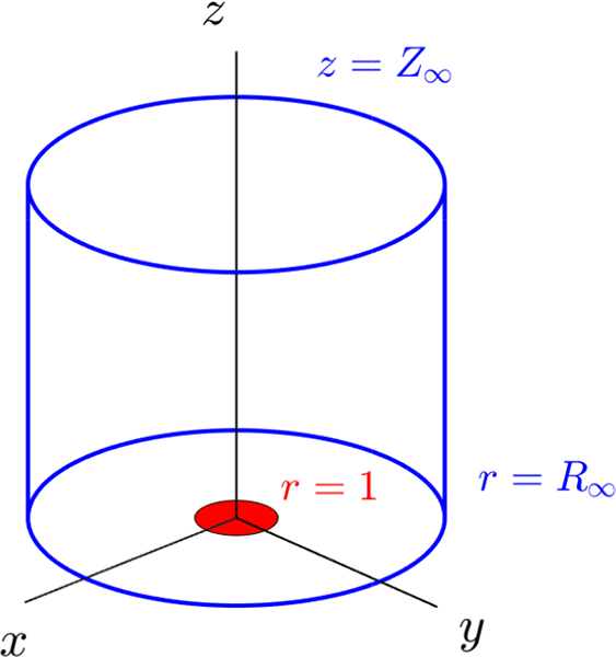


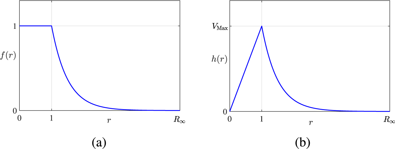


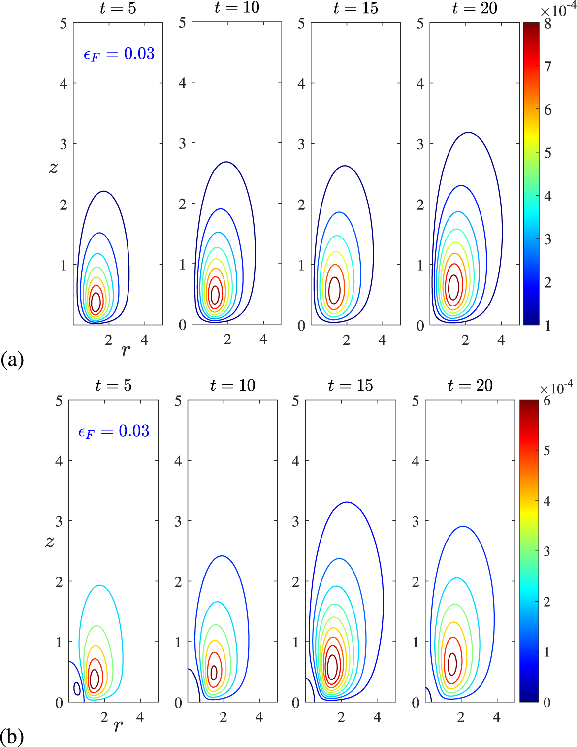


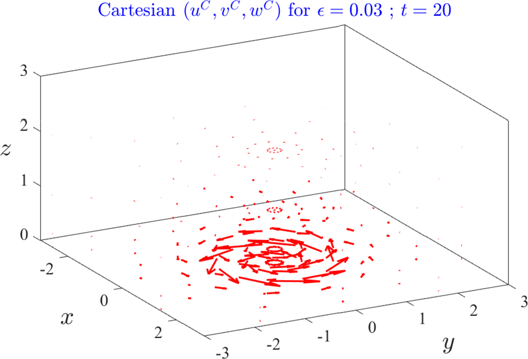


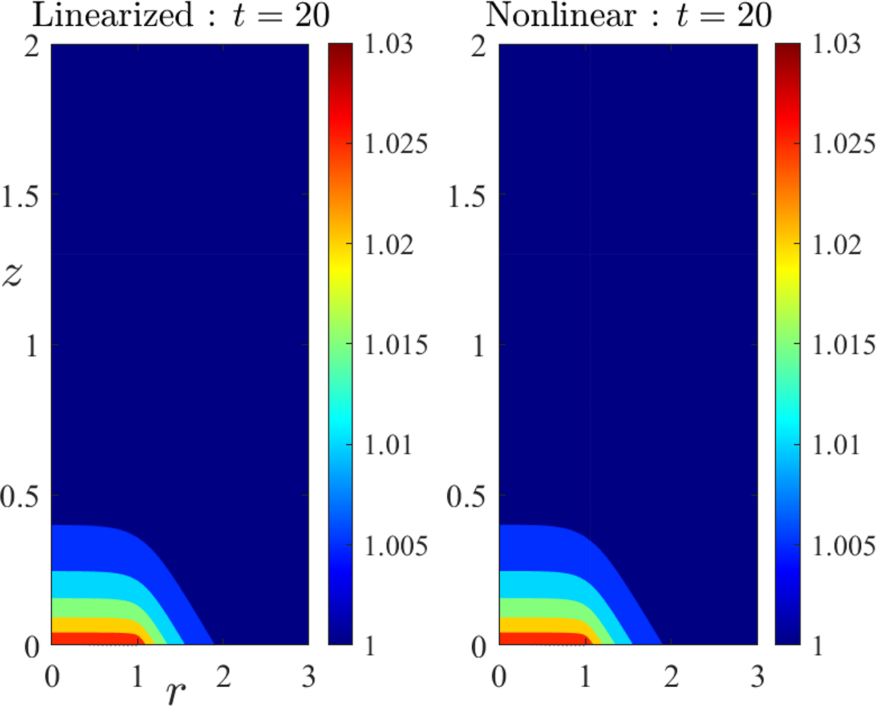


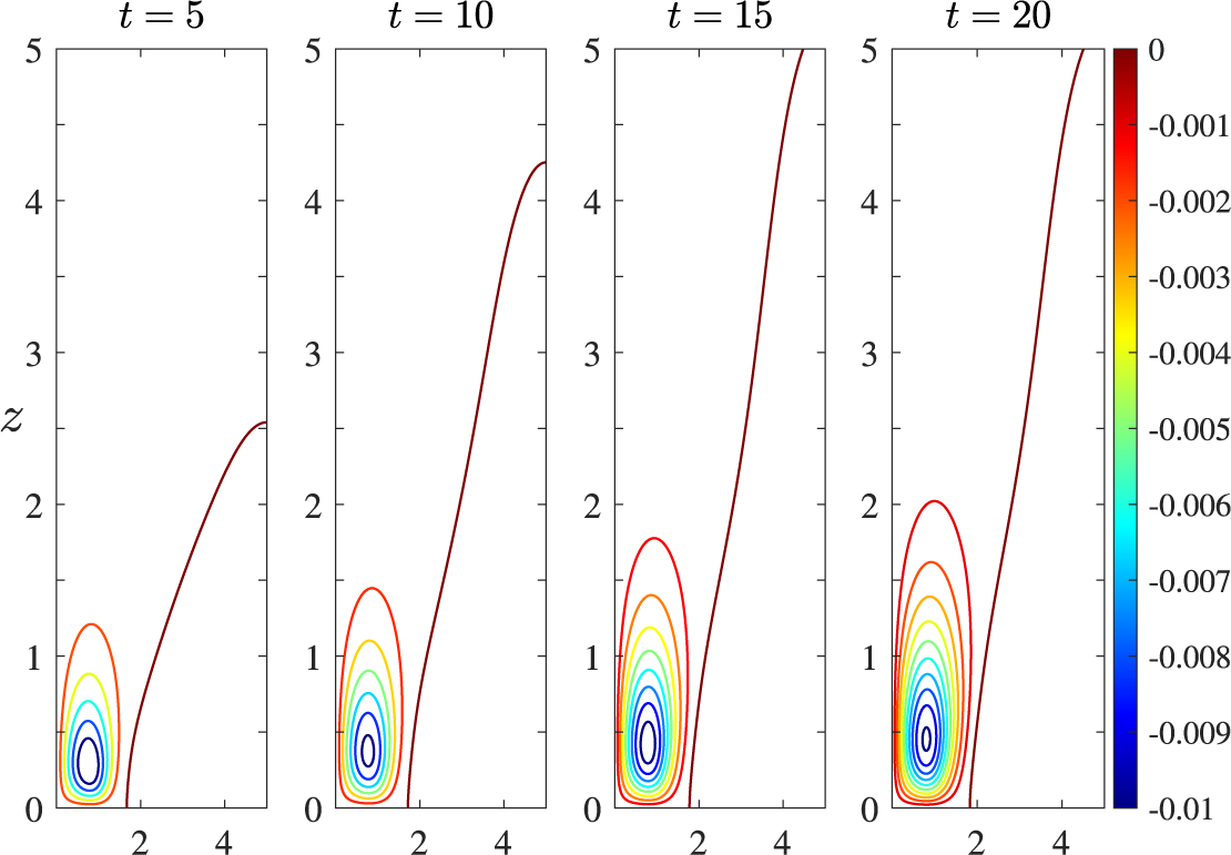


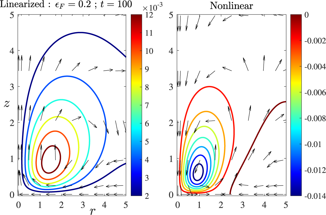


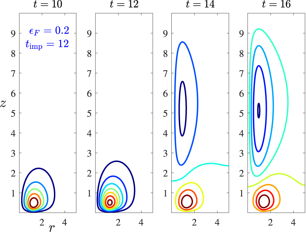


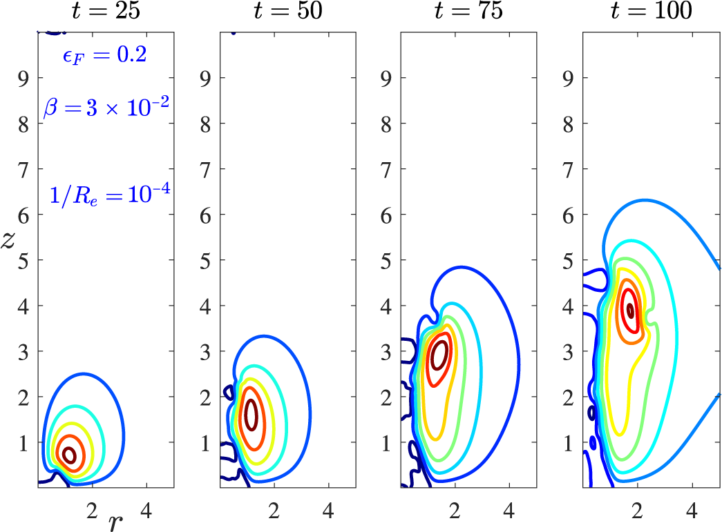


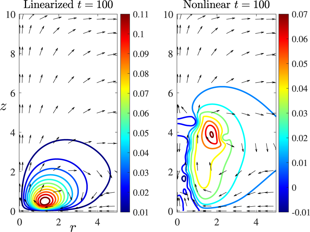


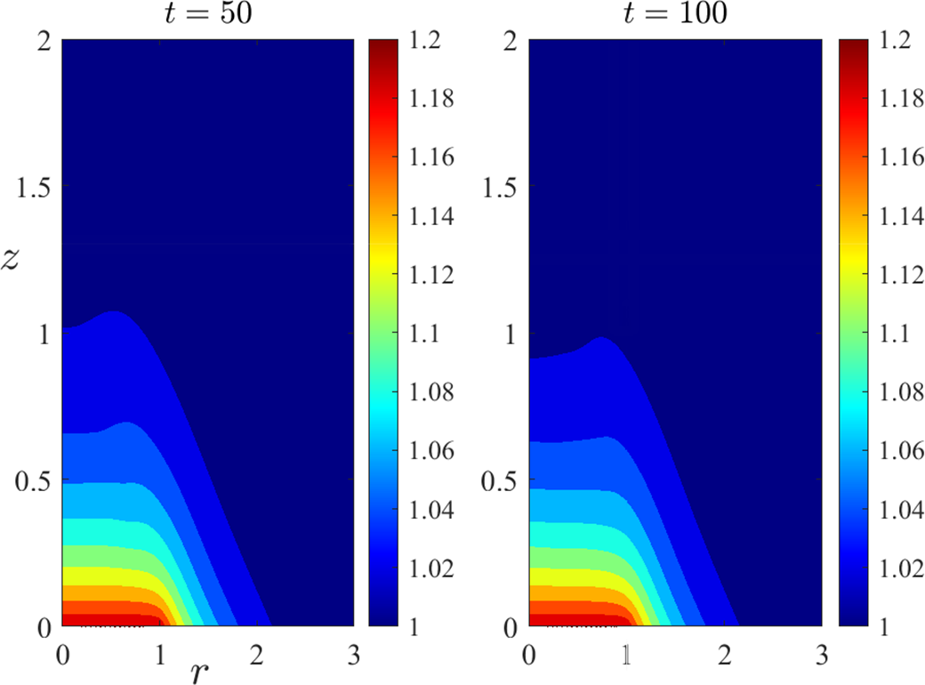


 Open access