

1. Introduction
Cow-calf producers in the southeastern United States are confronted with many complex decisions, one of which is selecting a calving season. Research has shown that a controlled calving season (e.g., in the spring or fall) is more profitable for beef cattle producers than year-round calving (Doye, Popp, and West, Reference Doye, Popp and West2008). However, selecting an optimal calving season depends on a complex set of factors including nutritional demands of brood cows, forage availability, calf weaning weights, calving rates (calves weaned per cow exposed to a bull), seasonality in cattle and feed prices, and labor availability (Bagley et al., Reference Bagley, Carpenter, Feazel, Hembry, Huffman and Koonce1987; Caldwell et al., Reference Caldwell, Coffey, Jennings, Philipp, Young, Tucker and Hubbell2013; Campbell et al., Reference Campbell, Backus, Dixon, Carlisle and Waller2013; Leesburg, Tess, and Griffith, Reference Leesburg, Tess and Griffith2007; Smith et al., Reference Smith, Caldwell, Popp, Coffey, Jennings, Savin and Rosenkrans2012). Most cow-calf producers using a defined calving season in the southeastern United States follow a spring-calving season, beginning in January and ending around mid-March (Campbell et al., Reference Campbell, Backus, Dixon, Carlisle and Waller2013). Cows are typically bred in late spring–early summer (May and June), and calves are weaned in the fall (September and October). An alternative calving season used by southeastern beef cattle producers is birthing calves in fall between mid-September and mid-November (Campbell et al., Reference Campbell, Backus, Dixon, Carlisle and Waller2013). Fall-calving cows are bred in the winter (December and January), and calves are weaned in the spring (April and May).
Nutritional demands are different for spring- and fall-calving cows. The timing of nutritional needs for spring-calving cows more closely matches the growth cycle of warm-season grasses (Bagley et al., Reference Bagley, Carpenter, Feazel, Hembry, Huffman and Koonce1987), which typically break dormancy in early April and grow primarily from mid-May through August (Keyser et al., Reference Keyser, Harper, Bates, Waller and Doxon2011). Warm-season grass growth and development peaks at the time when spring-calving cows require their highest nutritional intake to produce milk for growing calves, maintain body condition, and rebreed. On the other hand, the growth and development of cool-season grasses such as tall fescue more closely matches the nutritional needs of fall-calving cows (Bagley et al., Reference Bagley, Carpenter, Feazel, Hembry, Huffman and Koonce1987). Cool-season grasses grow primarily from late February and early March to May with additional growth from the end of September to November (Keyser et al., Reference Keyser, Harper, Bates, Waller and Doxon2011). Therefore, the nutritional intake requirement for fall-calving cows is highest when the cool-season grass production is peaking.
In Tennessee and much of the southeastern United States, tall fescue is the primary forage used by cattle producers because of suitable growing conditions (Keyser et al., Reference Keyser, Harper, Bates, Waller and Doxon2011). Tall fescue, however, can cause several managerial challenges for beef cattle producers during the summer. Tall fescue can become semidormant in response to summer heat and drought, thereby reducing forage production. Physiological characteristics of tall fescue commonly present during the summer may also negatively affect beef cattle performance (Volenec and Nelson, Reference Volenec, Nelson, Barnes, Nelson, Moore and Collins2007). Cattle grazing on endophyte-infected tall fescue during the summer are likely affected by fescue toxicosis (Volenec and Nelson, Reference Volenec, Nelson, Barnes, Nelson, Moore and Collins2007), which can negatively affect pregnancy rates, weight gains, and net returns of spring-calving cows (Smith et al., Reference Smith, Caldwell, Popp, Coffey, Jennings, Savin and Rosenkrans2012). Thus, fall-calving cows might be more productive in the southeastern United States, even though most cow-calf operators calve in the spring (Campbell et al., Reference Campbell, Backus, Dixon, Carlisle and Waller2013).
Several studies have been conducted in the southern United States to evaluate the effects of calving season on animal performance measures such as 205-day calf weaning weight, calving rate, and cow culling rate (Table 1). Overall, the results of these studies are mixed. The animal performance of spring- and fall-calving herds grazing tall fescue was examined in Arkansas (Caldwell et al., Reference Caldwell, Coffey, Jennings, Philipp, Young, Tucker and Hubbell2013; Smith et al., Reference Smith, Caldwell, Popp, Coffey, Jennings, Savin and Rosenkrans2012) and in Tennessee (Campbell et al., Reference Campbell, Backus, Dixon, Carlisle and Waller2013). The Arkansas studies found that fall-born calves had higher weaning weights than spring-born calves. Conversely, a study in Tennessee found that spring-born calves had higher weaning weights than fall-born calves. In both locations, the calving rate was lower for the spring-calving season, which could be explained by fescue toxicity.
Summary of Studies Evaluating the Animal Performance and Profitability Variables for a Spring- and Fall-Calving Season

a The calving season indicates whether fall or spring calving was higher or lower relative to the comparison calving system.
Note: NA, not applicable; ND, no significant difference.
Several of the aforementioned studies have used animal performance data to evaluate the profitability of the calving season decision. In Louisiana, Bagley et al. (Reference Bagley, Carpenter, Feazel, Hembry, Huffman and Koonce1987) found that fall-born calves produced higher mean net returns than spring born calves. Smith et al. (Reference Smith, Caldwell, Popp, Coffey, Jennings, Savin and Rosenkrans2012) also determined that fall calving produced higher mean partial net returns in Arkansas. Thus, the two studies concluded that fall calving was the most profitable. Campbell et al. (Reference Campbell, Backus, Dixon, Carlisle and Waller2013) found that fall calving produced higher average revenue over the 19-year period in Tennessee than spring calving. This was attributable to the fall-calving herd producing more calves per cow, selling calves at higher prices at weaning, and having to replace fewer cows. Although these studies are insightful, a limitation of these studies was that they did not consider the seasonality of feed and other costs that affect profitability.
The seasonality of beef cattle and feed prices is important when selecting a calving season to maximize profits. Typically, the prices of steer and heifer calves are higher in the spring than in the fall (Julien and Tess, Reference Julien and Tess2002). Fall-born calves weaned in the spring (April and May) may bring higher prices than identical-weight spring-born calves weaned in the fall (September and October). On the other hand, feed costs may be higher for fall-calving cows than for spring-calving cows (Campbell et al., Reference Campbell, Backus, Dixon, Carlisle and Waller2013). Fall-calving cows may require a greater nutritional intake than spring-calving cows because they are bred and nursing a calf in winter.
Research in the southeastern United States that evaluated the profitability of the calving season decision did not assess the potential trade-offs in risk and return of using a fall-calving season rather than a spring-calving season, the predominant defined calving system in Tennessee. Studies evaluating the risk and return to the calving season decision have been conducted for the western and northwestern United States (Evans et al., Reference Evans, Sperow, D'Souza and Rayburn2007; Leesburg, Tess, and Griffith, Reference Leesburg, Tess and Griffith2007; Strauch, Peck, and Held, Reference Strauch, Peck and Held2010) and Canada (Khakbazan et al., Reference Khakbazan, Carew, Scott, Chiang, Block, Robins, Durunna and Huang2014; Sirski, Reference Sirski2012), but not the southeastern United States. Information is needed about how calf weights at marketing, beef prices, feed costs, and other factors associated with spring and fall calving influence the profitability and risk (i.e., variability of profits) of cow-calf production in the southeastern United States. If such information were available, cow-calf producers in Tennessee and other southeastern states would have better economic information to make decisions about the appropriate calving season.
Therefore, the objective of this research was to determine the profitability and risk for spring- and fall-calving seasons for beef cattle in Tennessee while considering the seasonality of cattle and feed prices for least-cost feed rations. To accomplish this, simulation models were developed considering production and price risks to find a distribution of net returns for spring- and fall-calving seasons. Data for the spring- and fall-calving cows came from a 19-year study located in Tennessee.
2. Conceptual Framework
Beef cattle producers are subject to several sources of risk, but production and price risks are likely the two primary sources on an annual basis (Kay, Edwards, and Duffy, Reference Kay, Edwards and Duffy2012). Production risk is defined as the uncertainty around annual animal production such as death loss, pregnancy rates, and weaning weights (Kay, Edwards, and Duffy, Reference Kay, Edwards and Duffy2012). Because approximately 70% of spring-born calves are typically marketed immediately after weaning in the southeastern United States (Lacy, Knight, and Mckissick, Reference Lacy, Knight and Mckissick2012), the primary source of production risk for fall- versus spring-born calves is from the differences in the mean and variance of calf weaning weights (Caldwell et al., Reference Caldwell, Coffey, Jennings, Philipp, Young, Tucker and Hubbell2013; Campbell et al., Reference Campbell, Backus, Dixon, Carlisle and Waller2013; Smith et al., Reference Smith, Caldwell, Popp, Coffey, Jennings, Savin and Rosenkrans2012). Nutritional demands for spring- and fall-calving cows and the seasonal supply of forage also vary with the calving season, thereby affecting supplemental feed costs for brood cows during the winter when pasture is dormant (Bagley et al., Reference Bagley, Carpenter, Feazel, Hembry, Huffman and Koonce1987; Campbell et al., Reference Campbell, Backus, Dixon, Carlisle and Waller2013; Keyser et al., Reference Keyser, Harper, Bates, Waller and Doxon2011). Price risk is associated with changes in beef cattle and feed prices from year to year and from month to month and is also an important factor influencing the risk and return to the calving season decision (Campbell et al., Reference Campbell, Backus, Dixon, Carlisle and Waller2013; Julien and Tess, Reference Julien and Tess2002).
When incorporating risk in a cow-calf operator's decision-making framework, the optimal calving season is a function of expected net returns and the variability of net returns. Therefore, a producer's decision-making framework is to select a calving season that maximizes the utility, defined as Ui (π i , r), where πi is the expected annual net returns for the ith calving season (fall calving or spring calving) and r is the producer's risk preference level (Hardaker et al., Reference Hardaker, Richardson, Lien and Schumann2004). A cow-calf producer will choose spring calving if the expected utility is higher than the expected utility of the fall calving: E[U S (π S , r)] > E[U F (π F , r)], where S is the spring-calving season and F is the fall-calving season. Conversely, a cow-calf producer will follow a fall-calving season if the expected utility is higher than the expected utility of spring calving: E[U S (π S , r)] < E[U F (π F , r)].
3. Methods
3.1. Simulation Model
Expected revenue for a cow-calf producer is earned from selling steers, heifers, and culled cows with the prices of these animals changing each month. The size of the calves at weaning, calf death losses, and the number of brood cows culled are also important variables affecting revenue and may vary by calving season. Commonly incurred costs in cow-calf production include land, labor, pasture, feed, and animal health inputs, as well as the fees incurred from trucking and marketing livestock. When selecting between spring and fall calving, an important cost that a producer should consider is supplemental feed costs when pasture is dormant in winter (Campbell et al., Reference Campbell, Backus, Dixon, Carlisle and Waller2013). Although other costs are often similar across calving seasons, the quantity of feed varies by calving season due to different nutritional requirements for cows in each calving season.
Given the aforementioned factors influencing the profitability and riskiness of cow-calf production, a simulation model was developed to estimate stochastic net returns above production costs considering seasonality of feed and beef prices for spring- and fall-calving seasons, which is expressed as:
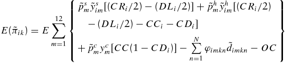 $$\begin{equation}
E({\tilde \pi _{ik}}) = E\sum\limits_{m = 1}^{12} {\left\{ \begin{array}{l} \tilde p_m^s\tilde y_{im}^s[(C{R_i}/2)- (D{L_i}/2)] + \tilde p_m^h\tilde y_{im}^h[(C{R_i}/2)\\[5pt]
\quad -\, (D{L_i}/2) - C{C_i} - C{D_i}]\\[5pt]
+\, \tilde p_m^cy_m^c[CC(1 - CD{}_i)] - \sum\limits_{n = 1}^N {{\varphi _{imkn}}{{\tilde d}_{imkn}}} - OC \end{array} \right\}}
\end{equation}$$
$$\begin{equation}
E({\tilde \pi _{ik}}) = E\sum\limits_{m = 1}^{12} {\left\{ \begin{array}{l} \tilde p_m^s\tilde y_{im}^s[(C{R_i}/2)- (D{L_i}/2)] + \tilde p_m^h\tilde y_{im}^h[(C{R_i}/2)\\[5pt]
\quad -\, (D{L_i}/2) - C{C_i} - C{D_i}]\\[5pt]
+\, \tilde p_m^cy_m^c[CC(1 - CD{}_i)] - \sum\limits_{n = 1}^N {{\varphi _{imkn}}{{\tilde d}_{imkn}}} - OC \end{array} \right\}}
\end{equation}$$
where ${\tilde \pi _{ik}}$
is the uncertain net returns above production costs ($/head) for the ith calving season (fall calving or spring calving) for the kth (k = 1,. . ., K) ration;
${\tilde \pi _{ik}}$
is the uncertain net returns above production costs ($/head) for the ith calving season (fall calving or spring calving) for the kth (k = 1,. . ., K) ration; $\tilde p_m^s$
is the uncertain price of 500–600 lb. steer calves ($/lb.);
$\tilde p_m^s$
is the uncertain price of 500–600 lb. steer calves ($/lb.); $\tilde y_{im}^s$
is the uncertain weight of steer calves (lb./head); CRi
is the calving rate (0 ≤ CRi
≤ 1); DLi
is the death loss for calves (0 ≤ DLi
≤ 1);
$\tilde y_{im}^s$
is the uncertain weight of steer calves (lb./head); CRi
is the calving rate (0 ≤ CRi
≤ 1); DLi
is the death loss for calves (0 ≤ DLi
≤ 1); $\tilde p_m^h$
is the uncertain price of 400–500 lb. heifer calves ($/lb.);
$\tilde p_m^h$
is the uncertain price of 400–500 lb. heifer calves ($/lb.); $\tilde y_{im}^h$
is the uncertain weight of heifer calves (lb./head); CCi
is the proportion (0 ≤ CC ≤ 1) of cows culled, which is also the proportion of heifer replacement retained per cow; CDi
is the cow death loss (0 ≤ CDi
≤ 1);
$\tilde y_{im}^h$
is the uncertain weight of heifer calves (lb./head); CCi
is the proportion (0 ≤ CC ≤ 1) of cows culled, which is also the proportion of heifer replacement retained per cow; CDi
is the cow death loss (0 ≤ CDi
≤ 1); $\tilde p_m^c$
is the uncertain price of 1,100–1,600 lb. culled cows ($/lb.);
$\tilde p_m^c$
is the uncertain price of 1,100–1,600 lb. culled cows ($/lb.); ${\tilde d_{imkn}}$
is the uncertain price of the nth ingredient ($/lb.); ϕimkn
is the quantity (lb./head) of the nth (n = 1,. . ., N) ingredient; and OC are all other annual production costs ($/head), which are likely similar across calving seasons and likely include marketing, trucking, animal health, land, salt, and minerals. Calving rate and death loss for calves were divided by 2 because half the calves were assumed to be steers and half were assumed to be heifers (Department of Agricultural and Resource Economics, University of Tennessee, 2016).
${\tilde d_{imkn}}$
is the uncertain price of the nth ingredient ($/lb.); ϕimkn
is the quantity (lb./head) of the nth (n = 1,. . ., N) ingredient; and OC are all other annual production costs ($/head), which are likely similar across calving seasons and likely include marketing, trucking, animal health, land, salt, and minerals. Calving rate and death loss for calves were divided by 2 because half the calves were assumed to be steers and half were assumed to be heifers (Department of Agricultural and Resource Economics, University of Tennessee, 2016).
Net returns above production costs were simulated for eight calving season, weaning month, and supplemental feed ration scenarios. Spring-born calves were assumed to be weaned and sold in either September or October. Fall-born calves were presumed to be weaned and sold in either April or May. Because data on supplemental feed requirements for brood cows were not available from the study for the simulation, two least-cost feed rations were developed for each calving season and weaning month scenario to provide estimates of supplemental feed quantities for ϕimkn in equation (1). The average and standard deviation of weaning weights for steers and heifers were calculated from animal data first reported by Campbell et al. (Reference Campbell, Backus, Dixon, Carlisle and Waller2013) and used to create a normal distribution from which to draw calf weights for the simulation. Prices for steers, heifers, culled cows, and ration ingredients were randomly drawn from a multivariate empirical distribution derived using historical price data and following Richardson, Klose, and Gray's (Reference Richardson, Klose and Gray2000) estimation procedure for a multivariate empirical distribution. Simulation and Econometrics to Analyze Risk (SIMETAR) was used to develop the distributions and perform the simulations (Richardson, Schumann, and Feldman, Reference Richardson, Schumann and Feldman2008). A total of 5,000 net return observations were simulated for each of the eight scenarios (2 calving seasons × 2 weaning months × 2 feed rations).
3.2. Least-Cost Ration
Two supplemental feed rations for each calving season and weaning month scenario were developed to meet the nutrient requirements for cows in the spring- and fall-calving herds for December, January, February, and March. Rations were only developed for winter and assumed that both spring- and fall-calving herds had adequate nutrition available through grazing tall fescue pastures the remaining months of the year. Nutritional requirements differ by month and by calving season because of different gestation cycles (George, Nader, and Dunbar, Reference George, Nader and Dunbar2001), affecting the quantity of feed needed by month.
Rations were put together to meet the predetermined nutritional needs for cows in each calving herd using the National Research Council's (NRC) Nutrient Requirements of Beef Cattle (NRC, 1996). The NRC program determined the minimal nutritional needs for a cow based on animal description, environmental factors, pasture management, and feed diet evaluation. The animal description variables were age, body weight, body condition score, calf birth weight, peak milk production, milk fat, milk protein, days pregnant, and days in milk. The environmental factors contained night cooling, hair depth, and monthly average temperature. Pasture management variables included additives, pasture unit size, pasture mass, and days on pasture. In the diet evaluation section, the NRC program focuses on balancing a cow's monthly required dry matter intake (DMI), energy (NEm), and metabolizable protein (MP) using the available feed ration ingredients specified in the program. The size of the cow, time in gestation, and milk production influence the minimal nutrient intake needed per cow per day. Energy and protein requirements increased approximately 60 days into lactation, known also as the peak lactation period after calving (George, Nader, and Dunbar, Reference George, Nader and Dunbar2001). There was also a rise in energy and protein requirements during the last 60 days of gestation (George, Nader, and Dunbar, Reference George, Nader and Dunbar2001). The specific parameters for animal description, environmental factors, pasture management, and feed diet evaluation used in this study have been described by Henry (Reference Henry2015).
Ingredients for feed rations can be selected by producers based on several criteria. The accessibility and price of the ingredients are likely two of the most important criteria for selecting feed rations. Therefore, the least-cost rations (K = 2) were constructed by selecting from eight commonly accessible ingredients in Tennessee, including corn gluten feed, corn silage, dried distillers grains, soybean hulls, whole cottonseed, rice bran, and wheat middlings. The two least-cost rations were constructed to select across the eight ingredients: (1) when at least 20 lb./day of orchard grass hay was fed and (2) when orchard grass hay was not required to be fed. A linear programming model was constructed to select across eight feed ingredients to build the two least-cost feed rations. The objective was to find the combination and quantity (ϕimk ) of the eight ingredients that minimized costs while providing a cow the minimum amount of DMI, MP, and NEm per month, which is expressed as follows:
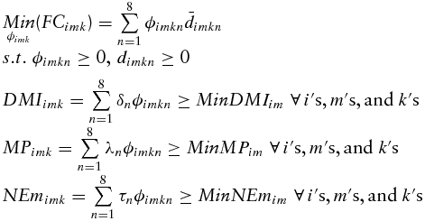 $$\begin{equation}
\begin{array}{l} \mathop {{{\it Min}}}\limits_{{\phi _{imk}}} ({\it FC}{_{imk}}) = \sum\limits_{n = 1}^8 {{\phi _{imkn}}{{\bar d}_{imkn}}} \\[4pt]
s.t.\ {\phi _{imkn}} \ge 0,\,{d_{imkn}} \ge 0\\[4pt] {\it DMI}{_{imk}} = \sum\limits_{n = 1}^8 {{\delta _n}{\phi _{imkn}}} \ge {\it MinDM}{I_{im}}\,\,\forall \,i'{\rm{s,}}\,m'{\rm{s, and }}\;k{\rm{'s}}\\[4pt] {\it MP}{_{imk}} = \sum\limits_{n = 1}^8 {{\lambda _n}{\phi _{imkn}}} \ge {\it MinM}{P_{im}}\,\,\forall \,i'{\rm{s,}}\,m'{\rm{s, and }}\;k{\rm{'s}}\\[4pt] {\it NE}{m_{imk}} = \sum\limits_{n = 1}^8 {{\tau _n}{\phi _{imkn}}} \ge {\it MinNE}{m_{im}}\,\,\forall \,i'{\rm{s,}}\,m'{\rm{s, and }}\;k{\rm{'s}} \end{array}
\end{equation}$$
$$\begin{equation}
\begin{array}{l} \mathop {{{\it Min}}}\limits_{{\phi _{imk}}} ({\it FC}{_{imk}}) = \sum\limits_{n = 1}^8 {{\phi _{imkn}}{{\bar d}_{imkn}}} \\[4pt]
s.t.\ {\phi _{imkn}} \ge 0,\,{d_{imkn}} \ge 0\\[4pt] {\it DMI}{_{imk}} = \sum\limits_{n = 1}^8 {{\delta _n}{\phi _{imkn}}} \ge {\it MinDM}{I_{im}}\,\,\forall \,i'{\rm{s,}}\,m'{\rm{s, and }}\;k{\rm{'s}}\\[4pt] {\it MP}{_{imk}} = \sum\limits_{n = 1}^8 {{\lambda _n}{\phi _{imkn}}} \ge {\it MinM}{P_{im}}\,\,\forall \,i'{\rm{s,}}\,m'{\rm{s, and }}\;k{\rm{'s}}\\[4pt] {\it NE}{m_{imk}} = \sum\limits_{n = 1}^8 {{\tau _n}{\phi _{imkn}}} \ge {\it MinNE}{m_{im}}\,\,\forall \,i'{\rm{s,}}\,m'{\rm{s, and }}\;k{\rm{'s}} \end{array}
\end{equation}$$
where FCimk
is the feed cost ($/head) in the mth month of the kth ration for the ith herd; ${\bar d_{imkn}}$
is average price of the nth ingredient ($/lb.); DMIimk
is the DMI (lb./day) in the mth month of the kth ration for the ith herd; δn
is the percentage of ingredient n that is dry matter; MinDMIim
is the minimum level of DMI (lb./day) needed by a cow; MPimk
is the MP (g/day); λn
is the percentage of ingredient n that is MP; MinMPim
is the minimal MP (g/day) needed by a cow; NEmimk
is the NEm (Mcal/day); τn
is the percentage of ingredient n that is NEm; and MinNEmim
is the minimal NEm (Mcal/day) needed by a cow. The coefficients for the quantity of the ingredient in 1 lb. of the ration that minimizes the cost of the ration were substituted into the simulation model.
${\bar d_{imkn}}$
is average price of the nth ingredient ($/lb.); DMIimk
is the DMI (lb./day) in the mth month of the kth ration for the ith herd; δn
is the percentage of ingredient n that is dry matter; MinDMIim
is the minimum level of DMI (lb./day) needed by a cow; MPimk
is the MP (g/day); λn
is the percentage of ingredient n that is MP; MinMPim
is the minimal MP (g/day) needed by a cow; NEmimk
is the NEm (Mcal/day); τn
is the percentage of ingredient n that is NEm; and MinNEmim
is the minimal NEm (Mcal/day) needed by a cow. The coefficients for the quantity of the ingredient in 1 lb. of the ration that minimizes the cost of the ration were substituted into the simulation model.
3.3. Risk Analysis
A common approach to comparing net returns and variability of net returns for different agricultural production management scenarios is to use stochastic dominance, which compares the cumulative distribution function (CDF) of net returns for all scenarios (Chavas, Reference Chavas2004). In first-degree stochastic dominance, the scenario with CDF F dominates another scenario with CDF G if F(π) ⩽ G(π)∀π. First-degree stochastic dominance often does not find one scenario to clearly be preferred over another; therefore, second-degree stochastic dominance adds the restriction that producers are risk averse, which increases the chance of finding a preferable scenario (Chavas, Reference Chavas2004). Second-degree stochastic dominance states that the scenario with CDF F dominates another scenario with CDF G if ∫F(π)dπ ⩽ ∫G(π)dπ∀π.
If there is not a clear dominant calving season, weaning month, and feed ration strategy using first- and second-degree stochastic dominance, then stochastic efficiency with respect to a function (SERF) was used to rank the management scenarios over a range of absolute risk aversion (Hardaker et al., Reference Hardaker, Richardson, Lien and Schumann2004). SERF analysis is a common method used to compare the risk of different production decisions (Barham et al., Reference Barham, Robinson, Richardson and Rister2011; Williams et al., Reference Williams, Saffert, Barnaby, Llewelyn and Langemeier2014). It requires the specification of a utility function, $U\;({\tilde \pi _{ik}},r)$
, which is a function of the distribution of net returns and absolute risk-preference level r. The utility function was used to find the certainty equivalent (CE), which is defined as the guaranteed return a person is willing to take rather than taking a gamble for a higher, but uncertain, return. A rational decision maker who is risk averse has a CE that is less than the expected value of the uncertain return. That is, a cow-calf producer who is risk averse would be willing to take a lower return with certainty instead of a higher return with uncertainty. The calving season and feed ration with the highest CE at a given level of risk aversion is the optimal calving season and maximizes utility.
$U\;({\tilde \pi _{ik}},r)$
, which is a function of the distribution of net returns and absolute risk-preference level r. The utility function was used to find the certainty equivalent (CE), which is defined as the guaranteed return a person is willing to take rather than taking a gamble for a higher, but uncertain, return. A rational decision maker who is risk averse has a CE that is less than the expected value of the uncertain return. That is, a cow-calf producer who is risk averse would be willing to take a lower return with certainty instead of a higher return with uncertainty. The calving season and feed ration with the highest CE at a given level of risk aversion is the optimal calving season and maximizes utility.
A negative exponential utility function was used in this analysis, which specifies a constant absolute risk-aversion coefficient (ARAC) to calculate the CE (Pratt, Reference Pratt1964). The ARAC represents the ratio of derivatives of the person's utility function ra (r) = −U''(r)/U'(r). Following Hardaker et al. (Reference Hardaker, Richardson, Lien and Schumann2004), a vector of CEs was derived bounded by a low and a high ARAC. The lower bound ARAC was 0, meaning the producer was risk neutral and the calving seasons and feed ration scenario with the highest expected net returns was preferred. The upper bound ARAC was found by dividing 4 by the average net returns for all the calving seasons and feed ration scenarios, which was proposed by Hardaker et al. (Reference Hardaker, Richardson, Lien and Schumann2004) to find the extremely risk-averse decision maker.
ARAC values ranged from 0.0 for risk neutral to 0.03 for highly risk averse in the analysis. Taking the difference between CEs of any two alternatives was defined as the utility-weighted risk premium. The risk premium is the minimum amount of money a decision maker would have to be paid to switch from the calving season and feed ration scenario with the greatest CE to the alternative calving season and feed ration scenario with the lesser CE. The SERF analysis was also conducted in SIMETAR (Richardson, Schumann, Feldman, Reference Richardson, Schumann and Feldman2008).
4. Data
4.1. Animal Production
The data for the spring- and fall-calving cows originates from Ames Plantation Research and Education Center, near Grand Junction, Tennessee, from 1990 to 2008. The spring- and fall-calving cows consisted of both commercial and purebred Angus cattle. The commercial cattle were predominantly Angus with Simmental and Hereford influence. Bulls and replacement heifers for the purebred Angus herd were developed at Ames Plantation; however, bulls were purchased to maintain the genetic diversity of the herd. The bulls for the commercial cattle were of purebred Angus origin. Cows were not switched between the spring- and fall-calving herds. The spring-calving herd calved from mid-February through mid-April. The fall-calving herd calved from mid-September through mid-November.
Both herds primarily grazed endophyte-infected tall fescue and were supplemented with free choice mineral and corn silage year-round as needed. The quantity of corn silage and choice mineral fed to cattle in each herd was not recorded, which is a limitation of this analysis and is why we had to generate feed costs using the least-cost feed ration model. Cows were primarily culled because of failure to rebreed; however, poor calf performance and old age also factored into the decision to cull a cow. Poor calf performance was based on total weight gain compared with the other calves of the same age. Over the 19-year period, the spring herd totaled 478 individual cows with 1,534 individual calves born, and the fall herd totaled 474 individual cows with 1,727 calves born. These cow and calf totals reflect the number of cows and calves that were included in the herd at some point over the 19-year period of the data.
The cow data included identification number, breed, calving herd, sire, dam, and date of birth. Unfortunately, records were not kept for cows that did not calve; thus, percent calf rate could not be directly calculated. Data for the calves included calf number, date of birth, sex, sire, number of calves the cow has calved, average daily gain, birth weight, and weaning weight. Weaning weight is a common measure for calf growth potential and the mothering ability of the dam. Actual weaning weights, however, are influenced by the age of the calf at weaning, sex of the calf, and age of the dam. Therefore, a common practice is to calculate the 205-day adjusted weaning weights, which gives an adjusted weaning weight for calves of different ages. The adjusted 205-day weaning weight used in this study was calculated following the guidelines of the Beef Improvement Federation (2010). Table 2 includes the average birth weight and adjusted 205-day weaning weight by steer and heifer calves in the spring- and fall-calving herds.
Average Birth Weight (in lb.) and Adjusted 205-Day Weaning Weight (in lb.) by Calving Season and Calf Sex at Grand Junction, Tennessee, from 1990 to 2008
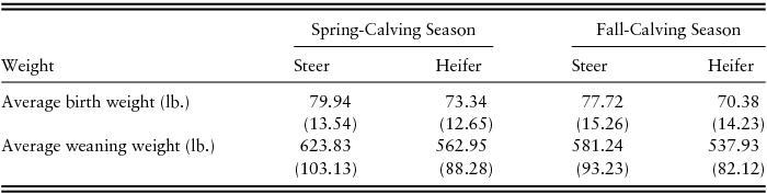
Note: Standard deviations are noted in parentheses.
4.2. Budgets and Prices
Budgets were constructed to calculate production costs on a per head basis for the stochastic simulation of net returns in equation (1) and followed procedures and assumptions in University of Tennessee Extension livestock budgets (Department of Agricultural and Resource Economics, University of Tennessee, 2016). Calf death loss, cow death loss, calving rate, cull percentage, and culled cow weights were assumed from the literature and enterprise budgets because these data were not available from the animal performance data used in this study. The culled cow percentage of 16%, cow death loss of 1%, calving rate of 90%, and culled cow weight of 1,100 lb. were assumed for both the spring- and fall-calving seasons (Department of Agricultural and Resource Economics, University of Tennessee, 2016). Death loss for calves was assumed to be 5% for the spring-born calves and 3% for the fall-born calves, which was within the range found in the literature (Bagley et al., Reference Bagley, Carpenter, Feazel, Hembry, Huffman and Koonce1987). Not having death loss, calving rate, and culled cow percentage in the data is a limitation of this analysis; therefore, these assumptions were made using the best available data.
Monthly Tennessee beef price data for the steers, heifers, and culled cows for the simulation were collected from 1990 to 2013 (U.S. Department of Agriculture, Agricultural Marketing Service [USDA-AMS], 2012). Monthly prices for the ingredients of the feed rations reported at Memphis, Tennessee, and St. Louis, Missouri (the nearby reporting locations to Tennessee), were also collected from USDA-AMS (2012); however, the prices were only available from 2000 to 2013 for December, January, February, and March. All beef and feed ingredient prices were adjusted into 2013 dollar values using the Consumer Price Index (U.S. Department of Labor, Bureau of Labor Statistics, 2013). Table 3 presents the real monthly average and standard deviation for price of steers, heifers, and culled cows. Table 4 presents the real monthly average and standard deviation for prices of orchard grass hay, corn gluten feed, corn silage, dried distillers grains, soybean hulls, whole cottonseed, rice bran, and wheat middlings in the months of December, January, February, and March (USDA-AMS, 2012). In the simulation, prices for steers, heifers, culled cows, and ration ingredients were randomly drawn from a multivariate empirical distribution.
Average Monthly Real Price (in $/cwt.) for Steers (500–600 lb.), Heifers (500–600 lb.), and Culled Cows (1,100–1,600 lb.) in Tennessee from 1989 to 2013 in 2013 Dollars

Average Monthly Real Prices ($/dry ton) for Feed Ration Ingredients from 2000 to 2013 in 2013 Dollars

5. Results
5.1. Least-Cost Rations
Table 5 shows the quantity (lb./day) of each ingredient in the two least-cost feed rations that provided the minimum requirements of DMI, MP, and NEm by month and calving season. Both of the rations modeled selected the ingredients of orchard grass, corn gluten, corn silage, rice bran, and wheat middlings. Spring-calving cows required less daily feed in December and January than fall-calving cows. The spring-calving cows were transitioning from a late-gestation and no lactation period into a calving and lactation period in December and January, and the fall-calving cows were moving from a breeding and lactation period to an early gestation and lactation period, which required higher levels of MP and NEm. However, in February and March, spring-calving cows required higher feed intake because the spring-calving cows were reaching the peak lactation period. Overall, fall-calving cows required more feed from December through March than spring-calving cows, which has a higher total cost for feed. For both calving seasons, relaxing the constraint of a minimum of 20 lb./day of orchard grass hay being fed reduced the total feed required and lowered the total cost of feed, resulting in a shift to feeding more corn silage and less orchard grass hay. We substituted the quantities for each ration into the budgets for the two calving seasons with two weaning months.
Amount of Ingredients Fed (dry lb./day) and Total Cost in each of the Least-Cost Winter Feed Rations by Calving Season and Month

Source: National Research Council (1996).
5.2. Simulated Net Returns
The average and standard deviation of simulated net returns (in $/head) under the least-cost rations by calving season and weaning month are presented in Table 6. For the spring-calving season, expected net returns were higher when there was not a minimum quantity of orchard grass hay fed for both weaning months, but weaning in September (Spring_Sept_NHC) was more profitable than weaning in October (Spring_Oct_NHC). A spring-calving cow that was fed a ration without the orchard grass hay constraint and weaned in September had the highest expected net returns ($10.03/head), but this scenario also had the highest variability in net returns for the spring-calving scenarios.
Summary Statistics of Simulated Net Returns by Calving Season, Least-Cost Winter Feed Ration, and Weaning Month

a Minimum of 20 lb./day of orchard grass hay.
Similarly, feeding a fall-calving cow a ration with no minimum quantity of orchard grass hay had higher expected net returns and higher variability of net returns than feeding a ration with a minimum quantity of orchard grass hay. Weaning fall-born calves in April produced higher expected net returns and higher variability in net returns than weaning in May. A fall-calving cow that was not fed a minimum amount of orchard grass hay and weaned in April (Fall_April_NHC) had the highest expected net returns ($37.92/head) but also had the most variability in net returns. A fall-calving cow that was fed a minimum amount of orchard grass hay and weaned in May (Fall_May_HC) had the lowest variability of net returns but also had the lowest expected net returns for the fall-calving scenarios.
A profit-maximizing beef cattle producer would select fall calving over spring calving regardless of the feed ration and weaning month given the scenarios considered (Table 6). Caldwell et al. (Reference Caldwell, Coffey, Jennings, Philipp, Young, Tucker and Hubbell2013) and Smith et al. (Reference Smith, Caldwell, Popp, Coffey, Jennings, Savin and Rosenkrans2012) also found fall calving had higher net returns than spring calving in Arkansas. The spring-calving cows had heavier calves at weaning (Table 2) and lower feed costs than the fall-calving cows (Table 5); however, cattle prices at weaning were higher for calves born in the fall (Table 3). The higher prices of steer and heifer calves captured by fall-born calves were able to cover the higher feed expenses and lighter weaning weights by the fall-born calves. This suggests that seasonality of feed and beef prices was the primary factor affecting the results.
5.3. Risk Analysis of Net Returns
Figures 1 and 2, respectively, present the CDFs of net returns for each calving season and weaning month for supplemental feed rations with and without the orchard grass hay constraint. Fall calving dominates spring calving by first-degree stochastic dominance because the cumulative probability of fall calving at all outcomes was less than the cumulative probability of spring calving. Therefore, fall calving was a risk efficient management strategy regardless of producer risk preference. Fall calving may provide risk management benefits for cow-calf producers by reducing the probability of negative net returns. For example, the probability of a loss was reduced from approximately a 61% chance for spring calves sold in September to approximately a 34% chance for fall calves sold in April, assuming no minimum hay constraint in the supplemental feed ration (Table 6).
Cumulative Distribution Function of Net Returns of Spring and Fall Calving with Least-Cost Winter Feed Ration with Hay Constraint (note: Spring_Sept_HC = spring-calving cow that was fed the ration with a hay constraint and calf weaned in September; Spring_Oct_HC = spring-calving cow that was fed the ration with a hay constraint and calf weaned in October; Fall_Apr_HC = fall-calving cow that was fed the ration with a hay constraint and calf weaned in April; and Fall_May_HC = fall-calving cow that was fed the ration with a hay constraint and calf weaned in May)

Cumulative Distribution Function of Net Returns of Spring and Fall Calving with Least-Cost Winter Feed Ration without Hay Constraint (note: Spring_Sept_NHC = spring-calving cow that was fed the ration without a hay constraint and calf weaned in September; Spring_Oct_NHC = spring-calving cow that was fed the ration without a hay constraint and calf weaned in October; Fall_Apr_NHC = fall-calving cow that was fed the ration with a hay constraint and calf weaned in April; and Fall_May_NHC = fall-calving cow that was fed the ration without a hay constraint and calf weaned in May)

The value of the reduced chance of a loss with fall calving can be determined for different ARAC levels using the utility-weighted risk premiums presented in Figure 3. The value of a reduced chance of loss for a moderately risk-averse (ARAC = 0.016) producer was approximately $36/head for fall calves sold in April relative to spring calves sold in September assuming no minimum hay constraint in the supplemental feed ration. By comparison, a highly risk-averse (ARAC 0.03) producer would be expected to place a value of $58/head for fall calves sold in April. Higher calf prices in the spring when calves were sold reduced the probability of a net return loss for fall calving in the simulation analysis.
Utility-Weighted Risk Premiums for Spring- and Fall-Calving Herds under Least-Cost Winter Feed Ration (note: Spring_Sept_NHC = spring-calving cow that was fed the ration without a hay constraint and calf weaned in September; Spring_Oct_NHC = spring-calving cow that was fed the ration without a hay constraint and calf weaned in October; Fall_Apr_NHC = fall-calving cow that was fed the ration with a hay constraint and calf weaned in April; and Fall_May_NHC = fall-calving cow that was fed the ration without a hay constraint and calf weaned in May)

The CDFs in Figures 1 and 2 also show that first- and second-degree stochastic dominance does not exist for the weaning month because the CDFs intersect. SERF was used to determine the combination of calving season, feed ration, and weaning month preferred by beef cattle producers at different levels of absolute risk aversion by calculating CEs. Figure 3 shows the risk premiums for each scenario for the least-cost feed rations. The fall-calving season, regardless of the ration and weaning month, was preferred over the spring-calving season for all levels of risk aversion. Within the fall-calving season, a risk-neutral (ARAC = 0) to moderately risk-averse (ARAC = 0.016) producer would prefer to wean in April and feed a ration that does not require a minimum amount of orchard grass hay (Fall_April_NHC). However, a producer who was moderately risk averse (ARAC = 0.016) to highly risk averse (ARAC 0.03) would select a fall-calving season that weans in May and does not feed a minimum amount of orchard grass hay (Fall_May_NHC).
For spring calving, the supplemental rations that required a minimum amount of orchard grass hay had lower expected net returns and lower standard deviations than rations that did not require a minimum amount of orchard grass hay. As risk aversion increases, a producer would prefer a ration that required a minimum amount of orchard grass hay because these rations had less variability. Thus, the least-cost ration with no hay fed is preferred by the profit-maximizing producer with risk-neutral to moderately risk-adverse preferences, but the highly risk-averse producer prefers feeding 20 lb./day. Regardless of the ration, a producer that follows a spring-calving season would prefer to wean calves in September over October.
6. Conclusions
Selecting an optimal calving season is a complex and important decision for cow-calf producers that requires the consideration of animal performance and seasonality of prices. However, information is limited on the profitability and risk associated with spring- and fall-calving seasons in the southeastern United States. The objective of this research was to evaluate the profitability and risk for spring- and fall-calving seasons for beef cattle in Tennessee while considering the seasonality of cattle prices and feed prices for least-cost feed rations.
Data for the spring- and fall-calving cows came from Ames Plantation Research and Education Center, near Grand Junction, Tennessee, over a 19-year time period. Budgets were constructed to find the net returns above variable costs for spring- and fall-calving cows using least-cost rations that meet the nutrient requirements for cows in the spring- and fall-calving herds for December, January, February, and March and considered the seasonality of beef prices. Budgets were built to allow a producer to choose between two feed rations and two weaning months per calving season. Simulation models were developed from the budgets to find a distribution of net returns.
For spring calving, weaning in September was more profitable than weaning in October. Weaning fall-born calves in April resulted in higher expected net returns and higher variability in net returns than weaning in May. The fall-calving season was found to be more profitable than the spring-calving season regardless of the feed ration and weaning month. Despite spring-calving cows having heavier calves at weaning, and lower feed costs than the fall-calving cows, the higher prices of steer and heifer calves captured by fall-born calves were able to cover the higher feed expenses and lighter weaning weights by the fall-born calves. When risk was considered, the fall-calving season regardless of the ration and weaning month was preferred over the spring-calving season for all levels of risk aversion. Within the fall-calving season, a risk-neutral to moderately risk-averse producer would prefer to wean and market calves in April; however, a producer who was moderately risk averse to highly risk averse would choose a fall-calving season that weans and markets calves in May.
The majority of beef cattle producers in Tennessee who operate with a defined calving season choose to follow a spring-calving season (Campbell et al., Reference Campbell, Backus, Dixon, Carlisle and Waller2013). However, we find that a fall-calving season is more profitable than the spring-calving season. Future research should consider using a producer survey to examine why producers prefer the spring-calving season to the more profitable fall-calving season. Also, further research is needed on the economics of switching a spring-calving herd to a fall-calving herd. The cost of switching calving seasons might be greater than the increased revenue streams over time. Regardless, this information is beneficial in assisting cow-calf producers in Tennessee and other southeastern states to make more informed economic decisions concerning calving seasons.


 Open access