


1. INTRODUCTION
Near-surface air temperature (T a) is a crucial component of the glacier surface energy balance (Ohata, Reference Ohata1992; Hock, Reference Hock1999; Ohmura, Reference Ohmura2001) and a fundamental control on the melt rate at a snow or ice surface (Petersen and Pellicciotti, Reference Petersen and Pellicciotti2011). As such, accurate quantification of T a in distributed melt models is required for studies of glacier mass balance (e.g. Reijmer and Hock, Reference Reijmer and Hock2008; Engelhardt and others, Reference Engelhardt, Schuler and Andreassen2013, Gabbi and others, Reference Gabbi, Carenzo, Pellicciotti, Bauder and Funk2014), water resource availability (e.g. Nolin and others, Reference Nolin, Phillippe, Jefferson and Lewis2010) and glacier contributions to sea-level rise (e.g. Hock and others, Reference Hock, de Woul, Radić and Dyurgerov2009). Recent work has investigated T a variability and sought to improve understanding of its physical controls in space and time, both with respect to debris-free (Shea and Moore, Reference Shea and Moore2010; Petersen and Pellicciotti, Reference Petersen and Pellicciotti2011; Petersen and others, Reference Petersen, Pellicciotti, Juszak, Carenzo and Brock2013; Ayala and others, Reference Ayala, Pellicciotti and Shea2015; Carturan and others, Reference Carturan, Cazorzi, De Blasi and Dalla Fontana2015) and debris-covered glaciers (Shaw and others, Reference Shaw2016; Steiner and Pellicciotti, Reference Steiner and Pellicciotti2016). However, in the absence of local data, or due to modelling constraints, a constant and uniform linear ‘lapse rate’ such as the environmental lapse rate (ELR = −0.0065 °C m−1) is commonly applied when distributing air temperature across entire glaciers (e.g. Arnold and others, Reference Arnold, Rees, Hodson and Kohler2006; Nolin and others, Reference Nolin, Phillippe, Jefferson and Lewis2010).
Published ‘lapse rates’ (referred to hereafter as vertical temperature gradients or ‘VTGs’) on glaciers vary significantly across the literature and are determined by both surface and atmospheric conditions (Marshall and others, Reference Marshall, Sharp, Burgess and Anslow2007). Several studies have demonstrated that, over melting ice surfaces, VTGs tend to be shallow or absent due to the development of a katabatic boundary layer (KBL) under warm ambient conditions (Greuell and Böhm, Reference Greuell and Böhm1998; Shea and Moore, Reference Shea and Moore2010; Petersen and others, Reference Petersen, Pellicciotti, Juszak, Carenzo and Brock2013; Ayala and others, Reference Ayala, Pellicciotti and Shea2015) which often result in thermal inversions (Strasser and others, Reference Strasser2004; Carenzo, Reference Carenzo2012). However, evidence of erosion into the KBL by warm up-valley winds and/or synoptically forced flow has been shown to lead to more negative VTGs and a stronger dependency on elevation (Pellicciotti and others, Reference Pellicciotti2008; Petersen and Pellicciotti, Reference Petersen and Pellicciotti2011).
Carturan and others (Reference Carturan, Cazorzi, De Blasi and Dalla Fontana2015) observed average VTGs that are more negative than the ELR on three small alpine glaciers in the Ortles-Cevedale range, Italy. This was explained by the weak effect of the KBL in modifying free-air temperatures on these small fragmenting glaciers. Other studies have reported similar findings that average VTGs can be steep (<−0.0065 °C m−1) over melting glaciers (Konya and others, Reference Konya, Hock and Naruse2007; Anslow and others, Reference Anslow, Hostetler, Bidlake and Clark2008; MacDougall and Flowers, Reference MacDougall and Flowers2011; Ragettli and Pellicciotti, Reference Ragettli and Pellicciotti2012). However, in general, constant linear gradients of T a have been shown to account poorly for much of the diurnal variability in on-glacier observations (Petersen and Pellicciotti, Reference Petersen and Pellicciotti2011), particularly when extrapolated from off-glacier sites outside of the glacier boundary layer.
Accordingly, attempts have been made to account for the presence of the KBL over melting glaciers using physically orientated (Greuell and Böhm, Reference Greuell and Böhm1998; Petersen and others, Reference Petersen, Pellicciotti, Juszak, Carenzo and Brock2013; Ayala and others, Reference Ayala, Pellicciotti and Shea2015; Carturan and others, Reference Carturan, Cazorzi, De Blasi and Dalla Fontana2015) and statistical approaches (Shea and Moore, Reference Shea and Moore2010; Carturan and others, Reference Carturan, Cazorzi, De Blasi and Dalla Fontana2015). Such approaches have been successful in replicating the observed cooling and dampening effect of the KBL on the diurnal temperature signal (Carturan and others, Reference Carturan, Cazorzi, De Blasi and Dalla Fontana2015), though still face some uncertainty in how generalisable they are and how well they account for T a away from the glacier centreline (Hannah and others, Reference Hannah, Gurnell and McGregor2000; Shea and Moore, Reference Shea and Moore2010). Findings for the Swiss Haut Glacier d'Arolla (hereafter ‘Arolla’) have further demonstrated the complexity of the spatial variability in on-glacier T a. Ayala and others (Reference Ayala, Pellicciotti and Shea2015) identified a cooling of down-glacier air temperature alongside relatively warm temperatures on the glacier tongue. This latter effect has been considered to be due to the entrainment of warm air in upper layers of the glacier surface boundary layer, advection of heat from surrounding topography, the warming effect of debris cover or turbulent mixing (van den Broeke, Reference van den Broeke1997; Greuell and Böhm, Reference Greuell and Böhm1998; Munro, Reference Munro2006; Shea and Moore, Reference Shea and Moore2010; Reid and others, Reference Reid, Carenzo, Pellicciotti and Brock2012).
Few studies have the quantity of observations necessary to explore T a variability and test recently proposed models, and fewer still have investigated lateral variations and their causes (e.g. van de Wal and others, Reference van de Wal, Oerlemans and van der Hage1992; Hannah and others, Reference Hannah, Gurnell and McGregor2000; Strasser and others, Reference Strasser2004; Shea and Moore, Reference Shea and Moore2010). To address these limitations, the aims of this study are to (1) analyse a new dataset of centreline and lateral temperature observations over an alpine glacier during the summer ablation season, (2) assess the applicability of published parameterisations which account for along-glacier air temperature variations and (3) evaluate their ability to represent measured melt rates using a physically based melt model.
2. STUDY SITE
Soches-Tsanteleina Glacier (hereafter referred to as Tsanteleina Glacier) is a relatively small debris-free glacier within the Grand Sassiere-Rutor mountain group, located near to the Gran Paradiso National Park at the head of the Val di Rhêmes, Italy (45°28′51″N 7°03′41″E). The north-northeast facing valley glacier (see Fig. 1) has an area of ~2.65 km2 and an elevation range of 2800–3445 m a.s.l. The north side of the glacier is constrained by the 3250 m a.s.l. high Granta Parei, and the Punta Tsanteleina to the west (3600 m a.s.l.), respectively, shading the lower tongue and the upper glacier in the evening. The glacier slope ranges between 3° and 29° and averages ~11°. The gentle surface slope steepens at ~3100 m a.s.l. below a plateau at ~3200 m a.s.l. before another steep rise to the upper accumulation area.
Map of Tsanteleina Glacier with the location of the T-loggers (indicated by ‘TE’) and automatic Weather Stations, LWS and UWS. The location of the off-glacier stations Chaudanne and Grand Croux is shown in the Aosta Valley map insert (bottom right). Distance along the flowline is indicated by the colour scale calculated using SAGA GIS. The location of x 0 is shown by the red dot. The centreline stations are indicated by the orange line. The yellow star indicates the location of Punta Tsanteleina. Background satellite imagery courtesy of a DigitalGlobe Foundation imagery grant. Upper right insert shows an aerial image looking up-glacier (source: Fondazione Montagna Sicura).

3. DATA
3.1. Temperature and meteorological measurements
Measurements of T a were made at 14 on-glacier sites using Gemini TinyTag thermistors housed 2 m from the surface in naturally ventilated Campbell MET20/MET21 radiation shields on free-standing tripods (hereafter referred to as T-loggers and indicated by TE(n) – see Fig. 1, with details in Table 1). TinyTag sensors are either TGP-4520 loggers with a PB 5001 probe type (accuracy ±0.20°C) or TG-4505 loggers with temperature-relative humidity sensors (accuracy ±0.35°C – see Table 1). The distribution of stations was designed to sample the variability of T a along the centreline of the glacier (determined as a maximum horizontal distance from the lateral glacier boundary) and at lateral positions to the side of a lower weather station (LWS) and of T-Logger TE10 (Fig. 1). Sites TE11–13 and an upper weather station (UWS) are located in the 2015 glacier accumulation zone (Fig. 1). TE10 is sited below a steeper slope (20°) at the approximate equilibrium line altitude of ~3100 m a.s.l. The T-loggers on the glacier tongue (TE0 and TE1) are at similar elevations and are ~100 m apart. The location of TE1 is considered to better represent the centreline of the glacier, based on the distance to the lateral glacier margins.
Station details including coordinates, elevation and measured variables
The last columns indicate the availability of data for the 2015 ablation season in July–August (Jul–Aug) and August–September (Aug–Sep) where an ‘O’ indicates minor data gaps and an ‘X’ indicates larger gaps in the data for the period. Northing and easting values are reported in UTM 32N. Centreline stations are shown in bold text. ‘T a’, air temperature; ‘u’, wind speed; ‘v’, wind direction; ‘RadNET’, all fluxes of net radiation; ‘RH’, relative humidity.
a, MET20 radiation shield;.
b, MET21 radiation shield;.
t, temperature TinyTag (accuracy ±0.20°C);.
r, temperature/relative humidity TinyTag (accuracy ±0.35°C).
Off-glacier T a data were available from two locations near to Tsanteleina Glacier: Grand Croux (GC), 2 km northeast from the glacier tongue at a similar elevation to the glacier tongue (2750 m a.s.l.) and a valley site Chaudanne (CH), ~8.5 km north from the tongue (1794 m a.s.l. – see Fig. 1). Data from GC and CH were provided by the Regione Autonoma Valle d'Aosta, including precipitation data at CH (Table 1).
On-glacier meteorological and energy-balance data were collected at lower and upper automatic weather stations, LWS (2986 m a.s.l., ablation zone) and UWS (3145 m a.s.l., accumulation zone), respectively, which sampled data every 5 s and recorded at 30 min intervals on Campbell CR3000 data loggers. All AWS and T-logger data were processed into hourly means for analysis. The meteorological data available consists of T a and relative humidity (TinyTag TGP-4520 for LWS and Campbell HMP45C for UWS – accuracy also ±0.2°C), incoming and outgoing shortwave and longwave radiation (Kipp and Zonen CNR4 for LWS) and wind speed/direction (Campbell open path eddy covariance sonic anemometer and Young 05103 anemometer for LWS and UWS, respectively). All variables were measured at ~2 m height.
Stations were installed on the glacier on 19 June and removed on 14 September. Because several T-logger stations fell over due to differential ablation, the available data for analysis of T a variability was split into two periods, 17 July–2 August (‘Jul–Aug’ hereafter) and 16 August–14 September (‘Aug–Sep’ hereafter). For the two periods of ‘best data’ availability (Fig. 2), small (<30 h) data gaps still exist for some stations (indicated in Table 1). Stations with data gaps were excluded from the calculation of regression-derived VTGs for that time step and temperature distribution models (see Methodology section) were not calculated for time steps where data gaps existed. Larger data gaps at TE11–13 exist for the Aug–Sep period (~70% of this period).
Tsanteleina Glacier meteorological conditions for the entire data period of 2015 including the two outlined periods of ‘best T-logger data availability’: (a) incoming and reflected shortwave radiation (W m−2) at LWS, (b) incoming and outgoing longwave radiation (W m−2) at LWS, (c) T a at both AWSs (°C), (d) wind speed (m s−1) measured at both AWSs and (e) the precipitation rate (mm hr−1) recorded at Chaudanne station.

Intercomparison tests of all T-loggers at off-glacier locations were performed to understand the reliability of our on-glacier data and provide suitable thresholds indicating significant temperature differences between sites, independent of manufacturer or measurement errors. The intercomparison tests revealed instantaneous temperature differences between individual sensors and the mean temperature of all remaining sensors to be ≤0.30°C (maximum SD of any individual sensor = 0.14°C) using a leave-one-out analysis. Tests revealed no bias in T-logger differences under high insolation and low wind speed conditions (Georges and Kaser, Reference Georges and Kaser2002). The details of these tests are given in the Supplementary Information. Based on these results, we interpret differences between individual sensors of >0.30°C as indicative of real temperature differences at different locations on Tsanteleina Glacier.
3.2. Mass-balance measurements
Surface lowering was measured (for the dates of each period) using 3 m PVC stakes installed at each station site below UWS (Fig. 1), using a Kovacs ice drill. The measurements were converted to w.e. values using an average snow density of 565 kg m−3, calculated from a 1.08 m snow pit at TE11 (dug 16 July), and an assumed ice density of 900 kg m−3. Due to logistical constraints in the field, no measurements of mass balance were possible at elevations above TE10.
3.3. Additional data
Elevation information for the glacier was provided by a 30 m resolution ASTER (Advanced Spaceborne Thermal Emission and Reflection Radiometer) global digital elevation model (DEM), with an estimated elevation error of ±1 m (Tachikawa and others, Reference Tachikawa, Hato, Kaku and Iwasaki2011). Boundaries of the glacier were determined using a high-resolution Digital Globe image for the valley, taken on 30 September 2014 (Courtesy of Digital Globe Foundation).
4. METHODOLOGY
4.1. Distributing temperature with VTGs
A reference centreline VTG (hereafter ‘VTGCL’) was calculated from regression of all centreline stations with elevation (orange line in Fig. 1, stations in bold type in Table 1). This enabled the difference in T a at lateral stations relative to the expected centreline temperature at the same elevation to be calculated. An off-glacier VTG was calculated between the permanent CH and GC stations (see Data section) for each time step and the ELR was used to extrapolate air temperature from both off-glacier locations. The summary of temperature distribution methods used in this study and their acronyms are given in Table 2.
Methods of air temperature distribution with acronyms used in the text
VTG ranges and means (in parentheses) are given for the Jul–Aug and Aug–Sep periods. A positive VTG indicates that temperature increases with increasing elevation.
4.2. Variability of on-glacier VTGs under different conditions
Following the approach of Shaw and others (Reference Shaw2016), we investigate the steepness and elevation dependency of on-glacier VTGs separately for day and night hours (day is classified as 07:00–20:00 inclusive) and different meteorological conditions. This sub-setting of meteorological conditions was based on: (1) cloud cover fraction parameterised as a function of longwave radiation (following Juszak and Pellicciotti, Reference Juszak and Pellicciotti2013), (2) different wind speed percentiles (upper and lower 10%) and (3) off-glacier air temperature percentiles (upper and lower 10%, following Ayala and others, Reference Ayala, Pellicciotti and Shea2015). We note that T a at all on-glacier stations is compared with these subsets for identical time steps in order to observe the structure of on-glacier T a and the applicability of a linear VTG.
4.3. Temperature distribution models
The approaches of Shea and Moore (Reference Shea and Moore2010) and Ayala and others (Reference Ayala, Pellicciotti and Shea2015) were applied to reproduce measured T a variability on Tsanteleina Glacier as a function of flowline distances (the average distance from an upslope summit or ridge – Fig. 1) using off-glacier T a data alone. We refer to these methods as SM and ModGB, respectively. We utilise the up-valley off-glacier site, GC (2750 m a.s.l.) as the main source of off-glacier air temperature, as it is not affected by a glacier cooling effect or daytime shading.
The SM approach estimates T a using a statistical model to account for the observed differences in measured and extrapolated ambient temperature (T amb), considered as the air temperature outside the thermal influence of the glacier. This method follows the form:
 $$T_{\rm a} = \left\{ {\matrix{ {T_1 + k_2 (T_{{\rm amb}} - T{^\ast}),T_{{\rm amb}} \ge T{^\ast}} \cr {T_1 - k_1 (T{^\ast} - T_{{\rm amb}} ),T_{{\rm amb}} \lt T{^\ast}} \cr}} \right.,$$
where T amb is distributed using GCELR (Table 2), T* (°C) represents the threshold ambient temperature for katabatic flow and T 1 is the corresponding threshold near-surface temperature over the glacier. Parameters k 1 and k 2 are the sensitivities of near-surface temperature to ambient temperature below and above the threshold T* (Shea and Moore, Reference Shea and Moore2010). Following the methodology of Carturan and others (Reference Carturan, Cazorzi, De Blasi and Dalla Fontana2015), T* was calculated as a function of distance along the flowline (DF):
 $$T{^\ast} = \displaystyle{{C_1 {\rm DF}} \over {C_2 + {\rm DF}}},$$
where C 1 (6.61) and C 2 (436.04) are fitted coefficients reported in Carturan and others (Reference Carturan, Cazorzi, De Blasi and Dalla Fontana2015). Slopes of the linear piecewise regressions (k 1 and k 2) were modelled as exponential functions of the DF according to the original study:
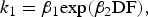 $$k_1 = \beta _1 {\rm exp(}\beta _2 {\rm DF),}$$
 $$k_2 = \beta _3 + \beta _4{\rm exp(}\beta _5{\rm DF)},$$
where β i are the fitted coefficients. The corresponding on-glacier temperature T 1 was calculated as T*·k 1 (Shea and Moore, Reference Shea and Moore2010). The original fitted parameters were found to model T a well across La Mare Glacier in the Ortles-Cevedale range, Italy (Carturan and others, Reference Carturan, Cazorzi, De Blasi and Dalla Fontana2015). Here we apply the original parameters of Shea and Moore (Reference Shea and Moore2010), referred to as SM10, and the parameters (k 1 and k 2) fitted to the data for centreline stations on Tsanteleina Glacier, referred to as SMopt.
The modified form of the thermodynamic model (Greuell and Böhm, Reference Greuell and Böhm1998), referred to as ModGB, follows the form:
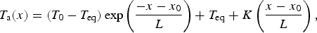 $$T_{\rm a} (x) = (T_0 - T_{{\rm eq}} )\,{\rm exp}\left( {\displaystyle{{ - x - x_0} \over L}} \right) + T_{{\rm eq}} + K\left( {\displaystyle{{x - x_0} \over L}} \right),$$
where T 0 (°C) is the air temperature at the theoretical location where air enters the KBL x 0 (selected by visual inspection of the mid accumulation area following Ayala and others, Reference Ayala, Pellicciotti and Shea2015). T 0 is also derived from extrapolated T a using the GCELR method (Table 2). T eq is the ‘equilibrium temperature’ and L (metres) is the length scale. The original form of the model (Greuell and Böhm, Reference Greuell and Böhm1998) attempts to explain down-glacier cooling within the KBL, while last term was introduced by Ayala and others (Reference Ayala, Pellicciotti and Shea2015) to account for observed warming on glacier tongues with an empirical factor K (°C). L is calculated according to the original study of Greuell and Böhm (Reference Greuell and Böhm1998) by:
 $$L = \displaystyle{{H\,\cos {\rm (}a{\rm )}} \over {B_{\rm H}}}, $$
where H is the height of the boundary layer (m), B H represents the bulk transfer coefficient for heat and a is the mean glacier slope (°). T eq is derived from:
 $$T_{{\rm eq}} = bL,$$
where b is calculated using the dry adiabatic lapse rate Γ d by:
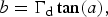 $$b = \Gamma _{\rm d} \tan (a),$$
Following Ayala and others (Reference Ayala, Pellicciotti and Shea2015), H and K are used as tuning parameters when fitting the model to observations of T a along the glacier centreline during warm ambient conditions. The derivation of the original thermodynamic model is explained in detail in Greuell and Böhm (Reference Greuell and Böhm1998) and not repeated here. Ayala and others (Reference Ayala, Pellicciotti and Shea2015) suggest that the original model (of Greuell and Böhm, Reference Greuell and Böhm1998) is not applicable to small glaciers with a short fetch. As such, the original model form is not included in the analysis of Tsanteleina Glacier. SM and ModGB parameters for Tsanteleina Glacier are derived from all available data for the combined Jul–Aug and Aug–Sep periods and used to distribute temperature in the separate periods for melt modelling (see Melt modelling section).
As an input to an energy-balance model, ModGB is applied only for T 0 temperatures ≥6°C, where parameters begin to converge for previously studied glaciers (Ayala and others, Reference Ayala, Pellicciotti and Shea2015, Reference Ayala, Pellicciotti, Peleg and Burlando2017). These studies have shown that on-glacier temperatures are well reproduced by linear gradients below this T 0 threshold, and we thus apply GCELR (Table 2) for T 0 < 6°C.
4.4. Melt modelling
The importance of different methods of air temperature distribution to melt model calculations is assessed through their application in a physically based energy-balance model (Reid and others, Reference Reid, Carenzo, Pellicciotti and Brock2012) applied at distributed stake locations on Tsanteleina Glacier. Melt (M) is calculated for the given time step (∆t) by:
 $$M = \displaystyle{{Q_{\rm m} \Delta t} \over {\,p_{\rm w} L_{\rm f}}}, $$
where L f is latent heat of fusion (J kg−1), p w is the density of water (kg m−3) and Q m is the energy available for melt, calculated as:
 $$Q_{\rm m} = S_{{\rm net}} + L_{{\rm net}} + H + L_{\rm E} + P + G,$$
where S net and L net are the net fluxes of shortwave and longwave radiation, respectively, H and L E are the turbulent fluxes of sensible and latent heat, P is the heat flux provided by rain and G is the conductive heat flux into the snow or ice. Model calculations were performed on a 30 m gridcell size, consistent with the available ASTER GDEM resolution.
Wind speed and relative humidity were treated as spatially constant values from the LWS (UWS) below (above) 3100 m a.s.l. in order to treat the upper and lower glaciers with the most locally available data. Summer snow accumulation was estimated at each site using precipitation data at CH (Fig. 1), a precipitation gradient of 0.0026 mm h−1 m−1 (Fyffe and others, Reference Fyffe2014) and a liquid precipitation threshold of 1°C (Jóhannesson and others, Reference Jóhannesson, Sigurðsson, Laumann and Kennett1995; MacDougall and others, Reference MacDougall, Wheler and Flowers2011). Snow accumulation was negligible during Jul–Aug, but contributed a total of 0.28 m w.e. to the LWS site during Aug–Sep (Fig. 2e).
Binary grids were created utilising the hill shade algorithm in ArcGIS (Shaw and others, Reference Shaw2016) to identify shaded glacier cells at each time step. The proportions of direct and diffuse radiation recorded at LWS were calculated and distributed across glacier accounting for cell slope and aspect using the equations in Brock and Arnold (Reference Brock and Arnold2000) and a sun position algorithm (Reda and Andreas, Reference Reda and Andreas2008). Surface roughness (z 0) was calculated at 14 locations across the whole glacier in July 2015 using the microtopographic method (Munro, Reference Munro1989; Brock and others, Reference Brock, Willis and Sharp2006) and interpolated using inverse distance weighting. The obtained values lie within the range of the literature (see Brock and others, Reference Brock, Willis and Sharp2006) and vary from 2 mm (smooth ice) to 16 mm (crevasse fields).
4.5. Evaluation of temperature distribution models
Model performance and the effectiveness of the different temperature distribution methods are evaluated by comparing measured melt rates at centreline and lateral sites (which have stake data in both periods) to modelled melt from the different T a distribution methods outlined in Table 2. Modelled melt rates are also compared to a reference model using measured air temperature and assessed with respect to the potential manufacturer errors in the temperature input data. T a values are varied ±0.35°C (the maximum error range for the TinyTag loggers) uniformly across all input data prior to the reference model run and compared to the melt estimation from the different temperature distribution methods.
5. RESULTS: OBSERVED TEMPERATURE VARIABILITY
5.1. Temperature variability under different meteorological conditions
Mean station T a values conform to an approximate linear relationship with elevation, particularly when only considering the centreline stations (Fig. 3). Table 3 shows the mean VTGs for all subsets of time and meteorological conditions. Mean VTGs for all subsets are similar to, or more negative than the ELR, with the exception of high off-glacier temperatures (90th percentile, see Methodology section). This is particularly the case during Aug–Sep, when the on-glacier temperature distribution can no longer be explained by elevation (low, non-significant R 2 values in Table 3). In contrast, under the coldest off-glacier temperatures (tenth percentile, typically clear nights), VTGs become very steep and a strong relationship to elevation is evident.
Mean T a-elevation relationships for all stations (upper panels) and centreline stations only (lower panels). The circles indicate mean T a (green), and the means of the 90th (red) and tenth (blue) percentiles of off-glacier temperatures at Grand Croux (GC) station. The shaded area represents one SD (this is larger for the green plots as they represent all data). Data for TE11–13 are not shown for Aug–Sep due to larger data gaps. Sites investigated as cold spots (Fig. 4) are shown by the filled circles. Their elevation information is given in Table 1.

The difference in measured T a at three lateral sites (TE0, TE6 and TE12) and one centreline site (TE3) from T a estimated by VTGCL (x-axis), plotted against wind speed at LWS (UWS for TE12) (y-axis) and mean sea-level pressure (colour scale) derived from the ERA-interim reanalysis dataset (http://apps.ecmwf.int/datasets/data/interim-full-daily/levtype=sfc/). Reanalysis data were linearly interpolated from 6-hourly to hourly intervals to correspond with hourly data for Tsanteleina. Negative x-axis values indicate that station temperatures are cooler than the corresponding elevation on the centreline.

Vertical temperature gradients (VTG) derived from linear regression of temperature observations against elevation for all available on-glacier data in each period and for different conditions
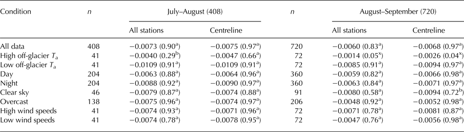
VTGs are reported in °C m−1 with R 2 (coefficient of determination) values in parentheses for means of all stations (including lateral stations) and centreline stations only
aIndicates where the R 2 relationship is statistically significant to the 99% level, bwhere it is significant at the 95% level and xwhere it is not statistically significant.
Generally, night-time VTGs are steeper than daytime, particularly in Jul–Aug; although day/night differences are less distinct in general than between high- and low-temperature conditions (Table 3). Overcast conditions had little effect on VTG magnitude compared with clear sky conditions in Jul–Aug, but were associated with much less negative VTGs in Aug–Sep. Elevation dependency of T a is strong (high R 2 values) for overcast conditions in both periods.
5.2. Lateral and centreline anomalies
As shown in Table 3, elevation becomes a poorer predictor of T a when lateral stations are included, evident from the reduction in R 2 (coefficient of determination) for all stations in both periods. Furthermore, for the warmest conditions, cross-glacier T a variability is greatest (Figs 3a, b).
Lateral sites TE0, TE6 and TE12 (Fig. 1) frequently exhibited lower T a than expected when compared with centreline temperatures for the same elevations (Fig. 3). Furthermore, centreline site TE3 also exhibited notably cooler temperatures during both periods than its elevation would suggest (these stations are indicated by filled circles in Fig. 3). Hourly temperature deviations at these sites were quantified by comparison with the centreline temperatures estimated for their elevations, based on VTGCL (Table 2).
Hourly T a depressions at these sites are largest at relatively low, but not calm, wind speeds of 2–3 m s−1 (derived from the nearest weather station) under warm, high-pressure conditions (Fig. 4). During periods of low-pressure and high synoptically forced wind speeds, differences from the centreline T a are very small, particularly for TE0 and TE6. This feature is less consistent for sites TE3 and TE12, which also show several hours of positive temperature anomaly for moderately high pressure and low-to-moderate wind speeds. The lowest 10% of wind speed values (≤1 m s−1) resulted in less negative (though significant) VTGs in Aug–Sep, though wind speed percentiles show no clear differences in elevation dependency or slope of VTGs for Jul–Aug (Table 3).
6. RESULTS: TEMPERATURE ESTIMATION
6.1. Off-glacier VTGs
The VTG between the two off-glacier stations CH and GC fluctuates between strong negative (<−0.0100 °C m−1) gradients to moderate inversions (up to +0.0031 °C m−1) over their large elevation difference (>900 m – Fig. 5). Due to the position of the CH in Val di Rhêmes, cold air which sinks into the valley during the night results in a frequent inversion layer whereby the GC station is warmer. This reiterates the suggestions of Oerlemans (Reference Oerlemans2001) and Carturan and others (Reference Carturan, Cazorzi, De Blasi and Dalla Fontana2015) that high-altitude stations are preferable to those within valleys for distributing air temperature.
Boxplots of hourly VTGs for (a) centreline stations (VTGCL) and (b) between off-glacier stations Chaudanne (1794 m a.s.l.) and Grand Groux (2750 m a.s.l.) in both periods. Boxplot limits show the 25th and 75th percentiles and outliers are shown by the red crosses.
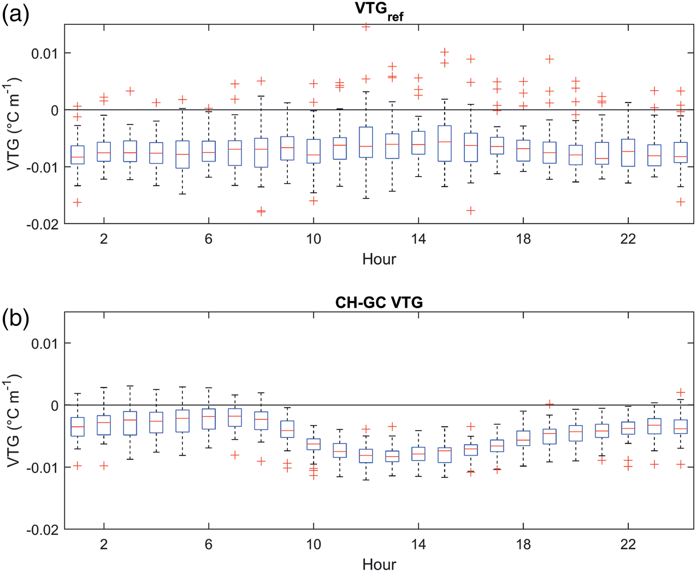
The mean diurnal variation of the off-glacier VTG is generally the inverse of that of the glacier centreline, though with less variance (Fig. 5). During the day, VTGs along the glacier centreline (VTGCL) are relatively shallow, especially for warm, high-pressure conditions where a KBL begins to develop. In contrast, off-glacier VTGs become more negative due to stronger warming at CH. However, at night, the tendency towards inversions for the off-glacier data contrasts with more negative gradients for the glacier centreline (Fig. 5 and Table 3). The mean VTG for the off-glacier stations is −0.0047 °C m−1 for the combined periods. The application of the off-glacier VTG (GCoff) or ELR (GCELR) overestimates on-glacier temperature by up to 1.5°C on average (Fig. 6a). For the warmest ambient conditions, this overestimation can be as high as 4°C for GCELR (Fig. 6b) leading to an RMSE of 3.6°C compared to the measured data.
Measured centreline T a (red) and estimation of T a for the mean of all hours (a, c, e) and the mean of the warmest T 0 bin (12–13°C, n = 12) (b, d, f). Panels a and b show the estimation of T a using extrapolation with the off-glacier VTG (GCoff – blue) and the ELR (GCELR – green) from the Grand Croux station (red star). Panels c and d show estimated T a when applying Shea and Moore with original parameters (SM10 – blue) and recalibrated parameters (SMopt – green). Panels e and f show estimated T a with the modified Greuell and Böhm model (ModGB – green), together with VTGCL (blue). RMSE values (°C) represent the fit of each method to the mean measured data.

The mean cooling effect (mean error) and RMSE between measured and estimated temperature at each station is given in Table 4. The mean cooling effect of all lateral stations using GCELR is −1.43°C, compared with −1.12°C for centreline stations (Table 4). Although the difference in mean cooling effect between sites for the whole period is not largely different from the measurement error of the sensors, the main differences are found in the warmest conditions (Figs 3, 4).
The mean ‘cooling effect’ (MCE) and root mean square error (RMSE) of the fit to measured data for the centreline (top half) and lateral sites (bottom half) from extrapolated temperatures using GCELR, SM10, SMopt and ModGB (Table 2)
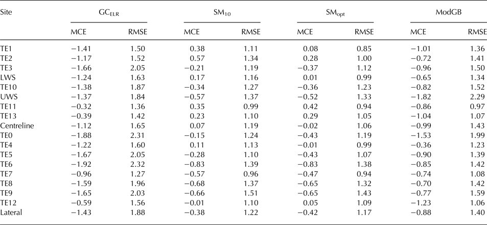
The MCE is calculated as measured T a−estimated T a. MCE and RMSE are expressed in °C. The mean of all centreline and lateral sites are also given.
6.2. SM approach
The SM approach using the original (SM10) and optimised (SMopt) coefficients estimates mean T a along the centreline of Tsanteleina Glacier well (Fig. 6c). For the mean of all conditions in both periods, the SM approach performs worse than using GCELR or GCoff (RMSE difference of 0.40 and 0.36°C for SM10 and SMopt, respectively, compared with GCELR – Figs 6a vs c). However, for the warmest conditions at the top of the glacier flowline (T 0 = 12–13°C), the application of the SM model offers a clear improvement over GCELR (Figs 6b vs d).
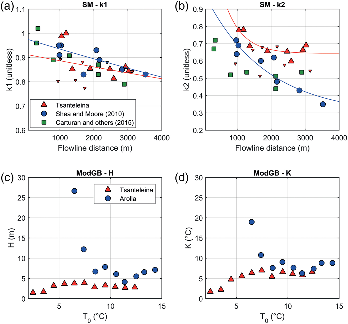
However, the exponential parameterisation of k 2 from SM10 (blue line in Fig. 7b) does not suitably describe the cooling of T a above the threshold for katabatic onset and thus cannot replicate the warmer T a on the glacier tongue for the highest ambient temperatures (Fig. 6d). Although lateral observations on Tsanteleina Glacier appear to be less sensitive to ambient temperatures at greater flowline distances (small triangles in Fig. 7b), centreline k 2 parameters stabilise at ~2000 m along the flowline and are not replicated by the exponential equation provided by SM10. The k 1 parameter, however, is less variable for centreline and lateral stations compared with the k 2 parameter and similar to the values from the literature (Fig. 7a – Shea, Reference Shea2010; Carturan and others, Reference Carturan, Cazorzi, De Blasi and Dalla Fontana2015). The original and optimised coefficients (Eqns (3) and (4)) are provided in Table 5.
Parameter values for the Tsanteleina dataset for the Shea and Moore method (SM) (a and b) and the modified Greuell and Böhm (ModGB) (c and d) compared with the parameter values from the published literature. k 1 (a) and k 2 (b) parameters are presented for Tsanteleina (red triangles – small triangles for lateral stations), the study sites of Shea and Moore (Reference Shea and Moore2010) (blue circles) and of Carturan and others (Reference Carturan, Cazorzi, De Blasi and Dalla Fontana2015) (green squares). The parameterisations in Eqns (2) and (3) are shown for SM10 and SMopt by the blue and red lines, respectively. ModGB parameters H (c) and K (d) are plotted as functions of T 0 for Tsanteleina Glacier (red triangles) and Arolla Glacier (blue circles). Upper panels are cropped and do not show a parameter of Shea and Moore (Reference Shea and Moore2010) at ~10 000 m flowline distance.
The parameter/coefficient set for the boundary layer models SM and ModGB as given for the current dataset and as published in the literature
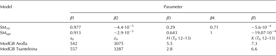
Parameters for the SM model are taken from Shea (Reference Shea2010) and ModGB values for Arolla Glacier are taken from Ayala and others (Reference Ayala, Pellicciotti and Shea2015). The β coefficients from Shea and Moore (Reference Shea and Moore2010) are originally β3–7 (for parameters k 1 and k 2).
SMopt estimates T a better at centreline locations such as TE10 than at lateral sites at similar flowline distances (e.g. TE9 – Table 4). The improvement over the use of SM10 is more noteworthy for centreline sites, though SMopt consistently has the lowest RMSE between the measured and estimated temperatures as the k 1 and k 2 parameters are fitted to the station data for the glacier (Figs 7a, b). Lateral stations have a higher RMSE on average for SMopt than centreline stations though they show the largest average improvement in RMSE compared to GCELR (Table 4).
6.3. Application of ModGB
Under warm ambient temperatures (temperature at T 0 ≥ 6°C), ModGB is able to replicate the initial down-glacier cooling effect and warming on the glacier tongue (Figs 6e, f). Fitted parameters H and K are ~2–3 m and 6–7°C, respectively, for T 0 ≥ 6°C, smaller and more stable values than those found by Ayala and others (Reference Ayala, Pellicciotti and Shea2015) for Arolla Glacier (Table 5, Figs 7c, d).
For comparison with ModGB, all methods of T a distribution are binned into T 0 intervals to assess their performance at replicating on-glacier temperature (Fig. 8). The ModGB approach better fits to the mean measured centreline data than the other temperature distribution methods (based on RMSE) for all T 0 bins. Compared with GCELR, the SM approaches and ModGB are both superior because the cooling effect of the glacier surface is accounted for, even when including lateral T a variability (crosses in Fig. 8a). For cooler ambient conditions (e.g. T 0 = 2–5°C), the application of GCELR is more appropriate for representing on-glacier temperatures, but is still out-performed by the on-glacier T a distribution models. Even compared with VTGCL, ModGB has a lower RMSE for the warmest ambient conditions (Fig. 8b). This is, however, the result of inappropriate fitting of the ModGB equation when the air temperature is more linear with elevation (Fig. 6e). In a time-series application, ModGB reduces error compared to GCELR, but is out-performed in modelling hourly T a by the SM approaches (Table 4). The suitability of extracted parameters is an important consideration for the ModGB approach which is addressed in the Discussion section.
Calculated RMSE (°C) of measured T a and estimated T a using GCELR, SM10, SMopt and ModGB for T 0 bins (panel a). Panel b shows the same ModGB performance relative to the RMSE of VTGCL as a function of T 0 bins. RMSE calculated using the measured mean data for centreline stations and all stations (‘lateral’) for each T 0 bin.

Model errors are greater when ModGB is assessed against all T a data (including non-centreline) for all ambient temperature ranges (RMSE of 1.1°C for T 0 = 12–13°C, red crosses in Fig. 8). However, ModGB is not, by definition, designed to account for marginal temperature variability. Furthermore, the SMopt method (Fig. 8a) or VTGCL (Fig. 8b) also lead to a high RMSE of 1.17 and 0.99°C, respectively, for T 0 = 12–13°C and much of the variability in lateral T a under warm ambient conditions is also poorly estimated.
7. RESULTS: MELT MODELLING
7.1. Validation of melt models
‘Reference model’ melt values are provided by running the energy-balance model using meteorological inputs as described in the Methods section and measured on-glacier T a at each T-logger/AWS site (Fig. 9). There is a tendency towards model underestimation in Jul–Aug and overestimation in Aug–Sep, but RMSEs of 0.0030 m w.e. d−1 in Jul–Aug and 0.0034 m w.e. d−1 in Aug–Sep are acceptable given potential error sources in both model and data (error bars in Fig. 9). Notably, reference model melt and stake ablation agree very well at LWS in both periods, suggesting extrapolation of meteorological input variables and glacier parameters accounts for at least some of the scatter between model and data. Distribution of wind is a possible cause of strong melt overestimation at TE5 and TE6 in both periods (circled) which are considered to be topographically sheltered areas of the glacier (see Discussion section). Measured daily average melt range from 0.048 to 0.059 m w.e. d−1 for Jul–Aug and 0.030 to 0.038 m w.e. d−1 for Aug–Sep.
Reference measured vs modelled average daily ablation (m w.e. d−1) for all stake data in Jul–Aug (red) and Aug–Sep (blue) with the RMSE for the fit in each period. An error range of 5 cm (Reid and others, Reference Reid, Carenzo, Pellicciotti and Brock2012) for each period is shown by the horizontal error bars (averaged over the number of days). Vertical error bars indicate the uncertainty associated with a uniform air temperature perturbation of ±0.35°C. The dashed circles indicate sites of consistent model overestimation associated with calm wind flow (see text).

7.2. Distributed temperature and modelled melt rates
Figure 10 shows the daily mean melt rates for model runs with the distribution of T a using VTGs, ModGB or SM approaches. These results (solid coloured circles) are compared with measured stake data and reference model runs as in Figure 9 (hollow black circles and error bars). The RMSE and bias of all model runs are shown in Table 6.
Measured and modelled daily average melt (m w.e. d−1) at stake sites using different T a distribution methods (see Table 2). Data are shown for selected centreline and lateral sites with observations in both Jul–Aug (red) and Aug–Sep (blue) (see Fig. 9). Horizontal error bars indicate a 5 cm error for measured ablation and vertical error bars indicate the uncertainty associated with a uniform air temperature perturbation of ±0.35°C in the reference model. RMSE and mean bias values are reported in m w.e. d−1 for each model run/period. Panel c shows the performance of ModGB if applied to all T 0 temperatures ≥2°C. Metrics of all model runs are shown in Table 6.

RMSE and mean bias of melt model results for the different temperature distribution methods (reported in m w.e. d−1)
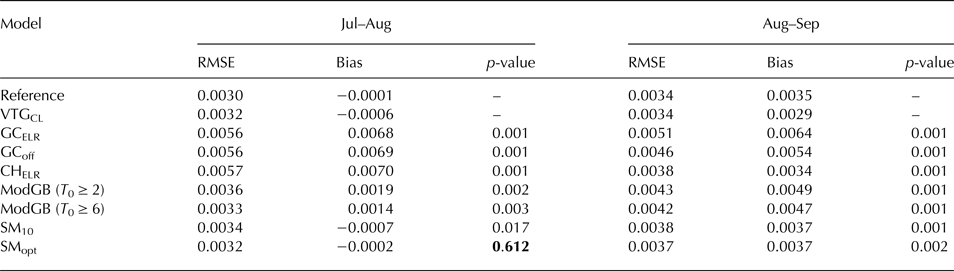
P-values indicate the results of a Wilcoxon rank-sum test of the statistical differences in the median RMSE between the reference model results at all stakes and different T a distribution methods compared to the use of an on-glacier VTG (VTGCL). The reported p-values indicate the statistically significant differences compared to VTGCL at the 95% level for Jul–Aug and Aug–Sep. Where p > 0.05, the method does not perform significantly different to the use of on-glacier data and a local VTG (these instances are shown in bold).
VTGCL provides a good fit to the measured melt rates at stake locations (RMSE = 0.0032 m w.e. d−1 in Jul–Aug) as it represents the on-glacier recorded T a at LWS and a VTG calculated from several on-glacier T-loggers (Fig. 5 upper panel, Fig. 10a). T a extrapolation from off-glacier sites using VTGs results in model overestimation (a positive bias). For example, melt at LWS is overestimated by ~0.006–0.010 m w.e. d−1 using all three VTG methods during Jul–Aug (Table 6). This overestimation of the melt is shown for GCELR in Figure 10b.
SM10 is found to underestimate melt rates at many sites compared to the reference run (negative bias), particularly at lower elevations/greater flowline distances (Fig. 10e). The application of SMopt provides improved melt model performance compared to SM10, though still underestimates the reference model melt rate at some stations (Fig. 10f). For lateral sites TE5 and TE6, SMopt performs similarly to the reference. Performance of SM10 and SMopt is very similar for the cooler Aug–Sep period.
The application of ModGB for T 0 ≥ 6°C (the convergence of H/K in the literature – Ayala and others, Reference Ayala, Pellicciotti and Shea2015, Reference Ayala, Pellicciotti, Peleg and Burlando2017) resulted in an RMSE reduction of 0.0023 m w.e. d−1 compared with an off-glacier VTG distribution (Fig. 10d), in spite of only ~35% of the total time steps at T 0 being ≥6°C, and T a was otherwise distributed using a GCELR approach. As H and K parameters are stable for all T 0 ranges on Tsanteleina Glacier (Figs 7c, d), ModGB was also run for T 0 ≥ 2°C. However, as this method is designed for warm ambient temperatures, reducing this threshold implies a too greater warming effect on the glacier tongue for cooler ambient temperatures and melt rates are overestimated at TE2 (Fig. 10c). Applying ModGB for T 0 ≥ 2°C nevertheless improved estimates of melt compared to GCELR.
The use of the SM and ModGB temperature distribution methods improves modelled melt rates by an RMSE of between 0.0020 and 0.0024 m w.e. d−1 (28–36% RMSE reduction) compared to GCELR, though only SMopt is statistically similar to the on-glacier VTGCL distribution when compared to the reference model using a Wilcoxon ranked-sum test (Table 6). In the context of model errors, both ModGB (for T 0 ≥ 6°C) and the SM approaches are within the maximum uncertainty of T a records assuming a uniform ±0.35°C air temperature perturbation.
8. DISCUSSION
8.1. Temperature distribution and VTGs
The weak dependence of centreline temperature on elevation under warm ambient conditions recorded at Tsanteleina Glacier concurs with the majority of previous findings regarding katabatic effects on T a distribution (e.g. Greuell and Böhm, Reference Greuell and Böhm1998; Shea and Moore, Reference Shea and Moore2010; Petersen and others, Reference Petersen, Pellicciotti, Juszak, Carenzo and Brock2013; Ayala and others, Reference Ayala, Pellicciotti and Shea2015). However, on-glacier VTGs were on average more negative than found in previous studies (e.g. Strasser and others, Reference Strasser2004; Carenzo, Reference Carenzo2012; Marshall, Reference Marshall2014). Tsanteleina Glacier likely has a thin boundary layer due to its small size, and a katabatic flow influence on centreline T a distribution only dominates for high ambient temperatures (Fig. 6f, Table 3). Carturan and others (Reference Carturan, Cazorzi, De Blasi and Dalla Fontana2015) also derived gradients that are steeper than the ELR over a small glacier with a similar northeast orientation (La Mare Glacier) to Tsanteleina Glacier. They attributed this in part to station positioning and the presence of steeper slopes above a lower station, which resulted in the dominance of adiabatic heating under compression (Greuell and others, Reference Greuell, Knap and Smeets1997; Greuell and Böhm, Reference Greuell and Böhm1998, Strasser and others, Reference Strasser2004). On Tsanteleina Glacier, the strong negative VTGs derived by regression of multiple stations with elevation (Fig. 3) would not be strongly influenced by such site-specific factors, however. Although VTGCL poorly accounts for the structure of on-glacier T a variability under the warmest conditions, it still performs well at modelling daily average melt rates relative to the reference model (Fig. 10a). However, as both on-glacier data and locally-derived VTG would typically be unavailable for regional and larger scale studies over unmonitored glaciers, it is important that the temperature distribution models using off-glacier T a be applied with generalisable parameters and thresholds.
For warm ambient conditions (where top-of-flowline temperatures exceed 6°C), the application of an off-glacier VTG was found to be unsuitable for estimating on-glacier temperature. This is because off-glacier stations are (a) outside the influence of the glacier boundary layer and (b) affected by local topographic influences on temperature, e.g. shading, cold air drainage. Several previous studies have found similar issues with off-glacier temperature extrapolation (Shea and Moore, Reference Shea and Moore2010; Carturan and others, Reference Carturan, Cazorzi, De Blasi and Dalla Fontana2015). Hence, alternative parameterisations or corrections for T a distribution are required to distribute on-glacier temperatures. It is difficult to determine what off-glacier sites are truly ‘representative’ and suitable for extrapolation of temperature to the elevation of the glacier. Exploratory analyses revealed that deriving temperature gradients between a series of local stations at higher elevations than CH in the neighbouring valleys produced similarly shallow VTGs, mostly likely due to topographically induced air circulation patterns and their effects on valley sites. Therefore, the initial temperatures (T 0 and T amb) of the boundary layer temperature estimation methods were extrapolated from GC using the ELR.
8.2. Application of on-glacier temperature distribution models
In this study, T* from the SM method was parameterised as a function of the flowline distance (Eqn (2)) following Carturan and others (Reference Carturan, Cazorzi, De Blasi and Dalla Fontana2015) because the original method (as a linear function of elevation (Shea and Moore, Reference Shea and Moore2010)) resulted in low T* values across the glacier (3.1–3.8°C). In the original SM10 model, values of the k 2 parameter decrease continuously with increasing flowline distance, whereas k 2 parameter values derived from the Tsanteleina data are higher for equivalent flowline distances and level off beyond 2000 m (Fig. 7b). Such marked spatial variation in the k 2 parameter means that the SM approach requires further evaluation and development to account for local effects on KBL development before it can be applied generally. The levelling-off of k 2 parameter values at short flowline distances in both this study and Carturan and others (Reference Carturan, Cazorzi, De Blasi and Dalla Fontana2015) (green triangles in Fig. 7b) suggests that, for small glaciers, the continued down-glacier cooling effect may be generally absent (Fig. 6d). This is particularly the case for the occurrence of warmer temperatures on the tongue of Tsanteleina Glacier which are better modelled by the ModGB approach. It is perhaps unlikely that the SMopt parameterisation (red line in Fig. 7b) will be transferable to other glacier sites, though it emphasises the requirement for more distributed datasets to calibrate a globally applicable parameter set which may act as a function of glacier size. Over larger flowline distances, it has been suggested that the development of the KBL is sufficient to minimise the influence of free-atmospheric temperatures and that the coolest on-glacier temperatures are experienced at the glacier terminus (Greuell and Böhm, Reference Greuell and Böhm1998; Shea and Moore, Reference Shea and Moore2010). In this instance, SMopt still underestimates melt at some sites (Fig. 10), though provides an improved fit (RMSE) to the data compared with SM10.
ModGB had the lowest RMSE of all the temperature distribution methods (Fig. 8) as well as a linear on-glacier VTG (Figs 6e, f) when estimating mean T a for most T 0 bins. The parameters H and K were smaller than those obtained for Arolla Glacier (Figs 7c, d), likely due to the glacier's size which has insufficient fetch to create a strong KBL and lacks length to sustain it. Of local significance to Tsanteleina Glacier is the fact that the dominant synoptic wind direction from the west is aligned with the down-glacier flow at LWS. Identifying a clear switch between katabatic conditions and erosion by synoptic-scale events is therefore difficult. Nevertheless, during periods of strong, synoptically driven winds, temperature gradients were highly linear and negative (Table 3) and lateral differences reduced because of the lack of identified glacier ‘cold spots’ (Fig. 4).
In general, ModGB appears to be a useful tool for explaining along-flowline T a variability that has a physical basis. The development of this thermodynamic approach has led to improvements in RMSE compared to off-glacier or on-glacier VTGs (Greuell and Böhm, Reference Greuell and Böhm1998; Petersen and others, Reference Petersen, Pellicciotti, Juszak, Carenzo and Brock2013; Ayala and others, Reference Ayala, Pellicciotti and Shea2015; Carturan and others, Reference Carturan, Cazorzi, De Blasi and Dalla Fontana2015). Nevertheless, as a practical solution to modelling glacier melt rates; there remains a continued uncertainty about the threshold conditions for the implementation of ModGB that needs to be further explored. For example, as the H and K parameters are calibrated for warm ambient temperatures (Figs 7c, d), they are unsuitable for cool conditions (suggestions from Arolla Glacier (Ayala and others, Reference Ayala, Pellicciotti and Shea2015) and Juncal Norte Glacier, Chile (Ayala and others, Reference Ayala, Pellicciotti, Peleg and Burlando2017)), and therefore a threshold for the application of ModGB is required. In this respect, although the ModGB performs better than the SM approach at explaining mean conditions as a function of T 0 temperatures when it is fitted to the data (Figs 6, 8), it is outperformed by the SM approach in estimating individual hourly temperatures (Table 4) and melt rates (Fig. 10d) at individual stations, particularly at lateral locations. This is largely the result of the poor estimation of T a for hours below the temperature threshold, which is still estimated by GCELR. Applying ModGB above a lower threshold (2°C) inadequately represented hourly temperatures and melt rates on the lower glacier (Fig. 10c) and demonstrates that appropriate thresholds are important. Although both ModGB (for T 0 ≥ 6°C) and SM methods modelled daily average melt within the maximum uncertainty of the temperature sensors (Fig. 10), they require further development before large-scale deployment in regional glacier studies.
A constraint for the distribution of T a using SM and ModGB is that they are designed to only account for T a changes along a glacier centreline where katabatic conditions are theoretically strongest. These methods likely cannot represent mean measured data at lateral station locations due to the fact that these sites can be affected by advection of warm air from surrounding topography (e.g. TE4 – Hannah and others, Reference Hannah, Gurnell and McGregor2000), localised cooling (Fig. 4) or that sensible and latent heat exchanges can be reduced near to glacier margins outside the influence of the KBL (Shea and Moore, Reference Shea and Moore2010). Estimation of temperatures using the SM approach is worse on average for lateral locations compared with centreline stations (Table 4), though the performance of most approaches is not clearly superior at centreline locations in the results of an energy-balance model (Fig. 10).
The selection of the most appropriate model for estimating T a over mountain glaciers could be considered with respect to the number of parameters and the amount of fitting to large datasets it requires. The SM approach has eight unknowns (β1–5, C1–2 and the value of the VTG used to extrapolate initial temperature) and ModGB has four (H, K, x 0 and the off-glacier VTG). Although direct comparison of method performance based on parameter quantity is not feasible with such different approaches, the lower RMSE of the SM methodology for estimating hourly temperatures could be argued to be related to its reliance on double the number of parameters that ModGB requires. Nevertheless, as is evident from the inappropriate fitting of ModGB to data for cooler conditions (Figs 6e, 8), its application necessitates a further threshold value which is also sensitive to the location and elevation of the point where air enters the KBL (x 0). Further still, it is found that the stability of extracted parameters H and K may vary between different sites (Figs 7c, d), and so the threshold conditions for application of ModGB may be more necessary in certain cases than others. Crucially, the exact processes causing warmer air temperatures on glacier tongues is still uncertain (e.g. Sauter and Galos, Reference Sauter and Galos2016), and so selecting the optimum method for distributing air temperatures in long-term glacier melt models remains unclear. The ModGB approach has clear advantages for calculation of air temperature for the warmest conditions on Tsanteleina Glacier, but when utilised for calculation of melt rates, its performance decreases because it relies on the accuracy of an off-glacier gradient below the threshold temperature. Because of its physical basis, the derivation of parameters (such as the height of the boundary layer, H) may be afforded by other datasets such as tower measurements or radiosondes (Greuell and Böhm, Reference Greuell and Böhm1998). Alternatively, the parameterisation suggested by Shea and Moore (Reference Shea and Moore2010), though potentially more generally applicable, is only statistical in nature and currently does not account for the warming on glacier tongues.
A final consideration is the sensitivity of these methods to different temperature extrapolation from the off-glacier site GC. As the local VTG is a generally unknown value (as stated above), the current boundary layer models have been forced with high elevation T a and the ELR (−0.0065 °C m−1). However, high variability in locally derived off-glacier VTGs (Fig. 5) will introduce uncertainty and this needs to be further addressed as such boundary layer models become more generalisable and require initial temperature forcing data.
8.3. Glacier ‘cold spots’ and distributed wind speed
Sites TE0, TE3, TE6 and TE12 exhibited consistently colder T a relative to sites at similar elevations or flowline distances on the glacier for warm ambient conditions (Fig. 3). These ‘cold spots’ at TE6 and TE12 are hypothesised to be due to topographic depressions in the glacier surface which promote the entrapment of radiatively cooled stagnant air under calm, high-pressure conditions (Fig. 4). Topographic depressions coincident with the sites of TE6 and TE12 can be inferred from analysis using GIS hydrology ‘sink’ tools (results not shown) but the available ASTER DEM is of too coarse resolution (30 m) to provide a robust test of this hypothesis. Differences in modelled global radiation at lateral and centreline sites were small (<10 W m−2 on average between TE6 and LWS) and the intercomparison tests (see Supplementary Material) found that the naturally ventilated T a measurements were not noticeably affected by moderately low wind speed conditions in the presence of insolation, lending support to the legitimacy of these observations.
Less clear is the cause of low-temperature anomalies at centreline site TE3, which occurred under both high and low wind speeds (Fig. 4). Temperatures along this part of the flowline are, however, consistent with findings of Foessel (Reference Foessel1974) and Munro (Reference Munro2006) who explain ‘cold spots’ from the convergence of tributary air flows on Peyto Glacier, Canada. Convergence of air at LWS and TE3 from the southern limb of Tsanteleina Glacier (Fig. 1) could increase the boundary layer thickness and limit the entrainment of warmer free air (Munro, Reference Munro2006), thus accounting for cooling at TE3 (also during windier conditions). Furthermore, the pattern of anomalies of T a at TE0 was similar to that found at TE6 (Fig. 4), though differences in modelled radiation were very small. TE0 was considered as a lateral site for this investigation, though its distance from TE1 (with warmer observations of T a) is only ~100 m. This raises questions about the processes influencing near-surface air temperatures at different locations on the glacier tongue and how well they are represented by either VTGs or alternative models tested in this study.
Overestimation of wind speed at TE6 and TE5 is a possible reason for overestimation of melt rate when using the locally measured T a (Fig. 9). Artificially halving the wind speed in the melt model at these locations results in a close match to measured melt rates. Following the method proposed by Winstral and others (Reference Winstral, Elder and Davis2002), the exposure of different model gridcells across the glacier was determined using wind direction measured at both AWS sites and the elevation information from the DEM (results not shown). While this is a crude approach given the DEM resolution, both TE6 and TE5 (as well as TE12 – Fig. 4) are suggested to be sheltered from the dominant westerly wind direction by the surrounding topography and lower wind speeds at these sites are potentially likely. Modelling distributed wind fields across glaciers remain problematic and an area for future research beyond the scope of this paper.
9. CONCLUSIONS
This study has analysed a network of centreline and lateral air temperature observations over an alpine glacier during the 2015 summer ablation season. Two recently published methods from the literature that attempt to reproduce the cooling of air temperature over a melting glacier were tested and applied to an energy-balance model. The key findings of this work are:
-
(1) When top-of-flowline ambient air temperatures are low (<6°C), VTGs (e.g. the linear variation of temperature with elevation) can reproduce temperature variability. However, when ambient temperatures are high (>6°C), on-glacier air temperatures are only weakly dependent on elevation and a VTG is inappropriate for its estimation, particularly when extrapolated from an off-glacier location that does not account for the glacier cooling effect.
-
(2) The two alternative methods proposed in the literature by Shea and Moore (Reference Shea and Moore2010) and Ayala and others (Reference Ayala, Pellicciotti and Shea2015) improve estimates of on-glacier air temperature for warm ambient conditions compared with the use of off-glacier temperature gradients, because they account for the glacier cooling effect (RMSE reduction of up to 2.9°C). However, recalibration of their parameters is still necessary to improve simulation of surface melt in energy-balance models. The use of the above temperature estimation methods improves modelled melt rates with an RMSE reduction of 28–36% compared with the use of non-corrected off-glacier lapse rate.
-
(3) Both methods, while being important advancements, have the potential for improvements. The ModGB approach by Ayala and others (Reference Ayala, Pellicciotti and Shea2015) is the best method for calculations of air temperature for the warmest conditions on Tsanteleina Glacier, but when utilised for calculation of melt rates, its performance decreases because it relies on the accuracy of an off-glacier gradient below the threshold temperature. Alternatively, the parameterisation suggested by Shea and Moore (Reference Shea and Moore2010) does not account for the warming on glacier tongues, which has been demonstrated in recent publications.
-
(4) Lateral ‘cold spots’ were found to be >2°C cooler than the equivalent centreline elevation under moderately low wind speed, warm and high-pressure conditions. These observations cannot be replicated by either a VTG or the alternative methods (and might be even more important for modelling melt on larger glaciers). The causes of high and low temperatures relative to the centreline require further investigation for its implications to long-term glacier mass balance, particularly in relation to distributed values of wind speed.
To the authors’ knowledge, this is the first study that has objectively assessed the performance of these two newly developed temperature distribution models compared to an on-glacier distribution of centreline and lateral temperature records. Our results provide evidence that accounting for the cooling effect of the glacier boundary layer is most crucial to short-term energy-balance modelling, though local influences from ‘cold spots’, distributed wind speeds and warm temperatures on the glacier tongue may also need consideration for longer term glacier modelling. Based on these findings, we suggest that further work in this field attempt to establish more low-cost networks of on-glacier temperature records to build towards a globally applicable parameterisation for the glacier cooling effect over a range of glacier sizes.
SUPPLEMENTARY MATERIAL
The supplementary material for this article can be found at https://doi.org/10.1017/jog.2017.65.
ACKNOWLEDGEMENTS
T. Shaw recognises funding from a Natural Environment Research Council (NERC) studentship. O. Espinoza, F. Burger and L.U. Hansen are thanked for their support as field assistants for this project. We would also like to thank M. Vagliasindi and J.P. Fosson of Fondazione Montagna Sicura for logistical support and P. Deline and Regione Autonoma Valle d'Aosta for the kind provision of meteorological data. L. Carturan is thanked for provision of data for glaciers in the Ortles-Cevedale region. Access to imagery for Tsanteleina Glacier from the Digital Globe Foundation Grant is kindly acknowledged. Scientific editor J. Shea and several anonymous reviewers are thanked for their useful comments which helped improve the quality of the manuscript.


 Open access