

1. Introduction
Money growth affects economies significantly in several ways. First, a high nominal money-stock growth rate induces high inflation, at least in the long run. This results in high nominal interest rates. Usually, nominal interest is the cost of holding money; thus, high money growth reduces welfare. However, a high growth rate in the nominal money stock generates large revenues by issuing new money, that is, seigniorage.Footnote 1 If this increase in revenue reduces income taxes, then high money growth increases welfare. If we consider this trade-off regarding money growth, what is the welfare-maximizing rate of money growth? What factors significantly affect the rate? To answer these questions, we analytically derive the welfare-maximizing rate of money growth and examine the factors that significantly affect it. Furthermore, it has been observed that the inflation rate tends to be higher in developing countries relative to developed countries. This study examines this issue based on a theoretical analysis.
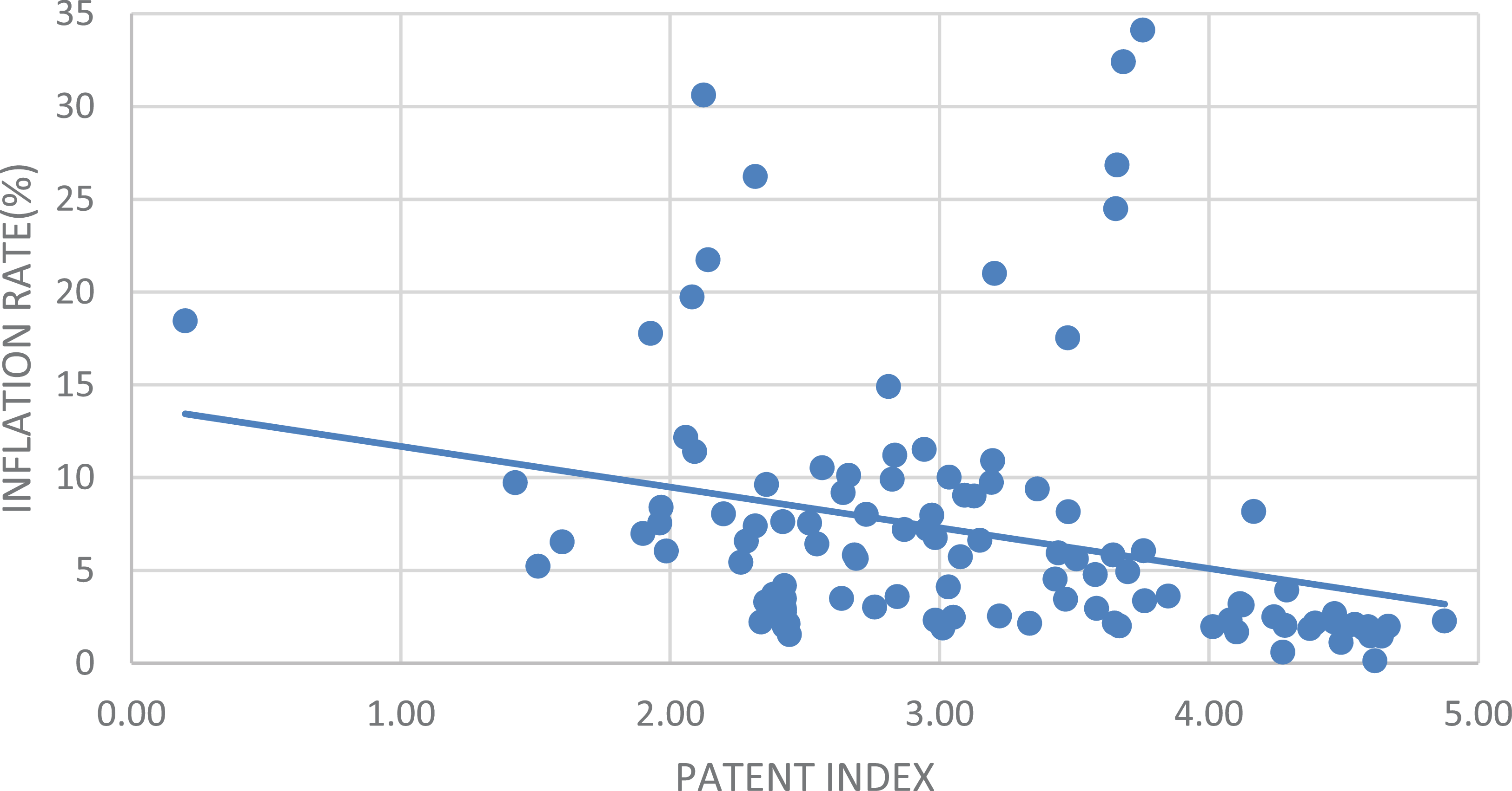
To this end, we construct an R&D-based growth model in which money demand arises from the cash-in-advance (CIA) constraint. The model is based on the standard variety-expansion model of Grossman and Helpman (Reference Grossman and Helpman1991, Ch.3) to analytically obtain the welfare-maximizing money growth rate. The main results are as follows: First, we analytically derive the welfare-maximizing growth rate of money. As mentioned previously, an increase in money growth has two opposing effects on welfare. On the one hand, an increase in money growth raises the government’s revenue, and this reduces income tax. A lower tax rate promotes R&D and economic growth, and thus raises welfare. On the other hand, higher money growth induces a higher nominal interest rate and reduces welfare. Welfare-maximizing money growth is determined to balance these opposing effects. Second, stronger patent protection reduces the welfare-maximizing money growth rate. The reason for this result is as follows. An increase in money growth raises the nominal interest rate, which reduces the labor supply under the CIA constraint. Stronger patent protection has a negative effect on the wage rate because it enables firms to raise the price of goods by reducing the production volume, which consequently reduces the demand for labor and wages. Hence, it strengthens the labor supply reducing effect of money growth. Owing to this effect, stronger patent protection reduces the growth-enhancing effect of money growth and lowers the welfare-maximizing money growth. This theoretical result is consistent with the observed tendency for the inflation rates to be relatively low in developed countries, where patent protection is stronger.Footnote 2 We can confirm that this theoretical result matches the cross–country data. Figure 1 is the actual relationship between the strength of patent protection and inflation rates. This shows that the inflation rate is negatively associated with the strength of patent protection.Footnote 3
Relationship between patent protection and inflation.
Note: We collect cross-country data on the strength of patent protection and inflation from Park (Reference Park2008) and the World Bank, respectively. The horizontal axis represents the index of patent protection. The index is a scale of 0–5, and a larger number indicates stronger patent protection. The vertical axis represents inflation rates (%). Park (Reference Park2008) consists of 122 countries’ data. The period for which the data of patent index for all the countries are available is from 1995 to 2015, and thus we use the average patent index and inflation rates in this period. Moreover, we exclude some countries for the following reasons. First, the WB dataset does not have data of inflation rates of Argentina, Somalia and Taiwan, and thus we exclude them. Second, Angola, Zaire, Bulgaria and Venezuela have extremely high inflation rates over 40% in this period, thus we exclude them. As a result, we use data from 115 countries. The solid line represents the fitted line. The coefficient of the line is $-2.19$
and the standard error is
$-2.19$
and the standard error is $0.69$
. Then the t-value is
$0.69$
. Then the t-value is $-3.17$
, and thus the coefficient is significantly negative.
$-3.17$
, and thus the coefficient is significantly negative.

Numerous studies have examined the effects of monetary policy – the growth rate of the money stock – in R&D-based growth models where the productivity growth rate is endogenous.Footnote 4 In an economy in which productivity growth is endogenous, stronger protection of intellectual property rights (IPR), including patents, has a significant impact on the economy in the following ways. First, stronger protection of IPR usually strengthens the power of monopolies and raises profits through invention, thus enhancing R&D activities. Conversely, as mentioned previously, the stronger power of the monopoly reduces the demand for factors of production and lowers the factor price, such as wages. Hence, IPR protection has an impact on the effect of money growth on growth and welfare. Chu et al. (Reference Chu, Lai and Liao2019), one of the seminal papers in the literature examine how the effects of money growth on growth and welfare depend on patent protection in a variety-expansion model. Conversely, using a quality ladder model, Huang, Yang, and Cheng (Reference Huang, Yang and Cheng2017) examined the growth and welfare effects of monetary and patent policies and compared the effects of the two policies. However, neither study considers a channel through which an increase in money growth reduces the income tax rate by loosening the government’s budget constraints. Without this channel, an increase in money growth would only have a negative effect on welfare in usual situations. Thus, in their models, setting the money growth rate so that the nominal interest rate is zero, the so-called ”the Friedman rule,” maximizes welfare.Footnote 5 The Friedman rule implies that the optimal inflation rate is negative as long as the real interest rate is positive, which appears to be inconsistent with many real-world situations in which moderate positive inflation is commonly observed. In contrast, the present paper highlights a positive role for inflation through seigniorage revenue used as a fiscal policy instrument. In particular, higher money growth can reduce distortionary income taxation and thereby promote innovation. As a result, the optimal inflation rate in this framework is more likely to be positive, which is consistent with many realistic situations. Moreover, the model allows us to examine how the optimal inflation rate depends on key structural parameters, including R&D productivity, as well as policy variables such as patent protection and R&D subsidies. This mechanism provides a novel perspective on the relationship between inflation and innovation-driven growth.
Several studies, such as Shaw et al. (Reference Shaw, Chang and Lai2006), Ho, Zheng, and Zhang (Reference Ho, Zeng and Zhang2007), and Chang et al. (Reference Chang, Tsai, Chang and Lee2015), examine welfare-maximizing money growth by considering the above channel and indicate the possibility that a positive nominal interest rate maximizes welfare. However, these models are growth models in which the engine of economic growth is only physical capital; thus, they cannot examine how the effects of money growth depend on policy variables such as patent protection and R&D subsidies. Hence, this study complements the aforementioned studies.
The remainder of this paper is organized as follows. Section 2 describes the model setup, and Section 3 characterizes the market equilibrium path. Section 4 derives the welfare-maximizing money growth rate and examines its dependence on the strength of patent protection. Moreover, it shows whether the Friedman rule, namely, a zero nominal interest rate maximizes welfare depends on the degree of the patent protection. Section 5 shows that a zero nominal interest rate maximizes welfare when seigniorage reduces a lump-sum tax rather than a distortionary tax. Section 6 concludes.
2. Model
To analytically examine the effects of money growth on economic growth and welfare, we incorporate the CIA constraint of consumption and endogenous labor supply into the standard R&D-based growth model of Grossman and Helpman (Reference Grossman and Helpman1991, Ch.3). Under the CIA constraint, people require money in advance to consume goods. The nominal interest rate is the cost of consumption and consequently, its rise reduces consumption, which is the benefit of labor supply. Higher money growth induces higher inflation and nominal interest rates, which reduce the benefit of labor supply and reduce labor supply, thus impeding economic growth. Conversely, money growth also increases government revenue and lowers taxes including corporate income tax, thereby enhancing economic growth. Through this mechanism, we examine how money growth affects economic growth and social welfare.
2.1 Households
There exists one representative household in the economy. The household supplies labor $\ell (t) (\!\in\![0, \bar {\ell }])$
elastically. The lifetime utility of the household is given by
$\ell (t) (\!\in\![0, \bar {\ell }])$
elastically. The lifetime utility of the household is given by
 \begin{eqnarray} U=\int _0^\infty e^{-\rho t} \left [ \ln c(t) + \gamma \ln \left ( \bar {\ell }-\ell (t) \right ) \right ] dt, \end{eqnarray}
where $\rho$
denotes the discount rate,
$\rho$
denotes the discount rate, $c(t)$
denotes the consumption of goods, and
$c(t)$
denotes the consumption of goods, and $\gamma$
represents the weight of the utility from leisure
$\gamma$
represents the weight of the utility from leisure $(\bar {\ell }-\ell (t))$
. We let
$(\bar {\ell }-\ell (t))$
. We let $\tau _w$
denote the labor income tax rate. The household budget constraint is
$\tau _w$
denote the labor income tax rate. The household budget constraint is
 \begin{eqnarray*} \dot {a}(t) &=& r(t) a(t) +(1-\tau _w) w(t) \ell (t) -c(t)- \pi (t) m(t)-T(t) - s(t), \\ \dot {m}(t) &=& s(t), \end{eqnarray*}
where $r(t)$
,
$r(t)$
, $w(t)$
,
$w(t)$
, $\pi (t)$
,
$\pi (t)$
, $a(t)$
,
$a(t)$
, $m(t)$
,
$m(t)$
, $T(t)$
, and
$T(t)$
, and $s(t)$
denote the real interest rate, real wage rate, inflation rate, asset holdings, real money holdings, lump-sum tax, and the increase in money holdings, respectively.
$s(t)$
denote the real interest rate, real wage rate, inflation rate, asset holdings, real money holdings, lump-sum tax, and the increase in money holdings, respectively.
The household must have money in advance to consume the good; that is, we assume a CIA constraint. Moreover, to consider a general situation, we assume that a fraction of consumption expenditure $\xi (\!\in\!(0,1])$
is subject to the following CIA constraint:
$\xi (\!\in\!(0,1])$
is subject to the following CIA constraint:
 \begin{eqnarray} \xi c(t) \le m(t). \end{eqnarray}
We let $\lambda (t)$
denote the costate variable for
$\lambda (t)$
denote the costate variable for $a(t)$
, as in Appendix A. The optimality condition for consumption is
$a(t)$
, as in Appendix A. The optimality condition for consumption is
 \begin{eqnarray} \frac {1}{c(t)} =\left [ 1+\xi i(t) \right ] \lambda (t), \end{eqnarray}
where $i(t)$
denotes the nominal interest rate and satisfies the Fisher equation,
$i(t)$
denotes the nominal interest rate and satisfies the Fisher equation, $i(t)=r(t)+\pi (t)$
. The optimality condition for labor supply is
$i(t)=r(t)+\pi (t)$
. The optimality condition for labor supply is
 \begin{eqnarray} \gamma \frac {1}{\bar {\ell }-\ell (t)}=\frac {(1-\tau _w)w(t)}{\left [1+ \xi i(t) \right ] c(t)}. \end{eqnarray}
Additionally, we obtain
 \begin{eqnarray} \frac {\dot {\lambda }(t)}{\lambda (t)} =\rho -r(t). \end{eqnarray}
2.2 Firms
The consumption good can be produced by utilizing intermediate goods. Following Benassy (Reference Benassy1998), we assume the production function of the good as follows.
 \begin{eqnarray} Y(t) =n(t)^{\nu -\left (\frac {1}{\alpha }-1\right )} \left [ \int _0^{n(t)} x(i, t)^\alpha di \right ]^\frac {1}{\alpha }, \quad 0\lt \alpha \lt 1, \end{eqnarray}
where $x(i,t)$
denotes the volume of intermediate good
$x(i,t)$
denotes the volume of intermediate good $i$
for
$i$
for $i \in [0,n(t)]$
,
$i \in [0,n(t)]$
, $\frac {1}{1-\alpha } (\gt 1)$
represents the elasticity of substitution among the intermediate goods, and
$\frac {1}{1-\alpha } (\gt 1)$
represents the elasticity of substitution among the intermediate goods, and $\nu (\gt 0)$
represents the degree of the contribution of variety
$\nu (\gt 0)$
represents the degree of the contribution of variety $n$
to productivity. The higher the
$n$
to productivity. The higher the $\nu$
, the greater the contribution of variety to productivity. Hereafter, we refer to this parameter as the contribution of R&D to productivity.Footnote
6
By using this specification of production function, we can disentangle the elasticity of substitution and the contribution of R&D to productivity. We let
$\nu$
, the greater the contribution of variety to productivity. Hereafter, we refer to this parameter as the contribution of R&D to productivity.Footnote
6
By using this specification of production function, we can disentangle the elasticity of substitution and the contribution of R&D to productivity. We let $P(t)$
denote the price of the good. We assume that perfect competition prevails in the good market. By solving the cost-minimization problem for firms, given the production volume of good
$P(t)$
denote the price of the good. We assume that perfect competition prevails in the good market. By solving the cost-minimization problem for firms, given the production volume of good $Y(t)$
, we obtain the demand for the intermediate good
$Y(t)$
, we obtain the demand for the intermediate good $i$
as follows:
$i$
as follows:
 \begin{equation} x(i, t) = \left ( \frac {P(i, t)}{P(t)} \right )^{-\frac {1}{1-\alpha }} Y(t) n(t)^{\frac {\alpha }{1-\alpha }\nu -1}. \end{equation}
where $P(i,t)$
denotes the price of intermediate good
$P(i,t)$
denotes the price of intermediate good $i$
. Moreover, we obtain the unit cost, that is, the minimized cost of producing one unit of the good as
$i$
. Moreover, we obtain the unit cost, that is, the minimized cost of producing one unit of the good as $n(t)^{-(\nu - (\frac {1}{\alpha }-1 ))} [ \int _0^{n(t)} P(i, t)^{-\frac {\alpha }{1-\alpha }} di ]^{-\frac {1-\alpha }{\alpha }}.$
Perfect competition prevails, and thus the price of the final good equals this unit cost:
$n(t)^{-(\nu - (\frac {1}{\alpha }-1 ))} [ \int _0^{n(t)} P(i, t)^{-\frac {\alpha }{1-\alpha }} di ]^{-\frac {1-\alpha }{\alpha }}.$
Perfect competition prevails, and thus the price of the final good equals this unit cost:
 \begin{eqnarray} P(t)=n(t)^{-\left(\nu -\left (\frac {1}{\alpha }-1\right )\right)} \left [ \int _0^{n(t)} P(i, t)^{-\frac {\alpha }{1-\alpha }} di \right ]^{-\frac {1-\alpha }{\alpha }}. \end{eqnarray}
2.2.1 Intermediate goods
One unit of each intermediate good is produced using one unit of labor. Each intermediate good is supplied monopolistically by a firm with a patent.
We must consider how governments protect patents. Generally, governments control the degree of patent protection through patent length and patent breadth. However, for simplicity, we assume that patent length is fixed and infinite and governments control the degree of patent protection using only patent breadth.Footnote
7
Following Goh and Olivier (Reference Goh and Olivier2002), we assume that when the patent breadth is broader, it is more difficult to produce imitative goods. We let $W(t)$
denote the nominal wage rate. We specify the unit cost of producing imitative goods as
$W(t)$
denote the nominal wage rate. We specify the unit cost of producing imitative goods as $\beta W(t) \ (\beta \in (1, 1/\alpha ])$
; where strengthening patent protection increases
$\beta W(t) \ (\beta \in (1, 1/\alpha ])$
; where strengthening patent protection increases $\beta$
. A firm that produces each intermediate good charges its price such that producers of imitative goods cannot earn a positive profit as follows:
$\beta$
. A firm that produces each intermediate good charges its price such that producers of imitative goods cannot earn a positive profit as follows:
 \begin{eqnarray} \displaystyle P(i,t)=\beta W(t). \end{eqnarray}
When $\beta$
obtains the highest value
$\beta$
obtains the highest value $1/\alpha$
, that is, when the patent breadth is the broadest, the price is equal to the monopoly price.
$1/\alpha$
, that is, when the patent breadth is the broadest, the price is equal to the monopoly price.
By substituting (9) into (8), we obtain the relationship between price of final good $P(t)$
and nominal wage
$P(t)$
and nominal wage $W(t)$
as
$W(t)$
as $P(t)=n(t)^{-\nu } \beta W(t)$
. From this, we obtain the real wage rate
$P(t)=n(t)^{-\nu } \beta W(t)$
. From this, we obtain the real wage rate $w(t) \equiv W(t)/P(t)$
as follows:Footnote
8
$w(t) \equiv W(t)/P(t)$
as follows:Footnote
8
 \begin{eqnarray} w(t)=\frac {1}{\beta } n(t)^\nu . \end{eqnarray}
Because intermediate goods firms charge the same price, they produce the same volume. Letting $x(t)$
denote the symmetric production volume, from (6), we obtain
$x(t)$
denote the symmetric production volume, from (6), we obtain
 \begin{equation} x(t) = n(t)^{-(\nu +1)} Y(t). \end{equation}
The real profit of the intermediate goods firm $i$
is
$i$
is $ \left ( p(i,t) -w(t) \right ) x(i, t),$
where
$ \left ( p(i,t) -w(t) \right ) x(i, t),$
where $p(i, t) \equiv P(i, t)/P(t)$
is the real price of intermediate good
$p(i, t) \equiv P(i, t)/P(t)$
is the real price of intermediate good $i$
. Therefore, we obtain the real profit of the intermediate goods firm
$i$
. Therefore, we obtain the real profit of the intermediate goods firm $\Pi (t)$
as follows:
$\Pi (t)$
as follows:
 \begin{equation} \Pi (t) =(p(i,t)-w(t))x(t) =(\beta -1) \frac {Y(t)}{\beta n(t)}. \end{equation}
2.2.2 R&D
Finally, we consider the behavior of R&D firms. We assume that R&D firms can invent a new intermediate good by devoting $\bar {a}(t)$
units of labor. Letting
$\bar {a}(t)$
units of labor. Letting $\ell _R(t)$
denote the labor devoted to R&D activities, then, we can express the R&D technology as
$\ell _R(t)$
denote the labor devoted to R&D activities, then, we can express the R&D technology as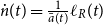 $\dot {n}(t) = \frac {1}{\bar {a}(t)} \ell _R(t)$
. We assume the presence of knowledge spillovers from the past R&D activities and thus assume that an increase in
$\dot {n}(t) = \frac {1}{\bar {a}(t)} \ell _R(t)$
. We assume the presence of knowledge spillovers from the past R&D activities and thus assume that an increase in $n(t)$
reduces the R&D cost
$n(t)$
reduces the R&D cost $\bar {a}(t)$
. Moreover, we assume
$\bar {a}(t)$
. Moreover, we assume $\bar {a}(t) = a/n(t)$
, as in the first-generation endogenous growth models such as Romer (Reference Romer1990). Thus, the R&D technology becomes
$\bar {a}(t) = a/n(t)$
, as in the first-generation endogenous growth models such as Romer (Reference Romer1990). Thus, the R&D technology becomes
 \begin{eqnarray} \dot {n}(t) = \frac {n(t)}{a} \ell _R(t). \end{eqnarray}
We let $v(t)$
denote the real stock value of the intermediate goods. Then, the profit of an R&D firm is
$v(t)$
denote the real stock value of the intermediate goods. Then, the profit of an R&D firm is $v(t) dn - w(t) (a/n(t)) dn$
=
$v(t) dn - w(t) (a/n(t)) dn$
= $[v(t) -w(t) (a/n(t))] dn$
. The R&D equilibrium condition is given by
$[v(t) -w(t) (a/n(t))] dn$
. The R&D equilibrium condition is given by
 \begin{eqnarray} v(t) n(t) =w(t) a. \end{eqnarray}
The real stock value $v(t)$
must satisfy the no-arbitrage condition, as follows:
$v(t)$
must satisfy the no-arbitrage condition, as follows:
 \begin{eqnarray} r(t) = \frac {(1-\tau _\Pi )\Pi (t)}{v(t)} +\frac {\dot {v}(t)}{v(t)}, \end{eqnarray}
where $\tau _\Pi$
denotes the corporate income tax rate.
$\tau _\Pi$
denotes the corporate income tax rate.
2.3 Money supply
In this study, we consider the case in which the growth rate of the nominal money stock $M(t)$
is a constant
$M(t)$
is a constant $\mu$
; that is,
$\mu$
; that is, $\dot {M}{(t)}/M(t)=\mu$
. As Appendix B shows, by using the Fisher equation, we derive the nominal interest rate as follows:
$\dot {M}{(t)}/M(t)=\mu$
. As Appendix B shows, by using the Fisher equation, we derive the nominal interest rate as follows:
 \begin{eqnarray} i(t)=\rho +\mu . \end{eqnarray}
2.4 Government
In fact, governments can obtain revenue by increasing the inflation rate; that is, they earn revenue by issuing new money. In this study, we consider a situation where the government can reduce distortionary tax rates by issuing new money and generating revenue. Specifically, we assume that governments satisfy the bala nced budget constraint at each time point. The government hires $\ell _G$
units of labor to supply public services at each point in time. The government must satisfy the following budget constraint:
$\ell _G$
units of labor to supply public services at each point in time. The government must satisfy the following budget constraint: $\frac {\dot {M}(t)}{P(t)}+\tau _\Pi \Pi (t) n(t) + \tau _w w(t) \ell (t) +T(t)= w(t) \ell _G$
. The CIA constraint is binding; that is,
$\frac {\dot {M}(t)}{P(t)}+\tau _\Pi \Pi (t) n(t) + \tau _w w(t) \ell (t) +T(t)= w(t) \ell _G$
. The CIA constraint is binding; that is, $m(t)=\xi c(t)$
. Therefore, by rewriting this, we obtain
$m(t)=\xi c(t)$
. Therefore, by rewriting this, we obtain
 \begin{eqnarray} \mu \xi c(t)+\tau _\Pi \Pi (t) n(t) + \tau _w w(t) \ell (t) +\frac {T(t)}{c(t)}= w(t) \ell _G. \end{eqnarray}
The government can choose the tax rates for corporate and labor income considering the budget constraint above.
3. Market equilibrium
In this section, we derive the market equilibrium path.
In this economy, due to knowledge spillovers, the number of varieties of goods grows at a positive constant rate. As mentioned above, $n(t)^\nu$
represents productivity in this economy. As will be shown later, there exists a balanced growth path along which productivity
$n(t)^\nu$
represents productivity in this economy. As will be shown later, there exists a balanced growth path along which productivity $n(t)^\nu$
and consumption
$n(t)^\nu$
and consumption $c(t)$
grow at the same rate.Footnote
9
$c(t)$
grow at the same rate.Footnote
9
On the balanced growth path, the ratio of consumption to $n(t)^\nu$
is constant, and thus, we define
$n(t)^\nu$
is constant, and thus, we define $z(t) \equiv \frac {c(t)}{n(t)^\nu }$
:
$z(t) \equiv \frac {c(t)}{n(t)^\nu }$
: $Y(t)=n(t)^\nu [n(t)x(t)]$
where
$Y(t)=n(t)^\nu [n(t)x(t)]$
where $n(t)x(t)$
represents the volume of labor input devoted to production and
$n(t)x(t)$
represents the volume of labor input devoted to production and $n(t)^\nu$
represents the total factor productivity (TFP) of the economy. Thus,
$n(t)^\nu$
represents the total factor productivity (TFP) of the economy. Thus, $z(t)$
denotes the consumption-to-productivity ratio. We characterize the market equilibrium path using
$z(t)$
denotes the consumption-to-productivity ratio. We characterize the market equilibrium path using $z(t)$
.
$z(t)$
.
First, we derive the equilibrium labor supply: Substituting (10) and (16) into (4) and rewriting it yields
 \begin{eqnarray} \ell (t) =\bar {\ell } - \gamma \frac {1+ \xi (\rho +\mu )}{1-\tau _w} \beta z(t), \end{eqnarray}
which is determined by $z(t)$
. Subsequently, the labor market equilibrium condition is
$z(t)$
. Subsequently, the labor market equilibrium condition is $\ell (t) = \ell _G + \frac {a}{n(t)} \dot {n}(t) + n(t) x(t)$
. From (11),
$\ell (t) = \ell _G + \frac {a}{n(t)} \dot {n}(t) + n(t) x(t)$
. From (11), $n(t)x(t)= \frac {c(t)}{n(t)^\nu } =z(t)$
. Using these expressions, we obtain the growth rate of
$n(t)x(t)= \frac {c(t)}{n(t)^\nu } =z(t)$
. Using these expressions, we obtain the growth rate of $n(t)$
as follows:
$n(t)$
as follows:
 \begin{eqnarray} \displaystyle \frac { \dot {n}(t) }{n(t)}= \frac {1}{a} \left [ \ell (t) - \ell _G -z(t) \right ], \end{eqnarray}
which is determined by $z(t)$
. From (3), (5), and (16), we obtain the growth rate of
$z(t)$
. From (3), (5), and (16), we obtain the growth rate of $c(t)$
as follows:
$c(t)$
as follows:
 \begin{eqnarray} \frac {\dot {c}{(t)}}{c(t)} =r(t)-\rho . \end{eqnarray}
We derive the real interest rate to determine the growth rate of $c(t)$
. From (10), (12), (14), and (15), we obtain
$c(t)$
. From (10), (12), (14), and (15), we obtain
 \begin{eqnarray} r(t) = \frac {(1-\tau _\Pi ) \Pi (t)n(t)}{a w(t)} +\frac {\dot {w}(t)}{w(t)} - \frac {\dot {n}(t)}{n(t)} = \frac {(1-\tau _\Pi )(\beta -1)}{a}z(t) +\nu \frac {\dot {n}(t)}{n(t)} - \frac {\dot {n}(t)}{n(t)}. \end{eqnarray}
Finally, we derive the differential equation for only $z(t)$
. Considering the logarithm of both sides of
$z(t)$
. Considering the logarithm of both sides of $z(t) \equiv \frac {c(t)}{n(t)^\nu }$
, we obtain
$z(t) \equiv \frac {c(t)}{n(t)^\nu }$
, we obtain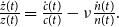 $ \frac {\dot {z}(t)}{z(t)} = \frac {\dot {c}(t)}{c(t)} - \nu \frac {\dot {n}(t)}{n(t)}.$
Substituting (3), (19), (20), and (21) into the RHS of this equation yields the growth rate of
$ \frac {\dot {z}(t)}{z(t)} = \frac {\dot {c}(t)}{c(t)} - \nu \frac {\dot {n}(t)}{n(t)}.$
Substituting (3), (19), (20), and (21) into the RHS of this equation yields the growth rate of $z(t)$
as follows:
$z(t)$
as follows:
 \begin{eqnarray} \frac {\dot {z}(t)}{z(t)} &=& \frac {(1-\tau _\Pi )(\beta -1)}{a}z(t) - \frac {\dot {n}(t)}{n(t)} -\rho \nonumber \\ &=& \frac {(1-\tau _\Pi )(\beta -1)}{a}z(t) - \frac {1}{a} \left [ \ell (t) - \ell _G -z(t) \right ]-\rho , \end{eqnarray}
where $\ell (t)$
is expressed by (18).
$\ell (t)$
is expressed by (18).
We assume that the government is unable to employ lump-sum taxation and therefore must rely on distortionary taxes to finance public expenditure. In particular, we consider a public finance regime in which the labor income tax rate is constant and the corporate income tax rate is endogenously determined to satisfy the budget constraint (17). By substituting $T(t)=0$
and (10) into (17) and dividing both sides by
$T(t)=0$
and (10) into (17) and dividing both sides by $c(t)$
, we obtain
$c(t)$
, we obtain $ \mu \xi +\tau _\Pi \frac {\Pi (t) n(t)}{c(t)} + \tau _w \frac {n(t)^\nu \ell (t)}{\beta c(t)} = \frac {n(t)^\nu \ell _G}{ \beta c(t)}.$
Using
$ \mu \xi +\tau _\Pi \frac {\Pi (t) n(t)}{c(t)} + \tau _w \frac {n(t)^\nu \ell (t)}{\beta c(t)} = \frac {n(t)^\nu \ell _G}{ \beta c(t)}.$
Using $z(t)$
, we can rewrite the equation above as follows:
$z(t)$
, we can rewrite the equation above as follows: $ \mu \xi + \tau _\Pi ( 1-\frac {1}{\beta } ) + \tau _w \frac {\ell (t)}{\beta z(t)} = \frac {\ell _G}{\beta z(t)}.$
Subsequently, the corporate income tax rate is endogenously determined asFootnote
10
$ \mu \xi + \tau _\Pi ( 1-\frac {1}{\beta } ) + \tau _w \frac {\ell (t)}{\beta z(t)} = \frac {\ell _G}{\beta z(t)}.$
Subsequently, the corporate income tax rate is endogenously determined asFootnote
10
 \begin{eqnarray} \tau _\Pi (t) \left ( 1-\frac {1}{\beta } \right ) = \frac {\ell _G-\tau _w \ell (t)}{\beta z(t)}-\mu \xi . \end{eqnarray}
By substituting (18) and (23) into (22), we obtain the differential equation for $z(t)$
as follows:
$z(t)$
as follows:
 \begin{eqnarray*} \frac {\dot {z}(t)}{z(t)} &=& \left \{ \mu \xi +1+\gamma [1+\xi (\rho +\mu )] \right \}\frac {\beta }{a}z(t) - \left [(1-\tau _w) \frac {\bar {\ell }}{a} +\rho \right ]. \end{eqnarray*}
A unique interior steady state exists. Letting $z^\ast$
denote the steady-state level of
$z^\ast$
denote the steady-state level of $z$
, we obtain
$z$
, we obtain
 \begin{eqnarray} z^\ast = \frac {(1-\tau _w) \bar {\ell } +\rho a}{\beta \left \{ \mu \xi +1+\gamma [1+\xi (\rho +\mu )] \right \}}. \end{eqnarray}
The unique interior steady state, $z^\ast$
is unstable. If
$z^\ast$
is unstable. If $z(0)$
is not equal to
$z(0)$
is not equal to $z^\ast$
,
$z^\ast$
, $z(t)$
diverges to a negative or positive infinity. Thus,
$z(t)$
diverges to a negative or positive infinity. Thus, $z(t)$
is equal to
$z(t)$
is equal to $z^\ast$
from the initial point in time.
$z^\ast$
from the initial point in time. $z(t)$
is constant, and from (18)
$z(t)$
is constant, and from (18) $\ell (t)$
is constant. Substituting these into (19), the growth rate of
$\ell (t)$
is constant. Substituting these into (19), the growth rate of $n(t)$
is determined as follows:
$n(t)$
is determined as follows:
 \begin{eqnarray} g_n^\ast \equiv \frac {\dot {n}(t)}{n(t)} = \frac {1}{a} \left \{ \bar {\ell } - \ell _G - \left [ 1+\gamma \beta \frac {1+\xi (\rho +\mu )}{1-\tau _w} \right ] z^\ast \right \}. \end{eqnarray}
All the other macroeconomic variables are constant or growing at constant rates. Thus, the balanced equilibrium path is obtained. Hereafter, we limit our analysis to cases in which the growth rate is nonnegative. Differentiating (25) with respect to $\mu$
yields
$\mu$
yields
 \begin{eqnarray} \displaystyle \frac {\partial g_n^\ast }{\partial \mu } &=& \xi \gamma \beta \frac {z^\ast }{a} \left \{ -\frac {1}{1-\tau _w} + \left [ \frac { 1+\xi (\rho +\mu )}{1-\tau _w} + \frac {1}{\gamma \beta } \right ] \frac {1+\gamma }{\gamma [1+\xi (\rho +\mu )] +1+\xi \mu } \right \} \nonumber \\ &=& \xi \gamma \beta \frac {z^\ast }{a} \frac {\frac {1}{1-\tau _w} \xi \rho +\frac {1+\gamma }{\gamma \beta } }{\gamma [1+\xi (\rho +\mu )] +1+\xi \mu } \gt 0. \end{eqnarray}
Therefore, the growth rate is an increasing function of $\mu$
, and we can summarize the results as follows:
$\mu$
, and we can summarize the results as follows:
Proposition 1. Under a regime in which an increase in seigniorage, that is, revenue from issuing new money, reduces corporate income tax, an increase in money growth enhances economic growth.
The reasons for this result are as follows. As shown in (25), an increase in the nominal money stock growth rate has two opposing effects: On the one hand, it raises the inflation rate and nominal interest rates. As shown in (18), an increase in the nominal interest rate reduces labor supply and consequently lowers the growth rate. On the other hand, it increases seigniorage, which lowers the corporate income tax rate, and thus promotes R&D and economic growth. As shown in the results, in this model, the latter’s positive effect overwhelms the former’s negative effect.Footnote 11
To understand the direct effect of an increase in money growth, we consider the case in which an increase in money growth – an increase in seigniorage – does not reduce the corporate income tax rate. In other words, we consider the case in which the government is able to employ lump-sum transfer, and money growth does not lower the distortionary tax rate. In this lump-sum transfer regime, an increase in money growth has only the aforementioned negative effect on economic growth. As shown in Appendix C, stronger patent protection strengthens this negative effect. We summarize the results in the following proposition:
Proposition 2. In a regime in which seigniorage is distributed in lump-sum transfers and corporate income tax is constant, an increase in money growth impedes economic growth. Moreover, stronger patent protection strengthens the negative growth effect.
The intuition for the second result is as follows. An increase in money growth raises the nominal interest rate, which reduces labor supply. Stronger patent protection has a negative effect on the wage rate, as shown in (10). This is because it enables firms to raise the price of goods by reducing the production volume, which consequently reduces the demand for labor and wages. Hence, it strengthens the labor supply reducing effect of money growth.
4. Welfare analysis of money growth
4.1 Welfare-maximizing money growth rate
Subsequently, we examine how an increase in the growth rate of the nominal money stock affects welfare.
First, we derive welfare as a function of the growth rate of nominal money stock $\mu$
. The economy is on a balanced growth path, where
$\mu$
. The economy is on a balanced growth path, where $z(t)(\equiv c(t)/n(t)^\nu )$
is equal to
$z(t)(\equiv c(t)/n(t)^\nu )$
is equal to $z^\ast$
, as previously shown. Therefore, consumption can be rewritten as
$z^\ast$
, as previously shown. Therefore, consumption can be rewritten as $c(t)=z^\ast n(t)^\nu$
. Moreover, from (18), leisure is constant over time and is determined by
$c(t)=z^\ast n(t)^\nu$
. Moreover, from (18), leisure is constant over time and is determined by $z^\ast$
. Substituting these into the utility function, we obtain
$z^\ast$
. Substituting these into the utility function, we obtain
 \begin{eqnarray} U &=&\int _0^\infty e^{-\rho t} \left \{ \ln c(t) + \gamma \ln \left [ \bar {\ell } -\ell (t) \right ] \right \} dt \nonumber \\ &=& \int _0^\infty e^{-\rho t} \left \{ \ln z^\ast + \nu \left [ g_n^\ast t +\ln n(0) \right ] + \gamma \ln \left ( \bar {\ell } -\ell ^\ast \right ) \right \} dt \nonumber \\ &=& \frac {1}{\rho } \left [ \ln z^\ast +\gamma \ln (\bar {\ell }-\ell ^\ast ) + \nu \frac {g_n^\ast }{\rho } + \nu \ln n(0) \right ]. \end{eqnarray}
In order to derive the welfare-maximizing money growth rate, we differentiate (27) with respect to $\mu$
. The derivative of
$\mu$
. The derivative of $U$
is given by:
$U$
is given by:
 \begin{align} \displaystyle \frac {\partial U}{\partial \mu } = \frac {1}{\rho } \Bigl [ \underbrace { \frac {1}{z^\ast } \frac {\partial z^\ast }{\partial \mu }} _{\stackrel {\mbox{consumption-reducing effect}}{\mbox{(-)}}} \quad + \quad \underbrace { \gamma \frac {1}{\bar {\ell }-\ell ^\ast } \frac {\partial (\bar {\ell }-\ell ^\ast )}{\partial \mu }} _{\stackrel {\mbox{leisure-saving effect}}{\mbox{(+)}}} \quad + \quad \underbrace {\frac {1}{\rho } \nu \frac {\partial g_n^\ast }{\partial \mu }} _{\stackrel {\mbox{tax-reducing effect}}{\mbox{(+)}}} \Bigr ]. \end{align}
An increase in money growth affects welfare though the following channels. First, an increase in money growth raises the inflation rate and the nominal interest rate. Because the nominal interest is the relative cost of consumption to leisure under the CIA constraint, this consequently reduces consumption and increases leisure. The first effect reduces welfare and the second raises welfare. We refer to the first and second effects as the consumption-reducing effect and leisure-saving effect respectively. They are indicated by the first and second terms on the right-hand side (RHS) of (28). Finally, an increase in money growth raises revenue from issuing new money. This allows a reduction of corporate income tax through the balanced budget constraint and enhances innovation and thus raises welfare. We refer to this effect as the tax-reducing effect. This positive welfare effect is indicated by the third term on the RHS of (28).
The former two effects relate to the static allocation between consumption and leisure. We refer to the sum of these two effects as the static allocation effect. Using (18), we can rewrite the part related to static allocation in the utility as follows:
 \begin{eqnarray} U &=& \frac {1}{\rho } \left [ (1+\gamma ) \ln z^\ast +\gamma \ln \left [ 1+\xi (\rho +\mu ) \right ] +\nu \frac {g_n^\ast }{\rho } + \nu \ln n(0) \right ]. \end{eqnarray}
Differentiating this again, we decompose the welfare effect into the following two parts:
 \begin{eqnarray} \displaystyle \frac {\partial U}{\partial \mu } = \frac {1}{\rho } \Bigl [ \underbrace { (1+\gamma ) \frac {1}{z^\ast } \frac {\partial z^\ast }{\partial \mu } + \gamma \frac {\xi }{ 1+\xi (\rho +\mu )} } _{\stackrel {\mbox{static-allocation effect}}{\mbox{(-)}}} \quad + \quad \underbrace {\frac {1}{\rho } \nu \frac {\partial g_n^\ast }{\partial \mu }} _{\stackrel {\mbox{tax-reducing effect}}{\mbox{(+)}}} \Bigr ]. \end{eqnarray}
From (24), we obtain
 \begin{eqnarray} \displaystyle \frac {1}{z^\ast } \frac {\partial z^\ast }{\partial \mu } = -\frac {(1+\gamma )\xi }{\gamma [1+\xi (\rho +\mu )] +1+\xi \mu }\lt 0. \end{eqnarray}
Rewriting the static allocation effect, we obtain
 \begin{align} \displaystyle (1+\gamma ) \frac {1}{z^\ast } \frac {\partial z^\ast }{\partial \mu } + \gamma \frac {\xi }{ 1+\xi (\rho +\mu )} = -\frac {(1+\gamma )\xi }{\gamma [1+\xi (\rho +\mu )] +1+\xi \mu } \left [ 1+ \frac {\gamma }{1+\gamma } \frac {\xi \rho }{ 1+\xi (\rho +\mu )} \right ] \lt 0. \end{align}
Thus, the static allocation effect is negative. This is because an increase in money growth increases nominal interest rates and distort the allocation between consumption and leisure activities. This static allocation effect is the marginal cost (MC) of raising money growth, while the tax-reducing effect is the marginal benefit (MB) of raising money growth. Thus, the welfare-maximizing growth rate of money is determined so that MB is equal to MC.
As shown in Appendix D, the welfare-maximizing growth rate of money is uniquely determined, and that this level is negatively correlated with the patent protection strength. We summarize the results in the following proposition:
Proposition 3. Under a regime in which an increase in seigniorage – revenue from issuing new money – reduces corporate income tax, there is a welfare-maximizing growth rate for nominal money stock.
ting $\mu ^\ast$
denote the money growth rate, we can analytically derive the following:
$\mu ^\ast$
denote the money growth rate, we can analytically derive the following:
 \begin{eqnarray} \displaystyle \mu ^\ast = \frac {\rho }{2(1+\gamma )} \left [ \frac {\Omega }{\xi \rho } + 1-\gamma +\sqrt {\left (\frac {\Omega }{\xi \rho } +1-\gamma \right )^2 +4 \gamma } \right ] - \left (\frac {1}{\xi }+\rho \right ), \end{eqnarray}
where
 \begin{eqnarray} \displaystyle \Omega \equiv \frac {1}{\rho } \nu \left ( \frac {\bar {\ell }}{a} +\frac {\rho }{1-\tau _w} \right ) \left (\frac {1-\tau _w}{\beta }+\frac {\gamma }{1+\gamma }\xi \rho \right ). \end{eqnarray}
From (
33
) and (
34
), stronger patent protection (higher $\beta$
) reduces the welfare-maximizing money growth rate.
$\beta$
) reduces the welfare-maximizing money growth rate.
The reason for this result is as follows. First, in a regime in which the corporate income tax rate is constant, that is, where an increase in money growth does not lower the corporate income tax rate, as shown in Appendix C, stronger patent protection strengthens the negative effect of an increase in money growth on the output growth rate. The intuition is as mentioned below Proposition2: A rise in money growth raises the nominal interest rate, which reduces labor supply. Here, stronger patent protection induces a lower wage rate and strengthens the labor-supply-reducing effect of money growth. Owing to this effect, under the tax-reducing regime, stronger patent protection reduces the total positive growth effect of a rise in money growth and subsequently reduces the MB of a rise in money growth. Therefore, stronger patent protection reduces the welfare-maximizing money growth rate.
As we can see in Figure 1 in the introduction, the cross-country data show that the relationship between patent protection and inflation rates is negative. Therefore, the theoretical results of this study are consistent with actual tendencies.
4.2 Optimal monetary policy and patent protection
4.2.1 Optimal nominal interest rate
Finally, we examine whether the Friedman rule is optimal or not in this model. The Friedman rule is to set money growth rate such that the nominal interest rate equals zero, that is, $i(t)=0$
. In this case, the money growth rate is given by
$i(t)=0$
. In this case, the money growth rate is given by $\mu =-\rho$
. As is well known, the Friedman rule is likely to be optimal in the case where money growth is not used to reduce income taxes.Footnote
12
However, in the case where money growth can reduce the income tax rate such as the present setting, the Friedman rule tends to be suboptimal, as discussed by Phelps (Reference Phelps1973). At the end of this section, we examine how whether the Friedman rule (
$\mu =-\rho$
. As is well known, the Friedman rule is likely to be optimal in the case where money growth is not used to reduce income taxes.Footnote
12
However, in the case where money growth can reduce the income tax rate such as the present setting, the Friedman rule tends to be suboptimal, as discussed by Phelps (Reference Phelps1973). At the end of this section, we examine how whether the Friedman rule ( $i=0$
) is optimal or not depends on patent protection. As shown in Appendix E, we obtained the following results:
$i=0$
) is optimal or not depends on patent protection. As shown in Appendix E, we obtained the following results:
Proposition 4.
Suppose that the nominal interest rate is subject to the zero lower bound. We let $\bar {\beta }$
denote the patent breadth that satisfies
$\bar {\beta }$
denote the patent breadth that satisfies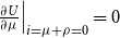 $\frac {\partial U}{\partial \mu }\Big |_{i=\mu +\rho =0}=0$
.
$\frac {\partial U}{\partial \mu }\Big |_{i=\mu +\rho =0}=0$
. $\bar {\beta }$
is given by
$\bar {\beta }$
is given by
 \begin{eqnarray*} \displaystyle \bar {\beta } \equiv \left [ \frac {(1+\gamma ) -(1-\gamma )\xi \rho + \frac {\gamma }{1+\gamma } \xi ^2 \rho ^2}{\frac {1}{\rho } \nu \left ( \frac {\bar {\ell }}{a} +\frac {\rho }{1-\tau _w} \right ) } - \frac {\gamma }{1+\gamma }\xi \rho \right ]^{-1}. \end{eqnarray*}
Whether the welfare-maximizing nominal interest rates $i^\ast$
is positive or zero depends on the strength of patent protection
$i^\ast$
is positive or zero depends on the strength of patent protection $\beta$
as follows:
$\beta$
as follows:
If (i) $\displaystyle \bar {\beta } \le 1$
,
$\displaystyle \bar {\beta } \le 1$
, $i^\ast =0$
for all
$i^\ast =0$
for all $\beta \in (1, \frac {1}{\alpha }]$
.
$\beta \in (1, \frac {1}{\alpha }]$
.
If (ii) $\displaystyle 1\lt \bar {\beta } \le \frac {1}{\alpha }$
, whether the welfare-maximizing nominal interest rate is positive or zero depends on the patent breadth as follows.
$\displaystyle 1\lt \bar {\beta } \le \frac {1}{\alpha }$
, whether the welfare-maximizing nominal interest rate is positive or zero depends on the patent breadth as follows.
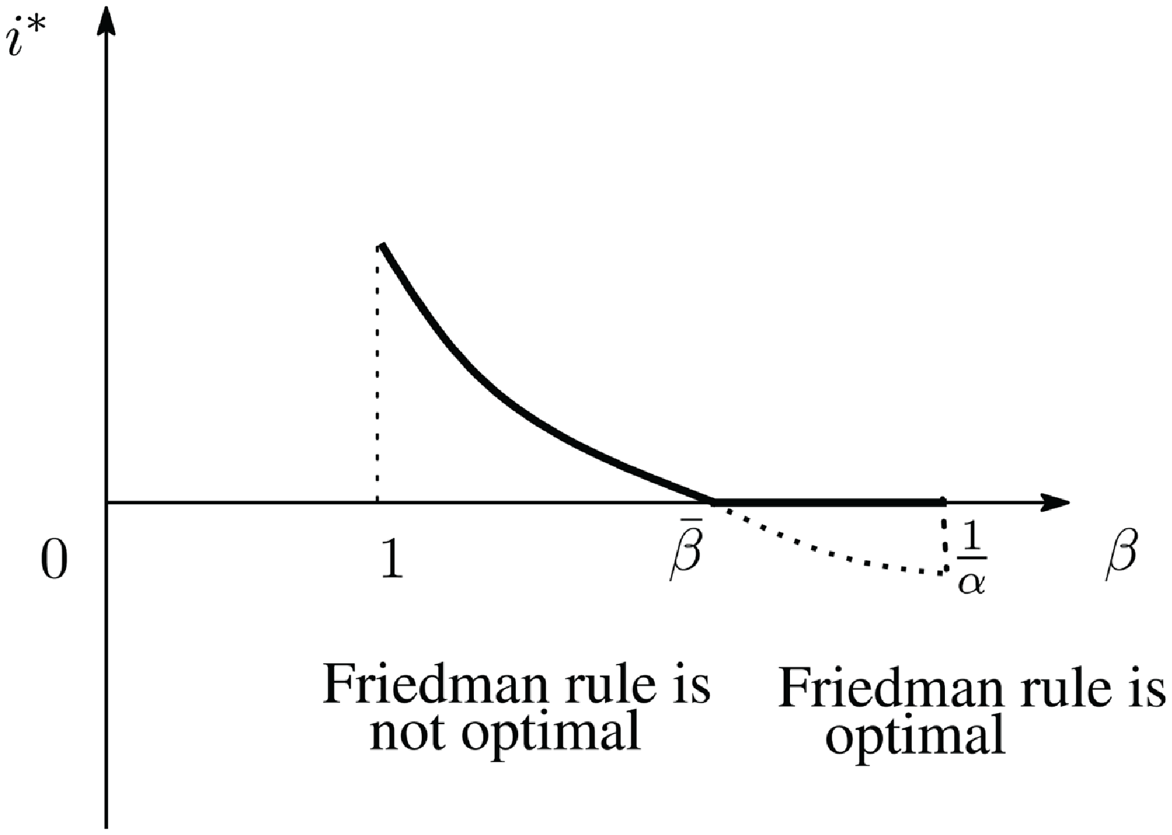
 \begin{align} i^\ast \begin{cases} \gt 0 \quad & \text{if} \ \ 1\lt \beta \lt \bar {\beta }, \\ =0 & \text{if} \ \ \bar {\beta } \le \beta \le \frac {1}{\alpha }, \end{cases} \end{align}
as depicted in Figure 2.
If (iii) $\displaystyle \frac {1}{\alpha }\lt \bar {\beta }$
,
$\displaystyle \frac {1}{\alpha }\lt \bar {\beta }$
, $i^\ast \gt 0$
for all
$i^\ast \gt 0$
for all $\beta \in (1, \frac {1}{\alpha }]$
.
$\beta \in (1, \frac {1}{\alpha }]$
.
The welfare-maximizing interest rate $i^\ast$
in case (ii).
$i^\ast$
in case (ii).
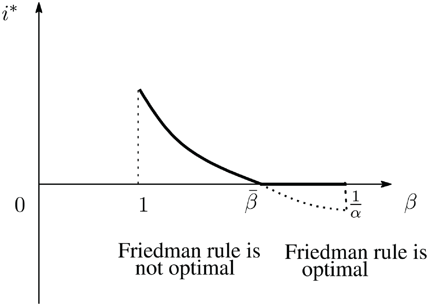
As shown in cases (i) and (ii), if $\bar {\beta }$
is lower, the Friedman rule can be optimal even in the present model where money growth can reduce income tax. For instance, if
$\bar {\beta }$
is lower, the Friedman rule can be optimal even in the present model where money growth can reduce income tax. For instance, if $\nu$
is lower,
$\nu$
is lower, $\bar {\beta }$
is lower, then the Friedman rule tends to be optimal. The reason is as follows.
$\bar {\beta }$
is lower, then the Friedman rule tends to be optimal. The reason is as follows. $\nu$
represents the degree of contribution of R&D to TFP. If
$\nu$
represents the degree of contribution of R&D to TFP. If $\nu$
is lower, the benefit of R&D is lower from social point of view, and thus R&D tends to be eccessive. Hence raising corporate income tax rate and reducing money growth raise welfare.
$\nu$
is lower, the benefit of R&D is lower from social point of view, and thus R&D tends to be eccessive. Hence raising corporate income tax rate and reducing money growth raise welfare.
4.2.2 Numerical examples
We demonstrate the welfare-maximizing nominal interest rate and inflation rate quantitatively. As mentioned above, whether the Friedman rule ( $i=0$
) maximizes welfare or not depends heavily on R&D contribution to TFP
$i=0$
) maximizes welfare or not depends heavily on R&D contribution to TFP $\nu$
. Thus we show the case where
$\nu$
. Thus we show the case where $\nu$
is high and that where it is low.
$\nu$
is high and that where it is low.
First, we assume $\nu =0.25$
, which is relatively high. For the quantitative evaluation, we set the parameters as follows. We set the discount rate
$\nu =0.25$
, which is relatively high. For the quantitative evaluation, we set the parameters as follows. We set the discount rate $\rho$
to
$\rho$
to $0.05$
following Acemoglu and Akcigit (Reference Acemoglu and Akcigit2012). We set
$0.05$
following Acemoglu and Akcigit (Reference Acemoglu and Akcigit2012). We set $\alpha$
to
$\alpha$
to $0.625$
so that the range of patent breadth
$0.625$
so that the range of patent breadth $[1, 1/\alpha ]$
includes
$[1, 1/\alpha ]$
includes $[1.05, 1.4]$
, which is the range of the markup rate estimated by Basu (Reference Basu1996). Following Chu and Wang (Reference Chu and Wang2022), we set the labor income tax to
$[1.05, 1.4]$
, which is the range of the markup rate estimated by Basu (Reference Basu1996). Following Chu and Wang (Reference Chu and Wang2022), we set the labor income tax to $0.238$
. We set the strength of CIA to one and normalize
$0.238$
. We set the strength of CIA to one and normalize $\bar {\ell }=1$
. Finally, we consider
$\bar {\ell }=1$
. Finally, we consider $\beta =1.4$
as a benchmark case and we set
$\beta =1.4$
as a benchmark case and we set $\gamma =1.6$
,
$\gamma =1.6$
, $\ell _G=0.091$
, and
$\ell _G=0.091$
, and $a=0.925$
. By using these values, we can make the ratio of the labor supply to
$a=0.925$
. By using these values, we can make the ratio of the labor supply to $\bar {\ell }$
close to
$\bar {\ell }$
close to $1/3$
, which is a general value by used in earlier studies such as Zheng, Huang, and Yang (2021), and the ratio of government spending to GDP
$1/3$
, which is a general value by used in earlier studies such as Zheng, Huang, and Yang (2021), and the ratio of government spending to GDP $w \ell _G/Y$
close to
$w \ell _G/Y$
close to $0.36$
, which is the value of the US in 2022 reported by the IMF, and the growth rate of output
$0.36$
, which is the value of the US in 2022 reported by the IMF, and the growth rate of output $\nu g_n^\ast$
close to
$\nu g_n^\ast$
close to $1.8 \%$
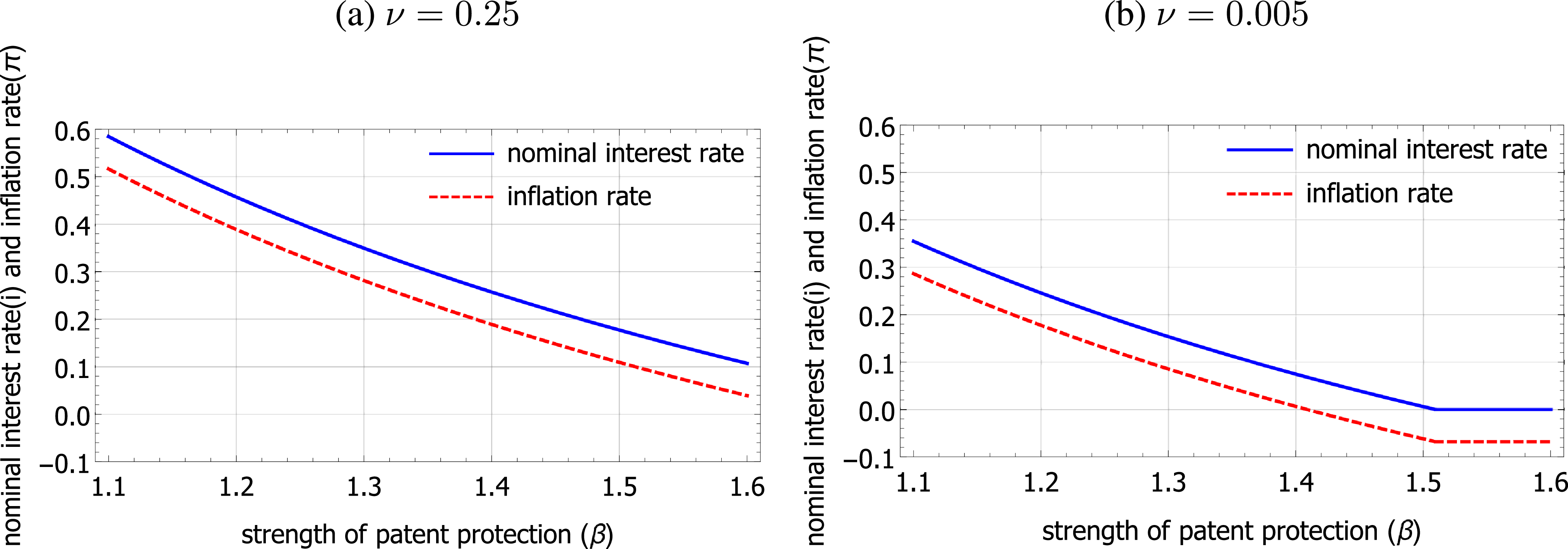
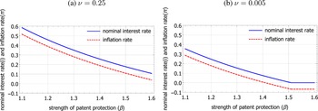
, which is the average growth rate of the US. In this case, the welfare-maximizing nominal interest rate and inflation rate are relatively high as in Panel (a) of Figure 3. Even when the patent protection is so strong that patent breadth is
$1.8 \%$
, which is the average growth rate of the US. In this case, the welfare-maximizing nominal interest rate and inflation rate are relatively high as in Panel (a) of Figure 3. Even when the patent protection is so strong that patent breadth is $1.6$
, the optimal interest rate is positive, namely, the Friedman rule is not optimal.
$1.6$
, the optimal interest rate is positive, namely, the Friedman rule is not optimal.
The welfare-maximizing nominal interest rate and infaltion rate.
Second, we assume $\nu =0.005$
, which is relatively low. Here, in order to make the ratio of the labor supply, the government spending GDP ratio, and the growth rate of output, close to the respective actual values, we set
$\nu =0.005$
, which is relatively low. Here, in order to make the ratio of the labor supply, the government spending GDP ratio, and the growth rate of output, close to the respective actual values, we set $\gamma =1.89$
,
$\gamma =1.89$
, $\ell _G=0.09$
, and
$\ell _G=0.09$
, and $a=0.01835$
. In this case, the welfare-maximizing nominal interest rate and inflation rate are relatively low as in Panel (b) of Figure 3. In particular, when patent protection is so strong that patent breadth is higher than
$a=0.01835$
. In this case, the welfare-maximizing nominal interest rate and inflation rate are relatively low as in Panel (b) of Figure 3. In particular, when patent protection is so strong that patent breadth is higher than $1.5$
, the optimal nominal interest rate is zero, namely, the Friedman rule is optimal.
$1.5$
, the optimal nominal interest rate is zero, namely, the Friedman rule is optimal.
5. Lump-sum tax regime
So far, we assume that the government is unable to employ lump-sum taxation. In this section, we assume that the government is able to employ lump-sum taxation and can set all the distortionary taxes to zero, that is, $\tau _\Pi =\tau _w=0$
. In this case, the government’s budget is given by
$\tau _\Pi =\tau _w=0$
. In this case, the government’s budget is given by $\frac {\dot {M}(t)}{P(t)}+T(t)= w(t) \ell _G$
, and thus, the lump-sum tax
$\frac {\dot {M}(t)}{P(t)}+T(t)= w(t) \ell _G$
, and thus, the lump-sum tax $T(t)$
is determined as
$T(t)$
is determined as $T(t)=w(t)\ell _G-\mu \xi c(t)$
. This means that the seigniorage by money growth only reduces the lump-sum tax. The lump-sum tax has no impact on the resource allocations such as consumption
$T(t)=w(t)\ell _G-\mu \xi c(t)$
. This means that the seigniorage by money growth only reduces the lump-sum tax. The lump-sum tax has no impact on the resource allocations such as consumption $c(t)$
and labor supply
$c(t)$
and labor supply $\ell (t)$
. In this regime, the ratio of consumption to the productivity,
$\ell (t)$
. In this regime, the ratio of consumption to the productivity, $z(t)$
and
$z(t)$
and $\ell (t)$
are determined as follows:Footnote
13
$\ell (t)$
are determined as follows:Footnote
13
 \begin{eqnarray} z^\ast =\frac { \bar {\ell }-\ell _G +a \rho }{\{1 + \gamma [1+\xi (\rho +\mu )] \} \beta }, \end{eqnarray}
 \begin{eqnarray} \ell ^\ast = \bar {\ell } - \gamma [ 1+ \xi (\rho +\mu ) ] \beta z^\ast . \end{eqnarray}
Subsequently, the growth rate of $n(t)$
is as follows.
$n(t)$
is as follows.
 \begin{eqnarray} g_n^\ast = \frac {1}{a} \left [ \ell (t) - \ell _G -z^\ast \right ] = \frac {1}{a} \left ( \bar {\ell } - \ell _G - \left \{ 1+\gamma \beta \left [1+\xi (\rho +\mu ) \right ] \right \} z^\ast \right )\!. \end{eqnarray}
Differentiating (38) with respect to $\mu$
yields
$\mu$
yields
 \begin{align*} \displaystyle \frac {\partial g_n^\ast }{\partial \mu } &= \frac {1}{a} \left ( -\gamma \xi \beta z^\ast - \left \{ 1+\gamma \beta \left [ 1+\xi (\rho +\mu ) \right ] \right \} \frac {\partial z^\ast }{\partial \mu } \right ) \\[6pt] &= -\gamma \xi \beta \frac {z^\ast }{a} \left [ 1- \frac {1+\gamma \beta [1+\xi (\rho +\mu )] }{\{1 + \gamma [1+\xi (\rho +\mu )] \} \beta } \right ] \\[6pt] &= -\gamma \xi \beta \frac {z^\ast }{a} \frac { \beta -1 }{\{ 1+ \gamma [1+\xi (\rho +\mu )] \}\beta }\lt 0. \end{align*}
In the lump-sum tax regime, there is no positive effect on growth, and thus, the growth effect of raising money growth rate is necessarily negative.
Next, we examine the welfare effect of raising money growth rate. The utility of the household is given by (29). Differentiating this with respect to $\mu$
, we obtain
$\mu$
, we obtain
 \begin{eqnarray} \displaystyle \frac {\partial U}{\partial \mu } = \frac {1}{\rho } \Bigl [ \underbrace { (1+\gamma ) \frac {1}{z^\ast } \frac {\partial z^\ast }{\partial \mu } + \gamma \frac {\xi }{ 1+\xi (\rho +\mu )} } _{\stackrel {\mbox{static-allocation effect}}{\mbox{(-)}}} \quad + \quad \underbrace {\frac {1}{\rho } \nu \frac {\partial g_n^\ast }{\partial \mu }} _{\stackrel {\mbox{growth effect}}{\mbox{(-)}}} \Bigr ]. \end{eqnarray}
As is shown before, the growth effect is negative in the lump-sum tax regime. From (36), we can rewrite the term of the static allocation effect as follows.
 \begin{align*} \displaystyle (1+\gamma ) \frac {1}{z^\ast } \frac {\partial z^\ast }{\partial \mu } + \gamma \frac {\xi }{ 1+\xi (\rho +\mu )} &= - (1+\gamma ) \frac {\gamma \xi }{1+\gamma [ 1+\xi (\rho +\mu )]} + \gamma \frac {\xi }{ 1+\xi (\rho +\mu )} \\ &= \gamma \xi \left \{ -\frac {1+\gamma }{1+\gamma [ 1+\xi (\rho +\mu )]} + \frac {1}{ 1+\xi (\rho +\mu )} \right \} \\ &= \gamma \xi \frac {- \xi (\rho +\mu )}{\left \{1+\gamma [ 1+\xi (\rho +\mu )] \right \} [1+\xi (\rho +\mu )]}\lt 0. \end{align*}
Consequently, the static allocation effect is negative also. The total welfare effect of raising money growth rate is negative, and thus, lower money growth rate increases welfare. Therefore, if the nominal interest rate is subject to the zero lower bound, $\mu =-\rho$
maximizes welfare in the lump-sum tax regime.Footnote
14
$\mu =-\rho$
maximizes welfare in the lump-sum tax regime.Footnote
14
6. Conclusion
Governments can reduce income taxes using revenue from issuing new money, that is, seigniorage. Considering this benefit of money growth, this study derives the welfare-maximizing rate of money growth. To examine what types of economies has a high welfare-maximizing money growth rate, we employ a standard R&D-based growth model with endogenous labor supply, in which consumption is subject to a CIA constraint. The most important result is that stronger patent protection reduces the welfare-maximizing growth rate of money. Developed countries have stronger patent protection, whereas developing countries have weaker patent protection; thus, this result implies that developed countries tend to prefer lower inflation rates. In fact, this tendency can be observed; therefore, the present model provides a rationale for the actual tendency.
In this study, to keep the equilibrium as simple as possible, we do not consider a situation in which public spending and investment improve the productivity. It is important to examine the welfare-maximizing rate of money growth and the factors affecting it in a more realistic setting includes public spending and investment. We can incorporate productive public spending into the R&D-based growth model in the same way as in Peretto (Reference Peretto2007b) and Beladi, Chen, Chu, Lai, and Lai (Reference Beladi, Chen, Chu, Lai and Lai2022).Footnote 15 Additionally, to obtain clear and general results, the present model is based on a first-generation endogenous growth model, such as Grossman and Helpman (Reference Grossman and Helpman1991). However, similar results are expected to hold even under a non-scale-effects model, such as those of Jones (Reference Jones1995), Segerstrom (Reference Segerstrom1998), and Peretto (Reference Peretto2007a). These models feature transition to a balanced growth path, whereas first-generation endogenous growth models do not; thus, we must derive the transition path. Nevertheless, by approximating the transition path in the same way as in Judd (Reference Judd1982) and Iwaisako (Reference Iwaisako2020), we may be able to analytically examine the welfare-maximizing rate of money growth. These extensions are beyond the scope of this study but are worth examining.
Supplementary material
The supplementary material for this article can be found at https://doi.org/10.1017/S1365100526101084.
Acknowledgements
An earlier version of this paper was circulated under the title “Effects of patent protection on the optimal mix of inflation and income tax.” The author is deeply grateful to the editor, William A. Barnett, an anonymous associate editor, and two anonymous referees for their helpful comments and suggestions, which have substantially improved the paper. The author gratefully acknowledges the financial support from Japan Center for Economic Research, the Japan Society for the Promotion of Science (JSPS) [grant numbers JP17K03623, JP20K01561, and JP25K05002], and and the Joint Usage/Research Centers at the Institute of Social and Economic Research (ISER) and the Kyoto Institute of Economic Research (KIER). The usual disclaimer applies.
Appendix A: Derivations of the optimality conditions
In this appendix, we derive optimality conditions (3)–(5). We define $\lambda (t)$
and
$\lambda (t)$
and $\lambda _m(t)$
as the costate variables of
$\lambda _m(t)$
as the costate variables of $a(t)$
and
$a(t)$
and $m(t)$
and defined
$m(t)$
and defined $\nu (t)$
as the Kuhn–Tucker multiplier for the CIA constraint. The current-value Hamiltonian
$\nu (t)$
as the Kuhn–Tucker multiplier for the CIA constraint. The current-value Hamiltonian $H$
is given by
$H$
is given by
 \begin{align*} H &\equiv \ln c(t) + \gamma \ln \left [ \bar {\ell } -\ell (t) \right ] \\[4pt] &\quad + \lambda (t) \left [ r(t) a(t) +(1-\tau _w) w(t) \ell (t) -c(t) -\pi (t) m(t) -T(t) -s(t) \right ] \\[4pt] &\quad + \lambda _m(t) s(t) +\nu (t) (m(t)-\xi c(t)). \end{align*}
The optimality conditions are as follows:
 \begin{align} \displaystyle \frac {\partial H}{\partial c(t)}=0 & \,\,\,:\,\,\, \frac {1}{c(t)} = \lambda (t)+ \xi \nu (t) \\[-5pt]\nonumber \end{align}
 \begin{align} \frac {\partial H}{\partial \ell (t)}=0 & \,\,\,:\,\,\, \gamma \frac {1}{\bar {\ell }-\ell (t)} = \lambda (t) (1-\tau _w) w(t) \\[-5pt]\nonumber \end{align}
 \begin{align} \dot {\lambda }(t) - \rho \lambda (t)= -\frac {\partial H}{\partial a(t)} & \,\,\,:\,\,\, \frac {\dot {\lambda }(t)}{\lambda (t)} = \rho - r(t) \\[-5pt]\nonumber\end{align}
 \begin{align} \dot {\lambda }_m(t) - \rho \lambda _m(t)= -\frac {\partial H}{\partial m(t)} & \,\,\,:\,\,\, \frac {\dot {\lambda }_m(t)}{\lambda _m(t)} = \rho + \frac {\lambda (t)}{\lambda _m(t)} \pi (t) -\frac {\nu (t)}{\lambda _m(t)} \nonumber \\ \frac {\partial H}{\partial \lambda (t)}= \dot {a}(t)& \,\,\,:\,\,\, \dot {a}(t)=r(t) a(t) +(1-\tau _w) w(t) \ell (t) -c(t) -\pi (t) m(t) -T(t)-s(t), \nonumber \\ \frac {\partial H}{\partial \lambda _m(t)}= \dot {m}(t)& \,\,\,:\,\,\, \dot {m}(t)=s(t), \\[-5pt]\nonumber\end{align}
 \begin{align} \mbox{Kuhn-Tucker condition}& \,\,\,:\,\,\, \nu (t) (m(t)- \xi c(t))=0, \nonumber \\ \mbox{Transversality conditions}& \,\,\,:\,\,\, \lim _{t \to \infty } e^{-\rho t} \lambda (t) a(t) = 0, \lim _{t \to \infty } e^{-\rho t} \lambda _m(t) m(t) = 0. \end{align}
Additionally, we assume that the change in money holdings $s(t)$
is finite: Subsequently, the equilibrium condition for money holdings is
$s(t)$
is finite: Subsequently, the equilibrium condition for money holdings is
 \begin{eqnarray} \displaystyle \lambda (t)=\lambda _m(t). \end{eqnarray}
By substituting (45) into (43), we obtain $ \frac {\dot {\lambda }(t)}{\lambda (t)} = \rho + \pi (t) -\frac {\nu (t)}{\lambda (t)}$
. Combining this with (42) yields:
$ \frac {\dot {\lambda }(t)}{\lambda (t)} = \rho + \pi (t) -\frac {\nu (t)}{\lambda (t)}$
. Combining this with (42) yields:
 \begin{eqnarray} \displaystyle \nu (t) = \left [ r(t)+\pi (t) \right ] \lambda (t). \end{eqnarray}
This implies that $\nu (t)$
is not zero, and from (44), the CIA constraint is binding:
$\nu (t)$
is not zero, and from (44), the CIA constraint is binding: $m(t)=\xi c(t)$
. By substituting (46) into (40), we obtain (3). Furthermore, by substituting (3) into (41), we obtain (4). We obtain (5) also as shown in (42).
$m(t)=\xi c(t)$
. By substituting (46) into (40), we obtain (3). Furthermore, by substituting (3) into (41), we obtain (4). We obtain (5) also as shown in (42).
Appendix B: The derivation of the equilibrium nominal interest rate
Taking the logarithm of both sides of (3) and differentiating both sides yields
 \begin{eqnarray} \displaystyle -\frac {\dot {c}(t)}{c(t)}=\frac {\dot {\lambda }(t)}{\lambda (t)}+\frac {\xi \dot {i}(t)}{1+\xi i(t)}. \end{eqnarray}
The CIA constraint is binding at each point in time, and thus, $\xi c(t)=m(t)$
. Taking the logarithm of both sides of this equation and differentiating both sides yields
$\xi c(t)=m(t)$
. Taking the logarithm of both sides of this equation and differentiating both sides yields
 \begin{eqnarray*} \displaystyle \frac {\dot {c}(t)}{c(t)}=\frac {\dot {m}(t)}{m(t)}. \end{eqnarray*}
From the definition of $m(t)$
:
$m(t)$
:
 \begin{eqnarray*} \displaystyle \frac {\dot {c}(t)}{c(t)}=\frac {\dot {m}(t)}{m(t)}=\frac {\dot {M}(t)}{M(t)}-\frac {\dot {P}(t)}{P(t)}=\mu -\pi (t). \end{eqnarray*}
By substituting this, (42), and the Fisher equation $i(t)=r(t)+\pi (t)$
into (47), we obtain
$i(t)=r(t)+\pi (t)$
into (47), we obtain
 \begin{eqnarray} \displaystyle \frac {\xi \dot {i}(t)}{1+\xi i(t)}=i(t)-(\rho +\mu ). \end{eqnarray}
The unique positive steady state, $i(t)=\rho +\mu$
, is unstable. Subsequently, the nominal interest rate must jump to this steady state at the initial point in time. Therefore, the nominal interest rate
$i(t)=\rho +\mu$
, is unstable. Subsequently, the nominal interest rate must jump to this steady state at the initial point in time. Therefore, the nominal interest rate $i(t)$
is equal to the constant,
$i(t)$
is equal to the constant, $\rho +\mu$
, from the start.
$\rho +\mu$
, from the start.
Appendix C: Proof of Proposition2: The case where the corporate income tax rate is constant
To derive the direct effect of an increase in the money growth rate on the growth rate, we examine the equilibrium path when the corporate income tax rate is constant, that is, when the government does not lower the tax rate by issuing new money.
By substituting (18) into (22), we obtain the differential equation for $z(t)$
as follows:
$z(t)$
as follows:
 \begin{eqnarray*} \frac {\dot {z}(t)}{z(t)} &=& \left [ 1+(1-\tau _\Pi )(\beta -1) + \gamma \frac {1+\xi (\rho +\mu )}{1-\tau _w}\beta \right ] \frac {\beta }{a}z(t) - \left [\frac {\bar {\ell }-\ell _G}{a} +\rho \right ], \end{eqnarray*}
with a steady state
 \begin{eqnarray} z^\ast = \frac { \bar {\ell }-\ell _G +a \rho }{1+(1-\tau _\Pi )(\beta -1) + \gamma \frac {1+\xi (\rho +\mu )}{1-\tau _w}\beta }. \end{eqnarray}
In the same manner, as in the case in which money growth lowers the tax rate, the steady state is unstable, and the equilibrium path of $z(t)$
is determined by this. The growth rate of
$z(t)$
is determined by this. The growth rate of $n(t)$
is constant and determined as follows:
$n(t)$
is constant and determined as follows:
 \begin{eqnarray} g_n^\ast = \frac {1}{a} \left [ \ell (t) - \ell _G -z^\ast \right ] = \frac {1}{a} \left \{ \bar {\ell } - \ell _G - \left [ 1+\gamma \beta \frac {1+\xi (\rho +\mu )}{1-\tau _w} \right ] z^\ast \right \}. \end{eqnarray}
Differentiating (50) regarding $\mu$
yields
$\mu$
yields
 \begin{align*} \displaystyle \frac {\partial g_n^\ast }{\partial \mu } &= \frac {1}{a} \left [ -\gamma \frac {\xi }{1-\tau _w} \beta z^\ast - \left (\gamma \frac {1+\xi (\rho +\mu )}{1-\tau _w}\beta +1 \right ) \frac {\partial z^\ast }{\partial \mu } \right ] \\[4pt] &= -\gamma \frac {\xi }{1-\tau _w} \beta \frac {z^\ast }{a} \left [ 1- \frac { \gamma \frac {1+\xi (\rho +\mu )}{1-\tau _w}\beta +1 }{1+(1-\tau _\Pi )(\beta -1) + \gamma \frac {1+\xi (\rho +\mu )}{1-\tau _w}\beta } \right ] \\[4pt] &= -\gamma \frac {\xi }{1-\tau _w} \beta \frac {z^\ast }{a} \frac { (1-\tau _\Pi ) (\beta -1) }{1+(1-\tau _\Pi )(\beta -1) + \gamma \frac {1+\xi (\rho +\mu )}{1-\tau _w}\beta }\lt 0. \end{align*}
This shows that an increase in money growth lowers the growth rate of output. Moreover, rewriting this yields:
 \begin{eqnarray} \displaystyle \frac {\partial g_n^\ast }{\partial \mu }= -\gamma \frac {\xi }{1-\tau _w} \beta \frac {z^\ast }{a} \frac { (1-\tau _\Pi ) }{\frac {1}{\beta -1}+(1-\tau _\Pi ) + \gamma \frac {1+\xi (\rho +\mu )}{1-\tau _w} \left ( 1+\frac {1}{\beta -1} \right ) }. \end{eqnarray}
From (49), $\beta z^\ast$
is an increasing function of
$\beta z^\ast$
is an increasing function of $\beta$
. Therefore, an increase in
$\beta$
. Therefore, an increase in $\beta$
increases the absolute value of the RHS of (51). Thus, we show that stronger patent protection strengthens the negative effect of an increase in money growth on output growth rate.
$\beta$
increases the absolute value of the RHS of (51). Thus, we show that stronger patent protection strengthens the negative effect of an increase in money growth on output growth rate.
Appendix D: Proof of Proposition3
Substituting (26) and (32) into (30) and rewriting this yields
 \begin{align*} \displaystyle \frac {\partial U}{\partial \mu } &= \frac {1}{\rho } \Bigr \{ -\frac {(1+\gamma )\xi }{\gamma [1+\xi (\rho +\mu )] +1+\xi \mu } \left [ 1+ \frac {\gamma }{1+\gamma } \frac {\xi \rho }{ 1+\xi (\rho +\mu )} \right ] \\[5pt] &\quad +\frac {1}{\rho } \nu (1+\gamma ) \xi \beta \frac {z^\ast }{a} \frac {\frac {\gamma }{1+\gamma }\frac {1}{1-\tau _w} \xi \rho +\frac {1}{\beta } }{\gamma [1+\xi (\rho +\mu )] +1+\xi \mu } \Bigr \} \\[5pt] &= \frac {1}{\rho } \frac {(1+\gamma )\xi }{\left \{\gamma [1+\xi (\rho +\mu )] +1+\xi \mu \right \}^2} \bigg ( - \Big [ 1+ \frac {\gamma }{1+\gamma } \frac {\xi \rho }{ 1+\xi (\rho +\mu )} \Big ]\left \{\gamma [1+\xi (\rho +\mu )] +1+\xi \mu \right \} \\[5pt] &\quad +\frac {1}{\rho } \nu \beta \frac {z^\ast }{a} \left \{ \gamma [1+\xi (\rho +\mu )] +1+\xi \mu \right \} \Big ( \frac {\gamma }{1+\gamma }\frac {1}{1-\tau _w} \xi \rho +\frac {1}{\beta } \Big ) \bigg ). \end{align*}
Substituting (24) yields
 \begin{align*} \displaystyle \frac {\partial U}{\partial \mu } &= \frac {1}{\rho } \frac {(1+\gamma )\xi }{\left \{\gamma [1+\xi (\rho +\mu )] +1+\xi \mu \right \}^2} \bigg ( - \left [ 1+ \frac {\gamma }{1+\gamma } \frac {\xi \rho }{ 1+\xi (\rho +\mu )} \right ]\left \{\gamma [1+\xi (\rho +\mu )] +1+\xi \mu \right \} \\[6pt] &\quad +\frac {1}{\rho } \nu \left [ (1-\tau _w) \bar {\ell } +\rho \right ] \left ( \frac {\gamma }{1+\gamma }\frac {1}{1-\tau _w} \xi \rho +\frac {1}{\beta } \right ) \bigg ). \end{align*}
Using $\Omega$
, we can rewrite as follows:
$\Omega$
, we can rewrite as follows:
 \begin{align} \displaystyle \frac {\partial U}{\partial \mu } = \frac {1}{\rho } \frac {(1+\gamma )\xi }{ \{ \gamma [1+\xi (\rho +\mu )] +1+\xi \mu \}^2 } \Bigr [ \Omega -(1+\gamma ) -2\gamma \xi \rho -(1+\gamma ) \xi \mu + \frac {\gamma }{1+\gamma } \frac {\xi ^2 \rho ^2}{1+\xi (\rho +\mu )} \Bigr ], \end{align}
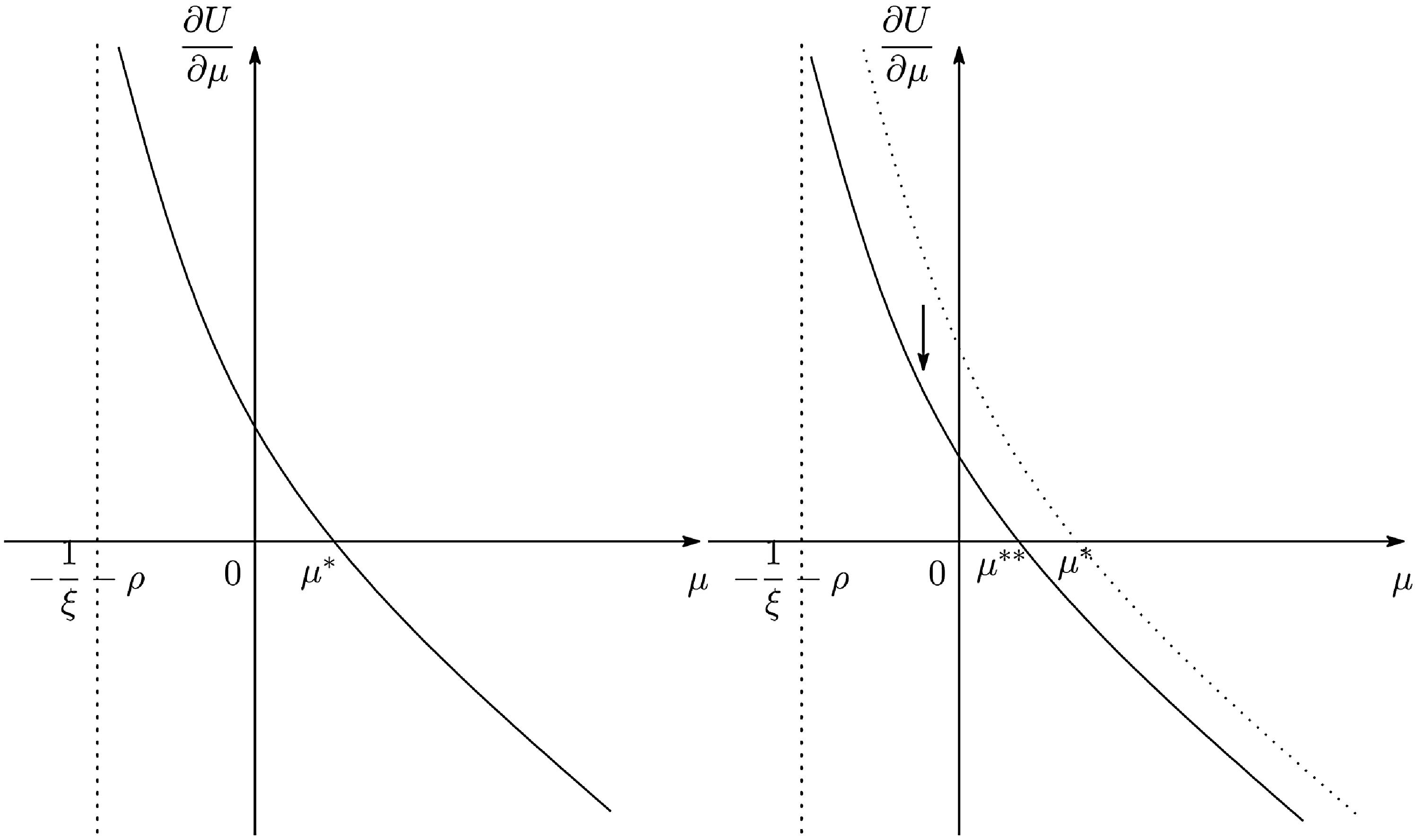
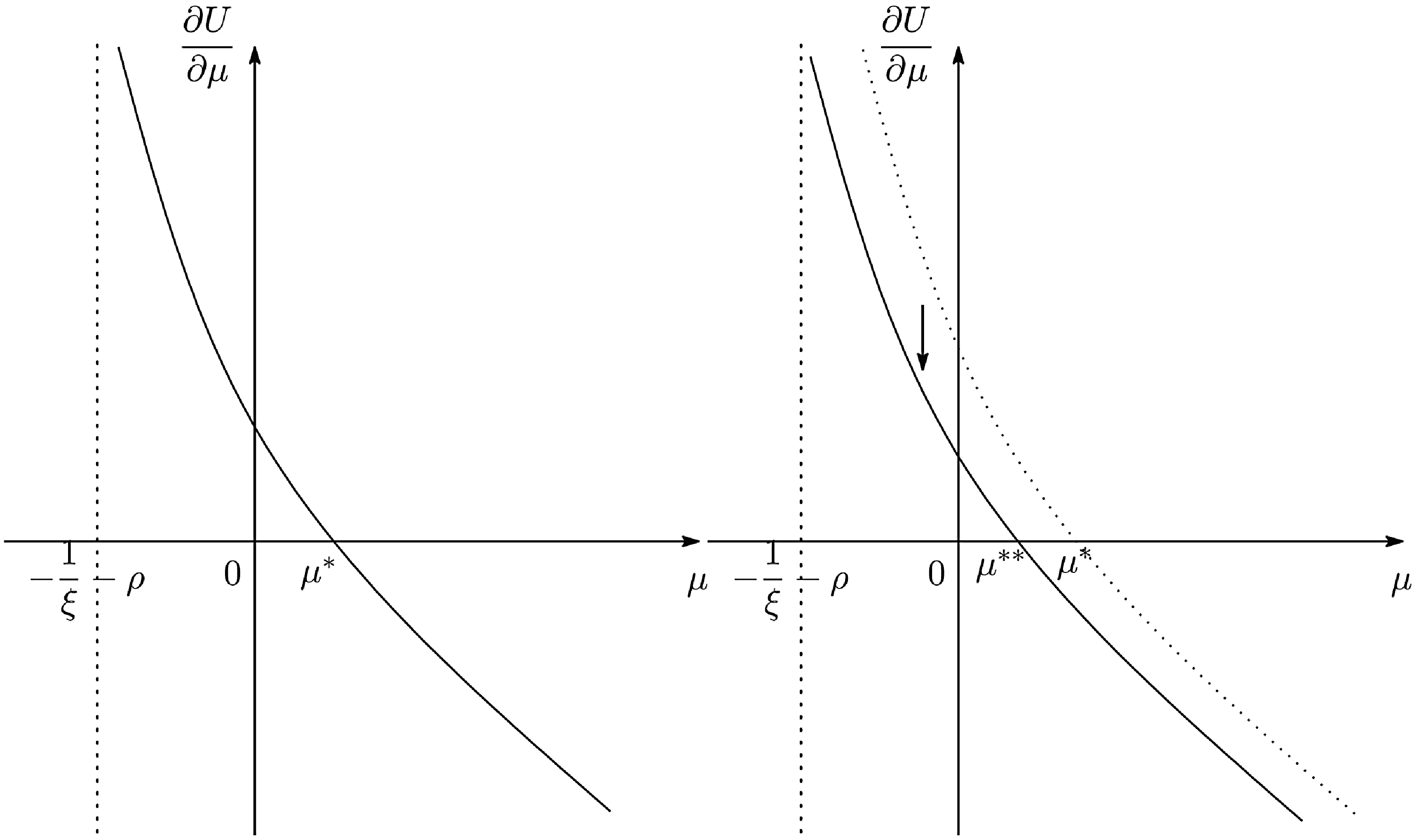
Welfare-maximizing money growth rate.
where $\Omega$
is expressed by (34). The RHS of (52) is a decreasing function of
$\Omega$
is expressed by (34). The RHS of (52) is a decreasing function of $\mu$
, at least if
$\mu$
, at least if $\mu \ge -\frac {1}{\xi }-\rho$
, as shown in the left panel of Figure 4. Thus, there exists a unique value of
$\mu \ge -\frac {1}{\xi }-\rho$
, as shown in the left panel of Figure 4. Thus, there exists a unique value of $\mu$
that satisfies
$\mu$
that satisfies $\frac {\partial U}{\partial \mu } =0$
. We let
$\frac {\partial U}{\partial \mu } =0$
. We let $\mu ^\ast$
denote the value.
$\mu ^\ast$
denote the value. $\frac {\partial U}{\partial \mu }$
is a decreasing function of
$\frac {\partial U}{\partial \mu }$
is a decreasing function of $\mu$
, and thus,
$\mu$
, and thus, $\mu ^\ast$
satisfies the second-order condition. Hence,
$\mu ^\ast$
satisfies the second-order condition. Hence, $\mu ^\ast$
is the welfare-maximizing money growth rate. From (52), the welfare-maximizing condition is given by
$\mu ^\ast$
is the welfare-maximizing money growth rate. From (52), the welfare-maximizing condition is given by
 \begin{eqnarray*} \displaystyle -\Omega +(1+\gamma ) +2\gamma \xi \rho +(1+\gamma ) \xi \mu = \frac {\gamma }{1+\gamma } \frac {\xi ^2 \rho ^2}{1+\xi (\rho +\mu )}. \end{eqnarray*}
We can rewrite this equation as a quadratic equation of $[1+\xi (\rho +\mu )]$
as follows:
$[1+\xi (\rho +\mu )]$
as follows:
 \begin{eqnarray} \displaystyle (1+\gamma ) \left [ 1+\xi (\rho +\mu ) \right ]^2 - \left [ \Omega +(1-\gamma )\xi \rho \right ] \left [ 1+\xi (\rho +\mu ) \right ] -\frac {\gamma }{1+\gamma } \xi ^2 \rho ^2=0. \end{eqnarray}
By solving this equation, we can derive $\mu ^\ast$
analytically, as in (33).
$\mu ^\ast$
analytically, as in (33).
Strengthening patent protections ( $\beta \uparrow$
) decreases
$\beta \uparrow$
) decreases $\Omega$
. Subsequently, the curve of
$\Omega$
. Subsequently, the curve of $\frac {\partial U}{\partial \mu }$
shifts downward, as the right panel of Figure 4 shows, and thus, lowers the welfare-maximizing money growth rate.
$\frac {\partial U}{\partial \mu }$
shifts downward, as the right panel of Figure 4 shows, and thus, lowers the welfare-maximizing money growth rate.
Appendix E: Proof of Proposition4
The nominal interest rate $i (=\mu +\rho )$
cannot be negative. Thus if
$i (=\mu +\rho )$
cannot be negative. Thus if $\frac {\partial U}{\partial \mu } \le 0$
at
$\frac {\partial U}{\partial \mu } \le 0$
at $i=\mu +\rho =0$
,
$i=\mu +\rho =0$
, $i=\mu +\rho =0$
maximizes welfare. From (52), the condition is
$i=\mu +\rho =0$
maximizes welfare. From (52), the condition is
 \begin{eqnarray*} \displaystyle \displaystyle \frac {\partial U}{\partial \mu } \Big |_{\mu =-\rho } &\le & 0 \\ \Omega -(1+\gamma ) +(1-\gamma )\xi \rho + \frac {\gamma }{1+\gamma } \xi ^2 \rho ^2 &\le & 0 \\ \Omega &\le & (1+\gamma ) -(1-\gamma )\xi \rho + \frac {\gamma }{1+\gamma } \xi ^2 \rho ^2, \end{eqnarray*}
where the RHS is positive, if $\rho \lt 1$
. From the definition of
$\rho \lt 1$
. From the definition of $\Omega$
, we obtain
$\Omega$
, we obtain
 \begin{eqnarray*} \displaystyle \beta \ge \bar {\beta }, \end{eqnarray*}
where $\bar {\beta }$
is given by (35).
$\bar {\beta }$
is given by (35).
If $\frac {1}{\alpha } \lt \bar {\beta }$
, from the fact that
$\frac {1}{\alpha } \lt \bar {\beta }$
, from the fact that $\Omega$
is a decreasing function of
$\Omega$
is a decreasing function of $\beta$
, for all values of
$\beta$
, for all values of $\beta$
in
$\beta$
in $(1, \frac {1}{\alpha } ]$
, the following inequality holds:
$(1, \frac {1}{\alpha } ]$
, the following inequality holds:
 \begin{eqnarray*} \displaystyle \Omega -(1+\gamma ) +(1-\gamma )\xi \rho + \frac {\gamma }{1+\gamma } \xi ^2 \rho ^2 &\lt & 0. \end{eqnarray*}
Then, from (52), $\frac {\partial U}{\partial \mu }\lt 0$
at
$\frac {\partial U}{\partial \mu }\lt 0$
at $i=\mu +\rho =0$
. Thus
$i=\mu +\rho =0$
. Thus $i=\mu +\rho =0$
maximizes welfare.
$i=\mu +\rho =0$
maximizes welfare.
In contrast, if $\bar {\beta } \le 1$
,
$\bar {\beta } \le 1$
, $\frac {\partial U}{\partial \mu }\gt 0$
at
$\frac {\partial U}{\partial \mu }\gt 0$
at $i=\mu +\rho =0$
. Thus
$i=\mu +\rho =0$
. Thus $i=\mu +\rho \gt 0$
maximizes welfare.
$i=\mu +\rho \gt 0$
maximizes welfare.
Finally, we examine the case where $1\lt \bar {\beta } \le \frac {1}{\alpha }$
. In this case, if
$1\lt \bar {\beta } \le \frac {1}{\alpha }$
. In this case, if $\beta \ge (\lt ) \bar {\beta }$
,
$\beta \ge (\lt ) \bar {\beta }$
, $\frac {\partial U}{\partial \mu } \le (\!\gt ) 0$
at
$\frac {\partial U}{\partial \mu } \le (\!\gt ) 0$
at $i=\mu +\rho =0$
maximizes welfare.
$i=\mu +\rho =0$
maximizes welfare.















 Open access

