





Nomenclature
- $A$
$A$
-
cross-sectional area
-
${C_{P{\rm{max}}}}$
-
maximum pressure coefficient
-
${D_{{\rm{inj}}}}$
-
diameter of secondary injection port
-
${F_{\rm{j}}}$
-
force due to secondary jet momentum
-
${F_y}$
-
total lateral thrust
-
${F_{{\rm{net}}}}$
-
net externally applied forces on control volume
-
${F_P}$
-
force due to wall pressure
-
$h$
-
characteristic height of secondary injection
-
$M$
-
Mach number
-
$\dot m$
-
mass flow rate
-
$n$
-
surface normal unit vector
-
$P$
-
pressure
-
${P_b}$
-
back-pressure acting on control volume exit face
-
${P_f}$
-
pressure on forward-facing step face
-
$q$
-
dynamic pressure
-
$R$
-
specific gas constant
-
${R_C}$
-
shock hyperbola vertex radius of curvature
-
${R_s}$
-
separation hyperbola vertex radius of curvature
-
$r$
-
radius
-
$T$
-
temperature
-
$U$
-
velocity vector
-
${X_s}$
-
boundary layer separation distance
-
$x$
-
longitudinal axis, aligned with the rocket axis
-
${\alpha _{\rm{n}}}$
-
conical nozzle half-angle
-
$\beta {\rm{'}}$
-
proportionality constant set to 0.062
-
$\gamma$
-
ratio of specific heats
-
${\rm{\Delta }}$
-
bow shock standoff distance
-
$\delta $
-
flow deflection angle for oblique shock wave
-
$\zeta $
-
oblique shock wave angle
-
${\rm{\Theta }}$
-
obstruction local inclination angle
-
$\theta $
-
Mach angle/hyperbola asymptote angle
-
$\rho $
-
density
-
${\rm{\Psi }}$
-
rotation angle


Subscripts and superscripts
- amb
-
ambient conditions
- e
-
exit
- in
-
secondary jet conditions at injection port
- inj
-
secondary injection
- plat
-
plateau region
- s
-
condition at boundary layer separation location
- t
-
stagnation state
- *
-
sonic state
1.0 Introduction
The growing demand to launch payloads into orbit has accelerated the development of high-performance rockets [Reference Messinger, Hill, Quinn, Stannard, Doerksen and Johansen1, Reference Schmierer, Kobald, Tomilin, Fischer and Schlechtriem2]. Modern rockets require enhanced manoeuvrability to perform trajectory corrections, docking, deorbiting, reentry and landing [Reference Sutton and Biblarz3]. Requiring high control authority, thrust vector control (TVC) is used to maintain vehicle flight stability and desired trajectory [Reference Pelouch4]. One method for manipulating thrust direction involves injecting fluid laterally into the nozzle in a method known as secondary injection thrust vector control (SITVC) [Reference Green and McCullough5, Reference Newton6]. SITVC has advantages over conventional TVC mechanisms. It eliminates moving mechanical components associated with movable nozzles and generates higher lateral thrust when compared to cold gas thrusters in vacuum [Reference Hozaki, Gagnon, Mayer, Tromblay and Wu7]. Additionally, SITVC is particularly relevant for hybrid rocket technologies, as the liquid oxidiser may be used for injection, eliminating challenging flex-seal nozzles [Reference Carroll, Cherrington, Greatrix, Harry, Lapp, Porcher, Sokoloff, Spencer, Trumpour and Viechweg8]. Furthermore, it is effective across a wide range of flight regimes, including both atmospheric and vacuum conditions [Reference Sutton and Biblarz3]. Lastly, active flow control via secondary injection shows great potential for use on dual-bell nozzles [Reference Zmijanovic, Leger, Sellam and Chpoun9].
Despite these advantages, accurate prediction of thrust vector generation in SITVC nozzles remains challenging. The injected jet interacts strongly with the supersonic primary flow, producing oblique shocks, bow shocks, boundary layer separation, turbulent vortical structures and highly asymmetric wall pressure distributions that collectively determine the resulting thrust vector. High-fidelity numerical simulations and experiments can resolve these complex interactions, but their computational and experimental cost makes them impractical for rapid design iteration, parametric studies or real-time simulation environments. Reduced-order models therefore remain important engineering tools, offering speed and affordability over experimental and computational techniques. They are also particularly suitable for integration into six degree-of-freedom rocket simulation frameworks.
Early SITVC models largely relied on empirical correlations, correction factors and experimental calibration [Reference Broadwell10–Reference Zukoski and Spaid16]. Rather than serving as standalone predictive frameworks that directly map injectant properties and nozzle geometry to thrust vector outputs, these models required extensive experimental calibration. Moreover, this calibration depended heavily on the specific compositions of both the injectant and the primary rocket motor thrust, leading to models that are not readily generalisable to new propellant-injectant combinations and hindering the reproducibility of results.
Subsequent semi-empirical blunt-body models reduced the dependence on injectant- and propellant-dependent calibration factors, leading to improved generalisability and establishing standalone SITVC prediction frameworks [Reference Maarouf17–Reference Zmijanovic, Leger, Depussay, Sellam and Chpoun20]. By treating the injected secondary jet as an equivalent physical obstruction to the primary supersonic flow, these models could estimate key flow characteristics including boundary layer separation, wall pressure distributions and resultant thrust. However, a critical limitation persisted: the conditions of the secondary jet at the nozzle exit remained unknown, yet were required for determining the effective obstruction geometry. To circumvent this, these frameworks commonly prescribe arbitrary secondary jet exit conditions, or introduce auxiliary assumptions regarding jet behaviour downstream of injection. Such assumptions can introduce substantial deviations from conservation principles, reduce reproducibility and obscure the physical basis of model predictions.
This work develops a new semi-empirical framework for SITVC analysis, termed the mass- and momentum-conserved secondary injection model (MMC-SIM), that removes this closure deficiency. Rather than prescribing the downstream jet state, MMC-SIM determines the equivalent obstruction geometry by simultaneously satisfying mass and momentum conservation constraints on a control volume surrounding the injected jet. This coupled conservation closure yields both the effective injection height and the secondary jet exit condition as part of the solution, providing a physically constrained and transparent analytical framework for thrust vector prediction.
The contributions of this work are as follows:
-
1. A coupled mass-momentum closure formulation is developed for determining the effective obstruction geometry in blunt-body SITVC modelling.
-
2. A fully specified and reproducible implementation is presented, including explicitly solution procedures and governing relations.
-
3. The framework predicts intermediate flow quantities (including separation location and wall pressure distribution) in addition to overall thrust vector characteristics.
-
4. Computational fluid dynamics (CFD) simulations are used to examine dominant flow structures and assess assumptions underlying the MMC-SIM formulation, while model validation is performed against experimental measurements reported in the literature.
The remainder of this paper first reviews existing modelling approaches for SITVC, then presents the MMC-SIM formulation, followed by a limited CFD-based flow analysis used to examine dominant interaction structures and evaluate key modelling assumptions, before validation against available experimental data.
2.0 Background on modelling of SITVC
Secondary injection thrust vector control generates lateral force through coupled momentum addition and pressure-induced loading on the nozzle wall. Figure 1 schematically illustrates the key flow phenomena responsible for lateral thrust generation in an SITVC nozzle and is adapted from Fig. 1 in Ref. (Reference Balu, Marathe, Paul and Mukunda21). Following injection, the secondary jet interacts strongly with the supersonic primary flow, producing an upstream separation shock, a bow shock enveloping the injected jet, boundary layer separation and a highly asymmetric wall pressure distribution. In addition to direct momentum injection by the secondary jet, this pressure asymmetry contributes substantially to lateral force generation and overall thrust vectoring performance.
Schematic of key flow features generated by secondary injection thrust vector control.

Figure 1. Long description
A diagram illustrating the flow features generated by secondary injection thrust vector control. The diagram shows a cross-sectional view of a flow system with various labeled components and features. The primary supersonic flow enters from the left and interacts with a secondary sonic jet injected perpendicularly. Key features include the bow shock, jet boundary, recirculation zone, and separation shock. The primary supersonic flow is deflected by the secondary sonic jet, creating a complex interaction region. The bow shock forms ahead of the jet boundary, while the separation shock occurs where the primary flow separates. The recirculation zone is located downstream of the secondary sonic jet, indicating a region of reversed flow. The diagram also highlights the interaction between the secondary jet and the primary flow, showing how the jet momentum affects the overall flow dynamics.
The complex three-dimensional flow involves shock-wave/boundary-layer interaction, turbulent mixing, jet expansion and recirculation regions [Reference Huang22, Reference Zhang, McCreton, Awasthi, Wills, Moreau and Doolan23]. Accurate first-principles analytical modelling of the full interaction field is therefore intractable. Instead, predictive models simplify the flow physics while retaining the mechanisms most influential to thrust generation.
Most analytical SITVC models combine theoretical analysis with empirical correlations to estimate these quantities [Reference Pelouch4, Reference Wilson and Comparin14]. Their differences primarily lie in how the equivalent obstruction is defined, how wall pressure distributions are represented and how the secondary jet state is modelled. These distinctions give rise to several broad classes of analytical models, reviewed in the following section.
A central unresolved challenge across reduced-order SITVC modelling is the closure of the secondary jet interaction problem. The effective obstruction geometry and downstream jet state are not directly known, yet both strongly influence predicted separation behaviour, wall pressure loading and ultimately thrust vector magnitude. Existing approaches typically address this uncertainty through prescribed jet exit conditions or empirical scaling relations. The accuracy and reproducibility of model predictions therefore depend strongly on how this closure problem is treated.
The modelling framework developed in this work focuses specifically on this closure problem. By determining the effective obstruction geometry through simultaneous enforcement of mass and momentum conservation, MMC-SIM replaces prescribed downstream assumptions with a physically constrained closure while retaining the computational efficiency of semi-empirical blunt-body modelling.
Recent advances in computational and experimental investigations have substantially improved the understanding of SITVC flow physics. Modern numerical and experimental studies have investigated parameters affecting thrust vector performance and flow structures within an SITVC nozzle [Reference Chen and Liao24–Reference Younes, Grenke, Hickey, Gagnon and Elzein31]. These investigations provide increasingly detailed characterisation of asymmetric pressure loading, shock interaction and vortex dynamics associated with fluidic thrust vectoring. Despite these advances, comparatively few recent developments have focused on reduced-order analytical modelling, where closure of the jet-flow interaction remains a persistent challenge. As a result, analytical and semi-empirical models continue to play an important role in rapid engineering prediction, preliminary design and reduced-order simulation environments.
2.1 Overview of models in the literature
Early analytical modelling efforts established much of the conceptual foundation for SITVC analysis. Wu et al. [Reference Wu, Chapkis and Mager15] set an early benchmark by applying conservation of mass, momentum and energy to describe secondary injection interactions. However, the complexity of the jet-freestream interaction required substantial simplifications, limiting the model’s ability to accurately predict thrust vector behaviour and resolve intermediate flow features such as separation location or wall pressure distribution. Moreover, this framework relied on experimentally derived scaling parameters dependent on the injectant. This dependence means experiments are required for each exhaust-injectant interaction, significantly hindering widespread use of this approach.
Experimental investigations by Zukoski and Spaid [Reference Zukoski and Spaid16] later provided important physical insight into the interaction field using Schlieren visualisation. Their observations showed that the injected jet behaves as an effective obstruction to the primary flow, producing a bow shock and upstream flow separation analogous to flow over a blunt body. This led to the development of ‘blunt-body’ analogies for SITVC modelling, where the secondary jet is represented by an equivalent obstruction in the primary flow. Prediction of the thrust generated in an SITVC nozzle using the blunt-body approach involves three main steps:
-
1. Determination of an equivalent obstruction, usually using the characteristic height,
$h$
-
2. Prediction of the resulting wall pressure distribution in the vicinity of the injection port
-
3. Calculation of the net thrust vector by combining wall pressure and jet momentum contributions

This framework remains attractive because it provides prediction not only of overall thrust, but also of intermediate flow quantities directly linked to vectoring performance.
Subsequent models progressively improved the representation of the wall pressure field. Wilson et al. [Reference Wilson and Comparin14] introduced one of the first semi-empirical formulations that explicitly partitioned the wall pressure distribution into distinct flow regions. Later, Mangin [Reference Mangin18] and Maarouf [Reference Maarouf17] extended the blunt-body approach to axisymmetric nozzles by developing a more complete semi-empirical framework for predicting separation location, pressure loading and thrust vector generation. For brevity, this work refers to this modelling family as the Evry model . Subsequent studies attempted to reproduce the model, but had to introduce additional assumptions and simplifications to address problem closure [Reference Chen and Liao24, Reference Deng, Kong and Kim32, Reference Younes and Hickey33]. More recently, Younes et al. [Reference Younes and Hickey33] conducted a sensitivity analysis. Of note, they highlight the importance of accurately estimating the shock position and that reliance on empirical relations may introduce additional error.
Despite their usefulness, existing blunt-body formulations share an important modelling limitation: closure of the effective obstruction problem is typically achieved by prescribing unknown downstream jet conditions or by introducing auxiliary assumptions regarding jet geometry or exit behaviour. These quantities are not generally known a priori, and as such, the resulting closure can introduce significant deviations from conservation consistency and can make implementation sensitive to modelling assumptions.
This limitation is distinct from the broader use of empirical relations in semi-empirical modelling, which remain valuable for representing difficult-to-model flow phenomena. Rather, the unresolved issue is that the effective obstruction geometry, which fundamentally governs separation distance and wall pressure loading, is often determined through assumed downstream conditions rather than through physically constrained closure.
MMC-SIM builds directly on the blunt-body modelling tradition while addressing this specific limitation. Instead of prescribing the downstream jet state, the equivalent obstruction height is determined as part of the solution through simultaneous satisfaction of mass and momentum conservation constraints. This preserves the interpretability and computational efficiency of reduced-order blunt-body modelling while strengthening its physical consistency and reproducibility.
3.0 Modelling of SITVC
3.1 Overview of MMC-SIM
Building on these foundational works [Reference Wu, Chapkis and Mager15, Reference Maarouf17, Reference Mangin18, Reference Spaid and Zukoski34, Reference Zukoski35], a semi-empirical model was developed to compute the thrust vector for three-dimensional converging-diverging nozzles. The MMC-SIM framework enforces both mass and momentum conservation, avoiding the need for other assumptions seen in subsequent models.
MMC-SIM predicts the thrust vector in an SITVC nozzle by modelling the secondary jet as an equivalent blunt body with a quarter-sphere nose of radius $h$
, referred to as the injection height. Traditional blunt-body models determine this characteristic dimension,
$h$
, referred to as the injection height. Traditional blunt-body models determine this characteristic dimension, $h$
, by balancing drag against assumed jet exit momentum, which requires prescribing unknown secondary jet exit conditions [Reference Zukoski and Spaid16, Reference Maarouf17, Reference Deng, Kong and Kim32]. MMC-SIM removes this assumption by formulating the equivalent obstruction height as a coupled closure problem: conservation of mass and conservation of momentum provide two independent constraints that are solved simultaneously for both the jet exit state and the corresponding injection height. This enables the determination of the effective obstruction geometry without prescribing downstream jet conditions a priori.
$h$
, by balancing drag against assumed jet exit momentum, which requires prescribing unknown secondary jet exit conditions [Reference Zukoski and Spaid16, Reference Maarouf17, Reference Deng, Kong and Kim32]. MMC-SIM removes this assumption by formulating the equivalent obstruction height as a coupled closure problem: conservation of mass and conservation of momentum provide two independent constraints that are solved simultaneously for both the jet exit state and the corresponding injection height. This enables the determination of the effective obstruction geometry without prescribing downstream jet conditions a priori.
3.1.1 Complexity of SITVC flow structures
The three-dimensional flow structure produced by SITVC is inherently complex, involving a horseshoe vortex, a pair of counter-rotating vortices, mixing between the jet and freestream, and recirculation zones. Detailed analytical modelling of these individual phenomena and their interactions is challenging. Instead, the model can be greatly simplified if only the features that contribute significantly to the thrust vector are considered. These features of interest, including the adverse pressure gradient and boundary layer separation, lie near the nozzle wall and may be approximated using a combination of analytical modelling and empirical relations.
3.1.2 Modelling simplifications and assumptions
MMC-SIM applies the blunt-body analogy and the following assumptions for thrust vector predictions:
-
1. The secondary jet is deflected by the primary freestream until it is parallel to the nozzle wall.
-
2. The equivalent body has a quarter-sphere nose.
-
3. No mixing occurs between the primary and secondary flows.
-
4. Shear stresses on the control volume are negligible.
-
5. The boundary layer thickness is much less than the injection height.
3.1.3 MMC-SIM architecture
MMC-SIM consists of two subroutines. Using the nozzle geometry and flow properties as inputs, the first subroutine calculates the injection height, $h$
, and the boundary layer separation position,
$h$
, and the boundary layer separation position, ${x_s}$
. These intermediate results are passed to the second subroutine, which determines the thrust by numerically integrating the pressure along the nozzle wall. Full details of each subroutine are provided in Sections 3.2 and 3.3. A more detailed implementation of the MMC-SIM algorithm, including full source code and supporting derivations, is provided in the author’s thesis [Reference Abdelwahab36].
${x_s}$
. These intermediate results are passed to the second subroutine, which determines the thrust by numerically integrating the pressure along the nozzle wall. Full details of each subroutine are provided in Sections 3.2 and 3.3. A more detailed implementation of the MMC-SIM algorithm, including full source code and supporting derivations, is provided in the author’s thesis [Reference Abdelwahab36].
3.2 Subroutine 1: injection height determination
A control volume encompassing the secondary jet is shown in Fig. 2 based on Fig. 6 from Ref. (Reference Zmijanovic, Lago, Leger, Depussay, Sellam and Chpoun37). The centre of the secondary injection port is located at ${x_{{\rm{inj}}}}$
. Note that the nozzle divergence (half-angle) is assumed to be small and is neglected. The oncoming primary flow is deflected through the oblique shock upstream of the obstruction by the turning angle,
${x_{{\rm{inj}}}}$
. Note that the nozzle divergence (half-angle) is assumed to be small and is neglected. The oncoming primary flow is deflected through the oblique shock upstream of the obstruction by the turning angle, $\delta $
. The onset of boundary layer separation occurs at
$\delta $
. The onset of boundary layer separation occurs at ${x_s}$
.
${x_s}$
.
Control volume encompassing equivalent body with quarter-sphere nose.

The boundary layer separation distance, ${X_s}$
, which describes the distance from the separation position to the injection port, is defined by assuming that the deflected flow is tangential to the quarter-sphere nose according to Equation (1).
${X_s}$
, which describes the distance from the separation position to the injection port, is defined by assuming that the deflected flow is tangential to the quarter-sphere nose according to Equation (1).
 \begin{align}{X_s} \approx h\left( {\frac{1}{{{\rm{sin}}\delta }} - 1} \right) \end{align}
Note that Equation (1) neglects the thickness of the jet. The boundary layer separation position, ${x_s}$
, is determined using Equation (2).
${x_s}$
, is determined using Equation (2).
 \begin{align}{x_s} = {x_{{\rm{inj}}}} - {X_s} \end{align}
Experimental investigations of supersonic flow over forward-facing steps conducted by Zukoski [Reference Zukoski35] showed that the pressure within the separated region may be approximated as constant. This so-called plateau pressure, ${P_{{\rm{plat}}}}$
, is primarily dictated by the freestream deflection angle,
${P_{{\rm{plat}}}}$
, is primarily dictated by the freestream deflection angle, $\delta $
. Jet-induced separation exhibits similar behaviour. However, given that the obstacle size generated by the jet is unknown, empirical relations are used to estimate the plateau pressure from the primary flow properties at
$\delta $
. Jet-induced separation exhibits similar behaviour. However, given that the obstacle size generated by the jet is unknown, empirical relations are used to estimate the plateau pressure from the primary flow properties at ${x_s}$
. The static pressure of the freestream after the oblique shock,
${x_s}$
. The static pressure of the freestream after the oblique shock, ${P_{{\rm{plat}}}}$
is computed using the empirical relation proposed by Zukoski and given in Equation (3) [Reference Zukoski35]:
${P_{{\rm{plat}}}}$
is computed using the empirical relation proposed by Zukoski and given in Equation (3) [Reference Zukoski35]:
 \begin{align}{P_{{\rm{plat}}}} = {P_s}\left( {0.5{M_s} + 1} \right) \end{align}
Subscript $s$
indicates primary flow properties at the separation position,
$s$
indicates primary flow properties at the separation position, ${x_s}$
.
${x_s}$
.
A further increase in pressure occurs immediately upstream of the obstruction. Equation (4) is used to estimate the pressure acting on the upstream face of the obstruction, ${P_f}$
. The proportionality constant
${P_f}$
. The proportionality constant $\beta {\rm{'}}$
was set to 0.062 based on experimental force measurements reported by Zukoski [Reference Zukoski35] for supersonic transverse injection configurations. Although treating
$\beta {\rm{'}}$
was set to 0.062 based on experimental force measurements reported by Zukoski [Reference Zukoski35] for supersonic transverse injection configurations. Although treating $\beta {\rm{'}}$
as a tunable parameter could potentially improve agreement with numerical simulations or experiments, such an optimisation is beyond the scope of the present work and is left for future investigation. Moreover, the pressure on the upstream face of the control volume does not show dependence on
$\beta {\rm{'}}$
as a tunable parameter could potentially improve agreement with numerical simulations or experiments, such an optimisation is beyond the scope of the present work and is left for future investigation. Moreover, the pressure on the upstream face of the control volume does not show dependence on $\beta {\rm{'}}$
if the obstacle height is larger than the boundary layer thickness.
$\beta {\rm{'}}$
if the obstacle height is larger than the boundary layer thickness.
 \begin{align}{P_f} = {P_{{\rm{plat}}}}\left( {1 + \beta {\rm{'}}\frac{{\gamma M_{{\rm{plat}}}^2}}{{1 + \frac{{\gamma - 1}}{2}M_{{\rm{plat}}}^2}}} \right) \end{align}
The pressure ratio across the oblique shock, ${P_{{\rm{plat}}}}/{P_s}$
, is used to find the shock angle,
${P_{{\rm{plat}}}}/{P_s}$
, is used to find the shock angle, $\zeta $
, and the flow deflection angle according to Equations (5) and (6) [Reference John and Keith38].
$\zeta $
, and the flow deflection angle according to Equations (5) and (6) [Reference John and Keith38].
 \begin{align}{\rm{sin}}\zeta = \sqrt {\frac{{\frac{P{_{{\rm{plat}}}}}{{{P_s}}}\left( {\gamma + 1} \right) + \left( {\gamma - 1} \right)}}{{2\gamma M_s^2}}} \end{align}
 \begin{align}{\rm{tan}}\delta = {\rm{cot}}\zeta \frac{{M_s^2{\rm{si}}{{\rm{n}}^2}\zeta - 1}}{{\frac{{\gamma + 1}}{2}M_s^2 - \left( {M_s^2{\rm{si}}{{\rm{n}}^2}\zeta - 1} \right)}} \end{align}
Finally, the Mach number of the freestream flow after the oblique shock is obtained from Equation (7) [Reference John and Keith38].
 \begin{align}M_{{\rm{plat}}}^2{\rm{si}}{{\rm{n}}^2}\left( {\delta - \zeta } \right) = \frac{{\left( {\gamma - 1} \right)M_s^2{\rm{si}}{{\rm{n}}^2}\delta + 2}}{{2\gamma M_s^2{\rm{si}}{{\rm{n}}^2}\delta - \left( {\gamma - 1} \right)}} \end{align}
3.2.1 Conservation of mass
The secondary mass flow into the control volume is known and is defined by the secondary injection port flow conditions as follows:
 \begin{align}{\dot m_{{\rm{in}}}} = \int\!\!\!\int \rho U \cdot ndA = {\rho _{{\rm{in}}}}{U_{{\rm{in}}}}{A_{{\rm{port}}}} \end{align}
where the subscript ‘in’ denotes secondary jet conditions at the injection port with area ${A_{{\rm{port}}}}$
. Assuming that no mixing occurs between the primary and secondary flows, the mass flow rates entering and exiting the control volume are equal by conservation of mass.
${A_{{\rm{port}}}}$
. Assuming that no mixing occurs between the primary and secondary flows, the mass flow rates entering and exiting the control volume are equal by conservation of mass.
 \begin{align}{\dot m_{\rm{j}}} = {\dot m_{{\rm{in}}}} = {\dot m_{\rm{e}}} \end{align}
Additionally, the mass flow rate across the exit face is expressed using stagnation properties as follows:
 \begin{align}{\dot m_{\rm{e}}} = \frac{{{P_{{\rm{tj}}}}}}{{\sqrt {{T_{{\rm{tj}}}}} }}{A_{\rm{e}}}{M_{{\rm{j}},{\rm{e}}}}\sqrt {\frac{{{\gamma _{\rm{j}}}}}{{{R_{\rm{j}}}}}} {\left( {1 + \frac{{{\gamma _{\rm{j}}} - 1}}{2}M_{{\rm{j}},{\rm{e}}}^2} \right)^{ - \frac{{{\gamma _{\rm{j}}} + 1}}{{2\left( {{\gamma _{\rm{j}}} - 1} \right)}}}} \end{align}
Subscript ‘j’ indicates secondary jet properties. Note that the exit area of the control volume is assumed to be a half-circle with radius $h$
.
$h$
.
 \begin{align}{A_{\rm{e}}} = \frac{\pi }{2}{h^2} \end{align}
Rearranging Equation (10) yields an expression for the injection height derived from conservation of mass, as shown in Equation (12).
 \begin{align}{h_{{\rm{mass}}}} = {\left[ {\sqrt {{{{R_{\rm{j}}}} \over {{\gamma _{\rm{j}}}}}} {2 \over {{M_{{\rm{j}},{\rm{e}}}}\pi }}{{\sqrt {{T_{tj}}} } \over {{P_{tj}}}}{{\dot m}_{\rm{j}}}{{\left( {1 + {{{\gamma _{\rm{j}}} - 1} \over 2}M_{{\rm{j}},{\rm{e}}}^2} \right)}^{{{{\gamma _{\rm{j}}} + 1} \over {2\left( {{\gamma _{\rm{j}}} - 1} \right)}}}}} \right]^{{1 \over 2}}} \end{align}
Note that the subscript ‘mass’ indicates that the height is derived from a conservation of mass assumption. Equation (12) establishes the first constraint on the injection height, $h$
. However, the jet exit conditions (specifically Mach number,
$h$
. However, the jet exit conditions (specifically Mach number, ${M_{{\rm{j}},{\rm{e}}}}$
) remain unknown. All other parameters in this equation are known.
${M_{{\rm{j}},{\rm{e}}}}$
) remain unknown. All other parameters in this equation are known.
3.2.2 Conservation of momentum
Applying momentum conservation yields the second constraint on the injection height. The net force in the $x$
-direction,
$x$
-direction, $\Sigma {F_x}$
, is balanced by the momentum of the exiting jet,
$\Sigma {F_x}$
, is balanced by the momentum of the exiting jet, ${\dot m_{\rm{e}}}{V_{{\rm{j}},{\rm{e}}}}$
, as established in Equation (13).
${\dot m_{\rm{e}}}{V_{{\rm{j}},{\rm{e}}}}$
, as established in Equation (13).
 \begin{align}\sum {F_x} = {F_{x1}} + {F_{x2}} = {\dot m_{\rm{j}}}{V_{{\rm{j}},{\rm{e}}}} \end{align}
Here, ${F_{x1}}$
and
${F_{x1}}$
and ${F_{x2}}$
represent the
${F_{x2}}$
represent the $x$
-components of the forces on the upstream and downstream faces of the control volume, respectively. To evaluate
$x$
-components of the forces on the upstream and downstream faces of the control volume, respectively. To evaluate ${F_{x1}}$
, the pressure on the upstream face of the control volume is integrated.
${F_{x1}}$
, the pressure on the upstream face of the control volume is integrated.
 \begin{align}{F_{x1}} = \int\!\!\!\int P{\rm{sin\Theta sin\Phi }}d{A_{{\rm{upstream}}}} \end{align}
The differential area over a quarter sphere is illustrated in Fig. 3 (based on Fig. 1.30 in Ref. (Reference Rowlands39)) and is calculated according to Equation (15). Angles ${\rm{\Theta }}$
and
${\rm{\Theta }}$
and ${\rm{\Phi }}$
are defined as illustrated in the figure.
${\rm{\Phi }}$
are defined as illustrated in the figure.
 \begin{align}d{A_{{\rm{upstream}}}} = {h^2}{\rm{sin\Theta }}d{\rm{\Theta }}d{\rm{\Phi }} \end{align}
Schematic of area integration over a quarter sphere.

Applying the modified Newtonian theory [Reference Lees40], the pressure on an inclined blunt body is calculated according to Equation (16):
 \begin{align}P = {q_{{\rm{plat}}}}{C_{P{\rm{max}}}}{\rm{si}}{{\rm{n}}^2}{\rm{\Theta si}}{{\rm{n}}^2}{\rm{\Phi }} + {P_{{\rm{plat}}}} \end{align}
Here, ${C_{P{\rm{max}}}}$
is the maximum pressure coefficient defined according to Modified Newtonian Theory [Reference Anderson41]. It is evaluated in the plateau region using Equation (17).
${C_{P{\rm{max}}}}$
is the maximum pressure coefficient defined according to Modified Newtonian Theory [Reference Anderson41]. It is evaluated in the plateau region using Equation (17).
 \begin{align}{C_{P{\rm{max}}}} = \frac{2}{{\gamma M_{{\rm{plat}}}^2}}\left[ {\dfrac{{{{\left( {\dfrac{{\gamma + 1}}{2}M_{{\rm{plat}}}^2} \right)}^{\frac{\gamma }{{\gamma - 1}}}}}}{{{{\left( {\dfrac{{2\gamma }}{{\gamma + 1}}M_{{\rm{plat}}}^2 - \dfrac{{\gamma - 1}}{{\gamma + 1}}} \right)}^{\frac{1}{{\gamma - 1}}}}}} - 1} \right] \end{align}
Substituting Equations (15) and (16) into Equation (14) yields the following:
 \begin{align}{F_{x1}} = \mathop \int \nolimits_0^\pi \mathop \int \nolimits_0^{\pi /2} \left( {{q_{{\rm{plat}}}}{C_{P{\rm{max}}}}{\rm{si}}{{\rm{n}}^2}{\rm{\Theta si}}{{\rm{n}}^2}{\rm{\Phi }} + {P_{{\rm{plat}}}}} \right){h^2}{\rm{si}}{{\rm{n}}^2}{\rm{\Theta sin\Phi }}d{\rm{\Theta }}d{\rm{\Phi }} \end{align}
Evaluating the integral yields Equation (19) for the pressure force on the upstream face of the control volume.
 \begin{align}{F_{x1}} = \frac{\pi }{2}{h^2}\left( {\frac{1}{2}{q_{{\rm{plat}}}}{C_{P{\rm{max}}}} + {P_{{\rm{plat}}}}} \right) \end{align}
Next, the force acting on the downstream face of the control volume may be determined using Equation (20).
 \begin{align}{F_{x2}} = \int PdA = - {\pi \over 2}{h^2}{P_b} \end{align}
Here, ${P_b}$
is the back-pressure acting on the downstream control volume face, which equals the undisturbed nozzle exit pressure,
${P_b}$
is the back-pressure acting on the downstream control volume face, which equals the undisturbed nozzle exit pressure, ${P_{\rm{e}}}$
. Lastly, Equation (21) provides the exiting jet momentum.
${P_{\rm{e}}}$
. Lastly, Equation (21) provides the exiting jet momentum.
 \begin{align}{\dot m_{\rm{j}}}{V_{{\rm{j}},{\rm{e}}}} = {\dot m_{\rm{j}}}{M_{{\rm{j}},{\rm{e}}}}\sqrt {{\gamma _{\rm{j}}}{R_{\rm{j}}}\frac{{{T_{{\rm{tj}}}}}}{{1 + \dfrac{{{\gamma _{\rm{j}}} - 1}}{2}M_{{\rm{j}},{\rm{e}}}^2}}} \end{align}
Combining Equations (19), (20) and (21) yields a relation for the injection height derived from conservation of momentum:
 \begin{align}{h_{{\rm{momentum}}}} = {\left[ {{2 \over \pi }{{{{\dot m}_{\rm{j}}}{M_{{\rm{j}},{\rm{e}}}}\sqrt {{\gamma _{\rm{j}}}{R_{\rm{j}}}{T_{{\rm{j}},{\rm{e}}}}} } \over {{1 \over 2}{q_{{\rm{plat}}}}{C_{P{\rm{max}}}} + {P_{{\rm{plat}}}} - {P_{\rm{b}}}}}} \right]^{1/2}} \end{align}
Note that the subscript ‘momentum’ indicates that the height is derived from a conservation of momentum assumption. As in the equation derived from continuity, the jet exit condition remains unknown ( ${M_{{\rm{j}},{\rm{e}}}},{T_{{\rm{j}},{\rm{e}}}}$
). All other parameters in Equation (22) are known.
${M_{{\rm{j}},{\rm{e}}}},{T_{{\rm{j}},{\rm{e}}}}$
). All other parameters in Equation (22) are known.
3.2.3 Numerical implementation of the coupled solution procedure
Figure 4 outlines the numerical implementation of the coupled closure procedure used to determine the injection height.
Numerical implementation workflow for coupled conservation closure in MMC-SIM.

An initial estimate of the injection height, ${h_i}$
, is used to determine the shock separation location and corresponding primary flow properties. Using these quantities, the plateau pressure and flow turning characteristics are evaluated, allowing the plateau-region flow properties to be determined. The coupled mass and momentum conservation equations are then solved simultaneously for the updated injection height,
${h_i}$
, is used to determine the shock separation location and corresponding primary flow properties. Using these quantities, the plateau pressure and flow turning characteristics are evaluated, allowing the plateau-region flow properties to be determined. The coupled mass and momentum conservation equations are then solved simultaneously for the updated injection height, ${h_{i + 1}}$
, and jet exit Mach number,
${h_{i + 1}}$
, and jet exit Mach number, ${M_{j,e}}$
. These nonlinear conservation equations were solved simultaneously using the MATLAB® fzero root-finding routine. Specifically, the root,
${M_{j,e}}$
. These nonlinear conservation equations were solved simultaneously using the MATLAB® fzero root-finding routine. Specifically, the root, ${M_{{\rm{j}},{\rm{e}}}}$
, satisfies the following condition:
${M_{{\rm{j}},{\rm{e}}}}$
, satisfies the following condition:
 \begin{align}{h_{{\rm{mass}}}} - {h_{{\rm{momentum}}}} = 0 \end{align}
The procedure is repeated iteratively until the relative change in injection height between successive iterations satisfies
 \begin{align*}\frac{{\left| {{h_{i + 1}} - {h_i}} \right|}}{{{h_i}}} \lt 0.01\% . \end{align*}
Following convergence, the final separation location is recomputed using the converged injection height.
3.3 Subroutine 2: force determination
The nozzle thrust is composed of the primary and secondary jet momentum contributions and the wall pressure contributions. The wall pressure distribution is divided into three distinct regions, as illustrated in Fig. 5: (I) undisturbed nozzle at ${P_{{\rm{isen}}}}$
, (II) separated region at
${P_{{\rm{isen}}}}$
, (II) separated region at ${P_{{\rm{plat}}}}$
and (III) elevated pressure region at
${P_{{\rm{plat}}}}$
and (III) elevated pressure region at ${P_{\rm{f}}}$
.
${P_{\rm{f}}}$
.
Wall pressure distribution schematic in vicinity of secondary injection for conical nozzle.

Figure 5. Long description
A diagram of the cross-sectional area and pressure distribution in the vicinity of secondary injection for a conical nozzle. The diagram includes various labeled parts and relationships. The throat is located at the top, with the separation curve and bow shock curve indicated. The diagram is divided into three regions labeled I, II, and III. Key elements include the throat, separation curve, bow shock curve, and various directional arrows indicating flow and pressure distribution. The diagram also shows the characteristic height of secondary injection, Mach number, mass flow rate, surface normal unit vector, pressure, back-pressure acting on the control volume exit face, pressure on the forward-facing step face, dynamic pressure, specific gas constant, shock hyperbola vertex radius of curvature, separation hyperbola vertex radius of curvature, radius, temperature, velocity vector, boundary layer separation distance, longitudinal axis, conical nozzle half-angle, proportionality constant, ratio of specific heats, bow shock standoff distance, flow deflection angle for oblique shock wave, oblique shock wave angle, obstruction, local inclination angle, Mach angle/hyperbola asymptote angle, density, and rotation angle.
The thrust vector may be broken up into the axial and lateral components, denoted ${F_x}$
and
${F_x}$
and ${F_y}$
, respectively. The
${F_y}$
, respectively. The $x$
-component is parallel to the rocket axis, while the
$x$
-component is parallel to the rocket axis, while the $y$
-component is perpendicular. They are calculated according to Equations (24) and (25), respectively.
$y$
-component is perpendicular. They are calculated according to Equations (24) and (25), respectively.
 \begin{align}{F_x} = {F_{x,{\rm{throat}}}} + {F_{x,P}} - {P_{{\rm{amb}}}}{A_{\rm{e}}} \end{align}
 \begin{align}{F_y} = {F_{y,{\rm{jet}}}} + {F_{y,P}} \end{align}
Here, ${F_{x,{\rm{throat}}}}$
and
${F_{x,{\rm{throat}}}}$
and ${F_{y,{\rm{jet}}}}$
are the primary jet momentum at the nozzle throat, and the secondary jet momentum at the injector port, respectively.
${F_{y,{\rm{jet}}}}$
are the primary jet momentum at the nozzle throat, and the secondary jet momentum at the injector port, respectively. ${F_{x,P}}$
and
${F_{x,P}}$
and ${F_{y,P}}$
represent the
${F_{y,P}}$
represent the $x$
- and
$x$
- and $y$
-components of the force due to the asymmetric wall pressure distribution, respectively. The primary jet momentum is calculated at the throat as shown in Equation (26):
$y$
-components of the force due to the asymmetric wall pressure distribution, respectively. The primary jet momentum is calculated at the throat as shown in Equation (26):
 \begin{align}{F_{x,{\rm{throat}}}} = \dot m{V_{{\rm{throat}}}} + {P_{{\rm{throat}}}}{A_{{\rm{throat}}}} \end{align}
For a secondary jet injected perpendicular to the nozzle axis, the momentum contributions to the thrust are calculated according to Equation (27):
 \begin{align}{F_{y,{\rm{jet}}}} = {\dot m_{\rm{j}}}{V_{\rm{j}}} + \left( {{P_{\rm{j}}} - {P_{\infty ,x{\rm{IP}}}}} \right){A_{{\rm{port}}}} \end{align}
Here, ${P_{\rm{j}}}$
and
${P_{\rm{j}}}$
and ${P_{\infty ,x{\rm{IP}}}}$
are the pressure of the secondary jet at the injection port, and the pressure of the undisturbed primary flow at the injection port plane, respectively. Numerical integration of the pressure over the nozzle wall is performed to obtain the pressure contributions,
${P_{\infty ,x{\rm{IP}}}}$
are the pressure of the secondary jet at the injection port, and the pressure of the undisturbed primary flow at the injection port plane, respectively. Numerical integration of the pressure over the nozzle wall is performed to obtain the pressure contributions, ${F_{x,P}}$
and
${F_{x,P}}$
and ${F_{y,P}}$
.
${F_{y,P}}$
.
3.3.1 Pressure contribution to the thrust vector
Given a continuous pressure distribution on an area, the force vector may be determined using Equation (28).
 \begin{align}{F_P} = \int PndA \end{align}
However, the pressure distribution over the nozzle wall is discretised into a grid of cells, each defined by indices $m$
and
$m$
and $n$
, corresponding to the
$n$
, corresponding to the $x$
-axial and
$x$
-axial and ${\rm{\Psi }}$
-angular positions, respectively. Numerical integration is performed over these discrete cells to approximate the total pressure contribution across the surface. In Equation (28), the unit outward normal,
${\rm{\Psi }}$
-angular positions, respectively. Numerical integration is performed over these discrete cells to approximate the total pressure contribution across the surface. In Equation (28), the unit outward normal, $n$
, is defined by rotating the vector
$n$
, is defined by rotating the vector $\left( {0,1,0} \right)$
by the nozzle half-angle,
$\left( {0,1,0} \right)$
by the nozzle half-angle, ${\alpha _{\rm{n}}}$
, about the
${\alpha _{\rm{n}}}$
, about the $z$
-axis, and by
$z$
-axis, and by ${\psi _n}$
about the
${\psi _n}$
about the $x$
-axis. Thus, the unit outward normal of each cell with index
$x$
-axis. Thus, the unit outward normal of each cell with index $n$
is calculated using Equation (29):
$n$
is calculated using Equation (29):
 \begin{align}{n_n} = \left[ {\begin{array}{c@{\quad}c@{\quad}c}1 {}&0& {}0\\0& {}{{\rm{cos}}{\psi _n}}& {}{ - {\rm{sin}}{\psi _n}}\\0& {}{{\rm{sin}}{\psi _n}}& {}{{\rm{cos}}{\psi _n}}\end{array}} \right]\left[ {\begin{array}{c@{\quad}c@{\quad}c}{{\rm{cos}}{\alpha _n}}& {}0& {}{{\rm{sin}}{\alpha _n}}\\0& {}1& {}0\\{ - {\rm{sin}}{\alpha _n}}& {}0& {}{{\rm{cos}}{\alpha _n}}\end{array}} \right]\left[ {\begin{array}{*{20}{l}}0\\1\\0\end{array}} \right] \end{align}
From Fig. 5, the cell area is calculated using the nozzle radius, ${r_m}$
, according to Equation (30):
${r_m}$
, according to Equation (30):
 \begin{align}d{S_m} = {r_m}d{\rm{\Psi }}dx \end{align}
The force on each cell, indexed by $\left( {m,n} \right),$
is calculated using Equation (31):
$\left( {m,n} \right),$
is calculated using Equation (31):
 \begin{align}d{F_{P,mn}} = {P_m}{n_n}{r_m}d{\rm{\Psi }}dx \end{align}
The overall force vector due to the wall pressure distribution, ${F_P}$
, is calculated by summing over the nozzle length
${F_P}$
, is calculated by summing over the nozzle length $L$
for index
$L$
for index $m$
, and the full angular range of
$m$
, and the full angular range of ${360^ \circ }$
for index
${360^ \circ }$
for index $n$
, as follows:
$n$
, as follows:
 \begin{align}{F_P} = \mathop \sum \limits_m \mathop \sum \limits_n {P_{mn}}{n_n}{r_m}d{\rm{\Psi }}dx \end{align}
The pressure distribution on each $\left( {m,n} \right)$
-indexed cell is elliptically interpolated between the undisturbed nozzle pressure and the pressure of each region (
$\left( {m,n} \right)$
-indexed cell is elliptically interpolated between the undisturbed nozzle pressure and the pressure of each region ( ${P_{{\rm{plat}}}}$
or
${P_{{\rm{plat}}}}$
or ${P_f}$
) as shown in Equation (33).
${P_f}$
) as shown in Equation (33).
 \begin{align}{P_{mn}} = {P_{m,{\rm{isen}}}} + \left( {{P_{m,{\rm{isen}}}} - {P_{{\rm{region}}}}} \right)\sqrt {1 - {{\left( {\frac{{{\psi _n}{r_m}}}{{{\psi _{m,{\rm{max}}}}{r_m}}}} \right)}^2}} \end{align}
Here, ${\psi _{m,{\rm{max}}}}$
describes the angular position of each region boundary, as described in the following section.
${\psi _{m,{\rm{max}}}}$
describes the angular position of each region boundary, as described in the following section.
3.3.2 Region boundaries on the nozzle wall
The nozzle wall is separated into three distinct regions in order to define the pressure distribution as shown in Fig. 5. These regions are delineated by the bow shock curve and the separation curve, as illustrated in three dimensions in Fig. 6(a). The shock shape around a spherical obstruction was predicted to be hyperbolic by Billig [Reference Billig42].
Building on this theory, Maarouf [Reference Maarouf17] proposed that the boundary layer separation profile is also hyperbolic. Using these theories, the shock and separation curves are assumed to have hyperbolic profiles that are asymptotic with the freestream Mach angle, $\theta $
. The Mach angle is evaluated using Equation (34) at the boundary layer separation position,
$\theta $
. The Mach angle is evaluated using Equation (34) at the boundary layer separation position, ${x_s}$
.
${x_s}$
.
 \begin{align}{\rm{sin}}\theta = \frac{1}{{{M_s}}} \end{align}
A two-dimensional slice is shown in Fig. 6b to define ${\psi _{{\rm{max}}}}$
with respect to the
${\psi _{{\rm{max}}}}$
with respect to the $z$
-coordinates of the shock and separation hyperbolas. At each
$z$
-coordinates of the shock and separation hyperbolas. At each $x$
-position slice (indexed
$x$
-position slice (indexed $m$
),
$m$
), ${\psi _{{\rm{max}}}}$
is evaluated using Equation (35).
${\psi _{{\rm{max}}}}$
is evaluated using Equation (35).
 \begin{align}{\rm{tan}}{\psi _{m,{\rm{max}}}} = \frac{{{z_m}}}{{{r_m}}} \end{align}
Figure 7 illustrates the hyperbolic shock and separation profiles ahead of a spherical-nosed body with radius, $h$
, based on Ref. (Reference Billig42). The
$h$
, based on Ref. (Reference Billig42). The $x$
-coordinates of the centre of the injection port and focus point of the hyperbolas are
$x$
-coordinates of the centre of the injection port and focus point of the hyperbolas are ${x_{{\rm{inj}}}}$
and
${x_{{\rm{inj}}}}$
and ${x_F}$
, respectively. The shock standoff distance,
${x_F}$
, respectively. The shock standoff distance, ${\rm{\Delta }}$
, and vertex radius of curvature,
${\rm{\Delta }}$
, and vertex radius of curvature, ${R_C},$
are also illustrated. The final shock and separation hyperbolas are presented in Equations (36) and (37), respectively:
${R_C},$
are also illustrated. The final shock and separation hyperbolas are presented in Equations (36) and (37), respectively:
 \begin{align}{\left[ {\frac{{x - \left( {{x_{{\rm{inj}}}} - {\rm{\Delta }} - {R_C}{\rm{co}}{{\rm{t}}^2}\theta } \right)}}{{{R_C}{\rm{co}}{{\rm{t}}^2}\theta }}} \right]^2} - {\left[ {\frac{{{z_{{\rm{shock}}}}}}{{{R_C}{\rm{cot}}\theta }}} \right]^2} = 1 \end{align}
 \begin{align}{\left[ {\frac{{x - \left( {{x_{c}} - {R_s} - {R_s}{\rm{co}}{{\rm{t}}^2}\theta } \right)}}{{{R_s}{\rm{co}}{{\rm{t}}^2}\theta }}} \right]^2} - {\left[ {\frac{{{z_{{\rm{sep}}}}}}{{{R_s}{\rm{cot}}\theta }}} \right]^2} = 1 \end{align}
(a) Separation and shock hyperbolas on three-dimensional nozzle surface. (b) Schematic of ${\psi _{m,{\rm{max}}}}$
for two-dimensional slice of the nozzle at index
${\psi _{m,{\rm{max}}}}$
for two-dimensional slice of the nozzle at index $m$
.
$m$
.

Schematics of hyperbolic shock and separation profiles generated by a spherical-nosed body.

Lastly, the radius of curvature for the separation curve, ${R_s}$
, may be calculated from the focus point,
${R_s}$
, may be calculated from the focus point, ${x_F}$
according to Equations (38) and (39).
${x_F}$
according to Equations (38) and (39).
 \begin{align}{x_F} = {x_{{\rm{inj}}}} - {\rm{\Delta }} + {R_C} \end{align}
 \begin{align}\kern-2.2pc {R_s} = {x_F} - {x_s} \end{align}
The boundary layer separation position, ${x_s}$
, was determined in subroutine 1.
${x_s}$
, was determined in subroutine 1.
3.3.3 Numerical implementation procedure for the thrust vector
Using the separation position from subroutine 1, the bow shock separation curves are computed, allowing the nozzle wall to be separated into three distinct pressure regions. The pressure distribution is calculated, and the pressure-driven force contribution is determined by integrating along the nozzle wall. The overall thrust vector is calculated by summing the pressure and jet momentum contributions. The procedure to solve for the thrust vector is schematically shown in Fig. 8.
Numerical implementation procedure for thrust vector computation.

4.0 Supporting CFD analysis
Three-dimensional CFD simulations were performed using OpenFOAM [Reference Weller, Tabor, Jasak and Fureby43] with the pimpleCentralFOAM solver [Reference Kraposhin, Bovtrikova and Strijhak44, Reference Kraposhin, Banholzer, Pfitzner and Marchevsky45] to examine dominant flow structures associated with secondary injection in supersonic nozzle flow. The simulations were intended to provide qualitative and semi-quantitative insight into separation behaviour, pressure development, and jet structure relevant to MMC-SIM assumptions, rather than to establish a standalone high-fidelity validation campaign.
A structured mesh with near-wall refinement was employed, and a three-level mesh refinement study was conducted to assess discretisation sensitivity. The medium mesh (5.2 m cells) was selected as a compromise between computational cost and solution variation. Additional details regarding mesh generation and boundary conditions, and verification are provided in Appendix A.
5.0 Problem setup
The geometry and flow properties were selected based on availability of three-dimensional SITVC experimental data in the literature, enabling validation of the model predictions. The simulation parameters, including nozzle geometry and flow conditions, were selected based on the experiments performed at the National Centre for Scientific Research Institute for Combustion, Aerothermics, Reactivity and Environment (ICARE) [Reference Sellam, Chpoun, Zmijanovic and Lago19, Reference Chpoun, Sellam, Zmijanovic and Leger46–Reference Zmijanovic, Lago, Sellam and Chpoun49], herein referred to as the University of Evry experiments. The experimental setup consisted of a blow-down supersonic wind tunnel supplying clean, oil-free, unheated air to both the primary and secondary jets through an SITVC conical nozzle, which exhausted into a vacuum chamber. Experimental setup details are reported by the authors with some discrepancies between the various papers [Reference Sellam, Chpoun, Zmijanovic and Lago19, Reference Zmijanovic, Leger, Depussay, Sellam and Chpoun20, Reference Zmijanovic, Lago, Leger, Depussay, Sellam and Chpoun37, Reference Zmijanovic, Lago, Sellam and Chpoun49]. The nozzle geometry and stagnation temperature were matched to the latest paper [Reference Zmijanovic, Leger, Depussay, Sellam and Chpoun20]. The experimental data used for comparison with the results in this work are from the earlier three papers [Reference Sellam, Chpoun, Zmijanovic and Lago19, Reference Zmijanovic, Lago, Leger, Depussay, Sellam and Chpoun37, Reference Zmijanovic, Lago, Sellam and Chpoun49], as the latest paper does not report the data required. The conical nozzle geometry used is presented in Table 1. This geometry yields a half-angle and area ratio of approximately 5.87° and 4.234, respectively. Given the potential inconsistencies between the simulation inputs and the experimental setup, errors are expected to arise.
Conical nozzle geometry

Table 1. Long description
A table detailing conical nozzle geometry dimensions. The table has six rows and two columns. The first column lists the dimensions: Throat radius, Exit radius, Nozzle length, Injector port position, and Injector port diameter. The second column provides the corresponding values in millimeters: 9.72, 20.0, 100.0, 90.0, and 6.15.
The centre of the injection port is located at 90% of the nozzle length ( ${x_{{\rm{inj}}}} = 90.0$
mm). Note that the origin of the
${x_{{\rm{inj}}}} = 90.0$
mm). Note that the origin of the $x$
-coordinate is set at the nozzle throat. The injection is perpendicular to the primary rocket axis, not the conical nozzle wall. Both primary and secondary flows are air (with a molar mass of 28.96 kg/kmol) at a stagnation pressure of 260 K and an inlet Mach of 1. The primary flow has a stagnation pressure of 300 kPa.
$x$
-coordinate is set at the nozzle throat. The injection is perpendicular to the primary rocket axis, not the conical nozzle wall. Both primary and secondary flows are air (with a molar mass of 28.96 kg/kmol) at a stagnation pressure of 260 K and an inlet Mach of 1. The primary flow has a stagnation pressure of 300 kPa.
The secondary jet stagnation pressure is varied to evaluate its effect on TVC performance. The secondary pressure ratio (SPR) is defined in Equation (40) as the stagnation pressure ratio of the secondary to the primary jets. Analytical and numerical simulations are performed at SPR values of 0.667, 0.833, 1 and 1.167.
 \begin{align}{\rm{SPR}} = \frac{{{P_{{\rm{tj}}}}}}{{{P_{\rm{t}}}}} \end{align}
The SITVC nozzle exhausts into a vacuum chamber with air at an ambient temperature and pressure of 290 K and 8 kPa, respectively.
6.0 Results
This section first presents supporting CFD analysis used to examine dominant SITVC flow structures and assess assumptions underlying MMC-SIM. Experimental comparisons are then used to evaluate predictive performance of the analytical framework.
6.1 Overview of the interaction field
A qualitative analysis of the CFD simulations offers significant insights into the flow features within an SITVC nozzle. Figure 9 presents the streamlines of the flow near the secondary injection port.
Streamlines of two opposing vortices upstream of injector.

Figure 9. Long description
A heat map represents the x-component of velocity in a fluid flow. The color scale ranges from -380 to 600, with colors transitioning from yellow to dark blue. The heat map shows the boundary layer separation, PUV, and SUV regions. The boundary layer separation is indicated by a distinct change in the flow pattern. The PUV and SUV regions are marked with triangles and show different flow characteristics. The x-axis and y-axis are labeled, and the flow patterns are visually distinct with varying intensities of color indicating different velocities.
Upstream of the secondary gas injection, boundary layer separation occurs, creating two distinct counter-rotating vortices in the plateau region. The primary upstream vortex (PUV), which rotates counter-clockwise, occupies the larger portion of the separation zone, while the secondary upstream vortex (SUV) rotates clockwise.
The primary nozzle flow accelerates in the undisturbed region as expected. At the secondary injection port, the jet is introduced sonically, rapidly expanding and accelerating into the primary flow. The Mach number distribution in Fig. 10 provides a detailed view of the regions directly around the injection port. Here, the plateau flow is subsonic upstream of the injection site, a result of the secondary jet obstructing and deflecting the primary nozzle flow. This deflection occurs via two main mechanisms: an oblique separation shock generated upstream of the injection point, and a bow shock surrounding the jet.
Distribution of the Mach number in an SITVC nozzle in the injector port region.

Downstream of the injection, a distinct subsonic region forms, marked by some degree of backflow. This region is associated with extremely low static pressures, lower than the ambient back pressure, creating conditions that allow external flow to re-enter the nozzle. This low-pressure zone, strongly influenced by the stagnation pressure of the external atmosphere, is detrimental to thrust vectoring performance. By driving backflow into the nozzle, it counteracts the desired redirection of thrust, and minimising this low-pressure region is crucial for improving overall vectoring efficiency.
The secondary jet does not reattach to the nozzle wall following injection. Instead, the flow remains detached, suggesting that the jet expansion and interactions with the primary flow prevent reattachment under the current conditions. This detachment impacts the effective direction and magnitude of the thrust vector, highlighting areas for potential improvement in future SITVC nozzle designs aimed at optimising reattachment and minimising backflow zones for enhanced control authority.
This observation also reveals a limitation in MMC-SIM and similar blunt-body models, which assume the secondary gas deflects parallel to the nozzle wall. However, CFD analysis shows that the jet may remain partially detached under certain conditions. Future work could refine the control volume by incorporating a more accurate representation of the equivalent obstruction, based on this detached flow pattern.
6.2 Secondary jet shape
Figure 11 presents cross-sections of traced secondary jet streamlines taken at various $x$
-positions along the nozzle. Observations reveal that the jet continues to expand at least to the exit face of the nozzle. Additionally, each cross-section has non-uniform pressure and density distributions. The cross-sectional shape of the jet is difficult to pinpoint, but more closely approximates an elliptical area than a semi-circular one.
$x$
-positions along the nozzle. Observations reveal that the jet continues to expand at least to the exit face of the nozzle. Additionally, each cross-section has non-uniform pressure and density distributions. The cross-sectional shape of the jet is difficult to pinpoint, but more closely approximates an elliptical area than a semi-circular one.
(a)–(e) Cross-sections of secondary jet streamlines with corresponding nozzle wall at various $x$
-positions. (f) Cross-sections within the three-dimensional nozzle.
$x$
-positions. (f) Cross-sections within the three-dimensional nozzle.

Figure 11. Long description
Panel A: A scatter plot showing secondary jet streamlines at x = 87 mm. The y-axis represents y-Position in meters, and the x-axis represents z-Position in meters. The streamlines are depicted in blue. Panel B: A scatter plot showing secondary jet streamlines at x = 90 mm. The y-axis represents y-Position in meters, and the x-axis represents z-Position in meters. The streamlines are depicted in orange. Panel C: A scatter plot showing secondary jet streamlines at x = 93 mm. The y-axis represents y-Position in meters, and the x-axis represents z-Position in meters. The streamlines are depicted in yellow. Panel D: A scatter plot showing secondary jet streamlines at x = 96 mm. The y-axis represents y-Position in meters, and the x-axis represents z-Position in meters. The streamlines are depicted in purple. Panel E: A scatter plot showing secondary jet streamlines at x = 99 mm. The y-axis represents y-Position in meters, and the x-axis represents z-Position in meters. The streamlines are depicted in green. Panel F: A 3D visualization of the cross-sections within the nozzle, showing the streamlines from panels A to E in their respective colors.
These observations reinforce the difficulty of prescribing downstream jet geometry or exit conditions a priori, as is commonly required in existing blunt-body formulations. MMC-SIM avoids this dependence by determining the effective obstruction height through coupled conservation constraints rather than through assumed downstream jet structure.
6.3 Boundary layer separation
To compare the boundary layer separation positions from MMC-SIM predictions and CFD simulations, the boundary layer separation position is defined as the location of zero wall shear stress ( ${\tau _{\rm{w}}} = 0$
). For the case of SPR
${\tau _{\rm{w}}} = 0$
). For the case of SPR $ = 1.000$
, the CFD simulation results indicate that separation occurs at an
$ = 1.000$
, the CFD simulation results indicate that separation occurs at an $x$
-position of 75.5 mm. Using Equation (1) results in a separation standoff distance of
$x$
-position of 75.5 mm. Using Equation (1) results in a separation standoff distance of ${X_s} = 14.5$
mm. The CFD-derived separation location indicates that MMC-SIM captures the correct upstream separation trend and order of magnitude, despite the simplified equivalent-obstruction representation. Compared to the MMC-SIM prediction of 16.46 mm, this yields a 13.5% error. Table 2 summarises separation standoff distances across various SPR values, with an average error of 14.8% when compared to CFD results. Additionally, Fig. 12 compares the separation standoff distances between MMC-SIM analyses and CFD results.
${X_s} = 14.5$
mm. The CFD-derived separation location indicates that MMC-SIM captures the correct upstream separation trend and order of magnitude, despite the simplified equivalent-obstruction representation. Compared to the MMC-SIM prediction of 16.46 mm, this yields a 13.5% error. Table 2 summarises separation standoff distances across various SPR values, with an average error of 14.8% when compared to CFD results. Additionally, Fig. 12 compares the separation standoff distances between MMC-SIM analyses and CFD results.
Comparison of separation standoff distance results

Table 2. Long description
A table comparing separation standoff distances for different SPR values using MMC-SIM and CFD methods. The table has four rows and three columns. The columns are labeled SPR, MMC-SIM (mm), CFD (mm), and % Error. The rows present the following data: Row 1: SPR, 0.667; MMC-SIM, 15.29; CFD, 12.9; % Error, 18.5%. Row 2: SPR, 0.833; MMC-SIM, 15.89; CFD, 13.6; % Error, 16.9%. Row 3: SPR, 1.000; MMC-SIM, 16.46; CFD, 14.5; % Error, 13.5%. Row 4: SPR, 1.167; MMC-SIM, 16.98; CFD, 15.4; % Error, 10.2%.
Comparison of separation distance as a function of SPR between MMC-SIM analyses and CFD results.

Furthermore, the separation position predicted by the Evry model for the SPR = 1 case was provided by Dr. Sellam (personal communication, October 20, 2023) as 84 mm. This yields a separation distance of 6 mm – considerably shorter than that predicted by CFD.
Qualitative comparisons between the analytically and numerically determined separation curves are illustrated in Fig. 13. The CFD-derived separation curves show localised fluctuations near the separation boundary but preserve the overall topology and upstream trend.
Comparison between boundary layer separation curves determined by MMC-SIM and CFD simulations on nozzle wall.

Overall, the MMC-SIM code over-predicts the separation distance, with the predicted separation point occurring further upstream than observed in CFD simulations. Additionally, the shape of the separation curve generated by the MMC-SIM code follows a narrower, hyperbolic profile, compared to the broader curve produced by the CFD results. Such differences highlight a potential area for refinement of the MMC-SIM code, particularly in better representing the separation curve’s profile to improve the accuracy of thrust vector predictions.
These comparisons are intended to assess whether MMC-SIM captures the dominant separation behaviour associated with SITVC interactions, rather than to establish exact correspondence with the CFD solution.
6.4 Pressure profile
The CFD-derived pressure profile along the wall at 0°, illustrated in Fig. 14, provides insight into the pressure contribution represented within MMC-SIM. As is typical of expanding nozzle flows, the pressure decreases as the flow progresses. Around 72 mm, the adverse pressure gradient begins to develop, as indicated by a reversal in the pressure trend. At some point, the adverse pressure triggers boundary layer separation. The pressure reaches its first peak in the plateau region with a maximum value of 30.9 kPa. Ahead of the secondary injection port, there is a noticeable second pressure spike, reaching 51.5 kPa, as the flow encounters the bow shock. Beyond this, the pressure sharply increases, reaching the secondary jet inlet pressure, before sharply decreasing. The pressure drop downstream of the obstruction indicates the presence of localised backflow created by ambient air entering the nozzle.
Numerically generated wall pressure distribution for SITVC nozzle operating with SPR = 1 for ${\rm{\Psi }} = 0^\circ $
.
${\rm{\Psi }} = 0^\circ $
.

Figure 15 further illustrates how the pressure along the nozzle wall evolves with increasing angular position, ${\rm{\Psi }}$
. The plot reveals an attenuated effect, where the influence of the secondary jet diminishes with increasing distance from the injection point.
${\rm{\Psi }}$
. The plot reveals an attenuated effect, where the influence of the secondary jet diminishes with increasing distance from the injection point.
Numerically generated wall pressure distribution for SITVC nozzle operating with SPR = 1 for various angles, ${\rm{\Psi }}$
.
${\rm{\Psi }}$
.

Next, the pressure profiles generated using CFD simulations and MMC-SIM are compared for various angles, as illustrated in Fig. 16. Both profiles exhibit a similar trend, showing an initial pressure decrease, followed by an increase ahead of the obstruction. This is consistent with flow behaviour in a supersonic nozzle with a lateral jet injection. While the magnitudes are similar, the numerically obtained pressure profile is systematically higher than that of the analytical model in the undisturbed region. The pressure profiles for other SPR values behave similarly. Overall, MMC-SIM reproduces the dominant pressure-rise and separation trends observed in the CFD results.
Comparison of CFD and analytical wall pressure distributions at various angles for SPR = 1.

Figure 16. Long description
Six line graphs compare numerical and MMC-SIM pressure distributions at various angles. Each graph plots pressure in Pascals on the vertical axis against x-position in meters on the horizontal axis. The angles vary from 0 to 135 degrees. Panel A shows the pressure distribution at 0 degrees, Panel B at 15 degrees, Panel C at 45 degrees, Panel D at 60 degrees, Panel E at 90 degrees, and Panel F at 135 degrees. Each graph includes two lines: a solid blue line representing numerical data and a dashed orange line representing MMC-SIM data. The pressure distributions show varying trends and peaks across different angles.
6.5 Thrust vectoring
The primary validation of MMC-SIM is performed through comparison with experimentally measured thrust vector data from the University of Evry SITVC experiments. Particular emphasis is placed on assessing whether the coupled mass-momentum closure improves the prediction of pressure-driven lateral force while retaining the computational simplicity of reduced-order blunt-body modelling in Fig. 17.
The thrust vector predictions produced by MMC-SIM are analysed as a function of SPR. Tables 3 and 4 compare the thrust vector results generated by MMC-SIM with experimental measurements, accompanied by calculated percent errors. MMC-SIM yields average errors of 3.3% in predicting total lateral thrust, and 3.2% in estimating the thrust vector deflection angle.
Validation of MMC-SIM thrust vector with experimental data [Reference Sellam, Chpoun, Zmijanovic and Lago19]

Table 3. Long description
The table compares experimental and simulated thrust vector data with percent errors. It has six columns and four rows. The columns are labeled SPR, Fy (N) Exp, Fy (N) MMC-SIM, Fy (N) % Error, Fx (N) Exp, Fx (N) MMC-SIM, Fx (N) % Error. The rows present the following data: Row 1: SPR 0.667, Fy (N) Exp 12.4, Fy (N) MMC-SIM 12.85, Fy (N) % Error 3.7%, Fx (N) Exp 126.8, Fx (N) MMC-SIM 129.78, Fx (N) % Error 2.4%. Row 2: SPR 0.833, Fy (N) Exp 15.0, Fy (N) MMC-SIM 15.21, Fy (N) % Error 1.4%, Fx (N) Exp 128.3, Fx (N) MMC-SIM 129.84, Fx (N) % Error 1.2%. Row 3: SPR 1.000, Fy (N) Exp 18.4, Fy (N) MMC-SIM 17.52, Fy (N) % Error 4.8%, Fx (N) Exp 127.8, Fx (N) MMC-SIM 129.89, Fx (N) % Error 1.6%. Row 4: SPR 1.167, Fy (N) Exp 20.5, Fy (N) MMC-SIM 19.82, Fy (N) % Error 3.3%, Fx (N) Exp 127.3, Fx (N) MMC-SIM 129.93, Fx (N) % Error 2.1%.
Validation of MMC-SIM thrust vector angles with experimental data [Reference Sellam, Chpoun, Zmijanovic and Lago19]

Table 4. Long description
The table compares thrust vector angles from experiments and MMC-SIM simulations across different SPR values. It has four rows and three columns. The columns are labeled SPR, Exp, MMC-SIM, and % Error. The rows present the following data: Row 1: SPR, 0.667; Exp, 5.59; MMC-SIM, 5.66; % Error, 1.3%. Row 2: SPR, 0.833; Exp, 6.67; MMC-SIM, 6.68; % Error, 0.2%. Row 3: SPR, 1.000; Exp, 8.19; MMC-SIM, 7.68; % Error, 6.2%. Row 4: SPR, 1.167; Exp, 9.15; MMC-SIM, 8.67; % Error, 5.2%.
Pressure contribution to lateral force compared to SPR derived from the MMC-SIM code and the Evry model and experiments [Reference Sellam, Chpoun, Zmijanovic and Lago19].

In the University of Evry’s experiments, the axial and lateral thrust were directly measured using force transducers [Reference Sellam, Chpoun, Zmijanovic and Lago19]. By subtracting the secondary jet momentum, ${F_{jy}}$
, from the measured lateral thrust, the remaining component approximates the pressure-driven force. Note that the viscous forces are considered negligible, as CFD simulations show that they are approximately one order-of-magnitude smaller than pressure forces [Reference Abdelwahab36].
${F_{jy}}$
, from the measured lateral thrust, the remaining component approximates the pressure-driven force. Note that the viscous forces are considered negligible, as CFD simulations show that they are approximately one order-of-magnitude smaller than pressure forces [Reference Abdelwahab36].
Table 5 compares the results of the MMC-SIM code and the Evry model (the current state-of-the-art from the University of Evry) with experimental data reported by the same research group [Reference Sellam, Chpoun, Zmijanovic and Lago19]. MMC-SIM achieves an average error of 8.3% and a maximum error of 11.8% in predicting the pressure-driven lateral thrust. Furthermore, it offers a 2.5-fold improvement in accuracy over the Evry model’s maximum error of 30.7%.
Comparison of the pressure-driven lateral force between the MMC-SIM code and Evry model results with experimental data [Reference Sellam, Chpoun, Zmijanovic and Lago19]

Table 5. Long description
The table compares the performance of the MMC-SIM code and the Evry model with experimental data for predicting the pressure-driven lateral thrust. It has four rows and five columns. The columns are labeled SPR, Experimental, Evry model Value, Evry model % Error, MMC-SIM Value, and MMC-SIM % Error. The rows present the following data: Row 1: SPR 0.667, Experimental 5.154, Evry model Value 5.091, Evry model % Error 1.2, MMC-SIM Value 5.609, MMC-SIM % Error 8.8. Row 2: SPR 0.833, Experimental 5.871, Evry model Value 6.467, Evry model % Error 10.2, MMC-SIM Value 6.076, MMC-SIM % Error 3.5. Row 3: SPR 1.000, Experimental 7.388, Evry model Value 7.123, Evry model % Error 3.6, MMC-SIM Value 6.513, MMC-SIM % Error 11.8. Row 4: SPR 1.167, Experimental 7.605, Evry model Value 9.940, Evry model % Error 30.7, MMC-SIM Value 6.925, MMC-SIM % Error 8.9.
It should be noted that reduced-order models for thrust vectoring inherently rely on semi-empirical relations for interactions in the separation region ahead of the injection. In the MMC-SIM formulation, these effects are captured through well-established empirical relations, which are selected based on prior validated models and physical consistency. While this introduces residual uncertainty, particularly in lateral force prediction due to sensitivity to separation distance, the core advantage of the present approach lies in enforcing global conservation constraints and reducing dependence on exit-flow assumptions, thereby improving overall consistency across force components and vector angle predictions.
7.0 Conclusion
A central limitation of existing blunt-body SITVC models is that closure of the effective obstruction problem typically relies on prescribed downstream jet conditions or auxiliary assumptions regarding jet behaviour. These assumptions reduce reproducibility and can introduce inconsistencies with conservation principles.
MMC-SIM addresses this limitation by determining the effective obstruction geometry through simultaneous enforcement of mass and momentum conservation. This coupled closure eliminates the need to prescribe downstream jet conditions a priori, yielding a transparent and fully specified reduced-order modelling framework. Validation against cold-gas experiments demonstrates strong agreement, yielding average and maximum lateral force errors of just 3.3% and 4.8%, respectively. Notably, MMC-SIM reduces the error in the pressure-driven lateral force by up to 2.5 times compared to current prominent models in the field.
Supporting CFD analysis demonstrated that MMC-SIM captures several dominant SITVC flow features, including upstream separation behaviour and asymmetric wall pressure development, while also identifying limitations associated with the simplified equivalent-obstruction representation.
The resulting framework provides a physically constrained, reproducible and computationally efficient tool for thrust vector prediction suitable for preliminary nozzle design, parametric analysis and integration into reduced-order flight simulation environments.
Acknowledgments
Funding for this work was provided by Dr. Craig Johansen’s Discovery Grant from the Natural Sciences and Engineering Research Council (NSERC) of Canada.
Competing interests
The authors declare that they have no known competing financial interests or personal relationships that could have appeared to influence the work reported in this paper.
APPENDIX
8.0 Numerical methodology
8.1 Mesh generation and boundary conditions
As noted in Section 4, the standard OpenFOAM/pimpleCentralFOAM solver for 3D turbulent high-speed flows was applied, using the $k$
-
$k$
- $\omega $
shear stress transport (SST) [Reference Menter, Kuntz and Langtry50] turbulence model and a 5.3 m cell mesh. The computational domain and boundary conditions are indicated in Fig. A1.
$\omega $
shear stress transport (SST) [Reference Menter, Kuntz and Langtry50] turbulence model and a 5.3 m cell mesh. The computational domain and boundary conditions are indicated in Fig. A1.
Schematic of boundary conditions and domain.

(a) Overview of the medium refinement computational mesh with the farfield in green. (b) Fully structured mesh of axisymmetric nozzle with secondary injection.

Figure A2. Long description
Panel A: Overview of the medium refinement computational mesh with the farfield in green. The mesh extends around a cylindrical structure, showing a detailed grid pattern. Panel B: Fully structured mesh of an axisymmetric nozzle with secondary injection. The mesh includes labels indicating areas of refinement in the injector region, coarser cells inside the nozzle freestream, boundary layer refinement at the nozzle wall, and C-grid topology.
Primary and secondary sonic inlets were defined using stagnation properties for temperature and pressure, providing a fixed value for velocity. No-slip, adiabatic conditions were applied on the primary nozzle wall, while slip, adiabatic conditions were adopted for the secondary nozzle wall. The far field was treated as an inlet-outlet boundary to account for possible vortices exiting the domain; only half the conical nozzle was simulated by applying symmetry boundary conditions on a vertical centre plane through the nozzle centreline. Far-field domain sizing was chosen to minimise boundary condition effects and allow capture of flow development outside the nozzle for both over- and under-expanded conditions, while minimising computational requirements. A 3D structured mesh was developed using intersecting C-grid topologies for both the primary nozzle and the secondary injection port. An overview of the mesh is provided in Fig. A2(a), with Fig. A2(b) illustrating the extra refinement included to resolve secondary port injected flow. Near-wall mesh refinement was undertaken to ensure accurate resolution of wall boundary layers (resulting in typical values of non-dimensional wall distance, ${y^ + }$
, were
${y^ + }$
, were ${\mathcal O}\left( 1 \right)$
).
${\mathcal O}\left( 1 \right)$
).

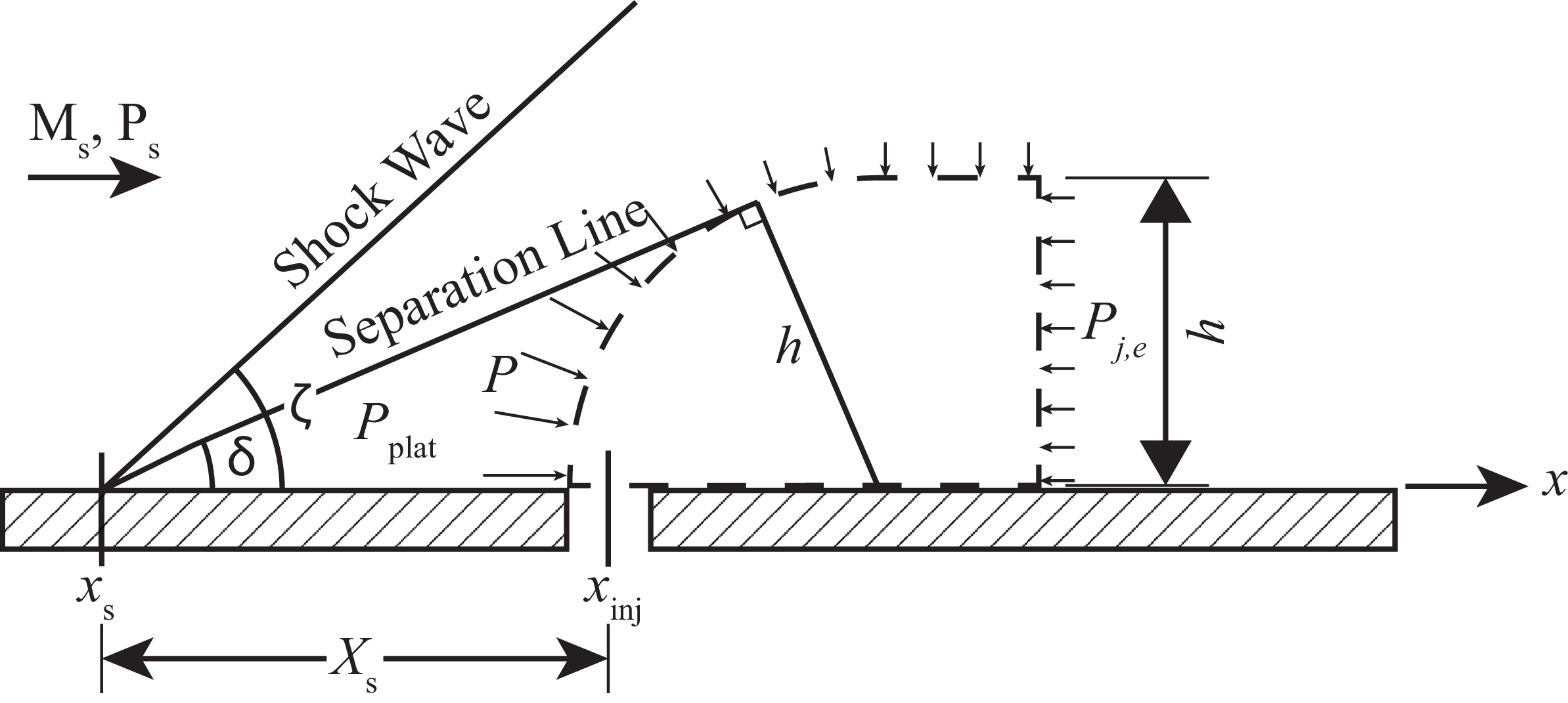
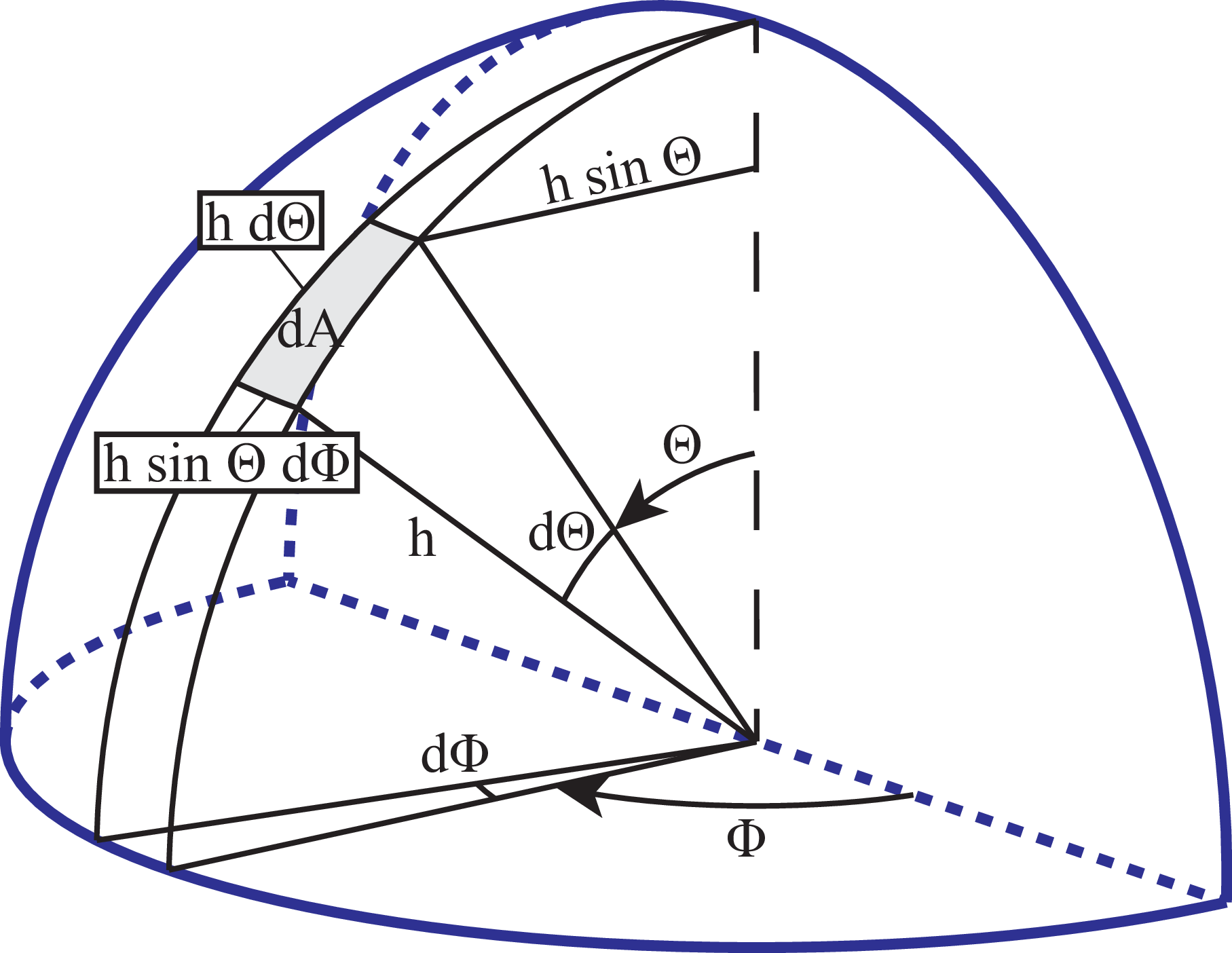
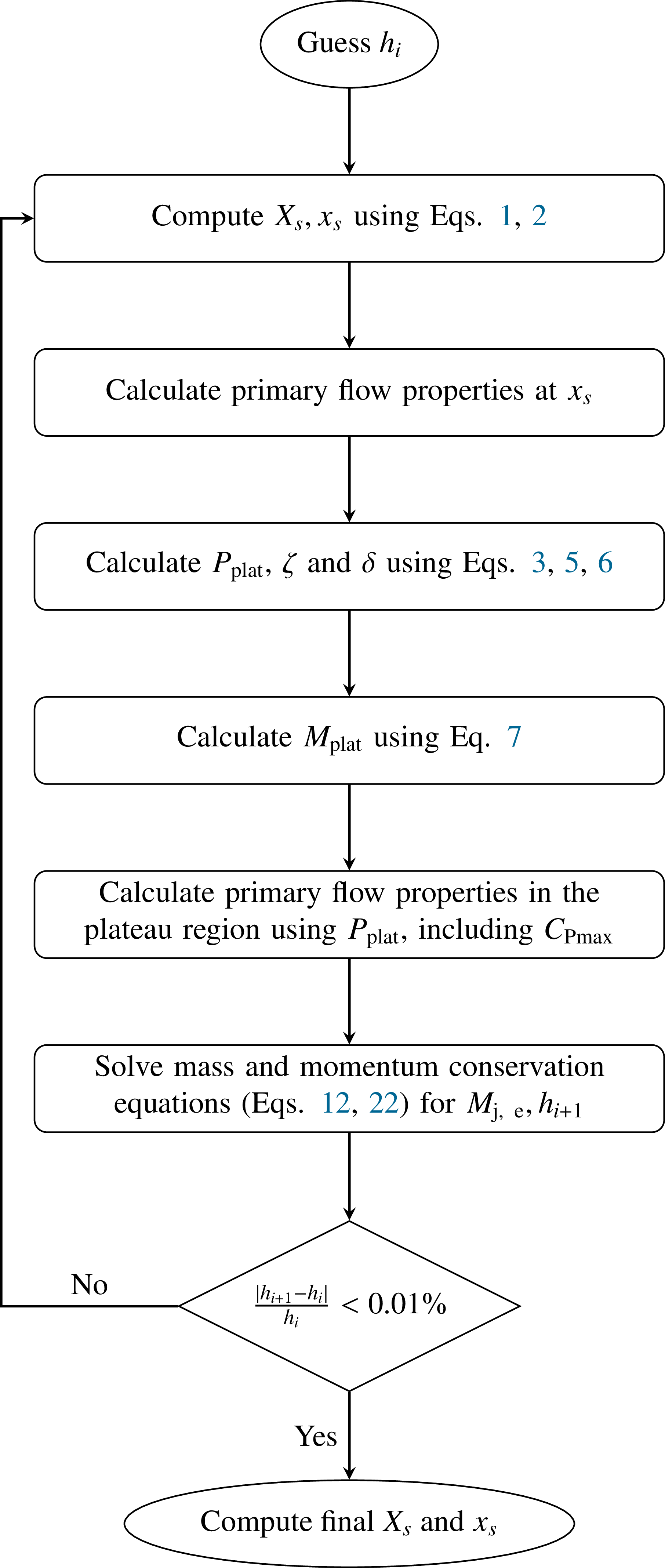
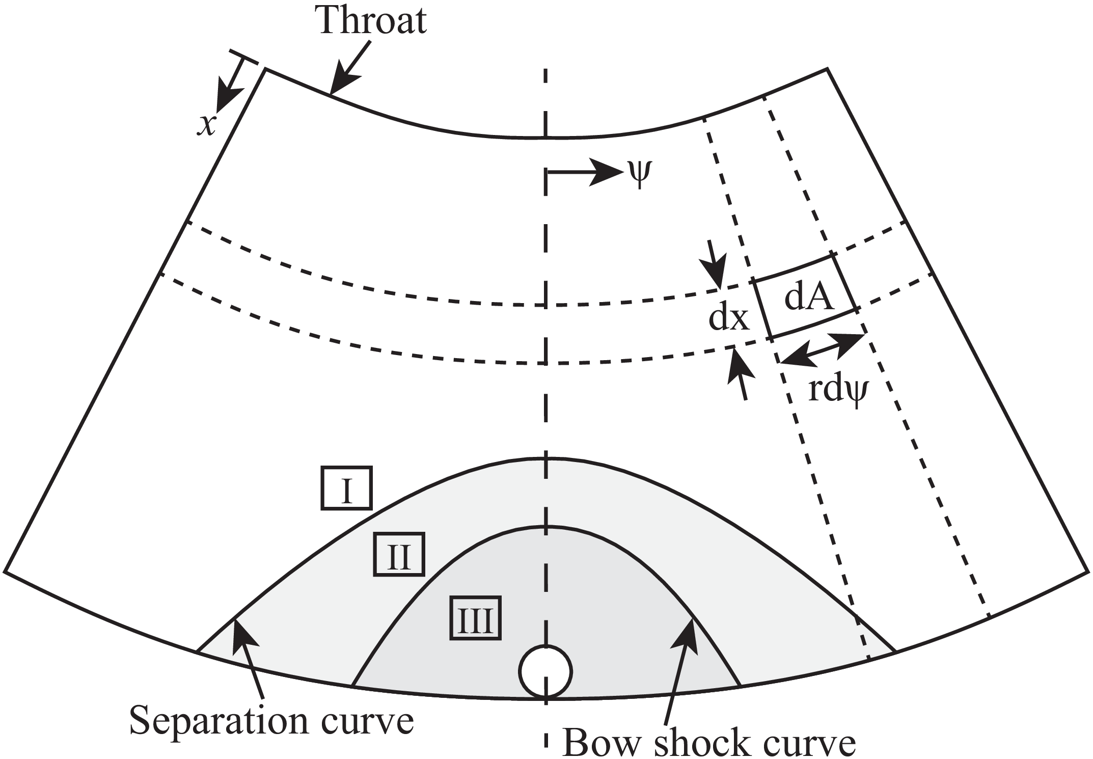
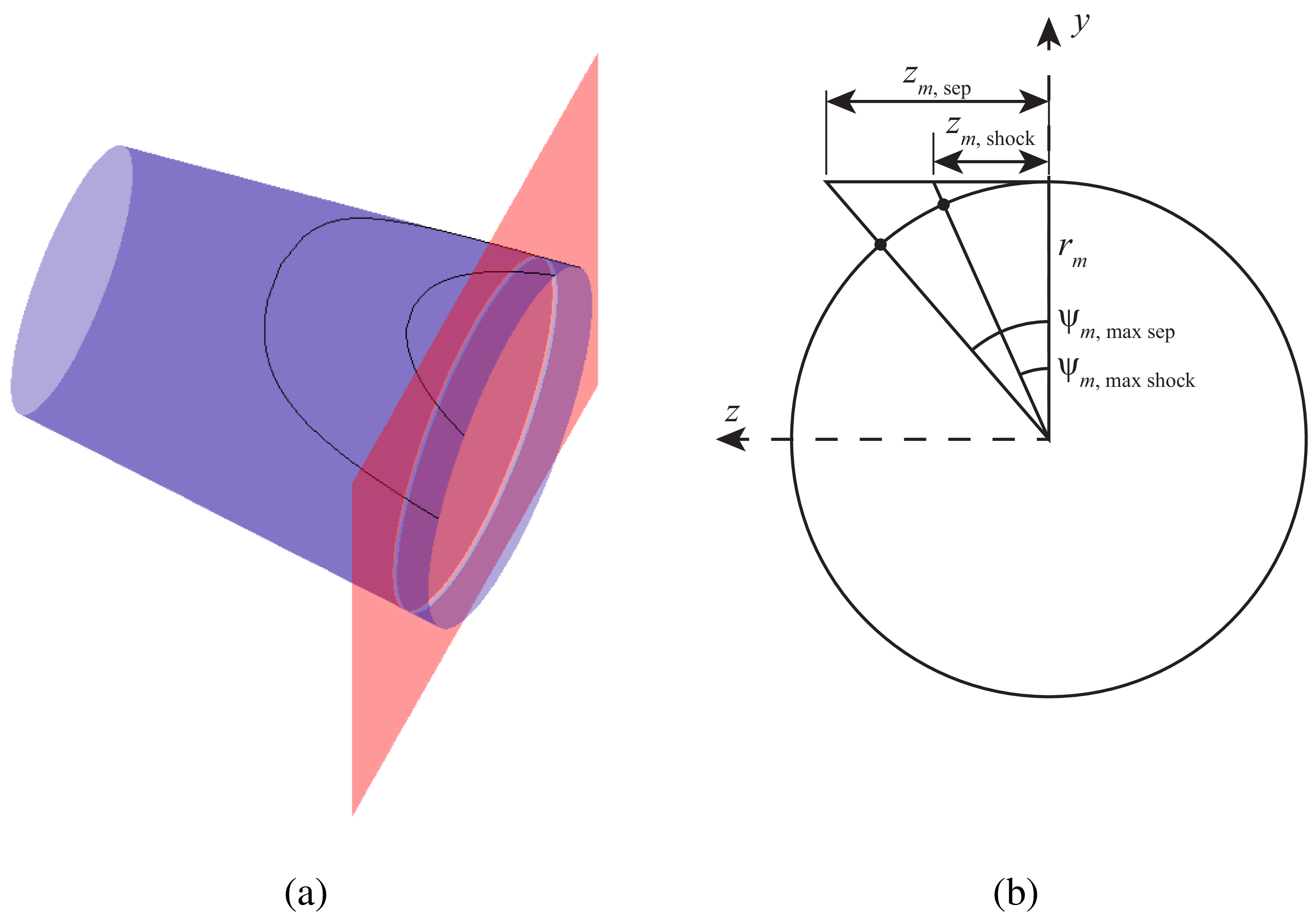
 ψm,max
 m
m
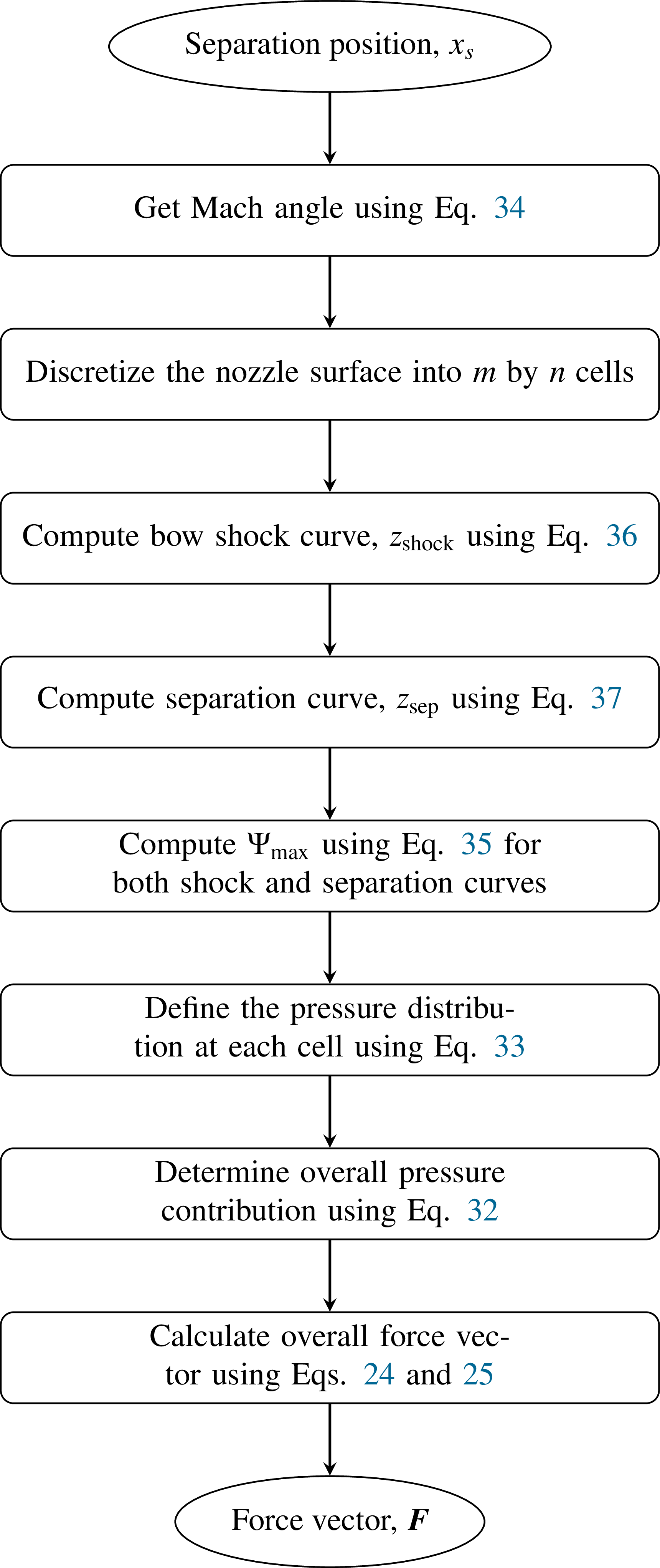
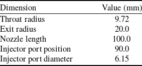


 x
x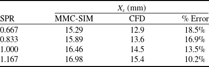
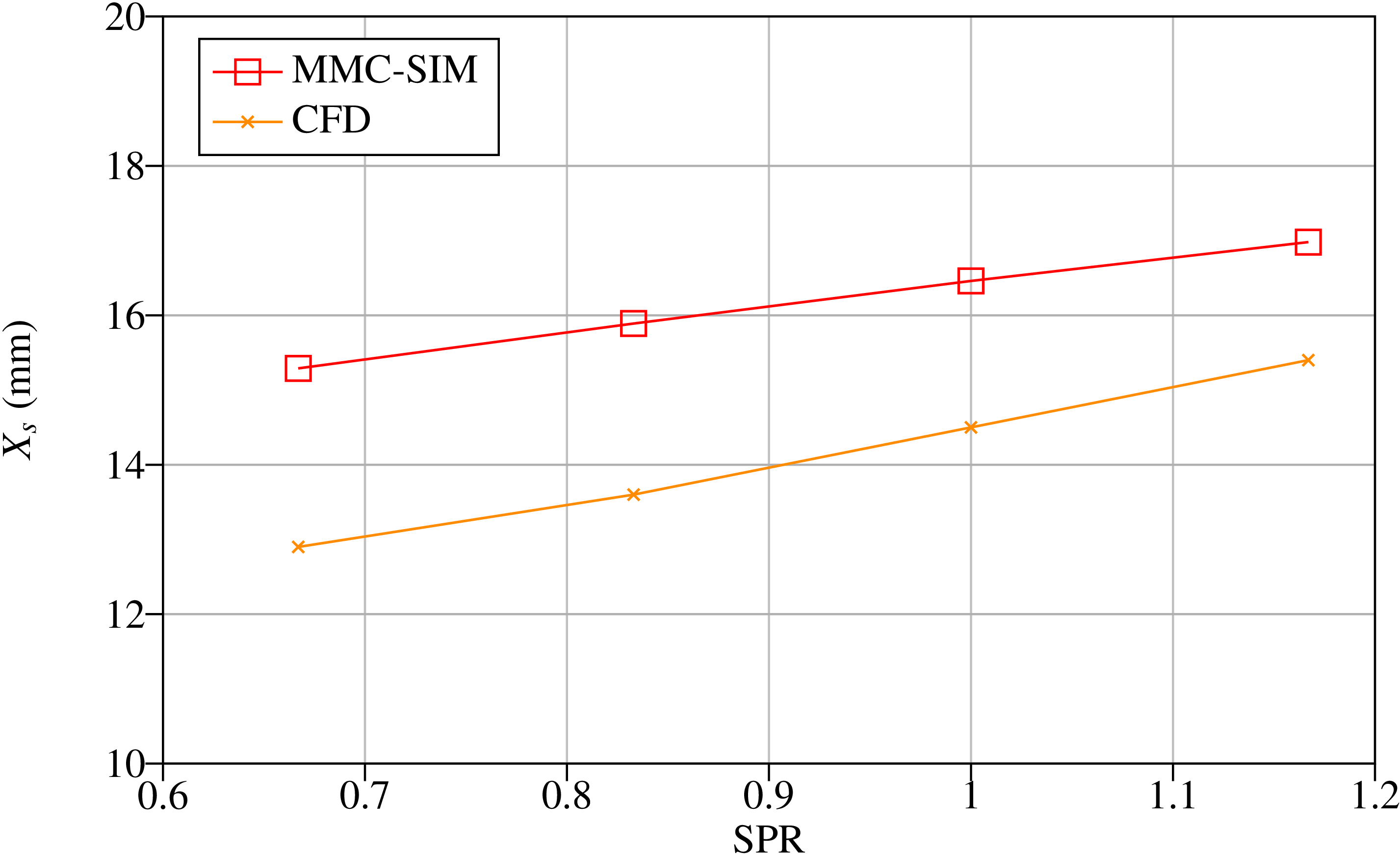

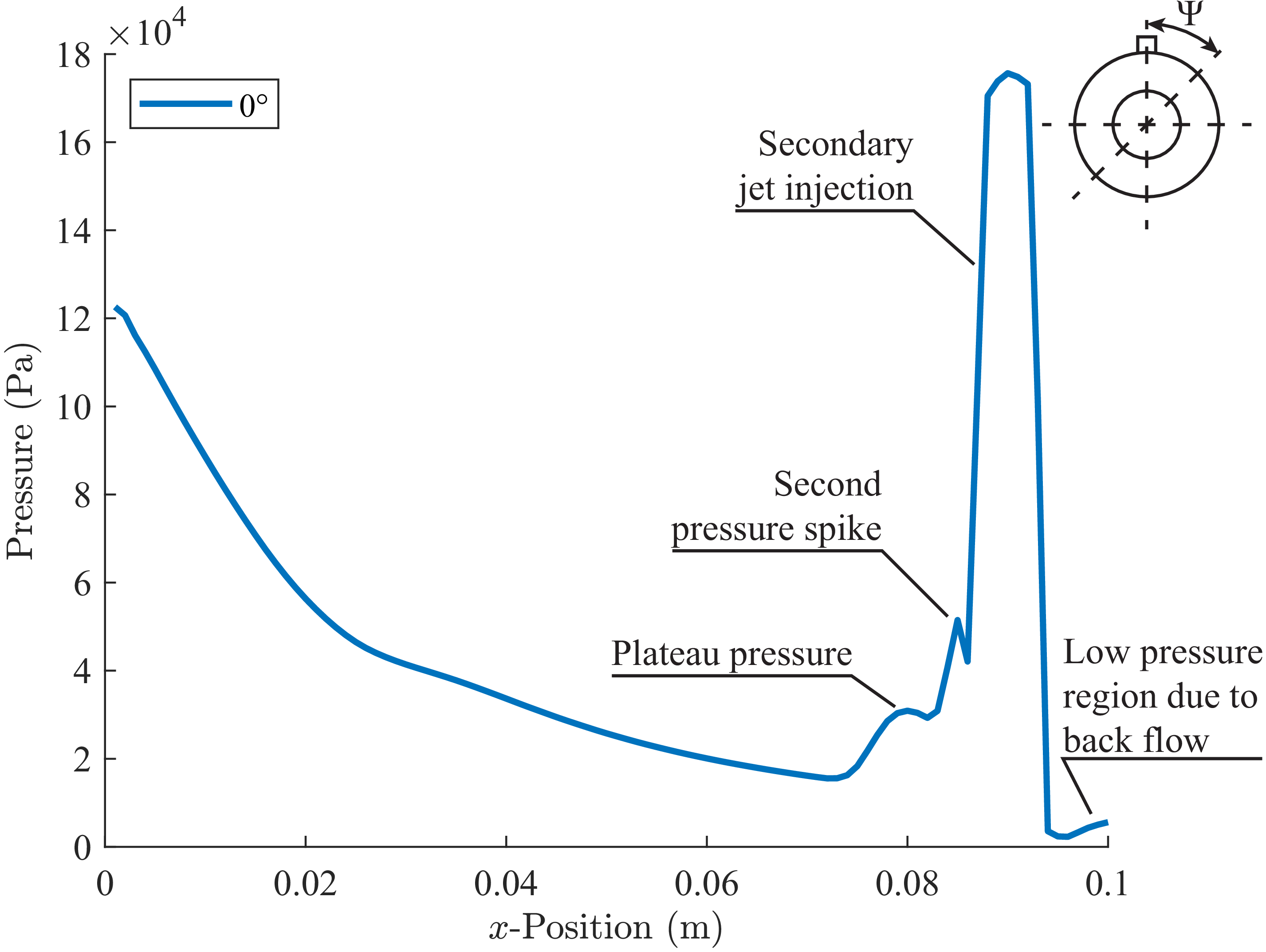
 Ψ=0∘
Ψ=0∘
 Ψ
Ψ
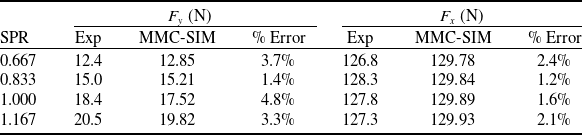
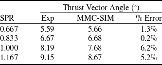
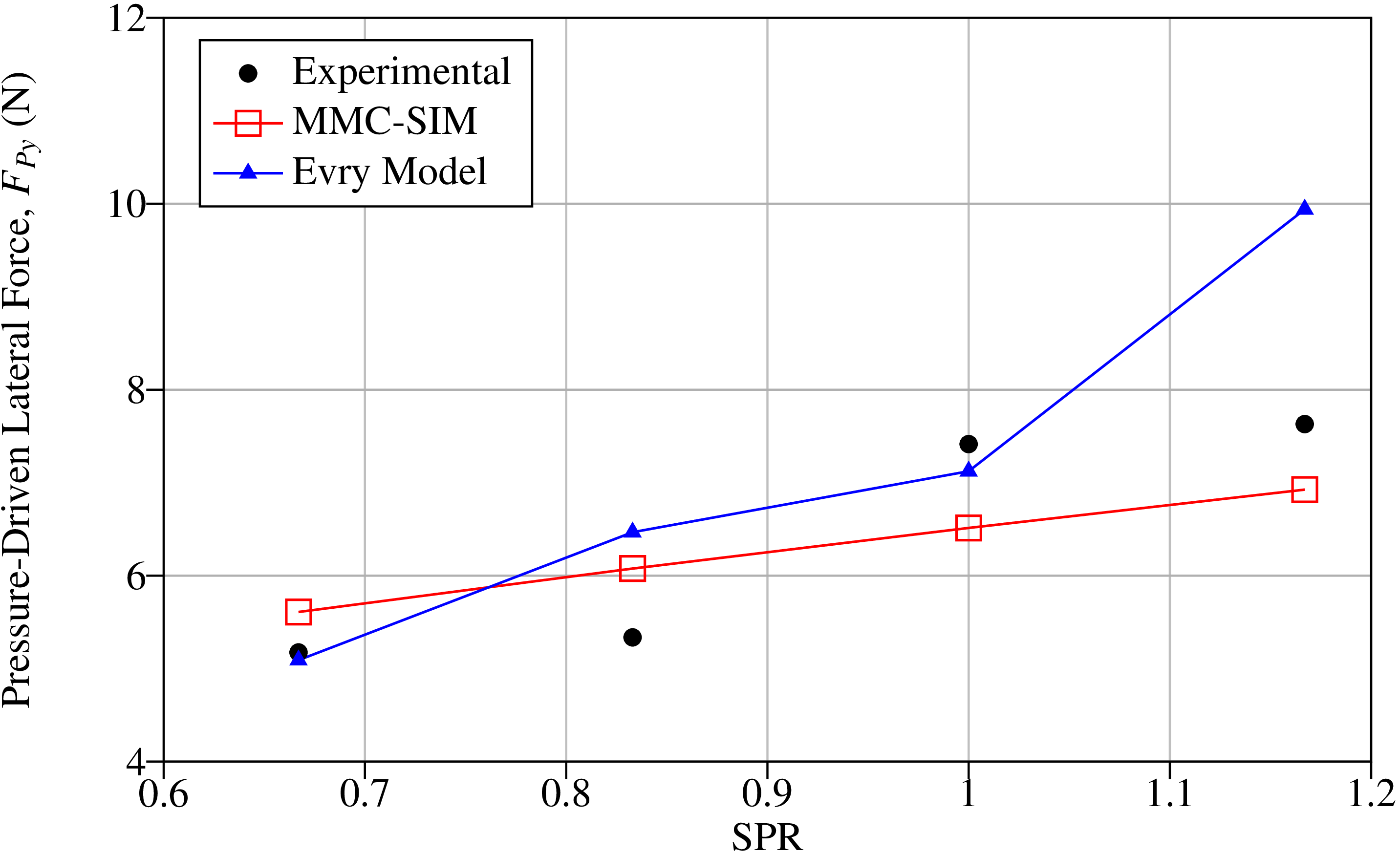
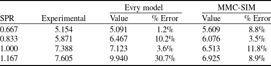


 Open access

