2.1. Study site

A terrestrial photographic survey was performed on a series of ice cliffs located in a partially drained lake basin on the Ngozumpa Glacier located in the upper Dudh Kosi catchment, Khumbu Himal, eastern Nepal (27°57′N, 85°42′E; Fig. 1a). The glacier flows southward from cirques below Cho Oyu (8188 m a.s.l.) and Gyachung Kang (7922 m a.s.l), where most accumulation occurs by ice and snow avalanching. The glacier is 18 km long and terminates at ~4660 m a.s.l.. The lower 15 km of the glacier is debris-covered and the last ~6.5 km of the glacier tongue is stagnant (Quincey and others, Reference Quincey, Luckman and Benn2009). The hummocky surface relief of the debris-covered glacier tongue is in the order of 30–50 m (Thompson and others 2016) and is studded with supraglacial ponds and associated exposed ice cliffs. The terrain of this glacier, its wasting processes and the evolution of supraglacial ponds have been relatively well studied (Benn and others, Reference Benn, Wiseman, Warren, Nakawo, Raymond and Fountain2000, Reference Benn, Wiseman and Hands2001; Thompson and others, Reference Thompson, Benn, Dennis and Luckman2012, Reference Thompson, Benn, Mertes and Luckman2016), as have the supraglacial debris properties, including limited measurements of debris thickness (Nicholson and Benn, Reference Nicholson and Benn2012). The lake basin is overlooked by upper-outer, and a lower-inner, lateral moraines allowing two separate vantage points to be used for taking photographs. A 1 m resolution DSM derived from Pléiades satellite imagery taken on the 12 April 2016 indicates that the inner and outer moraine ridges overlook the base level of the partially drained lake basin by ~78 and ~108 m respectively, and that the sampled ice cliffs rise up to 52 m above the base level of the partially drained lake basin (Fig. 1b).

Fig. 1.

(a) Pléiades imagery from 12 April 2016 showing the location of the Ngozumpa glacier (inset) and the study site (red box). (b) Map of the partially drained lake basin that forms the study site showing locations of the ice cliffs numbered 1–3 that were covered by the digital surface model, and the locations of available manual measurements of exposed debris thickness (Manual) at ice cliffs 1 and 2 and ground penetrating radar measurements of debris thickness (GPR lines) behind ice cliff 2.

2.2. Cameras and photography

We used a pair of 12.3 megapixel Nikon D5000 cameras with Tamron 70–300 mm macro lenses, set at a fixed focal length of 100 mm and ISO 200. This combination allows ground sampling distance (GSD) resolution of ~0.03 m per pixel at a distance of 0.5 km, which is about the furthest distance of ice cliff 2 (Fig. 1b). Both cameras were used to simultaneously capture images from the upper-outer and lower-inner lateral moraine crests (Fig. 1b). The survey was undertaken between 10:00 and 12:30 on 4 April 2016, in clear sky conditions. Over 2000 high-resolution JPEG images were taken to ensure a useful sub-sample would be available for deriving the model.

2.3. Ground control points (GCPs)

To provide GCPs for accurately scaling the surface model, seven 1 m² bright cloth targets were positioned on the glacier surface, and the central points of these were surveyed using a differential GPS system that comprised a Trimble XH6000 with Tornado antenna as rover and a Trimble Geo7X with Zephyr antenna as a local base station (Fig. 1b). The positions of the cloth targets (GCP Markers in Fig. 1b) were used to accurately georeference the surface model and an additional five prominent boulder locations (GCP Crosscheck in Fig. 1b) were surveyed as an independent means of evaluating the quality of the surface model. Point GPS data were collected at 1 s intervals and 3000 points were collected at each GCP location; these were differentially corrected, clear outliers were removed and the mean and standard deviation of the remaining points was used as the position and accuracy of the GCP. The maximum mean radial spherical error for the GCPs was 0.014 m, and maximum 99% spherical accuracy standard was 0.025 m.

2.4. SfM-MVS processing

Initial inspection of imagery was done to remove poorly focused images or those not covering the main ice cliff areas. Afterwards, 1160 full resolution JPEG images were imported unmodified into the Agisoft Photoscan (v1.26) software package for performing Structure from Motion with Multi-View Stereo (SfM-MVS) 3-D modelling. Considering the two sets of images were taken from two different cameras (albeit the same make, model and lens) they were separated for model generation into two specific camera groups. Initial alignment of images using the setting ‘Highest’ produced a sparse point cloud of 1 765 703 points. After removal of obvious erroneous points and those located in the far distance, the remaining points were filtered using the gradual filter settings. Points present in only one image pair, along with points having a reprojection error >0.5 pixels, were removed, leaving the sparse cloud with 341 150 points. This reprojection error threshold was chosen subjectively to balance minimizing the reprojection error with maximising the number of retained points. GCPs were next identified in all corresponding images and adjusted into position. The central point of the GCP targets was identified by picking the visible midpoint of the target. Based on the resolution of the images, we estimated a maximum placement accuracy of ~0.05 m at the furthest GCP markers. Model optimization was done using default parameters of f, b1, b2, cx, cy, k1-4, p1 and p2 and, as the lens distortion plot showed no extreme skewing or distortion, these optimization settings were accepted.

The dense point cloud was generated using the ‘High’ quality setting with ‘Aggressive’ point filtering. This took two days of processing time using an Intel i7-6700k 4 GHz processor with 8 MB cache and 64 GB RAM and a NVIDIA GeForce GTX980M graphics card, and resulted in a dense cloud of 150 822 811 points, with a mean point density of 478 points m⁻². As the photographic survey focussed on the ice cliff areas, point density per unit horizontal area around the cliffs is much higher (Fig. 2), although manual analysis of oblique 1 m⁻² samples of the debris exposures of interest indicates true local surface point density of 700–900 points m⁻². The dense point cloud was then used directly to generate the DSM and orthomosaic at resolutions of 0.046 and 0.023 m, respectively. The DSM resolution was determined on the mean point density over the whole model rather than the higher point density at the ice cliff areas. This represents a downgrade of the potential model resolution at the ice cliffs but was chosen as our locally high point densities are unlikely to be matched by those of photographic DSMs of larger glacier areas. These were then exported to TIFF format for further use in a GIS environment. The dense point cloud, DSM and orthophoto are available online (https://doi.org/10.5281/zenodo.883104).

Fig. 2.

Point density map of SfM-MVS point cloud used to generate the DSM.

2.5. Determining debris thickness from the SfM-MVS DSM

To determine the debris thickness (h _d) from the SfM-MVS DSM, the crest line of the debris and the visible boundary of the debris/ice interface below the ice cliff crestline were digitized manually in the 3-D Photoscan environment using a tiled model at full resolution and the polyline tool. Automatic methods of delineating the crest line and debris/ice interface were not attempted. The crest line can be problematic to identify in a DSM derived from terrestrial photographs where it coincides with the very edge of the surface facing the camera viewpoint, and a manual check of the DSM is required to ensure that the crest line picked is conclusively the debris crest. As surface properties and geometry of ice faces are observed to vary with aspect and season, automatic identification of the debris/ice interface is expected to be challenging. Surface classification schemes based on object-based training (e.g. Kraaijenbrink and others, Reference Kraaijenbrink, Shea, Pellicciotti, De Jong and Immerzeel2016) or decision-tree algorithms (e.g. Racoviteanu and others, Reference Racoviteanu and Williams2012) could be applied for a glacier-wide photographic survey, although it should be noted that a universal classification scheme might remain elusive. At the lateral margins of the ice cliffs, slumping of debris from above makes it difficult to confidently mark the interface, and here we present only data from unambiguously identified sections of the crest and interface lines.

The two sets of crest and debris/ice interface lines were imported to ArcMap (v10.4) where points were created every 1 m along the upper crest line, totalling 974 sample locations. The 3-D geometry of the exposed debris thickness is complex, and therefore we present two methods by which a point on the lower interface line corresponding to each crest line point can be identified. Firstly, we applied the ‘Steepest Path’ tool from the ArcMap Hydrology toolbox to provide an illustrative guide for manually picking a point pair location on the debris/ice interface beneath the crest line point. Secondly, we applied the ‘Nearest’ tool in the Proximity toolbox to find the minimum horizontal distance from each sampled crest line point to the debris/ice interface line, which offers an automatic method of defining a paired point for each crest line sample point. Hereafter these two methods of picking the paired debris/ice interface points are referred to as ‘Steepest’ and ‘Nearest’.

Figure 3 shows a schematic of the simplified geometry used to calculate debris thickness from each point pair consisting of a crest line point (C) and a debris/ice interface point (I). The exposed debris face is always sub-vertical, and the length of the exposed debris slope between each point pair can be directly measured from the DSM, or presented in a simplified linearized form as the length of the 3-D vector between the two points. However, determining the vertical thickness of debris at each crest point requires an assumption of the underlying ice surface extending back from the debris/ice interface to be made. In the absence of extensive geophysical measurements or excavation, the nature of this underlying ice surface is essentially unknowable. Accordingly, we proceed by initially making the assumption that the ice surface extends horizontally back from the debris/ice interface so that the vertical difference between each pair of points can be taken to indicate the debris thickness (h _d). The slope angle (θ°) of the linearized fall line (f), between the points, is obtained from simple trigonometry for a right-angled triangle (Fig. 3). In reality, there may be extremes of ice surface relief just behind the ice cliff face, for example, deep, debris-filled crevasses, where the ice cliff is spalling off, or very thin debris cover at a collapsing debris cover of an expanding ice face. Therefore, the uncertainty of the assumption of an underlying horizontal ice surface geometry is difficult to quantify. To generate a reasonable estimate of the likely error introduced by this assumption, we consider that the height change per unit distance along the exposed debris/ice interface can be used as a proxy for the scale of likely ice surface height change perpendicular to the ice cliff. We use the mean and standard deviation of the point-to-point slope along the exposed debris-ice boundary to bracket the uncertainty of the h _d value calculated assuming a horizontal ice surface underlying the debris exposure.

Fig. 3.

Schematic illustrating the linearized geometry of a fall-line (f ) with slope θ° between a crest line (C) and debris/ice interface (I) point pair. Assuming that the underlying ice surface extends horizontally beneath the debris exposure over the horizontal distance between the point pair (d), the debris thickness (h _d) is given simply as the vertical difference between the point pair. The error on h _d can be estimated for a range of likely ice surface angles (examples for 5° and 35° inclined ice surfaces are shown). The error associated with any assumed ice surface slope angle scales with d, which typically varies with h _d. Manual measurements of debris thickness record the approximate length of the fall line (f ).

2.6. Additional data on debris thickness

Two additional sources of debris thickness data are available for our study area, and these can be used to provide a degree of independent validation of the debris thicknesses derived from the scaled photographic model.

Firstly, debris thickness above part of the main ice cliff line was measured manually along the inclined exposed debris slope using a tape measure lowered from the ice cliff top at 49 locations at ~3 m intervals, where the debris crest appeared sufficiently stable to do this safely (Fig. 1b). The manual measurements were taken along the inclined exposure of the debris face, for which the slope angle at each measurement point was not recorded. The precise location of each measurement point was also not recorded, although the start and end points of the sampled ice cliff sections were marked with a handheld GPS with a stated accuracy of ±5–8 m. It is difficult to provide an accurate error assessment on these measurements, but we consider ± 0.05 m to be a reasonable estimate. We compared these manual measurements with the linearized fall line (f) over the sections of ice cliffs two and three, for which both data sources are available (Fig. 1b).

Secondly, a combined 200/600 MHz IDS GPR was used to survey short sections of the glacier surface ~10 m behind the ice cliff crest lines (Fig. 1b). Data were collected to a Lenovo Thinkpad using the IDS K2 FastWave software (v2.0). GPS measurements from a low precision device integrated with the IDS system allow the GPS time to be associated with each GPR trace. These low precision values were replaced with more accurate differential GPS coordinates collected using a Trimble XH and Tornado antenna mounted on top of the IDS GPR and a Trimble Geo7X and Zephyr antenna installed on the lateral moraine as a local base station. This set up allows the positional accuracy of <5 cm for the majority of points used. Where differential correction was not possible due to the satellite constellation, the low precision GPS positions were used for each GPR trace.

The appropriate signal velocity for the supraglacial debris was obtained by burying a 1.5 m long steel bar to a known depth and then passing the GPR over the buried target. This was carried out with both radar frequencies in both fine and coarse debris material. At the first site, the reflector from the iron bar was only identifiable in the 200 MHz profile, while at the second the reflector was visible in both the 200 and 600 MHz radargrams. As the signal velocities were similar in all cases, these were averaged to obtain a bulk value that is considered representative for all the radar lines measured. This bulk value is 0.157 m ns⁻¹, which is quite high, but not unreasonable in the light of other data (McCarthy and others, Reference McCarthy, Pritchard, Willis and King2017).

GPR data were processed using ReflexW software (v8.5), following recommendations from Jol and Bristow (Reference Jol and Bristow2003) and based on experience from the Lirung Glacier (McCarthy and others, Reference McCarthy, Pritchard, Willis and King2017). The traces were trimmed and combined, then plateau declipping and DC filter were applied, before using the autopick function to identify the groundwave onsets, which were then shifted to time zero. Subsequently, dewow, background removal, and band-pass filters were applied sequentially, and the debris/ice interface was picked using the autopick function and a visual check of its performance. We compared the debris thickness derived from the GPR with the debris thickness (h _d) obtained from the SfM-MVS DSM for sub-sections of ice cliff 2, for which GPR data are available (Fig. 1b).

3.1. Digital surface model

Total surface coverage of the DSM is limited by the oblique nature of the imagery. For example, the model shows unresolvable areas behind hummocks and ice cliff faces where imagery is sparse or the surface is not visible from the camera viewpoint. Yet, for favourably orientated ice cliffs coverage is good, with locally high point densities for mapping of the debris/ice interface and the upper debris crest line (Fig. 3). The DSM error calculated by Photoscan after optimization and bundle adjustment is given as 0.03 m, and appears evenly distributed over the surface. This error is comparable with the pixel resolution of the images at ice cliff 2, which is the most distant surveyed (Figs 1b, 4). Comparison of the scaled DSM with the five GPS check points, which have mean standard deviations of 0.004, 0.003 and 0.007 m in X, Y and Z respectively, shows a mean error of −0.07 ± 0.05 m.

Fig. 4.

Overview of the digital surface model produced from the SfM-MVS workflow showing the debris thickness (h _d) calculated using the Nearest method and assuming horizontal ice surface underlying the debris exposure. As in Fig. 1, camera positions are indicated in blue, GCPs for scaling the model are shown in red and GCPs used as a cross check on the model are shown in yellow. As an indicative scale the maximum heights of all three ice cliffs sampled here are ~50 m measured from the level of the supraglacial ponds in front of the cliff to the crest of the debris exposed above the ice cliff.

3.2. Debris thickness from the SfM-MVS DSM

For the three ice cliffs surveyed, the mean slope between successive points sampled along the debris/ice interface by the Steepest method was 22°, 17° and 20°. Averaging these provides an indicative ice surface undulation of 20° with a standard deviation of 15°. Therefore we can consider likely error associated with the debris thickness calculated using the assumption of a horizontal surface to be h _d ± ε _20°, and the likely minimum and maximum impacts of the underlying ice surface to be bracketed by calculating the debris thickness if the ice surface was sloping by ±5° and ±35° behind the exposed ice cliff (Fig. 3).

For the 974 sampled debris thicknesses derived from the photographic model using the Steepest (Nearest) method using an assumption of horizontally continuous ice surface behind the debris exposure, mean debris thickness with error associated with a 20° underlying ice slope is 2.08 ± 0.69 m (1.81 ± 0.63 m), with standard deviation of 1.69 m (1.48 m) and interquartile range spanning 0.80–2.85 m (0.73–2.42 m). This wide range of debris thicknesses is in agreement with observations of strong local variability in supraglacial debris thickness on other debris-covered glaciers (e.g. Mihalcea and others, Reference Mihalcea, Mayer and Diolaiuti2008; Zhang and others, Reference Zhang, Fujita, Liu, Liu and Nuimura2011; Zhang and others, Reference Zhang, Hirabayashi, Fujita, Liu and Liu2016; McCarthy and others, Reference McCarthy, Pritchard, Willis and King2017). The local distribution of debris thickness derived using either method is negatively skewed (Fig. 5a), in agreement with findings at this location from theodolite surveys in 2001 (Nicholson, Reference Nicholson2005, data not shown). The debris thickness is not correlated to the crest line elevation, indicating that no clear relationship exists between the terrain elevation and the debris thickness at this site. Some topographic highs, such as at ice cliff 1, support thicker debris cover, in agreement with the idea that differential surface ablation, caused by spatial variation in debris cover thickness, can form the hummocky relief observed on debris-covered glaciers. However, topographic highs at ice cliff 2 are not all characterized by thicker debris. Inherited ice surface topography or internal collapse of englacial voids, instead of differential ablation, could be important in determining the surface relief at the study site. Alternatively, the apparent lack of relationship between topography and debris thickness could be because processes of gravitational reworking and slow topographic inversion of the surface relief means that a debris thickness sample at any given point in time represents only a snapshot of the co-evolving debris thickness and surface relief. In either case, our data suggest that surface elevation cannot be used in a straightforward manner as a proxy for the debris thickness.

Fig. 5.

(a) Percentage frequency distribution (0.25 m bins) of debris thickness (h _d) calculated from 974 point pairs identified from the SfM-MVS DSM using the Steepest, and Nearest method using assuming a horizontal underlying ice surface. The interquartile ranges of each method are shown. (b) Scatterplot comparison of h _d derived using point pairs picked by Steepest and Nearest methods showing line of least squares and the correlation coefficient between the two sets of measurements. (c) Point by point comparison of h _d derived from the Steepest (showing error bars associated with an underlying ice slope of ±20° shown in grey) and Nearest (error bounds not shown for clarity) methods of picking point pairs. The vertical dotted lines denote the separate cliff sections sampled (see Figs 1 and 4).

At least at the lake basin studied here, the automatic method of picking point pairs using the automatic Nearest tool performs reasonably well, though with a slight negative bias compared with the manual point pair picking method (Table 1; Fig. 5). A point-by-point comparison of the methods (Figs 5b, c) illustrates that the differences between the Steepest and Nearest methods of picking point pairs is often, but not always, larger where debris is thicker as the combined complex geometry of the debris crest and ice interface make it difficult to predict the relationship between these two methods at any given point. Nevertheless, it seems a valuable approach to consider if applying the method to a wider glacier area.

Table 1.

Descriptive statistics for the debris thicknesses derived from the SfM-MVS DSM generated in this study, using either the Steepest or Nearest method of determining point pairs, and assuming the debris/ice interface to be horizontal (bold).

Alternative h _d values were also computed assuming the underlying slope surface is inclined by ±20 (extremes of ±5 and 35° in grey shading) representing the most likely (minimum and maximum) ice surface slope beneath the debris, excluding cases where the assumed slope of the underlying ice resulted in negative h _d values.

The absolute error associated with the unknown underlying ice surface increases with debris thickness (Fig. 5c). To bracket the maximum impact of the assumption of the horizontal ice surface, we calculate the debris thickness statistics for a range of underlying ice surface slopes (Table 1). If all other geometrical parameters are the same, the steeper the slope of the linearized fall line (θ°), the more reasonable it is to make the assumption of the horizontal extrapolation of the ice surface, as the distance (d in Fig. 3), over which this extrapolation is being made, is smaller. Mean slope angle of the linearized debris exposure (θ°) was 50.3° and 48.7° for the Steepest and Nearest methods respectively, indicating that the automatic Nearest method does not always capture the steepest fall line, even though the method captures the broad characteristics of the debris thickness distribution reasonably well. In >90% of the cases for both methods, the slope of the debris exposures at these west-facing ice cliffs is higher than the angle of repose for coarse angular talus (~35°; Carson, Reference Carson1977), indicating a degree of cementing or consolidation within the matrix-supported diamict comprising the supraglacial debris (Nicholson and Benn, Reference Nicholson and Benn2012).

3.3. Comparison of SfM-MVS derived debris thickness with alternative debris thickness data

The h _d values derived from measurements from the SfM-MVS DSM are not directly comparable with those determined by manual measurements or using GPR, as the exact measurement locations do not coincide. Therefore, due to the expected high degree of spatial variation in debris thickness, perfect correspondence between the datasets cannot be expected. Nevertheless, we compare sub-samples of the debris thickness determined using the Steepest method, and assuming a horizontal ice surface, over sections of the ice cliff nearest to the manual and GPR measurements. The debris thicknesses from the photographic DSM are broadly in keeping with those available from alternative measurement methods at this site (Table 1; Fig. 6), although Mann–Whitney U tests reject the hypothesis that they are samples from the same population. The f distribution derived from the SfM-MVS is positively biased compared with, and not as negatively skewed as, the manual measurements of f. This may be in part due to the fact that we have only approximate locations for the manual measurement so the subset of the SfM-MVS f values may not sample different sections of debris exposure, and as the sample size is small this could have a large impact on the comparison. The SfM-MVS h _d values closest to the available GPR measurements are an unusual subset of the data in that they show a relatively normal distribution and a substantially lower mean debris thickness compared with the whole dataset (Tables 1 and 2). There is no evidence that the debris surface behind the debris crestline was being modified by slumping as would be the case if gravitational reworking was reducing debris thickness beneath the crestline and, thus, the local comparison between these datasets, therefore, indicates thickening of debris behind the ice cliff line around ice cliff 2, such that the ice surface underlying the debris exposure must dip away from the exposed face. This means that debris thicknesses calculated assuming a horizontal ice surface underestimate the true debris thickness beneath the crest line at this section of the ice cliff. Although the local comparison between the SfM-MVS and the GPR debris thickness appears poor, the whole dataset of SfM-MVS debris thickness compares very well with the GPR data (see Tables 1 and 2; Figs 5a, 6b). This agreement gives added confidence to the ideas that a single electromagnetic velocity for the GPR analysis is acceptable, and that the SfM-MVS technique is capturing similar debris thickness distribution to that found behind the ice cliffs.

Fig. 6.

Percentage frequency (0.25 m bins) of debris thicknesses (h _d) comparisons between (a) SfM-MVS DSM and manual fall line distance (f ) and (b) SfM-MVS h _d at the debris exposure and GPR h _d measured ~10 m behind the cliff crest line.

Table 2.

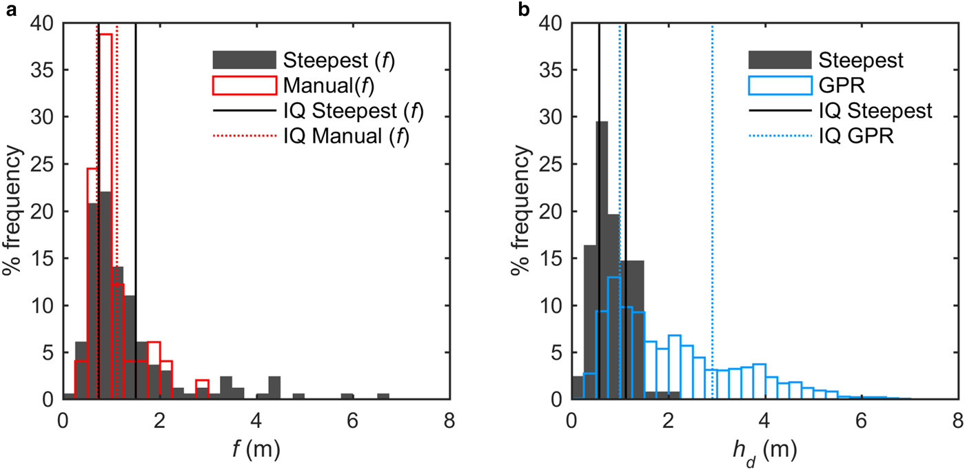
Descriptive statistics for the debris thicknesses metrics derived from the SfM-MVS DSM using the Steepest method of determining point pairs, applied to subsets of the available data most closely located to the manual (f) and GPR (h _d) measurements available

Our data indicate mean debris thicknesses in this area are in the region of 2.0 m, which is much thicker than the daily temperature wave penetration depth observed from measured temperature profiles (Nicholson and Benn, Reference Nicholson and Benn2012). This may partly explain why the h _d range we derive from the SfM-MVS DSM overestimates values determined in other studies using ASTER surface temperatures and a simplified energy-balance model (e.g. Rounce and others, Reference Rounce and McKinney2014), which indicate debris thickness of ~0.1–0.4 m at the study site. A second contributing factor is likely to be the widespread distribution of supraglacial ponds and exposed ice cliffs in and around the study site, which means that each ASTER pixel will include the surface temperature of ponds and exposed ice. Combining local debris thickness distribution data obtained from photographic surveys with estimates from satellite imagery offers a means of deriving more accurate debris thickness distributions from the satellite imagery.

3.4. Evaluation of the utility of SfM-MVS DSMs for determining supraglacial debris thickness

Our findings indicate that photographically-derived DSMs can offer a relatively cost-effective, quick and straightforward means of estimating debris thickness at exposed ice cliffs. The high resolution of the DSM derived here is related to the use of reasonably high specification cameras in combination with zoom lenses in order to obtain pixel resolutions sufficient to enable meaningful measurements at the range of the expected debris thickness. Lower resolution cameras, such as the lighter weight cameras often used with UAVs, would reduce the model quality. However, this limitation can be offset by taking images closer to the ice cliff lines of interest. The accuracy of the measurements possible is also affected by the quality of the GCPs, thus any DSM used for the analysis presented here requires sufficiently high quality, well-distributed GCPs to accurately scale the DSM.

The use of terrestrial photography as presented here introduces a sampling bias as only ice cliffs with favourable aspects for viewing from a lateral moraine or a similar vantage point can be sampled. This could be overcome by a wider photographic survey, or more practically, by use of an oblique-angled camera mounted on a UAV and flown along ice cliff edges. Regardless of vantage point biases, the extent to which the debris thickness exposed above ice cliffs is representative of debris thickness in the surroundings remains an open question. As ice face backwasting is governed by subaerial ablation, waterline undercutting and calving, which are independent of the overlying debris thickness (e.g. Reid and Brock, Reference Reid and Brock2014; Steiner and others, Reference Steiner2015; Brun and others, Reference Brun2016; Miles and others, Reference Miles2016), it seems reasonable to assume that at any point in time the debris exposed above ice cliffs offers a fairly random sample of the debris thickness of the region. The terrain sampled by our SfM-MVS DSM has a total relief of 65 m, compared with 34 m of relief covered by the sampled debris exposures. The ice cliffs at the study site do not cross-cut former supraglacial pond sediments, but further down-glacier ice cliffs around supraglacial ponds do. This indicates that within sufficiently mature debris cover, that has undergone some degree of topographic inversion due to differential ablation and gravitational redistribution of surface debris, exposures above ice cliffs can sample former topographic lows, even though they typically occupy higher terrain in the current topography.

Comparing the data generated from ice cliff line sampling with that from wider manual excavations and geophysical explorations in terrain that does not contain ice cliff exposures would be valuable for understanding the degree to which the ice cliffs represent a random sample of local debris thickness. Statistical analysis of debris thickness at sampled ice cliffs can be expected to suffer from spatial autocorrelation, but sampling a sufficiently wide area, including ice cliffs of all sizes and orientations, would minimize sampling bias. Many glaciers, including Ngozumpa, have ice cliffs occurring throughout almost the whole debris-covered area (e.g. Watson and others, Reference Watson, Quincey, Carrivick and Smith2017), permitting this sampling technique to be applied to examine the variation in debris thickness down the length of the glacier, either by building DSMs of the whole glacier tongue or several small sections forming a down-glacier transect.

The assumption used here that the debris/ice interface extends horizontally back from the exposed ice cliff beneath the debris is unlikely to be met, given the roughness of the glacier surface above and within the debris cover. However, the nature of the surface beneath the debris cover cannot be determined without the use of extensive geophysical surveys. As neither a visual inspection nor correlation analysis indicated a systematic relationship between terrain height and debris thickness along the sampled ice cliffs we elected to use the simpler assumption of horizontal continuity of the debris/ice interface and compute error bounds based on the characteristic surface slope of the underlying ice. A wider sampling area including many more ice cliffs may yet reveal a useful relationship between local topography and debris thickness that could be used to improve upon this simple assumption. As ablation at ice cliffs is rapid, in the case of Ngozumpa glacier accounting for 40% of volume losses over the lower part of the glacier tongue (Thompson and others, Reference Thompson, Benn, Mertes and Luckman2016), repeat analysis of high-resolution photographic DSMs over time, that have been used to monitor ice cliff backwasting (e.g. Brun and others, Reference Brun2016; Buri and others, Reference Buri2016), would also reveal the spatial distribution of debris thickness behind the ice cliffs in the form of a time-space substitution. More extensive measurements of the underlying ice surface and debris thickness using high frequency GPR (McCarthy and others, Reference McCarthy, Pritchard, Willis and King2017) offers a useful tool for determining relationships between surface terrain and underlying terrain that can be expected to offer valuable information in determining the validity of the assumption of horizontal extension of the debris/ice interface applied in this study.