


1. Introduction
Recent observations indicate that mass losses from the Greenland ice sheet have increased (Reference Rignot and KanagaratnamRignot and Kanagar-atnam, 2006; Reference Velicogna and WahrVelicogna and Wahr, 2006), with concomitant increases in global sea level (Reference Pritchard, Arthern, Vaughan and EdwardsPritchard and others, 2009; Reference Rignot, Velicogna, Van den Broeke, Monaghan and LenaertsRignot and others, 2011). One recent estimate puts the increase in mass loss from Greenland at 21.9 ± 1Gta-2 since 1992 (Reference Rignot, Velicogna, Van den Broeke, Monaghan and LenaertsRignot and others, 2011), despite slow thickening at higher elevations (Reference Pritchard, Arthern, Vaughan and EdwardsPritchard and others, 2009; Reference Thomas, Frederick, Krabill, Manizade and MartinThomas and others, 2009). Mass is lost by two broad processes: (1) surface melting and runoff, and (2) dynamic thinning and iceberg calving associated with accelerated ice flow. Contemporary mass losses are split approximately equally between the two processes (Reference HannaHanna and others, 2008; Reference Van den BroekeVan den Broeke and others, 2009).
Both processes are accelerating. Surface melting and runoff have increased over the last two decades (Reference Hanna, Huybrechts, Janssens, Cappelen, Steffen and StephensHanna and others, 2005; Reference MoteMote, 2007; Reference Mernild, Liston, Steffen, Van den Broeke and HasholtMernild and others, 2010) coincident with a global warming signal (Reference HannaHanna and others, 2008). During 1995-2007 the average freshwater flux to the ocean was ~786km3a-1 (Reference Mernild and HasholtMernild and others, 2009) compared to 1953-2003 rates of ~281km3a-1 (Reference Janssens and HuybrechtsJanssens and Huybrechts, 2000); high summer melt rates have further intensified since 2006 (Reference Van de WalVan den Broeke and others, 2008). Widespread dynamic thinning has been observed at latitudes south of 70° N (Reference Rignot and KanagaratnamRignot and Kana-garatnam, 2006) and more recently at all latitudes, penetrating up to 120 km into the ice-sheet interior (Reference Pritchard, Arthern, Vaughan and EdwardsPritchard and others, 2009). Many of the largest observed dynamic mass losses are associated with marine-terminating glaciers. Likely mechanisms include the warming of fjord waters associated with atmospheric forcing (Reference MurrayMurray and others, 2010; Reference ChristoffersenChristoffersen and others, 2011; Reference StraneoStraneo and others, 2011), and disintegration of buttressing floating ice tongues and sikkusak (ice melange) (Reference Thomas, Frederick, Krabill, Manizade and MartinThomas and others, 2009; Reference Howat, Box, Ahn, Herrington and McFaddenHowat and others, 2010). However, ice motion and dynamic thinning has also been observed to accelerate coincident with increases in meltwater inputs to the englacial and subglacial environment, predominantly in land-terminating regions (Reference Zwally, Abdalati, Herring, Larson, Saba and SteffenZwally and others, 2002; Bartho-Reference Bartholomaus, Anderson and Andersonlomaus and others, 2008; Reference Van de WalVan de Wal and others, 2008; Reference Shepherd, Hubbard, Nienow, McMillan and JoughinShepherd and others, 2009; Reference Bartholomew, Nienow, Mair, Hubbard, King and SoleBartholomew and others, 2010, 2011; Reference Palmer, Shepherd, Nienow and JoughinPalmer and others, 2011) but also at the marine-terminating Helheim Glacier, East Greenland (Reference AndersenAndersen and others, 2010), and Kangiata Nunata Sermia, southwest Greenland (Reference SoleSole and others, 2011). Consensus regarding the relative importance, spatial applicability and precise mechanisms associated with this effect remains to be established (Reference Joughin, Das, King, Smith, Howat and MoonJoughin and others, 2008; Reference LuthiLüthi, 2010).
A key uncertainty in both mass-balance estimates and our understanding of coupled hydrology/ice-motion mechanisms is therefore meltwater runoff. Not all meltwater produced at the surface exits the ice sheet: some is retained (e.g. in the interstitial pore structures of snow and firn) and therefore continues to contribute to the total ice mass (Reference FountainFountain, 1996; Reference Wadham and NuttallWadham and Nuttall, 2002; Reference Jansson, Hock and SchneiderJansson and others, 2003; Reference ParryParry and others, 2007). In the absence of runoff measurements, ice-sheet mass-balance estimates rely on parameterizations or models of surface meltwater retention and refreezing (Reference Pfeffer, Meier and IllangasekarePfeffer and others, 1991; Reference HockHock, 2005; Reference Van de WalVan den Broeke and others, 2008). Proglacial discharge gauging records commonly used in alpine studies as an indicator of surface-to-bed hydrological coupling exist for only a few locations in Greenland (e.g. Skeldal River, northeast Greenland (Reference Stott and GroveStott and Grove, 2001); Kanger-lussuaq, West Greenland (Reference Mernild and HasholtMernild and Hasholt, 2009); and Leverett Glacier, West Greenland (Reference BartholomewBartholomew and others, 2011)) and are often of short duration owing to the expense and logistical difficulties of extended field studies.
One possible alternative indicator of runoff from the ice sheet into the ocean is sediment plumes produced by glacial meltwater entering the sea. Fine sediments are produced by erosion of the glacier bed (Reference Hallet, Hunter and BogenHallet and others, 1996) and can be flushed out by subglacial water flow (Reference Hubbard and NienowHubbard and Nienow, 1997). Higher volumes of proglacial discharge tend to coincide with relatively higher suspended sediment concentrations (SSCs; Reference Fenn, Gurnell and ClarkFenn, 1987). Turbid meltwater emerging from the subglacial environment into coastal waters forms sediment plumes clearly identifiable in satellite imagery (Reference Lewis and SmithLewis and Smith, 2009). The application of multispectral remote sensing to mapping turbidity and sediment plume extent is well established (Reference Curran, Hansom, Plummer and PedleyCurran and others, 1987; Reference Stumpf, Gelfenbaum and PennockStumpf and others, 1993; Reference Ruhl, Schoellhamer, Stumpf and LindsayRuhl and others, 2001; Reference Miller and McKeeMiller and McKee, 2004).
Very little research has explored the feasibility of using sediment plumes as indicators of ice-sheet runoff onset, duration and variability. Recent studies in Søndre Strømfjord, West Greenland, concluded that satellite-based quantification of sediment plumes using Moderate Resolution Imaging Spectroradiometer (MODIS) imagery offers an inexpensive, widely applicable alternative to constraining runoff from individual catchments using gauging stations (Reference Chu, Smith, Rennermalm, Forster, Box and ReehChu and others, 2009; Reference McGrath, Steffen, Overeem, Mernild, Hasholt and Van den BroekeMcGrath and others, 2010), particularly if combined with observations of supraglacial melting, drainage and ice motion. The area and length of plumes in Søndre Strømfjord is linked with good confidence to (1) ice-sheet surface melt extent (Reference Chu, Smith, Rennermalm, Forster, Box and ReehChu and others, 2009) and (2) catchment precipitation and gauged runoff from the Watson River (Reference McGrath, Steffen, Overeem, Mernild, Hasholt and Van den BroekeMcGrath and others, 2010).
Winds may influence plumes over daily to seasonal timescales (Reference Stumpf, Gelfenbaum and PennockStumpf and others, 1993). Observations at lower latitudes indicate that when the wind blows down-fjord, a plume will narrow, while if the wind blows up-fjord, more rapid mixing of buoyant waters will occur (Reference Whitney and GarvineWhitney and Garvine, 2005). Winds in West Greenland often blow persistently up-fjord during the summer months (Reference Farmer and FreelandFarmer and Freeland, 1983), but are likely to be of less importance in sheltered environments than open bays. Reference McGrath, Steffen, Overeem, Mernild, Hasholt and Van den BroekeMcGrath and others (2010) find no relationship between wind speed and plume length in Søndre Strømfjord.
Tides principally modify the sub-diurnal evolution of freshwater plumes, as they can flush fjords during their ebb phase and retard plume evolution during their flood phase (Reference CowanCowan, 1992). Their modes of variability may be predicted using tidal harmonics and local gauging-station data, although the occurrence of complex internal tides related to fjord geometry can obfuscate these modes (Reference Tverberg, Cushman-Roisin and SvendsenTverberg and others, 1991). Greenland has micro to meso tidal ranges, so river flow is more likely to dominate. Reference Chu, Smith, Rennermalm, Forster, Box and ReehChu and others (2009) find no evidence to suggest that tides modify plume extent in Søndre Strømfjord.
This study seeks to assess the viability of using sediment plume areas as indicators of runoff from the ice sheet to the ocean at a number of outlets around the Greenland ice sheet. Meltwater catchment areas, proglacial terminus configurations and fjord geometries vary widely around Greenland. If the technique can be implemented for other outlets besides Søndre Strømfjord it may be able to enhance our ability to further constrain variability in ice-sheet mass loss and coupled hydrology/ice-motion dynamics.
Automated remote sensing is likely to be the only realistic method of observing runoff from many of the Greenland ice sheet's ~460 outlets (Reference Lewis and SmithLewis and Smith, 2009). This study therefore develops an automated sediment plume quantification system based on daily MODIS satellite imagery. The feasibility of automatically observing plumes at these locations is assessed in terms of technical accuracy and viability and the extent to which plumes capture the physical process of runoff.
2. Study Areas
Thirty-six outlets spanning the whole length of the West Greenland coast are chosen for examination. The selection encompasses the majority of land-terminating outlets visible at the 250 m spatial resolution of MODIS, apart from a few with short fjords likely to be strongly affected by regional winds or ocean currents. A number of marine-terminating outlets are also specified in order to investigate whether sediment plumes in these environments can be identified remotely. We primarily examine marine-terminating outlets with minimal proximal icebergs and sea-ice presence based on MODIS imagery from summer 2007. This restricts our selection to slower-moving marine-terminating glaciers, compared to glaciers such as Jakobshavn Isbræ which tend to produce large quantities of icebergs. Outlets are examined from 2000 to 2007 (in line with MODIS data availability) between 1 May and 30 September.
The outlets span a broad variety of coastal fjord and bay geometries which we classify as follows:
-
Land-terminating – proglacial river. Runoff from the ice- sheet margin collects into a distinct channel before reaching the fjord. In some fjords, rivers from multiple catchments reach the fjord within kilometres of each other. These are highlighted in our subsequent analysis.
-
Land-terminating – outwash plain. A proglacial braided channel system links the ice front to the the fjord.
-
Marine-terminating – calving (bay). The marine-terminating ice front either calves straight into a bay significantly wider than the ice front, or into a fjord which broadens out to a bay within ˜5 km. These outlets are therefore directly subject to coastal processes.
-
Marine-terminating – calving (fjord). The marine-terminating ice front calves across the whole width of a fjord, into a fjord >5 km long, and may be part of a longer and more sinuous fjord system. Marine and coastal influences are expected to be significantly less than in bay calving environments.
Outlets are identified based on the MODIS tile within which they reside, plus a number incrementing from north to south within each tile. For example, Søndre Strømfjord is H15V02:1. Not all outlets are retained for full analysis, due to insufficient temporal resolution. Figure 5 (further below) indicates the classifications of outlets retained after analysis, and their associated ice-sheet hydrologic subbasins identified from a hydrologic potential analysis (Reference Lewis and SmithLewis and Smith, 2009).
3. Data and Methods
3.1. Remote sensing of plumes
The spatial extent of buoyant freshwater sediment plumes may be defined as the area of water meeting a specified minimum SSC threshold. Field observations of SSC can be used to define the spectral signature of plumes in multi-spectral remotely sensed imagery, as for example undertaken in Søndre Strømfjord by Reference Chu, Smith, Rennermalm, Forster, Box and ReehChu and others (2009).
This study continues the remote-sensing methodology adopted by Reference Miller and McKeeMiller and McKee (2004), Reference Chu, Smith, Rennermalm, Forster, Box and ReehChu and others (2009) and Reference McGrath, Steffen, Overeem, Mernild, Hasholt and Van den BroekeMcGrath and others (2010) of using daily multispectral MODIS imagery acquired by the sun-synchronous, near-polar orbiting Terra satellite. MODIS acquires data in the visible portion of the spectrum over seven spectral bands at a spatial resolution of 500 m, and two bands at 250 m resolution. Here band 1 (846-871 nm) at 250m spatial resolution is employed, because glacially derived sediment plumes have already been identified and calibrated in this band by previous studies (Reference Chu, Smith, Rennermalm, Forster, Box and ReehChu and others, 2009; Reference McGrath, Steffen, Overeem, Mernild, Hasholt and Van den BroekeMcGrath and others, 2010). We use the MOD09GQ surface reflectance product, which has been corrected to provide an estimate of the surface spectral radiance at ground level if there were no atmospheric scattering or absorption. It is used in its native equal-area sinusoidal projection. MODIS products are rigorously quality-controlled. Comprehensive quality checks are carried out during processing to create end-user products of 'L2G' status, and extensive data-quality information accompanies the products (Reference Vermote, Kotchenova and RayVermote and others, 2011).
Spectral reflectance thresholds defining the presence of glacial sediment plumes in MODIS imagery are based upon those defined by Reference Chu, Smith, Rennermalm, Forster, Box and ReehChu and others (2009) and Reference McGrath, Steffen, Overeem, Mernild, Hasholt and Van den BroekeMcGrath and others (2010). The minimum threshold is 0.05, which corresponds to the minimum 'plume periphery' threshold set by Reference McGrath, Steffen, Overeem, Mernild, Hasholt and Van den BroekeMcGrath and others (2010). This is used in preference to the more stringent threshold of 0.12 used by Reference Chu, Smith, Rennermalm, Forster, Box and ReehChu and others (2009) because it increases the likelihood of automatically identifying a geometrically coherent plume. Plumes initially identified by this 'periphery' threshold are then tested against a 'plume core' threshold of 0.10. At least 10% of pixels composing the plume must have spectral reflectance values greater than this 'plume core' threshold. This reduces the propensity for false classification of essentially brackish areas of water caught by the polygon-tracing routine (described below). Additionally, a maximum spectral threshold of 0.24 is specified based on the log10 calibration curve calculated by Reference Chu, Smith, Rennermalm, Forster, Box and ReehChu and others (2009).
3.2. Automated plume identification
Remotely sensed visible/infrared imagery as used in glacio-logical studies tends to be processed by essentially manual methods, from initial examination of image quality through to quantification of the phenomena of interest. This is a logical method where a single study area is under examination, but becomes undesirable if the phenomenon occurs in multiple but spatially separated locations, such as with runoff from the Greenland ice sheet. An automated system offers the means of increasing the number of study areas under investigation. Quality checks which might usually rely on examination by eye can be achieved computationally using a variety of MODIS products and layers. This alone offers a significant time saving. Automating plume identification further increases the number of simultaneous observations that may be made. Here an automated approach is applied to the whole workflow.
The MODIS product MOD10A1 is employed to assist in quality control. It provides daily snow-cover data at 500m spatial resolution. It also indicates the presence of fjord ice, and assimilates cloud cover information from the rigorous MOD35_L2 cloud mask product.
MODIS images are downloaded automatically by file transfer protocol (FTP) from the US Geological Survey (USGS) Land Processes Distributed Active Archive Center (LP DAAC) Data Pool (MOD09GQ) and US National Snow and Ice Data Center (NSIDC) Data Pool (MOD10A1). Three tiles are used: H16V01, H16V02 and H15V02. Aggregate dataset sizes are ˜1.6TB of MOD09GQ data and ˜5.2 GB of MOD10A1 data, comprising ˜3000 individual MODIS acquisitions (˜1000 per tile) for the full 2000-07 melt-season study period.
The workflow is implemented in MATLAB®. Processing takes a stack of daily images from one MODIS tile (e.g. H16V01). Outlets are defined by their MODIS pixel coordinates and an associated raster land-water mask modified from the MODIS water mask (Reference Carroll, Townshend, DiMiceli, Noojipady and SohlbergCarroll and others, 2009). Daily plume identification proceeds as follows:
-
1. Each outlet is segmented from the MOD09GQ 'surface reflectance band quality description' layer and masked. Any outlets with 5% bad pixels in band 1 are rejected.
-
2. Each outlet is segmented from the MOD10A1 product to check for sea ice and cloud cover. Outlets with more than 5% pixels of bad quality, 15% cloud cover or 10% ice cover (15% for tile H17V01 due to the number of marine-terminating margins) are rejected. These thresholds are a compromise between utilizing only good-quality images versus the need for a reasonable temporal resolution of observations.
-
3. Outlets with acceptable-quality imagery are carried forward to plume identification. These outlets are segmented from the MOD09GQ band 1 layer and the land areas masked out.
-
4. Band 1 reflectance values are thresholded (as specified in Section 3.1). The thresholded binary images are then scanned by a polygon-tracing routine, beginning at the river mouth, head of the fjord or glacier front as appropriate to the outlet (specified as north, south, east or west). Scanning beams are thrown at 2-pixel intervals to identify potential sediment plumes. If a boundary is encountered, a polygon vector is traced around it. At this point, multiple polygons in each study area may be identified.
-
5. The polygon to use for plume quantification is chosen. Polygons that have <10% of pixels with 'plume core' reflectance values are rejected, then the furthest up-outlet polygon is retained and its area in square kilometres calculated.
3.3. Validation of automatic plume observations
Our approach to ensuring accurate and reliable plume identification and quantification is twofold. Firstly, our observations of plumes in Søndre Strømfjord are compared to those made by Reference Chu, Smith, Rennermalm, Forster, Box and ReehChu and others (2009) and Reference McGrath, Steffen, Overeem, Mernild, Hasholt and Van den BroekeMcGrath and others (2010). Secondly, the accuracy of plume identification at other outlets with different geometry classifications is examined through visualization of the polygons traced from imagery acquired during 2007.
3.4. Comparison to ice-sheet surface melting
A daily melt extent product derived from Special Sensor Microwave Imager (SSM/I) passive microwave data is available for the Greenland ice sheet (http://nsidc.org/data/docs/daac/parca/nsidc0218_greenland_melt_pm/), based on the sharp rise in microwave brightness temperature associated with the transition from dry snow to wet snow (Reference Abdalati and SteffenAbdalati and Steffen, 1997). Binary indicators of melt extent are gridded at 25 km resolution and are available from 1 May to 30 September each year. The daily melt extent of each outlet's catchment is calculated for comparison to plume area observations.
3.5. Tidal influence
The potential effect of tides on plume area is assessed for 2007. The additional MODIS surface reflectance product MOD09GA is required as it includes an orbit pointer layer to reconcile individual pixels with the orbit overpass from which they are chosen during the production of daily composite products. The modal observation orbit is identified from the orbit pointer layer and reconciled against the orbit equator crossing time. Testing shows that the modal orbit is, in most cases, by far the most common orbit chosen for the outlet: the MOD09 production algorithm appears to favour the use of data from one orbit for spatially contiguous areas greater than the size of an outlet. It does not tend to pick individual pixels from different orbits dependent on their individual quality characteristics.
Modal outlet overpass times are then compared to tide predictions obtained from the online version of XTide (http://tbone.biol.sc.edu/tide/ ,(http://www.flaterco.com/xtide/index.html). There are seven tide prediction locations along the West Greenland coast, enabling the approximate tidal influence to be examined for nine outlets. However, it should be noted that most tide prediction locations are at fjord mouths, not further up-fjord where plumes occur and where internal tides may be experienced (e.g. Reference Tverberg, Cushman-Roisin and SvendsenTverberg and others, 1991).
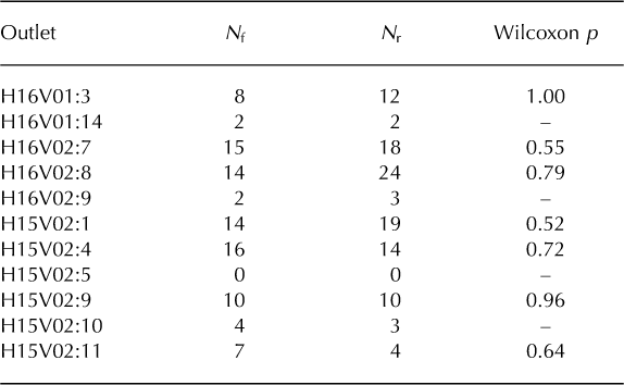
Plumes are classified according to whether they occur on a rising or a falling tide, then subjected to the nonparametric Wilcoxon (paired-difference) test with null hypothesis H 0 that diurnal and semi-diurnal tides do not influence plume area, at Pcritical = 0.05. Statistical tests of significance (Table 1) indicate that diurnal tide variations do not influence plume areas. All outlets report p-values from both t-tests and Wilcoxon tests far in excess of the critical value.
Results of Wilcoxon statistical test for effect of rising or falling tide on plume area. N f is number of plumes occurring on falling tide. N r is number of plumes occurring on rising tide. Where there are insufficient plume observations, no test is carried out. See Section 3.5 for Wilcoxon critical p-value.
4. Results
4.1. Outlets suitable for observations of plumes
Plume observations are restricted to days when acquisitions are sufficiently cloud/ice-free and of good quality (Fig. 1). Of the ˜46 000 observations attempted across the 36 outlets, ˜2200 were successful. The high proportion of acquisitions rejected by MODIS quality-assurance information illustrates the necessity of checking data integrity prior to quantitative analysis. Generally, larger outlets have a greater number of acceptable acquisitions. They appear less susceptible to exceeding the cloud-cover and quality thresholds. A number of smaller outlets (e.g. H15V02:2 and H15V02:3) are constantly cloudy or flagged for bad quality during the study period.
Summary of total accepted and rejected days for each outlet over the period 2000 – 07, organized by latitude (north at top of plot). ‘Quality rejected’ combines rejections from MOD09GQ and MOD10A1 quality assurance with corrupt or missing acquisitions. ‘Cloudy/icy’ combines cloud and ice flags. ‘Passed checks’ indicates the total days on which plume quantification is possible. Only those outlets with ‘passed checks’ depicted in solid black are retained for further analysis.

Of the original 36 outlets, 15 are retained. All higher-latitude outlets are marine-terminating, and all outlets below ˜67° N (Søndre Strømfjord) are land-terminating. Figure 2 shows a summary of the temporal resolution achieved at each retained outlet. Some outlets have better temporal resolution than others: marine-terminating higher-latitude outlets suffer from prolonged ice cover, inhibiting the observation of plumes until late in the melt season. Outlets midway along the west coast have a minimum of approximately weekly temporal resolution, usually with relatively even spacing during the melt season. Outlets in the southwest (e.g. H15V02:6 and H15V02:7) suffer more strongly from cloud cover, which significantly reduces the temporal resolution.
Summary of temporal resolution achieved for each retained outlet. Each individual observation is denoted by a vertical bar. The scale is discontinuous between years as observations are only made between days 121 and 273.
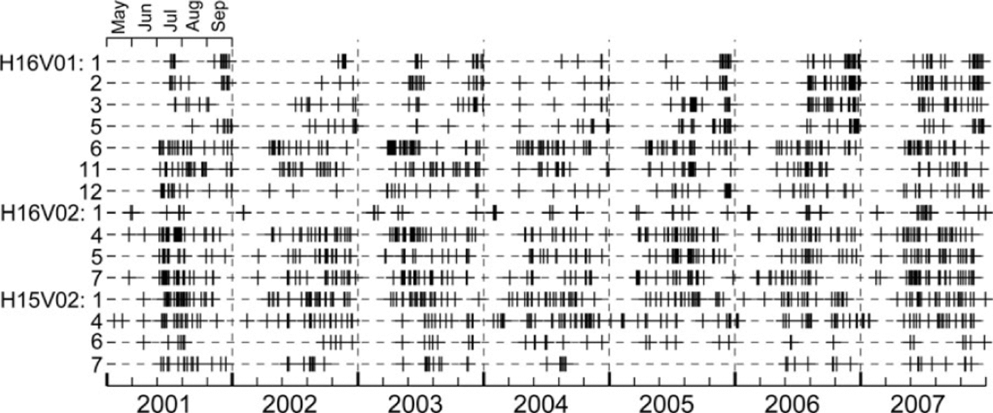
All acquisitions during 2000 failed quality or cloud checks. Subsequent analysis therefore only addresses observations from 2001 to 2007.
4.2. Validation
4.2.1. Søndre Strømfjord
Observations made by the system of plumes in Søndre Strømfjord (a land-terminating proglacial river outlet) are reproduced here (Fig. 3) for comparison with those obtained by Reference Chu, Smith, Rennermalm, Forster, Box and ReehChu and others (2009) and Reference McGrath, Steffen, Overeem, Mernild, Hasholt and Van den BroekeMcGrath and others (2010). Overall, automatic quantification successfully replicates previous findings at the wide, straight Søndre Strømfjord. There is strong correspondence in the patterns of plume size variability, both over periods of a few days and across each season. Our plume onset times are conservative in comparison, as we tend to make fewer observations early in the melt season due to poor imagery quality. Plume cessation times agree to within a few days, although Reference Chu, Smith, Rennermalm, Forster, Box and ReehChu and others (2009) manage observations later in the year when our system decides that the imagery is of insufficient quality. Our system makes a small number of additional observations during each season due to differing quality-control procedures.
Daily plume observations at outlet H15V02:1, 2001 – 07. Individual plume observations indicated by black filled circles. Absence of a black filled circle indicates that no observation was possible on that day. Solid line indicates SSM/I daily melt extent in the outlet’s hydrologic catchment.

High-quality observations are also made at other land-terminating outlets with similarly wide and straight fjord geometries, whether fed by a single proglacial river or via an outwash plain. In particular, runoff routed through outwash plains gives the appearance of coalescing into one point input and therefore a single plume at the spatial resolution of MODIS imagery.
4.2.2. Narrow outlets
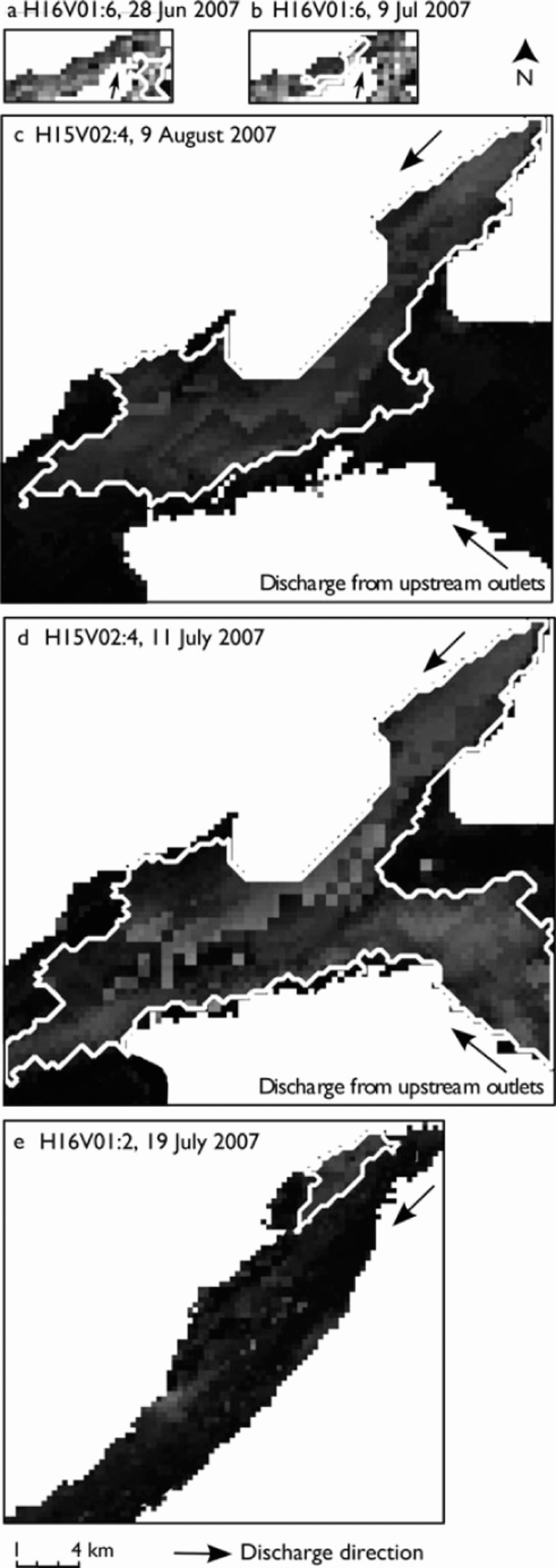
Plume identification in outlets narrower than ˜2km is inconsistent. Scrutiny of individual acquisitions reveals a high proportion of 'mixed pixels', making fjord margin delineation unclear. Spatially coherent plume areas are not easily identifiable. For instance, the plume in Figure 4a appears to continue northward by ˜5 pixels but is not wholly captured by the traced polygon. The polygon in Figure 4b does not appear to be representative of a plume. We therefore have low confidence in observations made of plumes in narrow outlets irrespective of their geometry classification.
Example plume traces (red polygon) from the outlets examined during validation. Outlets are masked from neighbouring land using our modified version of the MODIS land-water mask (Reference Carroll, Townshend, DiMiceli, Noojipady and SohlbergCarroll and others, 2009). Arrow indicates water discharge direction.
4.2.3. Multiple proglacial rivers discharging into one fjord
The plume emanating from the land-terminating proglacial river outlet H15V02:4 can be disturbed by plumes extending from two outlets further up-fjord. In many cases, the plume identified by the system is strongly associated with the river outlet of interest (e.g. Fig. 4c), justifying the need for plume identification to begin along the up-outlet edge of the image. However, plumes emanating from different rivers can combine downstream (e.g. Fig. 4d). There is potential for a seasonal overview of fluctuating plume areas to be ascertained, but at a higher degree of uncertainty than that associated with fjords fed by a single hydrological outlet.
4.2.4. Marine-terminating glacier outlets (bay and fjord)
Marine-terminating glaciers are very common further north along the west coast of Greenland. Visually, traced plume areas in front of marine-terminating ice fronts are generally representative of a small discrete plume exiting the terminus (e.g. Fig. 4e), in both bay and fjord settings, and appear within metres of the terminus as observed at Kangiata Nunata Sermia, southwest Greenland, by Reference SoleSole and others (2011) using time-lapse photography. Discrete, unconnected patches of sediment are sometimes visible further down-fjord. This highlights the importance of tracing plumes rather than simply taking the sum of all pixels in the outlet corresponding to sediment reflectivity, as tracing enables discrimination of plumes indicative of recent hydrologic discharge.
4.2.5. Outcomes of validation
The quality of automatic quantification is good overall. Examination of all outlets during 2007 indicates that the exemplar outlets presented above are representative of their respective outlet geometry classifications. Outlets with regular, wide and straight geometry are particularly satisfactory, while care is required when interpreting outlets where there are other river channels within a few kilometres or with enhanced likelihood of ice cover.
4.3 Annual variability in plume areas
At annual timescales, greater mean catchment melt extent is generally tracked by larger mean plume areas in the majority of outlets (Fig. 5). The degree to which plume areas change concomitantly with melt extent varies between years and outlets. H16V01:3 exhibits similar interannual relative changes between melt extent and plume area, but in most outlets the degree of change in plume areas compared to melt extent varies annually. This is especially visible throughout 2001-07 in H16V01:1, H16V01:6 and H16V01:11.
Interannual variations in mean annual melt extent (solid line, circle) and mean annual plume area (dashed line, square) for each retained outlet. Top bars over 2003 agree with high melting and runoff year (Reference HannaHanna and others, 2008; Reference EttemaEttema and others, 2009; Reference Mernild and HasholtMernild and others, 2009), and over 2005 – 07 indicate synchronous interannual variations in agreement with Reference EttemaEttema and others (2009) and Reference Mernild and HasholtMernild and others (2009). Outlet catchment areas are shaded in grey. Outlets are classified by geometry according to the schema in Section 2.
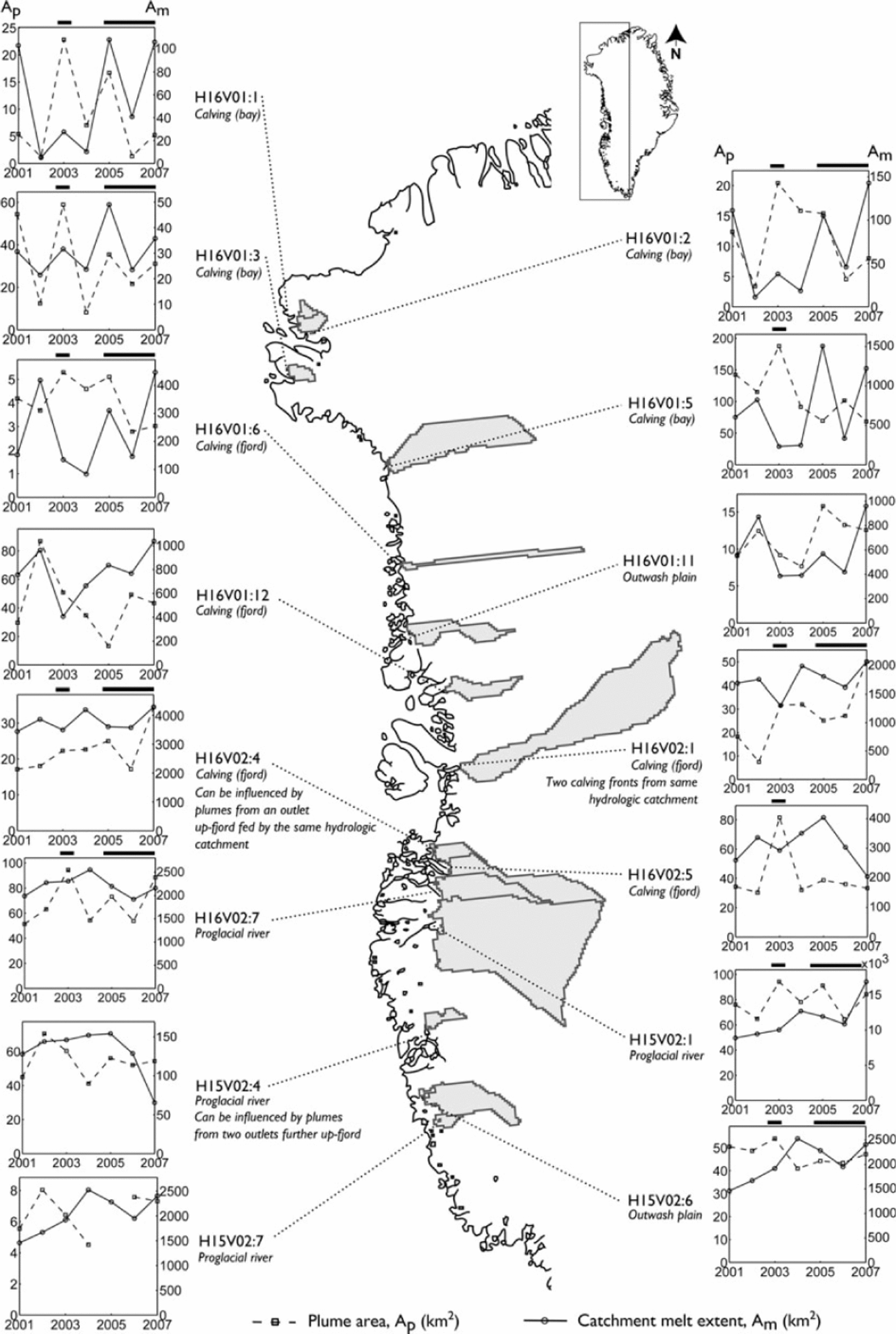
In some years and for some outlets there is no clear relationship between melt extent and plume areas: plume areas increase while melt extent decreases and vice versa. Examples include H16V01:6 in 2002 and 2003, and H16V02:7 in 2004. Moreover, this pattern is observed simultaneously in a number of lower-latitude outlets from 2003 to 2005: while melt increases from 2003 to 2004 and then drops by a lesser degree in 2005, plume areas drop significantly from 2003 to 2004 before increasing again in 2005. Outlets with this pattern include H16V02:7, H15V02:1, H15V02:4 and H15V02:6, all of which are land-terminating.
Synchronous interannual changes are also apparent in higher-latitude outlets, particularly between the neighbouring outlets H16V01:1, 2 and 3. In all three the directions of change in melt extent and plume area are the same. The patterns of change are replicated to a lesser extent in H16V01:5, H16V01:6 and H16V01:11.
Nine of the fifteen outlets show synchronicity during 2005-07 (top-barred in Fig. 5), irrespective of latitude or geometry classification. During this time, melt extent decreases from 2005 to 2006, then increases from 2006 to 2007, recovering to areas slightly less than those observed in 2005. Plume areas similarly decrease from 2005 to 2006, then increase from 2006 to 2007. The magnitude of changes in plume areas from year to year varies for each outlet. Melting and plume areas from some outlets (e.g. H16V01:12, H16V02:1, H15V02:1) show a net increase from 2005 to 2007, while others show a net decrease (e.g. H16V02:5, H15V02:4) or little net change (e.g. H16V02:7, H15V02:6).
Statistical tests also suggest synchronicity between outlets at annual timescales. Spearman's rank coefficient is calculated for each year using the mean annual plume area and mean annual catchment melt extent of each retained outlet (n = 15, apart from 2005 when n =14 as H15V02:7 was not observed). There is relatively strong positive correlation in 2002 (0.63, p = 0.01), 2004 (0.45, p = 0.08), 2006 (0.48, p = 0.06) and 2007 (0.56, p = 0.03). Coefficients for 2006 and 2007 suggest that the changes between 2005 and 2007 identified in the subset of nine outlets above are spatially widespread.
4.4. Short-term variability in plume areas
The extent to which changes in plume area coincide with short-term surface melt extent expansions is assessed for a subset of individual outlets and hydrologic catchments during periods when imagery quality permits daily or near-daily plume observations. We focus in particular on daily variability across a range of outlet geometry classifications.
High-latitude marine-terminating ice margins such as H16V01:1 (Fig. 6) are strongly affected by sea-ice presence in the bay into early summer, and also by frequent cloud cover. They exhibit little short-term covariation between melt extent and plume areas. During July 2001 and 2003, and August 2006, observed plume areas may be related to recent melt extent, but plumes such as those during July 2007 and August 2003 and 2004 – when no melting is identified – counteract such a relationship.
Daily plume observations at outlet H16V01:1, 2001 – 07. Legend as Figure 3. Specific to this figure, grey triangles indicate days on which ice is present in fjord, and plume areas are shown on a log10 scale.

Although plumes appear to be prevalent throughout much of September each year, they are not always coincident with ice-sheet surface melting. Only in September 2002 and September 2006 do observed plumes coincide with continuing melting. Manual verification of the observations suggests that sea ice or icebergs have not been quantified erroneously. Spot spectral measurements are however very low, at ˜5% (brackish water), and plumes do not have coherent high-reflectance cores. Observations late in the melt season should therefore be treated with caution.
Plume areas in H16V01:11, a land-terminating outwash plain outlet (Fig. 7), fluctuate significantly over short time periods, often varying simultaneously with melt extent. During melt onset in 2001, 2002 and 2007, plume areas are proportionally larger than they are during the remainder of the melt season. A number of larger plume areas coincide with spikes in melt extent: early July 2003, mid-/late July 2003 and late July 2006 are particularly clear. Plume areas tend to decline with decreasing melt extent from August.
Daily plume observations at outlet H16V01:11, 2001 – 07. Legend as Figure 3.

The temporal resolution of plume observations in the land-terminating proglacial river outlet H16V02:7 (Fig. 8) varies between years. The 2003, 2005 and 2007 melt seasons have observations at least once a week after plume onset, while 2004 and 2006 suffer from gaps of up to a month in observations. Plume areas generally vary with changes in melt extent during the preceding few days. Some periods have very good observation coverage, making it possible to examine short-term variability. During the first 2 weeks of July 2001, plume areas initially decrease, in response to a minor reduction in melt extent. They do not respond to the following increase in melt area, but do drop in response to its subsequent gradual decline over approximately 5 days. Plume areas then increase again within 2-3 days of the melt extent increasing into mid-July. Similarly, during July 2007, daily variations in plume area closely track increases in peak melt extent by 1-2 days and track a gradual upward trend in melt extent into mid-July. In years when plume observations are available later in the melt season they tend to co-vary with melt extent with little evidence of plume area hysteresis.
Daily plume observations at outlet H16V02:7, 2001 – 07. Legend as Figure 3.

5. Discussion
5.1. Feasibility of an automated remote-sensing approach
Automated observation of sediment plumes in MODIS satellite imagery is computationally feasible. Processing takes a matter of hours for the full set of 36 outlets from 2000 to 2007. While an automated approach undoubtedly brings its own errors and uncertainties, validation of observations made in 2007 suggests that automation is a viable compromise. It enables the flexible and rapid identification of plumes in a number of meltwater outlets simultaneously, without recourse to intensive manual processing, providing a spatially extensive dataset essentially unobtainable by other means. Rigorous imagery quality-control procedures increase the level of confidence in the automatic, unsupervised quantifications of plume areas.
However, a fundamental limit of sediment plume quantification remains the maximum MODIS resolution of 250 m. Most of the land-terminating outlets along the west coast of Greenland visible in MODIS imagery were examined during this study, apart from a few with short fjords or unsheltered bays that are more likely to be strongly affected by regional winds and ocean currents. The minimum channel width practical for examination is ˜2 km. Very narrow outlets such as H16V01:6 have too many mixed pixels for plume identification to be reliable. Plumes are thus more appropriate for identifying runoff from larger outlets.
Marine-terminating margins at higher latitudes have a propensity during September for large areas of brackish water, which at Reference McGrath, Steffen, Overeem, Mernild, Hasholt and Van den BroekeMcGrath and others' (2010) thresholds are (mis-)classified as plumes despite the requirement for a minimum number of pixels with 'plume core' reflectance. Further field campaigns to calibrate the spectral characteristics of plumes at these latitudes are desirable.
5.2. Impact of ice margin type and outlet geometry
The most accurate results are gained from land-terminating meltwater outlets with simple geometries fed by a single proglacial river. Land-terminating meltwater outlets with outwash plains between the ice terminus and fjord head are also reliable candidates for runoff quantification.
Sediment plumes as proxies for meltwater runoff are only of significant utility if they are representative of runoff from locations with more complex characteristics than Søndre Strømfjord.
-
1. Multiple meltwater sources. Some inferences about meltwater runoff may be drawn from locations with multiple meltwater sources if there is reasonable spatial separation between outlets; annual averages of plume areas are more instructive than comparisons of daily observations and seasonal averages to catchment melt extent. Examples include H16V02:1 and H16V02:4, but not H15V02:4, where plumes are produced by runoff from about four outlets and attenuated by intermediate storage in proglacial lakes.
-
2. Marine-terminating outlets (fjord and bay). Observations of plumes at slow-moving marine-terminating margins are usually successful, despite sporadic sea-ice interference and the potential for multiple forced-momentum plumes emanating from englacial and subglacial channels along the ice front. Multiple plumes are likely to coalesce rather than be individually discernible at 250 m resolution, thereby simplifying analysis. We cannot identify any systematic difference between plumes emanating from fjord versus bay outlets.
Automated quantification poses problems at fast, sensitive marine-terminating glaciers such as Jakobshavn Isbræ, where ice terminus locations can move by kilometres each year: our system requires a spatially fixed glacier/fjord boundary to simplify quality control. Associated high volumes of iceberg calving can interrupt otherwise coherent plumes, particularly as no band ratios suitable to delineate plumes can be employed with MODIS 250 m imagery (Reference Chu, Smith, Rennermalm, Forster, Box and ReehChu and others, 2009). The present study's approach to automatic quantification of sediment plumes is therefore of most utility for meltwater outlets with minimal sea ice and iceberg presence and relatively static outlet geometries.
-
3. Variable water-routing lag times. Lags between melting and subsequent runoff to the ocean are introduced not only by drainage through the ice sheet but also by the distance from the ice margin to the outlet. At outlets fed by land-terminating glaciers the lag can be >24 hours (e.g. Søndre Strømfjord; Reference McGrath, Steffen, Overeem, Mernild, Hasholt and Van den BroekeMcGrath and others, 2010).
5.3. Runoff from individual catchments
At annual timescales, sediment plumes tend to track surface melting in their catchment. At many outlets it is therefore clear that surface meltwater production is proportional to plume area, although the relationship is unique to each outlet. We believe that, so long as daily plume observations are spaced relatively evenly across the runoff hydrograph of the whole melt season, the precise day on which the observation is made does not matter. Proglacial discharge records (e.g. from Leverett Glacier, southwest Greenland (Reference BartholomewBartholomew and others, 2011, fig. 2a)) clearly show that variability in runoff on individual days is dwarfed by the magnitude of the overall seasonal trend in runoff. However, we do lack the near-daily temporal resolution required to accurately determine runoff onset and cessation.
Seasonality in plume areas at Søndre Strømfjord was identified by Reference Chu, Smith, Rennermalm, Forster, Box and ReehChu and others (2009). They calculated the means of daily plume area observations from 2000 to 2007, from a dataset of similar temporal resolution to that observed here. While their conclusions appear to be reasonable, it is worth noting the amount of obfuscation introduced by the use of daily means: the seasonal box-plot of plume areas in Søndre Strømfjord (Fig. 9) illustrates that plume areas on specific days can vary by an order of magnitude from year to year. Moreover, many daily averages are calculated from only two observations, reducing the significance of any seasonal trends inferred from the mean time series. However, a number of lower-latitude catchments show some indication of seasonal sediment-supply hysteresis similar to that identified at Søndre Strømfjord by Reference Chu, Smith, Rennermalm, Forster, Box and ReehChu and others (2009).
H15V02:1 (Søndre Strømfjord). Seasonal variation in plume areas over 2001 – 07 shown as box-plots on days when observations from multiple years are available. Daily melt extent calculated as a daily mean from 2001 to 2007.

At higher latitudes, plume areas show very little relationship to daily surface melt extent. All higher-latitude outlets are marine-terminating. Plume evolution is therefore likely to be controlled by different processes from those operating at land-terminating outlets, as water tends to be discharged as a forced momentum plume at depth directly from englacial and subglacial conduits and disperses vertically through the water column as the more buoyant fresh water rises to the fjord surface (Reference Mugford and DowdeswellMugford and Dowdeswell, 2011). More sediment is therefore likely to be required to produce a visible plume in the uppermost layers of the water column compared to a land-terminating outlet, and may explain the brackish waters visible late in the melt season. Plume areas in neighbouring outlets H16V01:1, H16V01:2 and H16V01:3 all react similarly to varying melt extent, which suggests that the forced momentum delivery mechanism of plumes does not vary significantly between glaciers. However, the poor quality of imagery throughout most of the melt season at high latitudes prevents us from further examining the differences between forced-momentum and buoyant plumes. We also note that hyperpycnal plumes (entering the fjord or bay as underflows) are unlikely, as fresh water is seldom of sufficient density, even with the high SSCs present in glacial meltwater runoff (Reference Mugford and DowdeswellMugford and Dowdeswell, 2011).
The brackish-water spectral reflectance of many of the observed plumes at higher latitudes may alternatively be a result of slow delayed discharge from the subglacial environment as surface meltwater from earlier in the season gradually and inefficiently flows through cavity systems. However, higher spectral reflectances might be expected due to the high degree of bed contact. Alternatively, they could be associated with the marine mixing of (unobserved) plumes emanating during August. These observations therefore remain unexplained, and may not be physically representative of ice-sheet runoff.
At lower latitudes, plume areas vary substantially from one day to the next. During periods of near-daily observations, plume areas are observed to fluctuate by up to ˜50% of their peak size, for example at H16V01:1 (Fig. 6), H16V01:11 (Fig. 7) and H16V02:7 (Fig. 8). Daily fluctuations in plume areas and surface melt extent often co-vary. These suggest that sediment plumes are good proxies for episodes of elevated meltwater release from the ice-sheet surface over periods of a few days once lags due to water routed subglacially (and in land-terminating cases also proglacially) are allowed for. The concomitant variability is stronger in outlets with simple outlet geometries and large catchment areas such as H16V02:7.
Plume area contractions from one day to the next associated with reductions in surface melt extent suggest that the distal sections of sediment plumes mix relatively rapidly with the marine water body and move quickly downstream. This enables the primary causes of plume expansion and contraction to be ascribed to variations in the runoff of ice-sheet surface meltwater. If a plume were to persist by more than a few days beyond a strong decline in melt extent, it could no longer be physically representative of subsequent runoff. Averaged over the whole melt season, if plumes were not to mix relatively rapidly then they would become far less sensitive indicators of runoff and would incorrectly increase the inferred volume of runoff.
5.4. Spatio-temporal trends in runoff
Annually, many catchments show latitudinal synchronous average variations in surface melt extent and plume area. Significant correlation spatially suggests that plume area is strongly related to the magnitude of surface melting on an annual basis. Moreover, this indicates that catchments at the highest latitudes are also vulnerable to elevated mass losses by runoff, although field observations are required to confirm this. Thus, irrespective of seasonal lags in routing from the ice-sheet surface to the ocean, at annual timescales the requisite hydrological routing pathways are present all around the western margins of the Greenland ice sheet.
Synchronicity between catchments is less apparent at seasonal timescales as local climate and plume dynamics become increasingly important. However, plumes do appear to occur for longer on average at lower latitudes than at higher latitudes. This is as expected given that the melt season is longer at lower latitudes.
At all latitudes the first plumes tend to appear within a few days of mean melt onset (allowing for the long ice-margin-to-outlet distance of outlets such as H15V02:7). Seasonal exhaustion of the activated sediment supply is likely to be widespread, with the exception of the highest-latitude catchments. Theoretically, hysteresis could occur earlier in catchments where melting begins earlier, as sediment supplies should be exhausted more quickly, but such a trend cannot be identified in the observations. Any sediment-supply hysteresis is likely to be highly dependent on the frequency and extent of changes in subglacial hydrological routing – opening new sediment reserves – and the local ice-sheet bed characteristics.
At daily timescales it is clear that plume areas predominantly respond to catchment-scale short-term variations in melt extent. Most catchments, other than those at the highest latitudes, produce plumes from melt onset until the onset of sediment-supply hysteresis that track the relative magnitude of melt extent variability over the preceding ˜1-5 days. However, differences in lag times between catchments cannot be identified for a number of reasons:
-
1. Local conditions. Despite the apparent speed at which plumes disperse, plume mixing is likely to depend strongly on local conditions. These include fjord geometry, internal tides and daily wind conditions, which serve to modify the cumulative runoff volume represented by a plume at any one point in time.
-
2. Distances. Distances between the ice margin and the outlet vary for each outlet and can introduce significant lags between surface melting and its subsequent arrival at the outlet.
-
3. Sediment sources and sinks. Outwash plains have been observed to act as net sediment sources earlier in the melt season, switching to net sediment sinks later on (Reference Hodson, Gurnell, Tranter, Bogen, Hagen and ClarkeHodson and others, 1998). Proglacial channel routing is therefore not conservative with respect to SSCs. Thus, the greatest utility of daily plume area observations appears to be for assessing runoff variability as a function of climatological variables or bulk indicators such as surface melt extent.
5.5. Comparison to modelled meltwater runoff from Greenland, 2001 –07
While the total mass balance of the Greenland ice sheet has become increasingly negative during the last decade (e.g. Reference Pritchard, Arthern, Vaughan and EdwardsPritchard and others, 2009), the constituent components of mass loss – split between meltwater runoff and calving-vary significantly between years. Many surface mass-balance estimates use positive degree-day modelling to identify the runoff component. They typically include snowpack retention schemes and parameterizations based on calibration observations (e.g. Reference Hanna, Huybrechts, Janssens, Cappelen, Steffen and StephensHanna and others, 2005, 2008; Reference BoxBox and others, 2006). These are distinct from approaches such as SnowModel (Reference Liston and ElderListon and Elder, 2006) and RACMO2/GR (Regional Atmospheric Climate Model; Reference EttemaEttema and others, 2009), which estimate runoff quantities via physical modelling of the surface energy balance and snowpack evolution.
Annual averages of plume areas may be compared to these model-based estimates of runoff (Fig. 10; see also individual outlets in Fig. 5). The year 2007 had record melting (Reference MoteMote, 2007) which was captured by SnowModel (Reference Mernild and HasholtMernild and others, 2009), while Reference EttemaEttema and others (2009) attribute the RACMO2/GR non-record 2007 runoff volume to a cold 2006/07 winter that enhanced springtime refreezing despite record melting. Plume areas during 2007, while large at a number of outlets, are not generally the largest in the 7 year time series, and therefore tend to agree with the RACMO2/GR runoff results. The high-runoff year of 2003 (top-barred in Fig. 5) is clearly visible in plume observations: plumes at the majority of outlets are relatively smaller during 2001 and 2002 compared to 2003, before dropping abruptly in 2004.
Comparison of (a) annual plume sizes (mean of observed plumes in all 15 outlets each year) with (b) estimates of runoff by other approaches: degree-day modelling (Reference HannaHanna and others, 2008), RACMO2/GR (Reference EttemaEttema and others, 2009) and SnowModel (Reference Mernild and HasholtMernild and others, 2009).
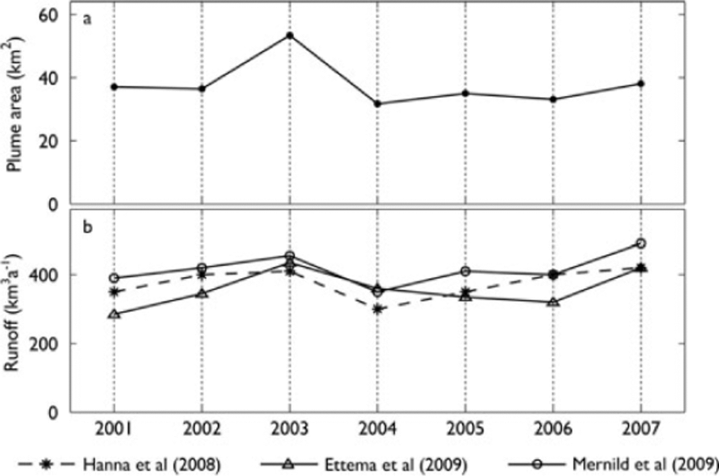
Observations of plume areas from 2005 to 2007 in the nine outlets shown in Figure 4 tend to agree more favourably with SnowModel and RACMO2/GR estimates of runoff than those based on degree-day modelling. Specifically, 2006 is identified by snowpack evolution modelling and plume observations as a lower-runoff year, while degree-day models show an increase on 2005 runoff, despite temperatures during 2005 and 2007 being higher than those in 2006 (Reference HannaHanna and others, 2008). The degree-day model 2006 results are attributed to low winter snow accumulation and higher summer temperatures, but with the caveat that the snowpack energy balance, precipitation and timing of summer melt events all modulate the parameterized accumulation-ablation relationship of the degree-day model (Reference HannaHanna and others, 2008).
As physical energy-balance models specifically account for the physical processes only parameterized by degree-day models, it is encouraging that interannual plume observations track estimates based on physical snowpack evolution. These plume observations additionally highlight the importance of employing rigorous, physically based highresolution surface mass-balance models to estimate runoff from the Greenland ice sheet.
6. Conclusions
Automated quantification of sediment plumes in MODIS satellite imagery is feasible in meltwater outlets wider than ˜2 km. Widespread cloud cover and bad imagery quality reduce the temporal resolution of plume observations significantly. At many outlets there are insufficient observations to constrain meltwater runoff onset, duration and variability. Reference Chu, Smith, Rennermalm, Forster, Box and ReehChu and others (2009) and Reference McGrath, Steffen, Overeem, Mernild, Hasholt and Van den BroekeMcGrath and others (2010) may have overstated their cases for the wider application of sediment plumes as runoff proxies for individual hydrologic catchments: Søndre Strømfjord is one of the widest and straightest outlets in Greenland, supplied primarily by one proglacial river channel flowing from the land-terminating ice margin. Marine-terminating ice margins, narrow and complex geometries or multiple meltwater outlets all introduce uncertainty as they modulate or disrupt plume fluid dynamics.
Despite these caveats, annual plume areas usually track annual variations in melt extent. Thus, in years of more extensive melting, more mass is lost by meltwater runoff. In a number of years, statistically significant synchronicity between plume areas in different outlets is apparent. At many outlets there is good annual correspondence with runoff modelled by SnowModel (Reference Mernild and HasholtMernild and others, 2009) and RACMO2/GR (Reference EttemaEttema and others, 2009), confirming that sediment plumes are a valid proxy for annual meltwater runoff from the Greenland ice sheet.
Plumes emanating from outlets with just one runoff source (e.g. a single proglacial river) and relatively straight geometries tend to track the evolution of surface melt extent over the course of the melt season, with minimal lags. There is substantial variability in seasonal behaviour each year. Average runoff onset dates tend to be earlier in the year and to continue throughout the summer at lower latitudes, unlike at higher latitudes where runoff is generally more episodic.
Daily variability in plume areas predominantly tracks changes in the magnitude of surface melt extent in the associated catchment. Plumes can expand or contract from one day to the next.
Overall, sediment plumes show promise as a means of constraining meltwater runoff from individual meltwater outlets around Greenland, albeit limited to larger outlets. Under the approach adopted here, their utility lies principally at the annual timescale. Plumes appear to react to short-term fluctuations in surface melting and thus may be relatively sensitive indicators of changing ice-sheet hydrology over periods of days or more. Future research should seek to examine in more detail the relationship of plume areas to ice-sheet melting and hydrological routing, primarily via additional field campaigns at a variety of meltwater outlets, including at marine-terminating glacier fronts.
Acknowledgements
A.T. was funded by Fitzwilliam College, Cambridge. We thank P. Christoffersen and M. Bithell for computing facilities and T. Benham for cartographic resources. We also thank V. Chu and an anonymous reviewer for helpful reviews.



