

Introduction
Knowledge of ice-flow velocity and Strain rate is important in assessing an ice sheet’s mass balance and in understanding its flow dynamics. Ground-based measurements of ice-sheet velocities are scarce because of logistical and technical difficulties. Ice-flow velocities have been measured from the displacement of features observed in pairs of visible (Reference Scambos,, Dukiewicz,, Wilson, and Bindschadler,Scambos and others. 1992; Reference Ferrigno,, Lucchitta,, Mullins,, Allison,, Allen, and Gould,Ferrigno and others. 1993) or synthetic aperture radar (SAR) images (Reference Fahnestock, Bindschadler,, Kwok and JezekFahneslock and others, 1993), but these methods do not work well for the large, featureless areas that comprise much of the ice sheets.
Several recent papers have indicated that satellite radar interferometry (SRI) provides a potential means to measure ice-flow velocity. Using SRI, Reference Goldstein,, Engelhardt,, Kamb and Frolich,Goldstein and others (1993) estimated ice velocity for an area on the Rutford Ice Stream. Antarctica. Interferograms of the Hemmen Ice Rise on the Filchner-Ronne Ice Shelf have been studied by Reference Hartl,, Thiel,, Wu,, Doake, and SieversHartl and others (1991). Reference Joughin,Joughin and other (1995) have examined interlerograms from a 400km long area on the Greenland ice sheet that exhibit complex phase patterns due to ice motion. Agreement between interferometric and in situ measurements of velocity, was obtained by Reference Rignot,, Jezek, and Sohn,Rignot and others (1995). Reference Kwok, and Fahnestock,Kwok and Fahnestock (1996) have measured relative velocity on an ice stream in Greenland.
While these papers have demonstrated the great potential of SRI for measuring ice-sheet motion, the results of these studies are subject to error due to difficulty in estimating the interferometric baseline (i.e., the separation of points from which two images are acquired). Estimates of the baseline determined from satellite ephemeris data, derived from satellite tracking and orbital modelling, are typically accurate to within a few meters (Reference Solaas,Solaas,. 1991). While adequate for many purposes, this level of accuracy can introduce substantial error in motion estimates. For example, a 1 m error in the baseline can introduce a phase ramp of about four fringes across a 100 km wide interferogram. yielding a relative velocity error of 39 m year−1 for a 3 d separation of images. Tie points (points of known elevalioti and velocity) can be used to improve the accuracy of baseline estimates (Reference Zebker,, Werner,, Rosen, and HensleyZebker and others. 1994), Because estimates of baselines from orbital data alone are unlikely to yield reasonable accuracy, wide-scale mapping of ice-sheet velocities requires a combination of interferometric data and tie points determined from global positioning system (GPS) or other field-based surveys. The cost of measuring such tie points is high. Thus, it is important to understand how to select tie points to achieve maximum accuracy at minimum cost.
We begin with a brief introduction to interferometric principles and techniques. The next section describes an error model for SRI velocity estimation. The results of simulations are then examined to determine how baseline accuracy is affected by various factors. Velocity errors are examined for two typical situations that are likely to occur in measuring ice-sheet motion. Next a method is developed to improve estimation of horizontal velocity by compensating for the effect of vertical motion using interferometrically derived estimates of the surface topography. We then apply this technique to estimate the single-component velocity field for an area on Humboldt Glacier. Greenland. Our results confirm that SRI provides an important new means for measuring ice velocity, as indicated by earlier studies, and that a small number of field-determined motion and elevation tie points will allow production of calibrated maps of ice-flow speed covering thousands of square kilometers.
Interferometry Background
The geometry of an interferometric SAR is shown in Figure 1. The interferometer acquires two images of the same scene with SARs located at S1 and S2. The first SAR is at altitude H. From S1, the range, r0 , and look angle, θ, to a point on the surface are determined by the ground range, y, and elevation, z, above some reference ellipsoid. The range to the same point from the SAR at S2 differs from r0 by Δ. For a single-pass System, such as TOPSAR (Zobker and others. 1992), two images are acquired simltaeously using separate antennas. A repeat-pass interferometer, on the other hand, acquires a single image of the same area twice from two nearly repeating orbits or flight lines. Only repeat-pass interferometry is examined in this paper since so far this is the only method that has been applied to orbiting SARs. The baseline separating the SARs can be expressed in terms of its components normal to, Bn , and parallel to, Bp, a reference-look direction. A convenient choice is to let the nominal center-look angle, θc, define the reference-look direction.
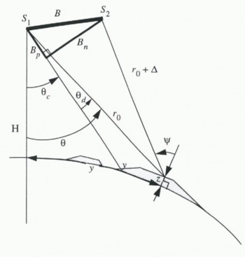
Fig. 1. Geometry of an interferometric SAR.
For a distributed target a pixel in a complex image can be represented as
where k is the wave number and W1 is a complex, circular Gaussian random variable (RV) with amplitude A1 and phase ϕ1 (Reference Rodriguez, and Martin,Rodriguez, and Martin. 1992). This random variation of SAR amplitude and phase is referred to as speckle. The modulo-2π phase from a single complex image cannot be used to determine range since it has a uniform probability distribution over (0, 2π). A complex interferogram is formed as the product of one complex SAR image with the complex conjugate of a second. The phase of this product is given by
Although ϕ1 and ϕ2 are both uniformly distributed, if W1 and W2 are correlated, their difference. (ϕ1−ϕ2), is not uniformly distributed. In fact, the distribution of the phase difference can be quite sharply peaked (i.e., there is little noise) if the complex images are well correlated.
Even with a narrow distribution, the phase difference is still only known modulo 2π. A phase-unwrapping algorithm (Reference Goldstein,, Engelhardt,, Kamb and Frolich,Goldstein and others, 1988) is used to remove the modulo-2π ambiguity. With repeat-pass interferometry, the range difference between passes is determined using
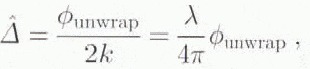
where ϕunwrap denotes the unwrapped interferometricphase difference and λ is the radar wavelength. Error in this estimate is introduced by (ϕ1 − ϕ2). Note that phase-unwrapping algorithms usually yield the relative phase, as there is an unknown constant of integration associated with the unwrapped solution. It is assumed here that ϕunwrap has been processed to remove this ambiguity (with the aid of tie points). The ERS-1 SAR operates at a wavelength of λ = 5.656 cm so that Δ typically can be measured with sub-centimeter accuracy.
With a repeat-pass interferometer, Δ is affected by both topography and any movement of the surface that is directed toward or away from the look direction of the radar between orbits. The interferometric phase therefore can be expressed as the sum of displacement- and topography-dependent terms,
Motion
The contribution to the overall phase from surface displacement is given by
where Δd,y denotes the component of the range difference tangential to the surface of a reference ellipsoid that is directed across track, and Δd,z denotes the component normal to the- ellipsoid. The incidence angle. ψ, is defined with respect to the local normal to the ellipsoid (see Fig. 1). When the surface velocity does not change over the period, δT, between acquisition of images, the phase due to motion is
Topography
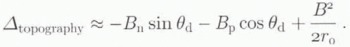
Referring to Figure 1, the baseline is related to the range difference due to topography and ground-range variation, Δtopography , by
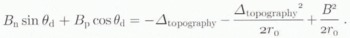
Ignoring the  term in Equation (7), we can approximate the range difference by
The deviation of the look angle from the center-look angle, θd , is related to range and surface elevation referenced to a spherical Earth by

where Re denotes the radius of the Earth. Once Δtopography is determined from the phase. Equation (7) and (9) are solved to determine the height and ground range of each point in the image (Reference Li, and Goldstein,Li and Goldstein, 1990).
There is a nearly linear phase variation, which is much greater in magnitude than the phase variation due to topography, from the uniform change in ground range, y, across an image. It is often useful to remove the ground-range variation by subtracting the phase ramp, ϕflat, corresponding to a zero-height surface. This operation is often called flattening the interferogram. The effect of elevation on the interferometric phase can then be approximated as (Reference Joughin,Joughin, 1995)
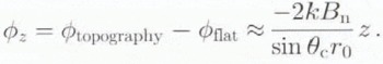
This approximation, which is not valid for computing elevations, indicates that the sensitivity of an interferometer to topography is proportional to Bn . Thus, when we refer to the baseline length below, we mean the length of Bn , rather than the actual baseline length. B.
Baseline estimation
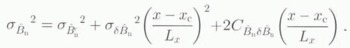
ERS-1 orbits are not known well enough to estimate baselines with the level of accuracy needed to generate digital elevation models (DEMs) and estimate motion. As a result, the baseline must be determined using tie points (Reference Zebker,, Werner,, Rosen, and HensleyZebker and others, 1994). The baseline varies along the satellite track. Over the length of an ERS-1 interferogram, we model baseline variation as a linear function of the along-track coordinate, x. The normal component of baseline is then represented as
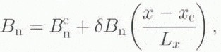
where ![]() is the normal component of baseline at the frame center, xc
, and δBn
is the change in Bn
over the length of the frame, Lx
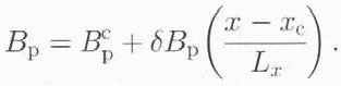
. Similarly, the parallel component of baseline can lie modeled as
is the normal component of baseline at the frame center, xc
, and δBn
is the change in Bn
over the length of the frame, Lx
. Similarly, the parallel component of baseline can lie modeled as
With a linear model for baseline variation, there are four unknown parameters: ![]() . There is also an unknown constant associated with the phase after it has been unwrapped. An approximation can be made to implicitly incorporate this constant into the baseline solution so that only the four baseline parameters need to be determined (Reference Joughin,Joughin, 1995). The expression given by Equation (7) is non-linear with respect to these parameters. The problem is easily linearized by replacing the non-linear terms, which are small, with estimates of their values obtained from satellite ephemeris data. The baseline parameters then are determined using a standard linear least-squares algorithm (Reference Press,, Flannery,, Teukolsky, and Vetterling,Press and others, 1992) with at least four tie points.
. There is also an unknown constant associated with the phase after it has been unwrapped. An approximation can be made to implicitly incorporate this constant into the baseline solution so that only the four baseline parameters need to be determined (Reference Joughin,Joughin, 1995). The expression given by Equation (7) is non-linear with respect to these parameters. The problem is easily linearized by replacing the non-linear terms, which are small, with estimates of their values obtained from satellite ephemeris data. The baseline parameters then are determined using a standard linear least-squares algorithm (Reference Press,, Flannery,, Teukolsky, and Vetterling,Press and others, 1992) with at least four tie points.
Even if the baseline were determined perfectly (so that the baseline estimate contributes no error to the velocity estimate), the estimated baseline would differ slightly from the actual baseline. This is because approximations in the baseline model and errors in some of the independent parameters (i.e., satellite altitude) are compensated for by using an effective rather than exact baseline. The difference between the true and effective baseline length is small.
Motion-estimation Error
Error model
The effect of topography must be removed from an interferogram before velocity estimates can be made. With a nearly zero baseline, the effect of topography is negligible and can be ignored (Reference Goldstein,, Engelhardt,, Kamb and Frolich,Goldstein and others, 1993). For longer baselines an independent DEM can be used to estimate and remove ϕtopography (Reference Massonnct.Massonnet and others, 1993). An alternative method is to cancel ϕtopography using an appropriately scaled topography-only interferogram (Reference Gabrial,, Goldstein, and Zebker,Gabriel and others, 1989). In this paper we use interferometrically derived DEMs to remove topographic phase variation.
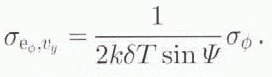
Interferograms are subject to random phase error due to speckle, σϕ, If the effect of vertical velocity is ignored, then applying Equation (6), the velocity error due to phase noise is
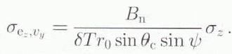
Estimates of ϕdisplacement are affected by inaccuracy in the DEM used to estimate ϕtopography . Using Equation (10), the standard deviation of this error is expressed as
where σz denotes the standard deviation of the DEM error. Since this error is proportional to baseline length, its effect is negligible for sufficiently small baselines (Reference Goldstein,, Engelhardt,, Kamb and Frolich,Goldstein and others, 1993). If we ignore the v-z term in Equation (6), then the error in the velocity estimate is given by
For typical ERS-1 parameters this error is equal to 0.00106 B nσ z for a 3 d interferogram. A 50 m baseline and a DEM error of 50 m then would yield a velocity error of 2.6 m year−1.
In cancelling the topography the baseline-dependent phase ramp due to ground range (ϕflat) is also removed. Thus, inaccurate baselines lead to error through the imperfect cancellation of this elevation-independent phase variation. If the estimated baseline components are denoted as ![]() and
and ![]() , then applying Equation (8) and neglecting small non-linear terms, the resulting phase error is
, then applying Equation (8) and neglecting small non-linear terms, the resulting phase error is

where θ d,flat is evaluated via Equation (9) with z = 0. The variance of the error is
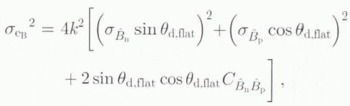
where ![]() denotes the covariance of
denotes the covariance of ![]() and
and ![]() . If we ignore the vertical component of velocity in Equation (6), the variance of the error in Vy
due to baseline inaccuracy is
. If we ignore the vertical component of velocity in Equation (6), the variance of the error in Vy
due to baseline inaccuracy is

This is often the largest source of error in interferometric estimates of ice velocity.
Applying Equation (11), the variance of the linearly varying baseline estimate can be expressed as
We may also write a similar expression for ![]() . The covariance between baseline components is given by
. The covariance between baseline components is given by

These expressions are used in Equation (18) to determine velocity error due to baseline inaccuracy.
The absolute error at any given point in the estimated velocity field is a random variable since it is a function of the random baseline error. Since the error is determined by only four parameters, however, it does not vary independently over the interferogram. At each point along track, error in the baseline estimate consists of a constant bias and nearly linear across-track tilt, which vary along track. As a result, the relative error from one side of the track to the other is roughly equal to the sum of the absolute errors at each side of the track. This should be kept in mind when interpreting results computed using Equation (18).
Accuracy of baseline estimates
In this subsection we examine the accuracy of baseline estimates using synthetic interferograms. Because it is often difficult to obtain tie points, it is important to understand how their number, accuracy and distribution affect baseline accuracy and, thus, the accuracy of velocity estimates. With this knowledge, optimal tie-pointing strategies can be devised to minimize field effort.
For the simulations we used a 303.2 km long by 100 km wide DEM of typical ice-sheet and bedrock (ice-free) topography. From the DEM we generated synthetic interferograms for several baseline lengths. All of the tie points are assumed to be stationary (i.e., located on bedrock). Non-stationary tie points (i.e., points on the ice sheet are examined in the next subsection. Noise was added to the tie points and to the interferogram. Baselines were estimated using a least-squares algorithm (Reference Press,, Flannery,, Teukolsky, and Vetterling,Press and others, 1992; Reference Joughin,Joughin, 1995). For each simulation, statistics were evaluated for the baseline estimates from 250 realizations. Because several parameters contribute tо baseline accuracy, there is no way here of illustrating baseline accuracy for all possible sets of parameters. In each of the simulations a single parameter is varied while the others are held fixed. The results will change w hen the other parameters are no longer fixed, although the trends should be similar.
The first simulation was performed to determine the effect of baseline length on estimation accuracy. For several baseline lengths we computed estimates for Gaussian phase noise of σϕ = 0 rad and σϕ = π/3 rad and Gaussian tie-point error of σz = 20 m. One hundred tie points (N ties = 100), evenly spaced over an area Dy = 86.9 km wide by Dx = 85.8 km long, were used. Standard deviations of the estimated parameters arc shown in Figure 2.
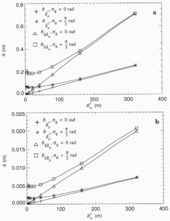
Fig. 2. Standard deviations of (a) ![]() (b)
(b) ![]() , and
, and ![]() for 250 estimates as a function of Bn. Estimates were made for Nties = 100, σz = 20 m, δBn = 0,
for 250 estimates as a function of Bn. Estimates were made for Nties = 100, σz = 20 m, δBn = 0, ![]() , δBp = 0, Dy = 86.9 km, Dx = 85.8 km and Lx = 303.2 km.
, δBp = 0, Dy = 86.9 km, Dx = 85.8 km and Lx = 303.2 km.
With no phase noise, baseline error increases linearly with Bn , because an interferometer with a shorter baseline is less sensitive to topography so that the effect of tie-point error is smaller. When there is phase noise, estimation accuracy improves with decreasing baseline length until a point where there is little further improvement. This point occurs where the effect of phase noise on baseline accuracy, which is independent of baseline length, becomes larger than that of tie-point error. Thus, the amount of improvement that can be gained by using a shorter baseline is limited by the amount of phase noise relative to the amount of elevation tie-point error.
Baseline estimates can be improved by using more than the minimum of four tie points in the least-squares solution (Reference Zebker,, Werner,, Rosen, and HensleyZebker and others. 1994). Figure 3 illustrates the standard deviation of the estimates of ![]() and
and ![]() as a function of the number of tie points, Nties
. The tie points are arranged on a regular grid Dy
= 86.9 km by Dx
= 85.8 km. Each time Nties
is increased, the spacing between points is decreased so that area covered by the tie points remains unchanged. The squared error for the fits (not shown) falls off as
as a function of the number of tie points, Nties
. The tie points are arranged on a regular grid Dy
= 86.9 km by Dx
= 85.8 km. Each time Nties
is increased, the spacing between points is decreased so that area covered by the tie points remains unchanged. The squared error for the fits (not shown) falls off as ![]() . In general, the standard deviations of the parameter estimates, including those not shown in Figure 3, decrease as
. In general, the standard deviations of the parameter estimates, including those not shown in Figure 3, decrease as ![]() . An exception is seen in Figure 3, where
. An exception is seen in Figure 3, where ![]() increases when Nties
increases from 4 to 9. The squared error for the overall fit, however, still decreases as expected.
increases when Nties
increases from 4 to 9. The squared error for the overall fit, however, still decreases as expected.
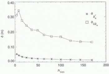
Fig. 3. Standard deviations of ![]() and
and ![]() for 250 estimates as a function of the number of tie points, Nties, for
for 250 estimates as a function of the number of tie points, Nties, for ![]() δBp = 0, Dy = 86.9 km, Dx = 85.8 km, Lx = 303.2 km, σϕ = π/3 rad and σz = 20 m.
δBp = 0, Dy = 86.9 km, Dx = 85.8 km, Lx = 303.2 km, σϕ = π/3 rad and σz = 20 m.
For a fixed number of tie points, the area bounded by the points affects the accuracy of baseline estimates. To examine this dependence, we used four tie points arranged to form a rectangle (Dy
by Dx) with sides parallel to those of the swath. Figure 4 shows the results plotted as a function of the product. Dy × Dx
. Each time Dx
and Dy
were increased, they were scaled by the same factor, except for the last two points where only Dx
was scaled because Dy
could not be scaled further without exceeding the swath width. The primary effect of ![]() on the interferometric phase is to determine a constant bias so that the estimate of this parameter is insensitive to tie-point spacing, as can be seen from the results in Figure 4. Error in the estimate of a derivative is inversely proportional to the distance between points. Consequently, the error in the estimate
on the interferometric phase is to determine a constant bias so that the estimate of this parameter is insensitive to tie-point spacing, as can be seen from the results in Figure 4. Error in the estimate of a derivative is inversely proportional to the distance between points. Consequently, the error in the estimate ![]() decreases as
decreases as ![]() , as illustrated in Figure 4. Likewise,
, as illustrated in Figure 4. Likewise, ![]() is inversely proportional to Dy
since Bn
determines the slope of the phase ramp across an interferogram. Finally. δBn
determines variation of the baseline with respect to x and also affects the slope of the phase ramp so that error in its estimate is inversely proportional to Dy × Dx
. Because increasing tie-point spacing affects the errors for each of the estimates differently, it is difficult to say exactly how the quality of the overall fit improves. It is clear, however, that increasing the distance between tie points significantly reduces error. A specific example is given in the next subsection.
is inversely proportional to Dy
since Bn
determines the slope of the phase ramp across an interferogram. Finally. δBn
determines variation of the baseline with respect to x and also affects the slope of the phase ramp so that error in its estimate is inversely proportional to Dy × Dx
. Because increasing tie-point spacing affects the errors for each of the estimates differently, it is difficult to say exactly how the quality of the overall fit improves. It is clear, however, that increasing the distance between tie points significantly reduces error. A specific example is given in the next subsection.
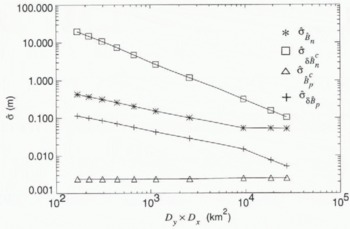
Fig. 4. Standard deviations from 250 estimates of the baseline parameters as a function of area covered by four tie points. Results are for ![]() 25 m, δBp = 0 m, Lx = 303.2 km, σϕ = π/3 rad and σz = 20 m.
25 m, δBp = 0 m, Lx = 303.2 km, σϕ = π/3 rad and σz = 20 m.
Error in the baseline estimates is caused by phase and tie-point noise. Figure 5 shows baseline error as a function of tie-point error for a fixed level of phase error. Baseline error improves almost linearly with decreasing tie-point error until a point where phase error begins to dominate and there is little significant improvement. At this point, phase noise must be reduced to realize further improvement.
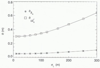
Fig. 5. Standard deviations of ![]() and
and ![]() for 250 estimates as a function of tie-point noise, σ, for
for 250 estimates as a function of tie-point noise, σ, for ![]() = 10 m, σBn = 0 m,
= 10 m, σBn = 0 m, ![]() , σBp = 0 m, Dy = 86.9 km, Dx = 85.8 km, σϕ = π/3 rad and Lx = 303.2 km.
, σBp = 0 m, Dy = 86.9 km, Dx = 85.8 km, σϕ = π/3 rad and Lx = 303.2 km.
Velocity error
In this subsection we examine the velocity error due to baseline inaccuracy for two typical situations that are likely to arise in the interferometric estimation of ice velocity. First we consider baselines estimated using stationary tie points on areas of bedrock near the ice-sheet margin. In this case it is important to understand how far onto the ice sheet the baseline estimate can be extended while maintaining reasonable accuracy for the velocity estimate. Secondly, baselines are determined using non-stationary tie points from areas on the ice sheet where there is little or no exposed bedrock to provide stationary points. In this situation it is important to understand how to select tie points to achieve sufficiently accurate velocity estimates with minimum field effort.
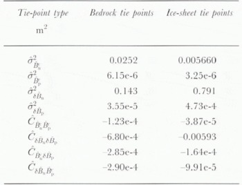
We begin using simulated bedrock tie points for a typical set of constraints. The parameters for the simulation are listed in Table 1. DEMs available for areas near ice-sheet margins typically have low horizontal and vertical resolution. Error in locating tie points in areas of an image where there are steep slopes increases the effective tie-point error. For these reasons we assume a relatively large tie-point error of σz = 100 m. Since it is easy to obtain a large number of tie points from a DEM, we use 100 tie points distributed uniformly over a 50km by 50km area. With sufficient averaging, phase noise can be kept low (Reference Li, and Goldstein,Li and Goldstein. 1990). For the simulation we use σϕ = π/20.
Table 1. Parameters for simulations with ice-sheet and bedrock tie points

The sample variance and covariance of 250 baseline estimates determined from bedrock tie points are given in Table 2. A contour plot of ![]() is given in Figure 6a. Since we are interested in using bedrock areas at the ice margin, the tie points are centered at x – x
c = –125 km, with the edge of the ice sheet at x – x
c = –100 km. Although the baselines were estimated for Lx
= 303.2 km, there is no reason velocity error cannot be computed for |x – x
c| > Lx
. In this figure the error is plotted out to a distance of 500 km inland from the ice-sheet margin (x – x
c = 400 km).
is given in Figure 6a. Since we are interested in using bedrock areas at the ice margin, the tie points are centered at x – x
c = –125 km, with the edge of the ice sheet at x – x
c = –100 km. Although the baselines were estimated for Lx
= 303.2 km, there is no reason velocity error cannot be computed for |x – x
c| > Lx
. In this figure the error is plotted out to a distance of 500 km inland from the ice-sheet margin (x – x
c = 400 km).

Table 2. Moments of baseline estimates from simulations with ice-sheet and bedrock tie points.
From Figure 6a we see that velocity error is smallest in the area near the tie points, and becomes steadily worse with increasing distance inland. Looking at the variation across the image, we see that accuracy is best at the center and worst toward the edges. At 200 km (x – x c = 100 km) inland the absolute error is >5 m year−1 with a relative error across the image of approximately 8 m year−1. The absolute error at 500 km from the ice-sheet margin is just over 12 m year−1, and the relative error is about 18 m year−1, which for many applications is unacceptably large.
Bedrock area is limited and in many cases smaller than in this example. Thus, increasing the bedrock area from which tie points are chosen is often not an option. Because there is little phase noise to begin with, its reduction will achieve only minor improvement. The baseline is short, so there is little to be gained by using an even smaller baseline. Furthermore, there are often only a limited number of baselines to choose from. In such cases, decreasing the baseline length may not be an option. Minor improvement may be achieved by increasing the number of tie points, but only so long as the tie-point errors remain uncorrelated. Because tie-point errors are large, the most significant improvement can be realized by decreasing tie-point error. For example, if tie-point error is reduced to 25 m. then velocity error decreases by a factor of about 3. Lesser gains are realized by a further decrease in tie-point error because phase noise begins to dominate.
Next we examine the case where velocity tie points measured on the ice sheet are used. The parameters for a typical set of ice-sheet tie points are given in Table 1. Because it is difficult to make such measurements, the minimum of four tie points is assumed. If tie-point velocity is measured over the period of a few weeks using GPS receivers, the error should be small. A high estimate of the velocity tie-point error is 0.8 m year−1. This error is included in the simulation by modeling it as an equivalent phase error of σϕ = π/5 rad. An additional phase error of σϕ = 3π/20 rad due to decorrelation yields a total phase error of σϕ = π/4 rad. Allowing for errors in locating the tie points within the SAR imagery, we assume elevation error of σz = 1 m. The tie points are arranged to form a square with 50 km sides centered about xe . The moments of the baseline estimates determined from this simulation are included in Table 2, and the corresponding velocity error is shown in Figure 6b.
Baseline estimates for ice-sheet tie points are not as accurate as those for bedrock tie points, making the velocity error larger. Even though the elevation error is much smaller, baseline accuracy is reduced because fewer tie points are used. Since the elevation error is small, no real improvement can be gained by improving the elevation estimates. Increasing the number of tie points would help, but the additional held effort may outweigh the gain. Tie-point velocity error also contributes to the larger velocity errors. Since a large estimate of tie-point Velocity error was used, significant improvement is possible if tie-point velocities are measured more accurately. If logistical constraints permit, increasing the separation of tie points will achieve much-improved results. For example, if the distances between tie points are increased to Dy = 100 km and Dx = 300 km, the velocity error decreases by a factor of about 8 to yield a maximum absolute error of just over 2 m for the entire 100 km by 500 km area. Thus, for tie points on the ice sheet, maximizing the spacing between points appears to be the best method for improving velocity estimates.
The results presented thus far have assumed a 3 d separation (δT = 3 d) for interferograms. Tie-point elevation error leads to error in the estimated velocity field, which is inversely proportional to δT. For bedrock tie points in particular, it is often possible to improve velocity estimates by using a longer temporal baseline. This situation is more complicated for non-stationary tie points. Error that is the result of error in the tie-point velocity measurements is independent of δT, so it does not decrease when δТ is increased. Thus, little is gained by using a longer temporal baseline if tie-point velocity error is the dominant source of baseline error.
Strain, melting and other surface changes cause temporal decorrelation to increase with time, placing an upper limit on δT. In the winter when there is no melting, temporal decorrelation is generally highest in regions with large strain rates. Therefore, longer temporal baselines are better suited for use in areas of slow-moving ice.
It is important to note that the preceding analysis is based on the assumption that the baseline varies linearly along track. Although we have obtained good results applying this assumption over distances of a few hundred kilometers, non-linear variation may have an effect over greater distances. If such variations occur, then more than four tie points are required either to fit the baseline variation to a higher-order polynomial or to use a piece-wise linear approximation.
Estimation of the Across-track Velocity Field
The displacement measured by an interferometric SAR is directed toward or away from the radar, but an estimate of the horizontal velocity is desired. Applying Equation (6), the horizontal velocity is related to the phase due to displacement by
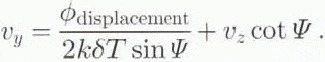
A simple approach to estimating horizontal velocity is to ignore the vertical-velocity term in the equation. Reference Joughin,, Winebrenner, and Fahnestock.Joughin and others (1995) have shown that while vertical velocity is small in comparison with horizontal velocity, vz is responsible for much of the phase variability over length scales of less than a few ice thicknesses. These fluctuations present little problem in determining the velocity field averaged over a few ice thicknesses. The error induced by neglecting vertical motion is far more significant, however, when examining horizontal-velocity variation over length scales comparable to the ice thickness. In particular, estimates of the local strain rate are severely affected by velocity error due to uncompensated vertical motion. As a result, it is often necessary to correct for the effect of vertical velocity when estimating horizontal velocity.
If we assume surface parallel flow, then the vertical velocity is related to the horizontal velocity by

Substituting this expression into Equation (21) yields.
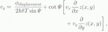
which is solved to yield
With this expression we now need the other horizontal velocity component, vx to determine vy . If we had another interferogram from a second look direction (i.e., an ascending pass), we could derive a similar expression relating vy to vx . With these two equations and Equation (22), the three components of the velocity field could be determined. Below we discuss a case where there are no interferograms from a second look direction.
Velocity Field for Humboldt Glacier
Humboldt Glacier is an outlet glacier in northwestern Greenland that discharges into the Kane Basin, Figure 7 shows an ERS-1 SAR amplitude image of the lower part of the Humboldt. The location of the image is shown on the map in Figure 8. The darker areas on the ice sheet along the bright calving face are bare ice in the ablation area. Fhe transition from this region to the adjacent brighter region marks the border of the wet-snow zone (Reference Fahnestock, Bindschadler,, Kwok and JezekFahnestock and others, 1993). The brighter areas in the lower corners of the image are within the percolation zone. Several lakes are visible, which show up as small bright circular regions in this winter imagery.
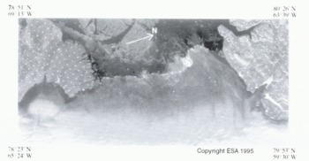
Fig. 7. SAR amplitude image of Humboldt Glacier, acquired 7 February 1992. The dimensions of the image are approximately 91 km across by 210 km long. The white squares indicate the locations of tie points used to estimate the baseline.
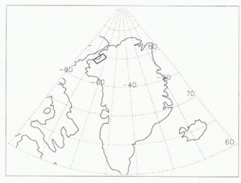
Fig. 8. Map of Greenland showing the location of SAR image containing the terminus of Humboldt Glacier.
We obtained SAR data from orbits 2904, 2947 and 2990, which spanned the interval 4–10 February 1992. The UK-PAF (United Kingdom Processing and Archiving Facility) SAR processor produces single-look, complex images with phase discontinuities. To circumvent this problem, we ordered raw SAR data and processed it ourselves to obtain single-look, complex images. Processing the data ourselves also allowed us to process successive 100 km by 100 km frames with the same Doppler parameters to eliminate phase discontinuities at frame boundaries.
Using the three images, we formed two 3 d interferograms with the image from Orbit 2947 common to both. The baseline for the 2904/2947 interferogram is approximately 236 m, and for the 2947/2990 interferogram approximately −10 m. These interferograms have streak errors similar to those observed by Reference Rignot,, Jezek, and Sohn,Rignot and others (1994) and Reference Joughin,Joughin (1995), although they are much less severe and not a significant source of error. The interferograms also have long spatial-wavelength (50–100 km) phase errors in the along-track direction that art-similar to those observed in interferograms of an area north of Jakobshavns Isbræ (Reference Joughin,Joughin, 1995). The long-wavelength errors in the Humboldt interferograms, however, are much smaller than those observed previously and have peak amplitudes of about 1 rad. The causes of the streak and long-wavelength errors are still unknown.
To cancel the effect of motion, we differenced the interferograms to yield a topography-only interferograms with an effective baseline of −246 m (Reference Joughin,, Winebrenner,, Fahnestoce,, Kwok and KrabillJoughin and Others, 1996). This interferogram was used in create a DFM for the area on the ice sheet. Figure 9 shows this DEM as a shaded surface overlaid with 100 m contours. In the bedrock areas phase gradients caused by steep slopes made it difficult to unwrap the phase. This problem could be eased by using a shorter baseline. We are primarily interested in the ice sheet, however, so we chose a longer baseline to achieve better accuracy and did not attempt to determine the bedrock topography. The bedrock elevations in Figure 9 are extracted from the same DEM that we used for tie-point information, which was provided by S. Ekholm (personal communication, 1994) of KMS (National Survey and Cadastre). There was too much decorrelation to unwrap the phase for a narrow band along the calving face. This part of the DEM has been filled in with elevation data from the KMS DEM. The lower resolution of the KMS data causes this area to appear smoother than adjacent regions in the shaded surface representation.
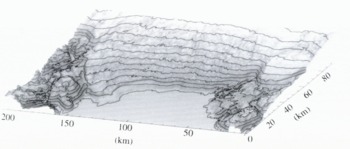
Fig. 9. Interferometrically derived DEM of the lower part of Humboldt Glacier. Bedrock elevations were determined photogrammetrically (personal communiction from S. Ekholm, 1994). The contour interval is 100 m. Illumination is directed from overhead along the vertical axis.
Ice-sheet elevations north of Jakobshavns Isbræ have been measured with 4 m absolute and 2.5 m relative accuracy (Reference Joughin,, Winebrenner,, Fahnestoce,, Kwok and KrabillJoughin and Others, 1996). DEM accuracy is largely determined by the quality of the tie points used to estimate the baseline. We are unlikely to have achieved accuracy this high since the Humboldt scene is near the coast, where altimetry-derived tie points on the ice sheet are most in error. These tie-point errors may cause our DEM to have a systematic error in the form of along- and a cross-track tilts that could yield errors of up lo several tens of meters. We hope to determine the accuracy of this DEM using laser altimeter data from the NASA Arctic ice-mapping lidar when it becomes available. We will also be able to improve the accuracy of the DEM using laser-altimeter tie points for the baseline estimate. Our current need for the DEM is to compute surface slopes to estimate velocity using Equation (24). Our DEM is well suited for this purpose since slope estimates are relatively unaffected by tie-point errors.
We used the 2947/2990 interferograin to estimate the across-track velocity field for Humboldt Glacier. Tie points from areas of bedrock (indicated by white dots in Figure 7) were used to estimate the baseline parameters: ![]() The baseline for this interferogram is much shorter than that of the topography-only interferogram, so regions consisting of bedrock were easily unwrapped. The effect of topography was removed using a synthetic interferogram created using the DEM. The result. ϕdisplacement, is shown in Figure 10. The phase is displayed rewrapped (i.e., modulo-2π) with irrelevant areas (sea ice) and areas that could not be unwrapped masked out.
The baseline for this interferogram is much shorter than that of the topography-only interferogram, so regions consisting of bedrock were easily unwrapped. The effect of topography was removed using a synthetic interferogram created using the DEM. The result. ϕdisplacement, is shown in Figure 10. The phase is displayed rewrapped (i.e., modulo-2π) with irrelevant areas (sea ice) and areas that could not be unwrapped masked out.
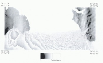
Fig. 10. Interferometric phase, ϕdisplacement, due to surface displacement in the radar look direction that occurred between 7 and 10 February 1992. Areas with no data correspond to regions where the phase could not be unwrapped or was masked (to avoid regions with sea ice).
We need to know the component of velocity in the along-track direction, vx , to estimate vy using Equation (24). We do not have an interferogram from a second look direction, so we have no direct knowledge of vx we knew the flow direction, then we could determine vx from vy . Flow direction can be estimated from the direction of maximum averaged downhill slope (Reference Paterson,Paterson, 1994). This yields an averaged How direction that misses perturbations in the direction of flow on scales less than a few ice thicknesses. Nevertheless, in the absence of other directional information this method may provide reasonable results.
In the Humboldt interferogram the across-track direction is nearly aligned with the direction of flow in most areas so that vx is small with respect to vy . Therefore, we neglect vx in our estimate of vy . This is simpler, and works almost as well as estimating flow direction from surface slopes. Since we are not estimating strain rates, the slightly larger error with this approach is insignificant.
Figure 11 shows estimates of vy
along a profile from the Humboldt data made with and without correction for vz
. Comparison of the profiles indicates that ignoring vz
leads to erroneous short-scale variability in the estimate, ![]() of up to 10 m year−1. This error is removed when the velocity is determined using Equation (24). The correction is imperfect fir this example because vx
is not known. Therefore, it is difficult to tell how much of the variability in the corrected profile is due to gradients in the horizontal velocity. This problem could be resolved with an interferogram from a second look direction.
of up to 10 m year−1. This error is removed when the velocity is determined using Equation (24). The correction is imperfect fir this example because vx
is not known. Therefore, it is difficult to tell how much of the variability in the corrected profile is due to gradients in the horizontal velocity. This problem could be resolved with an interferogram from a second look direction.
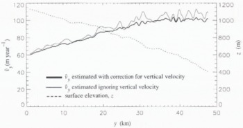
Fig. 11. Examples of horizontal velocity estimates made with and without correction for vertical velocity. Surface elevation is also shown.
Figure 12 shows the contours of the across-track velocity field for Humboldt Glacier. At slightly more than 100 km. Humboldt Glacier has the widest calving face of any outlet glacier in the Northern Hemisphere (Reference Weidick,Weidick and others, 1995). Reference Weidick,Weidick and others (1995) suspect that the calving face is grounded. In the SAR imagery (Fig. 7) it appears that most of the calving face is grounded, making this perhaps the longest continuous extent of grounded calving ice anywhere. Although its width makes it the broadest outlet glacier in Greenland, the velocity field for Humboldt Glacier (Fig. 7) reveals that the ice-flow speeds are moderate, and also that the enhanced speeds do not reach great distances inland. With ice-flow speeds of less than 100 m year −1 only 15 km from the calving front over the southwestern half of the glacier, it is clear that most of the discharge flux is carried in the northeastern half. Flow in this area exceeds speeds of 140 m year −1 25 km from the calving face, and produces a region of enhanced shear on the northeastern margin. This enhanced flow may be due to the presence of a channel in the bedrock.
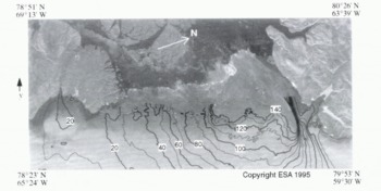
Fig. 12. Contours of across-track velocity, vy (m year −1). overlaid on SAR amplitude image.
We do not have independent estimates of ice velocity to directly evaluate the accuracy of our results. On the areas of bedrock, the velocity is zero, so we can estimate error for bedrock regions. After removal of topography, the mean of the phase in the bedrock area is −0.05 rad, and the standard deviation is 1.5 rad. This is equivalent to a velocity error with a mean of −0.07 m year −1 and a standard deviation of 2.1 in year−1.
In the previous section we estimated error due to baseline inaccuracy by means of simulation. In order to apply this procedure to the Humboldt area, we need to know the phase error and tie-point error. We do not have an accurate estimate of the error in the tie points extracted from the KMS DEM. Once the topographic effects arc removed, the phase variation in the bedrock area is the result of normal phase error and phase error due to uncompensated topography (DEM error). The standard deviation of the phase in this region is an estimate of the combined effects of phase and DEM error. Thus, when the standard deviation of the residual phase of the ice-free area is used in the simulation, the effect of tie-point elevation error does not have to be included explicitly as in the previous section.
The results of the simulation indicate that for the Humboldt scene the maximum standard deviation of the velocity error due to baseline error is ![]() year–1. Combining this error with the combined estimate of phase and DEM error from the ice-free areas (2.1 m year −1), the maximum velocity error on the ice-covered area is 2.3 m year−1. Actual errors may be slightly larger due to uncompensated vertical motion since vx
was ignored in applying Equation (24).
year–1. Combining this error with the combined estimate of phase and DEM error from the ice-free areas (2.1 m year −1), the maximum velocity error on the ice-covered area is 2.3 m year−1. Actual errors may be slightly larger due to uncompensated vertical motion since vx
was ignored in applying Equation (24).
In the prior simulations we assumed a low value (σϕ = π/20 rad) for the phase noise. After accounting for DEM error, the proportion of the 1.5 rad phase error attributable to phase noise due to speckle is larger ıhan expected (σϕ > 1 rad). Some, but not all, of this variation is caused by the long-wavelength phase errors described earlier (Reference Joughin,Joughin, 1995). The bedrock area in the upper righthand corner of Figure 10 has a mottled appearance, indicating some other source of error. Unlike speckle phase noise, which varies independently from pixel to pixel, this error has spatial structure over length scales of several kilometers. This cannot be uncompensated topography as the baseline is too short. Baseline errors would yield more linear tilt errors, Phase error with similar structure has been observed by Reference Goldstein,Goldstein (1995) for an area in the Mojavc Desert. California, U.S.A. He attributed it to additional time (phase) delay due to turbulent water vapor in the lower atmosphere. It is possible that the features in our data are the result of a similar phenomenon. It is interesting to note that the greatest anomalous phase variations are associated with area containing the most rugged topography. Further research is needed to resolve the exact cause and effect of these phase anomalies. Furthermore, because the error is spatially correlated it cannot be reduced by simple filtering, as with phase noise due to speckle.
Unmodeled Errors
The Humboldt interferograms and interferograms from other areas in Greenland (Reference Rignot,, Jezek, and Sohn,Rignot and others, 1994; Reference Joughin,, Winebrenner, and Fahnestock.Joughin. 1995) have streak errors, long-wavelength errors and errors that are likely due to atmospheric effects. None of these types of error was modelled in our simulations, because we do not yet have a good characterization of these errors. We do not even know the cause of streak and long-wavelength errors. These phase errors are a direct source of velocity error, and also contribute to it indirectly by causing larger baseline-estimation errors.
The long-wavelength error in particular is a problem when using tie points distributed over a small area. Consider the situation where tie points are dispersed over an area 25 km square. Assume a long-wavelength error that, over the tie-point area, varies linearly by 1 rad in the along-track direction. This would yield a baseline error of 10 rad or more when the baseline is extended 250 km inland. If the tie points were located at both ends of the 250 km area, long-wavelength errors would have only a minor effort on the baseline error. Al present, spreading out the tie points is the best way to overcome long-wavelength phase errors.
Further research is needed to understand the causes of these errors. We need to know their amplitudes and the frequency with which they occur. Once we understand the errors better, it may be possible to design algorithms to eliminate them. At the very least, we need to understand the errors well enough to determine their full impact on estimates of ice-flow velocity.
Conclusions
The results of the simulations suggest some rules that should be applied when choosing tie points. Four GPS-measured velocity tie points can provide good accuracy over large inland areas. The best way to improve accuracy with only four points is to maximize the spacing between points. Assuming elevation is known, geoloeation accuracy lot ERS-1/2 is of the order of 50 m (Reference Smity,, Wilson and Meadowns,Smith and others. 1994). Thus, tie points can be automatically geolocated within SAR imagery and need not be associated with any radar-visible features. There are few areas on the ice sheet where the strain rate or slope is so high that better determination of tie-point location is required. Tie points can easily be selected to avoid these areas. An interferogram with the shortest baseline available should be used to make velocity estimates.
For coastal areas, a reasonably detailed map (horizontal resolution of 0.5 km or better) and a sufficient area of exposed bedrock allow the baseline estimate to be extended onto the ice sheet with acceptable accuracy. The ability to use many tie points means that high accuracy is possible even with tie-point elevation errors on the order of 100 m for areas within 100–200 km of the coast. If large areas of bedrock are available, it is possible to extend the velocity estimates much further island with reasonable accuracy.
Our results have demonstrated that ice velocities accurate to within a few meters per year can be determined with SRI, although accuracy varies greatly with the quality of tie points. When both ascending and descending images are acquired during the tandem phase of ERS-1/2, it should be possible to map the full three-dimensional velocity field assuming surface parallel flow. The detailed velocity and topography information rendered by SRI provides an important new source of data for ice-sheet study.
Acknowledgements
I. Joughin and R. Kwok performed this work at the Jet Propulsion Laboratory. California Instilute of Technology, under contract with the National Aeronautics and Space Aflministration (NASA). M. Fahnestock was supported under NASA NMTPE grant NAGW4285.
We thank S. Ekholm of the National Survey and Cadastre, Copenhagen, Denmark, for providing us with the DEM. We also wish to thank C. Werner of the Jet Propulsion Laboratory for providing us with a SAR processor for the raw signal data. We would like to thank T. Scambos of the National Snow and Ice Data Center and the anonymous reviewer for their many helpful comments on the manuscript.


