

1. Introduction
Most of the Antarctic landscape consists of large snow-accumulation areas where surface melting is non-existent under current climatic conditions. However, in the near-coastal, blue-ice regions of Dronning Maud Land, below-surface ice-melt features have been regularly observed as part of recent Norwegian Antarctic. Research Expeditions (NARE) to the Jutulgryta area (Reference Winther, Elvehøy, Bøggild, Sand. and Liston.Winther and others, 1996). The melting phenomenon in Jutulgryta was first surveyed in February 1990, during NARE 1989–90, and later studied using a Land-sat Thematic Mapper (TM) image recorded on 12 February 1990 (Reference WintherWinther, 1993). The area was revisited for a period of 4 weeks during NARE 1993–94 (e.g. Reference Bøggild, Winther, Sand. and Elvehøy.Bøggild and others, 1995; Reference Winther, Elvehøy, Bøggild, Sand. and Liston.Winther and others, 1996), and revisited again for 5 weeks during NARE 1996–97. The study area is located at 71°24′S, 0°31′E, at approximately 150 m a.s.l. (Fig. 1). The large grain-sizes in the blue ice of this area suggest that it is old glacier ice that is reaching the surface due to a negative mass balance. As such, this blue ice and the associated melt features are similar to other Antarctic blue-ice areas located in coastal regions and around nunataks (Reference Van AutenboerVan Autenboer, 1962; Reference PaigePaige, 1968; Reference Orheim and Lucchitta.Orheim and Lucchitta, 1988; Reference Bintanja and van den Broeke.Bintanja and Van den Broeke, 1995b).
Location of the NARE study area in Jutulgryta, Dronning Maud Land, Antarctica.

The Jutulgryta area consists of gently rolling ice topography having ridge-to-valley distances of 1–4 km and ridge-to-valley heights of approximately 100 m. During winter, the region appears to experience strong and persistent easterly katabatic winds that generally keep the blue-ice surfaces swept free of winter snow accumulations (Reference Takahashi, Naruse., Nakawo. and Mae.Takahashi and others, 1988; Reference Van den Broeke and Bintanja.Van den Broeke and Bintanja, 1995a). These blue-ice areas have important physical characteristics that influence the local surface energy balance, meteorology and climate (Reference Bintanja and van den Broeke.Bintanja and Van den Broeke, 1995a, Reference Bintanja and van den Broeke.1996; Reference Van den Broeke and Bintanja.Van den Broeke and Bintanja, 1995b; Reference Bintanja, Jonsson. and Knap.Bintanja and others, 1997). The combination of easterly winds and rolling ice-surface topography leads to snowdrift-accumulation zones that form in the lee of the ice hills during winter. These snow-covered areas are found adjacent to the blue-ice fields in the form of bands 500–1000 m wide and several km long (Fig. 2). In Jutulgryta about 30% of the region is snow-covered.
Oblique image of snow and blue-ice patterns in Jutulgryta. Large snow stripe in foreground is approximately 500 m wide by 5 km long. Snow bands are oriented perpendicular to the easterly (from top-Left corner) katabatic winds.

The blue-ice areas of this region continually experience below-surface melting during the summer months; this generally occurs while the air and snow- and ice-surface temperatures are below freezing. The subsurface melting can be explained largely by the interactions between the snow/ice/water matrix and the near-surface radiation and energy balances. The low scattering coefficients that exist in the relatively large-grained blue ice allow shortwave solar radiation to penetrate the ice, thus providing a heat source below the ice surface that is sufficient to warm and melt the ice. Adjacent snow-accumulation areas have much higher scattering coefficients, and consequently limit solar-radiation penetration. The surface energy balance keeps both kinds of surfaces typically below freezing, and little surface melting occurs. In contrast to the below-surface meltwater produced in the blue-ice areas, below-surface melting in the nearby snow areas is minimal.
The meltwater produced by this mechanism drains within the blue-ice grain matrix and accumulates in lakes which drain both from distinct discharge channels and through the ice below. These meltwater-accumulation lakes can be a few km across (Reference Winther, Elvehøy, Bøggild, Sand. and Liston.Winther and others, 1996), and they lie upon ice that is approximately 500 m thick (personal communication from J. O. Näslund, 1997). Nearly all of the observed melting activity in the blue-ice areas occurs at least 15 cm below the typically frozen upper surfaces. Observed surface melting was generally confined to the base of penitents which formed facing the solar-noon sun (Reference LliboutryLliboutry, 1954; Reference Winther, Elvehøy, Bøggild, Sand. and Liston.Winther and others, 1996). Even the lakes, which in the summer months contain liquid water up to 1m deep, are covered by up to 10 cm of ice.
To help describe and explain the differences in melt-related features observed in the blue-ice and snow-covered areas of Jutulgryta, a physically based numerical model of the coupled atmosphere, radiation, snow and blue-ice system has been developed. The model comprises a heat-transfer equation that includes a spectrally dependent solar-radiation source term. The penetration of radiation into the snow and blue ice depends on the solar-radiation spectrum, the surface albedo and the snow and blue-ice grain-sizes and densities. In addition, the model uses a complete surface energy balance to define the upper snow and blue-ice surface boundary conditions. The model is run over the full annual cycle, simulating temperature profiles and melting and freezing quantities throughout the summer and winter seasons. The modeling system, and its validation, makes use of field observations collected during NARE 1996–97.
2. Model Description
The following physically based model has been formulated to describe the one-dimensional, time-dependent temperature and melting distributions within an ice sheet having characteristics which allow penetration of solar radiation into its upper layers. The formulation relies heavily on the methods of Reference SchlatterSchlatter (1972), who developed a model to study the subsurface temperature and melt profiles in Antarctica using a broad-band (spectrally independent and constant with depth) solar-radiation extinction coefficient. In addition, the current formulation makes strong use of the techniques developed by Reference Brandt and Warren.Brandt and Warren (1993), who modified Schlatter’s methodology to include the spectral dependence of solar radiation penetrating snow and ice. Reference Brandt and Warren.Brandt and Warren (1993) conclude that this spectral dependence is required to describe correctly the below-surface energy exchanges. In addition, they suggest that significant radiative heating differences can be expected under conditions of pure dense snow compared to conditions of blue ice.
a. General model equations
Energy is transferred through the snow/ice/water matrix by conduction along grain boundaries, and by vapor diffusion within pore spaces. In addition, this problem requires a solar-radiative energy source term that varies with depth. The general ice-temperature distribution and temporal evolution are described by the following one-dimensional heat-transfer equation,

where T i is the snow/ice temperature, z is the vertical coordinate, t is time, ρ i is the snow/ice density, C p is the specific heat of the snow/ice and q is the solar radiative f1ux. The thermal conductivity of the snow/ice matrix, k i (W m−1 K1), is given by Reference Sturm, Holmgren. and Morris.Sturm and others (1997):
where ρ i is in units of kg m−3. While Reference Sturm, Holmgren. and Morris.Sturm and others (1997) argue that this thermal conductivity generally includes the latent-heat transport across pore spaces due to vapor sublimation and condensation, they also demonstrate that there is a significant thermal-conductivity temperature dependence that is not represented by Equation (2). In order to include this temperature influence, the latent-heat flux coefficient, k v, is introduced that accounts for water-vapor diffusion within the air passageways, and is defined by

where L s is the latent heat of fusion, and R v is the gas constant for water vapor. The water-vapor diffusivity, D e (m2 s−1), is given by Reference AndersonAnderson (1976) as

and the saturation vapor pressure over ice, e si (Pa), is defined according to Reference MurrayMurray (1967),

where T i in Equations (4) and (5) is in K.
For the condition where meltwater is contained within the snow/ice matrix, k i is replaced with k iw, according to the formula
where f w is the water fraction, k w is the water thermal conductivity and k ice is the pure-ice thermal conductivity. A similar procedure is used for ρ i and C p in Equation (1).
b. Radiation penetration
The radiation flux penetrating the snow or ice, q, is computed using a two-stream approximation, as done by Reference SchlatterSchlatter (1972). In this formulation, when the downward solar flux, D, passes through a layer, dz, it is reduced by absorption and upward reflection, and enhanced by downward reflection of the upward flux U. Thus, the total change in downward flux is
where a and r are absorption and reflection coefficients, respectively. Using similar reasoning, the total change in upward flux is given by
Equations (7) and (8) have the boundary conditions D(0) = Q si and U (z 0) = 0, where Q si is the solar radiation reaching the surface, and z 0 is the depth at which solar radiation is no longer significant. The solution of Equations (7) and (8) follows the numerical scheme outlined in Schlatter (1972, appendix). The net solar radiative flux at level z within the snow/ice is given by
The coefficients a and r are dependent upon the surface albedo, α, and the attenuation rate of the downward solar flux, η(z), given by
Reference Brandt and Warren.Brandt and Warren (1993) define a downward bulk extinction coefficient corresponding to η(z),

where λ is the wavelength of the solar radiation, and Q λ is the incoming spectral solar flux at the surface. The spectral-flux extinction coefficient, η λ, in terms of the single-scattering co-albedo, (1 – ω), is given by
where ω is the single-scattering albedo, and g is an asymmetry factor. The extinction coefficient, σ c, is
where r i is the radius of a snow/ice grain, Q ext is the extinction efficiency, and the number of snow/ice grains per unit volume, N, is

where ρ ice is the density of pure ice.
c. Boundary conditions
The solution of Equation (1) requires top and bottom boundary conditions and initial conditions. The top boundary condition is determined by performing a full energy balance at the surface in the form
where Q si is the solar (shortwave) radiation reaching the surface of the earth, Q li is the incoming longwave radiation, Q lc is the emitted longwave radiation, Q h is the turbulent exchange of sensible heat, Q e is the turbulent exchange of latent heat, Q c is the conductive energy transport and Q m is the energy flux available for melt. Details of the formulation for each term in this energy balance are provided in the Appendix, where each term in Equation (15) is cast in a form that leaves the surface temperature, T 0, as the only unknown. Equation (15) is then solved for T 0, which is used as the top boundary condition for Equation (1). By making the model domain sufficiently deep to reproduce a temperature profile that is independent of depth and time in the lowest few meters of the domain over a full annual cycle, the bottom boundary condition is
where annual model integrations show this condition to be valid at z max = 15 m. For each of the simulations considered in this paper, initial conditions throughout the profile are given by imposing a constant profile equal to the mean annual air temperature, and then integrating the model, starting on 1 July, for 5 years using the same years’ atmospheric forcing data; at this stage the deepest ice temperatures have reached equilibrium. The model integration is continued for one additional year and the results are presented here. Equation (1), in conjunction with the boundary conditions defined by Equations (15) and (16), is solved using the finite control-volume methodology described by Reference PatankarPatankar (1980). For the model integrations presented in this paper, the grid interval over the 15 m vertical domain is fixed at 3 cm. Because atmospheric forcing data which resolve the diurnal cycle are not available, the model is run using a 1 day time-step. Inputs of observed daily-averaged surface meteorological data are used, and the daily-averaged incoming solar radiation is generated from computations of hourly values (see Appendix). We recognize that resolving the diurnal cycle would allow a better representation of the surface fluxes computed as part of the surface energy balance, and that the diurnal variation of solar radiation into the snow/ice matrix is an obvious feature of the natural system. However, given that the surface-temperature boundary condition is below freezing, the below-surface ice-melting problem generally reduces to a balance between the relatively-slow-time-scale conductive processes within the ice and the contributions of the solar-energy source term (Equation (1)). In our formulation, the total daily solar energy inputs into the snow/ice are the same whether the diurnal cycle is resolved or not. Since a primary aim of the current study is to resolve the seasonal cycle of below-surface meltwater production in snow and blue-ice areas (not the diurnal variations,, we have assumed that resolving the diurnal cycle in the model simulations is not required. As further justification for using this approach in the current study, in a previous study testing the validity of running ice-evolution models at daily time-steps, the lake-ice model of Reference Liston and Hall.Liston and Hall (1995) was used to show that simulations using an hourly time-step, with hourly data, produce results that are quite similar to simulations using daily averages of the hourly data, and running the model at a daily time-step.
d. Liquid-water treatment
As part of the model solution, the melting of ice and refreezing of water are handled by a water-fraction computation. Each model gridcell is assumed to have a water fraction and an ice fraction that sum to unity. Snow/ice temperatures computed above 0°C are reset to 0°C, and the temperature difference is used to determine the melt energy and resulting meltwater produced, expressed as a fraction of the gridcell. The temperature profile is then recomputed while forcing the 0°C temperatures to remain fixed. During the freeze-up of gridcells containing a non-zero water fraction, computed temperatures below 0°C are used to determine the “cold-energy” available to freeze the remaining liquid. Additional “cold-energy” available after the liquid fraction has been reduced to zero goes toward reducing the temperature below 0°C. This methodology conserves energy, while maintaining the condition that liquid water existing in the presence of ice cannot rise above 0°C. As part of the model formulation, the initially defined grain-size and density do not change during the simulated melting and refreezing processes, since it is assumed that such grain-evolution processes are secondary to the conduction and radiation influences simulated by the general heat-transfer equation. An additional model assumption is that, during a time-step, any water flowing into the uphill side of a gridcell is assumed to flow out of the downhill side. While we recognize this steady-state condition may not have held true during the entire annual cycle, it was typical of what was observed during the summer in the subsurface melting zone.
3. Model Inputs
To solve the above system of equations, additional information is required in the form of atmospheric forcing data, snow and blue-ice property data and the distributions of parameters describing the interaction between snow and ice grains and solar radiation. The distributions of Q ext, g and 1 – ω vary according to wavelength and snow/ice grain-size (Reference Wiscombe and Warren.Wiscombe and Warren 1980). Figure 3 provides distributions of these parameters for the range of grain-sizes of interest in this study; for grain radii greater than 2.5 mm, these distributions were extrapolated by computing the change in spacing between data distributions having radii less than 2.5 mm, and then extrapolating the spacing change to the larger grain-sizes. In addition, the downward solar-radiation spectrum reaching the surface, Q λ, must be known. The solar-radiation spectral distribution reaching the surface is defined by the Reference Stackhouse and Stephens.Stackhouse and Stephens (1991) two-stream, 256 spectral-band atmospheric radiation model for the case of a cloud-free atmosphere, a surface pressure of 980 mb and a solar zenith angle of 66°. The resulting distribution is given in Figure 4. During the snow-and ice-model simulations, Q λ is defined by scaling the distribution given in Figure 4, with the broad-band solar radiation reaching the surface, Q si. The computation of Q si is discussed in the Appendix as part of the surface-energy-balance formulation.
Distributions if the extinction efficiency, Qext, the single-scattering co-albedo, 1 – ω, and the asymmetry factor, g, as a function of wavelength and snow and ice grain-sizes (Wiscombe and Warren, 1980). Shown are values for grain radii, T, ranging from 0.5 to 10 mm, in steps of 0.5 mm. The 0.35 mm curves used in the model simulations (not shown) are similar to the 0.5 mm curves. (Data courtesy of S. G. Warren, University of Washington, Seattle.)

Downward solar spectrum reaching the surface, scaled by the broad-band (total) solar flux at the surface. Data generated using the Reference Stackhouse and Stephens.Stackhouse and Stephens (1991) model for a clear atmosphere, a surface pressure of 980 mb, and a solar zenith angle of 66°. (Data courtesy of J. Y. Harrington, Geophysical Institute, University of Alaska Fairbanks.)

Atmospheric forcing data required to complete the full annual integrations were obtained from the German Georg von Neumayer research station, located at 70°40′ S, 8°15′ W, at approximately 40 m a.s.l. (the Jutulgryta research site is approximately 85 km north of, 315 km east of and 110 m higher than the Neumayer station). A general comparison was made between 1994–95 data from this station and the limited meteorological data collected between 12 January and 9 February 1997 at the Jutulgryta research site, Neumayer was found to be moister and windier, and the average Neumayer air temperature was found to be within 1°C of the average Jutulgryta temperature during this 4 week summer period. Of particular importance to the current study is that both datasets suggest that summer air temperatures can be consistently ˂0°C. In spite of the difficulty in making such a comparison for different years, the Neumayer dataset has been assumed to be fairly representative of the conditions found in Jutulgryta, and the only adjustment made to the Neumayer data was to reduce the air temperatures by 1°C to account for the elevation difference. In light of its more coastal location and distance from the Jutulgryta site, the use of atmospheric forcing data from Neumayer is a significant approximation; unfortunately, no other suitable dataset is available. The 365 day, daily-averaged screen-height air temperature, relative humidity, atmospheric pressure (not shown) and wind speed used to drive the model simulations are provided in Figure 5.
Daily atmospheric forcing used in the model simulations. Also shown are the mean and standard deviation (s.d.). Data collected at the German Neumayer Antarctic research station, and made available as part of the World Meteorological Organization (WMO) World Weather Watch Program (http://www.ncdc.noaa.gov).

To solve the surface energy balance, the cloud-cover fraction is also required as input. Since this was unknown, it was used as a parameter that could be modified to vary the amount of incoming solar and longwave radiation reaching the snow/ice surface. In the simulations discussed herein a temporally constant cloud fraction of 0.54 was used. Comparisons of the monthly-mean, model-simulated incoming shortwave and longwave radiation with that observed at the Neumayer station in 1994–95 are found in Figure 6. While we recognize that the constant-cloud-cover-fraction assumption deviates from reality, Figure 6 suggests that, for the purposes of this study addressing processes assumed to be forced most strongly by the seasonal cycle, this assumption is acceptable.
Comparison of the monthly-mean, model-simulated incoming shortwave and longwave radiation, with that observed at the Mumayer station. (Data courtesy of the Alfred-Wegener-Institut, Germany.)

Snow- and ice-property data are also required by the model. Field observations during NARE 1996–97 are used to supply this information. The spectrally integrated albedo was obtained from a combination of observations using broad-band solar pyranometers and a portable spectroradimeter (252 hands, 370–1110 nm). These instruments were used over both snow and blue-ice areas, yielding representative albedos for each. Density and grain radii were measured as part of snow- and ice-pit excavations and analyses. Densities were measured with fixed-volume snow tubes (522 cm3) and a spring balance. An example observed snow-density profile is provided in Figure 7. The average observed blue-ice density of 800 kg m−3 was 50 kg m−3 lower than the Antarctic blue-ice density measured by Reference Bintanja and van den Broeke.Bintanja and Van den Broeke (1995b). The snow and blue-ice grain-sizes were measured by placing the grains on a mm grid board and viewing them with a hand lens. These observed property values are used in the model integrations and summarized in Table 1. In the natural system, the albedo and roughness differences between the snow and blue-ice surfaces are expected to lead to slightly different temperature and humidity conditions in the atmospheric boundary layer above the two surfaces. These differences, and the associated local heat and moisture advection, are largely unknown and assumed to be negligible in the current study. Applying different values of density, grain radii and albedo for snow and blue ice is the only difference between the two model simulations presented in this paper.
Example pit excavation displaying the vertical distribution of density and ice lenses in the snow areas. The observed ice-lens thicknesses and vertical positions are shown, and the density markers are data collected at 10 cm intervals.

Snow-and ice-property data used in the model simulations

Inputs of density and grain radii for snow and blue ice allow computation of the wavelength-dependent, spectral flux extinction coefficient given by Equation (12) (Fig. 8). Applying the solar-radiation spectrum given in Figure 4 allows computation of the downward bulk extinction coefficient variation with depth, η(z), for the properties of snow and blue ice (Fig. 9). This bulk extinction coefficient can be combined with the surface albedo to compute the absorption and reflection coefficients given by Equation (10), thus leading to a description of the solar-flux variation with depth within the snow and blue ice (Fig. 10). Also shown in Figure 10 are field observations of the solar flux, collected at 25 cm depth within the snow and blue ice. These observations were collected by digging a snow/ice pit, excavating laterally into the pit wall and placing an upward-oriented broad-band solar pyranometer at the roof of the lateral excavation. The pit was then filled in with the debris from the excavation. Because of the disturbed snow/ice below the sensor, this method modifies the radiation transport from below, and thus modifies the backscattered radiation above the sensor. To correct the sensor reading to simulate undisturbed below-sensor conditions, the two-stream radiative-transfer model was run for the conditions of disturbed snow/ice below the sensor (lower density and albedo), and the resulting simulations, when compared to the undisturbed simulations, were used to scale the observed radiation at 25 cm to correspond to the undisturbed conditions simulated by the model. While we recognize that this correction of the observations, by using the same model which we are comparing the observations to, has important deficiencies, the observations are still of sufficient quality to highlight the strong differences in solar-radiation extinction for snow and blue ice suggested by the model; these differences would still be valid without the corrections, although the magnitude of the values would he incorrect.
Wavelength-dependent spectral-flux extinction coefficient, ηλ, given by Equation (12), for snow and blue ice. The bottom display provides an expanded view of the shorter wavelengths given in the top display.

Depth variation of the downward bulk extinction coefficient, η(z),given by Equation (11), for snow and blue ice.

Net solar-flux variation with depth within snow and blue ice, non-dimensonalized by the broad-band (total) solar flux penetrating the surface. Also shown (solid dots) are field observations of solar flux, collected at 0.25 m depth, within the snow and blue ice.

The surface energy balance is coupled to the snow/ice below through the conduction term in Equation (15). Thus, solution of the snow/ice heat-transfer (Equation (1)) along with the surface energy balance yields a value for each term in Equation (15). The annual mean surface-energy-balance components for the snow and blue-ice simulations are given in Table 2. The dominant contribution to the surface energy balance is the net shortwave radiation. Figure 6 shows the appropriateness of the model simulation for both incoming shortwave and longwave radiation. As an additional comparison, Reference King and Connolley.King and Connolley (1997) list Neumayer annual mean climatologies, for incoming shortwave and longwave radiation, of 116.7 and 218.6 W m−2, respectively. Due to the differences in albedo, the blue-ice surface has greater net shortwave radiation at the surface. Averaged over the annual cycle, the surface temperature is slightly higher over blue ice than snow, leading to slightly greater emitted longwave radiation. The Table 2 values of emitted longwave radiation compare well with the 243.7 W m2 observed Neumayer climatology given by Reference King and Connolley.King and Connolley (1997). The resulting net radiation is positive for both surfaces, in contrast to the higher-latitude (74°34′S) and lower-albedo (0.55) blue-ice study of Reference Bintanja, Jonsson. and Knap.Bintanja and others (1997), who found a negative (–6.9 W m2) annual radiation balance. The latent-heat flux is strongly negative, and of a magnitude which suggests this study would benefit from annual ablation measurements. The surface conductive-heat flux is towards the surface, with larger values for blue ice, in response to the relatively high ice temperatures below.
Annual mean surface-energy-balance components from snow and blue-ice computations (positive values indicate transport towards the surface)

4. Computational Results
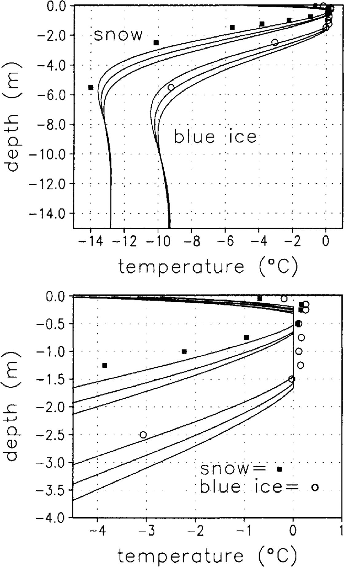
Solution of the general heat-transfer equation, after including the solar-radiation source term, produces temperature and water-fraction distributions within the snow and blue-ice media. The resulting temperature profiles far the snow and blue ice are given in Figure 11, where the solid lines represent July–January temperature profiles, and the dashed lines represent February–June profiles; both are plotted at 30 day intervals. These profiles are taken from the final year of a 6 year model integration, where the same annual atmospheric forcing has been applied during all 6 years. As a consequence, the zero-flux lower boundary condition has allowed the simulations to come to equilibrium with the surface forcing conditions, the internal thermal characteristics and the solar penetration. Evidently, the blue ice has an approximately 3.5°C higher deep-level temperature than the snow, and the entire blue-ice profile is generally warmer than the snow profile. During the warmest period, the snow-has a relatively small isothermal (0°C) region from 20 to 70 cm, while the blue ice has an isothermal region from 20 to 190 cm. The warm-season temperature profiles in Figure 11 correspond very well with the temperatures measured in the Jutulgryta area during NARE 1996–97. Figure 12 shows mid-January snow and blue-ice temperature observations (markers) along with simulated temperature profiles, where the modeled profiles are for the 20 day period (plotted at 10 day-intervals) around the observations. A range of modeled profiles is presented because the model is not simulating the same year as the observations. The below-surface temperature observations were collected using a vertical profile of geometrically spaced temperature sensors. The sensors were connected to a data logger and sampled hourly. Like other researchers (e.g. Reference Brandt and Warren.Brandt and Warren, 1993; Reference Bøggild, Winther, Sand. and Elvehøy.Bøggild and others, 1995), we had problems with radiative heating of our below-surface temperature sensors. To minimize the impact of this heating, the sensors were covered with a reflective foil, and the data presented in Figure 12 are collected from nighttime observations when solar heating was at a minimum. As seen in Figure 12, our sensors still read as high as +0.3°C in the upper levels of the snow/ice. The general character of the simulations compares well with the observations. While we recognize that adjustments to the snow grain-size and/or thermal diffusion coefficients could be made to produce an improved fit for the snow data, such an exercise seems unwarranted in light of the uncertainties with the observational datasets. These observed temperature profiles are similar to those measured by Reference Bøggild, Winther, Sand. and Elvehøy.Bøggild and others (1995) in this area in 1993–94.
Model-simulated temperature profiles for the snow (a) and blue ice (b). Solid lines represent temperature profiles from July–January, and dashed lines profiles from February–June; both are plotted at 30 day intervals.

Simulated (solid lines) and observed (markers) snow and blue-ice temperature profiles. Observations are from mid-January, and simulated profiles are plotted at 10 day intervals around that time. The bottom display is an expanded view of the upper profiles given in the top display.
The modeled summer temperature difference between the surface and the below-surface maximum for both snow and blue ice is 3–4°C (Fig. 12). This temperature difference is significantly greater than the 0.2°C reported by Reference Brandt and Warren.Brandt arid Warren (1993). The difference is, in part, the result of grain-size differences between their simulations and ours; they used a grain radius of 0.1 mm, which introduces much higher scattering influences than the relatively large grains considered in our study. There are other important differences between the simulations, two of which relate to the thermal diffusion coefficients used by the two different models. The latent-heat flux coefficient (Equation (3)) has a strong temperature dependence, and while the simulations presented in this paper include periods quite close to the freezing temperature, the simulations presented by Reference Brandt and Warren.Brandt and Warren (1993) consider temperatures between –28° and –20°C. In addition, the thermal conductivity used in our model (Equation (2)) leads to lower values than those used by Reference Brandt and Warren.Brandt and Warren (1993). The solution of the general heat equation accounts for influences from both solar radiation and heat conduction, and any modification of the thermal diffusion coefficients will lead to changes in heat-transfer rates within the snow/ice, and thus changes in the simulated temperature profiles. Reference Brandt and Warren.Brandt and Warren (1993) also consider the steady-state conditions achieved after 10 days of model integration time, while our runs are time-evolving. In addition, the surface and bottom boundary-condition formulations are different: they supply a surface flux, while we supply a surface temperature based on the surface fluxes, and they fix the lower boundary temperature, while we impose a zero-gradient lower boundary condition. There are also differences in the solar spectrum used in the simulations: theirs is computed for an atmospheric pressure of 680 mb, and ours is for 980 mb (thus, our absorption “windows” are more pronounced). These differences lead to subtle variations in the outputs of the two models, making direct comparison difficult. Supplying our model with inputs more consistent with Reference Brandt and Warren.Brandt and Warren (1993) for the simulation of a cold, fine-grained polar snowpack (adjusting the air temperature, grain-size, density, albedo and thermal conductivity) produces 0.5–1.5°C differences between the surface and the below-surface maximum (the value depends on the week chosen to look at the profile), and we conclude that our findings are generally consistent with theirs.
As part of the model solution, the fraction of water contained within each computational gridcell is accounted for. Figure 13 shows the seasonal evolution of the water fraction for snow and blue ice, as a function of depth. The solid lines represent water-fraction profiles prior to 15 January, and the dashed lines represent profiles after 15 January; both are plotted at 10 day intervals. Highlighted in Figure 13 are both the early-season increase in liquid water and the late-season freeze-up of that water. As one would intuitively expect in this system, Figure 13b shows that prior to 15 January the largest meltwater fraction is in the upper part of the melting profile, because the ice below the melting profile is at a much lower temperature than the ice above (Fig. 11b). In contrast, after 15 January the largest meltwater fraction is in the lower part of the melting profile, because the ice above the melting profile is now at a much lower temperature than the ice below (Fig. 11b). Thus, early in the melt season most of the meltwater is produced high in the meltwater profile, and during freeze-up the meltwater freezes from the top down.
Seasonal evolution of water fraction for snow (a) and blue ice (b), as a Junction of depth. Solid lines represent water-fraction profiles prior to 15 January, and the dashed lines profiles after 15 January; both are plotted at 10 day intervals.

The blue-ice simulation shows a much greater meltwater production than that found in the snow. This is qualitatively consistent with our field observations. The snow simulation indicates some meltwater production at about 50 cm depth. This is also consistent with our snow-pit observations, where we regularly observed ice lenses several cm thick at about this depth (Fig. 7). These lenses were found to be continuous throughout the length of 15 m snow trenches, and our observations did not reveal evidence of meltwater percolation columns that would indicate meltwater transport from higher in the snowpack. Ice lenses occur frequently within the snowpack, but their depths are quite variable, with a first lens found at about 15 cm, and the next found at depths of 40–80 cm (Fig. 7). In light of these model results, we speculate that the first ice lens, about 15 cm from the surface, is produced by radiation-trapping surface irregularities in the form of penitents (Reference Winther, Elvehøy, Bøggild, Sand. and Liston.Winther and others, 1996) which are generally about 10–15 cm in height (not accounted for by the model). Reference LliboutryLliboutry (1954) suggests that this melting at the base of the penitents is a key factor in penitents formation. We also conclude that the second ice lens is an annual feature created in the snow-covered areas by the mechanisms simulated by the model. Also shown in Figure 7 are ice lenses at depths below the the 50 cm level. We assume these lenses are features from previous years, although we have no way to confirm this. Identifying annual layering is made even more difficult by not knowing the annual winter snow accumulation in the snow areas; in the blue-ice areas winter snow accumulation appears to be very close to zero.
We were unable, as part of our field observations, to quantify the water fraction in the blue-ice areas; any excavation in such an area would quickly fill with water. This presence of large quantities of within-ice meltwater was also documented by Reference Winther, Elvehøy, Bøggild, Sand. and Liston.Winther and others (1996). During NARE 1996 97, a subsurface ice-basin discharge channel was observed to be transporting an average of 11750 m3 d−1 of water out of the study area over the period 22 January 8 February 1997. In addition, water-transport tracer studies indicated within-blue-ice water movement over distances of a few hundred meters. Thus, there is plenty of evidence that meltwater was produced within the blue-ice areas. We do know that the water fraction was never great enough to reduce the structural integrity of the ice to the point that it would collapse under a person’s weight. Based on these observations, we assume that the maximum water fraction simulated by the model, approximately 25%, may be reasonable. We believe that this value probably represents an upper bound, since water fractions greater than this would likely reduce the ice strength beyond what we observed; nothing we observed suggests that fractions greater than this occur.
The temporal evolution of the total-column water thickness for blue ice is given in Figure 14a. The slope of this curve is the water flux, or the meltwater production (or meltwater freeze-up if the values are negative), over the year (Fig. 14b). Also shown in Figure 14b is the 15 day running mean of the water flux. This water flux can also be thought of as the meltwater volume produced per unit area. As an additional validation of the model-produced water traction, the ratio of the observed ice-channel discharge to the model-computed water flux gives a crude approximation of the meltwater-contributing area. Thus, Figure 14b yields a mean water flux over the “discharge-measurement period of around 0.1 cm d1. This, in combination with the average measured discharge, suggests a contributing area of approximately 12 km2. This value seems quite reasonable in light of our knowledge of the surrounding ice topography and our observations of below-surface water transport; our topographic datasets indicate that 100 km2 is too large because of topographic divides and ridge-crest crevasses, and our below-surface transport observations indicate that transport distances of > 1 km are likely, so 12 km2 appears to be the correct order of magnitude. Such an analysis would benefit from running the subsurface melt model in a distributed sense, accounting for slope and aspect relationships, and by developing methods to route the meltwater through the “watershed” and into the discharge channel.
(a) Temporal evolution of total-column water thickness for blue ice. (b) Water flux, or meltwater production (or meltwater freeze-up if values are negative), and 15 day running mean, for blue ice.

The annual simulated temperature evolutions in the top 2.5 m for snow and blue ice are found in Figure 15, which also includes the water fraction, plotted using contours ranging from 0.0 to 0.225 in intervals of 0.025. This figure shows the higher temperatures and increased water quantities in the blue ice, the duration and distribution of meltwater, and the penetration of surface temperature variations.
Simulated annual temperature evolutions (grey shades, °C) in the top 2.5m for snow (a) and blue ice (b). Also included is the water fraction, plotted using contours ranging from 0.0 to 0.225 in intervals of 0.025.

The current study has found the wavelength-dependent formulation for the bulk extinction coefficient to successfully reproduce observed subsurface melting in snow and blue ice. It is more usual to apply a constant bulk extinction coefficient, which represents a significant simplification of the wavelength-dependent formulation presented herein (e.g. Reference SchlatterSchlatter, 1972; Reference Bintanja and van den Broeke.Bintanja and Van den Broeke, 1995b). To test the added value of using the wavelength-dependent formulation for the bulk extinction coefficient (Equations (11–14)), the snow and blue-ice simulations were repeated while applying a constant bulk extinction coefficient (η(z) = constant) of 6.1 m−1 for snow, and 3.3 m−1 for blue ice. These values were chosen by adjusting the constant coefficients until the maximum water fraction (Fig. 16) approximately matched those given by the wavelength-dependent simulations (Fig. 13). While we could have chosen these values based on some other criterion, the general conclusions would have been similar. For blue ice, the melting depth simulated by the wavelength-dependent (Fig. 13) and constant-coefficient (Fig. 16) formulations is about 1.7 and l.1 m, respectively. Our observations suggest that the 1.7 m value is more realistic (Fig. 12). Associated with this melting-depth difference is a change in maximum meltwater thickness from approximately 20 cm (Fig. 14) to 12 cm (not shown), and a change in final freeze-up date from early-April (Fig. 14) to mid-March (not shown). In addition to its improved physical basis and improved results, a clear advantage of adopting the wavelength-dependent formulation is that the extinction coefficients are determined by three easily measurable quantities: grain-size, density and albedo. It is this feature that has allowed us to characterize the distinct differences in observed subsurface melting between the snow and blue-ice areas of Jutulgryta.
Seasonal evolution of water fraction for snow (a) and blue ice (b), as a function of depth, for the case of vertically constant bulk extinction coefficients. Solid lines represent water-fraction profiles prior to 15 January, and dashed lines profiles after 15 January; both are plotted at 10 day intervals.

5. Conclusions
A numerical energy-transfer model has been developed and used to simulate the differences in solar-radiation extinction profiles and below-surface melting between the snow and blue-ice areas of Jutulgryta. The model accounts for the variation of wavelength-dependent solar-radiation interactions with snow and ice of varying grain-sizes and densities. This formulation allows the basic and readily observed snow and ice characteristics of surface albedo, grain-size and density to be used as model inputs, leading to a description of the penetration of solar radiation within the snow or ice. By simply modifying these three parameters (Table 1), the model appears to capture the salient differences between the observed meltwater production within the snow and blue-ice areas of Jutulgryta; all other aspects of the simulations are identical.
While quite pleased with the model results, we recognize that its formulation and implementation required numerous simplifications of the natural system. For example, in contrast to the single values used to define the basic model parameters like density and grain-size, our field observations show a range in these values. The values chosen for the simulations are averages of these quantities. Other, less general, values extracted from our observations could also have been used in the simulations, all leading to similar qualitative conclusions, while likely differing in detail. In light of our limited validation observations, it is difficult to justify the use of values other than those presented in Table 1; these values are consistent with other published observations obtained under similar conditions. The basic model assumption that the snow or blue ice comprising the vertical column is of uniform grain-size and density also deviates from what is observed. In the natural system, there are higher-density ice lenses, surface hoar and spatial variations that are not accounted for in the model. In addition, our observations suggest that the snow areas are actually snow-covered only to a depth of a few to several meters, and below that depth is blue ice. As another example, the use of daily-averaged solar radiation reaching the surface, instead of, say, hourly values, is a crude approximation which we have adopted since higher-temporal-resolution atmospheric-forcing datasets are not available.
In spite of our model assumptions, our observations and model integrations indicate that, even under conditions of surface air temperatures consistently below freezing, snow and ice melting below the surface can occur. This is the result of a solar-radiation energy source present within the snow and blue ice. The grain-size determines the wavelength-dependent scattering properties, and the grain-size and density determine the number of individual scatterers. The albedo determines the energy available to interact with the subsurface snow and ice. While this study has not attempted to determine the extent to which this kind of blue-ice melt process may take place in other Antarctic areas, it does suggest that blue-ice areas having similar physical characteristics and climate may be susceptible to subsurface melting for the same reasons it occurs in Jutulgryta.
Acknowledgements
The authors would like to thank S. Warren for providing the tables summarizing the grain-size-dependent and wavelength-dependent values of extinction efficiency, asymmetry factor and single-scattering co-albedo. In addition, we thank J. Harrington for providing the solar-spectrum data-set. This work could not have been completed without their assistance. We also thank R. Brandt and M. van den Broeke for their insightful reviews of this paper. The participants in NARE 1996–97 are gratefully acknowledged for their role in making the field program a success. This is publication No. 153 of the Norwegian Antarctic Research Expeditions. This work was funded by the Norwegian Research Council.
Appendix Surface Energy Balance
To determine the surface-temperature boundary condition required to solve Equation (1), a complete energy balance, given by Equation (15), is computed at the surface. In what follows, each term in that energy balance is described. Energy transports towards the surface are defined as positive.
The solar radiation striking the Earth’s surface, including the influence of sloping terrain, Q si, is given by
under the assumption that the angle between the direct solar radiation and a
sloping surface is given by i, and that diffuse radiation
impinges upon an area corresponding to a horizontal surface. The solar
irradiance at the top of the atmosphere striking a surface normal to the solar
beam is given by S * (=1370 W
m−2) (Reference Kyle, Ardanuy. and Hurley.Kyle and others,
1985), and ![]() and
and
![]() are the direct
and diffuse, respectively, net sky transmissivities, or the fraction of solar
radiation that reaches the surface. The solar zenith angle, Z,
is
are the direct
and diffuse, respectively, net sky transmissivities, or the fraction of solar
radiation that reaches the surface. The solar zenith angle, Z,
is
where ø is latitude, τ is the hour angle measured from local solar noon and δ is the solar declination angle. It is approximated by

where ø T is the latitude of the Tropic of Cancer, d is the Julian Day, d T is the day of the summer solstice and d y is the average number of days in a year.
The angle i is given by (Reference PielkePielke, 1984)
and the terrain slope, β, is

where Z t is the topographic height, and x and y are the horizontal coordinates. The terrain slope azimuth, with south having zero azimuth, is given by

and the solar azimuth, μ, with south having zero azimuth, is

To account for the scattering, absorption and reflection of shortwave radiation by clouds, the solar radiation is scaled according to
for direct solar radiation, and
for diffuse solar radiation, where σ c represents the cloud-cover fraction, and θ is a constant defined as 1.2 to provide a best fit to the observed Neumayer incoming shortwave radiation (Fig. 6) (Reference Burridge and Gadd.Burridge and Gadd, 1974).
The presence of clouds is accounted for in the computation of downward longwave radiation, Q li, and is given by
where σ is the Stefan–Boltzmann constant, and T r is the reference-level air temperature. As shown in Figure 6, Equation (A10) correctly simulates the observed Neumayer monthly values of downward longwave radiation for the period considered. This formulation is similar to that determined by Reference König-Langlo and Augstein.König-Langlo and Augstein (1994), without the exponential dependence on cloudiness; attempts to use their formulation to match the Figure 6 observations required much higher cloud-cover fractions (0.85) than the ones used in this study (0.54), and that, in turn, produced a misrepresentation of the model-simulated incoming solar radiation (Fig. 6).
The longwave radiation emitted by the snow/ice surface, Q le, is computed under the assumption that snow emits as a grey body,
where T 0 is the snow/ice surface temperature, and εs is the surface emissivity, assumed to be 0.98.
The turbulent exchange of sensible and latent heat, Q h and Q e, respectively, is given by
,

where ζ is a non-dimensional stability function, and the atmospheric pressure, p r, is given by Neumayer station observations. D h and D e are exchange coefficients for sensible and latent heat, respectively,

where u T is the wind speed at reference height z T, and z 0 is the roughness length for momentum, assumed to be equal to 10−4m. In this application the heat and moisture roughness lengths are assumed to equal that of momentum. The stability function, ζ, is defined following the surface flux parameterization of Reference LouisLouis (1979). Under unstable atmospheric conditions (Ri ˂ 0), ζ modifies the turbulent fluxes through the formula

where η = 9.4, and

where ψ = 5.3. Under stable atmospheric conditions (Ri > 0),
where η * = η/2. The bulk Richardson number, Ri, is

where g is the gravitational acceleration, and the atmospheric temperature gradient is computed using the reference-level air temperature and the surface temperature. Because of the non-linear character of the stability correction, the use of daily means to compute the turbulent fluxes is expected to lead to errors in the flux calculations. We have assumed that some stability correction is still desirable, and that this approximation is consistent with the other approximations made within this modeling effort.
Heat conduction flux at the surface, Q c, is given by
where T i is the snow/ice temperature, and k i is the thermal conductivity of the snow/ice matrix. The required temperature profile is computed from the general heat equation for snow/ice (Equation (1)).
To solve the system of surface-energy-balance equations for the surface temperature, the equations are cast in the form f(T 0) = 0, and solved iteratively for T 0 using the Newton-Raphson method. In the presence of snow, surface temperatures T 0 > 0°C resulting from the surface energy balance indicate that some energy is available for melting, Q m. The amount of energy available is then computed by setting the surface temperature to 0°C and recomputing the surface energy balance. A similar procedure is adopted to compute the energy available to freeze, Q f, any liquid water which may be present at the surface.


