



1 INTRODUCTION
Multi-wavelength data of z ~ 6 quasars have shown to be fundamental to understand the properties of the high-redshift Universe both on cosmological ( ⩾ tens of Mpc) and galactic scales ( ⩽ tens of kpc). In the last two decades, more than 100 z ~ 6 quasars have been discovered through various different surveys. Initially, most of them were found at 5.7 ⩽ z ⩽ 6.4 with the SDSS and the CFHQS (e.g. Jiang et al. Reference Jiang2009, Willott et al. Reference Willott2010b and references therein). Nowadays, new surveys with enhanced sensitivities in the red and near-IR as Pan-STARRS1 (Bañados et al. Reference Bañados2016), VST/ATLAS (Carnall et al. Reference Carnall2015), DES (Reed et al. Reference Reed2015, Reference Reed2017), Subaru/HSC (Matsuoka et al. Reference Matsuoka2016), UKIDSS (Venemans et al. Reference Venemans2007), and VIKING (Venemans et al. Reference Venemans2013, Reference Venemans2015a) are discovering further quasars at similar and higher redshift. Currently, the highest redshift quasar known is ULASJ1120+0641, discovered in UKIDSS at z = 7.09 (Mortlock et al. Reference Mortlock2011) (Figure 1).
Spectrum of ULAS J1120+0641 (black line) compared to a composite spectrum derived from lower redshift quasars (red line, Telfer et al. Reference Telfer2002). Adapted from Figure 1 of Mortlock et al. (Reference Mortlock2011) by permission of the authors and the Nature Publishing Group; courtesy of Daniel Mortlock.

On large scales, observations of z ~ 6 quasars have been extensively used as powerful probes of the cosmic reionisation process. Optical/near-infrared absorption spectra of z ~ 6 quasars in the spectral region blue-ward the Lyα emission line are characterised by the presence of ionised near zones (2–12 physical Mpc, e.g. Fan et al. 2006; Venemans et al. Reference Venemans2015b; Reed et al. Reference Reed2017) interrupted by deep absorption gaps that extend up to hundreds of Mpc (Gallerani et al. Reference Gallerani2006; McGreer et al. Reference McGreer2015; Becker et al. Reference Becker2015). The sizes of quasar near zones are generally used to constrain the intergalactic medium (IGM) neutral hydrogen fraction (e.g. Mesinger & Haiman Reference Mesinger and Haiman2004; Maselli et al. Reference Maselli2007; Keating et al. Reference Keating2015). In particular, evidence for a Lyα damping wing has been found in ULASJ1120+0641 suggesting a neutral hydrogen fraction x
HI > 0.1 (Mortlock et al. Reference Mortlock2011). More recently, Greig et al. (Reference Greig2017a) have used the same observations to provide more stringent constraints on the neutral hydrogen fraction (x
HI = 0.4+0.21
−0.19) thanks to the Lyα emission line reconstruction method presented by Greig et al. (Reference Greig2017b). These studies on the IGM ionisation state are fundamental to constrain models of the cosmic reionisation process (e.g. Choudhury & Ferrara Reference Choudhury and Ferrara2005; Choudhury et al. Reference Choudhury2008; Mitra et al. Reference Mitra2012, Reference Mitra2016) to finally understand this important phase transition in the evolution of the Universe. Ionised regions around high-z quasars also provide measurements of the average IGM temperature at the mean density (T
0 = 104.21 ± 0.03K, Bolton et al. Reference Bolton2012), the quasar lifetimes ( $t_\text{Q}\sim 10^6\text{--}10^8 \rm yr$
, e.g Gallerani et al. Reference Gallerani2008) and the environment in which high-z quasars form and evolve (e.g. Kim et al. Reference Kim2009; Maselli et al. Reference Maselli2009).
$t_\text{Q}\sim 10^6\text{--}10^8 \rm yr$
, e.g Gallerani et al. Reference Gallerani2008) and the environment in which high-z quasars form and evolve (e.g. Kim et al. Reference Kim2009; Maselli et al. Reference Maselli2009).
On small scales, z ~ 6 quasars are ideal laboratories for studying the properties of the host galaxy and its coeval formation with the super-massive black holes (SMBHs) they contain. In the spectral region red-ward the Lyα emission line, the quasar continuum retains precious information on the dust properties of the host galaxy. It has been shown that extinction properties of high-z quasars are well described in terms of SN TypeII dust (e.g. Maiolino et al. 2004; Gallerani et al. Reference Gallerani2010), though this argument is still subject of hot debate. Moreover, while metal absorption lines can be used to study the global IGM metal enrichment (e.g. Pallottini et al. Reference Pallottini2014; D’Odorico et al. Reference D’Odorico2013; Oppenheimer et al. Reference Oppenheimer2012; Ryan-Weber et al. Reference Ryan-Weber2009), metal emission lines provide information on the metallicity of the quasar host galaxy (e.g. Fan et al. Reference Fan2004; Juarez et al. Reference Juarez2009). The inferred metallicity of the gas in the quasar broad line region (BLR) is super-solar, similarly to what is observed at lower redshifts. Moreover, Mgii emission line observations in the near-IR provide measurements of the mass of black holes powering z ~ 6 quasars (e.g. Willott et al. Reference Willott2003). These studies show that high-z quasar host galaxies contain SMBHs rapidly grown up to a mass $M_{\bullet }\ge 10^{9}\text{M}_{\odot }$
. The current most massive black hole (
$M_{\bullet }\ge 10^{9}\text{M}_{\odot }$
. The current most massive black hole ( $M_{\bullet }=1.24\; \pm\; 0.19 \times 10^{10}\text{M}_{\odot }$
) is powering a quasar at z = 6.3 (Wu et al. Reference Wu2015) (Figure 2). The presence of SMBHs formed in such a short time strongly challenges the standard black hole growth theory, as extensively discussed in Section 2. The detection of SMBH progenitors would be extremely important both to understand the formation of these massive systems (e.g. Pezzulli et al. Reference Pezzulli2016, Reference Pezzulli2017) and to clarify the contribution of faint quasars to the cosmic reionisation process (e.g. Volonteri & Gnedin Reference Volonteri and Gnedin2009; Giallongo et al. Reference Giallongo2015; Madau & Haardt 2015; Manti et al. Reference Manti2017; Kulkarni et al. Reference Kulkarni2017).
$M_{\bullet }=1.24\; \pm\; 0.19 \times 10^{10}\text{M}_{\odot }$
) is powering a quasar at z = 6.3 (Wu et al. Reference Wu2015) (Figure 2). The presence of SMBHs formed in such a short time strongly challenges the standard black hole growth theory, as extensively discussed in Section 2. The detection of SMBH progenitors would be extremely important both to understand the formation of these massive systems (e.g. Pezzulli et al. Reference Pezzulli2016, Reference Pezzulli2017) and to clarify the contribution of faint quasars to the cosmic reionisation process (e.g. Volonteri & Gnedin Reference Volonteri and Gnedin2009; Giallongo et al. Reference Giallongo2015; Madau & Haardt 2015; Manti et al. Reference Manti2017; Kulkarni et al. Reference Kulkarni2017).
Combined optical/near-infrared spectrum of J0100+2802. Based on the Mg ii Full Width at Half Maximum (FWHM = 5130±150kms−1), and the continuum luminosity at the rest-frame wavelength of 3000 Å (3.15±0.47 × 1047ergss−1), Wu et al. (Reference Wu2015) estimate a black hole mass $(1.24\;\pm\; 0.19) \times 10^{10}\,\text{M}_{\odot }$
for this source. Reproduced from Figure 3 of Wu et al. (Reference Wu2015) by permission of the authors and the Nature Publishing Group.
$(1.24\;\pm\; 0.19) \times 10^{10}\,\text{M}_{\odot }$
for this source. Reproduced from Figure 3 of Wu et al. (Reference Wu2015) by permission of the authors and the Nature Publishing Group.

More recently, radio, millimetre, and sub-millimetre observations (VLA, ALMA, and NOEMA) have provided a new window on ⩽ kpc scales to study the cold gas and dust physical condition in the interstellar medium (ISM) of z ~ 6 quasar host galaxies (see Carilli & Walter Reference Carilli and Walter2013 and references therein). These observations have been useful to characterise the properties of z ~ 6 quasar host galaxies (e.g. in terms of star formation rate (SFR), dust masses, dynamical mass, molecular hydrogen mass, feedback), to understand the co-evolution of galaxies and their SMBHs at high-z (e.g. Valiante et al. (Reference Valiante2017) for a recent theoretical review on this subject), and may provide new tools for detecting SMBH progenitors with important implications for the formation of these massive systems and for the contribution of faint quasars to cosmic reionisation.
In this review, we first discuss the latest results obtained from studies on the SMBH formation; then, we focus on the most recent millimetre and sub-millimetre observations of far infrared (FIR) emission lines arising from the ISM of z ~ 6 quasars; finally, we discuss possible observational strategies that could help us progressing in the comprehension of the first quasar physical properties.
2 THE FORMATION AND EVOLUTION OF SMBHs
Black hole mass estimates rely on the measurement of broad emission lines (BELs) widths, and are based on the assumption that the dynamics of the BLRs are dominated by the gravity of the central BH (see Peterson Reference Peterson2014). The black hole mass can thus be expressed as
 $$\begin{equation}
M_{\rm BH}\propto G^{-1}\,R_{\rm BLR}v_{\rm BLR}^2,
\end{equation}$$
$$\begin{equation}
M_{\rm BH}\propto G^{-1}\,R_{\rm BLR}v_{\rm BLR}^2,
\end{equation}$$
The maximum black hole masses found at high redshifts are comparable to the most massive objects found in the local Universe and to the theoretical maximum black hole mass achievable by luminous accretion ( ~ 1010M⊙, see Natarajan & Treister Reference Natarajan2009, King Reference King2016). The challenge is to understand how these SMBHs have formed in less than ~ 1 Gyr, the age of the Universe at z ~ 6 (e.g. Volonteri et al. Reference Volonteri2003; Volonteri Reference Volonteri2010).
In the standard growth scenario, the luminosity of an accreting black hole can be expressed through the following relation:
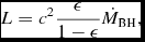 $$\begin{equation}
L=c^2\frac{\epsilon }{1-\epsilon }\dot{M}_{\rm BH},
\end{equation}$$
$$\begin{equation}
L=c^2\frac{\epsilon }{1-\epsilon }\dot{M}_{\rm BH},
\end{equation}$$ $\dot{M}_{\rm BH}$
is the black hole mass accretion rate (see Trakhtenbrot et al. Reference Trakhtenbrot2017a for a recent work on radiative efficiencies and accretion rates of z ~ 6 quasars). Under the assumption that the black hole is shining at the Eddington luminosity (
$\dot{M}_{\rm BH}$
is the black hole mass accretion rate (see Trakhtenbrot et al. Reference Trakhtenbrot2017a for a recent work on radiative efficiencies and accretion rates of z ~ 6 quasars). Under the assumption that the black hole is shining at the Eddington luminosity (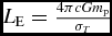 $L_\text{E} = \frac{4\pi cGm_\text{p}}{\sigma _T}$
), it grows in mass exponentially:
$L_\text{E} = \frac{4\pi cGm_\text{p}}{\sigma _T}$
), it grows in mass exponentially:
 $$\begin{equation}
M_{\rm BH}(t)=M_{\rm BH}(0)\,\rm exp\left(\frac{1-\epsilon }{\epsilon }\frac{\it t}{\it t_{\rm Edd}}\right),
\end{equation}$$
$$\begin{equation}
M_{\rm BH}(t)=M_{\rm BH}(0)\,\rm exp\left(\frac{1-\epsilon }{\epsilon }\frac{\it t}{\it t_{\rm Edd}}\right),
\end{equation}$$
Black hole seeds can either form small and grow fast (i.e. overshooting the Eddington limit), or form big and grow at a normal pace, at or below Eddington. In the first scenario, BH seeds are formed from the collapse of primordial (PopIII) stars, metal-free objects as massive as hundreds of solar mass and hosted in dark matter mini-halos ( $M_\text{h}\sim 10^{5-6}\,\text{M}_{\odot }$
) at z > 20 [e.g. Tegmark et al. Reference Tegmark1997; Abel et al. Reference Abel2002; see also Ciardi & Ferrara (Reference Ciardi and Ferrara2005) for a review on this topic]. BH remnants from PopIII stars are expected to be ⩽ 100M⊙ (e.g. Schneider et al. Reference Schneider2002; Zhang et al. Reference Zhang2008). Although this path to form a BH seed seems to be very natural, large uncertainties exist on the final mass of PopIII stars and only the most optimistic assumptions can explain the SMBH origin from PopIII remnants. The feasibility of this scenario could be improved by allowing accretion rates not to be limited to the Eddington rate (see Volonteri & Rees Reference Volonteri and Rees2005, Alexander & Natarajan Reference Alexander and Natarajan2014, Madau et al. Reference Madau2014, and Volonteri et al. Reference Volonteri2015). These works suggest that short and recurring episodes of super-Eddington accretion may take place, speeding up the growth process. This may occur in heavily buried seeds, in which photon trapping reduces the efficiency of radiation pressure. In the alternative scenario, black hole seeds are formed with heavy masses, from ~ 103M⊙ up to ~ 105M⊙. In this case, super-Eddington accretion would not be required. For instance, as soon as the gas is polluted by metals created in the first PopIII stars, the normal PopII star formation mode can proceed. This first episode of efficient star formation can foster the formation of very compact nuclear star clusters where star collisions can lead to the formation of a very massive star, possibly leaving BH remnants with masses ~ 103M⊙ (e.g. Devecchi & Volonteri Reference Devecchi and Volonteri2009 and Davies et al. Reference Davies2011). Even larger BH seeds may be achieved in the direct collapse black hole (DCBH) scenario, described in the following section.
$M_\text{h}\sim 10^{5-6}\,\text{M}_{\odot }$
) at z > 20 [e.g. Tegmark et al. Reference Tegmark1997; Abel et al. Reference Abel2002; see also Ciardi & Ferrara (Reference Ciardi and Ferrara2005) for a review on this topic]. BH remnants from PopIII stars are expected to be ⩽ 100M⊙ (e.g. Schneider et al. Reference Schneider2002; Zhang et al. Reference Zhang2008). Although this path to form a BH seed seems to be very natural, large uncertainties exist on the final mass of PopIII stars and only the most optimistic assumptions can explain the SMBH origin from PopIII remnants. The feasibility of this scenario could be improved by allowing accretion rates not to be limited to the Eddington rate (see Volonteri & Rees Reference Volonteri and Rees2005, Alexander & Natarajan Reference Alexander and Natarajan2014, Madau et al. Reference Madau2014, and Volonteri et al. Reference Volonteri2015). These works suggest that short and recurring episodes of super-Eddington accretion may take place, speeding up the growth process. This may occur in heavily buried seeds, in which photon trapping reduces the efficiency of radiation pressure. In the alternative scenario, black hole seeds are formed with heavy masses, from ~ 103M⊙ up to ~ 105M⊙. In this case, super-Eddington accretion would not be required. For instance, as soon as the gas is polluted by metals created in the first PopIII stars, the normal PopII star formation mode can proceed. This first episode of efficient star formation can foster the formation of very compact nuclear star clusters where star collisions can lead to the formation of a very massive star, possibly leaving BH remnants with masses ~ 103M⊙ (e.g. Devecchi & Volonteri Reference Devecchi and Volonteri2009 and Davies et al. Reference Davies2011). Even larger BH seeds may be achieved in the direct collapse black hole (DCBH) scenario, described in the following section.
2.1 Direct collapse black holes
In the early Universe, the collapse of a primordial atomic-cooling halo, exposed to a Lyman–Werner (LW, energy hν = 11.2–13.6eV) flux intense enough to efficiently dissociate molecular hydrogenFootnote 1 , may lead to the formation of a DCBH, through a general relativistic instability (Shang et al. Reference Shang2010; Johnson et al. Reference Johnson2012; Ferrara et al. Reference Ferrara2014). The rationale of these conditions is that the primordial gas needs to contract without cooling and fragmenting into stars. Then, the absence of the main coolants (metals and molecular hydrogen, dissociated by the LW radiation) may serve the purpose. The final result of this process is the formation of a BH seed having mass of the order of 104 − 106M⊙ (see the birth mass function for DCBHs presented in Ferrara et al. Reference Ferrara2014).
In recent years, the scientific community has focussed much attention on this scenario, likely due to the following reasons: (i) it is theoretically elegant and well tailored to the physical conditions of the early Universe, (ii) the (predicted) observational signatures of these objects are easier to check in actual observations, e.g. the absence of metal lines, and (iii) the predicted masses are sufficiently large to allow for their direct observation with current or upcoming surveys.
Much effort has been devoted recently in understanding the observational properties of these sources. For instance, Pacucci et al. (Reference Pacucci2015b) investigated the time-evolving spectrum of an accreting DCBH of initial mass M
• = 105M⊙ (Figure 3, left panel) by coupling a 1D radiation-hydrodynamic code (Pacucci & Ferrara Reference Pacucci and Ferrara2015) to the spectral synthesis code CLOUDY (Ferland et al. Reference Ferland2013). The DCBH is at the centre of a halo of total gas mass $M_{\text{g}} \simeq 10^7 {\rm M_\odot }$
, distributed in a core plus an r
−2 density profile. The accretion is followed until complete depletion of the halo gas, i.e. for ≃ 120Myr. During this period, the total absorbing column density of the gas varies from an initial value of ~ 1024cm−2 to a final value ≪ 1022cm−2, i.e. from being mildly Compton-thick to strongly Compton-thin. Note that while Lyα attenuation by the ISM is included, this work does not account for the likely sub-dominant IGM analogous effect. The bulk of the emission occurs in the observed infrared-submm (1–1000μm) and X-ray (0.1–100keV) bands. This work has recently been extended by Natarajan et al. (Reference Natarajan2017), with a more comprehensive study of the gas metallicity effects and seed formation mechanism on the emerging spectrum. Moreover, the first multi-wavelength spectral predictions for JWST observability of these sources were presented.
$M_{\text{g}} \simeq 10^7 {\rm M_\odot }$
, distributed in a core plus an r
−2 density profile. The accretion is followed until complete depletion of the halo gas, i.e. for ≃ 120Myr. During this period, the total absorbing column density of the gas varies from an initial value of ~ 1024cm−2 to a final value ≪ 1022cm−2, i.e. from being mildly Compton-thick to strongly Compton-thin. Note that while Lyα attenuation by the ISM is included, this work does not account for the likely sub-dominant IGM analogous effect. The bulk of the emission occurs in the observed infrared-submm (1–1000μm) and X-ray (0.1–100keV) bands. This work has recently been extended by Natarajan et al. (Reference Natarajan2017), with a more comprehensive study of the gas metallicity effects and seed formation mechanism on the emerging spectrum. Moreover, the first multi-wavelength spectral predictions for JWST observability of these sources were presented.
Left panel: Time evolution of the spectrum emerging from the host halo for a source located at z = 9, in the standard accretion case, with the density profile investigated in Pacucci et al. (Reference Pacucci2015a), i.e. with a core number density of 106 cm−3. The infrared, optical, and X-ray bands are highlighted with shaded regions, while the unprocessed spectrum is reported, at peak luminosity (t = 115Myr), with a dashed line. The flux limits for future (JWST, ATHENA) and current (CDF-S) surveys are also shown. The left panel is reproduced from Pacucci et al. (Reference Pacucci2015b). Upper right panel: Time evolution of the Lyα (blue solid line), He $\scriptstyle \rm II$
(red dashed line) line, and X-ray (violet dot dashed line) luminosities calculated for the accretion process onto a DCBH of initial mass 105M⊙. The green shaded region indicates the period of time during which the simulation results are compatible with CR7 observations. The current upper limit for X-ray is ≲ 1044ergs−1 (horizontal violet line, Elvis et al. Reference Elvis2009). Lower right panel: Time evolution of the
$\scriptstyle \rm II$
(red dashed line) line, and X-ray (violet dot dashed line) luminosities calculated for the accretion process onto a DCBH of initial mass 105M⊙. The green shaded region indicates the period of time during which the simulation results are compatible with CR7 observations. The current upper limit for X-ray is ≲ 1044ergs−1 (horizontal violet line, Elvis et al. Reference Elvis2009). Lower right panel: Time evolution of the ${\rm He\, }\text{\textsc {ii}}/{\rm Ly}\alpha$
lines ratio. The black horizontal dashed line indicates the observed values for CR7. The right panel is reproduced from Pallottini et al. (Reference Pallottini2015).
${\rm He\, }\text{\textsc {ii}}/{\rm Ly}\alpha$
lines ratio. The black horizontal dashed line indicates the observed values for CR7. The right panel is reproduced from Pallottini et al. (Reference Pallottini2015).

The DCBH template spectrum presented by Pacucci et al. (Reference Pacucci2015b) has been used to interpret observations of CR7 at z ≈ 6.6 (Sobral et al. Reference Sobral2015). This source is the brightest Lyα emitter discovered to date and shows some peculiar observational features, like strong Lyα and He ii emission lines and absence of metal lines. Though initially this source was identified as a possible PopIII galaxy, Pallottini et al. (Reference Pallottini2015) have discarded this hypothesis (unless under somehow extreme conditions; see also Yajima & Khochfar Reference Yajima and Khochfar2017 and Visbal et al. Reference Visbal2017) and suggested that this source most likely host a DCBH (see also Agarwal et al. Reference Agarwal2016; Dijkstra et al. Reference Dijkstra2016; Smith et al. Reference Smith2016). The right panel of Figure 3 shows the time evolution of the Lyα, He ii, and X-ray (0.5–2 keV) luminosities for a typical DCBH of initial mass ~ 105M⊙. Both Lyα and He $\scriptstyle \rm II$
are consistent with the observed CR7 values during an evolutionary phase lasting ≃ 17Myr (14% of the system lifetime).
$\scriptstyle \rm II$
are consistent with the observed CR7 values during an evolutionary phase lasting ≃ 17Myr (14% of the system lifetime).
The equivalent width of the He $\scriptstyle \rm II$
line in the CR7 compatibility region (green shaded region in the right panel of Figure 3) ranges from 75 to 85 Å. The column density during the CR7-compatible period is ≃ 1.7 × 1024cm−2, i.e. mildly Compton-thick. The associated X-ray luminosity is
$\scriptstyle \rm II$
line in the CR7 compatibility region (green shaded region in the right panel of Figure 3) ranges from 75 to 85 Å. The column density during the CR7-compatible period is ≃ 1.7 × 1024cm−2, i.e. mildly Compton-thick. The associated X-ray luminosity is $L_\text{X}\lesssim 10^{43}\,{\rm erg}\,{\rm s}^{-1}$
, fully consistent with the current upper limit for CR7 (
$L_\text{X}\lesssim 10^{43}\,{\rm erg}\,{\rm s}^{-1}$
, fully consistent with the current upper limit for CR7 ( $L_\text{X}\lesssim 10^{44}\,{\rm erg}\,{\rm s}^{-1}$
) obtained by Elvis et al. (Reference Elvis2009). Deeper X-ray observations of CR7 might then confirm the presence of the DCBH. However, this limit is already obtained with 180 ks of integration time on Chandra, meaning that a stringent test might only be possible with the next generation of X-ray telescopes.
$L_\text{X}\lesssim 10^{44}\,{\rm erg}\,{\rm s}^{-1}$
) obtained by Elvis et al. (Reference Elvis2009). Deeper X-ray observations of CR7 might then confirm the presence of the DCBH. However, this limit is already obtained with 180 ks of integration time on Chandra, meaning that a stringent test might only be possible with the next generation of X-ray telescopes.
Updated photometric observations of CR7 by Bowler et al. (Reference Bowler2016) seem to suggest that CR7 is a more standard system, maybe a low-mass, narrow-line AGN, or a young, low-metallicity starburst with the presence of binaries. Nonetheless, Pacucci et al. (Reference Pacucci2017) and Agarwal et al. (Reference Agarwal2017) have proposed a DCBH model that is consistent with the new IRAC-2 photometry within 1σ and 3σ, respectively.
Pacucci et al. (Reference Pacucci2016) expanded this study, by looking for a method to select DCBH candidates in deep multi-wavelength surveys. Picking three infrared photometric filters (H band, IRAC-1, and IRAC-2), they found that the infrared colours of DCBH are much redder than the ones of other classes of high-z sources (see Figure 4). This redness should be caused by the very large column densities of the halos hosting these sources, which should be able to decrease the energy of outgoing photons. The authors selected two DCBH candidates in the CANDELS/GOODS-S field, at photometric redshifts z ~ 6 and z ~ 10 (see Giallongo et al. Reference Giallongo2015). These sources are also detected by ChandraFootnote 2 , suggesting that some kind of high-energy process is well underway in their locations. These sources represent the best candidates discovered so far for being the first DCBH ever observed.
Colour–colour diagram for the infrared filters H, IRAC1, and IRAC2. GOODS-S objects, brighter than the 27th magnitude in the H band (H < 27) and with 3.5 ≲ z ≲ 10, are shown with green points. Numerical predictions for the colours of DCBHs are shown, at z ~ 7, with filled circles, whose colour depends on the initial mass of the seed (see the colour-bar). Larger black hole masses are associated with redder spectra (i.e. more negative colours). All colours are observed quantities. An example of a photometric track for a DCBH of initial mass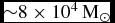 ${\sim }8 \times 10^{4} \, \mathrm{\rm M_\odot }$
is shown in orange. Its position has been shifted vertically to avoid information overload. Reproduced from Pacucci et al. (Reference Pacucci2016).
${\sim }8 \times 10^{4} \, \mathrm{\rm M_\odot }$
is shown in orange. Its position has been shifted vertically to avoid information overload. Reproduced from Pacucci et al. (Reference Pacucci2016).

3 DUST EMISSION IN z ~ 6 QUASARS
Spectra of z ~ 6 quasars reveal strong metal emission lines from the surrounding gas, with super-solar metallicityFootnote
3
and almost no evolution with redshift (e.g. Fan et al. Reference Fan2004; Juarez et al. Reference Juarez2009). This suggests vigorous recent star formation in their host galaxies which enriched quasar environment. Luminous high-redshift quasars are likely located in the densest environments in the early Universe. However, direct imaging of the stellar light of host galaxies is extremely difficult for luminous high-redshift quasars. For example, Mechtley et al. (Reference Mechtley2012) carried out deep HST/WFC3 near-infrared observations of quasar SDSS J1148+5251 (z = 6.42, hereafter J1148), attempting to detect the UV stellar continuum from young stars in the quasar host galaxy. After careful PSF subtraction, it yields a non-detection, constraining a UV-based SFR to be less than 250 $\text{M}_{\odot }$
yr−1. Similarly, Decarli et al. (Reference Decarli2012) used HST/WFC3 narrow-band imaging to search for extended Lyα nebular emission powered by star formation in the host galaxies of two luminous z ~ 6 quasars; the non-detections put a similar upper limit on the unobscured SFR in those systems.
$\text{M}_{\odot }$
yr−1. Similarly, Decarli et al. (Reference Decarli2012) used HST/WFC3 narrow-band imaging to search for extended Lyα nebular emission powered by star formation in the host galaxies of two luminous z ~ 6 quasars; the non-detections put a similar upper limit on the unobscured SFR in those systems.
On the other hand, in observed FIR to mm wavelengths, the radiation is dominated by the reprocessed radiation from cool/warm dust in the host galaxy. Assuming the dust is heated by star formation, similar to the process common in star-forming galaxies at local universe and at high redshift, the FIR to mm observations would provide the best window to study host galaxy properties while minimising contamination from the quasar light.
In the pre-ALMA era, such observations have been obtained with MAMBO, Herschel, CSO, SCUBA, Spitzer, and are limited to relatively bright sources, with continuum sensitivity around 1 mJy at observed 1 mm wavelength, corresponding to ~ 150μ in the rest-frame at z ~ 6. Wang et al. (Reference Wang2007, Reference Wang2008, Reference Wang2011a) have led a systematic search of dust emission at 250 GHz (1.2 mm) over 30 quasars at z ~ 6, covering a wide luminous range, using the MAMBO bolometer on IRAM 30-m telescope (see also Priddey et al. Reference Priddey2003; Bertoldi et al. Reference Bertoldi2003a). They found that about 1/3 of high-redshift quasar host galaxies have luminosity comparable to those of hyper-luminous IR galaxies ( $L_{\text{FIR}}= L(8\hbox{--}1\,000\,\upmu \text{m}) \sim 10^{13}$
L⊙), with the fraction remaining roughly constant from low redshift to z ~ 6. The brightest objects in the sample are also detectable in shorter wavelength with Herschel, CSO, and SCUBA, allowing a grey-body model fit to their SEDs. Figure 5 shows examples of the z ~ 6 quasar SEDs; they can be well fit with warm/cool dust at T ~ 40–50 K, consistent with the star formation providing the dust heating. This corresponds to an average dust mass of order 108 M⊙, and SFR of several hundred up to a few thousand
$L_{\text{FIR}}= L(8\hbox{--}1\,000\,\upmu \text{m}) \sim 10^{13}$
L⊙), with the fraction remaining roughly constant from low redshift to z ~ 6. The brightest objects in the sample are also detectable in shorter wavelength with Herschel, CSO, and SCUBA, allowing a grey-body model fit to their SEDs. Figure 5 shows examples of the z ~ 6 quasar SEDs; they can be well fit with warm/cool dust at T ~ 40–50 K, consistent with the star formation providing the dust heating. This corresponds to an average dust mass of order 108 M⊙, and SFR of several hundred up to a few thousand $\text{M}_{\odot }$
yr−1 for the mm bright quasars. Black hole accretion is indeed likely accompanied by intense star formation at the level expected to the formation of galactic bulge in massive galaxies, and the overall SEDs of the quasar hosts are consistent with that of Ultra-Luminous Infrared Galaxies (ULIRGs) such as Arp 220, with most of the star formation taken place in obscured phase, consistent with the HST rest-frame UV constraints.
$\text{M}_{\odot }$
yr−1 for the mm bright quasars. Black hole accretion is indeed likely accompanied by intense star formation at the level expected to the formation of galactic bulge in massive galaxies, and the overall SEDs of the quasar hosts are consistent with that of Ultra-Luminous Infrared Galaxies (ULIRGs) such as Arp 220, with most of the star formation taken place in obscured phase, consistent with the HST rest-frame UV constraints.
Examples of UV to radio SEDs of the 250 GHz detected z ~ 6 quasars. The solid and dashed grey lines show local quasar templates normalised to rest frame 1 450 Å. The thick solid line is a warm dust model normalised to the submm data and extended to the radio band with the typical radio-FIR correlation of star forming galaxies (q = 2.34; the dotted grey lines take into account factors of five excesses above and below the typical q value). Adapted from Figure 3 of Wang et al. (Reference Wang2008) and reproduced by permission of the AAS.

Wang et al. (Reference Wang2011a) also surveyed a sample of faint z ~ 6 quasars using IRAM/MAMBO (see also Omont et al. Reference Omont2013), and found that although many are not detected with high significance at 1 mJy level, stacking of all undetected sources produces a strong signal, with average flux level of ~ 0.5 mJy, that still corresponds to a high SFR of a few hundred $\text{M}_{\odot }$
yr−1. Figure 6 summarises their results of the MAMBO survey, in comparison with low-redshift sample. Overall, the FIR luminosity follows a weak dependence on the quasar bolometric luminosity (dominated by optical/UV accretion energy):
$\text{M}_{\odot }$
yr−1. Figure 6 summarises their results of the MAMBO survey, in comparison with low-redshift sample. Overall, the FIR luminosity follows a weak dependence on the quasar bolometric luminosity (dominated by optical/UV accretion energy): $L_{\text{FIR}} \sim L_{\text{bol}}^{0.6}$
. The overall FIR activity level is higher at z ~ 6 compared to local quasars at similar bolometric luminosity, suggesting a higher level of star-formation activity accompanying the growth of massive early black holes.
$L_{\text{FIR}} \sim L_{\text{bol}}^{0.6}$
. The overall FIR activity level is higher at z ~ 6 compared to local quasars at similar bolometric luminosity, suggesting a higher level of star-formation activity accompanying the growth of massive early black holes.
The FIR ( $8<\lambda _{\rm RF}<1\,000\,\upmu \text{m}$
) and bolometric quasars luminosity correlations of quasar samples from local to z ~ 6. The filled triangles and diamonds are the mean FIR luminosities for the (sub)mm detections in each sample, derived by averaging flux densities at 250 or 350 GHz. The open symbols represent the mean luminosities averaged with both the millimetre detections and non-detections in each sample. The dotted line is a fit to the local optically selected PG quasars and the dashed line shows the fit to the submillimetre or millimetre detected sources in all high-z samples and the local ULIRGs. Reproduced from Figure 4 of Wang et al. (Reference Wang2011a) by permission of the AAS.
$8<\lambda _{\rm RF}<1\,000\,\upmu \text{m}$
) and bolometric quasars luminosity correlations of quasar samples from local to z ~ 6. The filled triangles and diamonds are the mean FIR luminosities for the (sub)mm detections in each sample, derived by averaging flux densities at 250 or 350 GHz. The open symbols represent the mean luminosities averaged with both the millimetre detections and non-detections in each sample. The dotted line is a fit to the local optically selected PG quasars and the dashed line shows the fit to the submillimetre or millimetre detected sources in all high-z samples and the local ULIRGs. Reproduced from Figure 4 of Wang et al. (Reference Wang2011a) by permission of the AAS.

Complete infrared SEDs of z > 5 quasars, obtained with Herschel and Spitzer (e.g. Leipski et al. Reference Leipski2010, Reference Leipski2013), have been used to disentangle the star formation vs. AGN contribution to the total FIR emission ( $8<\lambda _{\text{RF}}<1\,000\,\upmu$
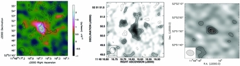
m). Leipski et al. (Reference Leipski2013) have fitted the observed SED with four distinct components: (i) a power law in the UV/optical regime to account for the accretion disk emission; (ii) a blackbody peaking in the restframe NIR to account for hot dust emission (T ~ 1300 K); (iii) a clumpy torus model to account for MIR emission arising from the AGN heated ‘dusty torus’; (iv) a modified black body to account for FIR emission powered by star formation. The result of this study is that star formation may contribute 25–60% to the bolometric FIR luminosity, with strong variations from source to source. In Figure 7, we show the results obtained in the case of J1148. The figure shows maps at 24 μm (obtained with MIPS), 100 and 160 μm (PACS), and 250 μm (SPIRE) from left to right. In this specific case, ~ 50% of the FIR emission is due to dust heated by star formation, and ~ 50% is due to the AGN heated torus.
$8<\lambda _{\text{RF}}<1\,000\,\upmu$
m). Leipski et al. (Reference Leipski2013) have fitted the observed SED with four distinct components: (i) a power law in the UV/optical regime to account for the accretion disk emission; (ii) a blackbody peaking in the restframe NIR to account for hot dust emission (T ~ 1300 K); (iii) a clumpy torus model to account for MIR emission arising from the AGN heated ‘dusty torus’; (iv) a modified black body to account for FIR emission powered by star formation. The result of this study is that star formation may contribute 25–60% to the bolometric FIR luminosity, with strong variations from source to source. In Figure 7, we show the results obtained in the case of J1148. The figure shows maps at 24 μm (obtained with MIPS), 100 and 160 μm (PACS), and 250 μm (SPIRE) from left to right. In this specific case, ~ 50% of the FIR emission is due to dust heated by star formation, and ~ 50% is due to the AGN heated torus.
Maps of J1148 at 24 μm (obtained with MIPS), 100 and 160 μm (PACS), and 250 μm (SPIRE) from left to right. All images are 2 arcmin on a side and North is to the top with East to the left. The circle indicating the position of the quasar has a diameter of 20 arcsec. PACS observations reveal the presence of a secondary object ~ 10 arcsec north-west of the quasar. A possible counterpart is also seen in the MIPS map. The source complex is also detected in the SPIRE band, but the spatial resolution is too low to identify a possible double source. Adapted from Figure 1 of Leipski et al. (Reference Leipski2013) and reproduced by permission of the AAS.

Observations of Wang et al. (Reference Wang2011a), Omont et al. (Reference Omont2013), and Leipski et al. (Reference Leipski2013) are at the limit of previous generation facilities. The majority of quasars at high redshift are still undetected individually, with potential strong selection effects from the low S/N data and non-detections, as well as possible luminosity dependent biases. ALMA has revolutionised the field of submm and mm studies of galaxies. Even in its early science observation phase, ALMA have represented a factor of > 10 increase in observing efficiency for both continuum and line detections at submm wavelengths comparing to current facilities.
Venemans et al. (Reference Venemans2016) presented sensitive ALMA observations of three quasars at 6.6 < z < 6.9 in both dust continuum and [C ii] emission. These observations reached an rms level of 0.1 mJy on the continuum. All three objects are clearly detected with SFR of 100 to 1 600 $\text{M}_{\odot }$
yr−1 based on similar assumptions to Wang et al. (Reference Wang2011a). Willott et al. (Reference Willott2015) carried out the deepest yet ALMA observations of high-redshift quasars, targeting two z ~ 6 quasars at moderate luminosity and with black hole masses an order of magnitude lower than the average in the Wang et al. (Reference Wang2011a) sample. These observations reached an rms level on 0.03 mJy on the continuum, and showed a significantly lower FIR luminosity: the 1.2 mm continuum luminosity is 0.05–0.2 mJy, corresponding to an FIR-based SFR of only 19–73
$\text{M}_{\odot }$
yr−1 based on similar assumptions to Wang et al. (Reference Wang2011a). Willott et al. (Reference Willott2015) carried out the deepest yet ALMA observations of high-redshift quasars, targeting two z ~ 6 quasars at moderate luminosity and with black hole masses an order of magnitude lower than the average in the Wang et al. (Reference Wang2011a) sample. These observations reached an rms level on 0.03 mJy on the continuum, and showed a significantly lower FIR luminosity: the 1.2 mm continuum luminosity is 0.05–0.2 mJy, corresponding to an FIR-based SFR of only 19–73 $\text{M}_{\odot }$
yr−1. Clearly, the survey at the most luminous end does not tell the whole story of the black hole-starburst connection at high redshift, and we expect that comprehensive ALMA surveys in the coming years will unveil a complete picture of star formation around SMBHs at high redshift.
$\text{M}_{\odot }$
yr−1. Clearly, the survey at the most luminous end does not tell the whole story of the black hole-starburst connection at high redshift, and we expect that comprehensive ALMA surveys in the coming years will unveil a complete picture of star formation around SMBHs at high redshift.
One assumption of all studies discussed above is that FIR dust emission in quasar hosts is powered by star formation similar to what observed in ULIRGs. As shown in Figures 5, this is consistent with the shape of quasar SED over wide wavelength range. Lyu et al. (Reference Lyu2016) fit a family of SED models that consist of AGN and starburst templates to a sample of Spitzer+Herschel+mm SEDs (Leipski et al. Reference Leipski2014) finding a dominant starburst contributions in the FIR bands probed by MAMBO and ALMA observations. On the theoretical side, Schneider et al. (Reference Schneider2015) carried out the first detailed radiative transfer model to fit the broad-band multi-wavelength SED of the well-observed quasar J1148. They found that the central AGN heating could contribute 30–70% of the observed FIR emission, but starburst contribution is still consistent with an SFR of ${\sim }1\,000\,\text{M}_{\odot }$
yr−1.
${\sim }1\,000\,\text{M}_{\odot }$
yr−1.
4 [C ii] EMISSION IN z ~ 6 QUASARS
Atomic fine structure line emission, and in particular the [C ii] 158 μm line, is thought to be the dominant coolant of the ISM, tracing the cold neutral medium and photon-dominated regions associated with star formation. The [C ii] line is the strongest ISM line in the local universe. However, because of its wavelength in the FIR, for long time it has been impossible to observe; thus, the first [C ii] detections have been limited to low-redshift galaxies from space observations (see, for example, the recent works by Herrera-Camus et al. Reference Herrera-Camus2015 and Samsonian et al. Reference Samsonian2016).
The first [C ii] observations at high redshift came from luminous quasars (e.g. Maiolino et al. Reference Maiolino2005; Walter et al. Reference Walter2006), since [C ii] becomes observable from the ground at $z>4\text{--}5$
(e.g. Iono et al. Reference Iono2006; Wagg et al. Reference Wagg2010; De Breuck et al. Reference De Breuck2011; Wagg et al. Reference Wagg2012; Cox et al. Reference Cox2011). This line is important for understanding the high-redshift universe because of its high luminosity, its connection to star formation, and the ability to acquire detailed kinematics using high spatial resolution radio interferometric observations. In particular, [C ii] observations in
$z>4\text{--}5$
(e.g. Iono et al. Reference Iono2006; Wagg et al. Reference Wagg2010; De Breuck et al. Reference De Breuck2011; Wagg et al. Reference Wagg2012; Cox et al. Reference Cox2011). This line is important for understanding the high-redshift universe because of its high luminosity, its connection to star formation, and the ability to acquire detailed kinematics using high spatial resolution radio interferometric observations. In particular, [C ii] observations in $z\sim 4\text{--}5$
quasars have shown the presence of close ( < 50 kpc) massive star-forming galaxies interacting with the quasar hosts, possibly indicating that mergers play some role in the early, fast growth of SMBHs (e.g. Gallerani et al. Reference Gallerani2012; Trakhtenbrot et al. Reference Trakhtenbrot2017b).
$z\sim 4\text{--}5$
quasars have shown the presence of close ( < 50 kpc) massive star-forming galaxies interacting with the quasar hosts, possibly indicating that mergers play some role in the early, fast growth of SMBHs (e.g. Gallerani et al. Reference Gallerani2012; Trakhtenbrot et al. Reference Trakhtenbrot2017b).
The [C ii] line is detected in quasars up to the highest redshift at z = 7.1 (Venemans et al. Reference Venemans2012; Venemans et al. Reference Venemans2017). However, before ALMA, only a handful of high-redshift quasars are detected in [C ii] (e.g. Bañados et al. Reference Bañados2015; Wang et al. Reference Wang2016) and only J1148 has sufficiently high S/N and resolution for detailed analysis of its host galaxy ISM properties (Walter et al. Reference Walter2009; Maiolino et al. Reference Maiolino2012).
Three early ALMA results highlight the power of using [C ii] as a probe of star formation in high-redshift quasar host galaxies and the co-evolution of SMBHs and galaxies at early epoch. The [C ii] luminosity of z ~ 6 quasars observed with ALMA (Wang et al. Reference Wang2013; Willott et al. Reference Willott2015; Venemans et al. Reference Venemans2016) ranges from 0.6 to 8.7 $\times 10^9\,\text{L}_{\odot }$
. In all cases, [C ii] lines are clearly resolved with FWHM ranging from 190 to 520 km s−1. In Table 1, we report all the detections of [C ii] emission obtained so far in z ~ 6 quasars along with their black hole masses.
$\times 10^9\,\text{L}_{\odot }$
. In all cases, [C ii] lines are clearly resolved with FWHM ranging from 190 to 520 km s−1. In Table 1, we report all the detections of [C ii] emission obtained so far in z ~ 6 quasars along with their black hole masses.
Black hole masses (M
BH), [C ii ] luminosities ( $L_{\rm [C\,{\sc II}]}$
), [C ii ] line widths (FWHM
$L_{\rm [C\,{\sc II}]}$
), [C ii ] line widths (FWHM $_{\rm [C\,{{\sc II}}}$
) of z ~ 6 quasars.
$_{\rm [C\,{{\sc II}}}$
) of z ~ 6 quasars.

a First and second labels represent references for M BH and [C ii] observations, respectively.
b See Venemens et al. (2017) for follow-up observations. References: [1] De Rosa et al. (2014); [2] Venemans et al. (Reference Venemans2012); [3] Venemans et al. (Reference Venemans2016); [4] Venemans et al. (Reference Venemans2015b); [5] Bañados et al. (Reference Bañados2015); [6] Willott et al. (2010); [7] Willott et al. (Reference Willott2013); [8] Wu et al. (Reference Wu2015); [9] Wang et al. (Reference Wang2016); [10] Willott et al. (Reference Willott2015); [11] Wang et al. (Reference Wang2013).
By combining the [C ii] and FIR luminosity measurements, it has been possible to compare the $L_{\text{C\,\textsc {ii}}}/L_{\text{FIR}}$
ratio of z ≳ 6 quasars with results obtained in local galaxies (see Figure 8). It results that the
$L_{\text{C\,\textsc {ii}}}/L_{\text{FIR}}$
ratio of z ≳ 6 quasars with results obtained in local galaxies (see Figure 8). It results that the $L_{\text{C\,\textsc {ii}}}/L_{\text{FIR}}$
ratio follows the low-redshift trend of decreasing towards FIR brighter objects. The origins of this effect, generally called ‘[C ii] deficit’, are not definitively understood and it is still not clear whether it is driven by the presence of an X-ray source or simply by specific galaxy ISM properties. For instance, the central AGN may provide a substantial contribution to the dust heating and FIR emission, determining a lower
$L_{\text{C\,\textsc {ii}}}/L_{\text{FIR}}$
ratio follows the low-redshift trend of decreasing towards FIR brighter objects. The origins of this effect, generally called ‘[C ii] deficit’, are not definitively understood and it is still not clear whether it is driven by the presence of an X-ray source or simply by specific galaxy ISM properties. For instance, the central AGN may provide a substantial contribution to the dust heating and FIR emission, determining a lower $L_{\text{C\,\textsc {ii}}}/L_{\text{FIR}}$
ratio in the nuclear region (e.g. Sargsyan et al. Reference Sargsyan2012) and/or its strong X-ray radiation may reduce the C ii abundance (e.g. Langer & Pineda Reference Langer and Pineda2015). Moreover, compact starbursts tend to show substantially smaller
$L_{\text{C\,\textsc {ii}}}/L_{\text{FIR}}$
ratio in the nuclear region (e.g. Sargsyan et al. Reference Sargsyan2012) and/or its strong X-ray radiation may reduce the C ii abundance (e.g. Langer & Pineda Reference Langer and Pineda2015). Moreover, compact starbursts tend to show substantially smaller $L_{\text{C\,\textsc {ii}}}/L_{\text{FIR}}$
ratios with respect to extended and more diffuse systems (e.g. Díaz-Santos et al. Reference Díaz-Santos2013). Finally, also the ISM metallicity can affect both [C ii] and FIR emissions, though its final role on the ‘[C ii] deficit’ is controversial (e.g. De Breuck et al. Reference De Breuck2011; Vallini et al. Reference Vallini2015). Given the large scatter of the observed
$L_{\text{C\,\textsc {ii}}}/L_{\text{FIR}}$
ratios with respect to extended and more diffuse systems (e.g. Díaz-Santos et al. Reference Díaz-Santos2013). Finally, also the ISM metallicity can affect both [C ii] and FIR emissions, though its final role on the ‘[C ii] deficit’ is controversial (e.g. De Breuck et al. Reference De Breuck2011; Vallini et al. Reference Vallini2015). Given the large scatter of the observed $L_{\text{C\,\textsc {ii}}}/L_{\text{FIR}}$
ratio at any given FIR luminosity, further observations are required to reach any conclusive understanding of the ‘[C ii] deficit’ origins (see further discussions in Trakhtenbrot et al. Reference Trakhtenbrot2017b, Narayanan & Krumholz Reference Narayanan and Krumholz2017, Brisbin et al. Reference Brisbin2015, Graciá-Carpio et al. Reference Graciá-Carpio2011, and Luhman et al. Reference Luhman2003).
$L_{\text{C\,\textsc {ii}}}/L_{\text{FIR}}$
ratio at any given FIR luminosity, further observations are required to reach any conclusive understanding of the ‘[C ii] deficit’ origins (see further discussions in Trakhtenbrot et al. Reference Trakhtenbrot2017b, Narayanan & Krumholz Reference Narayanan and Krumholz2017, Brisbin et al. Reference Brisbin2015, Graciá-Carpio et al. Reference Graciá-Carpio2011, and Luhman et al. Reference Luhman2003).
The relation between FIR luminosity and the ratio of [C ii] to FIR luminosity at different redshift. The horizontal dashed line show the average value of the [C ii] to FIR ratio found in local star-forming galaxies. Reproduced from Figure 5 of Venemans et al. (Reference Venemans2016) by permission of the authors and the AAS.

In the left panels of Figure 9, we show the [C ii] line spectra of the Wang et al. (Reference Wang2013) sample, compared with their CO (6–5) observations from PdBI. In the middle panels, [C ii] emission maps of the same sources are presented. The right panels show the velocity maps of the Wang et al. (Reference Wang2013) sample. In fact, an especially exciting aspect of ALMA [C ii] observations is the ability of spatially resolve the host galaxy kinematics. In the bright sample of Wang et al. (Reference Wang2013), four of the five sources are spatially resolved under subarcsec resolution, with a deconvolved size of 2–4 kpc. For those that are resolved in [C ii], a clear velocity gradient is evident across the image, consistent with a strong velocity shear due to either rotation or strong galaxy interaction.
Left panels: [C ii] line spectra (black solid line) of the five ALMA detected quasars, together with the previous CO (6–5) detections from PdBI (blue dotted line, scaled to the [C ii] line) and a Gaussian fit to the [C ii] line (red dashed line). Middle panels: [C ii] line velocity-integrated map. Right panels: Line intensity-weighted velocity maps using pixels detected at ⩾ 4σ. Adapted from Figures 2 and 5 of Wang et al. (Reference Wang2013) and reproduced by permission of the AAS.

We note that two of the z > 6.6 quasars in the Venemans et al. (Reference Venemans2016) sample are also resolved with similar size measurements. However, their velocity structures are not consistent with a flat rotation curve. In addition, one object shows a large (1 700 km s −1) velocity shift between [C ii] redshift and the redshift of the Mgii low-ionisation line, usually used as standard quasar systematic redshift. This wide range of morphology points to a large diversity of quasar host galaxy properties, potentially linked to the different evolutionary stages of host galaxy assembly. For two fainter objects in Willott et al. (Reference Willott2015), one is resolved (with similar size) and the other marginally resolved due to low S/N.
With constraints on both sizes and velocity line width, one can make crude estimates of the dynamical mass of the host galaxy (1.3 × 10¹⁰ < M
dyn/M⊙ < 1.2 × 10¹¹), and place these high redshift quasars onto the equivalent of $M_{\text{BH}}$
− σ or
$M_{\text{BH}}$
− σ or $M_{\text{BH}}$
−
$M_{\text{BH}}$
− $M_{\text{dyn}}$
relations established at low redshift. Figure 10 shows the
$M_{\text{dyn}}$
relations established at low redshift. Figure 10 shows the $M_{\text{BH}}$
−
$M_{\text{BH}}$
− $M_{\text{dyn}}$
relation at z ~ 6: luminous high-redshift quasars systematically deviate from the local relation in the sense that their host mass is low compared to local galaxies of the same black hole mass. This seems to imply that at least for the luminous systems observed here, black hole growth precedes galaxy assembly and quasars with the largest black holes are not necessarily in the most massive galaxies in early epochs. However, there are a number of caveats in reaching any firm conclusion with regard to the evolution of black hole/galaxy mass relation, given the still limited quality of spatially resolved data, the potential complex gas kinematics and the luminosity bias when targeting a flux selected sample. In particular, estimates of the stellar mass in z ≳ 5 quasars by Lyu et al. (Reference Lyu2016), based on the infrared SED fitting, provide BH-galaxy mass ratios consistent with the local relation. Moreover, Valiante et al. (Reference Valiante2014) suggested that since observations of high- z QSOs are sensitive to the innermost 2.5–3 kpc, they are simply missing the galaxy star formation located on larger scales. Interestingly, the fainter quasars with lower black hole masses observed in Willott et al. (Reference Willott2015) have similar [C ii] line width and size constraints.
$M_{\text{dyn}}$
relation at z ~ 6: luminous high-redshift quasars systematically deviate from the local relation in the sense that their host mass is low compared to local galaxies of the same black hole mass. This seems to imply that at least for the luminous systems observed here, black hole growth precedes galaxy assembly and quasars with the largest black holes are not necessarily in the most massive galaxies in early epochs. However, there are a number of caveats in reaching any firm conclusion with regard to the evolution of black hole/galaxy mass relation, given the still limited quality of spatially resolved data, the potential complex gas kinematics and the luminosity bias when targeting a flux selected sample. In particular, estimates of the stellar mass in z ≳ 5 quasars by Lyu et al. (Reference Lyu2016), based on the infrared SED fitting, provide BH-galaxy mass ratios consistent with the local relation. Moreover, Valiante et al. (Reference Valiante2014) suggested that since observations of high- z QSOs are sensitive to the innermost 2.5–3 kpc, they are simply missing the galaxy star formation located on larger scales. Interestingly, the fainter quasars with lower black hole masses observed in Willott et al. (Reference Willott2015) have similar [C ii] line width and size constraints.
The black hole mass vs. dynamical mass relation of z ~ 6 quasars. The black diamonds are values obtained for local galaxies (taken from Kormendy & Ho Reference Kormendy and Ho2013). The solid line and the shaded area shows the local $M_{\text{BH}}$
vs.
$M_{\text{BH}}$
vs. $M_{\text{bulge}}$
relation derived by Kormendy & Ho (Reference Kormendy and Ho2013). Reproduced from Figure 12 of Venemans et al. (Reference Venemans2016) by permission of the authors and the AAS.
$M_{\text{bulge}}$
relation derived by Kormendy & Ho (Reference Kormendy and Ho2013). Reproduced from Figure 12 of Venemans et al. (Reference Venemans2016) by permission of the authors and the AAS.

5 EVIDENCE FOR QUASAR FEEDBACK AT z ~ 6
Quasars are invoked by most models and numerical simulations to quench star formation in massive galaxies, through massive radiation-pressure driven outflows. The resulting system, cleaned of cold gas, is expected to passively evolve into local massive elliptical galaxies (e.g. Silk & Rees Reference Silk and Rees1998; Granato et al. Reference Granato2004; Di Matteo et al. Reference Di Matteo2005; King et al. Reference King2011; Zubovas & King Reference Zubovas and King2012; Fabian Reference Fabian2015). This process is also thought to contribute to the steeply declining mass function of galaxies at high masses, by preventing the overgrowth of galaxies. By halting both star formation and black hole accretion, this process may also be responsible for the correlation between black hole and stellar mass in the host spheroid.
Evidence for quasar-driven outflows has been found in local systems, especially through the discovery of massive and powerful winds traced by the cold phase of the ISM (Sturm et al. Reference Sturm2011; Feruglio et al. Reference Feruglio2010; Cicone et al. Reference Cicone2014). These examples are only local ‘laboratories’ of quasar-driven outflows. However, in order to explain the properties of local elliptical massive galaxies (which have an old stellar population), the bulk of the star-formation quenching must occur at high redshift (z ~ 2). Evidence for massive outflows at high redshift is much more sparse. Although quasar-driven outflows have been seen in z ~ 2 quasars, these are generally traced by the ionised phase (generally through the [Oiii] 5007 Å or Ly α lines, Cano-Diaz et al. Reference Cano-Diaz2012; Harrison et al. Reference Harrison2014; Brusa et al. Reference Brusa2015; Carniani et al. Reference Carniani2015; Carniani et al. Reference Carniani2016; Swinbank et al. Reference Swinbank2015), which generally probes only a small fraction of the outflowing mass. Evidence of molecular outflows has been found in a few targets at z ~ 2.3 (Weiss et al. Reference Weiss2012, George et al. 2012). However, the discovery of passive and old (age 2–3 Gyr) galaxies at z ~ 2.5, when the age of the Universe was only ~ 3 Gyr (Kriek et al. Reference Kriek2006; Labbe et al. Reference Labbe2005; Saracco et al. Reference Saracco2005; Cimatti et al. Reference Cimatti2004), implies that quenching by quasar-driven outflows must have already been in place at z ~ 6, at least in a fraction of very massive galaxies. Evidence for quasar-driven massive outflows has been recently found at z > 6, in J1148 (Maiolino et al. Reference Maiolino2012; Cicone et al. Reference Cicone2015). This outflow has been identified through the detection of broad wings of the [C ii] line (Figure 11), tracing cold gas expelled at velocities higher than 1 000 km s −1 (see Table 2). The map of the [C ii] emission extends over a region of about 30 kpc (left panel of Figure 12). However, most of this extended emission is associated with the high velocity gas, as shown in the right panel of Figure 12, implying that the outflow in this system is well developed and that cold gas has been driven out to very large distances from the central active region. The inferred outflow rate is very large (1400±300M⊙yr−1), comparable to or exceeding the SFR. The implied depletion time of the gas in the host galaxy would be shorter than 10 million yrs (assuming that there is no additional gas supply and that the outflow rate continues at this rate, but see additional discussion below on this regard), implying that star formation would be quenched on very short timescales. Interestingly, these observations are consistent with the expectations of models and simulations of the formation of massive galaxies in the early Universe accompanied by black hole growth. More specifically, models expect a similar very high quasar-driven outflow rate (Figure 13, Valiante et al. Reference Valiante2012, while expecting a negligible contribution from SN-driven winds) and similar outflow velocities and outflow extension (Figure 14, Costa et al. Reference Costa2015).
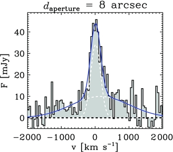
IRAM PdBI continuum-subtracted spectrum of the [C ii] 158 μm emission line of J1148. The spectrum shown has been extracted using a circular aperture with a diameter of 8 arcsec. For display purposes, the spectrum has been re-binned into channels of 46.8 km s −1. The Gaussian fits to the line profiles (using a narrow and a broad Gaussian component to fit respectively the narrow core, tracing quiescent gas, and the broad wings, tracing the outflow) are performed on the original non-binned spectrum (channels of 23.4 km s −1). Adapted from Figure 1 of Cicone et al. (Reference Cicone2015). Credit: Cicone Claudia, A&A, 574, 14, 2015, reproduced with permission © ESO.
Left: IRAM PdBI continuum-subtracted map of the total [C ii] 158 μm emission of J1148, integrated within v ∈ ( − 1400, 1200) km s −1. Negative and positive contours are in steps of 3 σ (1 σ rms noise is 0.26 Jy beam −1 km s −1). The synthesised beam ( 1.3arcmin × 1.2 arcmin) is shown in the bottom left corner of the map. The cross indicates the pointing and phase centre, corresponding to the optical position of the quasar. Adapted from Figure 2 of Cicone et al. (Reference Cicone2015). Right: [C ii] map obtained by integrating only the high velocity wings, within [ − 1 400, − 300] km s −1 and within [400,1 200] km s −1, revealing the outflow extension. Adapted from Figure 5 of Cicone et al. (Reference Cicone2015). Credit: Cicone Claudia, A&A, 574, 14, 2015, reproduced with permission © ESO.

Model developed by Valiante et al. (Reference Valiante2012) showing the evolution of the quasar-driven (red) and SN-driven (blue) outflow rates for a system with properties similar to J1148. The outflow rate observed in J1148 is indicated with a blue symbol as a lower limit, since the additional contribution to the outflow rate from other gas phases is not known. Adapted from Figure 3 of Valiante et al. (Reference Valiante2012) and reproduced by permission of the authors.

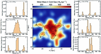
Simulation of the cold gas distribution in a quasar host galaxy at z = 6.4 (map in the middle). Figures on the left and right columns show the gas velocity distribution in some regions of the field of view, revealing that the outflowing gas can indeed reach velocities of about 1000 km s −1. Reproduced from Figure 3 of Costa et al. (Reference Costa2015).
Another interesting result, also going in the direction of reducing the efficiency of quasar feedback, is that the outflow activity appears to be episodic/bursty and not continuous. This could be observationally inferred by measuring the dynamical time (distance from the centre divided by outflowing velocity) of the individual outflowing clouds in J1148 (Cicone et al. Reference Cicone2015). This analysis enables the outflow activity to be traced ‘back in time’. The results are shown in Figure 15 for the evolution of the mass outflow rate, kinetic power, and momentum rate. Although various selection and sensitivity issues potentially affect the uncertainties associated with these quantities, the diagrams in Figure 15 suggest that the outflow has been active only for the last 30 Myr, and in a bursty mode.
Mass outflow rate (left), kinetic power (normalised to the AGN radiative luminosity, middle) and momentum rate (normalised to $L_{\text{AGN}}/c$
, right) as a function of the dynamical time of the [C ii] outflowing clumps, as observed in J1148. Reproduced from Figure 7 of Cicone et al. (Reference Cicone2015). Credit: Cicone Claudia, A&A, 574, 14, 2015, reproduced with permission © ESO.
$L_{\text{AGN}}/c$
, right) as a function of the dynamical time of the [C ii] outflowing clumps, as observed in J1148. Reproduced from Figure 7 of Cicone et al. (Reference Cicone2015). Credit: Cicone Claudia, A&A, 574, 14, 2015, reproduced with permission © ESO.

6 MOLECULAR GAS IN z ~ 6 QUASAR HOSTS
The carbon monoxide (CO) is the most abundant molecule after molecular hydrogen ( $\text{H}_2$
) and its rotational transitions are excited through collisions with
$\text{H}_2$
) and its rotational transitions are excited through collisions with $\text{H}_2$
. Thus, rest frame FIR lines arising from rotational transitions in the CO molecule can be used to measure the
$\text{H}_2$
. Thus, rest frame FIR lines arising from rotational transitions in the CO molecule can be used to measure the $\text{H}_2$
abundance (in the case of low- J transitions) and to constrain the excitation conditions of molecular gas (in the case of high- J transitions).
$\text{H}_2$
abundance (in the case of low- J transitions) and to constrain the excitation conditions of molecular gas (in the case of high- J transitions).
6.1 Low- J (J ⩽ 7) CO lines
CO lines have been observed in several z ~ 6 quasars at different total angular momentum J. The first CO detections in a z ~ 6 quasar has been obtained by Bertoldi et al. (Reference Bertoldi2003b) and Walter et al. (Reference Walter2003) in J1148. These authors detected the CO(6–5) and CO(7–6) with the PdBI and the CO(3–2) with the VLA, respectively (see right-most and middle panels of Figure 16). In the same object, an upper flux limit for the CO (1–0) line was obtained from observations with the Effelsberg 100-m telescope. More recently, Stefan et al. (Reference Stefan2015) have detected the CO(2–1) transition (see the left-most panel of Figure 16). The angular resolution of the CO(2–1) and CO(3–2) lines is high enough to resolve the CO emission and provide estimates on the spatial extent of the $\text{H}_2$
distribution in this high- z quasar that results to be ⩽ 4kpc. Moreover, the intensity of the lines is consistent with
$\text{H}_2$
distribution in this high- z quasar that results to be ⩽ 4kpc. Moreover, the intensity of the lines is consistent with $\text{H}_2$
masses ~ 2 × 10¹⁰M⊙. This large amount of molecular gas is common to high- z quasars, since similar results have been obtained in ~ 20 quasars at 5.7 < z < 6.2 (Wang et al. Reference Wang2010, Reference Wang2011a, Reference Wang2011b, Reference Wang2013, see Figure 17).
$\text{H}_2$
masses ~ 2 × 10¹⁰M⊙. This large amount of molecular gas is common to high- z quasars, since similar results have been obtained in ~ 20 quasars at 5.7 < z < 6.2 (Wang et al. Reference Wang2010, Reference Wang2011a, Reference Wang2011b, Reference Wang2013, see Figure 17).
Detections of CO emission in J1148 at z = 6.4. Left panel: VLA observations of the CO(2-1) transition. Reproduced from Figure of 4 from Stefan et al. (Reference Stefan2015). Middle panel: CO(3-2) emission obtained with the same instrument. Reproduced from Figure 1 of Walter et al. (Reference Walter2004) and reproduced by permission of the AAS. Right panel: CO(6-5) emission detected with PdBI. Reproduced from Figure 2 of Bertoldi et al. (Reference Bertoldi2003b). Credit: Bertoldi Frank, A&A, 409, 47, 2003, reproduced with permission © ESO.
PdBI observation of the CO (6–5) line from J2310+1855. The left panel shows the CO (6–5) line spectrum binned to 30 kms−1 channels. The solid line is a Gaussian fit to the line spectrum. The right panel shows the intensity map of the CO (6–5) line emission. The 1 σ rms noise of the map is 0.13Jykms−1Beam−1 and the contours in steps of 2 σ. The beam size of $\rm 5.4\,\text{arcsec}\times 3.9$
arcsec is plotted on the bottom left. The cross denotes the position of the optical quasar. Reproduced from Figure 1 of Wang et al. (Reference Wang2013) and reproduced by permission of the AAS.
$\rm 5.4\,\text{arcsec}\times 3.9$
arcsec is plotted on the bottom left. The cross denotes the position of the optical quasar. Reproduced from Figure 1 of Wang et al. (Reference Wang2013) and reproduced by permission of the AAS.

6.2 High- J (J > 7) CO lines
High- J CO lines arise from states > 100 K above ground and have critical densities > 105cm−3. These lines trace the warm, denser molecular gas in the centre of galaxies, and are difficult to excite solely with star formation. Thus, they can be used to test models that distinguish between AGN and starburst systems (e.g. Meijerink et al. Reference Meijerink2009; Schleicher et al. Reference Schleicher2010a). More specifically, a quantity that is generally used to investigate the excitation conditions of the molecular gas is the so-called CO Spectral Line Energy Distribution (COSLED). This quantity is defined as the ratio of the (J → J − 1) CO rotational transition luminosity to a fixed CO transition. The COSLED represents a powerful tool to investigate the molecular gas kinetic temperature, $T_\text{K}$
, that depends on the radiative heating due to stars and AGN (e.g. Obreschkow et al. Reference Obreschkow2009). More specifically, a higher
$T_\text{K}$
, that depends on the radiative heating due to stars and AGN (e.g. Obreschkow et al. Reference Obreschkow2009). More specifically, a higher $T_\text{K}$
boosts higher J transitions, thus pushing the COSLED maximum towards larger J values. The presence of high energy ( ⩾ 1keV) photons emitted by an AGN causes the CO line intensities to rise well beyond J = 10, making these highly excited lines powerful probes of quasar activity and sensitive tracers of X-ray Dominated Regions (XDR) (e.g. Schleicher et al. Reference Schleicher2010a).
$T_\text{K}$
boosts higher J transitions, thus pushing the COSLED maximum towards larger J values. The presence of high energy ( ⩾ 1keV) photons emitted by an AGN causes the CO line intensities to rise well beyond J = 10, making these highly excited lines powerful probes of quasar activity and sensitive tracers of X-ray Dominated Regions (XDR) (e.g. Schleicher et al. Reference Schleicher2010a).
High- J CO lines are commonly detected in the local Universe up to J = 30 (e.g. Panuzzo et al. Reference Panuzzo2010; Meijerink et al. Reference Meijerink2013; Hailey-Dunsheath et al. Reference Hailey-Dunsheath2012; Mashian et al. Reference Mashian2015). At higher redshifts, the highest- J CO lines observed are the CO(17–16) in J1148 at z = 6.4 (Gallerani et al. Reference Gallerani2014) and the CO(11–10) in APM 08279+5255 at z = 3.9 (Weiss et al. Reference Weiss2007).
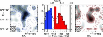
While observing the dust continuum emission in J1148 with the PdBI receivers tuned at ~ 262 GHz, Gallerani et al. (Reference Gallerani2014) serendipitously detected strong line emission in the data, with a significance of 6.2 σ (see Figure 18). This strong unexpected emission has been ascribed to the sum of the CO(17–16) emission line (νRF = 1956.018137 GHz), and five OH+ rotational transitions (1953.426326 ⩽ νRF/GHz ⩽ 1959.675435) for a total velocity-integrated flux of the system of S Δv = 1.01±0.16 Jy km s −1 (see Gallerani et al. Reference Gallerani2014 for further details).
Left panel: PdBI CO(17–16) emission detected in J1148. The 1 σ noise in the images is 0.183 mJy beam −1 and contours are plotted from − 1σ to 6 σ. The cross indicates the optical position of J1148. The beam ( $1.1\,\text{arcsec}\!\times \!0.98$
arcsec) is plotted in the lower left of the panel). Right panel: Spectrum of the CO(17–16) line of J1148 as observed with the PdBI (channel width: 39 MHz = 44 km s −1, noise per channel: 0.8 mJy), shown on the top of a 4.0 ±0.1 mJy continuum emission at 262 GHz. Adapted from Gallerani et al. (Reference Gallerani2014).
$1.1\,\text{arcsec}\!\times \!0.98$
arcsec) is plotted in the lower left of the panel). Right panel: Spectrum of the CO(17–16) line of J1148 as observed with the PdBI (channel width: 39 MHz = 44 km s −1, noise per channel: 0.8 mJy), shown on the top of a 4.0 ±0.1 mJy continuum emission at 262 GHz. Adapted from Gallerani et al. (Reference Gallerani2014).

In the middle panel of Figure 19, the observed spectrum rebinned to 88 km s −1 is shown. The data have been fitted through a double Gaussian. The dotted line (shaded red region) represents the CO(17–16) line ( $z_{\rm CO(17\text{--}16)}\sim 6.418$
; FWHM
$z_{\rm CO(17\text{--}16)}\sim 6.418$
; FWHM $_{\rm CO(17\text{--}16)}\sim 297$
km s −1), while the dashed line (blue shaded region) denotes the OH + line (z
OH+
~ 6.420; FWHM OH+
~ 373 km s −1). The relative contribution of the CO(17–16) line to the total emission results to be ~ 40%, that corresponds to a CO(17–16) luminosity
$_{\rm CO(17\text{--}16)}\sim 297$
km s −1), while the dashed line (blue shaded region) denotes the OH + line (z
OH+
~ 6.420; FWHM OH+
~ 373 km s −1). The relative contribution of the CO(17–16) line to the total emission results to be ~ 40%, that corresponds to a CO(17–16) luminosity $L_{\rm CO(17\text{--}16)}=(4.9\;\pm\; 1.1)\times 10^8\,\text{L}_{\odot }$
(Solomon et al. Reference Solomon1992).
$L_{\rm CO(17\text{--}16)}=(4.9\;\pm\; 1.1)\times 10^8\,\text{L}_{\odot }$
(Solomon et al. Reference Solomon1992).
Middle panel: Spectrum shown in Figure 18, zoomed in the rest frame frequency range $1\,953<\nu _{\text{RF}}/[\text{GHz}]<1\,961$
, assuming z = 6.4189 for the J1148 redshift. Vertical lines show the frequencies of five OH + transitions and the CO(17–16) transition (νRF = 1956.018137 GHz). Left panel: OH + map obtained by integrating over the channels denoted by the blue shaded region in the middle panel. Right panel: CO(17–16) map obtained by integrating over the channels denoted by the red shaded region in the middle panel.
$1\,953<\nu _{\text{RF}}/[\text{GHz}]<1\,961$
, assuming z = 6.4189 for the J1148 redshift. Vertical lines show the frequencies of five OH + transitions and the CO(17–16) transition (νRF = 1956.018137 GHz). Left panel: OH + map obtained by integrating over the channels denoted by the blue shaded region in the middle panel. Right panel: CO(17–16) map obtained by integrating over the channels denoted by the red shaded region in the middle panel.
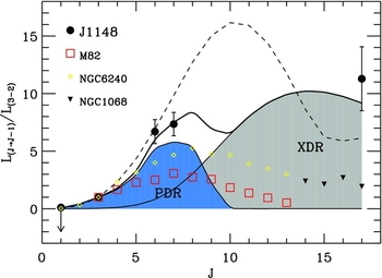
By combining all the CO observations obtained in J1148 (see Table 2), it has been possible to construct its COSLED, shown in Figure 20 with filled circles, normalised to the CO(3–2) transition. These data have been interpreted by comparing them with results of radiative transfer calculations of Photo-Dissociation Regions (PDR, i.e. excited by UV radiation field) and XDR(i.e. excited by X-ray photons) developed by Meijerink et al. (Reference Meijerink2005, Reference Meijerink2007). For this comparison, different gas densities (n PDR, n XDR in cm−3), UV fluxes (G 0 in Habing units of 1.6 × 10⁻³ergs−1cm−2), and X-ray fluxes (F X in ergs−1cm−2) at the cloud surface have been considered.
CO Spectral Line Energy Distribution (COSLED) of J1148. Circles denote observations of several CO transitions: CO(1–0) (upper limit from Bertoldi et al. Reference Bertoldi2003b); CO(3–2) (Walter et al. Reference Walter2003); CO(6–5) (Bertoldi Reference Bertoldi2003b); CO(7–6); CO(17–16) (Gallerani et al. Reference Gallerani2014). The dashed line shows the best-fit obtained in the PDR model case, while the thick solid line represents the best-fitting composite model: the relative contributions from PDR and XDR are shown by the blue and gray shaded regions, respectively. The detection of the CO(17–16) line can not be reproduced by the PDR model alone, thus suggesting contribution from XDRs. Empty squares, empty diamonds, filled triangles show the COSLED observed in several local galaxies. Adapted from Gallerani et al. (Reference Gallerani2014).
[C ii ] and CO line fluxes and width in SDSS J1148+5251.
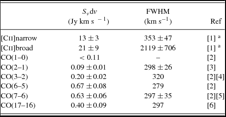
References: [1] Cicone et al. (Reference Cicone2015); [2] Bertoldi et al. (Reference Bertoldi2003b)b; [3] Stefan et al. (2016)c; [4] Walter et al. (Reference Walter2003)b; [5] Riechers et al. (Reference Riechers2009); [6] Gallerani et al. (Reference Gallerani2014).
a We report the velocity-integrated flux for the narrow and broad component obtained when the [C ii] spectrum is extracted with a circular aperture having a diameter 8 arcsec large (see Section 5 and Table 1 in Cicone et al. Reference Cicone2015).
b From Table 1 in Riechers et al. (Reference Riechers2009).
c Stefan et al. (2016) reported a velocity-integrated flux of 94.6 ±7.7 mJy beam −1 km s −1, for a beam size 1.07 and 0.97 arcsec.
The result of this comparison is that PDR models alone (dashed line in Figure 20) can not fairly explain the observed high-J (J ⩾ 7) CO line observations. Vice versa, the COSLED predicted by a model in which the molecular cloud (MC) emission is the sum of the contribution from a higher density XDR region embedded in a more rarefied and extended PDR envelope (solid line in Figure 20) is in very good agreement with observed data. According to this model, individual MCs have a typical mass M c ~ 2 × 10⁵M⊙ and a radius r c ~ 10 pc; the XDR core (n XDR = 104.25±0.25) is irradiated by an X-ray flux F X = 160±70, while the FUV flux at the PDR surface (n PDR = 103.25±0.25) is G 0 = 104.0±0.25.
The most straightforward interpretation of this result is that the detection of a prominent J ⩾ 7 line in high-redshift objects strongly supports the presence of AGN activity. According to this extremely appealing possibility, high-J CO lines could allow to identify the progenitors ( $M_{\bullet }\sim 10^{6-7} \text{M}_{\odot }$
) of SMBHs observed in z ~ 6 quasars. In Figure 21, the expected X-ray flux of the elusive SMBH progenitors is compared with their expected CO(17–16) line luminosity. Given that the luminosity of the CO(17–16) line in these objects can be as high as
$M_{\bullet }\sim 10^{6-7} \text{M}_{\odot }$
) of SMBHs observed in z ~ 6 quasars. In Figure 21, the expected X-ray flux of the elusive SMBH progenitors is compared with their expected CO(17–16) line luminosity. Given that the luminosity of the CO(17–16) line in these objects can be as high as $10^{7.5}\le L_{\rm CO(17 16)}/\text{L}_{\odot } \le 10^{8.5}$
, they should be detectable with the ALMA full array in an observing time of 12 h ⩾ t ⩾ 10 min.
$10^{7.5}\le L_{\rm CO(17 16)}/\text{L}_{\odot } \le 10^{8.5}$
, they should be detectable with the ALMA full array in an observing time of 12 h ⩾ t ⩾ 10 min.
Observed soft X-ray flux (F
soft
X) vs. CO(17–16) luminosity ( $L_{\rm CO(17\text{--}16)}$
) computed in the case of a z = 7 quasar, powered by a 3 × 10⁶M⊙ black hole, and considering an obscuring gas column density N
H > N*H = 1024 cm −2. Symbols and colours show different interstellar medium properties of the host galaxy: yellow, orange, violet, and magenta symbols refer to increasing XDR densities in the range 105.25 < n
XDR/cm−3 < 106; triangles, downwards triangles, rightwards triangles, diamonds, squares, circles represent increasing X-ray fluxes at the illuminated surface of the XDR in the range 5 < FX
< 160ergs−1cm−2. Error bars have been computed by considering the contribution of different PDR densities (103 < n
PDR/cm−3 < 103.5) to the
$L_{\rm CO(17\text{--}16)}$
) computed in the case of a z = 7 quasar, powered by a 3 × 10⁶M⊙ black hole, and considering an obscuring gas column density N
H > N*H = 1024 cm −2. Symbols and colours show different interstellar medium properties of the host galaxy: yellow, orange, violet, and magenta symbols refer to increasing XDR densities in the range 105.25 < n
XDR/cm−3 < 106; triangles, downwards triangles, rightwards triangles, diamonds, squares, circles represent increasing X-ray fluxes at the illuminated surface of the XDR in the range 5 < FX
< 160ergs−1cm−2. Error bars have been computed by considering the contribution of different PDR densities (103 < n
PDR/cm−3 < 103.5) to the $L_{\rm CO(17\text{--}16)}$
luminosity. Adapted from Gallerani et al. (Reference Gallerani2014).
$L_{\rm CO(17\text{--}16)}$
luminosity. Adapted from Gallerani et al. (Reference Gallerani2014).

7 SUMMARY AND FUTURE PROSPECTS
In this paper, we have reviewed the physical properties of the highest redshift ( $z\sim 6\text{--}7$
) quasars known so far. First of all, we have discussed the formation and evolution scenarios of the black holes that power high- z quasars, with special emphasis on the formation of massive (
$z\sim 6\text{--}7$
) quasars known so far. First of all, we have discussed the formation and evolution scenarios of the black holes that power high- z quasars, with special emphasis on the formation of massive ( ${\sim }10^3\text{--}10^5 \, \mathrm{M_{\odot }}$
) black hole seeds through the DCBH mechanism. Then, we have focussed on several properties of high- z quasars as inferred by submm and mm observations. Here below, we summarise the main results.
${\sim }10^3\text{--}10^5 \, \mathrm{M_{\odot }}$
) black hole seeds through the DCBH mechanism. Then, we have focussed on several properties of high- z quasars as inferred by submm and mm observations. Here below, we summarise the main results.
-
(i) Formation and evolution of SMBH seeds.
The DCBH channel is nowadays object of great interest in the community, above all because DCBH observational properties may be tested with current or upcoming instruments. In this context, we have discussed the case of CR7, a z = 6.6 Lyman-alpha emitter that has been indicated as a very good DCBH candidate by several studies in the last year. In particular, its Ly α and He ii luminosity are compatible with a BH born from a DCBH seed (Pallottini et al. Reference Pallottini2015). In the future, deeper X-ray observations and/or variability studies of this source may reveal its real nature. Moreover, very recently, a photometric method to select DCBH candidates in deep multi-wavelength fields has been proposed. This method has already identified a couple of DCBH candidates, at redshift z > 6; its extension to additional multi-wavelength fields will surely lead to the identification of more DCBH candidates. Nonetheless, only a spectroscopic study of the pre-selected sources will be able to confirm their real nature.
-
(ii) Dust continuum emission.
Dust continuum emission studies have revealed that high- z quasars have FIR luminosities L FIR ~ 1012 − 1013L⊙ that correspond to dust masses ~ 108M⊙ and SFR of few hundred up to few thousands M⊙yr−1. These studies have also shown that the FIR activity of high- z quasars shows a mild correlation with their bolometric luminosity (L FIR∝L 0.6 bol), and is higher than the FIR activity of local quasars, suggesting that the growth of massive early black holes is accompanied by a higher level of star-formation activity with respect to low- z systems.
-
(iii) [C ii]158 μm emission lines.
High- z quasar host galaxies are characterised by [C ii] luminosities that range from 108 to 109L⊙, and [C ii] lines are characterised by $\text{FWHM}\sim 200\hbox{--}500\,\rm km\,s^{-1}$
. In some cases, it has been also possible to resolve the [C ii] emission and thus to measure the size of the region from which it is arising and its dynamical mass (M
dyn ~ 1010 − 1011M⊙). These measurements permit to study the co-evolution of SMBHs and galaxies at early epochs finding that black hole growth precedes galaxy assembly. Thus, quasars with the largest black holes are not necessarily in the most massive galaxies in early epochs. Results discussed here are based on the earliest ALMA data in which the [C ii] emission is resolved, often only marginally, in few cases. Increased sensitivity and spatial resolution of future ALMA data will allow us to fully resolve the [C ii] emission in a large sample of high-redshift quasars and to obtain detailed dynamical modelling of individual objects. Improved constraints on both [C ii] emission sizes and velocity line widths, will make estimates of the dynamical mass of the host galaxy more accurate and will finally help us understanding how the
$M_{\text{BH}}-M_{\text{dyn}}$
relation does evolve with redshift.
$\text{FWHM}\sim 200\hbox{--}500\,\rm km\,s^{-1}$
. In some cases, it has been also possible to resolve the [C ii] emission and thus to measure the size of the region from which it is arising and its dynamical mass (M
dyn ~ 1010 − 1011M⊙). These measurements permit to study the co-evolution of SMBHs and galaxies at early epochs finding that black hole growth precedes galaxy assembly. Thus, quasars with the largest black holes are not necessarily in the most massive galaxies in early epochs. Results discussed here are based on the earliest ALMA data in which the [C ii] emission is resolved, often only marginally, in few cases. Increased sensitivity and spatial resolution of future ALMA data will allow us to fully resolve the [C ii] emission in a large sample of high-redshift quasars and to obtain detailed dynamical modelling of individual objects. Improved constraints on both [C ii] emission sizes and velocity line widths, will make estimates of the dynamical mass of the host galaxy more accurate and will finally help us understanding how the
$M_{\text{BH}}-M_{\text{dyn}}$
relation does evolve with redshift. -
(iv) Quasar-driven outflows.
The co-evolution of SMBHs and host galaxies is possibly shaped by quasar feedback. In particular, quasar-driven outflows are considered as possible mechanisms to quench star formation in massive galaxies that consequently evolve into local massive elliptical galaxies. The high [C ii] line luminosity ( > 1010L⊙) in J1148 (z = 6.4) has allowed Maiolino et al. (Reference Maiolino2012) and Cicone et al. (Reference Cicone2015) to obtain the first evidence of quasar-driven outflow in this system. The inferred outflow rate (1400±300M⊙yr−1) is of the same order of the SFR, thus implying a short gas depletion time ( < 10Myr). This result suggests that the star formation in the host galaxy of J1148 would be quenched on very short timescales.
Interestingly, the kinetic power of this z ~ 6 quasar outflow is only a tiny fraction of the AGN luminosity ( ~ 0.05%), implying that this specific quasar is not particularly efficient in driving the outflow, especially compared with local quasars (Cicone et al. Reference Cicone2014) and compared with model expectations (King Reference King2010), according to which quasar-driven outflows can reach a kinetic power as high as 7% of the AGN radiated luminosity. Therefore, it is likely that other quasars at z ~ 6 are characterised by much more powerful outflows, which can possibly be much more efficient in quenching star formation. More ALMA observations are being obtained on more quasars at high redshift with the aim of looking for broad wings in the shape of the [C ii] emission line. These new data will be used to unveil the origin and nature of quasar-driven, high- z outflows. As in the case of local quasar studies, the inferred outflow rate and kinetic power of these objects will be related to the SFR of their host galaxies and to the AGN luminosity. For a fair comparison with the local Universe, observations of outflows in a tens of z ~ 6 quasars are required.
-
(v) Carbon monoxide (CO) emission lines.
We have recalled the molecular hydrogen properties of z ~ 6 quasars as inferred from CO emission line studies. VLA and PdBI observations of low-J (J ⩽ 7) CO lines have shown that these systems are characterised by large
$\text{H}_2$
masses (
${\sim }10^{10}\,\text{M}_{\odot }$
), concentrated on relatively small scales ( ⩽ 4kpc). Also in this context, the most surprising result has been obtained in J1148; in fact, Gallerani et al. (Reference Gallerani2014) have observed in this object the most excited CO line ever detected at high- z, namely the CO(17–16) emission line. The excitation of high- J CO lines have been ascribed by these authors and also by previous works (e.g. Meijerink et al. Reference Meijerink2007; Schleicher et al. Reference Schleicher2010a) to XDR. This outlines the exciting possibility of detecting SMBH ancestors through observations of high- J CO lines.Nevertheless, the interpretation of these lines might be more complex. First of all, the limited number of CO lines detected so far hampers a full characterisation of the uncertainties/degeneracies of the PDR and XDR model parameters. Moreover, Herschel observations have shown that other processes (e.g. shocks, Panuzzo et al. Reference Panuzzo2010; Meijerink et al. Reference Meijerink2013; Hailey-Dunsheath et al. Reference Hailey-Dunsheath2012) might play a role in the excitation of high-J CO lines. Thus, to further test the possibility of using high- J CO lines as tools for detecting AGN activity, it will be crucial to understand the relative contribution of X-rays and shocks to the COSLED.
With the end of the Herschel mission, it will be very challenging to improve our interpretation of high-J lines from observations in the local Universe. Vice versa, ALMA could in principle easily detect these lines at high- z. Additional observations of high-J CO lines (15 < J < 19) obtained in the ALMA Cycle 2 in other z ~ 6 quasars will add further constraints on the physical processes responsible for the molecular gas excitation.




7.1 A forward look to future observations
The last two decades of optical/mm observations have revealed that z ~ 6 quasars are powered by ~ 108–1010M⊙ black holes, hosted by and co-evolving with highly star forming ( $\text{SFR}\sim 100\hbox{--}1\,000\,\rm M_{\odot }yr^{-1}$
), massive (
$\text{SFR}\sim 100\hbox{--}1\,000\,\rm M_{\odot }yr^{-1}$
), massive ( $M_{\text{dyn}}\sim 10^{10}\hbox{--}10^{11}\,\rm M_{\odot }$
) galaxies, rich of gas (
$M_{\text{dyn}}\sim 10^{10}\hbox{--}10^{11}\,\rm M_{\odot }$
) galaxies, rich of gas ( $M_{\text{H}_2}\sim 10^{10}\,\rm M_{\odot }$
), dust (
$M_{\text{H}_2}\sim 10^{10}\,\rm M_{\odot }$
), dust ( $M_{\text{dust}}\sim 10^8\,\rm M_{\odot }$
), and metals (Z ≳ 0.3Z⊙).
$M_{\text{dust}}\sim 10^8\,\rm M_{\odot }$
), and metals (Z ≳ 0.3Z⊙).
On the one hand, merging galaxies and/or gas accretion are expected to provide the main mechanisms for BH seeds to grow up into SMBHs; on the other hand, quasar-driven feedback may prevent the fuelling of gas into the central SMBH and/or enhance the gas density in those regions crossed by the outflow, thus quenching and/or triggering star formation in the host galaxy. Both the formation and evolution of SMBHs and their impact on the host galaxies certainly represent the most important open issues in our understanding of the physics of z ~ 6 quasars.
Further information on the nature of these rare objects and their progenitors will be obtained through deep and high resolution ALMA observations (as discussed in (i)–(v); see also Schleicher et al. Reference Schleicher2010b), but also by means of future infrared (e.g. JWST Footnote 4 , SPICAFootnote 5 ) and X-ray (e.g. AthenaFootnote 6 , LynxFootnote 7 ) space missions, and optical/infrared (e.g. E-ELTFootnote 8 ), radio (e.g. SKAFootnote 9 ) ground-based telescopes.
ACKNOWLEDGEMENTS
RM acknowledges support from the ERC Advanced Grant 695671 ‘QUENCH’ and from the Science and Technology Facilities Council (STFC). FP acknowledges the NASA-ADAP grant nr. MA160009. We thank the anonymous reviewer for her/his careful reading of our manuscript and her/his insightful comments and suggestions. We are grateful to Eduardo Bañados, Claudia Cicone, Giorgio Lanzuisi, Jianwei Lyu, Benny Trakhtenbrot, Rosa Valiante, Bram Venemans for useful comments on the manuscript.



