
1.1 Introduction
It might be no exaggeration to say that the history of asteroid science has always been driven by the history of research on the largest Main Belt asteroids (with diameters greater than ∼100 km), with Ceres and Vesta being the most studied bodies. Because of their brightness and scientific interest due to their large size (between that of the most common asteroids and planets), the largest asteroids have always been privileged targets for every new generation telescope and/or instrument. Today, the asteroid belt contains ∼230 such bodies (see Table 1.1 for a complete list of D ≳200 km bodies and Table 1.2 for a complete list of D ≳100 km bodies). Spectrophotometric observations have been carried out for all of these bodies in the visible and/or near-infrared range. Among the 25 spectral types defined within the Bus-DeMeo asteroid taxonomy based on principal components analysis of combined visible and near-infrared spectral data spanning wavelengths from 0.45 to 2.45 μm for nearly 400 asteroids (DeMeo et al., Reference DeMeo, Alexander, Walsh, Chapman, Binzel, Michel, DeMeo and Bottke2009), only O-, Q-, and Xn-type asteroids are absent among D > 100 km bodies. C-complex asteroids (B, C, Cb, Cg, Cgh, Ch), S-complex asteroids (Q, S, Sa, Sq, Sr, Sv), P/D type asteroids (low albedo X, T, and D-types), and the remaining types (1 A-type, 4 K-type, 2 L-type, 1 R-type, 1 V-type, 1 high albedo X-type, 2 Xe-type, 9 Xc-type, 15 Xk-type) represent, respectively, 61%, 10%, 13%, and 16% of all D > 100 km asteroids.
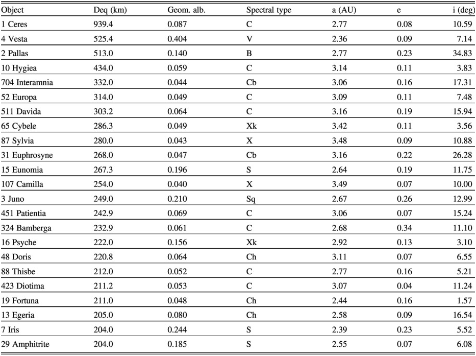
Table 1.1 Volume equivalent diameter (Deq), geometric albedo, spectral type following the Bus-DeMeo taxonomy, semi-major axis (a), eccentricity (e), and inclination (i) for the largest (D > 200 km) Main Belt asteroids listed according to decreasing values of their size.
The albedo and diameter values represent the averages of the values reported in Tedesco et al. (Reference Tedesco, Noah, Noah and Price2002), Usui et al. (Reference Usui, Hasegawa, Ootsubo and Onaka2011), and Masiero et al. (Reference Masiero, Mainzer and Grav2011, Reference Masiero, Grav and Mainzer2014). Spectral types were retrieved from Bus and Binzel (Reference Bus and Binzel2002), Lazzaro et al. (Reference Lazzaro, Angeli and Carvano2004), and DeMeo et al. (Reference DeMeo, Alexander, Walsh, Chapman, Binzel, Michel, DeMeo and Bottke2009)
| Object | Deq (km) | Geom. alb. | Spectral type | a (AU) | e | i (deg) |
|---|---|---|---|---|---|---|
| 1 Ceres | 939.4 | 0.087 | C | 2.77 | 0.08 | 10.59 |
| 4 Vesta | 525.4 | 0.404 | V | 2.36 | 0.09 | 7.14 |
| 2 Pallas | 513.0 | 0.140 | B | 2.77 | 0.23 | 34.83 |
| 10 Hygiea | 434.0 | 0.059 | C | 3.14 | 0.11 | 3.83 |
| 704 Interamnia | 332.0 | 0.044 | Cb | 3.06 | 0.16 | 17.31 |
| 52 Europa | 314.0 | 0.049 | C | 3.09 | 0.11 | 7.48 |
| 511 Davida | 303.2 | 0.064 | C | 3.16 | 0.19 | 15.94 |
| 65 Cybele | 286.3 | 0.049 | Xk | 3.42 | 0.11 | 3.56 |
| 87 Sylvia | 280.0 | 0.043 | X | 3.48 | 0.09 | 10.88 |
| 31 Euphrosyne | 268.0 | 0.047 | Cb | 3.16 | 0.22 | 26.28 |
| 15 Eunomia | 267.3 | 0.196 | S | 2.64 | 0.19 | 11.75 |
| 107 Camilla | 254.0 | 0.040 | X | 3.49 | 0.07 | 10.00 |
| 3 Juno | 249.0 | 0.210 | Sq | 2.67 | 0.26 | 12.99 |
| 451 Patientia | 242.9 | 0.069 | C | 3.06 | 0.07 | 15.24 |
| 324 Bamberga | 232.9 | 0.061 | C | 2.68 | 0.34 | 11.10 |
| 16 Psyche | 222.0 | 0.156 | Xk | 2.92 | 0.13 | 3.10 |
| 48 Doris | 220.8 | 0.064 | Ch | 3.11 | 0.07 | 6.55 |
| 88 Thisbe | 212.0 | 0.052 | C | 2.77 | 0.16 | 5.21 |
| 423 Diotima | 211.2 | 0.053 | C | 3.07 | 0.04 | 11.24 |
| 19 Fortuna | 211.0 | 0.048 | Ch | 2.44 | 0.16 | 1.57 |
| 13 Egeria | 205.0 | 0.080 | Ch | 2.58 | 0.09 | 16.54 |
| 7 Iris | 204.0 | 0.244 | S | 2.39 | 0.23 | 5.52 |
| 29 Amphitrite | 204.0 | 0.185 | S | 2.55 | 0.07 | 6.08 |
Table 1.2 Volume equivalent diameter (Deq), geometric albedo, spectral type following the Bus-DeMeo taxonomy, semi-major axis (a), eccentricity (e), and inclination (i) for the largest (D > 100 km) Main Belt asteroids.
The albedo and diameter values represent the averages of the values reported in Tedesco et al. (Reference Tedesco, Noah, Noah and Price2002), Masiero et al. (Reference Masiero, Mainzer and Grav2011, Reference Masiero, Grav and Mainzer2014), and Usui et al. (Reference Usui, Hasegawa, Ootsubo and Onaka2011). Spectral types were retrieved from Bus and Binzel (Reference Bus and Binzel2002), Lazzaro et al. (Reference Lazzaro, Angeli and Carvano2004), and DeMeo et al. (Reference DeMeo, Alexander, Walsh, Chapman, Binzel, Michel, DeMeo and Bottke2009). The spectral type in braces was determined using the Bus and Binzel (Reference Bus and Binzel2002) taxonomy
| Object | Deq (km) | Geom. Alb. | Spectral type | a (AU) | e | i (deg) |
|---|---|---|---|---|---|---|
| 1 Ceres | 939.4 | 0.087 | C | 2.77 | 0.08 | 10.59 |
| 2 Pallas | 513.0 | 0.140 | B | 2.77 | 0.23 | 34.83 |
| 3 Juno | 249.0 | 0.210 | Sq | 2.67 | 0.26 | 12.99 |
| 4 Vesta | 525.4 | 0.404 | V | 2.36 | 0.09 | 7.14 |
| 5 Astraea | 114.0 | 0.236 | S | 2.57 | 0.19 | 5.37 |
| 6 Hebe | 196.0 | 0.220 | S | 2.43 | 0.20 | 14.75 |
| 7 Iris | 204.0 | 0.244 | S | 2.39 | 0.23 | 5.52 |
| 8 Flora | 140.0 | 0.226 | Sw | 2.20 | 0.16 | 5.89 |
| 9 Metis | 168.0 | 0.189 | K | 2.39 | 0.12 | 5.58 |
| 10 Hygiea | 434.0 | 0.059 | C | 3.14 | 0.11 | 3.83 |
| 11 Parthenope | 154.5 | 0.186 | Sq | 2.45 | 0.10 | 4.63 |
| 12 Victoria | 129.7 | 0.134 | L | 2.33 | 0.22 | 8.37 |
| 13 Egeria | 205.0 | 0.080 | Ch | 2.58 | 0.09 | 16.54 |
| 14 Irene | 149.7 | 0.239 | S | 2.59 | 0.17 | 9.12 |
| 15 Eunomia | 267.3 | 0.196 | S | 2.64 | 0.19 | 11.75 |
| 16 Psyche | 222.0 | 0.156 | Xk | 2.92 | 0.13 | 3.10 |
| 18 Melpomene | 146.0 | 0.190 | S | 2.30 | 0.22 | 10.13 |
| 19 Fortuna | 211.0 | 0.048 | Ch | 2.44 | 0.16 | 1.57 |
| 20 Massalia | 140.8 | 0.229 | S | 2.41 | 0.14 | 0.71 |
| 21 Lutetia | 98.0 | 0.184 | Xc | 2.44 | 0.16 | 3.06 |
| 22 Kalliope | 161.0 | 0.171 | X | 2.91 | 0.10 | 13.72 |
| 23 Thalia | 105.1 | 0.270 | S | 2.63 | 0.24 | 10.11 |
| 24 Themis | 189.6 | 0.074 | C | 3.14 | 0.13 | 0.75 |
| 27 Euterpe | 113.9 | 0.218 | S | 2.35 | 0.17 | 1.58 |
| 28 Bellona | 122.7 | 0.187 | S | 2.78 | 0.15 | 9.43 |
| 29 Amphitrite | 204.0 | 0.185 | S | 2.55 | 0.07 | 6.08 |
| 31 Euphrosyne | 268.0 | 0.047 | Cb | 3.16 | 0.22 | 26.28 |
| 34 Circe | 117.1 | 0.051 | Ch | 2.69 | 0.10 | 5.50 |
| 35 Leukothea | 104.1 | 0.066 | (C) | 2.99 | 0.23 | 7.94 |
| 36 Atalante | 111.5 | 0.060 | Ch | 2.75 | 0.30 | 18.43 |
| 37 Fides | 110.0 | 0.182 | S | 2.64 | 0.17 | 3.07 |
| 38 Leda | 116.1 | 0.063 | Cgh | 2.74 | 0.15 | 6.97 |
| 39 Laetitia | 164.0 | 0.238 | Sqw | 2.77 | 0.11 | 10.38 |
| 40 Harmonia | 116.7 | 0.209 | S | 2.27 | 0.05 | 4.26 |
| 41 Daphne | 187.0 | 0.055 | Ch | 2.76 | 0.28 | 15.79 |
| 42 Isis | 106.7 | 0.152 | K | 2.44 | 0.22 | 8.53 |
| 45 Eugenia | 186.0 | 0.051 | C | 2.72 | 0.08 | 6.60 |
| 46 Hestia | 126.0 | 0.051 | Xc | 2.53 | 0.17 | 2.34 |
| 47 Aglaja | 142.0 | 0.064 | C | 2.88 | 0.13 | 4.98 |
| 48 Doris | 220.8 | 0.064 | Ch | 3.11 | 0.07 | 6.55 |
| 49 Pales | 161.3 | 0.052 | Ch | 3.09 | 0.23 | 3.17 |
| 50 Virginia | 94.4 | 0.041 | Ch | 2.65 | 0.28 | 2.83 |
| 51 Nemausa | 144.0 | 0.078 | Cgh | 2.37 | 0.07 | 9.98 |
| 52 Europa | 314.0 | 0.049 | C | 3.09 | 0.11 | 7.48 |
| 53 Kalypso | 110.7 | 0.044 | Ch | 2.62 | 0.21 | 5.17 |
| 54 Alexandra | 143.0 | 0.066 | Cgh | 2.71 | 0.20 | 11.80 |
| 56 Melete | 120.0 | 0.060 | Xk | 2.60 | 0.24 | 8.07 |
| 57 Mnemosyne | 114.5 | 0.209 | S | 3.15 | 0.12 | 15.22 |
| 59 Elpis | 168.0 | 0.043 | C | 2.71 | 0.12 | 8.63 |
| 62 Erato | 97.0 | 0.063 | B | 3.13 | 0.17 | 2.23 |
| 65 Cybele | 286.3 | 0.049 | Xk | 3.43 | 0.11 | 3.56 |
| 68 Leto | 127.2 | 0.215 | S | 2.78 | 0.19 | 7.97 |
| 69 Hesperia | 134.8 | 0.150 | Xk | 2.98 | 0.17 | 8.59 |
| 70 Panopaea | 137.1 | 0.050 | Cgh | 2.61 | 0.18 | 11.59 |
| 74 Galatea | 122.6 | 0.042 | (C) | 2.78 | 0.24 | 4.08 |
| 76 Freia | 173.1 | 0.042 | C | 3.41 | 0.16 | 2.12 |
| 78 Diana | 145.5 | 0.051 | Ch | 2.62 | 0.21 | 8.70 |
| 81 Terpsichore | 124.0 | 0.042 | C | 2.86 | 0.21 | 7.80 |
| 85 Io | 165.0 | 0.054 | C | 2.66 | 0.19 | 11.96 |
| 86 Semele | 119.2 | 0.049 | Cgh | 3.11 | 0.21 | 4.82 |
| 87 Sylvia | 280.0 | 0.043 | X | 3.48 | 0.09 | 10.88 |
| 88 Thisbe | 212.0 | 0.052 | C | 2.77 | 0.16 | 5.21 |
| 89 Julia | 140.0 | 0.172 | S | 2.55 | 0.18 | 16.14 |
| 90 Antiope | 108.0 | 0.087 | C | 3.16 | 0.16 | 2.21 |
| 91 Aegina | 109.0 | 0.042 | Ch | 2.59 | 0.11 | 2.11 |
| 92 Undina | 121.0 | 0.280 | Xk | 3.19 | 0.10 | 9.93 |
| 93 Minerva | 159.0 | 0.048 | C | 2.76 | 0.14 | 8.56 |
| 94 Aurora | 199.0 | 0.041 | C | 3.16 | 0.09 | 7.97 |
| 95 Arethusa | 144.5 | 0.062 | Ch | 3.07 | 0.15 | 13.00 |
| 96 Aegle | 172.9 | 0.051 | T | 3.05 | 0.14 | 15.97 |
| 98 Ianthe | 109.8 | 0.043 | (Ch) | 2.69 | 0.19 | 15.58 |
| 104 Klymene | 127.8 | 0.054 | Ch | 3.15 | 0.16 | 2.79 |
| 105 Artemis | 121.0 | 0.045 | Ch | 2.37 | 0.18 | 21.44 |
| 106 Dione | 174.7 | 0.067 | Cgh | 3.18 | 0.17 | 4.60 |
| 107 Camilla | 254.0 | 0.040 | X | 3.49 | 0.07 | 10.00 |
| 111 Ate | 144.9 | 0.053 | Ch | 2.59 | 0.10 | 4.93 |
| 114 Kassandra | 99.0 | 0.090 | K | 2.68 | 0.14 | 4.93 |
| 117 Lomia | 158.6 | 0.048 | (X) | 2.99 | 0.03 | 14.90 |
| 120 Lachesis | 170.2 | 0.050 | C | 3.12 | 0.06 | 6.95 |
| 121 Hermione | 187.0 | 0.061 | Ch | 3.45 | 0.13 | 7.60 |
| 127 Johanna | 121.7 | 0.053 | Ch | 2.76 | 0.07 | 8.24 |
| 128 Nemesis | 185.4 | 0.053 | C | 2.75 | 0.12 | 6.25 |
| 129 Antigone | 126.0 | 0.147 | Xk | 2.88 | 0.21 | 12.23 |
| 130 Elektra | 199.0 | 0.064 | Ch | 3.12 | 0.21 | 22.86 |
| 134 Sophrosyne | 113.3 | 0.045 | (Ch) | 2.56 | 0.12 | 11.60 |
| 137 Meliboea | 147.8 | 0.049 | (C) | 3.12 | 0.22 | 13.41 |
| 139 Juewa | 167.2 | 0.047 | (X) | 2.78 | 0.18 | 10.91 |
| 140 Siwa | 114.0 | 0.063 | Xc | 2.73 | 0.22 | 3.19 |
| 141 Lumen | 136.4 | 0.050 | Ch | 2.67 | 0.21 | 11.89 |
| 144 Vibilia | 141.0 | 0.051 | Ch | 2.66 | 0.24 | 4.81 |
| 145 Adeona | 150.1 | 0.044 | Ch | 2.67 | 0.15 | 12.64 |
| 146 Lucina | 134.5 | 0.052 | Ch | 2.72 | 0.07 | 13.10 |
| 147 Protogeneia | 121.8 | 0.062 | C | 3.14 | 0.03 | 1.93 |
| 150 Nuwa | 145.5 | 0.043 | C | 2.98 | 0.13 | 2.19 |
| 153 Hilda | 186.6 | 0.055 | X | 3.97 | 0.14 | 7.83 |
| 154 Bertha | 187.0 | 0.047 | (C) | 3.20 | 0.08 | 20.98 |
| 156 Xanthippe | 113.6 | 0.048 | Ch | 2.73 | 0.23 | 9.78 |
| 159 Aemilia | 130.0 | 0.059 | Ch | 3.10 | 0.11 | 6.13 |
| 162 Laurentia | 98.6 | 0.055 | (Ch) | 3.02 | 0.18 | 6.10 |
| 164 Eva | 107.7 | 0.039 | (X) | 2.63 | 0.34 | 24.47 |
| 165 Loreley | 173.0 | 0.045 | (Cb) | 3.12 | 0.08 | 11.22 |
| 168 Sibylla | 148.8 | 0.054 | (Ch) | 3.37 | 0.07 | 4.64 |
| 171 Ophelia | 110.6 | 0.071 | (Cb) | 3.13 | 0.13 | 2.55 |
| 173 Ino | 152.6 | 0.069 | Xk | 2.74 | 0.21 | 14.21 |
| 175 Andromache | 110.8 | 0.071 | Cg | 3.18 | 0.23 | 3.22 |
| 176 Iduna | 124.3 | 0.080 | (Ch) | 3.19 | 0.17 | 22.59 |
| 181 Eucharis | 118.2 | 0.095 | Xk | 3.13 | 0.20 | 18.89 |
| 185 Eunike | 168.2 | 0.057 | C | 2.74 | 0.13 | 23.22 |
| 187 Lamberta | 131.8 | 0.059 | Ch | 2.73 | 0.24 | 10.59 |
| 190 Ismene | 197.3 | 0.043 | X | 4.00 | 0.17 | 6.16 |
| 191 Kolga | 102.3 | 0.040 | Cb | 2.89 | 0.09 | 11.51 |
| 194 Prokne | 172.6 | 0.050 | Ch | 2.62 | 0.24 | 18.49 |
| 196 Philomela | 148.8 | 0.195 | (S) | 3.11 | 0.02 | 7.26 |
| 200 Dynamene | 133.4 | 0.050 | (Ch) | 2.74 | 0.13 | 6.90 |
| 203 Pompeja | 111.3 | 0.045 | (C-complex) | 2.74 | 0.06 | 3.18 |
| 206 Hersilia | 99.3 | 0.062 | (C) | 2.74 | 0.04 | 3.78 |
| 209 Dido | 138.2 | 0.049 | (Xc) | 3.14 | 0.06 | 7.17 |
| 210 Isabella | 85.8 | 0.048 | Cb | 2.72 | 0.12 | 5.26 |
| 211 Isolda | 149.2 | 0.056 | Ch | 3.04 | 0.16 | 3.89 |
| 212 Medea | 150.0 | 0.039 | X | 3.12 | 0.11 | 4.26 |
| 216 Kleopatra | 121.0 | 0.145 | Xe | 2.80 | 0.25 | 13.10 |
| 221 Eos | 105.6 | 0.139 | K | 3.01 | 0.10 | 10.88 |
| 225 Henrietta | 119.3 | 0.042 | (B) | 3.39 | 0.26 | 20.87 |
| 227 Philosophia | 97.6 | 0.056 | (X) | 3.17 | 0.19 | 9.11 |
| 229 Adelinda | 104.2 | 0.037 | X | 3.42 | 0.14 | 2.08 |
| 230 Athamantis | 112.0 | 0.163 | S | 2.38 | 0.06 | 9.44 |
| 233 Asterope | 106.0 | 0.157 | Xk | 2.66 | 0.10 | 7.69 |
| 238 Hypatia | 151.4 | 0.042 | (Ch) | 2.91 | 0.09 | 12.39 |
| 241 Germania | 178.7 | 0.052 | C | 3.05 | 0.10 | 5.51 |
| 247 Eukrate | 147.0 | 0.051 | (Xc) | 2.74 | 0.24 | 24.99 |
| 250 Bettina | 111.0 | 0.137 | Xk | 3.15 | 0.13 | 12.81 |
| 259 Aletheia | 185.3 | 0.041 | (X) | 3.13 | 0.13 | 10.82 |
| 266 Aline | 112.1 | 0.048 | Ch | 2.80 | 0.16 | 13.40 |
| 268 Adorea | 148.9 | 0.040 | X | 3.09 | 0.14 | 2.44 |
| 275 Sapientia | 110.9 | 0.042 | C | 2.77 | 0.16 | 4.76 |
| 276 Adelheid | 123.9 | 0.046 | X | 3.12 | 0.07 | 21.62 |
| 279 Thule | 124.9 | 0.043 | D | 4.28 | 0.01 | 2.34 |
| 283 Emma | 142.0 | 0.032 | C | 3.05 | 0.15 | 7.99 |
| 286 Iclea | 103.9 | 0.043 | (Ch) | 3.19 | 0.03 | 17.90 |
| 303 Josephina | 103.4 | 0.052 | (Ch) | 3.12 | 0.06 | 6.87 |
| 308 Polyxo | 147.3 | 0.045 | T | 2.75 | 0.04 | 4.36 |
| 324 Bamberga | 232.9 | 0.061 | C | 2.68 | 0.34 | 11.10 |
| 328 Gudrun | 120.1 | 0.045 | C/Cb | 3.11 | 0.11 | 16.12 |
| 334 Chicago | 182.7 | 0.050 | C | 3.90 | 0.02 | 4.64 |
| 344 Desiderata | 133.9 | 0.058 | Xk | 2.60 | 0.32 | 18.35 |
| 345 Tercidina | 101.5 | 0.058 | Ch | 2.33 | 0.06 | 9.75 |
| 349 Dembowska | 174.4 | 0.280 | R | 2.93 | 0.09 | 8.25 |
| 350 Ornamenta | 114.3 | 0.063 | (Ch) | 3.11 | 0.16 | 24.91 |
| 354 Eleonora | 159.9 | 0.187 | A | 2.80 | 0.12 | 18.40 |
| 356 Liguria | 134.2 | 0.051 | Ch | 2.76 | 0.24 | 8.22 |
| 357 Ninina | 104.6 | 0.053 | (B) | 3.15 | 0.07 | 15.08 |
| 360 Carlova | 135.0 | 0.039 | (C) | 3.00 | 0.18 | 11.70 |
| 361 Bononia | 150.5 | 0.041 | D | 3.96 | 0.21 | 12.62 |
| 365 Corduba | 101.6 | 0.037 | (C) | 2.80 | 0.16 | 12.78 |
| 372 Palma | 192.6 | 0.064 | (B) | 3.15 | 0.26 | 23.83 |
| 373 Melusina | 98.7 | 0.042 | (Ch) | 3.12 | 0.14 | 15.43 |
| 375 Ursula | 193.6 | 0.049 | C | 3.12 | 0.11 | 15.94 |
| 381 Myrrha | 127.6 | 0.055 | (Cb) | 3.22 | 0.09 | 12.53 |
| 386 Siegena | 167.0 | 0.053 | (C) | 2.90 | 0.17 | 20.26 |
| 387 Aquitania | 97.0 | 0.171 | L | 2.74 | 0.24 | 18.13 |
| 388 Charybdis | 122.2 | 0.044 | (C) | 3.01 | 0.06 | 6.44 |
| 393 Lampetia | 121.9 | 0.064 | (Xc) | 2.78 | 0.33 | 14.88 |
| 404 Arsinoe | 98.0 | 0.047 | (Ch) | 2.59 | 0.20 | 14.11 |
| 405 Thia | 124.4 | 0.048 | Ch | 2.58 | 0.24 | 11.95 |
| 409 Aspasia | 164.0 | 0.060 | Xc | 2.58 | 0.07 | 11.26 |
| 410 Chloris | 116.6 | 0.058 | (Ch) | 2.73 | 0.24 | 10.96 |
| 412 Elisabetha | 100.6 | 0.043 | (C) | 2.76 | 0.04 | 13.78 |
| 419 Aurelia | 122.5 | 0.043 | C | 2.60 | 0.25 | 3.93 |
| 420 Bertholda | 148.7 | 0.038 | D | 3.41 | 0.03 | 6.69 |
| 423 Diotima | 211.2 | 0.053 | C | 3.07 | 0.04 | 11.24 |
| 426 Hippo | 123.0 | 0.051 | B | 2.89 | 0.10 | 19.48 |
| 444 Gyptis | 165.6 | 0.047 | C | 2.77 | 0.18 | 10.28 |
| 445 Edna | 97.6 | 0.037 | (Ch) | 3.20 | 0.19 | 21.38 |
| 451 Patientia | 242.9 | 0.069 | C | 3.06 | 0.07 | 15.24 |
| 455 Bruchsalia | 98.5 | 0.052 | (Xk) | 2.66 | 0.29 | 12.02 |
| 466 Tisiphone | 111.0 | 0.072 | (Ch) | 3.35 | 0.09 | 19.11 |
| 469 Argentina | 127.4 | 0.039 | (Xk) | 3.18 | 0.16 | 11.59 |
| 471 Papagena | 132.0 | 0.232 | Sq | 2.89 | 0.23 | 14.98 |
| 476 Hedwig | 124.5 | 0.045 | Xk | 2.65 | 0.07 | 10.94 |
| 481 Emita | 112.5 | 0.047 | (Ch) | 2.74 | 0.16 | 9.84 |
| 488 Kreusa | 161.4 | 0.052 | (Ch) | 3.17 | 0.16 | 11.52 |
| 489 Comacina | 138.8 | 0.044 | (X) | 3.15 | 0.04 | 13.00 |
| 490 Veritas | 114.5 | 0.064 | Ch | 3.17 | 0.10 | 9.28 |
| 491 Carina | 99.1 | 0.063 | (C) | 3.19 | 0.09 | 18.87 |
| 505 Cava | 102.8 | 0.060 | Xk | 2.68 | 0.25 | 9.84 |
| 506 Marion | 108.0 | 0.045 | (X) | 3.04 | 0.15 | 17.00 |
| 508 Princetonia | 134.9 | 0.050 | (X) | 3.16 | 0.01 | 13.36 |
| 511 Davida | 303.2 | 0.064 | C | 3.16 | 0.19 | 15.94 |
| 514 Armida | 105.6 | 0.040 | (Xe) | 3.05 | 0.04 | 3.88 |
| 517 Edith | 96.3 | 0.037 | C | 3.16 | 0.18 | 3.19 |
| 521 Brixia | 118.9 | 0.060 | Ch | 2.74 | 0.28 | 10.60 |
| 522 Helga | 97.2 | 0.044 | (X) | 3.63 | 0.08 | 4.44 |
| 532 Herculina | 191.0 | 0.211 | S | 2.77 | 0.18 | 16.31 |
| 536 Merapi | 159.5 | 0.042 | Xk | 3.50 | 0.09 | 19.43 |
| 545 Messalina | 112.2 | 0.042 | (Cb) | 3.21 | 0.17 | 11.12 |
| 554 Peraga | 102.9 | 0.039 | Ch | 2.38 | 0.15 | 2.94 |
| 566 Stereoskopia | 167.0 | 0.042 | (X) | 3.38 | 0.11 | 4.90 |
| 570 Kythera | 102.4 | 0.051 | D | 3.42 | 0.12 | 1.79 |
| 595 Polyxena | 110.6 | 0.091 | (T) | 3.21 | 0.06 | 17.82 |
| 596 Scheila | 114.3 | 0.038 | T | 2.93 | 0.16 | 14.66 |
| 602 Marianna | 128.9 | 0.051 | (Ch) | 3.09 | 0.25 | 15.08 |
| 618 Elfriede | 133.6 | 0.050 | (C) | 3.19 | 0.07 | 17.04 |
| 635 Vundtia | 99.0 | 0.045 | (B) | 3.14 | 0.08 | 11.03 |
| 654 Zelinda | 128.3 | 0.042 | (Ch) | 2.30 | 0.23 | 18.13 |
| 683 Lanzia | 103.0 | 0.108 | (C) | 3.12 | 0.06 | 18.51 |
| 690 Wratislavia | 157.9 | 0.044 | (B) | 3.14 | 0.18 | 11.27 |
| 694 Ekard | 105.3 | 0.037 | (Ch) | 2.67 | 0.32 | 15.84 |
| 702 Alauda | 195.0 | 0.056 | C | 3.19 | 0.02 | 20.61 |
| 704 Interamnia | 332.0 | 0.044 | Cb | 3.06 | 0.16 | 17.31 |
| 705 Erminia | 137.4 | 0.042 | (C) | 2.92 | 0.05 | 25.04 |
| 712 Boliviana | 127.4 | 0.049 | (X) | 2.58 | 0.19 | 12.76 |
| 713 Luscinia | 101.8 | 0.044 | (C) | 3.39 | 0.17 | 10.36 |
| 733 Mocia | 102.6 | 0.041 | (X) | 3.40 | 0.06 | 20.26 |
| 739 Mandeville | 111.2 | 0.054 | Xc | 2.74 | 0.14 | 20.66 |
| 747 Winchester | 178.0 | 0.048 | (C) | 3.00 | 0.34 | 18.16 |
| 748 Simeisa | 106.6 | 0.039 | (T) | 3.96 | 0.19 | 2.26 |
| 751 Faina | 111.9 | 0.050 | (Ch) | 2.55 | 0.15 | 15.61 |
| 762 Pulcova | 149.0 | 0.055 | C | 3.16 | 0.10 | 13.09 |
| 769 Tatjana | 106.3 | 0.044 | (C-complex) | 3.17 | 0.19 | 7.37 |
| 772 Tanete | 130.6 | 0.050 | C | 3.00 | 0.09 | 28.86 |
| 776 Berbericia | 155.6 | 0.063 | Cgh | 2.93 | 0.16 | 18.25 |
| 780 Armenia | 99.7 | 0.045 | (C) | 3.11 | 0.10 | 19.09 |
| 786 Bredichina | 101.3 | 0.060 | (X/Xc) | 3.17 | 0.16 | 14.55 |
| 788 Hohensteina | 119.2 | 0.060 | (Ch) | 3.12 | 0.13 | 14.34 |
| 790 Pretoria | 159.1 | 0.045 | (X) | 3.41 | 0.15 | 20.53 |
| 804 Hispania | 158.8 | 0.052 | (C) | 2.84 | 0.14 | 15.36 |
| 814 Tauris | 111.0 | 0.045 | (C) | 3.15 | 0.31 | 21.83 |
| 895 Helio | 134.2 | 0.049 | (B) | 3.20 | 0.15 | 26.09 |
| 909 Ulla | 114.8 | 0.036 | X | 3.54 | 0.09 | 18.79 |
| 1015 Christa | 100.6 | 0.043 | (Xc) | 3.21 | 0.08 | 9.46 |
| 1021 Flammario | 101.0 | 0.045 | C | 2.74 | 0.28 | 15.87 |
| 1093 Freda | 112.2 | 0.043 | (Cb) | 3.13 | 0.27 | 25.21 |
| 1269 Rollandia | 108.2 | 0.045 | (D) | 3.91 | 0.10 | 2.76 |
Early photometric observations of these bodies were key in establishing the existence of a compositional gradient in the asteroid belt (Gradie & Tedesco, Reference Gradie and Tedesco1982), with S-types being located on average closer to the Sun than C-types and P-/D-types being the farthest from the Sun. On the basis of these observations, scenarios regarding the formation and dynamical evolution of the asteroid belt and that of the Solar System in general have been formulated (e.g., Gomes et al., Reference Gomes, Levison, Tsiganis and Morbidelli2005; Morbidelli et al., Reference Morbidelli, Bottke, Nesvorny and Levison2005; Tsiganis et al., Reference Tsiganis, Gomes, Morbidelli and Levison2005; Bottke et al., Reference Bottke, Nesvorny, Grimm, Morbidelli and O’Brien2006; Levison et al., Reference Levison, Bottke and Gounelle2009; Walsh et al., Reference Walsh, Morbidelli, Raymond, O’Brien and Mandell2011; Raymond & Izidoro, Reference Raymond and Izidoro2017). These dynamical models suggest that today’s asteroid belt may not only host objects that formed in situ, typically between 2.2 and 3.3 AU, but also bodies that were formed in the terrestrial planet region (Xe- and possibly S-types), in the giant planet region (Ch/Cgh- and B/C-types) as well as beyond Neptune (P/D-types). In a broad stroke, the idea that the asteroid belt is a condensed version of the primordial Solar System has progressively emerged. Notably, these observations along with those of more distant small bodies (giant planet trojans, trans-Neptunian objects) were instrumental in imposing giant planet migrations as a main step in the dynamical evolution of our Solar System. On the basis of these datasets, the idea of a static Solar System history has dramatically shifted to one of dynamic change and mixing (DeMeo & Carry, Reference DeMeo and Carry2014). See Part III of this book for more details on this topic.
The study of the largest Main Belt asteroids is not only important because of the clues it delivers regarding the formation and evolution of the belt itself but also because many of these bodies are likely “primordial” remnants of the early Solar System (Morbidelli et al., Reference Morbidelli, Bottke, Nesvorny and Levison2009), that is their internal structure has likely remained intact since their formation (they can be seen as the smallest protoplanets). Many of these bodies thus offer, similarly to Ceres and Vesta detailed in the present book, invaluable constraints regarding the processes of protoplanet formation over a wide range of heliocentric distances (assuming that the aforementioned migration theories are correct).
In the present chapter, we review the current knowledge regarding large (D ≳100 km) Main Belt asteroids derived from Earth-based spectroscopic and imaging observations with an emphasis on D > 200 km bodies including Ceres and Vesta. Our motivation is to provide a meaningful context for the two largest Main Belt asteroids visited by the Dawn mission (see Chapter 2) and to guide future in-situ investigations to the largest asteroids – that’s why small (D < 100 km) asteroids, which are essentially the leftover fragments of catastrophic collisions, are not discussed here.
1.2 Spectroscopic Observations of Large Main Belt Asteroids
Detailed reviews concerning the compositional interpretation of asteroid taxonomic types and their distribution across the Main Belt can be found in Burbine (Reference Burbine and Davis2014, Reference Burbine2016), DeMeo et al. (Reference DeMeo, Alexander, Walsh, Chapman, Binzel, Michel, DeMeo and Bottke2015), Reddy et al. (Reference Rivkin and Emery2015), Vernazza et al. (Reference Vernazza, Zanda, Nakamura, Michel, DeMeo and Bottke2015b), Vernazza and Beck (Reference Vernazza, Beck, Elkins-Tanton and Weiss2017), and Greenwood et al. (Reference Greenwood, Burbine and Franchi2020) and will not be repeated with the same level of detail in this chapter. Rather, we put the emphasis on the currently proposed connections between the various compositional classes present among the largest Main Belt asteroids and the two main classes of extra-terrestrial materials, namely meteorites and interplanetary dust particles (hereafter IDPs). The two largest asteroids, Vesta and Ceres, “heroes” of the present book, illustrate well the Main Belt paradox: some asteroids appear well sampled by meteorites (Vesta) whereas others don’t (Ceres). IDPs may be more appropriate analogues for these bodies. We first start by summarizing the results of Earth-based spectroscopic campaigns devoted to constrain the surface composition of Ceres and Vesta and then continue by summarizing current knowledge regarding the surface composition of D > 100 km asteroids.
1.2.1 Focus on Earth-based Spectroscopic Observations of Ceres and Vesta and Comparison to Dawn Measurements
1.2.1.1 (1) Ceres
In the 1970s, Ceres was identified as a carbonaceous chondrite-like asteroid based on a low albedo (∼0.05–0.06) (Veverka, Reference Veverka1970; Matson, Reference Matson1971; Bowell & Zellner, Reference Bowell, Zellner and Gehrels1973) and a relatively flat reflectance from 0.5 to 2.5 μm (Chapman et al., Reference Chapman, McCord and Johnson1973, Reference Chapman, Morrison and Zellner1975; Johnson & Fanale, Reference Johnson and Fanale1973; Johnson et al., Reference Johnson, Matson, Veeder and Loer1975). A few years later, a ∼3.1 μm absorption feature was discovered in its spectrum (Lebofsky, Reference Lebofsky1978; Lebofsky et al., Reference Lebofsky, Feierberg and Tokunaga1981) and was interpreted as indicative of the presence of hydrated clay minerals similar to those present in carbonaceous chondrites at the surface of Ceres. Subsequent work proposed ammoniated saponite (King et al., Reference King, Clark, Calvin, Sherman and Brown1992) and water ice (Vernazza et al., Reference Vernazza, Mothé-Diniz and Barucci2005) as the origin of this band. The presence of water ice in the subsurface of Ceres was predicted based on the detection of OH escaping from the north polar region (A’Hearn & Feldman, Reference A’Hearn and Feldman1992). Rivkin et al. (Reference Rivkin, Li and Milliken2006b) reported the presence of carbonates and iron-rich clays at the surface of Ceres based on spectroscopic measurements in the 2–4 μm range. This compositional interpretation was refined a few years later (Milliken & Rivkin, Reference Milliken and Rivkin2009) and an assemblage consisting of a mixture of hydroxide brucite, magnesium carbonates, and serpentines was proposed to explain Ceres’ spectral properties. Recent observations with the AKARI satellite have revealed the presence of an additional absorption band in the 2.5–3.5 μm range that is located at 2.73 μm (Usui et al., Reference Vernazza, Beck, Elkins-Tanton and Weiss2019), while also confirming the presence of a band at 3.06–3.08 μm (Usui et al., Reference Vernazza, Beck, Elkins-Tanton and Weiss2019). Measurements performed by the VIR instrument onboard the Dawn mission have shown that the ∼3.06 μm band assigned to ammoniated phyllosilicates by King et al. (Reference King, Clark, Calvin, Sherman and Brown1992) is the most plausible interpretation (De Sanctis et al., Reference De Sanctis, Ammannito and Raponi2015), while the assemblage with brucite was not confirmed. The VIR instrument has further revealed the presence of water ice (Combe et al., Reference Combe, McCord and Tosi2016), carbonates (De Sanctis et al., Reference De Sanctis, Raponi and Ammannito2016), organics (De Sanctis et al., Reference De Sanctis, Ammannito and McSween2017), and chloride salts (De Sanctis et al., Reference De Sanctis, Ammannito and Raponi2020) at the surface of Ceres. See Chapters 7 and 8 for more detail.
Notably, a “genetic” link between Ceres and carbonaceous chondrites available in our collections has progressively been questioned with time (Milliken & Rivkin, Reference Milliken and Rivkin2009; Rivkin et al., Reference Rivkin, Li and Milliken2011). First, the ∼3.06 μm band present in Ceres spectrum differs from what is seen in carbonaceous chondrite spectra. Second, the band depth of the 2.73 μm band is shallower than that of CM-like (Ch-/Cgh-type) asteroids (Figure 1.1; Usui et al., Reference Vernazza, Beck, Elkins-Tanton and Weiss2019). Third, Ceres’ spectrum possesses a broad absorption band centered on ∼1.2–1.3 μm that is not seen in spectra of aqueously altered carbonaceous chondrite (Figure 1.1). Vernazza et al. (Reference Vernazza, Marsset and Beck2015a) and Marsset et al. (Reference Marsset, Broz and Vernazza2016) have tentatively attributed this absorption band to amorphous silicates (mainly olivine), whereas Yang and Jewitt (Reference Yang, Hanus and Carry2010) proposed magnetite instead. Observations in the mid-infrared wavelength range have further reinforced the existence of compositional differences between Ceres and carbonaceous chondrite meteorites (Vernazza et al., Reference Vernazza, Beck, Elkins-Tanton and Weiss2017, Figure 1.2). They have further revealed the presence of anhydrous silicates at the surface of Ceres in addition to phyllosilicates and carbonates.

Figure 1.1 Sample of reflectance spectra of D > 100 km asteroids in visible to near-infrared wavelengths obtained with ground-based telescopes (Bus & Binzel, Reference Bus and Binzel2002; Hasegawa et al., Reference Hasegawa, Murakawa and Ishiguro2003, Reference Hasegawa, Kuroda, Yanagisawa and Usui2017; Hardersen et al., Reference Hardersen, Gaffey and Abel2004; Lazzaro et al., Reference Lazzaro, Angeli and Carvano2004; Rivkin et al., Reference Rivkin, McFadden, Binzel and Sykes2006a; DeMeo et al., Reference DeMeo, Alexander, Walsh, Chapman, Binzel, Michel, DeMeo and Bottke2009; Vernazza et al., Reference Vernazza, Zanda and Binzel2014; Binzel et al., Reference Binzel, DeMeo and Turtelboom2019; some spectra were also retrieved from the smass.mit.edu database) and the AKARI satellite (Usui et al., Reference Vernazza, Beck, Elkins-Tanton and Weiss2019) representative of the compositional diversity among these bodies. The asteroid spectral types are indicated in parentheses. Spectra of analogue meteorites are also shown next to each asteroid type (data are retrieved from the RELAB spectral database). The gray region denotes the asteroid types for which no clear meteoritic analogues exist.

Figure 1.2 Emissivity spectra of C- (top) and P/D-type asteroids (bottom) compared to meteorite and IDP spectra. The data were retrieved from Emery et al. (Reference Drake2006), Brunetto et al. (Reference Broz, Morbidelli and Bottke2011), Marchis et al. (Reference Marchi, Ermakov and Raymond2012), Merouane et al. (Reference Merouane, Djouadi and Le Sergeant d’Hendecourt2014), and Vernazza et al. (Reference Vernazza, Castillo-Rogez and Beck2017). Here, we illustrate the typical mismatch between carbonaceous chondrites and most C-, P-, and D-type asteroids (Vernazza et al., Reference Vernazza, Marsset and Beck2015a). IDPs instead appear as more convincing analogues for these objects.
1.2.1.2 (4) Vesta
It has been well known since the 1970s that Vesta possesses a high albedo (0.3–0.4) (e.g., Allen, Reference Allen1970; Cruikshank & Morrison, Reference Cruikshank and Morrison1973; Tedesco et al., Reference Tedesco, Noah, Noah and Price2002; Ryan & Woodward, Reference Ryan and Woodward2010; Usui et al., Reference Usui, Hasegawa, Ootsubo and Onaka2011; Hasegawa et al., Reference Hasegawa, Miyasaka and Tokimasa2014) and that its surface is basaltic in composition (McCord et al., Reference McCord, Adams and Johnson1970; Larson & Fink, Reference Larson and Fink1975; McFadden et al., Reference McFadden, McCord and Pieters1977). Vesta’s spectrum displays two diagnostic absorption bands centered at ∼0.9 µm and ∼2 µm which imply the presence of pyroxene at its surface. A comparison of these observations with laboratory measurements of meteorites has revealed a spectral similarity between Vesta and that of the howardite–eucrite–diogenite (HED) achondritic meteorites (e.g., McCord et al., Reference McCord, Adams and Johnson1970; Feierberg & Drake, Reference Feierberg and Drake1980; Feierberg et al., Reference Feierberg and Drake1980; Hiroi et al., Reference Hiroi, Pieters and Takeda1994), opening the possibility that Vesta could be the parent body of this meteorite group (e.g., Drake, Reference Drake2001). Spectroscopic observations in the 3-μm region have delivered contrasting results. Hasegawa et al. (Reference Hasegawa, Murakawa and Ishiguro2003) were the first to report the presence of a shallow 3-μm absorption that they interpreted either as contamination by CM-like impactors or solar wind implantation. These results were not confirmed by Vernazza et al. (Reference Vernazza, Mothé-Diniz and Barucci2005), whereas Rivkin et al. (Reference Rivkin, McFadden, Binzel and Sykes2006a) could not formally rule out a shallow (∼1%) absorption band. Finally, the presence of olivine has been reported at the surface of Vesta on the basis of spectral and color data (Binzel et al., Reference Binzel, Gaffey and Thomas1997; Gaffey, Reference Gaffey1997; Dotto et al., Reference Dotto, Müller and Barucci2000; Heras et al., Reference Heras, Morris, Vandenbussche, Müller, Sitko, Sprague and Lynch2000).
The heterogeneity of Vesta’s surface composition has been studied since the late 1970s (e.g., Blanco & Catalano, Reference Blanco and Catalano1979; Degewij et al., Reference De Sanctis, Ammannito and Capria1979; Binzel et al., Reference Binzel, Gaffey and Thomas1997; Gaffey, Reference Gaffey1997; Vernazza et al., Reference Vernazza, Mothé-Diniz and Barucci2005; Rivkin et al., Reference Rivkin, McFadden, Binzel and Sykes2006a; Carry et al., Reference Carry, Vernazza, Dumas and Fulchignoni2010c), revealing a non-uniform surface composition which was later confirmed by the data obtained by the Dawn spacecraft’s visible and infrared spectrometer (De Sanctis et al., Reference De Sanctis, Ammannito and Capria2012). The Dawn measurements have further confirmed that the mineralogy of Vesta is consistent with HED meteorites while also revealing the presence of olivine-rich areas in unexpected locations far from the Rheasilvia impact basin (Ammannito et al., Reference Ammannito, DeSanctis and Ciarniello2013). For a detailed discussion see Chapter 3.
The primordial Vesta material is no longer found on Vesta alone but also among its family members. Early dynamical studies have suggested the existence of a Vesta dynamical family (Williams, Reference Williams and Gehrels1979; Zappalá et al., Reference Zappalà, Cellino, Farinella and Knežević1990). Follow-up spectroscopic observations at visible wavelengths have confirmed the existence of such a family, revealing 20 small (diameters <10 kilometers) main-belt asteroids with optical reflectance spectral features similar to those of Vesta and eucrite and diogenite meteorites (Binzel & Xu, Reference Binzel, DeMeo and Turtelboom1993). Since then, more than 15,000 objects have been identified as likely Vesta family members (Nesvorny, Reference Nesvorny2015), and several of these candidates have been confirmed via spectroscopic observations (e.g., Hardersen et al., Reference Hardersen, Reddy, Roberts and Mainzer2014, Reference Hargrove, Emery, Campins and Kelley2015; Fulvio et al., Reference Fulvio, Ieva and Perna2018). We recall here that the term “Vestoid” is usually employed to designate a member of the Vesta family in the literature. Whereas the Vestoids are all located in Vesta’s vicinity, between 2.1 and 2.5 AU, some V-types (see Tholen & Barucci, Reference Tholen, Barucci, Binzel, Gehrels and Matthews1989; Bus & Binzel, Reference Bus and Binzel2002; DeMeo et al., Reference DeMeo, Alexander, Walsh, Chapman, Binzel, Michel, DeMeo and Bottke2009 for a definition of asteroid taxonomies) have also been discovered in the near-Earth space (Cruikshank et al., Reference Cruikshank, Tholen, Hartmann, Bell and Brown1991; Binzel et al., Reference Binzel, Rivkin and Stuart2004, Reference Binzel, DeMeo and Turtelboom2019; Thomas et al., Reference Thomas, Emery and Trilling2014) as well as in the middle and the outer belt (e.g., Lazzaro et al., Reference Lazzaro, Michtchenko and Carvano2000; Roig & Gil-Hutton, Reference Roig and Gil-Hutton2006; Moskovitz et al., Reference Moskovitz, Jedicke and Gaidos2008; Roig et al., Reference Roig, Nesvorný, Gil-Hutton and Lazzaro2008; Hardersen et al., Reference Hardersen, Reddy and Cloutis2018). Whereas V-type NEAs might have originated in the Vesta family and escaped the inner belt via the ν6 and 3:1 resonances, it is unlikely to be the case for most middle and outer Main Belt V-types (e.g., Fulvio et al., Reference Fulvio, Ieva and Perna2018; Hardersen et al., Reference Hardersen, Reddy and Cloutis2018). (1459) Magnya, in particular, located at 3.15 AU, is unlikely to be from Vesta (Lazzaro et al., Reference Lazzaro, Michtchenko and Carvano2000; Hardersen et al., Reference Hardersen, Gaffey and Abel2004). These results imply that the basaltic population present in the asteroid belt is not limited to Vesta and its family. Rather, it encompasses a larger number of bodies.
1.2.2 Extra-Terrestrial Analogues of D > 100 km Main Belt Asteroids
1.2.2.1 Asteroid Types with Plausible Meteoritic Analogues
Meteorites, which are mostly fragments of Main Belt asteroids, have played a key role in our understanding of the surface composition of asteroids and their distribution across the Main Belt. Their spectral properties have been measured in laboratories over an extended wavelength range (from the visible to the mid-infrared; e.g. Gaffey, Reference Gaffey1976; Cloutis et al., Reference Cloutis, Hardensen and Bish2010, Reference Cloutis, Hiroi, Gaffey, Alexander and Mann2011, Reference Cloutis, Hudon, Hiroi and Gaffey2012, Reference Cloutis, Izawa and Pompilio2013; Beck et al., Reference Beck, Garenne and Quirico2014) and used for direct comparison with those acquired for asteroids via telescopic observations (see Burbine, Reference Burbine and Davis2014, Reference Burbine2016; DeMeo et al., Reference DeMeo, Alexander, Walsh, Chapman, Binzel, Michel, DeMeo and Bottke2015; Reddy et al., Reference Rivkin and Emery2015; Vernazza & Beck, Reference Vernazza, Beck, Elkins-Tanton and Weiss2017, and references therein). Because most minerals present in meteorites possess diagnostic features either in the near- or mid-infrared and because quality measurements in these ranges became available for a large number of asteroids in the late 1990s, we can say that the Golden Age of asteroid compositional studies really started toward the end of the second millennium.
About 60% of the spectral types defined by DeMeo et al. (Reference DeMeo, Alexander, Walsh, Chapman, Binzel, Michel, DeMeo and Bottke2009) (A, Cgh, Ch, K, Q, R, S, Sa, Sq, Sr, Sv, V, and some X, Xc, and Xk types) can be linked to (or entirely defined by) a given meteorite class. Hereafter, we make a brief summary of these associations as well as a review of the spectroscopic observations of D > 100 km bodies belonging to these classes:
A-type asteroids mostly comprise the parent bodies of differentiated meteorites such as brachinites and pallasites, and possibly those of the undifferentiated R chondrite meteorites (Sunshine et al., Reference Sunshine, Bus, Corrigan, McCoy and Burbine2007). (354) Eleonora is the only D > 100 km A-type asteroid and it contains more than 80% of the mass of all A-type bodies (DeMeo et al., Reference DeMeo, Polihook and Carry2019). Its composition is compatible with that of differentiated meteorites (Sunshine et al., Reference Sunshine, Bus, Corrigan, McCoy and Burbine2007).
Ch- and Cgh-type asteroids comprise the parent bodies of CM chondrites (Vilas & Gaffey, Reference Viikinkoski, Vernazza and Hanus1989; Vernazza et al., Reference Vernazza, Marsset and Beck2016, and references therein). The Main Belt contains 61 CM-like bodies with diameters greater than 100 km. The analysis of the visible and near-infrared spectral properties of 34 of these bodies were reported by Vernazza et al. (Reference Vernazza, Marsset and Beck2016). They showed that the spectral variation observed among these bodies is essentially due to variations in the average regolith grain size. In addition, they showed that the spectral properties of the vast majority (unheated) of CM chondrites resemble both the surfaces and the interiors of CM-like bodies, implying a “low” temperature (<300°C) thermal evolution of the CM parent body(ies). It follows that an impact origin is the likely explanation for the existence of heated CM chondrites.
K-type asteroids comprise the parent bodies of CV, CO, CR, and CK meteorites (e.g. Bell, Reference Bell1988; Burbine et al., Reference Burbine, Binzel, Bus and Clark2001; Clark et al., Reference Clark, Ockert-Bell and Cloutis2009). The four D > 100 km K-type asteroids are (9) Mertis, (42) Isis, (114) Kassandra, and (221) Eos, with Eos being the largest remnant of a large outer Main Belt family (e.g., Broz et al., Reference Burbine and Davis2013).
The R-type class counts only one object so far, (349) Dembowska. Of interest to the present chapter, this object is a D > 100 km body and its meteoritic analogues may comprise both the lodranite and acapulcoite achondritic meteorites. While (349) Dembowska’s visible and near infrared spectrum appear very similar to those of H-like S-type asteroids (Vernazza et al., Reference Vernazza, Marsset and Beck2015a), the depth of its 1- and 2-μm bands is much larger than that observed in S-type spectra (see Figure 1.1). As noticed by Vernazza et al. (Reference Vernazza, Marsset and Beck2015a), both lodranites and acapulcoites have spectral properties and ol/(ol + low Ca-px) ratios that are very similar to those of ordinary chondrites and H chondrites in particular. Yet, given their lower iron content, the depth of their 1- and 2-μm bands are larger than those of H chondrites (see Figure 1.1), making them plausible analogues for a body such as (349) Dembowska.
S-complex asteroids (Q, S, Sa, Sq, Sr, Sv) comprise the parent bodies of the most common type of meteorites, namely ordinary chondrites (∼80% of the falls; see Vernazza et al., Reference Vernazza, Zanda, Nakamura, Michel, DeMeo and Bottke2015b for a detailed review on this topic), and also possibly those of some differentiated meteorites such as lodranites and acapulcoites (Vernazza et al., Reference Vernazza, Zanda, Nakamura, Michel, DeMeo and Bottke2015b). Vernazza et al. (Reference Vernazza, Zanda and Binzel2014) analyzed the visible and near-infrared spectral properties of nearly 100 S-type asteroids among which 23 bodies have diameters greater than 100 km (out of 24 in total). They found that the surface composition of these bodies is compatible with that of H, L, and LL ordinary chondrites, and that H-like bodies are located on average further from the sun than LL-like ones. This is somewhat counterintuitive given that H chondrites are more reduced than LL chondrites, suggesting a formation closer to the sun.
(4) Vesta is the only D > 100 km V-type, and its connection with HED meteorites has been described in Section 1.2.1.
X-complex asteroids (X, Xc, and Xk types) are representative of a great compositional diversity that largely exceeds (in terms of the number of compositional analogues) the number of taxonomic types. Their geometric albedos range from values below 0.05 to about 0.20. Notably, while some low albedo (<0.1) X-complex bodies likely comprise the parent bodies of rare types of meteorites such as Tagish Lake or CI chondrites, the remaining low albedo X-complex bodies appear unsampled by available meteorites in our collections (see Section 1.2.2.2). So far, there isn’t a single D > 100 low albedo X-complex asteroid that can be unambiguously linked to either the Tagish Lake meteorite or CI chondrites. Concerning the high albedo (>0.1) X-complex bodies, they likely comprise the parent bodies of (1) iron meteorites (e.g. Cloutis et al., Reference Cloutis, Gaffey, Smith and Lambert1990; Shepard et al., Reference Shepard, Taylor and Nolan2015, and references therein), (2) enstatite chondrites (ECs) and aubrites (e.g., Vernazza et al., Reference Vernazza, Brunetto and Binzel2009, Reference Vernazza, Carry and Vachier2011; Ockert-Bell et al., Reference Ockert-Bell, Clark and Shepard2010; Shepard et al., Reference Shepard, Taylor and Nolan2015), and (3) CB and CH chondrites (e.g., Hardersen et al., Reference Hardersen, Reddy and Cloutis2011; Shepard et al., Reference Shepard, Taylor and Nolan2015). The compositional interpretation of the visible and near-infrared spectral properties and/or the radar data for many D > 100 km X-complex asteroids can be found in Ockert-Bell et al. (Reference Ockert-Bell, Clark and Shepard2010), Hardersen et al. (Reference Hardersen, Reddy and Cloutis2011), Vernazza et al. (Reference Vernazza, Brunetto and Binzel2009, Reference Vernazza, Carry and Vachier2011), and Shepard et al. (Reference Shepard, Taylor and Nolan2015).
1.2.2.2 Asteroid Types with No Clear Meteoritic Analogues
About 40% of the spectral types defined by DeMeo et al. (Reference DeMeo, Alexander, Walsh, Chapman, Binzel, Michel, DeMeo and Bottke2009) (B, C, Cb, Cg, D, L, O, T, Xe, Xn, and most low albedo X, Xc, and Xk types) cannot be unambiguously linked to (or entirely defined by) a given meteorite class (e.g., Sunshine et al., Reference Sunshine, Connolly and McCoy2008; Vernazza et al., Reference Vernazza, Marsset and Beck2015a, Reference Vernazza, Castillo-Rogez and Beck2017).
In a few cases, this may be due to the rarity of the spectral type with L, O, Xe, and Xn types representing less than ∼1% of the mass of the Main Belt (DeMeo & Carry, Reference DeMeo and Carry2013). As a matter of fact, our meteorite collections do certainly not sample every single Main Belt asteroid, and it may thus not be a surprise that some rare asteroid types are absent from our meteorite collections.
In most cases, however, the spectral mismatch between asteroid and meteorite spectra must be telling us something important about the nature of these unsampled yet abundant asteroid types (B, C, Cb, Cg, D, T, and low albedo X-, Xc-, and Xk-type asteroids represent at least 50% of the mass of the asteroid belt; DeMeo & Carry, Reference DeMeo and Carry2013). Notably, these asteroid types (particularly the B, C, Cb, and Cg types) comprise – similarly to S-types – a high number of large asteroid families such as the Hygiea, Themis, Euphrosyne, Nemesis, and Polana-Eulalia (Pinilla-Alonso et al., Reference Pinilla-Alonso, De Leon and Walsh2016) families (see Broz et al., Reference Burbine and Davis2013 and Nesvorny, Reference Nesvorny2015 for further information on asteroid families). Considering that asteroid families are a major source of meteorites (this is well supported by the connection between the Vesta family and the HED meteorites), we should be receiving plenty of fragments from these bodies. Yet, this seems not to be the case, at least not under the form of consolidated meteorites. Note that metamorphosed CI/CM chondrites have been proposed in the past as analogues of B-, C-, Cb-, and Cg-type surfaces (Hiroi et al., Reference Hiroi, Pieters and Takeda1993). However, such a possibility is presently untenable for the majority of these asteroids for three reasons, namely the paucity of these meteorites among falls (∼0.2% of meteorite falls) compared to the abundance of B-, C-, Cb,- and Cg-types and of families with similar spectral type, the difference in density between these meteorites and these asteroids (see Section 1.3.2), and the difference in spectral properties in the 3-μm region and in the mid-infrared region (e.g., Figure 1.2) between the two groups.
Vernazza et al. (Reference Vernazza, Marsset and Beck2015a) proposed that these asteroid types might (at least their surfaces/outer shell) consist largely of friable materials unlikely to survive atmospheric entry as macroscopic bodies. It may thus not be surprising that these asteroid types are not well represented by the cohesive meteorites in our collections. Vernazza et al. (Reference Vernazza, Marsset and Beck2015a) proposed that interplanetary dust particles (IDPs) as well as volatiles may, similarly to comets, be more appropriate analogues for these bodies. Available density measurements for these asteroid types (ρ < 2 g/cm3 for D > 200 km bodies and in particular ρ < 1.4 g/cm3 for the two largest low albedo X-type asteroids with D > 250 km; see Section 1.3.2) support such a hypothesis as they indicate that these bodies cannot be made of silicates only, and must comprise a significant fraction of ice(s). The discovery of several active objects among these asteroid types provides additional support for their comet-like nature (e.g., Hsieh & Jewitt, Reference Hsieh and Jewitt2006; Jewitt, Reference Jewitt2012; Jewitt et al., Reference Jewitt, Hsieh, Agaral, Michel, DeMeo and Bottke2015). In addition, water ice may not only be present in the interior of these bodies but also at their surfaces (e.g., Campins et al., Reference Campins, Hargrove and Pinilla-Alonson2010; Rivkin & Emery, Reference Rivkin and Emery2010; Licandro et al., Reference Licandro, Campins and Kelley2011; Hargrove et al., Reference Hargrove, Kelley and Campins2012, Reference Hasegawa, Kuroda, Yanagisawa and Usui2015; Takir & Emery, Reference Takir and Emery2012).
An analogy for these asteroid types with IDPs had already been proposed by Bradley et al. (Reference Bradley, Keller, Brownlee and Thomas1996) based on IDP spectra collected in the visible domain. In recent years, this association has been strengthened thanks to the availability of quality spectroscopic measurements for these asteroid types in the mid-infrared range (e.g., Barucci et al., Reference Barucci, Dotto and Brucato2002; Emery et al., Reference Drake2006; Licandro et al., Reference Licandro, Hargrove and Kelley2012; Marchis et al., Reference Marchi, Ermakov and Raymond2012; Vernazza et al., Reference Vernazza, Marsset and Beck2013). Thanks to these datasets, it has been shown that the surfaces of some of these asteroid types (mainly low albedo X-, T-, and D-types and some C-types) are covered by a mixture of anhydrous amorphous and crystalline silicates (Vernazza et al., Reference Vernazza, Marsset and Beck2015a, Reference Vernazza, Castillo-Rogez and Beck2017; Marsset et al., Reference Marsset, Broz and Vernazza2016), namely a composition that is similar to that of chondritic porous IDPs. Given that silicate grains in the interstellar medium (ISM) appear to be dominantly amorphous, these observations suggest a significant heritage from the ISM for these bodies. Furthermore, D-, low albedo X-, and T-type objects appear enriched in crystalline olivine with respect to pyroxene, whereas B-, C-, Cb-, and Cg-type asteroids tend to have about as much crystalline pyroxene as olivine (Vernazza et al., Reference Vernazza, Marsset and Beck2015a), suggesting two main primordial reservoirs of primitive small bodies as well as a compositional gradient in the primordial outer protoplanetary disk (10–40 AU).
Spectroscopic observations of these bodies in the so-called 3 µm region (which covers approximatively the 2.5–3.5 µm wavelength range; Rivkin et al., Reference Rivkin, Howell, Vilas, Lebofsky, Bottke, Cellino, Paolicchi and Binzel2002, Reference Rivkin, Campins, Emery, Michel, DeMeo and Bottke2015) have allowed refining their surface compositions and thermal histories. In this wavelength region, all water-related materials (phyllosilicates including ammonium-bearing ones, water ice, brucite, to name a few) as well as absorbed water molecules in regolith particles (e.g., in lunar rocks or soils; Clark Reference Clark2009) exhibit one or several absorption features. In the case of hydrated minerals, the absorption band is located at ∼2.7 to ∼2.8 μm (depending on the phyllosilicate mineralogy/hydration state), whereas in the case of water ice it is located at ∼3.05 µm. Hereafter, we summarize the findings of the two main spectroscopic surveys of D > 100 km asteroids in the 3-μm region:
Takir and Emery (Reference Takir and Emery2012) and Takir et al. (Reference Takir, Emery and McSween2015) reported the observations of several tens of D > 100 km main-belt asteroids (mainly C-, low albedo X-, and T-types) with the NASA Infrared Telescope Facility (IRTF) located on the summit of Mauna Kea, Hawaii, and classified them into four spectral groups based on the absorption band centers and shapes (“sharp,” “rounded,” “Ceres-like,” and “Europa-like”). The “sharp” group exhibits a characteristically sharp 3 μm feature attributed to hydrated minerals, whereas the “rounded” group exhibits a rounded 3 μm band attributed to H2O ice. The “Ceres-like” group and “Europa-like” groups have narrow 3 μm band features centered at ∼3.05 μm and ∼3.15 μm, respectively. Whereas the “sharp” 3-μm feature appears similar to that observed in laboratory spectra of CM and CI chondrites and is mostly seen in the spectra of Ch- and Cgh-types, the other features are unlike those seen in meteorites (Rivkin et al., Reference Rivkin, Howell and Emery2019). Whereas members of the “sharp,” “Ceres-like,” and “Europa-like” groups are concentrated in the 2.5–3.3 AU region, members of the “rounded” group are concentrated in the 3.4–4 AU region. Unlike the “sharp” group, the “rounded” group did not experience aqueous alteration (Takir & Emery, Reference Takir and Emery2012).
The AKARI satellite made low-resolution spectroscopic observations in the 2.5–5 μm region with enough sensitivity to be able to characterize the surface composition of many D > 100 km Main Belt asteroids (Usui et al., Reference Vernazza, Beck, Elkins-Tanton and Weiss2019). AKARI observed 66 asteroids, including 23 C-complex asteroids, 22 X-complex asteroids, and 3 D-type asteroids. Most C-complex asteroids (17 out of 22; ∼77%), especially all CM-like bodies (Ch- and Cgh-types) and all B- and Cb-type asteroids, are found to possess a ∼2.7 μm feature associated with the presence of hydrated minerals at the surfaces of these objects, in agreement with Rivkin’s (Reference Reddy, Dunn, Thomas, Moskovitz, Burbine, Michel, DeMeo and Bottke2012) results. Some C-complex asteroids such as (94) Aurora, however, do not show any obvious feature in the 3 μm band, suggesting an anhydrous surface composition. Most low-albedo X-complex (P-type) asteroids but only one D-type asteroid possesses an absorption feature at ∼2.7 μm, similarly suggesting the presence of hydrated minerals at their surfaces. For these objects, however, the depth of the ∼2.7 μm is shallower than that of C-type bodies, opening the possibility of a lower abundance of phyllosilicates at the surfaces of these bodies. It is interesting to notice that both the IRTF and AKARI surveys point to a compositional gradient among C-, P- (T- and low albedo X-), and D-type bodies, with C-complex bodies having the greatest abundance of phyllosilicates at their surfaces, followed by P-type bodies and finally D-type asteroids whose surfaces are mostly anhydrous. In addition, aqueously altered bodies are essentially concentrated inward of ∼3.3 AU, whereas dry ice-rich bodies are essentially concentrated outwards of ∼3.3 AU.
The presence of anhydrous silicates at the surface of some of these bodies implies they formed >5 Myrs after calcium–aluminum-rich inclusions (Neveu & Vernazza, Reference Neveu and Vernazza2019; Figure 1.3). Their anhydrous surface composition would otherwise have been lost due to melting and ice-rock differentiation driven by heating from the short-lived radionuclide 26Al. It follows that IDP-like asteroids with anhydrous surfaces formed much later than the meteorite parent bodies, including CM-like bodies (Neveu & Vernazza, Reference Neveu and Vernazza2019; Figure 1.3).

Figure 1.3 Postulated sequence of events tracing the time, place, and duration of formation of small bodies (top) to present-day observed characteristics (bottom; vertical spread reproducing roughly the distribution of orbital inclinations). The accretion duration is shown as gradient boxes ending at the fully formed bodies. Numerical simulations suggest that volatile-rich IDP-like bodies (blue dots; B, C, Cb, Cg, P, D, comets, grey and ultra-red KBOs) accreted their outer layers after 5–6 Myrs (adapted from Neveu & Vernazza, Reference Neveu and Vernazza2019).
A black and white version of this figure will appear in some formats. For the color version, refer to the plate section.
In summary, IDPs (and volatiles) may reflect asteroid compositions at least as well as meteorites. A definitive confirmation of the link between IDPs and these asteroid classes will however require the acquisition of a consistent set of visible, near-infrared, and mid-infrared spectra (0.4–25 μm) for all classes of IDPs.
1.3 Imaging Observations of Main Belt Asteroids
Whereas our understanding of the surface composition of asteroids and its distribution across the asteroid belt has improved enormously over the last decades (see Section 1.2) the same cannot be said regarding their internal structure, which is best characterized by the density. To constrain the density, one needs to fully reconstruct the 3D shape of a body to estimate its volume and to determine its mass from its gravitational interaction with other asteroids, or preferably, whenever possible, with its own satellite(s).
The lack of accurate density measurements for D > 100 km asteroids is due to the fact that disk-resolved observations of these bodies (which are needed to reconstruct their 3D shape) have until recently only been obtained with sufficient spatial resolution for a few bodies, either by dedicated interplanetary missions (e.g., Galileo, NEAR Shoemaker, Rosetta, Dawn, OSIRIS-REx, Hayabusa 1 & 2) or by remote imaging with the Hubble Space Telescope (HST), and adaptive-optics-equipped ground-based telescopes (e.g., VLT, Keck) in the case of the largest bodies (Vesta and Ceres).
The drastic increase in angular resolution provided by the new-generation adaptive-optics SPHERE/ZIMPOL instrument at the VLT with respect to the HST (about a factor of 3) implies that the largest Main Belt asteroids (with diameters greater than 100 km; angular size typically greater than 100 mas) become resolvable worlds and are thus no longer “extended point sources.” With the SPHERE instrument, craters with diameters greater than approximately 30 km can now be recognized at the surfaces of Main Belt asteroids, and the shapes of the largest asteroids can be accurately reconstructed (e.g., Marsset et al., Reference Masiero, Grav and Mainzer2017).
In the present section, we first summarize the imaging observations of (1) Ceres and (4) Vesta performed from Earth prior to the arrival of the Dawn mission and further discuss how they compare to the Dawn observations. Second, we provide an overview of what is currently know regarding the shape, topography, and density of the largest Main Belt asteroids.
1.3.1 Focus on Earth-based Imaging Observations of Ceres and Vesta and Comparison to Dawn Measurements
1.3.1.1 (1) Ceres
Prior to the arrival of the Dawn mission in 2015, the highest resolution images of Ceres had been acquired with both the HST (Thomas et al., Reference Thomas, Parker and McFadden2005) and the Keck II telescope on Mauna Kea (Carry et al., Reference Carry2008), leading to a resolution at the surface of Ceres of the order of ∼30 (HST) to ∼50 (Keck) km.
Thomas et al. (Reference Thomas, Parker and McFadden2005) used the limb profiles of 217 HST images to constrain the shape and spin of Ceres. They found that the shape of Ceres can be well described by an oblate spheroid of semi-axes  and
and 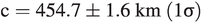 , and a volume-equivalent radius of
  . In addition, both the limb profiles and the tracking of Ceres’ main bright spot (emplaced in what is known today as Occator crater) allowed constraining the spin to
  (right ascension) and
  (declination). The shape was further used to place constraints on Ceres’ internal structure. First, it suggested that Ceres is a relaxed object in hydrostatic equilibrium. Second, using the determined density of
  along with the a and c semi-axes, Thomas et al. (Reference Thomas, Parker and McFadden2005) concluded that Ceres is most likely a differentiated object. These HST images were further used by Li et al. (Reference Li, McFadden and Parker2006) to constrain Ceres’ geometric and single-scattering albedos (respectively,
  and
and  at 535 nm) and to produce the very first spatially resolved surface albedo maps of Ceres. The maps reveal a small albedo contrast (typically
  with respect to the average for most of the surface) with the bright spot being ∼8% brighter than Ceres’ average albedo.
Carry et al. (Reference Carry2008) performed a similar analysis using Keck/NIRC2 adaptive optics J/H/K imaging observations. Whereas they also found that Ceres’ shape can be well described by that of an oblate spheroid, they derived different semi-axes values with respect to the HST results (Thomas et al., Reference Thomas, Parker and McFadden2005), namely  and
and  , and a volume-equivalent radius of
  , implying a ∼5% higher density, namely
  . Concerning the internal structure, the Carry et al. (Reference Carry2008) study agreed with the findings by Thomas et al. (Reference Thomas, Parker and McFadden2005) that Ceres must be differentiated. Note that observations by Dawn imply that Ceres’ interior is only partially differentiated (Park et al., Reference Park, Konopliv and Bills2016; Chapter 12). Finally, Carry et al. (Reference Carry2008) also constrained the spin axis to
  (right ascension) and
  (declination) and produced albedo maps in the different bands (J, H, K), revealing an albedo variegation similar to the one reported by Li et al. (Reference Li, McFadden and Parker2006).
Recently, Ceres has been imaged by the SPHERE instrument at the VLT revealing so far the most spectacular view of this object from Earth at a resolution of 4.4 km/pixel (Vernazza et al., Reference Vernazza, Jorda and Sevecek2020; Figure 1.4). A reflectance map based on the best-quality image (Vernazza et al., Reference Vernazza, Jorda and Sevecek2020) reveals a much higher albedo contrast (around ∼20%) than previously reported (Li et al., Reference Li, McFadden and Parker2006; Carry et al., Reference Carry2008).
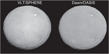
Figure 1.4 Comparison of the VLT/SPHERE deconvolved images of Ceres (left) with a synthetic projection of the Dawn 3D shape model produced with OASIS and with albedo information (right). The deconvolved image (left) shows a clear–dark–clear border, which is a deconvolution artefact.
When confronting Earth-based observations of Ceres with those of the NASA Dawn mission, it appears that the true dimensions of Ceres ( ,
,  , and
, and  , and a volume-equivalent radius of
  ; Russell et al., Reference Russell, Raymond and Ammannito2016; Park et al., Reference Park, Vaughan and Konopliv2019) as well as its density (
 ; Russell et al., Reference Russell, Raymond and Ammannito2016) fall in between those determined early on by Thomas et al. (Reference Thomas, Parker and McFadden2005) and Carry et al. (Reference Carry2008) – although closer to those of Carry et al. (see Table 1.3). In addition, Ceres’ exact pole coordinates (a right ascension of
  and a declination of
  ; Park et al., Reference Park, Vaughan and Konopliv2019) are very close to those derived earlier by Carry et al. (Reference Carry2008).
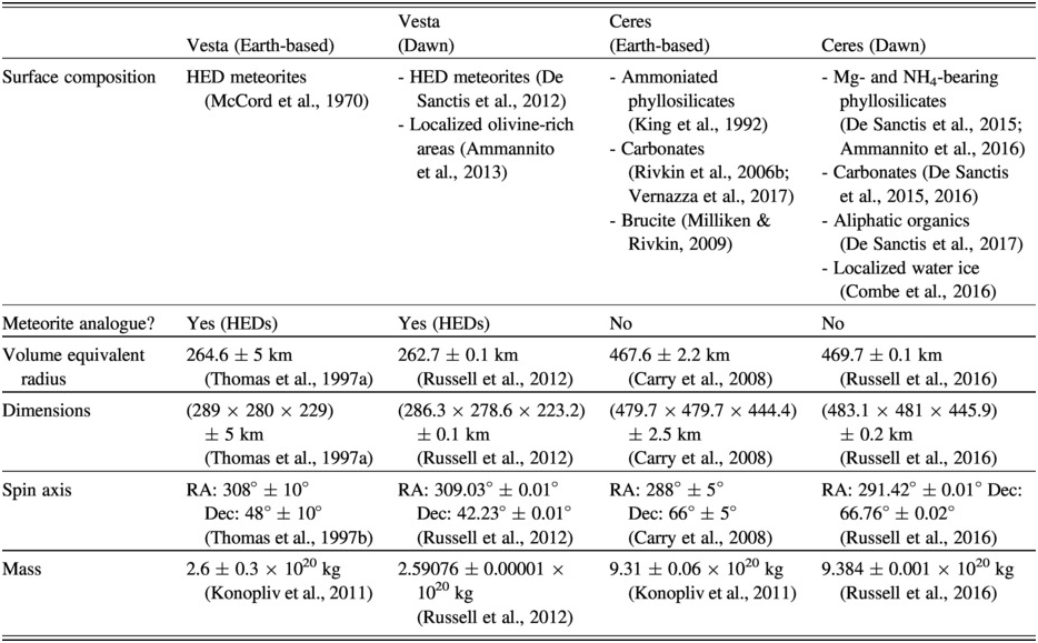
Table 1.3 Vesta and Ceres’ physical and geological properties from Dawn compared to those derived from Earth.
| Vesta (Earth-based) | Vesta (Dawn) | Ceres (Earth-based) | Ceres (Dawn) | |
|---|---|---|---|---|
| Surface composition | HED meteorites (McCord et al., Reference McCord, Adams and Johnson1970) | - HED meteorites (De Sanctis et al., Reference De Sanctis, Ammannito and Capria2012) - Localized olivine-rich areas (Ammannito et al., Reference Ammannito, DeSanctis and Ciarniello2013) | - Ammoniated phyllosilicates (King et al., Reference King, Clark, Calvin, Sherman and Brown1992) - Carbonates (Rivkin et al., Reference Rivkin, Li and Milliken2006b; Vernazza et al., Reference Vernazza, Beck, Elkins-Tanton and Weiss2017) - Brucite (Milliken & Rivkin, Reference Milliken and Rivkin2009) | - Mg- and NH4-bearing phyllosilicates (De Sanctis et al., Reference De Sanctis, Ammannito and Raponi2015; Ammannito et al., Reference Ammannito, DeSanctis and Ciarniello2016) - Carbonates (De Sanctis et al., Reference De Sanctis, Ammannito and Raponi2015, Reference De Sanctis, Raponi and Ammannito2016) - Aliphatic organics (De Sanctis et al., Reference De Sanctis, Ammannito and McSween2017) - Localized water ice (Combe et al., Reference Combe, McCord and Tosi2016) |
| Meteorite analogue? | Yes (HEDs) | Yes (HEDs) | No | No |
| Volume equivalent radius | 264.6 ± 5 km (Thomas et al., Reference Thomas, Emery and Trilling1997a) | 262.7 ± 0.1 km (Russell et al., Reference Russell, Raymond and Ammannito2012) | 467.6 ± 2.2 km (Carry et al., Reference Carry2008) | 469.7 ± 0.1 km (Russell et al., Reference Russell, Raymond and Ammannito2016) |
| Dimensions | (289 × 280 × 229) ± 5 km (Thomas et al., Reference Thomas, Emery and Trilling1997a) | (286.3 × 278.6 × 223.2) ± 0.1 km (Russell et al., Reference Russell, Raymond and Ammannito2012) | (479.7 × 479.7 × 444.4) ± 2.5 km (Carry et al., Reference Carry2008) | (483.1 × 481 × 445.9) ± 0.2 km (Russell et al., Reference Russell, Raymond and Ammannito2016) |
| Spin axis | RA: 308° ± 10° Dec: 48° ± 10° (Thomas et al., Reference Thomas, Binzel and Gaffey1997b) | RA: 309.03° ± 0.01° Dec: 42.23° ± 0.01° (Russell et al., Reference Russell, Raymond and Ammannito2012) | RA: 288° ± 5° Dec: 66° ± 5° (Carry et al., Reference Carry2008) | RA: 291.42° ± 0.01° Dec: 66.76° ± 0.02° (Russell et al., Reference Russell, Raymond and Ammannito2016) |
| Mass | 2.6 ± 0.3 × 10²⁰ kg (Konopliv et al., Reference Konopliv, Asmar and Folkner2011) | 2.59076 ± 0.00001 × 10²⁰ kg (Russell et al., Reference Russell, Raymond and Ammannito2012) | 9.31 ± 0.06 × 10²⁰ kg (Konopliv et al., 2011) | 9.384 ± 0.001 × 10²⁰ kg (Russell et al., Reference Russell, Raymond and Ammannito2016) |
While the superior spatial resolution of the Dawn images has not drastically changed our knowledge of Ceres’ dimensions and rotation axis, the same cannot be said regarding the surface topography and the variegation of the albedo across its surface. Schröder et al. (Reference Schröder, Mottola and Carsenty2017) have shown that Ceres’ brightest spot corresponds to several extremely bright yet small areas within Occator crater, whose maximum size is ∼10 km in diameter (Cerealia Facula) and whose average visual normal albedo is  , reaching locally a visual normal albedo close to unity at a scale of 35 m/pixel (see Chapter 10). The amplitude of the albedo variegation is thus much higher than that deduced from the SPHERE images considering that the average albedo is around 0.1.
Regarding the surface topography, Ceres possesses a heavily cratered surface with a paucity of large craters, suggesting that relaxation has occurred (Marchi et al., Reference Marchi, Ermakov and Raymond2016). In contrast, craters can hardly be identified (at least not unambiguously) in the VLT/SPHERE images. This may be due to the morphology of D > 30 km craters (size limit above which craters can be resolved with VLT/SPHERE) as suggested by Vernazza et al. (Reference Vernazza, Jorda and Sevecek2020). D > 30 km craters on Ceres are essentially flat floored, implying a smaller contrast between the crater floor and the crater rim than in the case of simple bowl shaped craters. Adding to that, a nonperfect correction of the atmospheric turbulence may lead to a global absence of contrast due to the topography in the deconvolved VLT/SPHERE images of Ceres. The same phenomenon is also observed in the case of other C-complex asteroids observed by VLT/SPHERE, such as (10) Hygiea (Vernazza et al., Reference Vernazza, Jorda and Sevecek2020) and (704) Interamnia (Hanus et al., Reference Hanus, Vernazza and Viikinkoski2020).
1.3.1.2 (4) Vesta
A few years after the discovery of the prominent Vesta family (Binzel & Xu, Reference Binzel, DeMeo and Turtelboom1993), HST imaging observations of Vesta revealed the presence of an impact crater ∼460 km in diameter near its south pole (Thomas et al., Reference Thomas, Emery and Trilling1997a), thus strengthening the hypothesis of a collisional origin for Vesta-like bodies. The HST images were further used to constrain Vesta’s spin, shape, and density, and to produce albedo, elevation, and compositional maps of its surface (Binzel et al., Reference Binzel, Gaffey and Thomas1997; Thomas et al., Reference Thomas, Emery and Trilling1997a, Reference Thomas, Binzel and Gaffey1997b).
Thomas et al. (Reference Thomas, Emery and Trilling1997a) found that the shape of Vesta can be well described by a triaxial ellipsoid of semi-axes  ,
,  , and
, and  , and a volume-equivalent radius of
  . By combining the volume with the best mass estimates, they derived a mean density in the
  range. In addition, the spin was constrained to
  (right ascension) and
  (declination) (Thomas et al., Reference Thomas, Binzel and Gaffey1997b). The pole solution as well as the dimensions, including the volume-equivalent diameter, are very close to those derived from the Dawn imaging data (see Russell et al., Reference Russell, Raymond and Ammannito2012 and Table 1.3).
The HST images further revealed a strong albedo variegation across the surface (Binzel et al., Reference Binzel, Gaffey and Thomas1997), as well as the presence of a prominent central peak within the impact basin whose height was estimated to be of the order of 13 km above the deepest part of the floor (Thomas et al., Reference Thomas, Emery and Trilling1997a). The Dawn mission actually revealed the existence of two overlapping basins in the south polar region and a central peak whose height rivals that of Olympus Mons on Mars (e.g., Jaumann et al., Reference Jaumann, Williams and Buczkowski2012; Marchi et al., Reference Marchi, Ermakov and Raymond2012; Russell et al., Reference Russell, Raymond and Ammannito2012; Schenk et al., Reference Schenk, O’Brien and Marchi2012). The images of the Dawn mission also allowed the production of a high-resolution map of the albedo across Vesta’s surface, revealing the second greatest variation of normal albedo of any asteroid yet observed after Ceres (the normal albedo varies between ∼0.15 and ∼0.6; Schröder et al., Reference Schröder, Mottola and Carsenty2014; see also Chapter 6).
Recently, VLT/SPHERE images have recovered the surface of Vesta with a great amount of detail (Figure 1.5; Fetick et al., Reference Fetick, Jorda and Vernazza2019). Most of the main topographic features present across Vesta’s surface can be readily recognized from the ground. This includes the south pole impact basin and its prominent central peak, several D ≥ 25 km sized craters, and also Matronalia Rupes, including its steep scarp and its small and big arcs. On the basis of these observations, it follows that next-generation telescopes with mirror sizes in the 30–40 m range (e.g., the Extremely Large Telescope, hereafter ELT) should in principle be able to resolve the remaining major topographic features of (4) Vesta (i.e., equatorial troughs, north–south crater dichotomy), provided that they operate at the diffraction limit in the visible range.

Figure 1.5 Comparison of the VLT/SPHERE deconvolved images of Vesta (left column) with synthetic projections of the Dawn 3D shape model produced with OASIS and with albedo information (right column). No albedo data is available from Dawn for latitudes above 30° N (orange line). The main structures that can be identified in both the VLT/SPHERE images and the synthetic ones are highlighted: craters are embedded in squares and albedo features in circles (from Fetick et al., Reference Fetick, Jorda and Vernazza2019).
A black and white version of this figure will appear in some formats. For the color version, refer to the plate section.
1.3.2 Overview of Earth-based Imaging Campaigns of Main Belt Asteroids
The large angular diameter of (1) Ceres and (4) Vesta at opposition (up to ∼840 mas and ∼700 mas, respectively) explains why these two bodies have been the subjects of in-depth studies using first-generation high angular resolution imaging systems such as HST (resolution of ∼50 mas). There are a few other Main Belt bodies that possess relatively large angular diameters at opposition ((2) Pallas: ∼540 mas; (324) Bamberga: ∼380 mas; (3) Juno, (7) Iris, and (10) Hygiea: ∼325 mas) and that could have been valuable targets for dedicated observing campaigns using either HST or Keck/NIRC2. This has, however, only been the case for the largest of them ((2) Pallas; Schmidt et al., Reference Schmidt, Thomas and Bauer2009; Carry et al., Reference Carry, Vachier and Berthier2010a). Overall, before the advent of the SPHERE instrument at the VLT, sparse Keck/NIRC2 imaging data had been collected for many D > 100 km asteroids. Furthermore, these data were rarely acquired when the targets were at opposition, leading to non-optimal resolution for the observations of these bodies (Hanus et al., Reference Hanus, Marsset and Vernazza2017b). Hereafter, we describe some important constraints that have been collected for D > 100 km asteroids based on high angular resolution imaging observations.
1.3.2.1 Asteroid Densities and Internal Structures
Density is the physical property that constrains best the interior of asteroids. Unfortunately, the latter has only been measured for a handful of asteroids (mostly in the case of multiple asteroids but also via in-situ space missions). Importantly, most D < 100 km asteroids are seen as collisionally evolved objects (Morbidelli et al., Reference Morbidelli, Bottke, Nesvorny and Levison2009) whose internal structure can be largely occupied by voids (called macroporosity, reaching up to 50–60% in some cases; Carry, Reference Carry2012; Scheeres et al., Reference Scheeres, Britt, Carry, Holsapple, Michel, DeMeo and Bottke2015), thus limiting our capability to interpret meaningfully their bulk density in terms of composition(s). On the contrary, large bodies (D > 100 km) are seen as primordial remnants of the early Solar System (Morbidelli et al., Reference Morbidelli, Bottke, Nesvorny and Levison2009); that is their internal structure has likely remained intact since their formation (they can be seen as the smallest protoplanets). For most of these objects, the macroporosity is likely minimal (<20%) and their bulk density is therefore an excellent tracer of their bulk composition.
Following the discovery by the Galileo spacecraft of the first Main Belt asteroid’s satellite (Dactyl, around (243) Ida; Chapman et al., Reference Chapman, Veverka and Thomas1995; Belton et al., Reference Belton, Chapman and Thomas1995), high angular resolution imaging observations of the largest Main Belt asteroids were performed during the subsequent ∼15 years to search for the presence of moons/companions. Note that accurate 3D shape reconstruction algorithms based on AO data such as KOALA (Carry et al., Reference Carry, Dumas and Kaasalainen2010b) and ADAM (Viikinkoski et al., Reference Viikinkoski, Kaasalainen and Durech2015a) were not available during that time frame, leaving the moon search and the subsequent characterization of its orbit as the most compelling science objective. Indeed, direct imaging observations of multiple-asteroid systems are the most efficient approach from Earth for deriving precise asteroid masses. Specifically, the images provide constraints on the orbital parameters of the moon(s) and hence the total mass of the system. In the case of (a) small companion(s), the total mass is dominated by the primary implying that the mass of the primary can be well constrained (usually with a <10% uncertainty). The only other way to constrain masses of large asteroids with similar precision is via dedicated interplanetary missions, either a fly-by for the largest ones (as in the case of (21) Lutetia) or a rendezvous (e.g. Dawn mission, OSIRIS-REx, Hayabusa 1 & 2). Note that the orbital properties of the moon(s) can be used to constrain the dynamical quadrupole J2; by comparing the latter with the J2 derived from the 3D shape of the primary, one can search for the presence or absence of a mass concentration within the primary, hence a differentiated internal structure (e.g., Pajuelo et al., Reference Pajuelo, Carry and Vachier2018).
At the time of writing the Asteroid III book, seven multiple systems were known among the largest (D > 90 km) Main Belt asteroids (Merline et al., Reference Merline, Weidenshilling, Durda, Bottke, Cellino, Paolicchi and Binzel2002), and this number increased by a factor of two at the time of writing the Asteroid IV book (Margot et al., Reference Margot, Pravec, Taylor, Michel, DeMeo and Bottke2015). Since then, only one multiple system has been discovered among large Main Belt asteroids ((31) Euphrosyne and its moon; see Vernazza et al., Reference Vernazza, Carry and Vachier2019). Among these 15 multiple systems, six are triple systems, the first to be discovered being the one of (87) Sylvia (Marchis et al., Reference Marchis, Descamps, Hestroffer and Berthier2005). Two thirds of these multiple systems belong to the C-complex, while the remaining systems belong either to the P or M classes. Surprisingly, there are currently no large S-types with known companions. Whereas the observed S/C type dichotomy may be interpreted as a consequence of compositional differences (hence different material strengths) implying a different response to impacts between the water-poor silicate-rich S-types and the water-rich C-types, the existence of the metal/silicate-rich Kalliope and Kleopatra systems complicates the picture.
Hereafter, we summarize current knowledge regarding the bulk composition of the main taxonomic classes (Figure 1.6). In the case of the largest S-type asteroids, the derived densities are consistent with those of ordinary chondrites (Viikinkoski et al., Reference Viikinkoski, Kaasalainen and Durech2015b; Hanus et al., Reference Hanus, Viikinkoski and Marchis2017b, Reference Hardersen, Cloutis and Reddy2019; Marsset et al., Reference Masiero, Grav and Mainzer2017), implying – contrary to asteroid (4) Vesta – an absence of large-scale differentiation for these bodies, which is in agreement with the thermal history of ordinary chondrites (Huss et al., Reference Huss, Rubin, Grossman, Lauretta and McSween2006; Monnereau et al., Reference Monnereau, Toplis, Baratoux and Guignard2013). Similarly, the density of the largest CM-like bodies (Cg/Cgh types) is consistent with that of CM chondrites, suggesting a homogeneous internal structure for these bodies (Carry et al., Reference Carry, Vachier and Berthier2019). Concerning the remaining large (D > 200 km) C-complex bodies (C, Cb, Cg, and most B-types apart from Pallas), their density is in the 1.4–2.0 g/cm3 range (Marchis et al., Reference Marchi, Ermakov and Raymond2012; Hanus et al., Reference Hanus, Vernazza and Viikinkoski2020; Vernazza et al., Reference Vernazza, Jorda and Sevecek2020), implying a high water fraction for these bodies. Modeling results by Beauvalet and Marchis (Reference Beauvalet and Marchis2014) in the case of (45) Eugenia further suggest the presence of a denser core, possibly consistent with an early differentiation. A differentiated interior has also been advocated in the case of the largest C-type, (1) Ceres (e.g., Thomas et al., Reference Thomas, Parker and McFadden2005; Park et al., Reference Park, Konopliv and Bills2016; Chapter 12). It is too early to conclude that all large water-rich C-types underwent differentiation, yet thermal evolution models suggest that such a trend was quasi unavoidable for D > 200 km objects consisting initially of a 70% rock, 30% ice composition by mass (Neveu & Vernazza, Reference Neveu and Vernazza2019). Finally, large P-type asteroids for which precise density estimates are available indicate a density in the 1.0–1.3 g/cm3 range that appears substantially lower than that of water-rich C-types. It is worth mentioning that, for the two largest bodies – (87) Sylvia and (107) Camilla – the presence of a small dense core is predicted (Pajuelo et al., Reference Pajuelo, Carry and Vachier2018, Carry et al., Reference Carry, Vernazza and Vachier2021). It is presently unclear whether these bodies are more water-rich than C-types or if they formed with substantial porosity (70–75%), as observed in the case of comet 67P/Churyumov-Gerasimenko (Jorda et al., Reference Jorda, Gaskell and Capanna2016).

Figure 1.6 Density of some of the largest asteroids. Asteroids are grouped following their spectral classification. The relative sizes of the dots follow the relative diameters of the bodies in logarithmic scale. Error bars are 1-sigma. The science based on these density estimates can be retrieved in Paetzold et al. 2011, Russell et al. 2012, 2016, Viikinkoski et al. 2015b, Marsset et al. 2017, Hanus et al. 2017a, b, Pajuelo et al. 2018, Carry et al. 2019a, b, Ferrais et al. 2020, Hanus et al. 2020, Marsset et al. 2020, Vernazza et al. 2020, Vernazza et al. 2021, Yang et al. 2020 and Dudzinski et al. 2020.
A black and white version of this figure will appear in some formats. For the color version, refer to the plate section.
1.3.2.2 Asteroid Shapes
Because of their large masses, Solar System bodies with diameters larger than ∼900 km possess rounded, ellipsoidal shapes, consistent with hydrostatic equilibrium, which is a part of the current IAU definition of a planet or a dwarf planet. On the other side of the mass range, very small bodies (diameters < 100 km) tend to possess highly irregular shapes, with the notable exception of some D < 5 km bodies that are affected by the so-called YORP effect (Yarkovsky–O’Keefe–Radzievskii–Paddack; Rubincam, Reference Rubincam2000; Vokrouhlický et al., Reference Vokrouhlický, Nesvorný and Bottke2003), and which have similar shapes to a spinning top (e.g., Ryugu, or Bennu; Nolan et al., Reference Nolan, Magri and Howell2013; Watanabe et al., Reference Watanabe, HiraBayashi and Hirata2019). However, it remains to be tested at what size range the shape of a typical minor body transits from a nearly rounded equilibrium shape to an irregular shape and to what extent this size range depends on factors such as the bulk composition of the minor planet or its collisional and thermal history (Hanus et al., Reference Hanus, Vernazza and Viikinkoski2020).
Recently, an imaging survey of a substantial fraction of all D > 100 km Main Belt asteroids (sampling the main compositional classes) has been conducted using VLT/SPHERE (Vernazza et al., Reference Vernazza, Broz and Drouard2018, Reference Vernazza, Jorda and Sevecek2020; Viikinkoski et al., Reference Viikinkoski, Vernazza and Hanus2018; Carry et al., Reference Carry, Vachier and Berthier2019; Fetick et al., Reference Fetick, Jorda and Vernazza2019; Hanus et al., Reference Hardersen, Cloutis and Reddy2019, Reference Hanus, Vernazza and Viikinkoski2020; Ferrais et al., Reference Ferrais, Vernazza and Jorda2020; Marsset et al., Reference Marsset, Broz and Vernazza2020; Yang et al., Reference Yang, Hanus and Carry2020; Figure 1.7). So far, it appears that water-rich asteroids with D > 250 km have shapes close to equilibrium (Ferrais et al., Reference Ferrais, Vernazza and Jorda2020; Yang et al., Reference Yang, Hanus and Carry2020). At similar sizes, rocky bodies such as (3) Juno appear more irregular. Still, rocky or even metal-rich bodies such as Psyche with D > 200 km have shapes that are closer to that of an ellipsoid than D < 200 km bodies (Ferrais et al., Reference Ferrais, Vernazza and Jorda2020), suggesting that the transition from a regular equilibrium shape to a fully irregular shape is smooth. The equilibrium shapes of water-rich bodies suggest that these bodies were fluid during their history, either as the result of early thermal heating leading to aqueous alteration of their interiors or because of large impacts and subsequent reaccumulation (e.g., Vernazza et al., Reference Vernazza, Jorda and Sevecek2020; Yang et al., Reference Yang, Hanus and Carry2020).

Figure 1.7 VLT/SPHERE images deconvolved with the MISTRAL algorithm (Fusco et al., Reference Fusco, Mugnier, Conan, Wizinowich and Bonaccini2003) of a sample of D > 200 km asteroids. The relative sizes are respected, and the scale is indicated on the plot. The objects appear according to decreasing values of their volume equivalent diameter (see Table 1.1). The science based on these images can be retrieved from Fetick et al. (Reference Fetick, Jorda and Vernazza2019), Hanus et al. (Reference Hardersen, Cloutis and Reddy2019, Reference Hanus, Marsset and Vernazza2020), Ferrais et al. (Reference Ferrais, Vernazza and Jorda2020), Marsset et al. (Reference Marsset, Broz and Vernazza2020), Vernazza et al. (Reference Vernazza, Jorda and Sevecek2020), Yang et al. (Reference Yang, Hanus and Carry2020) and Carry et al. (Reference Carry, Vernazza and Vachier2021).
1.3.2.3 Cratering History of D > 100 km Asteroids
Prior to the first light of the adaptive-optics SPHERE imaging system at ESO/VLT in 2014, the characterization of the surface topography of asteroids had only been performed via dedicated in situ space missions (Galileo, NEAR Shoemaker, Hayabusa 1&2, Rosetta, Dawn, OSIRIS-REx) with the notable exception of Vesta’s south pole impact basin detected by HST (Thomas et al., Reference Thomas, Binzel and Gaffey1997a). The SPHERE survey of D > 100 km asteroids (Vernazza et al., Reference Vernazza, Broz and Drouard2018) has drastically augmented the number of asteroid craters detected from Earth. For example, Fetick et al. (Reference Fetick, Jorda and Vernazza2019) detected nine craters larger than 25 km in diameter on Vesta (e.g., Figure 1.5), Hanus et al. (Reference Hardersen, Cloutis and Reddy2019) identified eight impact craters 20–40 km in diameter on (7) Iris, while Marsset et al. (Reference Marsset, Broz and Vernazza2020) identified 36 craters larger than 30 km in diameter on (2) Pallas. The large number of D > 30 km craters on Pallas appears to be consistent with its high inclination (∼35°) implying a more violent collisional history than that of Vesta or Ceres. Also, VLT/SPHERE observations of asteroid (89) Julia (Vernazza et al., Reference Vernazza, Broz and Drouard2018), a D ∼ 140 km S-type asteroid and the parent body of a small collisional family that consists of 66 known members with D < 2.5 km, have revealed the presence of an impact crater (∼75 km wide) that could be the origin of this family. These results highlight the fact that the geological history of asteroids can now be investigated from the ground for a large number of asteroids, thus nicely complementing higher resolution data obtained in situ for a few bodies.
1.4 Conclusion and Perspective
When confronting the measurements of the global physical properties (average surface composition, size, shape, spin, rotation period, density) obtained from Earth with those obtained in-situ for both Vesta and Ceres, it appears that the results are about the same within errors (Table 1.3). This underlines the reliability of Earth-based observations and of the methods employed to analyze the data, especially when they are collected from the ground requiring atmospheric correction. Notably, recent VLT/SPHERE imaging observations have demonstrated in a striking manner how the gap between interplanetary missions and ground-based observations is getting narrower (Fetick et al., Reference Fetick, Jorda and Vernazza2019; Vernazza et al., Reference Vernazza, Jorda and Sevecek2020). With the advent of extremely large telescopes (ELT, GMT, TMT), the science objectives of future interplanetary missions to Main Belt asteroids will have to be carefully thought out so that these missions will complement – not duplicate – what will be achieved via Earth-based telescopic observations. For instance, future ELT adaptive-optics imaging of main-belt asteroids will allow us to resolve craters down to ∼5 km in size, implying that we shall be able to characterize their global geological history from the ground. This implies that geological and geomorphological studies (based on high angular resolution imaging data) might become – during the coming decade – the prime science objectives that will be conducted from Earth in the case of large D > 100 km asteroids, dethroning studies related to the nature/origin of these bodies (deduced from the analysis of their spectra). Interplanetary missions to Main Belt asteroids performing cosmochemistry experiments, landing, and eventually a sample return should be preferred at the forefront of in-situ exploration as these would ideally complement the investigations conducted from Earth. In particular, IDP-like asteroids as well as the rare L-, Xe-, Xn- and O-types should be preferred targets as little is known regarding these bodies due to the paucity/absence of samples for these objects in our collections.