


Introduction
In developing countries, conventional solutions to market failures, including physical collateral, are a barrier to access credit for most small-scale farmers. However, access to financial services by small-scale farmers has been considered as a way to improve smallholder farm productivity (Carter and Olinto Reference Carter and Olinto2003; Foltz Reference Foltz2004). In the short run, credit can help farmers increase their purchasing power to acquire necessary production inputs and finance their operating expenses, while, in the long run, it can improve farmers’ ability to make profitable investments (Conning and Udry Reference Conning, Udry, Evenson and Pingali2007). Unfortunately, most farmers are small-scale and rely almost exclusively on their equity capital to purchase inputs.
Financial system provides liquidity to poor farmers to buy inputs such as seeds, fertilizers, and agrochemicals, which increase agricultural productivity. However, the existence of credit market imperfections, particularly those arising from asymmetric information, can cause a misallocation of resources and a suboptimal use of inputs in farm production (Stiglitz and Weiss Reference Stiglitz and Weiss1981). This misallocation can in turn negatively affect farm productivity and result in lower income for constrained farmers compared to unconstrained farmers (Petrick Reference Petrick2004; Ali, Deininger and Duponchel Reference Ali, Deininger and Duponchel2014).
Financial constraints affect farm productivity through their adverse effects on smallholders’ farm output and investment (Guirkinger and Boucher Reference Guirkinger and Boucher2008; Barrett et al. Reference Barrett, Bellemare and Hou2010; Karlan et al. Reference Karlan, Osei, Akoto and Udry2014). As most smallholder farmers tend to be poor, equity capital financing of necessary agricultural inputs is very difficult. Credit can help farmers purchase the inputs required to ensure increased agricultural output. In China, by removing credit constraints, agricultural productivity and rural household income could be increased by approximately 23.3% (Dong, Lu, and Featherstone Reference Dong, Lu and Featherstone2012). Based on farm data from Russia, Kumbhakar and Bokusheva (Reference Kumbhakar and Bokusheva2009) show that expenditure constraints caused, on average, a potential output loss of 20%.
In East Africa, a majority of smallholder farmers rely on savings from their low income for investments, which limits their expansion (Salami et al. Reference Salami, Kamara and Brixiova2010). In Peru, productivity is lowered by credit constraints (Guirkinger and Boucher Reference Guirkinger and Boucher2008). In Ghana, Akudugu (Reference Akudugu2016) finds that both formal and informal credit have positive and significant effects on agricultural productivity. However, formal credit has lower effects on agricultural productivity than informal credit does. In Rwanda, the elimination of all credit constraints in rural areas could increase output by approximately 17% (Ali, Deininger, and Duponchel Reference Ali, Deininger and Duponchel2014).
Despite its importance, the impact of financial constraints on smallholder farm productivity has been poorly measured and often not properly identified in previous studies. Empirical literature on the impact of credit constraints on input allocation decisions and farm productivity remains limited in developing countries. In the presence of financial constraints, neither cost minimization nor profit maximization behaviors are valid for modeling producers’ input use decisions. To accommodate this problem, output maximization subject to a specified expenditure on variable inputs is often used as rational economic behavior. This calls for the use of an alternative dual approach, the indirect production function approach (Shephard Reference Shephard1974).
In Burkina Faso, the low liquidity of farms and limited access to external finance due to financial market imperfections seriously limits producers’ space for input allocation decisions. Data from the Ministry of Agriculture and Hydro-Agricultural Development indicate that only 20% of smallholder farmers had access to agricultural credit in 2018. In this context, modern inputs are used very little, and most of the agricultural growth is due to the expansion of the area under cultivation (Auger Reference Auger2018).
Hence, a limited budget for the purchase of variable inputs may induce nonoptimal input usage, which in turn results in productivity losses. Faced with expenditure constraints, public policy makers in Burkina Faso have set up an input subsidy program for smallholder farms of strategic cereal crops such as maize. Maize is the leading cereal crop in Burkina Faso with about 20% of the area planted, 40% of cereal production and is the main staple food for most householdsFootnote 1 .
Maize production faces multiple constraints such as the low yields estimated at 1,753 kg per hectare, the high dependence on rainfall, and the poor access to financial resources for producers due to low savings and difficulties in accessing credit. Agricultural statistics reveal that in 2020, the proportion of producers using modern inputs is around 20% for improved seeds, 68% for NPK, and 52% for urea. Only 15% of maize producers combine all three types of modern inputsFootnote 2 .
Improving maize productivity remains one of the priorities of agricultural policy and poverty reduction in Burkina Faso. Due to financial constraints, smallholder maize producers do not have sufficient financial resources to acquire chemical fertilizers and improved seeds. This situation has an impact on the allocation of factors and the productivity of maize producers in Burkina Faso. However, there has been no rigorous research work to assess the impact of budget constraints on the factor allocation and productivity of smallholder maize producers in Burkina Faso to better identify the most appropriate agricultural policy.
This paper tests the hypothesis that the liquidity constraint for the purchase of variable inputs leads to a suboptimal allocation of inputs and a decline in the productivity of small-scale maize producers in Burkina Faso. The rest of the paper is organized as follows. In Section 2, we present the modeling farms’ production decisions under expenditure constraints. The method of data collection and descriptive statistical analysis are presented in Section 3. Section 4 discusses the results, and Section 5 shows the conclusions and policy implications.
Modeling farms’ production decisions under expenditure constraints
In this section, we develop a basic theoretical model that links farmers’ optimization behavior under expenditure constraints. The indirect production function (IPF) is an appropriate tool to use when the objective is to maximize output subject to a given technology, a set of quasi-fixed inputs, and a given budget for the purchase of variable inputs (Kumbhakar and Bokusheva Reference Kumbhakar and Bokusheva2009).
The indirect production function
In their factor allocation decisions, smallholder maize farmers in Burkina Faso face financial constraints. This calls for the use of the indirect production function to model their behavior. The producer’s objective is to maximize output, subject to the budget constraint. The problem can be written as,
 $$Max\,\,\,y = f\left( {x,z} \right)$$
 $${\rm subject \ to}\;C = \omega 'x$$
where y is the output, x denotes a vector of N variable inputs, z denotes the quasi-fixed input vector of order J, C represents the budget available for the purchase of variable inputs, $\omega $
denotes the vector of variable input prices, and
$\omega $
denotes the vector of variable input prices, and $f\left( {x,z} \right)$
is a nondecreasing, twice continuously differentiable and quasi-concave function of
$f\left( {x,z} \right)$
is a nondecreasing, twice continuously differentiable and quasi-concave function of ${\rm{\;}}x$
and z.
${\rm{\;}}x$
and z.
The Lagrangian for this problem can be written as,
 $$L = f\left(. \right) + \lambda \left( {C - \omega 'x} \right)$$
where $\lambda $
denotes the Lagrange multiplier.
$\lambda $
denotes the Lagrange multiplier.
Solving the first-order conditions for the problem ${f_j} = \lambda {\omega _j}$
,
${f_j} = \lambda {\omega _j}$
, $\forall \;j$
and
$\forall \;j$
and $C = \omega 'x$
, we obtain the solution of the endogenous variables in terms of the exogenous variables, that is,
$C = \omega 'x$
, we obtain the solution of the endogenous variables in terms of the exogenous variables, that is,
 $${x_j} = {g_j}\left( {\omega ,C,z} \right),\;\;\forall \;j = 1, \ldots ,N$$
 $$\lambda = {g_j}\left( {\omega ,C,z} \right)$$
(4) represents the input demand function; according to economic theory, the demand function must be homogeneous of degree zero in input prices and expenditure, exhaustive, and symmetrical.
(5) represents the marginal productivity of the expenditure.
Substituting ${x_j} = {g_j}\left( {\omega ,C,z} \right)$
from equation (4) into equation (1) of the production function, we obtain the indirect production function (IPF) as
${x_j} = {g_j}\left( {\omega ,C,z} \right)$
from equation (4) into equation (1) of the production function, we obtain the indirect production function (IPF) as
 $$y = \varphi \left( {\omega ,C,z} \right)$$
where $\varphi \left(. \right)$
represents the indirect production function.
$\varphi \left(. \right)$
represents the indirect production function.
The IPF expresses the maximum attainable output given the availability of funds, the price of variable inputs, and the amounts of quasi-fixed inputs. In addition to the usual symmetry restrictions on the coefficients, economic theory states that the IPF is homogeneous of degree zero in input prices and expenditure. The input demand function for the input variables can be derived from the IPF by using Roy’s identity (Chambers Reference Chambers1982):
 $${x_j}\left( {\omega ,C,z} \right) = \left( {\partial y/\partial {\omega _j}} \right)/\left( {\partial y/\partial C} \right),\;j = 1, \ldots ,J$$
The marginal productivity of the expenditure can be obtained from the partial derivative of the IPF with respect to the expenditure:
 $$\lambda = \partial y/\partial C$$
If the farm has no expenditure constraints, the value of $\lambda $
will be unity, given that the maize output is measured in value terms. That is, if the farm faces an expenditure constraint, the value of
$\lambda $
will be unity, given that the maize output is measured in value terms. That is, if the farm faces an expenditure constraint, the value of $\lambda $
will exceed unity. We can also test the hypothesis that a particular farm is expenditure constrained. That is, the null hypothesis of interest is
$\lambda $
will exceed unity. We can also test the hypothesis that a particular farm is expenditure constrained. That is, the null hypothesis of interest is ${H_0}:\lambda = 1$
, which can be tested against the alternative hypothesis
${H_0}:\lambda = 1$
, which can be tested against the alternative hypothesis ${H_a}:\lambda \gt 1$
.
${H_a}:\lambda \gt 1$
.
The full econometric specification of the model of the indirect production and input demand functions is presented in the following section.
Econometric specification of the indirect production and input demand functions
The econometric model consists of the IPF and an inputs linear-approximate almost ideal demand system (AIDS). A quadratic functional translog form is chosen for the IPF to impose minimal a priori restrictions on the underlying production technology. This gives
 $$\eqalign{ln{y_i} = {\alpha _0} + \mathop \sum \limits_{j \,= 1}^J {\alpha _j}ln{\omega _{ji}} + \mathop \sum \limits_{m \,= \,1}^M {\alpha _m}ln{z_{mi}} + {\alpha _c}ln{C_i} \cr + {1 \over 2}\left\{ {\mathop \sum \limits_{k \,= \,1}^J \mathop \sum \limits_{j \,= 1}^J {\alpha _{jk}}ln{\omega _{ji}}ln{\omega _{ki}} + {\alpha _{cc}}{{\left( {ln{C_i}} \right)}^2} + \mathop \sum \limits_{L = \,1}^M \mathop \sum \limits_{m \,= \,1}^M {\alpha _{ml}}ln{z_{mi}}ln{z_i}} \right\} \cr + \mathop \sum \limits_{m \,= \,1}^M \mathop \sum \limits_{j \,= 1}^J {\alpha _{jm}}ln{w_{ji}}ln{z_{mi}} + \mathop \sum \limits_{j = 1}^J {\alpha _{jc}}ln{\omega _{ji}}ln{C_i} \cr + \mathop \sum \limits_{m \,= \,1}^F {\alpha _{mc}}ln{z_{mi}}ln{C_i} + {v_i}\;,\;i = 1, \ldots ,I}$$
Economic theory tells us that the IPF is homogeneous of degree zero in input prices and expenditure. This gives rise to the following set of restrictions on the parameters of the model:
 $$\mathop \sum \limits_{j \,= 1}^J {\alpha _j} + {\alpha _c} = 0\;\;;\;\;\;\;\;\;\;\;\;\mathop \sum \limits_{j = 1}^J {\alpha _{jk}} + {\alpha _{jc}} = 0,\;\;\;\forall j = 1,\; \ldots ,J\;;$$
 $$\mathop \sum \limits_{j \,= 1}^J {\alpha _{jm}} + {\alpha _{mc}} = 0,\;\;\forall m = 1,\; \ldots ,M\;\;;\;\;\;\;\;\;\;\;\mathop \sum \limits_{j = 1}^J {\alpha _{jc}} + {\alpha _{cc}} = 0$$
The input linear-approximate AIDS is derived in budget share form as:
 $${W_i} = {\alpha _i} + \sum\limits_j {{\gamma _{ij}}} ln{\omega _j} + {\beta _i}ln\left( {{C \over \omega }} \right) + \sum\limits_k {{\delta _{ik}}} ln{Z_k}\;,\;i = 1, \ldots .,I$$
where ${W_i}$
is the budget share of input i, and
${W_i}$
is the budget share of input i, and $\omega $
, a Stone geometric price index suggested by Deaton and Muellbauer (Reference Deaton and Muellbauer1980), is defined as:
$\omega $
, a Stone geometric price index suggested by Deaton and Muellbauer (Reference Deaton and Muellbauer1980), is defined as:
 $$ln\left( \omega \right) = \mathop \sum \limits_j {W_j}ln{\omega _j}$$
Economic theory indicates that the demand function must be homogeneous of degree zero in input prices and expenditure, exhaustive, and symmetrical. This gives rise to the following set of restrictions on the parameters:
-
i. exhaustive ( $\mathop \sum \nolimits_{\bf{i}} \boldsymbol{\alpha _i} = 1$
;
$\mathop \sum \nolimits_{\bf{i}} \boldsymbol{\beta _i} = {\bf0}$
;
$\mathop \sum \nolimits_{\bf{i}} \boldsymbol{\gamma _{ij}} = {\bf0};$
);
$\mathop \sum \nolimits_{\bf{i}} \boldsymbol{\alpha _i} = 1$
;
$\mathop \sum \nolimits_{\bf{i}} \boldsymbol{\beta _i} = {\bf0}$
;
$\mathop \sum \nolimits_{\bf{i}} \boldsymbol{\gamma _{ij}} = {\bf0};$
); -
ii. homogeneous (
$\mathop \sum \nolimits_j {\gamma _{ij}} = 0$
); -
iii. symmetrical (
${\gamma _{ij}} = {\gamma _{ji}}$
).


The AIDS model has the advantage of automatically incorporating all these properties into the estimation. The price and income elasticities can be derived from the parameter estimates as: ${\varepsilon _{ii}} = - 1 + \displaystyle{{{\gamma _{ij}}} \over {{\omega _i}}} - {\beta _i},$
own price elasticity
${\varepsilon _{ii}} = - 1 + \displaystyle{{{\gamma _{ij}}} \over {{\omega _i}}} - {\beta _i},$
own price elasticity ${\varepsilon _{ij}} = \displaystyle{{{\gamma _{ij}}} \over {{\omega _i}}} - {{{\beta _i}} \over {{\omega _i}}}{\omega _j},$
cross-price elasticity
${\varepsilon _{ij}} = \displaystyle{{{\gamma _{ij}}} \over {{\omega _i}}} - {{{\beta _i}} \over {{\omega _i}}}{\omega _j},$
cross-price elasticity ${\varepsilon _{ir}} = 1 + \displaystyle{{{\beta _i}} \over {{\omega _i}}},$
income elasticity
${\varepsilon _{ir}} = 1 + \displaystyle{{{\beta _i}} \over {{\omega _i}}},$
income elasticity
Our interest is to jointly estimate the IPF and the linear-approximate AIDS as a system of equations with the abovementioned restrictions on the parameter estimates by using the seemingly unrelated regressions (SUR) method. To this end, the demand for the other inputs of production was not considered to avoid a problem of multicollinearity. The use of input budget shares as an explained variable has the advantage of reducing the risks of heteroskedasticity (Deaton Reference Deaton1986). To estimate the model proposed, we employ data obtained from household surveys from rural areas in Burkina Faso.
Data sources and descriptive statistics
This section presents the source and the method of data collection and gives a descriptive analysis of farms’ characteristic data.
Method of data collection
The data used were collected in 2017 from 2,000 rural households as part of the evaluation of the National Land Management Program. The survey is nationally representative and covers all households residing in rural areas. The sample was drawn using a three-stage random sampling process. In the first stage, 90 communes were drawn from all 302 rural communes. In the second stage, 270 villages were chosen from the selected rural communes. In the third stage, 2,160 households were selected from the 270 villages. The data collected cover all the sociodemographic and economic characteristics and the institutional framework of rural households and their farms. After excluding rural households that do not produce maize, a sample of 969 observations was retained for the estimation of the model.
Descriptive analysis of data
Maize production depends on the level of quasi-fixed inputs, price of variable inputs, and input expenditures. Maize production is measured as the maize revenue of harvest, expressed in CFA francs using the farm-gate price. The maize quasi-fixed inputs include family labor and farmland. Family labor is estimated as the amount of labor measured in person-days that family members spent working on the maize farm. Farmland is the maize cultivated land in hectares for a growing season. A positive effect of fixed inputs on maize revenue is expected.
The main variable inputs include seed, fertilizer, and manure. The price of seed is measured by the price per kilogram of seed at the beginning of the rainy season. The price of fertilizer is captured by the average weighted price of a kilogram of NPK and urea. The price of manure is approximated by the average price of a cartload of manure. It is expected that the price of the inputs will have a positive effect on maize revenue. The maize input expenditure accounts for the overall operational costs incurred by the maize production process.
Table 1 presents the average values of the main variables used in the econometric estimates. The data indicate that in maize production, a farm household commits 1.4 hectares of land and spends approximately 90,450 CFA francs in variable inputs to achieve a revenue of 222,780 CFA francs at the end of the rainy season.
Average values for inputs involved in maize production
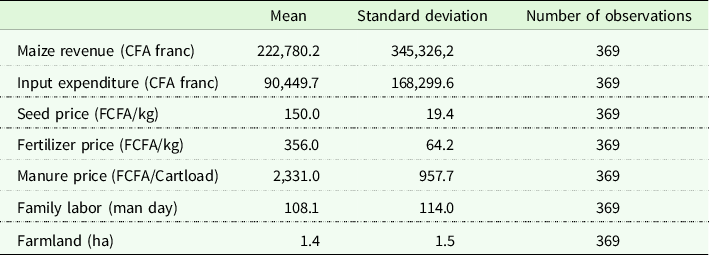
Source: Authors’ estimates from survey data.
Impact of financial constraints on maize productivity of smallholder farmers
The results from simultaneous estimations of the IPF and input demand system are reported in Table 2. The chi-squared statistics indicate that the model is well specified as a whole at the 1% level of significance. Individual tests show that most coefficients were significant at all reasonable levels.
Model parameter estimates

Source: Authors’ estimates from survey data.
*** significant at the 1% level, ** significant at the 5% level, * significant at the 10% level.
Table 3 shows that the null hypothesis of unconstrained expenditure is rejected at the 1% level of significance. The estimate for the lambda parameter (λ) is more than 1 at the 1% level of significance. Therefore, expenditure-constrained output maximization does not seem inconsistent with the current data set, suggesting that maize production faces expenditure constraints. This result was consistent with the findings of Kumbhakar and Bokusheva (Reference Kumbhakar and Bokusheva2009) for agricultural enterprises from three Russian regionsFootnote 3 , which showed that the majority of the farms studied were expenditure-constrained.
Expenditure constraint hypothesis test
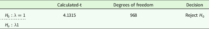
Source: Authors’ estimates from survey data.
Table 4 reports input demand elasticities for the farms considered in this analysis. The own price elasticity for fertilizer is negative and shows that a 1% increase in fertilizer price leads to a strong decrease in maize fertilizer demand of approximately 1.068%. Likewise, the own price elasticity with respect to manure price is negative, but maize manure demand decreases more weakly, by approximately 0.587% when manure price increases by 1%. However, a 1% increase in the seed price leads to a strong increase of 3.344% in maize seed demand. This surprising result can be explained by the fact that smallholder farmers are producer consumers of maize. The increase in seed prices leads to a decrease in demand for seed due to the substitution effect and the decrease in purchasing power. However, the increase in maize supply induced in the market may have a greater effect on maize income.
Input demand elasticities
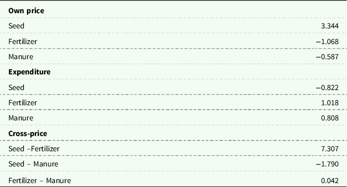
Source: Authors’ estimates from survey data.
The demand elasticities for fertilizer and manure with respect to expenditure are both positive, indicating that they are normal inputs. A 1% increase in variable input expenditure leads to a increase in fertilizer demand of approximately 1.018% and a increase in manure demand of approximately 0.808%. These results indicate that fertilizer is a superior input and manure is a necessary input. However, the demand elasticity for seeds with respect to expenditure is negative, indicating that seed is an inferior input. A 1% increase in variable input expenditure leads to a weak decrease in seed demand of approximately 0.822%. This result is explained by the fact that most farms use traditional seeds.
These results suggest that relaxing financial constraints would lead to greater fertilizer and manure usage and less seed usage. It appears that the presence of a binding liquidity constraint has led to an underutilization of fertilizer and manure and an overutilization of seed. Relaxing the expenditure constraint, therefore, would likely result in an increase in fertilizer and manure productivity.
The cross-price demand elasticities show that seed and manure inputs are complementary, while fertilizer is a substitute for seed and manure. A 1% increase in the price of fertilizer leads to a strong increase in the demand for seeds, 7.307%. Similarly, a 1% increase in the price of manure leads to a small increase in fertilizer demand, 0.042%, while seed demand falls sharply, by 1.790%.
Table 5 illustrates maize supply elasticities and the estimate of lambda (λ) for the farms considered in this analysis. The results show that maize revenue is more sensitive to changes in variable input prices compared with changes in expenditure and quasi-fixed inputs. The partial elasticity for farmland is positive and indicates that 1% increase in acreage leads to increase in maize revenue by approximately 0.077%. This result is consistent with the findings obtained by Kumbhakar and Bokusheva (Reference Kumbhakar and Bokusheva2009), which showed that the partial elasticities for land are positive (0.30) for agricultural enterprises from three Russian regions.
Maize supply elasticities
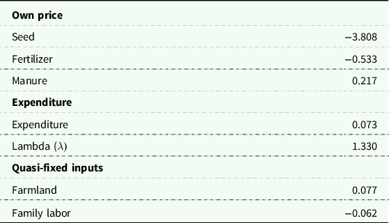
Source: Authors’ estimates from survey data.
However, the partial elasticity for family labor is negative and implies that 1% increase in family labor leads to decrease in maize income by 0.062%. This surprising result can be explained by the fact that the collective production of maize in rural areas is mostly intended for household consumption, while individual production is more often intended for the market.
The output supply elasticity with respect to the farm budget for variable inputs shows that maize revenue is expected to rise only by 0.073% for 1% increase in budget. The lambda ( $\lambda $
) value is 1.330, which confirms that the maize farms are under expenditure constraints. An expenditure of 1 CFA franc on variable inputs generates 1.330 CFA francs as maize income. This implies that a relaxation of the budget constraint leads to an increase in maize revenue by approximately 0.330 CFA franc for each 1 additional CFA franc spent on inputs, an additional gain of 25%.
$\lambda $
) value is 1.330, which confirms that the maize farms are under expenditure constraints. An expenditure of 1 CFA franc on variable inputs generates 1.330 CFA francs as maize income. This implies that a relaxation of the budget constraint leads to an increase in maize revenue by approximately 0.330 CFA franc for each 1 additional CFA franc spent on inputs, an additional gain of 25%.
These results are consistent with those reported in other developing countries, which showed that expenditure constraints caused agricultural productivity losses in Peru of 26% (Guirkinger and Boucher Reference Guirkinger and Boucher2008), in China of 23.3% (Dong, Lu, and Featherstone Reference Dong, Lu and Featherstone2012), in Russia of 20% (Kumbhakar and Bokusheva Reference Kumbhakar and Bokusheva2009), and in Rwanda of 17% (Ali, Deininger, and Duponchel Reference Ali, Deininger and Duponchel2014).
The output supply elasticity with respect to seed price is negative and shows that 1% increase in seed price leads to a strong decrease in maize revenue by approximately 3.808%. Likewise, the partial elasticity with respect to fertilizer price is negative, but maize revenue decreases more weakly, by approximately 0.533% when fertilizer price increases by 1%. However, 1% increase in the manure price leads to an increase in maize revenue by 0.217%. This surprising result is related to the fact that the increase in the price of manure leads to an increase in the demand for fertilizer, its substitute, which is more effective at maize yield increase.
Conclusion and policy implications
This paper examined the effect of liquidity constraints on maize smallholder farmers’ productivity in Burkina Faso using the indirect production function approach. The empirical results show that the null hypothesis of unconstrained expenditure is rejected. A relaxation of the budget constraint leads to an increase in maize revenue of approximately 25%. The results show that maize revenue is much more sensitive to changes in variable input prices compared with changes in expenditure and quasi-fixed inputs.
The own price elasticity indicates that seed demand is elastic, while fertilizer and manure demands are inelastic. The demand elasticities with respect to expenditure show that fertilizer is a normal superior input and manure is a normal necessary input; however, seeds are an inferior input. The cross-price demand elasticities show that seed and manure inputs are complementary, while fertilizer is a substitute for seed and manure.
In terms of policy implications for improving maize revenue among smallholder farmers, policy makers should support the reduction of financial constraints to promote the purchase of variable inputs. In addition, the relaxation of financial constraints should allow, on the one hand, a better allocation of inputs through a greater intensification of the use of fertilizers, manure, and improved seeds and, on the other hand, a greater increase in the turnover of maize. Last but not least, future research should seek to evaluate policies such as input price subsidies and/or communal lending as solutions to the liquidity problems faced by Burkinabe farmers.
Data availability statement
The data sets used during the current article are available from the author on request.
Acknowledgements
The author would like to thank Pazisnewende François Kabore, Associate Professor of the Kosyam Jesuit University of Sciences (Burkina Faso) for his valuable contribution.
Funding statement
This research received no specific grant from any funding agency, commercial or not-for-profit sectors.
Competing interests
None.


 Open access