


Over the last half century, criminologists have pioneered a new way of thinking about the crime problem. In contrast to traditional criminology which focused on “why people commit crime,” these criminologists looked to understand why crime occurs in specific places. In colloquial terms, the new emphasis looked to identify and understand “wheredunit,” in contrast to an approach that emphasized “whodunit” (Sherman, Reference Sherman, Eck and Weisburd1995). The focus primarily on offenders was not just a predominant theme for criminology, but offenders have formed the primary focus of everyday media attention to crime, and indeed of efforts to do something about the crime problem. When we think of crime, we naturally think of offenders. But as the science writer, Malcolm Gladwell (Reference Gladwell2019), has noted, “crime is tied to specific places and contexts” (p. 285).
Behind the emergence of this new perspective in criminology was a group of empirical findings about the distribution of crime in cities. In the first section of this chapter, we will detail this body of research because of its importance to the enterprise of studying crime hot spots. But suffice to say here that there is strong evidence that crime is strongly clustered at very micro geographic units of analysis. Half of crime in cities is generally produced by about 5 percent of streets from intersection to intersection, what we call a street segment in this book. The evidence of such strong concentrations of crime at street segments led Weisburd (Reference Weisburd2015) to argue that there is a law of crime concentration operating within cities.Footnote 1
This new perspective focused not on the large geographies that intrigued early European criminologists (e.g., see Ducpétiaux, Reference Ducpétiaux1827; Guerry, Reference Guerry1832) or sociologists at the University of Chicago in the first half of the twentieth century (Shaw and McKay, 1942 [Reference Shaw and McKay1969]; Shaw, Reference Shaw1929) but rather on small geographies, such as addresses, street segments, or small clusters of these units. The law of crime concentration has influenced crime prevention, especially in the area of policing (Weisburd, Reference Weisburd2018; Weisburd and Majmundar, Reference Weisburd and Majmundar2018). Simply stated, if crime is concentrated at a relatively small number of streets in the city, should our efforts to do something about crime not also be focused on those “crime hot spots?” This is the logic that led to the development of hot spots policing programs. The first such program was evaluated in a large, randomized trial in Minneapolis, MN (Sherman and Weisburd, Reference Sherman and Weisburd1995). The results of that study provided not just evidence for the potential of focusing police resources on crime hot spots but also overturned a long-term assumption among scholars that the police more generally could not prevent crime (e.g., see Bayley, Reference Bayley1994; Gottfredson and Hirschi, Reference Gottfredson and Hirschi1990; Skolnick and Bayley, Reference Skolnick and Bayley1986). Since then, there have been scores of strongly designed studies that show that hot spots policing is an effective crime control approach (Braga and Weisburd, Reference Braga and Weisburd2022; Braga et al., Reference Braga, Turchan, Papachristos and Hureau2019). Indeed, two National Academy of Sciences reports have concluded that there is strong evidence that hot spots policing is effective and more likely to lead to a “diffusion of crime control benefits” (Clarke and Weisburd, Reference Clarke and Weisburd1994) to areas nearby, than displacement of crime (Frydl and Skogan, Reference Frydl and Skogan2004; Weisburd and Majmundar, Reference Weisburd and Majmundar2018).
The importance of the law of crime concentration for crime prevention is now well-established. But surprisingly, our knowledge of “why” crime is concentrated at places is not extensive to date. There are increasingly more studies that show crime is concentrated in crime hot spots (see Weisburd, Zastrow, et al., Reference Zastrow2024 for a recent review) but only a handful of studies that try to understand the characteristics of crime hot spots and why they emerge or develop (e.g. see Weisburd et al., Reference Weisburd, Groff and Yang2012, Reference Weisburd and Amram2014; Connealy, Reference Connealy2020; O’brien et al., Reference O’Brien, Ciomek and Tucker2022; see also Haberman et al., Reference Haberman, Groff, Ratcliffe and Sorg2016; Koper et al., Reference Koper, Taylor, Liu and Wu2022; Weisburd and Green, Reference Weisburd, Green, MacKenzie and Uchida1994). This can be compared to perhaps thousands of studies that try to understand why people commit crime, and a smaller though still large number of studies that try to explain why some large geographies such as regions, cities, or neighborhoods have more crime than others.
A key reason for this failure to focus research on micro geographic crime places can be found in the fact that governmental data are not generally available at such small geographic units.Footnote 2 The US census, for example, does not release detailed information about specific streets or indeed its smallest unit of analysis, the census block. At this juncture only information on land use – such as public parks and businesses – and several crime opportunity measures – such as bus stops and closed-circuit television (CCTV) – are available at the street segment level (see Groff and McCord, Reference Groff and McCord2012; Piza et al., Reference Piza, Caplan and Kennedy2014; Zahnow and Corcoran, Reference Zahnow and Corcoran2021). The first level at which detailed census data can be accessed is the census block group. Census block groups include on average thirty-nine census blocks, which encompass four block faces, making them unusable for examining micro geographic hot spots of crime.Footnote 3 The census, and other government agencies, do not release information at units such as street segments because they are concerned with the privacy and confidentiality of people who live on such streets. At small units of analysis, publicly available data are seen to lead to the identification of characteristics of specific people or households.
While there are good explanations for why governmental data are not available at the micro geographic level, this fact means that we are constrained in what we know about hot spots of crime. A decade ago, Weisburd, Groff and Yang (Reference Weisburd, Groff and Yang2012) collected what is now sometimes referred to as “big data” on crime, school outcomes, housing sales, business activity, voting behavior, and more in Seattle, Washington, from a variety of agencies, including the police, schools, and city government, as well as information from private vendors. More recently, O’Brien (Reference O’Brien2024) employed a big data approach through urban informatics, using administrative records, sensor networks, and internet-generated data to analyze urban conditions, including crime, environmental conditions, and social behaviors, at a granular level. Additionally, Hipp and colleagues, using machine learning techniques, analyzed images from Google Street View taken every 20 meters along street segments in Santa Ana, CA, to capture diverse built environments and physical features to understand crime patterns at the street-segment level (see Hipp et al., Reference Hipp, Lee, Ki and Kim2022a, Reference Hipp, Lee, Ki and Kim2022b; Lee et al., Reference Lee, Ki, Hipp and Kim2024). However, such data collection efforts, while providing important knowledge about crime at place, are not able to provide much detail about the people who live on these streets and their experiences, views of their circumstances, and their attitudes.
This book seeks to fill this important gap in our understanding of crime hot spots. We conducted a study that provides unique data on who lives at crime hot spots (in comparison to other types of places) and allows us to examine the largely ignored social structure and social context of hot spots of crime. Studies of crime hot spots to date have generally not been able to describe the social conditions of crime hot spots, such as levels of concentrated disadvantage, home ownership, or residential tenure, factors that are often seen as reflecting the social structure of communities, or in our case specific streets. Nor have they been able to provide much detail concerning the broader social context of hot spot streets, which include factors such as the strength of social ties and social networks of neighbors, and levels of informal social controls as indicated by trust in neighbors and willingness to intervene to solve problems on the street. Our book provides a comprehensive portrait of social structure and social context at crime hot spots (as compared with non–hot spot streets) that goes much beyond prior work.
The data were collected in the context of a large research program supported by the National Institutes of Health in Baltimore City, Maryland, between 2013 and 2018. In this chapter, we want to set the stage for what we learned from our study detailed in Chapters 2–8. We begin in the first section of this chapter with a discussion of the law of crime concentration. In some sense, it is the first law of study of crime and place, because it provides a logic for why it is important to examine hot spots of crime. We then turn to a brief history and description of the research site for our study – Baltimore, Maryland. It is important to put Baltimore in historical context to be able to understand the specific research environment from which we draw our data. Following this, we detail our data collection.Footnote 4 It is important to describe here the main features of our research program, which employed rigorous methods to identify places for study and collecting data for analyses. Finally, we provide an overview of the directions we take in the book, introducing the chapters that follow.
1.1 The Law of Crime Concentration and the Criminology of Place
Perhaps the first and most important empirical observation in the criminology of place is that crime concentrates at very small units of geography (Weisburd et al., Reference Weisburd, Groff and Yang2012; Weisburd Reference Weisburd2015). A number of studies beginning in the late 1980s found that there is significant clustering of crime at micro geographic units of analysis (see Andresen and Malleson, Reference Andresen and Malleson2011; Brantingham and Brantingham, Reference Brantingham and Brantingham1999; Curmen et al., Reference Curman, Andresen and Brantingham2015; Pierce et al., Reference Pierce, Spaar and Briggs1988; Roncek, Reference Roncek, Goldsmith, McGuire, Mollenkopf and Ross2000; Sherman et al., Reference Sherman, Gartin and Buerger1989; Weisburd and Amram, Reference Weisburd and Amram2014; Weisburd et al., Reference Weisburd, Bushway, Lum and Yang2004; Weisburd and Green, Reference Weisburd, Green, MacKenzie and Uchida1994; Weisburd et al., Reference Weisburd, Groff and Yang2012). For example, two early studies examining street addresses and general measures of crime calls to the police found strikingly similar outcomes. Sherman et al. (Reference Sherman, Gartin and Buerger1989; see also Sherman, Reference Sherman1987) in an analysis of emergency calls to street addresses found that only 3.5 percent of the addresses in Minneapolis produced 50 percent of all crime calls to the police in a single year. Similarly, Pierce et al. (Reference Pierce, Spaar and Briggs1988) found that 3.6 percent of street addresses in Boston included 50 percent of emergency calls to the police. Eck et al. (Reference Eck, Gersh, Taylor, Goldsmith, McGuire, Mollenkopf and Ross2000) also examined crime calls at addresses and found that the most active 10 percent of places (in terms of crime) in the Bronx and Baltimore accounted for approximately 32 percent of a combination of robberies, assaults, burglaries, grand larcenies, and auto thefts. Looking at public places, such as high schools, public housing projects, subway stations, and parks, Spelman (Reference Spelman, Eck and Weisburd1995) found that the worst 10 percent of locations produced 50 percent of crime calls.
Other scholars have looked at crime incidents at street segments or clusters of street segments. Street segments have generally been defined as including both block faces between two intersections (sometimes including both intersections). A study conducted by Weisburd et al. (Reference Weisburd, Bushway, Lum and Yang2004) not only confirmed the concentration of crime at place but also the stability of such concentration across a long-time span. They examined street segments in the city of Seattle, Washington, from 1989 through 2002. They found that 50 percent of crime incidents over a fourteen-year period occurred at only 4.5 percent of the street segments. Curman et al. (Reference Curman, Andresen and Brantingham2015) also examined crime incidents in Vancouver, Canada, at the street segment using incident data. They found that 7.8 percent of street segments produced 60 percent of crime and that crime patterns at high-rate places are relatively stable over time. Weisburd and Mazerolle (Reference Weisburd and Mazerolle2000) studied drug markets, which often included clusters of street segments. They found that approximately 20 percent of all disorder crimes and 14 percent of crimes against persons were concentrated in just fifty-six drug hot spots in Jersey City, New Jersey, an area that comprised only 4.4 percent of street segments and intersections in the city (see also Weisburd and Green, Reference Weisburd and Green1995).
Some studies report crime concentration for specific types of crime. In Sherman et al.’s (Reference Sherman, Gartin and Buerger1989) original work, they also documented crime concentrations by specific crime types. All robbery calls came from only 2.2% of addresses in the city, all motor vehicle theft calls came from 2.7% of addresses, and all rape calls came from 1.2% of addresses. All burglary calls came from 11% of addresses, all assault calls from 7% of addresses, and all domestic disturbance calls came from 9% of addresses. While the study of crime concentration for specific crimes has often been hindered because of low base rates in micro geographic areas, more recent study of specific crime types also shows strong evidence of high levels of concentration (Braga et al., Reference Braga, Papachristos and Hureau2010; Dong et al., Reference Dong, Houser and Koper2024; Townsley et al., Reference Townsley, Homel and Chaseling2003). For example, in Boston, Braga and colleagues (Reference Braga, Papachristos and Hureau2010) examined incidents of gun violence between 1980 and 2008. They found that incidents of gun violence were stable and concentrated at less than 5 percent of street segments and intersections. Braga et al. (Reference Braga, Hureau and Papachristos2011) also reported that between 1% and 8% of street segments and intersections were responsible for nearly 50% of all commercial robberies and 66% of all street robberies. In studying juvenile crime hot spots, Weisburd, Morris, and Groff (Reference Weisburd, Morris and Groff2009) found that only 86 street segments out of about 25,000 in Seattle accounted for one-third of all official juvenile crime over a fourteen-year period.
These studies established that crime is concentrated at micro geographic units. But it is difficult to draw strong conclusions regarding the extent to which there are similarities in crime concentration across cities because of the varied nature of the units of analysis employed, types of data, and types of crime that have been studied. To further assess a law of crime concentration, Weisburd (Reference Weisburd2015) tried to develop more consistent analyses of crime concentration by using similar metrics in eight cities with differing characteristics. Examining general crime incidents at street segments, he identified a remarkable consistency in crime concentrations, with 50% of crime in the cities studied found on between 2.1% and 6.0% of street segments. Weisburd (Reference Weisburd2015) reported as well that 25% of crime was found at between 0.4% and 1.6% for the eight-city study. These findings regarding a general law of crime concentration were further reinforced in a recent review that found scores of studies have been conducted on crime incidents at the street-segment level (Weisburd, Zastrow, et al., Reference Zastrow2024). Based on forty-nine estimates of crime concentrations, 50% of crime was found on between 1.7% and 11% of streets in the cities studied; and based on twenty-two estimates, 25% of crime was found on between 0.4% and 3.4% of streets in the cities examined. The median proportion of streets that included 50 percent of crime is about 4.5 percent both for Weisburd’s original study and this recent review of crime concentrations, and the median proportion of streets producing 25% of crime was 0.9% in the former study and 1.4% in the recent review (see also Hipp and Kim, Reference Hipp and Kim2017; Lee et al., Reference Lee, Eck, SooHyun and Martinez2017 for similar average concentrations across cities and studies).
It is important to note that studies not only show that crime is concentrated at specific places, but there is also strong evidence of a high degree of stability of crime at places over time. The first study to show this was Weisburd et al.’s (Reference Weisburd, Bushway, Lum and Yang2004) study in Seattle that examined street segments over a fourteen-year period. Using group-based trajectory approaches (see Nagin, Reference Nagin1999), they found that about 1 percent of the street segments in Seattle produced over 20 percent of crime incidents consistently over the study period. These findings have been replicated in later studies conducted in various cities (e.g., Andresen and Malleson, Reference Andresen and Malleson2011; Harinam et al., Reference Harinam, Bavcevic and Ariel2022; Schnell and McManus, Reference Schnell and McManus2022; Wheeler et al., Reference Wheeler, Worden and McLean2016). While there is some debate regarding the degree to which streets have stable crime trajectories over time, it is clear that most high-crime streets retain a very high degree of stability in crime rates.
The law of crime concentration (Weisburd, Reference Weisburd2015; see also Weisburd et al., Reference Weisburd, Groff and Yang2012) is now well established by empirical data. Malcolm Gladwell (Reference Gladwell2019) argues that this idea captures “something close to a fundamental truth about human behavior” (p. 285). This law of crime concentration naturally leads us to ask what these hot spots of crime are like and how they differ from places with little crime. As we noted earlier, studies to date have not been able to describe the social structure and social context of crime at place because detailed data on micro-units of geography are not available from traditional government sources. Our study sought to overcome these barriers to understanding crime hot spots by collecting primary data at the street-segment level. Our goal is to fill in the gaps in our understanding of crime hot spots by describing the people who live there and their circumstances, by asking them about how they view crime, disorder, policing, and other realities on their streets. We also have observed these streets allowing us to compare their perceptions to what observers see when they come to hot spot streets. We sought to bring to light the types of people who live on crime hot spots and how they view the world they live in, as well as compare them and the hot spots themselves to non–hot spot streets. Before turning directly to our study and findings, we need to put our study in context by first describing our research site, Baltimore, Maryland, and the research methods we used to gain insights about hot spots of crime.
1.2 Baltimore, Maryland
Given our interest in crime hot spots, we looked to focus upon a city that evidenced high levels of crime. We were particularly interested in identifying a city for study that evidenced very high levels of violent crime and drug crime – we hypothesized that violent and drug crime would have particularly strong impacts on people who lived on such streets. There is a long history of research demonstrating the negative effects of such crimes on residents’ perceptions, attitudes, behaviors, and physical and mental health status (Brunton-Smith and Sturgis, Reference Brunton‐Smith and Sturgis2011; Margolin and Gordis, Reference Margolin and Gordis2000; Sampson, Reference Sampson2012; Sampson and Raudenbush, Reference Sampson and Raudenbush1999; Wilson-Genderson and Pruchno, Reference Wilson-Genderson and Pruchno2013).
In turn, because our study was the first to be able to collect comprehensive data on the social structure and social context of crime hot spots, we wanted to be certain that the crime hot spots we studied were particularly “hot” in terms of crime. Such intensity was likely to ensure that the contrasts between hot and non–hot spot streets would be more easily observed in our study. At the same time, we assumed that there would be many streets with very low levels of crime irrespective of high levels of crime for the city more generally. A recent study showed that in larger cities about half of streets experience no crime incidents in a single year (Zastrow, Reference Zastrow2021). This suggests that we would not have trouble identifying streets with little crime, even if we chose a high-crime city.
We also wanted to have a research site that was close to George Mason University (GMU) in Fairfax, Virginia, where our research was housed, and that was sufficiently large in terms of population so that we could draw a large sample of crime hot spots. We thought 500,000 was a reasonable criterion re population size. The importance of the research site being close to GMU was primarily related to managing a large amount of data collection in the field. During data collection periods, we would have as many as sixty researchers collecting data at the same time. Additionally, collecting data on crime hot spots can be dangerous for field researchers, so we needed to develop protocols for data collection that protected data collectors. Managing such protocols with senior project staff required that the study site not be too far from GMU.
We considered Washington, DC and Baltimore, as both cities were over 500,000 population and within commuting distance by car, and we had informal contacts with both police departments. In 2012, at the initiation of our study, Baltimore had a population of approximately 623,000, and Washington, DC had roughly 636,000 residents. Both had very high violent crime and drug crime rates at that time. In 2011, Baltimore was listed as the 9th highest violent crime city, with 1,417 violent crimes per 100,000 population. Washington, DC, was listed as the twenty-first most violent crime city with 1,130 violent crimes per 100,000 residents. We piloted data collection instruments in Washington, DC, but ultimately chose Baltimore as the study site, in good part because of the cooperation of the police department in the provision of up-to-date crime information. Baltimore fit our initial criteria for a research city quite well. The violent crime rate in Baltimore at the initiation of the study was nearly four times the national average (City Data, 2012). Drug crime in the city was also a serious problem. Based on the call data received from the Baltimore PD, there were more than 55,000 emergency calls for service (CFS) for drug crime in Baltimore in 2012.
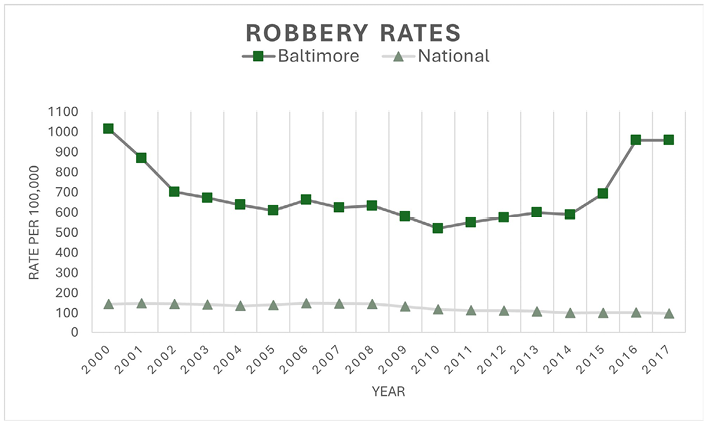
In a study of crime and disorder in Baltimore, the criminologist, Ralph Taylor, noted that crime rates had increased in the second half of the twentieth century, as it had in other large industrial cities in the Eastern US “rustbelt” (Taylor, Reference Taylor2001). Where Baltimore differed from other cities was often in the timing of crime spikes. Unlike other East Coast cities such as New York, Washington, DC, and Philadelphia, where crime rates did not start to spike until the 1980s, crime in Baltimore dramatically worsened in the 1970s, slightly improving in the mid-1980s, to then increase again in 1989 and the early-1990s (Taylor, Reference Taylor2001). Taylor (Reference Taylor2001) summarized robbery rates in the city – in 1970, the city’s robbery rate was 1,200 per 100,000, peaking in 1981 at 1,400/100,000 and then dropping below 1,000/100,000 by the mid-1980s. Associated with the onset of crack cocaine, crime rates started increasing again and the robbery rate reached about 1,700/100,000 in 1992 (Taylor, Reference Taylor2001). Collected from the FBI’s UCR crime statistics, Figure 1.1 shows robbery rates for Baltimore from 2000 through 2017,Footnote 5 and points to the extent of variability of crime rates in the city. In 2000 the robbery rate was at about 1,000 per 100,000 population, much lower than the rate in 1992, but still well above the national robbery rate of 145 per 100,000. By 2010 the robbery rate dropped by nearly half (521 per 100,000) but had again reached above 950 per 100,000 in 2017 compared to the national robbery rate of 98 per 100,000.
Robbery rate for Baltimore compared to national rate, 2000–2017
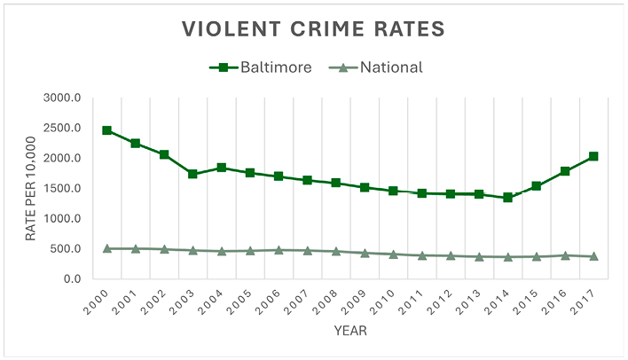
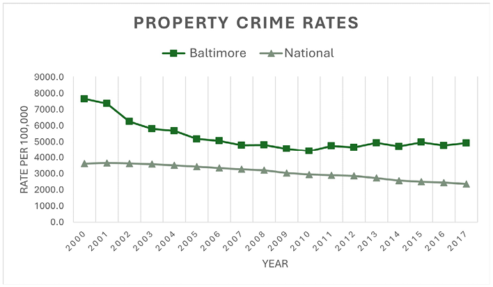
Overall, violent crime rates show a similar trend (see Figure 1.2). For total violent crime, Baltimore’s violent crime rate in the year 2000 was nearly five times the national rate at roughly 2,500 violent crimes per 100,000 compared to a national rate of 500 violent crimes per 100,000. The violent crime rate in Baltimore steadily declined to below 1,400 violent crimes until 2015, when rates started to increase again. In terms of property crime (see Figure 1.3), between 2000 and 2017, the property crime rate was also highest in 2000 (7,662 crimes per 100,000), more than doubling the national average. The property crime rate also started to decline and became fairly stable in 2009, fluctuating between 4,500 and 5,000 property crimes per 100,000, still well above the national property crime rate, decreasing from just over 3,000 property crimes in 2009 to below 2,400 property crimes in 2017. Unlike violent crime rates, Baltimore did not see increases in property crimes between 2015 and 2017.
Violent crime rate for Baltimore compared to national rate, 2000–2017
Property crime rate for Baltimore compared to national rate, 2000–2017
As we describe in more detail below, our study included three waves of data collection conducted between 2013 and 2018. During the second wave in 2015, Freddie Gray Jr. died in police custody and police officers were charged with causing his death. On April 12, Freddie Gray Jr. had been arrested for carrying a switchblade knife and was transported unsecured to a police station. During the transportation in the van, he sustained serious injuries. Video of the arrest showed Gray being “dragged” to a police van “seeming limp and screaming in pain” (Stolberg and Babcock, Reference Stolberg and Babcock2015). After Gray underwent surgery and went into a coma on April 14th, residents began protesting on April 18th, and Freddie Gray died on April 19th because of a spinal injury that occurred while in custody. In the following days, protests escalated to rioting and violence in many parts of the city. We had started collecting surveys and observations only weeks prior to Freddie Gray’s death, and we postponed data collection until May to avoid risk to field researchers and possible hesitancy among residents to participate in the survey. Once the protests subsided and the city curfew was lifted, we started data collection again.
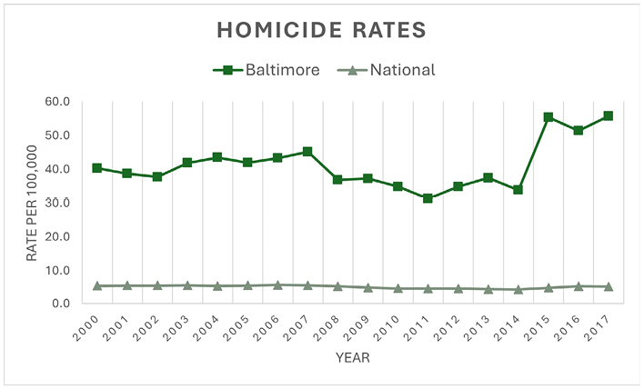
The events did not disrupt the project for a long period of time, but we think it important to note that this was a tumultuous time in Baltimore, and murder rates spiked in 2015, with more than 40 homicides during the month of May alone (Rector, Reference Rector2015). In the summer of 2015, there was a record 45 homicides in July, and a total of 344 homicides for the year, after falling below 200 homicides in 2011 (Rector, Reference Rector2015, Reference Rector2016). Figure 1.4 shows the high homicide rate continued through 2017, the last full year of our data collection. In 2017, Baltimore had the highest homicide rate of any city in the country. We highlight the death of Freddie Gray Jr. and the subsequent riots because we think it important to keep in mind that attitudes of citizens toward the police and crime may have been affected during this period, though as we will see later in the book, there remain strong consistencies in perspectives on crime and policing across our waves of data collection.
Homicide rate for Baltimore compared to national rate, 2000–2017
In studying Baltimore, we also think it important to recognize the degree of abandoned housing and urban blight in the city. In particular, there is evidence of widespread physical disorder in the city, for example, in the number of vacant houses or amount of graffiti (Gunts, Reference Gunts2021; McHugh, Reference McHugh2012; Meehan, Reference Meehan2019; Scott, Reference Scott2022). The number of vacancies dramatically increased during the 90s, from roughly 6,000 vacant homes in 1990 to 8,500 by the mid-1990s (Taylor, Reference Taylor2001). The percentage of streets with at least one vacant dwelling unit increased from 32% in 1981 to 50% in 1994 (Taylor, Reference Taylor2001). Under a new mayor, the city was going to work with community leaders to demolish boarded-up and dilapidated buildings, including entire blocks, for urban renewal, but plans never made it to fruition, and by 2000 there were nearly 14,000 vacant dwelling units (Taylor, Reference Taylor2001). Scandals in public housing and the misappropriation of federal funds meant to provide affordable housing were contributing factors to the deterioration of city housing and living conditions (Pietila, Reference Pietila2010). By 2006, it is estimated that there were over 16,000 vacant buildings. It was only in 2016 that funds would be allocated for demolition efforts (Baltimore City Planning Commission, 2006b; City of Baltimore, 2021; Maryland Department of Housing and Community Development, 2016).
More generally, physical disorder is very high on streets in the city as depicted in the hit television series, “The Wire” on HBO in the early 2000s, with video footage of boarded-up and abandoned row houses accompanied by drug use and poverty. Taylor (Reference Taylor2001) argued that perceptions of dangerousness and incivilities stemmed from the differences between the city, characterized by vacant housing, dilapidated buildings, and graffiti, compared to the surrounding county area, where it was much safer and physical disorder was not present. The widely held view of Baltimore as a disordered city was noted by Donald Trump, who described Baltimore as “the worst city in the U.S.” and a “disgusting, rat and rodent infested mess” where “no one would want to live” (Holcombe, Reference Holcombe2019). At the same time, as we will describe in Chapter 2, our data suggest there is a good deal of variability in physical disorder on the streets we studied, with some streets (especially crime hot spots) with exceedingly high levels of abandoned buildings, graffiti, broken windows, litter or broken glass, and other streets (generally with little crime) evidencing relatively lower levels of such disorder. Abandoned housing and urban blight are more persistent in Baltimore than in many other larger cities in the United States, and that should be kept in mind in considering our findings. But there is also a great deal of variability across streets in the city, and even on higher crime streets. As we illustrate throughout our book, Trump’s description poorly fits what we observed and the way many Baltimore residents feel about their streets and their city.
1.2.1 Understanding Baltimore Crime in Historical Perspective
Of course, to understand why Baltimore ends up among the highest crime cities in the United States, it is important to look a bit closer at its history. Our description in this regard is not meant to be a comprehensive assessment of social and economic trends in Baltimore, for that we refer the reader to a series of other insightful studies (e.g., see Creson, Reference Creson2017; Kelly, Reference Kelly1982; McDougall, Reference McDougall1993; Olson, Reference Olson1997; Taylor, Reference Taylor2001). Nonetheless, the historical context of Baltimore helps us understand how it became a city with high levels of crime and disorder.
Baltimore is located on the East Coast of the United States, and its geography is centered at the Inner Harbor as the downtown district and spreads in all directions away from the harbor, including a small area located across the harbor (see Figure 1.5).
Map of Baltimore City, Maryland
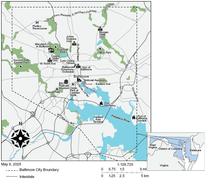
Baltimore, once a 60-acre township grew to 92 square-miles and is located 40 miles northeast of Washington, DC and 100 miles southeast of Philadelphia, PA. With a population of approximately 623,000, the city was the 26th largest city in the United States in 2012 when the study began. The city is home to the N.F.L. team, the Baltimore Ravens, a new franchise started in 1996, and the Baltimore Orioles, a major league baseball team. Oriole Park at Camden Yards, located near the Inner Harbor, was built in 1992 to emulate old baseball parks built in the early 1900s, and has become a major tourist attraction in Baltimore. There are several universities throughout the city of Baltimore, notably Johns Hopkins University founded in 1876, along with University of Maryland, Baltimore (1807), Morgan State University (1867), Coppin State University (1900), and University of Baltimore (1925), among others.
Settled in 1729, Baltimore Town was established in 1730 as a port located at the head of the Patapsco River about 15 miles above Chesapeake Bay. Baltimore was not a major colonial settlement such as New York, Philadelphia, and Boston, and had to make significant efforts to be included in trade and growth. As an early settlement, the town’s main industries consisted of tobacco and grain. The establishment of roads to other cities and shipping routes led to significant growth throughout the late eighteenth century and Baltimore became well-known during the American Revolution for building ships that were exceptional in maneuverability and speed (Olson, Reference Olson1997). Baltimore grew from 564 houses in 1774 to 3,000 in the mid-1790s, and was officially incorporated as a city in 1798 (Olson, Reference Olson1997). Baltimore was also a vital player in the War of 1812 when Britain unsuccessfully tried to capture Fort McHenry, located at the mouth of Baltimore’s Inner Harbor, which was the inspiration for “The Star-Spangled Banner” written in 1814, later to become the U.S. national anthem in 1931.
For the next century, Baltimore continued to grow as waves of immigration, primarily from Germany and Ireland, settled in Baltimore contributing to the city’s diversity and its thriving mercantile economy, eventually transitioning to flour milling, which put Baltimore on the map for trade and commerce around the world. Baltimore made a name for itself in multiple industries including textiles, ship building, copper and steel, and cast-iron, as well as farming and fishery. Alongside growing industries and manufacturing, the arts and sciences also flourished with the growth of the city, and theaters and museums started to emerge. Baltimore also was a leader in the railroad expansion on the East Coast through the establishment of the Baltimore & Ohio Railway Company.
With increasing population, the city struggled to keep up with housing and infrastructure. Roads and housing were built in a tight hierarchical, grid system with housing for different classes in very close quarters, from large homes on main roads, to small homes on the side streets, to alleys that housed laborers and immigrants in tiny houses (Baltimore City Planning Commission, 2006a). As the population grew, so did the city and innovations such as the horsecar railways, steam power, and a city water supply connected neighborhoods and new areas. In 1885, Baltimore was the first U.S. city to establish a commercial electric street railway, further connecting city and suburban areas (Olson, Reference Olson1997). Many suburban areas were incorporated into the city, and between 1850 and 1900, the city grew from 169,000 to 508,957 residents (Baltimore City Planning Commission, 2006a).
Baltimore experienced a devastating fire in 1904 that destroyed much of the city and wiped out the business district. The city was able to quickly rebuild and took advantage of the opportunity to make substantial improvements to the city center, such as the water and sewer systems and underground utilities. Soon after, the city annexed more land in 1918, growing from 30 square miles to almost 90 square miles, roughly the size it is today. Development in these areas looked very different from the inner-city, doing away with alleys, row houses, and the grid layout of streets, for more curved road patterns and single-family homes. This expansion largely excluded Black residents, the population of which grew significantly between 1910 and 1920 as more rural southerners moved to Baltimore. Property taxes were substantially lower in the early suburban developments, while poorer residents in the inner-city continued to pay higher taxes.
The African American community in early Baltimore is notable. In the late 1700s, immigrants from the Caribbean contributed to the growing Black-minority population. In 1820, Baltimore held the largest Black population in the country, with over 26,000 free Black people and roughly 2,000 slaves before the Civil War began. In fact, Baltimore had the largest free Black population of any city in the US at that time (Pietila, Reference Pietila2010). However, even with growing industries, large immigrant populations created competition for jobs, contributing to significantly lower wages and poor living conditions for Black people. While new housing was being developed around the city, this was not the case for Black people, who continued to be crowded into the existing inner-city neighborhoods and small alley houses.
Segregation grew in the early 1900s following the Supreme Court’s Plessy v. Ferguson decision in 1896, and many cities, including Baltimore, developed strategies to exclude Black residents from White neighborhoods and establishments. In 1910, Baltimore was the first city in the country to pass zoning legislation that prohibited Black residents from living in the same neighborhood as White residents, which was enforced down to the street level. This segregation also applied to Jewish immigrants who were excluded from living in White neighborhoods. Major roadways also demarked boundaries to separate neighborhoods and intolerance toward Black residents grew, as more stores, schools, theaters, hotels, hospitals, and cemeteries were separate for White and Black people. In 1917, a Supreme Court decision, Buchanan v. Warley, prohibited residential segregation laws, nullifying Baltimore’s segregation law and supporting property owners to sell real estate to whomever they chose. However, restrictive racial covenants became the tool for continuing segregation.
Baltimore served as a major navy center during World War I, and steelwork, oil refineries, and other war-related industries provided employment opportunities, particularly for unemployed Black migrants moving from the rural south to urban areas for work during the war. Housing availability continued to be a major problem for Baltimore as new homes were not being built fast enough, particularly for the population that was restricted from moving to new homes built in the suburbs. As more housing was being built in the suburban areas, many White residents moved from the inner areas of the city, allowing for the growth of Black and immigrant communities.
Again, the population of Baltimore grew from roughly 558,000 in 1910 to nearly 735,000 in 1920. Throughout the early 1900s, Baltimore’s cultural entities, such as museums and universities, movie theatres and performing arts venues were established. The Baltimore Museum of Art was founded in 1914, the Baltimore Orchestra in 1916, and the Lyric Opera House in 1929.
While the shortage of housing persisted, the Depression exacerbated the problem with the stopping of building of new homes that would persist through World War II as another wave of rural southerners moved to Baltimore to work in the multiple factories that supported the war efforts. Among various industries that supported the war, Baltimore had one of the largest steel mills in the world that provided employment opportunities. Large houses were divided into smaller apartment units and multiple beds were put in row houses for the workers, while White residents continued to move to the suburbs and surrounding counties (Olson, Reference Olson1997).
Baltimore’s population peaked at around one million people in 1950 and then started to steadily decrease as suburban living became more popular, and as people moved away, industries and employment opportunities followed. During the first half of the century, Black residents comprised around 16–19 percent of the city’s population, which began to steadily increase over the next several decades. This was also during the time when practices such as redlining and blockbusting were becoming increasingly more popular as ways to maintain racial segregation.Footnote 6 Blockbusting went hand in hand with a practice called “land-installment contracts.” Since banks would not provide mortgage loans to Black residents or loans for building houses for Black people more generally, landlords used land installment contracts that provided a way for residents to rent homes with an option to buy, but it also took advantage of tenants. The practice was targeted toward Black residents who aspired to own homes, but was highly abusive as slumlords charged higher than market-value rent, included multiple fees, and charged tenants costs for repairs, and rarely would the tenant end up actually owning the home (Olson, Reference Olson1997; Pietila, Reference Pietila2010). At the same time, White residents, fearing integration, would sell their homes for less than market-value. Multiple studies have confirmed that Black families paid more than White families for the same housing in Baltimore while earning significantly less income (Olson, Reference Olson1997). While blockbusting and land-installment contracts had a negative financial impact on Black (and Jewish) residents, it provided an opening for residents to move into historically White neighborhoods. Though once a Black or Jewish family moved onto the block, White residents often moved out – the “White flight” was markedly apparent (Orser, Reference Orser, Fee, Shopes and Zeidman1991).
Another significant point in Baltimore’s history was the Riots of 1968 following the assassination of Martin Luther King, Jr. With Baltimore being more than 40 percent Black at that time, the Civil Rights Movement was strong in Baltimore, with many prominent leaders, and when Martin Luther King, Jr. was killed, there was widespread rioting, burning of buildings, looting, and violence. Over the course of three days over 5,000 people were arrested, thousands of houses and businesses were destroyed, 700 people were injured and 6 people died (Pietila, Reference Pietila2010, p. 196). Like many cities throughout the U.S., the National Guard and army troops were called in to patrol the city. The Civil Rights Act of 1968 was passed within eight days of Martin Luther King, Jr.’s assassination, outlawing redlining and including a provision for fair housing which “outlawed discrimination based on race, religion, national origin, and gender in the sale, rental, and financing of housing” (Pietila, Reference Pietila2010, p. 197). While this legislation ended legal segregation and diminished much of the discrimination in housing, it did not stop banks from moving out of the inner-city and favoring home loans in the suburban areas of Baltimore (Gomez, Reference Gomez2013).
While Baltimore was experiencing rapid racial changes in neighborhoods, the city was also adapting to modern urbanism with significant improvements and urban renewal. The renowned Charles Center was built between 1958 and 1962 that consisted of office buildings, residential towers, a hotel, movie theater, and new retail outlets across several city blocks. This was followed by redeveloping the Inner Harbor in the 1970s to provide multiuse purposes and several attractions for tourism in the city. The B&O Railroad Museum, highlighting Baltimore’s significant role in railway development opened in the early 1950s with significant innovations and restorations made in the 1970s. The National Aquarium broke ground in 1978, gaining “national” recognition by Congress in 1979 and opened to the public in 1981. Today it is the only National Aquarium in the U.S., as the Washington DC aquarium closed in 2013. The Inner Harbor is also home to a Civil War-era ship, the USS Constellation built in 1854, where it is docked as a museum ship and classified as a National Historical Landmark. Under Baltimore’s first Black mayor, William Donald Shaefer (1971–1986), these renovations and growth in urban development earned Baltimore the nickname of “Renaissance City” in Time (Olson, Reference Olson1997); however, school budgets were being cut and there was significant population loss in the city during this time. The city population dropped below 700,000 and the region lost over 90,000 factory jobs between 1970 and 1995 (Olson, Reference Olson1997).
During this period, the city transitioned from a majority White residents to majority Black residents, and by 1980, the city was roughly 55 percent Black residents. The growing income gap and isolation of inner-city communities greatly impacted the safety of Baltimore neighborhoods, not only in terms of crime, but also in the unsanitary living conditions of homes and neighborhoods. Neighborhoods that once experienced severe housing shortages in the 40s and 50s, were becoming increasingly more vacant. Many neighborhoods, often dominated by Black residents, were now hot beds for drug addiction, HIV/AIDS, and violence (Olson, Reference Olson1997). In the 1960s, the illegal drug industry was growing among younger people, and homicide and suicide rates began to increase, with a combined rate of a thousand deaths per year in the late 60s (Olson, Reference Olson1997). With some of the highest AIDS/HIV rates in the country, since the epidemic started in the early 1980s, Baltimore recorded 4,000 deaths due to AIDs in 1996, 2,900 people had symptoms of AIDS and another 12,000 were living with HIV infection; in some Black neighborhoods, the rates were as high as 1 in 10 persons infected with HIV (Olson, Reference Olson1997, p. 399). The spread of this disease can be attributed to injection of drugs, which were also a contributing factor to juvenile crime and violence that was also increasing in the early 1990s.
The first decade of the twenty-first century was a period of optimism and development in Baltimore. In a brochure published by the city in 2005, Baltimore government could claim that it led the “big cities in reducing crime,” and noted that violent crime was at its “lowest level since the 1960s” (Baltimore City Department of Planning, 2006a). The brochure noted that “(o)ur first and second graders are scoring above the national average in reading and math for the first time in 30 years … and three of our high schools are ranked among the State’s top ten and each year more students are graduating from our high schools.” The brochure acknowledged that “stubborn urban ills still plague Baltimore,” and noted that the city had “been scorched by devastating fires, real and figurative,” but stated optimistically that from “these ashes, Baltimore, once again, is rising.” Indeed, as we illustrated earlier, at least in terms of crime, in the first decade and a half of the twenty-first century crime rates had improved substantially. But many of those gains appear to have been lost after 2015 with the death of Freddie Gray in police custody and subsequent rioting in the city.
1.3 The Study
As we noted earlier, until our study, there was almost no systematic knowledge about the people who live in crime hot spots. Adding complication to providing such descriptions, there has not been consensus among researchers about the geographic unit that should define a micro geographic crime hot spot. Some authors have looked at specific addresses with high numbers of crimes (Pierce et al., Reference Pierce, Spaar and Briggs1988; Sherman et al., Reference Sherman, Gartin and Buerger1989), others have focused similarly on facilities such as stores or factories (Eck et al., Reference Eck, Gersh, Taylor, Goldsmith, McGuire, Mollenkopf and Ross2000). Still others have focused on clusters of streets, which are characterized by similar crime problems (Bernasco and Block, Reference Bernasco and Block2011; Haberman et al., Reference Haberman2017). Often the definition of a hot spot is driven by a particular crime prevention program, or the focus of police or other prevention agents.
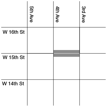
We define the geographic unit of our study as the street segment, which includes both sides of the street between two intersections (see Figure 1.6). We chose the street segment for a variety of theoretical and operational reasons. In geographic terms, it is a very small building block from which to examine hot spots of crime. At the same time, it is a social unit that has been recognized as important in the rhythms of everyday living in cities. It is important to note that street segments are different from street blocks defined by the US census. Street blocks include all four block faces extending around a “block” which means that block faces that face each other on the street are not part of the same micro geographic unit (see Figure 1.6, 15th St. between 4th and 3rd Ave.). A key criterion for defining hot spots in our study is that they form social as well as geographic units, so a census block, which separates two block faces immediately across from each other, was not an appropriate geographic unit for our study.
Visual of street segment
Theoretically, scholars have long recognized the relevance of street segments in organizing life in the city (Appleyard, Reference Appleyard1981; Brower, Reference Brower, Altman and Werner1980; Jacobs, Reference Jacobs1961; Taylor et al., Reference Taylor, Gottfredson and Brower1984; Unger and Wandersman, Reference Unger and Wandersman1983). Ecological psychology, in particular, has attempted to understand how places function as social units (Barker, Reference Barker1968; Wicker, Reference Wicker, D. Stokols and I. Altman1987). From his observations of places, Barker developed “behavior settings theory.” Wicker (Reference Wicker, D. Stokols and I. Altman1987) defines behavior settings as “small-scale social systems whose components include people and inanimate objects.” He goes on to say that “within the temporal and spatial boundaries of the system, the various components interact in an orderly, established fashion to carry out the setting’s essential functions” (Wicker, Reference Wicker, D. Stokols and I. Altman1987, p. 614).
Weisburd et al. (Reference Weisburd, Groff and Yang2012) following Taylor (Reference Taylor1997, Reference Taylor, Taylor, Bazemore, Boland, Clear, Corbett, Feinblatt, Berman, Sviridoff and Stone1998), made the case for why street segments function as behavior settings.Footnote 7 First, people who frequent a street segment get to know one another and become familiar with each other’s routines. Second, residents develop certain roles they play in the life of the street segment (e.g., the busybody, the organizer, the dogwalker). Consistency of roles increases the stability of activities at places. On many streets, for example, there is often at least one neighbor who will accept packages for other residents when they are not at home. Third, norms about acceptable behavior develop and are generally shared. Shared norms develop from interactions with other residents and observations of behaviors that take place on the street without being challenged. Fourth, streets have standing patterns of behavior that are temporally specific. The mail carrier delivers at a certain time of day, the corner resident is always home by 5 pm, another neighbor always mows the lawn on Saturday. Fifth, a street segment has boundaries that contain its setting. It is bounded by the cross streets on each end. Interaction is focused inward toward the street. Finally, street segments, like other behavior settings, are dynamic. Residents move out, and new ones move in. Land use could shift as residential units become stores at the street-level and remain residential on the upper floors. These types of changes to the social and physical environment of the street segment can alter the standing patterns of behavior.
Beyond the theoretical justification for using street segments to understanding crime and place, there are other advantages. Unlike neighborhood boundaries, street segments are easily recognized by residents and have well-defined boundaries (Taylor, Reference Taylor, Taylor, Bazemore, Boland, Clear, Corbett, Feinblatt, Berman, Sviridoff and Stone1998). Moreover, the small size of street segments minimizes spatial heterogeneity and makes it easier to link characteristics of street segments to outcomes such as crime (Rice and Smith, Reference Rice and Smith2002; Smith et al., Reference Smith, Frazee and Davison2000). In turn, scholars have argued that informal social control and territoriality (Taylor et al., Reference Taylor, Gottfredson and Brower1984) are more effective in smaller settings such as street segments. Operationally, the choice of street segments over even smaller units, such as addresses (see Sherman et al., Reference Sherman, Gartin and Buerger1989), also minimizes the error likely to develop from miscoding of addresses in official data (see Klinger and Bridges, Reference Klinger and Bridges1997; Weisburd and Green, Reference Weisburd, Green, MacKenzie and Uchida1994). We recognize however, that crime events may be linked across street segments. For example, a drug market may operate across a series of blocks (Weisburd and Green, Reference Weisburd and Green1995; Worden et al., Reference Worden, Bynum, Frank, Mackenzie and Uchida1994), and a large housing project and problems associated with it may transverse street segments in multiple directions (see Skogan and Annan, Reference Skogan, Annan, MacKenzie and Uchida1994). Nonetheless, we thought the street segment offers a useful compromise because it allows a unit of analysis large enough to avoid unnecessary crime coding errors, but small enough to avoid aggregation that might hide specific trends.
Our use of the street segment as a unit of analysis follows numerous studies that examine crime concentrations and crime hot spots at the micro geographic level. Weisburd et al. (Reference Weisburd, Groff and Yang2012) used street segments in their longitudinal study of crime at place in Seattle (also see Weisburd et al., Reference Weisburd, Bushway, Lum and Yang2004). Additionally, studies conducted not only in North American cities but also in countries across Europe, Latin America, and Africa have frequently used street segments as the unit of analysis for examining crime concentrations (e.g., see Andresen and Linning, Reference Andresen and Linning2012; Bernasco and Steenbeek, Reference Bernasco and Steenbeek2017; Chainey et al., Reference Chainey, Pezzuchi, Guerrero Rojas, Hernandez Ramirez, Monteiro and Rosas Valdez2019; Chalfin et al., Reference Chalfin, Kaplan and Cuellar2021; Gill et al., Reference Gill, Wooditch and Weisburd2017; Steenbeek and Weisburd, Reference Steenbeek and Weisburd2016; Theron et al., Reference Theron, Breetzke, Snyman and Edelstein2023). Indeed, a recent review of crime concentration research finds street segments to be the most common geographic unit in research defining crime concentrations in cities (Weisburd, Zastrow, et al., Reference Zastrow2024).
1.3.1 Sampling Hot Spot and Non–Hot Spot Streets
The sampling for the study began with the full population of 25,045 street segments in Baltimore, and CFS data from the Baltimore Police Department (BCPD) for 2012 were geocoded (match rate = 98.8 percent) to create aggregate counts of violent crime (rape, robbery, bank hold up, aggravated assault, common assault, carjacking, abduction, and sniper) calls and drug crime (narcotics, narcotics outside, and narcotics on-view) calls (see Chapter 1 Appendix for an exhaustive list of included call types). We used “crime calls to the police” because we wanted to include a broad measure of crime that was less filtered by police decision-making. Crime incidents, which are more often used for estimating crime levels in studies of police interventions, involve police “founding” or identifying a reported crime as reflecting an actual crime event.Footnote 8 Most crime calls are generated by citizens calling the police.Footnote 9 But crime calls are also created when the police observe suspicious activity that they believe might be a crime and call in to the dispatcher that they are responding.
Our goal was to identify a sample of 450 street segments in which there would be a larger sample of crime hot spots (about 2/3rds) and a comparison sample of streets that were not hot spots. We conducted statistical power analyses to ensure that this sample size of streets would allow for statistically powerful tests of our main hypotheses. We wanted to be confident that we had a large enough sample to examine differences between hot spot and non–hot spot streets.
A key criterion for our study was that the streets we examined were residential streets. We wanted to be able to talk about how people on high-crime streets experienced those streets, and because of this, we excluded exclusively commercial streets from our study.Footnote 10 We also restricted our sample streets to residential streets with a minimum of twenty occupied addresses. This threshold was created because we wanted a large enough sample of people on each street that we could gain reliable portraits of characteristics of streets in the study, for example, whether streets were characterized by high levels of people willing to intervene on problems on the street or trust their neighbors, or by high levels of mental or physical health problems, or whether streets had more residents with high school educations, or who were employed.
Because there is a finite population of households on each street segment, we had to consider the likely response rate of a survey in relation to this finite population, to identify whether it would be possible to include enough responses on each street. Assuming a response rate of 35 percent, a minimum population of 20 or more occupied households on the street was likely to yield about seven surveys.Footnote 11 We believe that this sample goal represented a useful compromise between the loss of sampling frame, or street segments available to study, and the sample size needed to describe street-level characteristics. We used a database from the Baltimore Mayor’s Office for 2010 to determine occupied housing on Baltimore streets, though as we note below, we also corrected these totals based on observations by our research team. This criterion reduced the sampling frame from over 25,000 streets to 4,630 street segments for study.
Crime hot spots were defined as streets that were in the top 3 percent for violent- or drug-related calls for service in order to assure a sample of very high-crime streets.Footnote 12 Three categories of crime hot spots were created – drug crime hot spots, violent crime hot spots, and combined violent drug hot spots (those streets that met a minimum threshold for both drug and violent crime calls). Hot spot street segments were then sampled from the three categories of crime hot spots through a random sampling procedure developed in Model Builder (in ArcGIS) that prevented any two sampled streets from being within a one-block buffer area. Once the sample of residential street segments was selected, field researchers conducted a physical census of each street segment to identify any unusual barriers that would alter the street segment setting (e.g., bridges, alleys), and to confirm the street met the criterion for occupied dwelling units.Footnote 13 If a street segment did not meet the sampling criteria after the census, streets were replaced as needed to reach the sample goals. A comparison group of “non-hot spot” street segments was sampled following the same procedures carried out for the hot spot street segments. Based on a review of the distribution of crime calls on these “non-hot spot” streets, the non–hot spot streets were further divided into “cold” spots (three or fewer crime calls for service for drug or violent crime) and “cool spots” (four or more calls for service for drug or violent crime, but less than the threshold for a hot spot). The final sample of street segments in the study consisted of 46 cold spots, 100 cool spots, 120 drug hot spots, 126 violent hot spots, and 55 combined drug and violent crime hot spots.Footnote 14
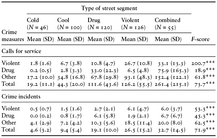
Looking at the average number of violent and drug crime calls for service and crime incidents (see Chapter 1 Appendix for crime categories included) for each street type presented in Table 1.1, we can see both the very high rates of crime calls and incidents that hot spot streets exhibited, as well as the large differences between hot spots and non–hot spots, and especially between hot spots and cold spots. While cold spots evidenced on average only 2 drug and violent crime calls and cool spots about 10 drug and violent calls, drug hot spots averaged 44 drug and violent calls, violent crime hot spots 33 drug and violent calls, and the combined hot spots about 110 calls for violent or drug crime during the selection year. Reinforcing their identification as crime hot spots, drug hot spots, and violent crime hot spots had on average 112 and 126 total calls for crime in the selection year, and combined hot spots averaged over 260 calls. Total crime incidents averaged about five for cold spots and nine for cool spots. In crime hot spots, the average number of crime incidents is nineteen for drug hot spots, twenty-seven for violent hot spots, and thirty-three for combined drug and violence crime hot spots.
Note:
*** p < 0.001.
We recognize that the over-sampling of crime hot spots leads to a sample of places that includes a much larger number of hot spots than would be included had the study randomly sampled streets from the full population of street segments. At the same time, it is important to recognize that many residential streets in the city do not have serious crime problems. Fully 86.4 percent of the population of residential streets sampled in the study did not meet the criteria for a hot spot, meaning that if the streets had been sampled randomly, only a small number of crime hot spots as we define them would have been included in the sample. Given our desire to describe the social structure and social context of hot spots of crime, this overrepresentation is planned and allows us to study hot spots in a way that would not be possible had we randomly sampled streets in the city.
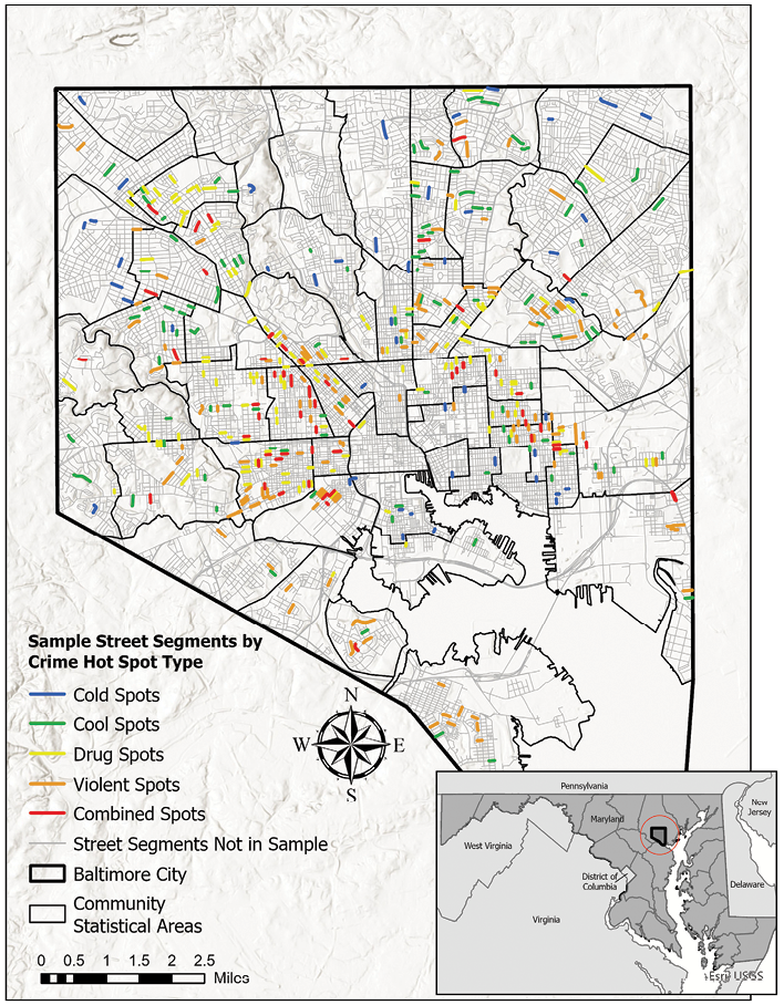
As shown in our map of Baltimore (Figure 1.7), the five street segment types appear to be spatially heterogeneous, though the crime hot spots are somewhat more likely to be located in the central areas of the city, to the east and west of the inner harbor. This is not surprising given our short history of Baltimore, where segregation and other social policies pushed minority and disadvantaged populations into the inner-city, while better off White residents moved away from the city center and often into the suburbs.
Map of sample street segments by crime hot spot type in Baltimore City, Maryland
1.3.2 Survey Interviews of Residents Who Lived on the Study Streets
Perhaps the most important data we collected for describing the social structure and social context of street segments in our study were drawn from surveys of community members. Here we asked large numbers of residents on our sample streets about their perceptions on a range of issues, including: crime and disorder on the streets, fear of crime, their trust of their neighbors and willingness to intervene in problems, their experiences on the streets with police and crime, their economic, educational and social circumstances, as well as questions about their substance use, smoking, drinking behavior, and physical and mental health status. The survey included 146 questions (and over 300 unique items), and was conducted face-to-face using Scantron bubble forms that the field researchers read to the participant and filled in with the responses provided by the respondent. The survey took an average of 20–25 minutes to complete, and respondents were compensated $15 for their participation.
We carried out three waves of survey data collection in the study: the first between August 2013 and June 2014; the second wave between April and December 2015, and wave 3 was carried out between April 2017 and March 2018. Residential dwelling units were randomly sampled, and trained field researchers interviewed the first adult resident contacted (twenty-one years or older), who had lived on the street for at least three months. The contact rate, which measures the proportion of people we were able to reach to ask to participate in the survey, was 71.2% in the first wave, 80.0% in the second wave, and 87.9% in the third wave. The cooperation rate, or the proportion of people we contacted who participated in the survey was 60.5% in wave 1, 71.6% in wave 2, and 58% in wave 3. These are above average results for door-to-door surveying (Babbie, Reference Babbie2020; Holbrook et al., Reference Holbrook, Krosnick and Pfent2008).
The survey was a massive endeavor for the research team, and there could be as many as 60 field researchers employed at the same time during each wave of data collection. Teams of three to four field researchers,Footnote 15 including a team leader, visited street segments between the hours of 11 am and 8 pm, seven days a week across the study period. In wave 1, interviewers returned to dwelling units an average of four times and up to twenty-five visits. In wave 2, the teams visited the dwelling unit an average of 6.3 times, with up to 32 visits. In wave 3, the number of visits to the streets ranged from 2 to 27 visits, with a mean of 13 visits to the streets. Dwelling units where a survey was not completed were visited an average of eight times (at which point we resampled a new dwelling unit if no contact was made), but we continued to visit these dwelling units over the course of the study unless a hard refusal was made by a resident of the dwelling unit. When residents were not available to complete the survey at that time or the identified adult from a previous wave was not at home, interviewers scheduled timeframes or appointments to return to the household to complete the survey.
An important part of our planning of the survey data collection, and other field research on the sampled streets, was ensuring the safety of data collectors. Working in hot spots of crime can be dangerous. In our study we had multiple events of shootings on the hot spot streets we visited, and during the Freddie Gray riots, one research team had their windshield broken by a brick thrown by rioters. We developed several safety protocols for procedures for working in dangerous or high-risk conditions in the field, which are available in our online resources.
In wave 1, a total of 3,738 surveys were completed, 3,615 were completed in wave 2, and in wave 3, a total of 3,141 surveys were completed, for a total of 10,494 eligible surveys across the three waves.Footnote 16 With the exception of six streets in wave 1 and one street in wave 2, we completed at least 7 surveys on each street segment. In wave 3, 87.2 percent of sample street segments had seven or more surveys.
1.3.3 Physical Observations
A key set of indicators for our study was the physical attributes of the street. The survey asked about such attributes, but we also wanted a measure that was objective in the sense of researchers observing the street. Physical observations are particularly important in our study because of perspectives like Broken Windows theory (see Wilson and Kelling, Reference Wilson and Kelling1982; Kelling and Coles, Reference Kelling and Coles1996), which view physical decay as an important factor in understanding and predicting crime.
Our physical observations were conducted simultaneously during survey data collection.Footnote 17 For each of the street segments, two trained observers rated the discrete characteristics of the street segment independently in order to test for and periodically monitor inter-rater reliability. The observers went to each street during the period of the survey data collection, but not when other research activities were being carried out. Field researchers spent between ½ hour and an hour carefully coding the physical attributes of the street and moved to multiple viewing areas along the street to accurately code the observation items.
The physical observation instrument had four separate focus areas to capture several dimensions of the street environment, including known ecological risk factors for antisocial behavior (e.g., bars and bus stops). First, the number of buildings and physical structures on the street were documented along with the use or purpose of the buildings, such as residential, commercial, and public service. Next, there were several observational items related to physical disorder, such as visual indicators of drug activity (drug paraphernalia) and prostitution (e.g., condoms on the street), as well as broader signs of physical disorder, such as burned-out or abandoned buildings, litter, graffiti, broken windows, structural damage, and abandoned vehicles. Lastly, measures of the physical design and conditions of the street were captured such as construction on the street, number of street lanes and alleys, and the presence of security cameras, benches, and bus stops.
1.3.4 Systematic Social Observations
Systematic social observations were conducted only in the first wave of data collection between April and June of 2014.Footnote 18 These observations were aimed at measuring various types of social activities and the volume occurring in public places using a structured observation protocol. Each street segment in the sample received three systematic social observations, each lasting for 20 minutes. To observe the street at different days of the week and times of day, one observation occurred during weekday hours (10:00 am–4:00 pm), one observation during weeknight hours (4:00 pm–8:00 pm), and one observation occurring on the weekends (10:00 am–8:00 pm), resulting in over 1,300 systematic social observations. Each observation provided a snapshot of the social conditions of the street with the presence of different activities and external conditions on the street segment, while also capturing the amount of time specific events occurred on the street.Footnote 19
Similar to the physical observations of the street, field researchers worked in pairs, and during the first visit to the street segment, the team identified a location on the street where the greatest amount of social activity could be observed, an “epicenter” of the street. This location remained the same for all subsequent visits to the street, and field researchers generally stayed at this spot for the entire observation period unless something obstructed their view, or they felt concerned about their personal safety or well-being (in which case they left the street).
One field researcher focused on providing a “snapshot” of the street, recording the presence of indicators of social disorder and antisocial behavior such as people arguing, loitering, or drug activity; prosocial activities such as recreation, children at play, adults working on their home and yards; and levels of pedestrian activity (including some characteristics of the people), traffic, and noise on the street. The other field researcher focused more closely on specific activities taking place and their duration, by timing each event they observed, and the number of people involved. Some of these activities included soliciting sex, public drinking, drug selling and use, and gambling, as well as certain types of people providing guardianship on the street like place managers (e.g., a business owner or security officer), police officers, or healthcare providers.
1.3.5 Qualitative Data Collection
During each wave of survey data collection, qualitative data collection including ecological mapping,Footnote 20 direct observation of street segments (including the businesses, individuals, and groups within them) and in-depth, semi-structured interviews were conducted. The use of multiple methodologies triangulates the data sources, offering greater depth and reliability in the results (Lofland et al., Reference Lofland, Snow, Anderson and Lofland2006; Morrill, Reference Morrill1995; Snow and Anderson, Reference Snow and Anderson1993). Qualitative data is particularly suited to developing a deeper understanding of how people who live, work, and visit these streets understand their social context. In the chapters that follow, we often use qualitative narratives as a way of illustrating and contextualizing our quantitative findings. During wave 1, we spoke with 72 individuals across 42 interviews; in some instances, we spoke with small groups (2–4 individuals) on the street. In wave 2, the field researchers conducted 86 interviews, again, some were with small groups, for a total of 103 individuals interviewed. And in wave 3, 71 individuals were interviewed across 60 interviews.
Qualitative methods included ethnographic observation and informal interviewing of residents or occupants of each street segment during fieldwork. The qualitative research team spent roughly an equal time developing their field notes as they did in the field. During fieldwork, researchers spent one hour on each street segment in the qualitative subsample, gathering observational and interview data to understand – How do residents view, use, and perceive the street segment? Within each street segment, we maximized diversity in the recruitment of individuals by speaking with and providing study information sheets to all eligible residents and inhabitants. While paying attention to local demographics (i.e., age, race/ethnicity, and gender), we interviewed individuals based on the following inclusion criteria: (1) at least twenty-one years old; (2) present on street segment during fieldwork; (3) voluntarily participates. Rather than engaging in formal interviews (with interview questionnaires/protocols), we used direct observation time for conducting semi-structured interviews (thematically focused interviews that occur during the course of everyday conversation). We engaged participants in conversations to delve for information using Snow and Anderson’s “interviewing by comment” procedure for eliciting information by making a statement that sparks response (Snow and Anderson, Reference Snow and Anderson1987).
1.4 What Follows
The comprehensive data collection we have just described allows us to develop a more comprehensive picture of hot spots of crime than any prior study. And it allows us to compare hot spots of crime with what we have termed cool and cold spots, as well. In the chapters that follow, we use these data to answer a series of questions about the social structure and social context of crime hot spots and their relationship to crime, victimization, and health. Our work seeks to bring social structure and social context into scholarly and policy discussions of hot spots of crime.
Chapter 2 provides a descriptive portrait of hot spots of crime, focusing in particular on social disadvantage and social disorganization across hot spot and non–hot spot streets in our study. We also examine characteristics of hot spots that are often seen as tightly linked to crime, such as social and physical disorder and fear of crime. As we describe in this chapter, while hot spots of crime are characterized by high levels of concentrated disadvantage, low informal social controls, high levels of social and physical disorder, and an elevated fear of crime, these are places that also have strong social ties among neighbors, and they include residents that hope that their streets will improve. Chapter 3 builds on this foundation by exploring whether the differences between hot spot and non–hot spot streets vary based on the type of community they are nested in, categorized by levels of concentrated disadvantage. It also investigates how the characteristics of hot spot streets differ depending on the broader community context in which they are situated. We find that hot spots of crime in very different types of neighborhoods have many similar characteristics, but that the community context also influences characteristics of crime hot spots.
Chapter 4 expands upon prior research on crime hot spots, which has primarily focused on opportunity-related factors that explain crime, by showing that social context, particularly informal social control, also plays a crucial role in understanding crime at place. Our models add strong evidence to the idea that we need to consider social context in understanding the emergence of crime hot spots. Because of the very strong impact of informal social control on crime, in Chapter 5 we examine specifically what influences informal social control on streets. This is particularly important given criminological work that has focused on physical and social disorder as impacting informal community social controls. Our findings suggest that the focus on physical disorder for increasing levels of informal social control may be misplaced, though we also show that social disorder is an important influence on informal social controls at crime hot spots.
Chapter 6 illustrates that the social structure and social context of streets matter not only for understanding crime but also for understanding the risk of property crime victimization experienced by residents, even after accounting for individual lifestyles. Chapter 7 demonstrates that the health conditions of residents in crime hot spots constitute another critical dimension for understanding the broader social context of these places. Compared to non–hot spots, residents of crime hot spots exhibit higher rates of physical and mental health problems, with this geographic overlap between crime and health risks being at least partially attributable to the living conditions on those streets.
Finally, Chapter 8 concludes the book by summarizing our key findings and discussing their implications for theory and policy. Together, these chapters suggest that it is important to bring the social structure and social context of hot spots of crime into our understanding of why these places have high rates of crime, and what types of interventions are likely to help ameliorate crime and related problems at crime hot spots.
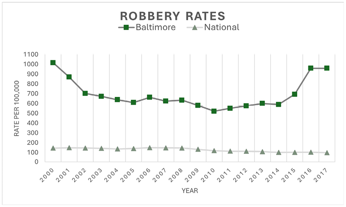
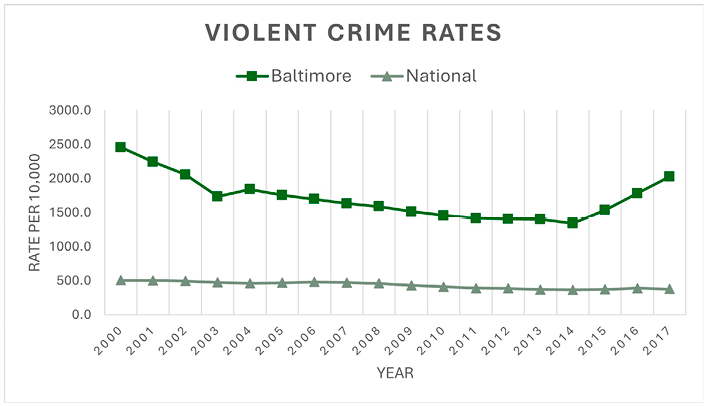
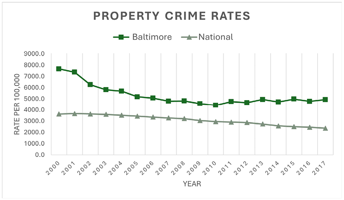
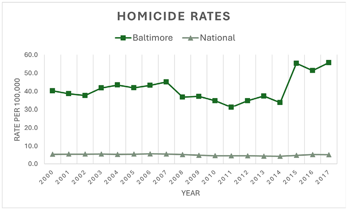
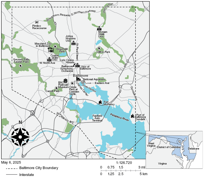
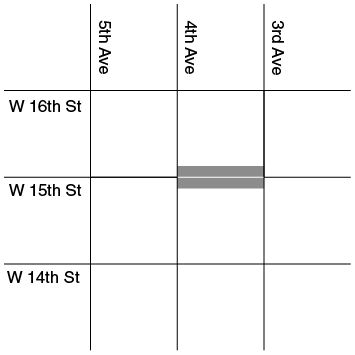
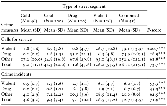
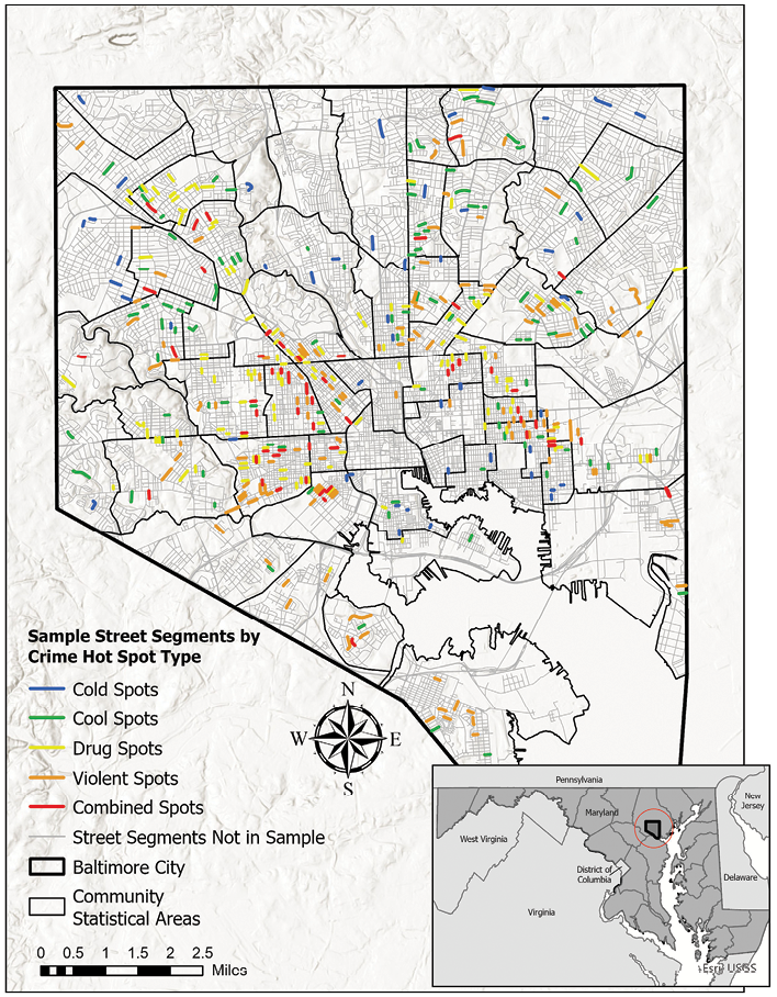

 Open access