

1. Introduction
Observations of large numbers of icebergs in the waters around Antarctica have been ubiquitous from the first days of exploration of the continent. The early explorers, the seal and whale hunters, and the later research expeditions all reported many icebergs, including giant tabular icebergs. But such observations were not adequate to assess the total magnitude of icebergs, the extent iceberg calving played in the mass balance of the Antarctic Ice Sheet or whether there were changes in iceberg quantities over time. While there had been various reports detailing iceberg sightings (Dmitrash, Reference Dmitrash1965, Reference Dmitrash1971; Romanov, Reference Romanov1975), systematic recordings in the 1978/1979 summer season between Cape Town and the southern Weddell Sea on M/V Polarsirkel indicated that the earlier reports from the coastal waters of East Antarctica were not representative (Orheim, Reference Orheim1980). The numbers of icebergs reported were small and the sizes recorded were large, thus smaller icebergs and total numbers seemed seriously under-reported. An international program for the systematic collection of Antarctic iceberg data was therefore initiated in 1981 by the Norwegian Polar Institute (Norsk Polarinstitutt, NPI), motivated by this lack of data on the spatial and temporal distribution of icebergs in Antarctic waters.
The program was endorsed by the Scientific Committee on Antarctic Research (SCAR) through its Working Group on Glaciology, and quickly gained support from nearly all SCAR nations. Already by the 1982/1983 austral season, most ships active within Antarctic waters carried standardized reporting instructions with what became known as the ‘Blue Forms’ (Fig. S1, Table S2) on which the iceberg observations were recorded. The distribution of the ‘Blue Forms’ ceased after the 2000/2001 season, but data continued to be collected until the 2009/2010 season (Tables S3, S4). During the three decades of observations, most of the ocean around Antarctica was observed, but there were large differences in data density, primarily because nearly all ship tracks follow repeated routes to the various research stations, and these are not evenly distributed around the continent. The NPI database makes up ~80% of what we present here as the SCAR International Iceberg database. The remaining ~20% consists of observations collected by Australian National Antarctic Research Expeditions (ANARE) operating in the 50–150°E longitude sector.
The strength of the present database is the large number of observations using identical recording protocols for standard iceberg sizes, providing systematic coverage over most of the waters around Antarctica. These data provide a solid, long-term record of Antarctic iceberg sizes, movement and distribution before the era of polar orbiting satellites and on-board remote sensors, along with inferred calculations of dissolution rates, ocean currents, etc., upon which future remotely sensed iceberg data can be compared and tested. We discuss the iceberg observations in comparison with newer satellite data. The ship-based data are particularly useful because they include systematic observations of smaller icebergs not covered by satellite-based databases.
2. Data and methods
2.1. Collecting the NPI data
Instructions for the ship-based observations were distributed to all nations having an Antarctic research program, as indicated by the membership of COMNAP (Council of Managers of National Antarctic Programs). The ‘Blue Form’ instructions (Fig. S1) started by defining an iceberg as ‘a large mass of floating or stranded ice of greatly varying shape, more than five metres above sea level, which has broken away from a glacier or ice shelf’. It was requested that observations be made every 6 h at the times of standard meteorological observations, and that recordings start immediately after port departure, or after crossing 40°S, even though no icebergs might then be seen. In practice, many records started further south since they commenced with the first sighting of an iceberg. The 6 h interval was chosen primarily because it provided a task load on the staff on the bridge that was acceptable for a voluntary assignment. This interval also gave reasonable statistical coverage, as it meant that a moving vessel would normally not make duplicate observations.
The instructions asked that all icebergs be recorded within five size classes according to observed horizontal dimension: 10–50, 50–200, 200–500, 500–1000 and >1000 m. Additional information such as freeboard, width and breadth was requested for the largest size class. The extent to which the latter was done varied from observer to observer. The choice of five size classes was based on initial experiences of asking bridge personnel to carry out such observations, which indicated that recording five classes was not too laborious. In order to make the classification easier, page two of each form gave a diagrammatic scheme showing which size class an iceberg would fall into, given an angular extent measured by sextant combined with distance measured by radar. In fact, the apparent horizontal dimension of a tabular iceberg recorded from afar will depend on the shape of the iceberg and its alignment to the observer, and it will be between the longest dimension (diagonal for a rectangle) and the width, depending on the alignment. Although observers were requested to classify the icebergs by size, this was not always possible. Most often, this was due to low visibility so that the number of icebergs was counted by radar without size being determined. In some cases, only estimated counts were recorded when many icebergs, sometimes exceeding 100, were present in the smallest category. Additionally, the observer noted ship position, date and time of observation, sea-ice concentration and information on whether the observation was made visually or by radar.
The number of ships contributing to the dataset increased with time and reached a maximum in 1987/1988, when data were recorded on more than 20 cruises. The number of ships sending reports thereafter gradually decreased until the 2000/2001 season, as personnel changes meant that NPI provided less support and follow-up. New forms were not sent out after 2000 but some countries continued to submit data using remaining ‘Blue Forms’ or copies observers had made. All these later data reports are also included here, until the program was formally terminated in 2012. It was then decided that the accumulated dataset should be published in a format making it available to other researchers. For that to happen the data were scrutinized once more to, as far as possible, eliminate human error. The full NPI database contains 26 601 observations, comprising 320 493 icebergs, giving an average observation of 12 icebergs. Altogether 259 479 icebergs were classified by size, distributed in the five classes as shown in Table 1. This report describes the complete dataset, together with its uncertainties, and suggests various results that can be derived from the observed distributions in space and time. The SCAR database can be downloaded at https://doi.org/10.21334/npolar.2021.e4b9a604 and is available in CSV file formats.
The number and percentage of icebergs observed in each of five size classes. The table shows all NPI data, which include the pre 1984/85 ANARE data.

2.2. Collating the ANARE data with the NPI data
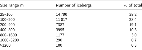
The Australian Antarctic Division (AAD) has routinely collated data on iceberg location and size since 1948 from ANARE ships mostly operating in the 50–150°E longitude sector, but a more rigorous data collection routine was initiated in 1977. More recently, a joint program between NPI, AAD and the Antarctic Climate and Ecosystems Cooperative Research Centre (ACE CRC) was established to carry out full analyses of the combined iceberg observations. It was agreed that both databases be made available from one source as the joint SCAR database, even though much of the Australian iceberg data have been available for many years through the AAD Data Centre. The results of that joint effort are presented here. The Australian recording instructions and the subsequent proof reading of records followed the same procedures as described for the NPI records. For the period 13 December 1978 to 8 March 1984, the Australian observers used the same size classes as the NPI program. The data for that period comprise 970 observations of 13 502 icebergs, some 5978 of which are size classified. Those data are included in the NPI database. From the 1984/1985 season onwards, ANARE collected iceberg size data in seven size classes: 25–100, 100–200, 200–400, 400–800, 800–1600, 1600–3200 and >3200 m, and this program was carried out in most seasons until 2010/2011. The ANARE database for the 1984–2011 period comprises 8061 observations of 53 649 icebergs, representing 6.7 icebergs per observation. Table 2 shows that altogether 38 756 icebergs were classified in seven classes. Some early results from the ANARE observations have been published by Morgan and Budd (Reference Morgan and Budd1978), Budd and others (Reference Budd, Jacka and Morgan1980) and Hamley and Budd (Reference Hamley and Budd1986). More recently, Jacka and Giles (Reference Jacka and Giles2007) analysed the ANARE data from 1978 up to March 2000 (Figs S5, S6 provide more information on the distribution of ANARE data.)
Summary of ANARE 7-class iceberg observations from 1984/1985 to 2010/2011
In the SCAR International Iceberg Database, the complete ANARE data are available as a separate second dataset that can be retrieved as described in Table S2. Before the size change (1984/1985 season) Australian data that were sent to Norway on the standard ‘Blue Forms’ were typed up in the normal way, thus these observations are found in both the NPI and ANARE databases. For the analyses in this paper, the distinction between five or seven size classes is ignored when dealing simply with total iceberg numbers. However, the 7-class ANARE data require careful consideration for any joint analysis dealing with iceberg sizes. Using satellite-based records, Tournadre and others (Reference Tournadre, Bouhier, Girard–Ardhuin and Rémy2016) estimated that the size distribution of large and giant icebergs follows a power law with slope −1.52 ± 0.32, close to the −3/2 law for brittle deformation. Our data overlap only with the largest size classes in these two databases. Further analysis is needed to ascertain whether there are benefits in constructing a combined database with consistent size classes for the NPI and post 1984/1985 ANARE datasets, possibly using a power law.
2.3. Data quality control
Data were controlled in order to eliminate observer errors, duplicate observations or systematic errors. These controls were performed in a spreadsheet before importing the data into the database. We believe most typing errors have been eliminated through the various quality controls. The following aspects were examined.
2.3.1. Ship tracks
Ship tracks were inspected based on recorded observation positions. Potentially illogical records, caused by typing errors or wrongly recorded position or time, were corrected or eliminated. For the same purpose, ship speeds were examined. Whenever an unrealistic value was encountered the observation was controlled and any typing error replaced or deleted if no logical resolution could be found.
2.3.2. Total number of icebergs
The total number of icebergs recorded at each instance was compared with the summation of individual size categories. Whenever these did not agree, we assumed the number in the individual size classes was correct, and the observer had made an error in addition. One set of observations with an excessive number of icebergs in the largest size categories (e.g. sea-ice floes) were deleted. A more general observation is that observer accuracy and proficiency increased throughout a cruise, and from one season to the next in cases when the bridge was repeatedly occupied by the same personnel.
2.3.3. Duplicate observations
If all observations are equally representative, duplicate observations will not cause errors in computations of average assemblages when defined as the number of icebergs per observation. Obvious duplications, typically arising when the ship was stationary or moved little for extended periods, have nevertheless been deleted to avoid potential errors caused by non-representative observations. This particularly concerns very large numbers of icebergs, which could influence total numbers, or the rare gigantic icebergs, which would affect total iceberg mass.
Ignoring the effect of atmospheric refraction, the maximum distance, R, at which an iceberg can be seen by radar or in adequate visibility can be estimated from observer elevation, h₁, and iceberg freeboard, h₂, following Eqn (1) (after Pythagoras, with the assumption that h₁ and h₂ are very small compared with the Earth radius):

where R is expressed in km and h₁ and h₂ in m. Most ships travelling to Antarctica have a bridge height of 10–20 m and radar at 20–25 m above sea level. Table 3 gives distances in km at which icebergs of different freeboards can be seen by an observer or radar located at the given elevation.
Distances in km at which an iceberg can be observed

Table 3 shows that commonly an observer cannot see icebergs beyond a distance of 35 km. In reality, swell, waves and sometimes sea ice will disturb the horizon, so that the observation radius is less. View radius, bridge/radar height and visibility when reduced by fog, was reported in most cases. The average view radius of all observations was 22 km. Wadhams (Reference Wadhams1988) showed there was a rapid fall-off in registration of icebergs beyond 22.2 km, so we chose this as our default value. This corresponds to an observation area of 1550 km2. Typically, ships sailing to/from Antarctic stations travel at 5.0–7.5 m s−1. Taking observations every 6 h means that between observations, such ships will have travelled 3–5 times the maximum radius of the observation area (Table 3) and will thus not produce duplications. Although the instructions asked that recording cease when the ship was not moving, this was not always adhered to. Any observations outside realistic ranges were controlled. For example, iceberg freeboard does not normally exceed 40 m for tabular icebergs. In some cases, the excitement of seeing the first iceberg resulted in ‘low-latitude’ icebergs being recorded more frequently than the nominal 6 h interval. Some of these excessive observations have been deleted, but perhaps not all.
Icebergs in the largest size category account for the largest mass component of all icebergs in Antarctica even though their frequency is low. The records were examined to see whether exceptionally large icebergs had been observed with unusual repetition by different ships covering the same area. Such duplicate observations could especially occur in the Antarctic Peninsula region because of high ship density. Away from the continent, mean iceberg drift velocities over longer periods are typically 5–20 km d–1 (Vinje, Reference Vinje1980; Tchernia and Jeannin, Reference Tchernia and Jeannin1984). The very large icebergs were checked with regard to shape, position and drift, in order to reduce such duplications.
2.4. Systematic weaknesses in the dataset
2.4.1. Underestimation of small icebergs
The smallest icebergs may systematically be under represented. By definition, an iceberg has freeboard >5 m, but icebergs not much above 5 m and length <50 m may be missed unless the ship passes close by. Such icebergs are normally rounded and of ice only (i.e. not snow covered), so their typical albedo is lower than that of white tabular icebergs, making them difficult to see at large distances, especially in rough seas. This does not significantly affect iceberg mass considerations but needs to be accounted for in disintegration models.
2.4.2. Caution with results from locations of few observations
Many observers did not make recordings until the first iceberg was observed on the southward voyage, even though they were requested to start registering after leaving port, or when crossing 40°S. They also often ceased recordings after a few instances of zero iceberg observations on the northbound voyage, even though 40°S had not been reached. The lack of ‘zero-iceberg’ observations leads to overestimation of iceberg density at low latitudes. There are also grid boxes with few observations in some coastal regions. Although results from all boxes with few observations should be treated with caution, there is a large difference in the reliance that can be placed on averages from these different regions of few observations. In the higher latitude regions, observations are well into the cruise, with no reason to expect any deviation from the observation protocol. It would be relatively simple to introduce zero icebergs in the low-latitude records at 6 h intervals at appropriate locations given that nearly all ships travel at a steady rate along great circle routes from and to their home port. However, the data presented in the SCAR International Iceberg Database and the following tables and figures consist of observed data only.
3. Overview of the contents of the database and their potential use
3.1. Distribution of observations
Figure 1 shows the location of the individual observations in the SCAR database including those where zero icebergs were recorded. The distribution of the observations reflects that most ships were servicing Antarctic research stations and usually travelled the shortest distance from ports such as Cape Town (South Africa), Ushuaia (Argentina), Punta Arenas (Chile), Invercargill (New Zealand) and Hobart (Australia) to the stations. The seas close to the continent are generally well covered by observations, with the south-western part of the Weddell Sea the largest exception. The lack of observations there is a result of heavy sea-ice conditions in this area preventing ships from traversing. Other coastal areas of low observation density are mainly those with few or no stations.
(a) Location of the 26 601 NPI observations (blue dots) made in five size classes and the 8061 ANARE observations (red dots) made in both five and seven class sizes. Since the red dots overprint and hide many blue dots in East Antarctica, these data are illustrated in more detail in Figures S5 and S6. (b) Number of observations within 1° × 5° boxes in the oceans around Antarctica. High observation boxes are contoured in blue but low observations are simply shown as green boxes with no smoothing applied. White areas denote boxes containing no observations. Black line shows the northern boundary of the Southern Ocean, as defined by the Convention on the Conservation of Antarctic Marine Living Resources.

For some of these analyses, the data have been sorted into grid boxes of dimensions 1° latitude by 5° longitude. (Table S7 provides areas of grid boxes at different latitudes.) In Figures 1b, 2, 6 and 7, the 1° × 5° box distributions have been contoured using software that interpolates and smooths arrays of regularly gridded but incomplete data. While in some areas of high concentration the sum of observations over the multi-year period exceeds 100, many grid boxes well away from the coast contain zero or very few observations. We considered these low value outer contours to potentially be misleading, so many such individual boxes have been over plotted in green. Altogether the NPI database contains 1488 grid boxes of 1° × 5° with observations including those of zero icebergs. With a total of 26 601 observations, this means that each box on average contains 17.9 observations. There are clearly very large variations in observation density around the continent as shown by Figure 1, which also illustrates the repetitiveness of some of the ship tracks. The most extreme example of this is near Bouvetøya (Bouvet Island) at 54°26′S, 03°24′E, where the isolated island acts as a ‘magnet’ on the ships travelling between Africa and Antarctica. They seem to take routes to get a glimpse of this fog-shrouded island, even if it means a small detour, which also results in zero or very few observations in adjoining grid boxes west of the island.
Concentration of icebergs within each 1° × 5° box in the oceans around Antarctica, defined as the total sum of icebergs observed in the box divided by the number of observations. The blue colours are smoothed as in Figure 1. The green colour scale indicates concentrations of <2 icebergs per observation with no smoothing applied for these categories. White areas denote that no icebergs were observed or that there were zero observations.

The regional variations in the number of icebergs per observation are shown in Figure 2. Not surprisingly the numbers are high near the continent and in regions where icebergs become concentrated by ocean currents or by grounding in shallow waters. Also shown are instances of apparently increased iceberg concentrations with decreased latitude at locations north of 50°S. These are unlikely to be representative, as they are based on only one observation. The regional variations are discussed further in Section 4.
3.2. Does the database represent fairly the iceberg distribution around Antarctica?
We examine three issues: the extent of the areal coverage, the data coverage over time, and whether the numbers seem reasonable in relation to other knowledge on Antarctic iceberg production and distribution.
3.2.1. The extent of the areal coverage
The Southern Ocean (SO) is bounded to the north by the Antarctic Convergence, a broad (>100 km wide) zone where the cold waters from the south meet and mix with the warm Pacific, Atlantic and Indian oceans. North of the convergence the surface waters are much warmer, and icebergs are a rare occurrence because of high melt rates. Although the Antarctic Convergence is always at its narrowest at Drake Passage, it is not a precise boundary. It moves with the seasons, being furthest north in the winter. For many purposes a fixed boundary is desirable, and the Convention on the Conservation of Antarctic Marine Living Resources (CCAMLR) has therefore defined the SO as shown in Figure 1b. This has an area of 35.72 × 10⁶ km2 or ~10% of the Earth's total ocean area. It contains ~1250 grid boxes of size 1° × 5°, either in the open sea or with at least 50% ocean for boxes adjacent to the Antarctic continent. Figure 1 illustrates there are large variations in observation frequency. High observation densities tend to coincide roughly with areas of high iceberg frequencies. There are ~200 1° × 5° grid boxes within 200 km of the continent, and only 17 of them contain no iceberg data. Of these, ten are in the southwest/central Weddell Sea, three are in the Amundsen Sea and four are scattered around East Antarctica. In other words, apart from the permanently sea-ice covered part of the Weddell Sea, more than 96% of the coastal seas have data coverage. These are the seas with highest iceberg frequencies.
Figure 1 shows the observation coverage is high in the southern half of the SO while it is weaker to the north, with only the Atlantic sector, just two boxes being void of data, well covered. Altogether 24 187 of the 26 601 ship-borne observations were made within the CCAMLR defined SO. In addition, there are also 376 1° × 5° grid boxes with observations north of the SO. These include many observations of zero icebergs. The total number of observations here is 2414 of which more than 2000 are from the South Atlantic Ocean. On average, there are 22.0 observations in each 1° × 5° box with observations in the SO, while the corresponding number north of the boundary is 6.4. Overall, the geographic data coverage is very comprehensive for the regions where most icebergs occur, implying a good basis for statistical considerations.
3.2.2. Data coverage over time
Figure 3 shows the total numbers of observations and of icebergs recorded. Observations were relatively few prior to 1981 and after 2007, when the ‘Blue Forms’ were not distributed. In addition, from 1981 to 2007 there are large variations across the years both in numbers of icebergs and icebergs per observation. An overview of the observations is provided in Table S3.
Total number of observations and icebergs each year. The numbers of icebergs shown are 1/10 of the actual numbers.
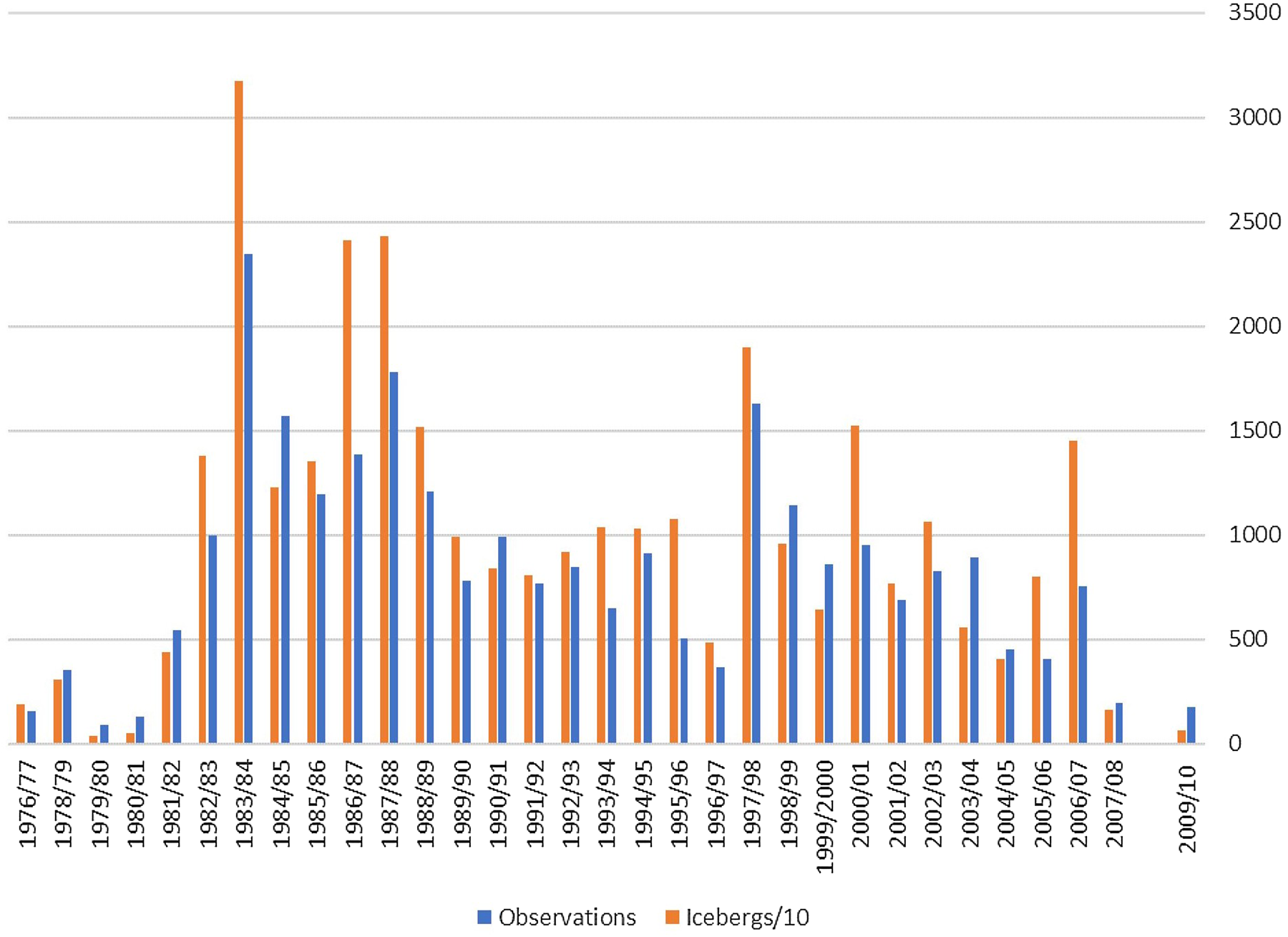
Figure 4 shows there are also large variations in proportions of different size classes, although only the two smallest size classes deviate from the regular pattern of decreasing numbers with increasing size. It should be noted in this connection that the seemingly increased number of smallest icebergs from 2003 onwards primarily reflects that the records for these years are mostly from the Antarctic Peninsula region, which has the larger proportion of smallest icebergs.
Percentages of icebergs in each size class.

The large variations shown by Figures 3 and 4 can arise from annual variations in iceberg production or from variations in time and space in the ship tracks. A first approach to evaluate this is to examine known variability in the ice discharge from the continent. The surface mass balance of Antarctic ice masses is everywhere positive, except for very small areas in the northern part of the Antarctic Peninsula and nearby islands, and very small blue-ice localities. Most studies indicate that practically all mass is lost by iceberg calving (~45%) and by melting from the underside of the floating ice shelves (~55%) (Depoorter and others, Reference Depoorter2013; Rignot and others, Reference Rignot, Jacobs, Mouginot and Scheuchl2013). Ice fluxes from the ice sheet are generally determined from measured or estimated ice velocities and thicknesses around the perimeter of Antarctica. The total ice flux across the grounding line provides an estimate of the steady ice discharge to the ocean, whereas the ice flux across an outer circumference near the fronts provides a steady-state estimate of iceberg calving. The year-to-year variability however, can be large (Liu and others, Reference Liu2015).
Various studies over individual years or multiyear periods and extending back to the start of these iceberg observations have given similar numbers for annual discharge, of ~2000 Gt (Kotlyakov and others, Reference Kotlyakov, Losev and Loseva1978; Budd and Smith, Reference Budd and Smith1985; Orheim, Reference Orheim1985; Warrick and Oerlemans, Reference Warrick, Oerlemans, Houghton, Jenkins and Ephraums1990; Jacobs and others, Reference Jacobs, Hellmer, Doake, Jenkins and Frolich1992). Recent numbers agree within 5–10% depending on the time period and data used (Depoorter and others, Reference Depoorter2013; Rignot and others, Reference Rignot, Jacobs, Mouginot and Scheuchl2013, Reference Rignot2019; Gardner and others, Reference Gardner2018). These differences are small compared with the recorded variations in time and space in the iceberg observations. However, the ice discharges computed from considerations of velocities and ice thicknesses are not the same as the calving rate. Icebergs of a wide range of sizes break off from the whole perimeter of Antarctica. Possibly the frequent smaller calvings, with sizes up to ~1 km, are stochastic independent events, however, we know this is not the case for giant icebergs. It is therefore particularly important to evaluate whether calvings of the largest icebergs cause spikes in the data, which could invalidate assumptions behind combining the annual records. Such spikes could, for example, occur along the trail of giant icebergs undergoing fracturing.
The calvings of the largest giant icebergs (>500 km2) are episodic on timescales of 10–100 a (MacAyeal and others, Reference MacAyeal2008) and they mostly originate from the few largest ice shelves. Ten calvings of icebergs >5 000 km2 surface area occurred during the years covered by the ship observations, and in the years of these extreme events the mass of Antarctic icebergs produced far exceeded the annual accumulation. Four of these icebergs were subsequently identified in ship observations, but without associated large increases in seasonal iceberg densities. Similarly, the yearly variations in calvings of icebergs with long axis >18.5 km registered in the NIC/BYU satellite database (Ballantyne and Long, Reference Ballantyne and Long2002; Budge and Long, Reference Budge and Long2018) are not directly reflected in the ship observations. The present database contains altogether 6436 icebergs >1 km in length, of which 93 were recorded as >10 km. Three of those in the NIC/BYU database were identified by onboard observers, but it is generally not possible to identify the source for most of the icebergs >1 km. When observed, they may still have approximately their original calved-off dimensions, or they may be remnants from the disintegration of yet larger icebergs. There are 92 one-time observations in the database of >100 icebergs in the open sea. Most likely these are associated with recent break-up of very large icebergs, but these observations are spread over 16 years, and do not significantly affect annual averages. We therefore conclude that even though some variations in iceberg density may be related to calving of giant icebergs, this does not explain the main variability in the data. Section 3.2.3 shows instead how the year-to-year iceberg observation variations are mostly explained by differences in the regions traversed by the ships. The record of giant iceberg calvings is described further in Table S8 and associated text.
3.2.3. Reality check on the year-to-year variations
To have confidence in the data it seems prudent to scrutinize them to see whether the large year-to-year differences can be ascribed to variations in ship tracks. Figures 3 and 4 and Table S3 show large variations in the average number of icebergs per observation and across size distributions between the years. However, some of these records are from a few cruises only, and with small numbers of icebergs observed. For a reality-check it is most critical to look at the records with many observations. Table S9 shows the results from all seasons in which more than 10 000 icebergs were observed. Examining the records for the seasons which deviate most from the mean in terms of either density of icebergs or size distributions shows that the sum of ship locations in each case also deviates from the average. The differences in iceberg statistics can thus mainly be accounted for by geographic differences between the cruises. Overall, the time of observation seems less important. This can be illustrated by sorting icebergs by month and by season, as shown in Figure 5 and Table S10.
Monthly and seasonal variations in percentages for each size class.

Looking at the variations during the year, the immediate impression is that the differences in iceberg size distribution are small, and that the differences in density are the opposite from what might be expected. The number of icebergs per observation is lowest in winter, June to September, when the ocean is coldest and melting of icebergs is lowest, and thus the highest numbers of icebergs could be expected if the iceberg production was steady throughout the year. Inspection of the records shows that the main reason for the low densities is, again, one of location. The extensive sea ice in winter forces the ship tracks much further north than in summer, thus there are very few overlaps in location for different seasons in the southernmost parts of the SO. The differences in location are also the main cause for the apparent paradox that the ‘winter’ observations show no significant difference in size frequency from the summer observations (December to March). In reality, the grid boxes with many observations over different parts of the year clearly show a decrease in iceberg frequencies and sizes through the summer period, in the same manner as shown by Jacka and Giles (Reference Jacka and Giles2007).
3.2.4. Are the observed iceberg numbers reasonable in relation to other knowledge on Antarctic iceberg production and distribution?
Whether the observed iceberg numbers seem reasonable can be evaluated by comparison with other databases of (a) ship observations and (b) satellite observations. As indicated in the introduction, the collection of systematic iceberg information was triggered by the observation that published ship records of Antarctic icebergs prior to 1980 seemed to be based on selective recordings. Four sets of iceberg data from coastal waters off East Antarctica published by Russian authors and which covered many seasons and ships totalled only 1663 icebergs. This was much less than those registered during either of two Norwegian Antarctic cruises (Orheim, Reference Orheim1980), and regional variations could not explain such large differences. Instead, the explanation for the differences between the Norwegian and Russian numbers seems to be that the latter recordings were episodic, focused on large or extraordinary icebergs.
There is now a much larger iceberg database available from Russian sources. Romanov and others (Reference Romanov, Romanova and Romanov2017) and Romanov and Romanova (Reference Romanov and Romanova2018) have presented compilations of records of ~70 000 iceberg observations from various Russian ship sources dating back to 1947. The core of the data derives from the research vessels of the Arctic and Antarctic Research Institute (AARI), but there are also substantial datasets from Russian whalers. Their dataset also incorporates those parts of the present database that were collected by Russian vessels, as well as part of the Australian dataset. In general, the Russian iceberg information, including the distribution patterns, agrees closely with that shown by the present database. However, the iceberg density given by Romanov and others (Reference Romanov, Romanova and Romanov2017) is less than half the present dataset (0.0033/0.0077 icebergs km−2). The difference could result from Russian vessels often recording icebergs only seen by radar, and perhaps also because personnel on whaling vessels chose not to record icebergs during busy whaling periods.
With regards to (b), satellite observations, it is shown above that the annual variations given in the present database do not correlate with satellite records of giant icebergs with long axis >18.5 km. Far more relevant for comparison, however, is the Altiberg database (Tournadre and others, Reference Tournadre, Bouhier, Girard-Ardhuin and Rémy2015), which uses satellite altimetry for regular mapping of icebergs of area 0.1– 10 000 km2. It contains monthly estimates of iceberg area and volume over 100 km × 100 km grid cells for the 1992–2014 period. It is thus a comprehensive satellite database that covers the two largest size classes of the ship records. However, there is considerable uncertainty in the size determination for the smaller icebergs. The distribution patterns given in the Altiberg database show high accordance with the distribution given in the present database, especially comparing Figures 9a, b of Tournadre and others (Reference Tournadre, Bouhier, Girard-Ardhuin and Rémy2015) with Figure 2 above. Where they overlap geographically, the satellite record therefore supports the results from the ship-based observations. However, the satellite record does not include ocean with sea-ice cover. It therefore provides limited data for the waters near the continent, where many icebergs are observed. For the same reason the satellite record has a large seasonal variation in iceberg quantities, with low numbers in winter when only the northern parts of the SO are observed. The satellite data are fundamental for systematic detection of larger icebergs, which is critical for ice mass and discharge considerations and for studies of iceberg movement. However, the sum of the smaller icebergs is important for calculations of impact on ocean water masses, and all sizes need to be included to understand the processes of iceberg dissolution. The databases are therefore complementary and a combination of databases should be considered for several purposes.
In summary, examination of the data and comparisons with other records of iceberg distribution supports the conclusion that the database reliably represents the iceberg distribution around Antarctica. Although episodic calvings of giant icebergs must cause spikes in iceberg densities, the main reason for the variations in the observed annual iceberg frequencies is differences in ship tracks. Combining multiyear observations thus forms a good foundation for determining average iceberg concentrations for different parts of the SO.
4. Analysis and results
Except where indicated the following analyses are based on the NPI component of the joint databases.
4.1. Iceberg distribution around Antarctica
Iceberg concentrations vary considerably around the Antarctic continent, and detailed examination of Figure 2 together with the iceberg densities in each gridbox reveals several notable features.
4.1.1. The coastal waters
Iceberg concentrations are high in most of the waters within ~200 km of the continent, indicating high incidences of iceberg production. Icebergs may also be concentrated by currents and by grounding. Moving clockwise around the continent from 0°E, we see that the iceberg densities are relatively high around most of East Antarctica, with lower concentrations near the coast only from 15–35°E and 110–150°E. Here, as elsewhere, north-flowing currents may remove icebergs from the coastal currents in exit zones, described below. The iceberg concentration in the southern part of the Ross Sea is very low, as a result of low calving rates from the Ross Ice Shelf, which infrequently produces mostly giant icebergs. Much higher concentrations are seen in the Amundsen and Bellingshausen Seas and along the western side of the Antarctic Peninsula. The north-eastern part of the Antarctic Peninsula and the south-eastern part of the Weddell Sea also exhibit high iceberg concentrations. Here the counter-clockwise coastal current around East Antarctica brings in additional icebergs.
We can compare this iceberg distribution with knowledge of iceberg production from other sources. First, regarding the largest or giant icebergs, the NIC/BYU satellite database shows that over the past four decades, 113 of these originated from their sector A (0–90°W), 100 from sector B (90–180°W) and 52 from sector C (90–180°E), while only 27 calved from the ice shelves in sector D (0–90°E). These calving frequencies are not mirrored in our observed iceberg concentrations, especially in sector D. That does not imply a contradiction however, given that giant icebergs are so infrequent. More relevant data are provided by Liu and others (Reference Liu2015), who give a comprehensive analysis of calving rates around Antarctica for the 2005–2011 period based on Envisat Synthetic Aperture data and visual interpretations. They concluded that the highest calving rate was from ice shelves facing the Amundsen Sea, which agrees well with the ship-borne observations. However, their Figure 1 gives low calving rates for the ice shelves from 30°W clockwise to 110°E, which does not accord with our high iceberg frequencies observed along most of this coast. One explanation for their low count of observed calving rates from this sector may be undetected calvings of smaller icebergs, perhaps in combination with high numbers of grounded icebergs observed multiple times from ships. This issue is discussed further in Section 4.4.
4.1.2. Iceberg exit zones
In general, icebergs follow the counter-clockwise near-coastal current until reaching four main exit zones (Fig. 6) where they are transported northward into the clockwise (towards the east) Antarctic Circumpolar Current (ACC). A common element of all exit zones is that the icebergs of high longevity may drift eastwards for many months in the ACC before disintegrating.
Approximate boundaries of the four main zones of iceberg export from the Antarctic continent, characterised by relatively high concentrations of icebergs. The land margins of Ross, Amundsen, Bellingshausen and Weddell Seas are shown by R, A, B and W. AP, Antarctic Peninsula; PIB, Pine Island Bay.

Exit zone 1 starts from ~85° to 120°E and extends northwards for >500 km. This is the smallest of the exit zones, indicating that many icebergs originating in East Antarctica drift westwards in the coastal current rather than exiting northwards. This zone has been described and analysed by Jacka and Giles (Reference Jacka and Giles2007).
Exit zone 2 extends westwards from south-western sections of the Antarctic Peninsula and the Bellingshausen and Amundsen Seas, from ~90° to ~140°W. Unfortunately, many grid boxes in this region lack observations (white in Fig. 6), which means that the boundary of zone 2 is in some places poorly defined, as indicated by dashed curves. The zone shows especially high iceberg concentrations north of the Amundsen Sea. Figure 1 shows that the number of observations in this area is low, so a few exceptional observations might explain the high densities. However, inspecting the individual observations in exit zone 2 shows many independent observations of large iceberg concentrations in different years, indicating that the high concentration is a real multiyear feature. This is most likely caused by high iceberg calving rates in the Pine Island Bay area, and possibly also high iceberg production rates from other calving glaciers in this sector of West Antarctica. It thus reflects the dynamic nature of the glaciers in this region, and strong north and west-trending currents. It is noticeable that the icebergs that calve in this sector mostly drift counter-clockwise, then north, rather than into the Ross Sea.
The third and largest exit zone extends more than 2000 km north-eastwards from the northern tip of the Antarctic Peninsula at ~60–65°S and 55°W. These icebergs must derive both from calvings on the eastern side of the Antarctic Peninsula and from icebergs that have drifted with the coastal current into the southern Weddell Sea and then northwards. After arriving at the northern tip of the Antarctic Peninsula these icebergs drift east-northeast in the ACC and persist in high concentrations to 0°E, 55°S.
Exit zone 4 reflects two sets of offshore currents. From ~15° to 30°W zone 4a extends westwards and north-westwards to give high concentrations in east-central Weddell Sea. As these icebergs continue to drift northwards, they merge into exit zone 3. From ~0° to 15° W the zone extends northwards, and may merge into exit zone 3, but also branches eastwards extending to ~20°E, 58°S. These two main drift patterns are also shown by transponder-tracked icebergs (Figs. 2c, e of Schodlok and others, Reference Schodlok, Hellmer, Rohardt and Fahrbach2006).
Figure 7 shows concentrations of observations of zero icebergs, and the high density of these in the southern and western Ross Sea is clear. This is also clear at the Antarctic Divergence, the upwelling zone at the southern front of the ACC, and a ship continuing northwards from there will usually encounter more icebergs.
Concentration of observations of zero icebergs. For each 1° × 5° box, this is defined as the number of observations recording no icebergs seen, divided by the total number of observations within that box. Smoothing has been applied to all the data. Boxes are filled white where there are no observations.

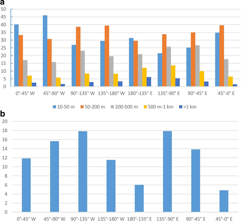
Figure 8 gives a broad overview of the iceberg distribution in sectors of the SO. By far the largest number of observations, and of icebergs, is from the sectors that include the Antarctic Peninsula. This region of many research stations exhibits a high density of small icebergs, to be expected since here there are relatively many glaciers calving directly into the ocean rather than forming ice shelves. The highest iceberg concentration is found in the adjoining sector to the west, with >17 icebergs/observation, while the 135–180°E sector has the lowest iceberg concentration, suggesting lower iceberg production in parts of this region. The Totten Glacier which forms the Totten Ice Shelf at 116°E drains much of the East Antarctic ice sheet to the west of 135°E, while the glaciers and ice shelves flowing east to the Ross Sea subtract from ice available to flow north in this sector. Unfortunately, this part of the Antarctic coastline has few stations, and sea-ice conditions often prohibit ship activity. Thus, iceberg statistics are not as robust as elsewhere. (Further information on iceberg distribution in the sectors is provided in Table S11.)
(a) Percentages for each size class in 45° longitude sectors around Antarctica. For each sector the data cover all observation latitudes. (b) Icebergs/observation for the same sectors.
4.2. Total number of icebergs in the Southern Ocean
The average concentrations and total numbers of icebergs for all parts of the SO may be calculated by combining all observations from each locality. As shown earlier there are large seasonal variations that become masked. The dissolution rate of icebergs within the sea-ice zone and in winter is low, and sometimes near zero. Once in open water, however, the majority of icebergs <1000 m disintegrate within a few months. A ship travelling south in the early part of the summer will thus encounter more icebergs in the open sea than on a repeat voyage later in the season. However, for most regions of the SO the data coverage is not sufficient to make robust calculations for different months. Given that most observations are from the summer, the following numbers can be seen as averages for that season.
In the following, the total number of icebergs, T, is calculated using the mean iceberg concentration in the individual grid boxes, defined as the total number of icebergs observed in the box divided by the number of observations. For a given region under consideration, the total, T, will then be the sum of icebergs across the latitude intervals φi to φj following Eqn (2):

where Fφ is the observed average iceberg frequency for the n o grid boxes with observations at the given latitude band, nφ is the number of grid boxes at that latitude, Aφ is the area of the grid boxes for this latitude interval (areas available in Table S7), and 1550 km2 is the area of an observation of 22.2 km radius.
Except for the northernmost waters, the few boxes that do not contain data have thus been assumed to have the same iceberg frequencies as the average frequency for the latitude interval in the zone under consideration. Using this approach means each gridbox is treated with equal weight, independent of the number of observations gathered in this box. A different approach might be to give each observation the same weight such that grid boxes with most observations have most influence. Because there are large differences in observation density, the results from the first approach are considered more likely to reflect reality. However, the second method would not result in large differences in derived numbers. Table 4 gives further details of the calculations, including the special treatment of the northernmost boxes.
Number of icebergs in assigned zones, each defined by logged observations within set 1° × 5° boxes. ‘S and N of 60°S’ refers to the remaining grid boxes in the SO not within the first five regions. ‘N of AC’ means north of the Antarctic Convergence, i.e. north of the SO boundary.

The iceberg concentrations vary from ~0.01 iceberg km−2 in the coastal waters and exit zones, to ~0.001 iceberg km−2 in the remainder of the SO. Near the coast, the average iceberg density is 0.0098 iceberg km−2, but with large variations. Some regions have four times higher iceberg frequencies, but there are also regions of zero or very few icebergs. The total area of the coastal zone is ~4.19 × 10⁶ km2, and the total number of icebergs there is ~41 000.
Away from the coast, the iceberg densities continue to show large regional variations related to the exit zones described in Section 4.1.2. Exit zone 1 covers an area of ~0.8 × 10⁶ km2, has an iceberg density of 0.0073 km−2 and contains 6000 icebergs. Exit zone 2 has an area of ~1.7 × 10⁶ km2 with 0.0093 iceberg km−2, for a total of 15 000 icebergs. The ~500 km wide exit zone 3 shows particularly high iceberg frequencies. It covers an area of ~3.2 × 10⁶ km2 with an average iceberg density of 0.0097 iceberg km−2, for a total of 32 000 icebergs. This offshore zone is the only one with the same high iceberg frequencies as the coastal zone. The fourth zone, which includes much of the Weddell Sea and covers ~1.7 × 10⁶ km2, has an iceberg density of 0.0069 iceberg km−2 and contains 11 000 icebergs.
Outside these zones the iceberg densities are an order of magnitude lower, apart from a few pockets of relatively high density mostly next to the high-density zones described above. The iceberg total for the whole remainder of the SO is 23 000. The number of icebergs at low latitudes is possibly exaggerated because of under-reporting of zero icebergs, as discussed earlier. No large errors likely arise from this, as the numbers are small compared with the iceberg numbers in the denser areas.
In summary, the total number of icebergs in the SO in the summer is ~129 000 icebergs, with ~130 000 altogether in the Southern Hemisphere oceans (Table 4). This is lower than the number given by Orheim (Reference Orheim1985) based on a much smaller set of iceberg observations, but very close to the result of Romanov and others (Reference Romanov, Romanova and Romanov2017). They give the instantaneous total number of icebergs in the SO as 132 269 (sic). The fact that the numbers are so close is surprising in view of their reported much lower average iceberg density, discussed earlier.
In the above calculations for the coastal zone and for the SO south of 60°S, the iceberg concentrations in the relatively few boxes without data are taken as equal to those in the data boxes at the same latitude. In the SO north of 60°S, only 104 of 326 grid boxes contain observations. Ships traversing these latitudes often logged no data. For these calculations boxes without observations are taken to have zero icebergs. The 62 boxes with icebergs north of the SO boundary are primarily in two areas; the largest stretches north-eastwards from exit zone 3 to 45°S, 5°W–15°E. The second, much smaller, extends from exit zone 1 north-eastwards to 49°S, 130°E.
4.3. Different drift patterns of small and large icebergs
Icebergs drift under the influence of several forces. The ocean current integrated over the draught of the iceberg is the most important, but icebergs are also affected by the Coriolis effect, by sea-ice forces when sea ice is present (Lichey and Hellmer, Reference Lichey and Hellmer2001) and by a tilt force from different centres of buoyancy/centres of gravity (Engelhardt and Engelhardt, Reference Engelhardt and Engelhardt2017). In general, the iceberg distribution shows good correspondence with the ocean circulation, but within this broad picture the different sized icebergs show differences in drift patterns, with the larger icebergs veering more to the left of the current. This accords with the model of Wagner and others (Reference Wagner, Dell and Eisenman2017) showing that the drift of small icebergs is more affected by the balance of wind and ocean currents than for large icebergs. The Coriolis effect becomes more important as iceberg mass increases, while wind and current forces act on the surface areas. This can be illustrated by looking at the proportion of the largest icebergs that either drift along the coast or enter exit zone 4, which extends west from 0°W. Here the counter-clockwise current that follows the coastline veers sharply to the left (south) at Cape Norvegia (10°W). In the coastal zone from 0–40°E the largest icebergs make up 2.7% of the total, while in the coastal zone from 0–40°W the proportion is 5.0%, and in exit zone 4 the proportion is only 1.0%. The corresponding numbers for the smallest size icebergs are 22.4, 21.8 and 33.8%. In other words, a much larger proportion of the largest icebergs than of the smaller icebergs veer to the left and follow the coastline southwards into the Weddell Sea. In general, the larger icebergs tend to ‘hug’ the continent, drifting in the counter-clockwise current. Similarly, the larger icebergs show a tendency to take a more northerly course than the smallest after exiting from the northern end of the Antarctic Peninsula.
Comparing the tracks of giant icebergs from 1999 to 2010 in Budge and Long (Reference Budge and Long2018) with the iceberg concentrations in this database (Fig. 2) also demonstrates that the giant icebergs take a markedly more northerly route than small icebergs. It would thus be misleading to use the observed tracks and distribution of the very large icebergs as a tool for predicting where the smaller icebergs can be expected. The drift of giant icebergs has been simulated by Rackow and others (Reference Rackow2017). Their computed tracks seem to be further north than indicated by satellite observations and would deviate even more for the smaller icebergs discussed here. However, England and others (Reference England, Wagner and Eisenman2020) and Huth and others (Reference Huth, Adcroft and Sergienko2022) show that iceberg break-up from buoyancy forces result in shortened ‘life spans’ for large icebergs and thus closer agreement with observations.
4.4. Estimate of annual iceberg calving rates
The iceberg distribution in coastal waters reflects the combination of local calving and advection of icebergs from adjoining seas. At the time of calving, the dimensions of icebergs from an ice shelf differ from those of icebergs calved from a tidewater or grounded glacier. The latter produces relatively small icebergs seldom exceeding 200 m in any dimension. Most Antarctic icebergs with dimensions >200 m, size class 3 or larger in this database, will have originated from ice shelves. Bindschadler and others (Reference Bindschadler and Choi2011) estimated the perimeter of Antarctica to be 53 610 km, 2/3 of which is in the form of ice shelves. The ice shelves produce the large icebergs that can be individually detected from satellites, and from 1979 onwards all giant icebergs >10 km are recorded, as described above. Liu and others (Reference Liu2015) have additionally, for the 2005–2011 period, recorded ~100 a–1 iceberg calving events >1 km2 from ice shelves exceeding 10 km2.
There are relatively little data available on smaller iceberg calvings from the ice shelves. The ship records from the coastal waters reduce this information gap and indicate that smaller calvings may have gone undetected to the extent that they affect mass-balance conclusions. To investigate this further we can examine the iceberg distribution in the coastal waters of East Antarctica, from 0° to 170°E longitude, a coastline almost completely consisting of ice shelves and shorter sections of pinning ice rises. This part of the Antarctic coast has the most regular geometry, being almost circular. The ocean current runs counter-clockwise along the coast, which means that observed icebergs have either advected from the east, or have calved locally. It is then possible to use the combination of iceberg frequencies and size class variations to derive information on calving activities along the coast.
Appendix A Table 5 and Figure 9 show the iceberg distributions along the ~200 km wide coastal zone of East Antarctica. The 51 000 observed icebergs have been grouped into the smallest (class 1 + 2 for NPI and ANARE) and largest (class 5 for the 5–class NPI, classes 5–7 for the 7–class ANARE) icebergs. The 5–7 class ANARE data are >800 m, while the NPI class 5 is >1 km. The ANARE data add substantially to NPI data for the longitude interval 60–120° E and are therefore included, even though the size class boundaries differ. In this coastal region the two smallest ice classes make up 44%; the largest makes up 4.2%, and the number of icebergs per observation is 14.4. It thus contains a higher proportion of the larger icebergs, and more altogether, compared with the dataset as a whole (72.4%, 2.5% and 12.0 icebergs per observation).
Iceberg densities and percentages of smallest and largest icebergs for 5° longitude sectors of the coastal zone of East Antarctica. Note there are no data for the 150–155°E sector.
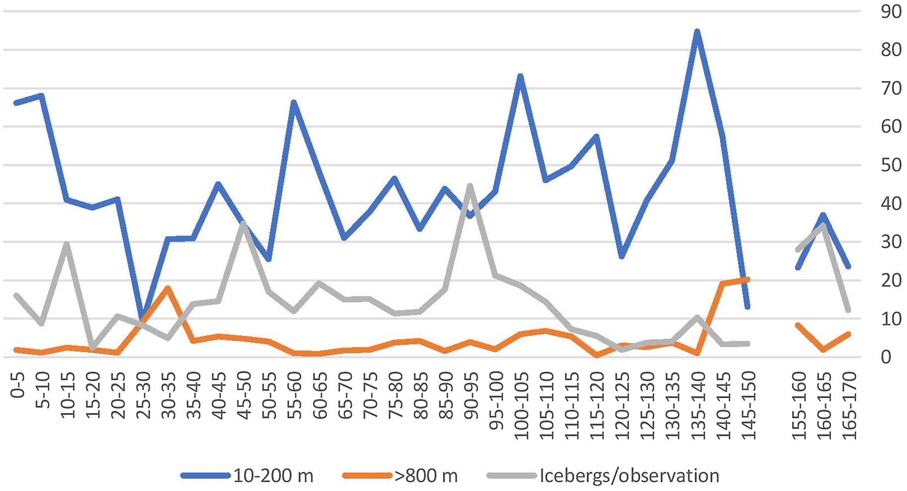
With the caveat that the years covered by the data are not always identical, and using caution for areas with relatively few observations, it is nevertheless clear that there are real differences across the longitude bands. These must mostly be related to local calving events. If advection of icebergs from the east were the main source of the differences, a systematic reduction in size and possibly an increase in concentration would be expected following the coastal current to the west. Such systematic changes in size and concentration are not shown in Appendix A. Instead, Figure 9 shows several abrupt changes to the contrary, e.g. decreased concentration from 145° to 130°E and an increase in largest icebergs from 115° to 105°E and 60° to 45°E. These can only be ascribed to high calving rates. The changes in dimension or density cannot be ascribed to advection into or from adjoining waters to the north. The only major iceberg drift in this respect is for those leaving exit zone 1, from ~85–120°E, described above.
The observations from Jacka and Giles (Reference Jacka and Giles2007) can be used to get a perspective on the numbers in Appendix A. They indicate a drift speed of 5 km d–1 and dissolution rate of 0.03 m d–1 in these cold waters. The travel distance at 5° longitude along 68°S is 208 km. It will thus take 6 weeks to cross one 5° longitude band, and during this period the iceberg will have lost ~15 m from each side (and base). This loss will significantly affect the numbers of the smallest icebergs, but not the larger ice classes.
Figure 9 and Appendix A indicate high calving rates at 155–170°, 140–150°, 90–115°, 45–55°, 25–35° and 10–15°E. It is of interest to compare these results with Liu and others (Reference Liu2015), who have provided the most comprehensive analysis of iceberg calving rates around Antarctica. For the 2005–2011 period, they recorded 579 distinct iceberg calving events >1 km2 from the ice shelves >10 km2 in area and summarized a calving rate of 755 Gt a−1 for all of Antarctica. Their Figure 1 shows that of this, only 55 Gt a−1 came from the coast between 0° and 100°E, while 230 Gt a−1 came from the coast between 110° and 155°E. This is not in accord with the present data for the 0–100°E sector. Possible explanations for their low observed calving rates from this sector, representing a major part of East Antarctica, could be errors/uncertainties in this SCAR dataset, or either less calving than normal during the 2005–2011 period or undetected calvings. With a resolution of 1 km, any smaller icebergs breaking off from an ice front with an approximately fixed front position may not be detected.
5. Conclusions and perspectives
The strength of the SCAR International Iceberg Database is the large number of observations over many years using identical recording protocols for standard iceberg sizes, providing systematic coverage over most parts of the waters around Antarctica. The data are particularly useful because they include systematic observations of all the smaller icebergs, which are not covered by current satellite-based databases. We have demonstrated in this paper that the database provides insights on iceberg quantity, distribution and drift patterns over most of the SO, and on iceberg calving rates. The database should also be useful in studies concerning iceberg dissolution rates, ‘life expectancy’, contribution to ocean temperatures and salinities, and Antarctic ice-sheet mass balance. The release of these extensive iceberg data will therefore hopefully trigger further applications and, in combination with modern satellite data, more in-depth studies.
Supplementary material
The supplementary material for this article can be found at https://doi.org/10.1017/jog.2022.84.
Data
The SCAR International Iceberg Database presented in this paper can be accessed through the SCAR data depository and through Norwegian Polar Institute data records at https://doi.org/10.21334/npolar.2021.e4b9a604
Acknowledgements
The NPI and ANARE databases derive from 233 ship cruises involving 68 vessels from 20 different SCAR nations. Data have been collected by more than a thousand individual observers. With this database and publication, we extend our deep gratitude to the national Antarctic programs for accommodating this program on their ships, to the observers for their unfailing efforts, and to ship's officers for sharing knowledge and advice with those observers. We are also grateful to the various directors and program leaders of NPI, AAD and ACE CRC who have supported the compilation of these databases. Over the years, from when the program started until today, several persons have also contributed to the registration of data and to considerations of how they should be analysed. In this connection we give special thanks to Øyvind Finnekåsa, Bjørn O. Johannessen, Stein Tronstad and Jan-Gunnar Winther, all working at the time at the Norwegian Polar Institute, and Vin Morgan, Trevor Hamley and Neal Young, at the time at AAD. Comments from two anonymous reviewers significantly improved this paper. As we prepare for final submission of this paper, we have learnt of the death of WF (Bill) Budd. Bill was part of the initial SCAR meeting that endorsed the collection of these data and it was he who initiated the Australian contribution. We dedicate this paper to Bill Budd.
Author contributions
O.O. initiated the original data collection program and wrote the initial version of the text. B.G. and G.M. provided analyses and figures. J.J. co-ordinated the ANARE data collection throughout the collection period. All authors commented on and revised the text and approved the final article.
Financial support
This work has been financed by the Norwegian Polar Institute, Tromsø, Norway and in Australia by the Institute for Marine and Antarctic Studies, University of Tasmania, Hobart and Australian Antarctic Division, Kingston, Tasmania.
Appendix A
East Antarctic iceberg distributions
The distribution of smallest and largest icebergs in the East Antarctic coastal zone


 Open access