


1 Introduction
Many inferences in Political Science are based on quantitative models with multiplicative interaction terms (Brambor et al. Reference Brambor, Clark and Golder2006). Ten years ago, a code of best practice for interaction models has been suggested (Brambor et al. Reference Brambor, Clark and Golder2006). This paper has been cited more than 3600 timesFootnote 1 since then, a clear sign of the ubiquitous use of these models and of researchers’ interest in avoiding inferential errors. Models with quadratic terms are similarly widespread and can be understood as a specific type of interaction model (on the latter point see Brambor et al. Reference Brambor, Clark and Golder2006).
While the specification and interpretation of interaction effects of interest has improved greatly in the past ten years, control strategies for models with product terms—that is interaction and non-linear effects—have received little attention. Typical specifications follow the control strategies recommended for models without product terms and assume a linear, non-conditional effect of potential confounders on the outcome variable or latent underlying variables. But this strategy is not sufficient to prevent biased inference in models with product terms. Interaction terms in models can pick up the effects of un-modeled interaction and quadratic terms, and analogously, included quadratic terms can reflect omitted interaction and quadratic terms. This problem can occur even when included and omitted product terms do not share any constitutive terms.
In this article, we show that a control strategy that assumes a linear effect of potential confounders for constitutive terms in a product term is not able to prevent this type of bias. We describe the possible ways in which omitted product terms can bias conclusions about included product terms and what theoretical considerations researchers need to make when developing their control strategy. In addition, we suggest estimation strategies that deal with the issue of bias stemming from omitted product terms and show in Monte Carlo analyses that they prevent the misattribution of interactive and quadratic effects while at the same time minimizing the problems of efficiency loss and overfitting.
Papers on interaction models (Brambor et al. Reference Brambor, Clark and Golder2006; Berry et al. Reference Berry, DeMeritt and Esarey2015, e.g.) focus on models with one interaction and the correct specification, estimation, and interpretation of this interaction.Footnote 2 For simplicity, it is assumed that the interaction of interest is the only interaction in the model. The recommendation of Brambor et al. (Reference Brambor, Clark and Golder2006, 64) that “[a]nalysts should include interaction terms whenever they have conditional hypotheses” is sound advice in the context of this type of scenario. However, empirical data generating processes are more complex and it is likely that in many cases several non-linear or conditional relationships affect an outcome of interest. We show here exactly when and how ignoring other conditional and/or non-linear effects by including only the product term of interest in the model—as is common practice—can bias inferences about the product term of interest as well as other variables in the model. The correct specification of control terms in models with product terms is as important as the correct specification of the product terms of interest themselves.
Many researchers include control variables in a linear fashion when testing non-linear and interactive relationships. Of course, the reason for this could be a theoretically guided expectation that none of the control variables has a non-linear effect or is moderated by another variable. We suspect, however, that many researchers are not aware that, when modeling interactive or quadratic relationships, it is particularly important to consider for each control variable whether it could have a non-linear or conditional effect that could be picked up by product terms in the model. Supporting this, we discuss some examples in the appendix (Section 4) where researchers interested in conditional relationships include linear control variable specifications even when they are aware that these control variables may have non-linear or conditional effects themselves. It is, however, not our intention to single out the articles we describe. We suspect that the practice of not considering whether product terms are included as control variables may be necessary is widespread.
We have surveyed 40 recent papers in top journals and top subfield journals of Political Science that cite Brambor, Clark and Golder's seminal paper.Footnote 3 Table 1 displays summary statistics from this literature review. We find that of the 39 papers that included a product term, only ten (≈25 percent) are considered and included additional product terms amongst control variables as well. In the majority of articles, researchers seemed to assume that adding additive control variables is a sufficient control strategy for factors that could be possible confounders for an interaction term. Furthermore, for the 41 percent of papers that hypothesize multiple conditional effects, less than half include all of these product terms in their empirical model at the same time.
The use of product terms in political science research

One reason why many researchers do not address the problem could be that they are uncertain about an appropriate solution. A natural concern would be that including all potentially relevant interactions and squared terms in a model leads to overfitting and a severe loss of statistical efficiency. We suggest three estimators, the adaptive Lasso (Zou Reference Zou2006; Kenkel and Signorino Reference Kenkel and Signorino2013), KRLS (Hainmueller and Hazlett Reference Hainmueller and Hazlett2014), and BART (Chipman et al. Reference Chipman, George and McCulloch2010; Green and Kern Reference Green and Kern2012), that allow researchers to identify necessary interaction and non-linear effects as part of their control strategy. We analyze the performance of these estimators in Monte Carlo simulations on a wide array of situations. Our Monte Carlo experiments show that these techniques perform well for selecting product terms necessary to avoid bias without overfitting the model or creating unnecessary inefficiency. This is even the case when up to ten covariates, and all their product and quadratic terms, are included in a model. In addition, the estimators in most conditions do not perform substantively worse than a parametric specification based on the correct data generating process.
The paper proceeds as follows: First we demonstrate the issue of omitting product terms as part of the control strategy. Next we introduce solutions that can help researchers to ensure their inferences from interaction and quadratic terms are accurate and robust. Next, using Monte Carlo experiments, we confirm the potential for bias in a range of scenarios, for both continuous and binary-dependent variables, and the improved performance when using either one of our suggested solutions: the adaptive Lasso, KRLS, and BART. We also demonstrate that the adaptive Lasso is the best choice for an applied researcher on average, due to its better performance regarding false positives, greater computational speed, and more intuitive parametric form. Finally, we use a recent paper to illustrate how inferences drawn can change when relevant product terms are used in the control strategy.
2 The problem
2.1 Illustrating the problem
To illustrate the issue with omitting quadratic and interaction terms amongst the control variables, consider the following example: A country's economic inequality may increase the likelihood of a civil war breaking out.Footnote 4 This has been found in numerous studies considering inequality between ethnic groups and ethnic conflict (e.g.,Cederman et al. Reference Cederman, Weidmann and Bormann2015) as well as in the context of non-ethnic conflict (e.g., Bartusevičias Reference Bartusevičias2014). Additionally, it could be argued that in democratic states, conflict is less likely because they offer peaceful opportunities for action. This might lead a researcher to hypothesize that the effect of inequality is moderated by the regime type of the state: In a democracy, inequality may be less likely to trigger collective violence than in an autocracy as less wealthy citizens still have the opportunity to vote for parties that promise to improve their situation. When testing this interaction, and following the currently widespread control strategy for interaction models, a researcher would include countries’ GDP per capita in the model. After all, numerous previous studies have found a country's GDP to have a negative effect on civil war (e.g., Collier and Hoeffler Reference Collier and Hoeffler2004), and GDP is likely correlated with democracy and inequality.
As we show in this paper, the inference drawn about the effect of inequality conditional on the level of democracy in our hypothetical model will be biased if there is another variable that moderates the effect of inequality and is correlated with democracy. For example, it could also be the case that the effect of inequality is moderated by a country's wealth instead of or alongside its regime type. Koubi and Böhmelt (Reference Koubi and Böhmelt2014) argue that in richer countries, inequality causes greater grievance which in turn increases the likelihood of conflict.Footnote 5 If the interaction term between inequality and GDP is omitted, as is current practice, the interaction term between inequality and democracy will reflect the coefficient of the omitted interaction term in the data generating process if GDP is correlated with regime type. Importantly, including GDP as an additive control variable, as the usual strategy would suggest if GDP is suspected to be correlated with the regime type as well as the outcome variable, is not sufficient in order to prevent this bias.
The same logic also applies to squared terms as a specific form of interactions. For example, many researchers have been interested in an inverse u-shaped effect of the regime type on civil conflict (for an overview, see Vreeland Reference Vreeland2008). If a model testing this expectation included inequality as an additive control variable, the conclusion about the effect of the regime type could be biased if in the true model democracy moderates inequality and this interaction term is omitted. Similarly, if the regime type had an inverse u-shaped effect in the true model and a squared term is omitted, an interaction term between inequality and democracy will be biased if regime type and inequality are correlated.
These examples illustrate common issues with omitting product terms amongst the control variables, that much of the literature has ignored. However, omitting product terms can also introduce bias in more complex ways. The next section discusses when and how excluding product terms from one's control strategy introduces bias.
2.2 The problem of omitting product terms
Like omitting a variable that has a linear effect on an outcome variable causes bias to correlated variables included in a model, omitting product terms can cause bias to included terms, especially if they are specified by a product term. In this section, we give an overview over the circumstances under which this is the case. In the supplementary appendix, Sections 2 and 3, we show a detailed analytic derivation of the circumstances under which omitting product terms introduces bias.
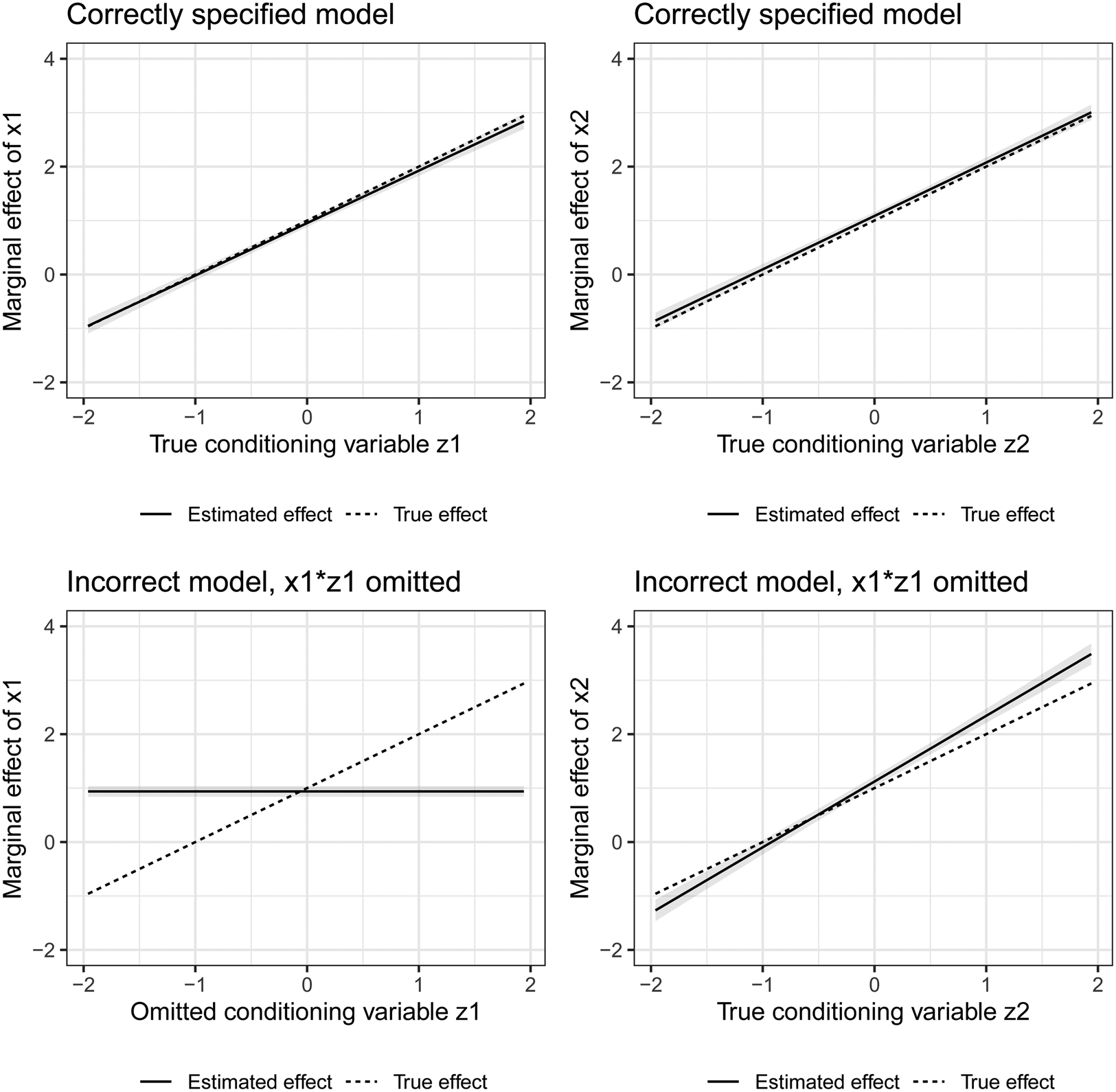
The most straightforward case of bias due to an omitted product term occurs when a researcher includes an interactive term between two variables but omits an interaction term that is relevant in the data generating process and that shares a constitutive term with the included interaction term. This bias will affect the coefficient of the included interaction term as well as the coefficients of its constitutive terms. For this bias to occur, it is sufficient for a false moderator, z 2, of a variable x to be correlated with the true, yet omitted, moderator of x, z 1. It is even sufficient for the excluded true moderator z 1 and the included false moderator z 2 to both be correlated with x. As illustrated in Figure 1, these biases occur even though the correct moderator of x, z 1, is included in the estimated model as an additive regressor alongside the interaction term between x and z 2.Footnote 6
Conclusions about moderating variables of x based on correct ($y = \beta _x x + \beta _{z_1} z_{1} + \beta _{x z_1} x z_{1} + \beta _{z_2} z_{2}$ ) and incorrect model specification ($y = \beta _x x + \beta _{z_1} z_{1} + \beta _{z_2} z_{2} + \beta _{x z_2} x z_{2}$
 ). z 1 and z 2 have a correlation of 0.5.

The logic also holds if both x z 1 and x z 2 are relevant in the data generating process or when a relevant squared term is omitted that shares a constitutive term with an included interaction—and vice versa.Footnote 7 An interaction term that is included in a regression can pick up the non-linear effects of the variables included in the interaction term, suggesting conditional effects even when they do not exist.Footnote 8 In addition, the problem also persists in a less intuitive case: an omitted product term—squared or interactive—can even bias an included product term if it does not share a constitutive term with it. As illustrated in Figure 2, an included interaction term x 1 z 1 will be biased by an omitted product term x 2 z 2 if x 1 and x 2 as well as z 1 and z 2 are correlated—or the other way around. Again, the same logic extends to quadratic terms being the included or excluded product term in this scenario.
Conclusions about moderating variables of x 1 and x 2 based on correct ($y = \beta _{x_1} x_{1} + \beta _{z_1} z_{1} + \beta _{x_1 z_1} x_{1} z_{1} + \beta _{x_2} x_{2} + \beta _{z_2} z_{2} + \beta _{x_2 z_2} x_{2} z_{2}$ ) and incorrect model specification ($y = \beta _{x_1} x_{1} + \beta _{z_1} z_{1} + \beta _{x2} x_{2} + \beta _{z_2} z_{2} + \beta _{x_2 z_2} x_{2} z_{2}$
 ). x 1 and x 2 have a correlation of 0.5 and z 1 and z 2 have a correlation of 0.5.
This form of bias requires researchers to think carefully about whether there are possible other non-linearities or interactions in the data generating process. While this is always important as any misspecification can cause bias amongst included variables, it is particularly important when product terms are of interest in a model as un-modeled product terms will be picked up by included product terms leading to an incorrect conclusion about interactive or non-linear effects of interest. Therefore, researchers that are interested in interaction effects need to consider whether there is another variable that could moderate one of the variables in their interaction term of interest. Similarly, they need to consider whether any of the variables in their interaction of interest could have a quadratic effect. Finally, researchers including an interaction term need to consider whether there could be an omitted interaction or squared term that—albeit not sharing a constitutive term with the included product term—has constitutive terms that are correlated with both constitutive terms of the included interaction. Analogous considerations need to be made when researchers are interested in quadratic relations.
3 The solution
Having demonstrated the possible ways in which omitted product terms can bias conclusions about included product terms and what theoretical considerations researchers need to make when developing their control strategy, we now turn to investigating the performance of possible solutions for the issue. While omitted product terms expose models to bias and will likely lead to incorrect inferences about non-linear and conditional effects, simply interacting all control variables with the variables in the interaction of interest, as well as with each other and squared terms for every variable in the model, leads to the inclusion of a large number of additional terms (also see Hainmueller and Hazlett Reference Hainmueller and Hazlett2014, on this point). This may be problematic, as previous research has identified that simply adding more terms to regression models does not automatically lead to a reduction in bias, and under certain conditions may even increase it (Clarke Reference Clarke2005, Reference Clarke2009). Moreover, the inclusion of more parameters to estimate will reduce the efficiency of the estimation. This problem is particularly severe in the case of binary choice models, such as Logit. Therefore, it is important to restrict the set of product terms to be included in an empirical model to the ones relevant for preventing bias. Researchers need to be able to select relevant product terms and omit irrelevant ones in a systematic way. We suggest penalized regression as an approach that allows researchers to do so.
We focus on three specific regularized regression methods: the adaptive Lasso, KRLS, and BART.Footnote 9
The first method is the adaptive Lasso, used in a similar manner as Kenkel and Signorino (Reference Kenkel and Signorino2013).Footnote 10 Importantly, the adaptive Lasso has the oracle property (Zou Reference Zou2006). That is, as the sample size increases, the adaptive Lasso performs as well as if we knew the “true” model in advance and the probability of the coefficient of an irrelevant variable being constrained to zero converges to one. Thus, if the potentially relevant product terms do not actually have an effect, Lasso will constrain them to zero and minimize the loss of efficiency incurred in an unpenalized model. As noted above, one of the two relevant conditions for bias is that the omitted interaction term has an effect on the outcome in the data generating process. The Lasso ensures that these terms are included which is effective to prevent bias. At the same time, the estimator sets parameters associated with variables that do not have an effect upon the dependent variable to zero thereby avoiding the loss of efficiency incurred by including them. The adaptive Lasso can be used to model continuous as well as binary outcomes.
The second solution is the use of KRLS (Hainmueller and Hazlett Reference Hainmueller and Hazlett2014). KRLS assumes a parametric model that allows for highly non-linear functions. However, instead of relying on linear-additive Taylor approximations, as our use of the adaptive Lasso does, KRLS defines the set of candidate functions through the superpositioning of Gaussian kernels. This model is able to approximate functions of x on y of almost any form, in a more flexible manner than the polynomial approximation used in our application of the adaptive Lasso. Similar to the adaptive Lasso, the specified model is fitted to the data and simultaneously regularized with a penalty term that is opposed to complex functional forms, which is chosen using generalized cross-validation. While the adaptive Lasso can be explicitly adapted to binary choice models, this is not the case for KRLS. However because KRLS is extremely flexible in estimating functional form, it is assumed to produce valid inference even for binary responsesFootnote 11, thus significantly expanding the range of possible applications.Footnote 12
The third solution is the use of BART. Most visibly popularized in Political Science by Green and Kern (Reference Green and Kern2012), BART is typically used to analyze treatment effect heterogeneity. Developed by Chipman et al. (Reference Chipman, George and McCulloch2010), BART consists of estimating an ensemble of regression/classification trees, which are summed over. This allows the researcher to estimate a smooth relationship between the outcome and independent variables, unlike single-tree models which fit piecewise-constant functions. Within the ensemble of trees, each tree can potentially capture some interactive or non-linear relationship between variables and the outcome, allowing the estimation of complicated functional forms. Finally, these inferences are regularized with the use of priors on the various hyperparameters, for example, placing greater weight on smaller trees (i.e., those with less complicated interactions), in order to prevent overfitting.
The trade off between these models is the common bias versus efficiency problem faced when choosing how parametric of a modeling approach to take. While the adaptive Lasso is known to be biased, due to setting parameters exactly to zero, it is as a result a more efficient estimator. The parametric form we use, ruling out more complicated functional forms, also leads to our use of the adaptive Lasso likely being more efficient than KRLS and BART. Furthermore, the adaptive Lasso should be more efficient than KRLS as this model makes explicit distributional assumptions about the dependent variable. Nevertheless, as it is hard to know the relative importance of these aspects a priori, we leave it to the Monte Carlo experiments to assess the relative strength and benefits of these models from this perspective.
It is also important to note that these solutions focus predominantly on dealing with continuous and binary outcomes. Nevertheless, there are solutions for researchers who deal with ordinal or multinomial outcomes. There exist Lasso implementations for ordered outcomes (Wurm et al. Reference Wurm, Rathouz and Hanlon2017) and for multinomial outcomes (Friedman et al. Reference Friedman, Hastie and Tibshirani2010). However, as equivalent implications for our alternative estimators do not exist, we focus our Monte Carlos only on the continuous and binary cases, to inform researchers on the relative strengths and weaknesses of competing estimators.Footnote 13
4 Monte Carlo analysis
Having discussed the analytical bias from the current practice of including interaction and squared terms without appropriate control variables, we now conduct a Monte Carlo study in order to characterize the problem under a wider range of scenarios. While the first impulse would be to examine bias and RMSE in parameters when researchers fail to include a relevant interaction or quadratic term, the results of doing so are easily derived analytically and find that failing to do so leads to bad inferences.Footnote 14
Instead we focus on how our ability to make inferences about conditional/non-linear relationships is impacted when we move beyond including one product term, to scenarios where we include many product terms. Furthermore, we explore scenarios where there is such uncertainty about the set of relevant product terms, that researchers would include all possible product terms from their included variables. In doing so, we will focus on the extent to which we generate false positives (i.e., find relationships for irrelevant product terms) and false negatives (i.e., fail to find the relevant relationships for product terms, due to attempting to include too many product terms). We focus on binary outcomes, instead of continuous outcomes estimated with OLS, as the standard estimators for binary outcomes, such as Logit, are particularly sensitive to misspecification and the inclusion of irrelevant variables.
Our data generating process is:

where a i, b i, and c i are jointly drawn from a multivariate normal distribution with mean zero and variance one, and covariance ρ.Footnote 15 εi is drawn from a logistic distribution with mean 0 and variance π2/3, and a binary variable y i is created that equals 1 when $y^\ast _{i} \gt 0$ and equals 0 otherwise.
For all experiments, we set the coefficients for the constitutive terms βa and βc to be equal to 0.5, and − 0.5 for βb. Values of the coefficients for the product terms βac and $\beta _{b^2}$ are set to 0.5, and to − 0.5 for βab. For each scenario, we compute 40 Monte Carlo iterations.
Our Monte Carlo experiments focus on how our ability to derive inferences about conditional and non-linear relationships are affected by the following two factors:
1. The covariance (ρ) between the independent variables (ρ ∈ {0.25, 0.5, 0.75})
2. The number of observations (n ∈ {500, 1000, 3000})
We compare the following estimators and specifications:
• KRLS
• Adaptive Lasso including all interaction and quadratic terms
• BART
• Logit including all interaction and quadratic terms (i.e., over-specified parametric model)
• Logit using the correct model specification (i.e., true model)
For each statistical model, we also include seven “irrelevant” variables (d to j), and all possible product terms in the parametric models, to assess the estimators’ sensitivity toward over-specification. These irrelevant variables have no impact upon the outcome y, but are also correlated with a, b, and c by the value of ρ in a given scenario.Footnote 16
To ensure comparability between the statistical estimators, we focus on the second difference in predicted values from the estimators. The second difference is how the effect of moving a variable, x, from a low (x l) to a high value (x h) changes dependent upon another variable, z (see also Berry et al. Reference Berry, DeMeritt and Esarey2015).Footnote 17 The second difference directly measures interactive and non-linear hypotheses, as interactive and non-linear hypotheses are about how the effect of a variable changes, given the value of an other variable or itself. More formally, the second difference is:

where x is the variable whose effect is moderated by z, and f is the function that translates data and estimated coefficients into predicted values of the outcome variable.Footnote 18 For the adaptive Lasso and KRLS, we supplement this with bootstrap aggregation (bagging), based on 200 bootstrap samples per iteration, to enable more stable estimates and generate confidence intervals. For BART, we calculate uncertainty estimates using the draws from the posterior distribution.
While these settings apply generally, we do encounter a problem with KRLS when extending our Monte Carlo experiments to including 3000 observations. With this number of observations, the implementation of KRLS in R by Hainmueller and Hazlett (Reference Hainmueller and Hazlett2014) is extremely computationally demanding. To remedy this, we instead use bigKRLS created by Mohanty and Shaffer (Reference Mohanty and Shaffer2016) for such situations. While this implementation of KRLS offers considerable speed improvements, it is still not sufficiently fast within our Monte Carlo setup to let us calculate bootstrapped confidence intervals as we have done previously.Footnote 19 Therefore, we only report estimated second differences, without bootstrapped confidence intervals for the KRLS estimator when the number of observations is 3000.
4.1 Varying the covariance between independent variables
Figure 3 displays the second differences from the adaptive Lasso, KRLS, BART, the over-specified parametric, and the correctly specified models for the relevant independent variables. In this figure, the effects of a conditional upon b and c (and vice versa) are correctly picked up by the adaptive Lasso and KRLS. However, the magnitude of these effects estimated by the adaptive Lasso and KRLS is smaller, being approximately 55–65 percent of the size of the effects in the true specification when the correlation is 0.75. While the magnitude of the second difference is closer approximated by the over-specified parametric logit model, the uncertainty associated with this estimate grows considerably larger than the other estimators, the higher the level of correlation between the variables. The second differences estimated when using BART however are far more sensitive to the level of correlation between regressors. While conditional effects are correctly identified when the level of correlation is low (0.25), it performs poorly when the level of correlation is high (0.75). In this case, all of the estimate second differences are very close to zero.
Estimated second differences for relevant variables. The confidence/credible intervals are displayed in gray, while the mean of the second differences for all 240 simulations is displayed in white. Columns indicate the statistical model, and rows indicate the level of correlation between the independent variables.

Turning to the uncertainty estimates, the estimated 95 percent confidence intervals for KRLS and the adaptive Lasso perform well but do tend to be conservative, particularly in cases with high correlation between covariates. While the confidence intervals for the relevant variables from the adaptive Lasso include zero approximately 7 percent of the time when the correlation between variables is 0.25, this rises to approximately 90 percent of the time when the correlation between variables is 0.75. For KRLS, at a correlation of 0.25, approximately 12.5 percent of confidence intervals include zero, while at a correlation of 0.75 approximately 70 percent of confidence intervals include zero. In the case of BART as the second differences are close to zero when the correlation is high, the credible intervals unsurprisingly include zero.
Figure 4 displays the median second difference from the models displayed previously. The results support the general pattern found previously, that the KRLS and adaptive Lasso are more conservative estimators than the over-specified parametric model. However, BART is considerably more conservative, particularly as the level of correlation between independent variables increases. While the second difference estimates become smaller relative to the true estimates for all approaches as the correlation increases, they are very close to zero for BART at correlations of 0.5 and higher. Nevertheless, they still remain in the correct direction, and in the case of the Lasso and KRLS are not significantly different from the true second differences.
The median estimated second differences for relevant variables. Columns indicate the level of correlation between the independent variables, while color and shape indicate the statistical model used.

Having examined the performance of the estimators for the relevant second differences (i.e., where there exists a true effect), we now turn to exploring how the estimators perform with regards to irrelevant variables (i.e., variables that do not have a conditional or non-linear effect upon the outcome). As we can see in Figure 5, the estimators work well on average. The mean estimated second differences are close to zero, and the 95 percent confidence intervals all include zero. Therefore, even in the case of a logit model with many highly correlated product terms, the risk of false positives remains low.
Estimated second differences for irrelevant product terms. Each white point corresponds to the mean second difference estimated for every irrelevant combination of variables. The confidence/credible intervals are displayed in gray. Columns indicate the statistical model, and rows indicate the number of observations.

Figure 6 explores this issue in greater depth, displaying the median estimated second difference for all of the possible conditional effects including irrelevant variables for each model. From these results, we can see the adaptive Lasso and BART perform particularly well in terms of avoiding false positives. While their performance becomes slightly worse, the higher the level of correlation between the variables, their average second difference is consistently close, if not equal to, zero. While KRLS and the over-specified parametric Logit model do not perform too badly substantively, they are consistently outperformed by the adaptive Lasso and BART with the Lasso and BART having smaller (i.e., more accurate) second differences for 95 and 100 percent of estimates compared to the over-specified parametric model and KRLS, respectively.
The median estimated second differences for irrelevant product terms by statistical model used. Each point corresponds to the median second difference estimated for every combination of variables that have no conditional effect. Columns indicate the level of correlation between the independent variables, while color and shape indicate the statistical model used.

4.2 Varying the number of observations
We now turn to examining how our ability to identify conditional and non-linear relationships is affected by the number of observations available. Therefore, we vary the number of observations in our Monte Carlo experiments, setting them to 500, 1000, and 3000.
Figure 7 displays the second differences from the various models analyzed. As would be expected, the level of uncertainty associated with the second differences, in terms of the 95 percent confidence intervals, is higher, the lower the number of observations. However, most estimators manage to return on average the correct estimates for the relevant second differences, even in the case of 500 observations. This is in spite of the fact that there are many other irrelevant product terms included in the Lasso, and other non-linearities and conditionalities allowed by KRLS. The one exception is the performance of BART at a low level of observations. In this case, the estimator, as highlighted previously, is particularly conservative, with all second differences being estimated close to zero.
Estimated second differences for relevant variables. The confidence/credible intervals are displayed in gray, while the mean of the second differences for all 240 simulations is displayed in white. Columns indicate the statistical model used, and rows indicate the number of observations.

Figure 8 displays the median second difference from the models displayed previously. The results suggest that while the adaptive Lasso tends to be a conservative estimator, this decreases the greater the sample size. When the number of observations is equal to 3000, the second difference estimators are very close to those from the true model. In contrast, the second difference estimates from KRLS tend to be much more overly conservative, being approximately half the size of the true effects when n = 3000. Echoing the results from the previous section, BART estimates second differences very close to zero when the sample size is low. Only once the sample size reaches 3000 does it produce estimates that are close in magnitude to the true model.
The median estimated second differences for relevant variables by statistical model used. Columns indicate the level of correlation between the independent variables, while color and shape indicate the statistical model used.

Again we turn to exploring how the estimators perform with regards to irrelevant variables (i.e., variables that do not have a conditional or non-linear effect upon the outcome). As we can see in Figure 9, the estimators work well on average. The mean estimated second differences are close to zero, and the 95 percent confidence intervals all include zero. Therefore, even in the case of a logit model with many highly correlated product terms, the risk of false positives remains low. While the 95 percent confidence intervals are large at small $n\ \lpar { = } 500\rpar$ , they decrease as n increases, although they remain smaller for the adaptive Lasso compared to the over-specified parametric Logit.
Estimated second differences for irrelevant product terms. Each white point corresponds to the mean second difference estimated for every irrelevant combination of variables. The confidence/credible intervals are displayed in gray. Columns indicate the statistical model, and rows indicate the number of observations.

Figure 10 displays the median second difference estimated, for the irrelevant variables. As was the case previously both the adaptive Lasso and BART perform well, with the median estimated second difference always being close to zero. Intuitively, the poor performance of the KRLS and over-specified parametric (Logit) model decreases as the number of observations increases. However, these estimators even at n = 3000 still fail to perform better than the adaptive Lasso and BART, with the adaptive Lasso and BART having more accurate estimates 100 percent of the time compared to the over-specified parametric model and KRLS.
The median estimated second differences for irrelevant product terms by statistical model used. Each point corresponds to the median second difference estimated for every irrelevant combination of variables. Columns indicate the number of observations, while color and shape indicate the statistical model used.

4.3 Summary
In summary, regularized estimators allowing for conditional and quadratic relationships generally perform well in a variety of contexts. The adaptive Lasso, BART, and KRLS manage to recover the relevant product terms, while not leading to false-positive product terms.
Nevertheless, there are circumstances where performance does differ considerably between the estimators. In “low information” situations, i.e. cases where the number of observations is low or there is a very high correlation between regressors, then BART performs very conservatively. While this ensures spurious findings do not emerge, it also leads to many false negatives. In such circumstances the adaptive Lasso and KRLS also have wider confidence intervals, and are thus also somewhat conservative, however the point estimates for the second differences are much closer to their true values.
This problem is similar to that discussed by Berry et al. (Reference Berry, DeMeritt and Esarey2015) in the context of interaction effects in Logit models, therefore the interpretation advice they suggest is also relevant here: While statistical significance of an interaction is a sign that this interaction is likely present in the data generation process, the absence of statistical significance cannot be interpreted as evidence that an interaction does not play a role in the true model.
Moving to larger data sets (n = 3000), the differences between estimators tend to disappear. While the adaptive Lasso also tends to perform better than KRLS and BART in reducing false positives in this circumstance, its main benefit over KRLS in particular is being able to compute confidence intervals for second differences under reasonable computational requirements. In contrast, KRLS at higher numbers of observations (e.g., 3000) can generally only provide point estimates for second differences within a reasonable amount of computational time.
Finally, it should be noted that in most circumstances, the estimators tend to underestimate the strength of interactive and non-linear relationships. While this conservatism is unfortunate for researchers who wish to precisely estimate causal effects in circumstances where the point estimate is important, this is a necessary consequence of these estimators being able to substantially reduce the risk of false positives.
Ultimately, the risk of considerable bias from omitting a relevant product term likely exceeds the costs of conservatism for many applications. Thus, the adaptive Lasso and KRLS are appropriate solutions to ensuring accurate inferences when testing conditional and non-linear hypotheses, particularly in cases where the number of observations are low or there is high correlation amongst regressors. However, when the number of observations is large (i.e., 3000 or greater), the adaptive Lasso or BART is generally preferred. In addition, researchers concerned about the conservatism of the adaptive Lasso and KRLS can use these estimators to test the robustness of their findings with regards to interactive and self-moderated relationships. Here, a lack of statistical significance is not necessarily a reason for concern. However, researchers should be skeptical if the functional form or the substantive size of the relationship of interest using their preferred specification differs from the relationship recovered when our suggested estimators are used, particularly if the findings from the suggested estimators are similar. Moreover, authors should be particularly skeptical if their initial estimates are not included in the 95 percent confidence interval of the results from KRLS and the adaptive Lasso.
5 Replication
To demonstrate the performance of the suggested solutions—the adaptive Lasso, KRLS, and BART—we replicate a recent paper from the American Journal of Political Science (Williams and Whitten Reference Williams and Whitten2015). The paper tests an interaction effect and uses a model specification that is much more sophisticated than most interaction models: The authors think carefully about other possible interactive effects in the model and include a number of additional interaction terms that are not of primary interest to their argument in order to model them. In this replication, we show how results would have differed if the authors had followed the usual strategy and had only included the interaction terms that they are directly interested in. We also show how our suggested estimators can be useful tools for uncovering the correct model specification.
Williams and Whitten (2015) explain electoral results by combining the models of spatial and economic voting. The authors expect that economic voting is stronger in settings where voters can clearly attribute responsibility for policies to political actors than when the clarity of responsibility is low.Footnote 20 They also expect that—irrespective of the level of clarity—prime minister's parties are affected mostly by economic voting. For testing these expectations, a variable on GDP per capita growth is interacted with a dummy variable on the prime minister's party and a dummy on other coalition parties.Footnote 21 The original model presented by Williams and Whitten (Reference Williams and Whitten2015) contains a number of additional variables and a number of additional interactions between the prime minister dummy and selected other variables, the coalition dummy, and one other variable as well as an interaction between two control variables. In the article, the authors analyze the marginal effect of growth on opposition, coalition, and prime minister's parties. They find support for the hypothesis that economic voting is more prevalent in high clarity settings and mixed evidence for the hypothesis that economic voting affects prime ministers strongest.
Williams and Whitten (Reference Williams and Whitten2015) motivate the inclusion of additional interactions in the model theoretically (in the supplementary appendix), but is the sophisticated specification they use the “correct” one?Footnote 22 We have rerun Williams and Whitten (Reference Williams and Whitten2015)'s two models on cases with high and cases with low clarity of responsibility using the adaptive Lasso, KRLS, and BART. We included all original variables alongside the spatial lag. As discussed above here we are less concerned with the lack of statistical significance and more interested in the functional form and direction of relationships as well as consistency of findings between our estimators.
What do our estimators find on the effect of different party dummies as the economic situation varies? Here, we found previously substantive discrepancies between the original and a restricted model including only interactions of interest (see appendix). These results are not discussed in the original paper, but provide interesting insights into how economic voting affects different types of parties.
Figure 11 shows results from BART, KRLS, and Lasso with a polynomial expansion of degree three. We choose this degree because KRLS detects a non-linearity that the adaptive Lasso cannot pick up with a polynomial expansion of degree two.Footnote 23 The polynomial expansion of degree two, not including these additional non-linearities, was suggested by the estimator's included internal diagnostics, using k-fold cross-validation, based upon a measure of overall predictive performance. However, the cross-validation error is related to the functional form of all variables in the model combined and is not geared toward understanding specific relations of interest in the model in particular. Thus, we recommend to allow for higher degrees of polynomial expansion in the Lasso than are favored based on the lowest cross-validation error if KRLS or BART detects a more complicated non-linearity in the relationship of interest.Footnote 24
Effect of party type at different levels of growth in high and low clarity settings. Comparison category is opposition party. Lasso degree of polynomial expansion: 3.

Both the adaptive Lasso and KRLS show fairly similar results in the high clarity scenario: When growth is low, being a coalition partner has a more negative effect than being the party of the prime minister and when growth is high being a coalition partner has a larger positive effect than being the party of the prime minister. In fact, the party of the prime minister does not see a positive effect even when growth is very high according to the KRLS findings and only when growth is larger than 10 percent or the 97th percentile according to the results from the adaptive Lasso. Substantively, these results suggest that when responsibility is clear, economic voting affects coalition partners stronger than prime ministers. In addition, these two estimators do not find a general advantage of being the party of the prime minister that exists across the entire range of the variable on growth as the original, sophisticated model finds in the high clarity setting. BART, on the other hand, detects a negative effect of both the variables on prime minister and coalition partner in the high clarity sample. The effect of the variable on prime minister's party is smaller than the effect of the variable on coalition partners across the range of the variable on GDP growth. As GDP growth increases, the effect of both party variables becomes larger but remains negative even at the sample maximum of GDP growth. However, our Monte Carlo analyses of second differences suggest that BART tends to return null-effects at small sample sizes and the high clarity sample is considerably smaller than the low clarity sample (398 versus 1030 observations). Thus, BART's failure to detect strong moderating effects in the high clarity sample may be due to the small sample size of this subset of the data.
In the low clarity setting, all three estimators find, similar to the original as well as the restricted model, that economic voting is targeted at the prime minister's party but not the coalition partner. Here, prime minister's parties are not only punished for low growth but also rewarded for higher levels of growth. The functional forms of the moderating effect of GDP growth on the party variables differ somewhat across estimators, but nevertheless, the substantive conclusion drawn from all of them is fairly similar. Thus, in sum, economic voting in high clarity settings seems to affect coalition partners strongest—at least if we put less weight on the findings of BART due to the small sample size—while in low clarity settings, economic voting affects only prime ministers’ parties. These findings are not implausible as in low clarity settings, people may just attribute all outcomes to the prime minister, whereas in high clarity settings, they may identify when coalition partners are responsible for economic outcomes.
This example demonstrates that the choice of product terms in the model can have a considerable effect on conclusions drawn and that researchers need a systematic strategy for distinguishing between necessary and unnecessary product terms in their model for evaluating a relationship of interest. The adaptive Lasso and KRLS as well as BART when observation numbers are sufficiently high—and as we have found in the Monte Carlos, correlations between regressors are sufficiently low—are feasible strategies for doing so.
6 Conclusion
Conditional and non-linear hypotheses abound in Political Science, yet ensuring that inferences are unaffected by other conditional and non-linear factors has received less attention and frequently relies on intuition from the linear case. In this paper, we have shown that interaction terms in models can pick up the effects of un-modeled interaction and quadratic terms and analogously, that included quadratic terms can reflect omitted interaction and quadratic terms. This issue does not only occur when omitted and included product terms share constitutive terms but even when product terms consisting exclusively of control variables are omitted. These potential problems are also widespread, with more than half of the papers we surveyed being vulnerable to some aspect of the problems discussed here.
As a solution, we examined the performance of estimators and specifications that allow researchers to systematically evaluate the necessity of potential product terms in a model. In doing so we identified the conditions under which the adaptive Lasso, KRLS, and BART manage to avoid both false positives and false negatives in the estimation of conditional and quadratic relationships.Footnote 25 However, the adaptive Lasso outperforms KRLS as sample size increases, both computationally and statistically, and thus is our preferred option when the number of observations is large (i.e., 3000 or greater). However, these estimators do tend to be more conservative, with confidence intervals for relevant terms often including zero, suggesting their use as gauging the robustness of researchers’ conditional or non-linear hypotheses.
Implementing the suggestions of this paper would benefit the existing literature that has only focused on one product term, leaving the inferences sensitive to other modeled interactions and non-linearities. Furthermore, by detailing the various ways that non-linear and interaction effects are related and can pick one another up, researchers can have a better sense of what is important to account for and consider when testing conditional hypotheses of their own.
Supplementary material
To view supplementary material for this article, please visit https://doi.org/10.1017/psrm.2020.17.


 Open access