

1 INTRODUCTION
Pulsars have many intriguing properties, but their most important attribute by far is the remarkable stability of the basic pulse periodicity. Having these ‘celestial clocks’ distributed throughout the Galaxy (with a few in our nearest neighbour galaxies, the Magellanic Clouds), many of them members of binary systems, makes possible a range of interesting and important applications. The best known of these is the detection of orbital decay in the original binary pulsar, PSR B1913+16 (Hulse & Taylor Reference Hulse and Taylor1975), which provided the first observational evidence for the existence of gravitational waves (GWs) and showed that the rate of energy loss was in accordance with the predictions of Einstein’s general theory of relativity (GR; Weisberg & Taylor Reference Weisberg, Taylor, Rasio and Stairs2005). But there are many others. For example, the pulse dispersion due to free electrons along the path to the pulsar can easily be measured and used to study the distribution of ionised gas in our Galaxy and, potentially, the intergalactic medium. Precise positions, proper motions, and even the annual parallax of pulsars can be measured using pulsar timing. A careful study of the timing of binary pulsars has revealed a range of orbital perturbations which not only give important information about the formation and evolution of the binary systems, but also allow sensitive tests of gravitational theories. In particular, the discovery and subsequent timing observations of the first-known double-pulsar system, PSR J0737−3039A/B (Burgay et al. Reference Burgay2003; Lyne et al. Reference Lyne2004), has allowed four independent tests of GR and given the most precise verification so far of GR in the strong-field regime (Kramer et al. Reference Kramer2006). One of the major goals of current astrophysics is the direct detection of GWs. Detection and study of these waves would open up a new window on the early Universe and the physics of extreme gravitational interactions. Enormous effort is going into the construction of systems such as the Laser Interferometer Gravitational Wave Observatory (LIGO; Abramovici et al. Reference Abramovici1992) and Virgo (Acernese et al. Reference Acernese2004), which are sensitive to GWs with frequencies in the range of 10–500 Hz. Initial versions of these systems are now operating and have placed limits on the amplitude of GWs from several types of astrophysical source (e.g., Abbott et al. Reference Abbott2006). Systems with improved sensitivity are being developed. Advanced LIGO is due for completion in 2014. KAGRA, a 3-km underground detector with cryogenically cooled optical systems, is being constructed in Japan (Somiya et al. for the KAGRA Collaboration Reference Somiya2012) and the Einstein Telescope, a third-generation detection system, is under development (Punturo et al. Reference Punturo2010). The Laser Interferometer Space Observatory (LISA) has now evolved into eLISA Footnote 1 which will be sensitive to GWs with frequencies in the range of 0.1–100 mHz. Finally, space observatories exploring the cosmic microwave background such as the Wilkinson Microwave Anisotropy Probe (WMAP; Bennett et al. Reference Bennett2003) and the Planck Surveyor (Tauber et al. Reference Tauber2010) have as one of their goals the detection of the B-mode polarisation signature of primordial GWs; these have a local frequency of ~10−9 Hz (Crittenden et al. Reference Crittenden, Coulson and Turok1995). So far, only upper limits have been obtained (e.g., Larson et al. Reference Larson2011).
Because of the great intrinsic stability of their pulsational periods (P) or pulse frequencies (ν = 1/P), precision timing observations of pulsars and, in particular, millisecond pulsars (MSPs), can in principle be used to detect GWs propagating in our Galaxy (Sazhin Reference Sazhin1978; Detweiler Reference Detweiler1979). Observed pulse frequencies are modulated by GWs passing over the pulsar and the Earth; the net effect is the difference between these two modulations. Pulsar timing analyses give the differences, commonly known as timing residuals, between observed pulse times of arrival (ToAs), normally referred to as the barycentre of the solar system, and the predictions of a model for the pulsar properties (see, e.g., Edwards et al. Reference Edwards, Hobbs and Manchester2006). Pulsar timing is therefore essentially a phase measurement and is sensitive to the integrated effect of pulse-frequency modulations. Consequently, it is most sensitive to long-period modulations out to roughly the data span. This is typically many years, corresponding to frequencies in the range of 1–30 nHz. Pulsar timing experiments are therefore complementary to the ground-based and space-based laser interferometer systems. Since the intrinsic value of ν and its rate of change, $\dot{\nu }$
, are a priori unknown, they must be solved for in the timing solution. Therefore, any external modulation which affects only these parameters is undetectable.Footnote
2
$\dot{\nu }$
, are a priori unknown, they must be solved for in the timing solution. Therefore, any external modulation which affects only these parameters is undetectable.Footnote
2
Different astrophysical sources are likely to dominate the GW spectrum in the different bands. For example, the GW sources most likely to be detected by ground-based interferometer systems are the final stages of coalescence of double-neutron-star binary systems. For eLISA, the most promising source is a similar coalescence of supermassive binary black holes in the cores of distant galaxies. At an earlier stage of their evolution, these same supermassive black hole binary systems generate a stochastic background of low-frequency GWs. The expected spectrum of this GW background can be described by a power-law relation (Jenet et al. Reference Jenet2006)
 \begin{equation}
h_{\rm c}(f) = A_{\rm g} \left(\frac{f}{f_{\rm 1\, yr}}\right)^\alpha ,
\end{equation}
\begin{equation}
h_{\rm c}(f) = A_{\rm g} \left(\frac{f}{f_{\rm 1\, yr}}\right)^\alpha ,
\end{equation}
Observed pulsar periods are affected by many other factors. Pulsars in binary systems of course have their apparent period modulated by their binary motion and by relativistic effects. Intrinsic pulsar periods are not perfectly stable, with two main types of irregularities being observed: apparently random period ‘noise’ and sudden jumps in the period known as glitches. Fortunately, the strength of these irregularities is correlated with $|\dot{\nu }|$
(Arzoumanian et al. Reference Arzoumanian, Nice, Taylor and Thorsett1994; Wang et al. Reference Wang, Manchester, Pace, Bailes, Kaspi, Stappers and Lyne2000; Shannon & Cordes Reference Shannon and Cordes2010) and so they are weak or undetectable in MSPs as these have very low values of
$|\dot{\nu }|$
(Arzoumanian et al. Reference Arzoumanian, Nice, Taylor and Thorsett1994; Wang et al. Reference Wang, Manchester, Pace, Bailes, Kaspi, Stappers and Lyne2000; Shannon & Cordes Reference Shannon and Cordes2010) and so they are weak or undetectable in MSPs as these have very low values of $|\dot{\nu }|$
(Hobbs et al. Reference Hobbs, Lyne and Kramer2010a). Pulsar signals suffer frequency-dependent propagation delays in the interstellar medium, mainly due to dispersion and usually parameterised by the dispersion measure (DM), computed using
$|\dot{\nu }|$
(Hobbs et al. Reference Hobbs, Lyne and Kramer2010a). Pulsar signals suffer frequency-dependent propagation delays in the interstellar medium, mainly due to dispersion and usually parameterised by the dispersion measure (DM), computed using
 \begin{equation}
{\rm DM} = K \frac{t_2 - t_1}{f_2^{-2} - f_1^{-2}},
\end{equation}
\begin{equation}
{\rm DM} = K \frac{t_2 - t_1}{f_2^{-2} - f_1^{-2}},
\end{equation}
These often unknown contributions to the timing residuals make it effectively impossible to detect GWs with observations of just a few pulsars. However, data from just one or two pulsars can be used to place a limit on the GW strength. As an example, Kaspi et al. (Reference Kaspi, Taylor and Ryba1994) used Arecibo observations of PSR B1855+09 and PSR B1937+21 over an eight-year data span to place an upper limit of about 6×10⁻⁸ on the energy density of a stochastic GW background relative to the closure density of the Universe Ωgw at frequencies around 5 nHz.Footnote 3
For a positive detection of a stochastic background of GWs, its effects on the observed timing residuals must be separated from other contributions to those residuals. Fortunately, a method exists to achieve this separation. This method depends on making quasi-simultaneous observations of a number of pulsars that are distributed across the celestial sphere, thereby forming a ‘pulsar timing array’ (PTA).
For an isotropic stochastic GW background, the expected correlation between residuals for pairs of pulsars in different directions is a function only of the angle between the two pulsars (Hellings & Downs Reference Hellings and Downs1983). The precise dependence of the correlation on the separation angle depends on the properties of the GWs themselves (Lee et al. Reference Lee, Jenet and Price2008). According to standard GR, GWs are spin-2 transverse-traceless waves. The correlation curve for such waves has a maximum of 0.5 for pulsars which are close together on the sky (reduced from 1.0 because the same GW background passing over the pulsars produces a statistically equal but uncorrelated modulation in their residuals) goes negative for pulsars separated by about 90° and positive again for 180° separation (see, e.g., Hobbs et al. 2009a). This well-defined ‘quadrupolar’ signature may be compared with the dipolar signature resulting from an error in the solar-system ephemeris, which effectively is an error in the assumed position of the Earth relative to the SSB, or the monopolar signature resulting from time-standard errors which affect all pulsars equally. Other errors, for example, in the assumed parameters of a binary system, can be separated by their dependence on binary orbital phase. Errors in interstellar corrections can be separated by their dependence on observing frequency. Careful attention to other corrections, for example, timescale transformations, can ensure that their uncertainty is negligible (Edwards et al. Reference Edwards, Hobbs and Manchester2006).
The idea of observing a set of widely distributed pulsars, both to reduce statistical uncertainties and to enable the separation of timing perturbations as described above, was introduced by Hellings & Downs (Reference Hellings and Downs1983) and further discussed by Romani (Reference Romani, Ögelman and van den Heuvel1989) (who coined the term ‘pulsar timing array’) and Foster & Backer (Reference Foster and Backer1990).
The Parkes Pulsar Timing Array (PPTA) is an implementation of the PTA concept. It builds on earlier MSP timing efforts at the Parkes 64-m radio telescope (e.g., Johnston et al. Reference Johnston1993; Toscano et al. Reference Toscano, Sandhu, Bailes, Manchester, Britton, Kulkarni, Anderson and Stappers1999; van Straten et al. Reference van Straten, Bailes, Britton, Kulkarni, Anderson, Manchester and Sarkissian2001). The PPTA project is a collaborative effort, primarily between groups at the Commonwealth Scientific and Industrial Research Organisation (CSIRO) Astronomy and Space Science Division (CASS) and the Swinburne University of Technology, with important contributions from astronomers at other institutions, both within Australia and internationally. It uses the Parkes 64-m radio telescope to observe a sample of 20 MSPs at intervals of two to three weeks at three radio bands: 50 cm (centre radio frequency f c ~ 700 MHz), 20 cm (~1400 MHz), and 10 cm (~3100 MHz). As well as the observational program, the PPTA project has supported work on the analysis of pulsar timing data and its interpretation. A major component of this was the development of the Tempo2 pulsar timing analysis package, described by Hobbs et al. (Reference Hobbs, Edwards and Manchester2006), Edwards et al. (Reference Edwards, Hobbs and Manchester2006), and Hobbs et al. (Reference Hobbs2009a). The PPTA has also supported development of the Psrchive (Hotan et al. Reference Hotan, van Straten and Manchester2004b) and Dspsr (van Straten & Bailes Reference van Straten and Bailes2011) pulsar data analysis packages.
Detection of the GW background by a PTA was discussed by Jenet et al. (Reference Jenet, Hobbs, Lee and Manchester2005). They showed that precision timing of at least 20 pulsars with ToA errors ~100 ns and a five-year data span was necessary for a positive detection of the expected stochastic GW background from binary supermassive black holes in distant galaxies. This work formed the basis for the design of the PPTA observational program. Jenet et al. (Reference Jenet2006) developed a method of analysing PTA data sets to place a limit on the energy density Ωgw of the stochastic background based on the assumption of ‘white’ or uncorrelated timing residuals. They applied this to the Kaspi et al. (Reference Kaspi, Taylor and Ryba1994) Arecibo data for PSR B1855+09 and Parkes observations of seven PPTA pulsars from early 2003 to mid-2006 to derive a limit on Ωgw at a frequency of 1/(8 yr) of 1.9×10⁻⁸, considerably better than the limit derived by Kaspi et al. (Reference Kaspi, Taylor and Ryba1994). Yardley et al. (Reference Yardley2010) discussed the sensitivity of a PTA to an isolated GW source, deriving the first realistic sensitivity curve for a PTA system. Using the method developed by Wen et al. (Reference Wen, Jenet, Yardley, Hobbs and Manchester2011), Yardley et al. (Reference Yardley2010) also placed a sky-averaged constraint on the merger rate of black hole binary systems with a chirp massFootnote 4 of 1010 M⊙ in galaxies with redshift z<2 of less than one every five years (see also Yardley Reference Yardley2011). A method of detecting the stochastic GW background based on the Hellings and Downs correlation and considering the effects of irregular time sampling and spectral leakage on the detection sensitivity was developed by Yardley et al. (Reference Yardley2011). This was applied to the Parkes observations of Verbiest et al. (Reference Verbiest2008) and Verbiest et al. (Reference Verbiest2009), showing that these data were consistent with a null result to 76% confidence.
PTA observations of sufficient duration can in principle detect currently unknown solar-system objects, for example trans-Neptunian objects (TNOs). To date, there has been no attempt to directly solve for a general dipole signature since the unknown dipole axis makes a general solution difficult. However, it is possible to test for predictable signatures such as errors in the mass of the solar-system planets. Champion et al. (Reference Champion2010) used this method with the additional assumption that a change in the mass of a planet simply shifted the barycentre proportionally along the barycentre–planet axis, thereby introducing a sinusoidal variation at the planetary orbital period into the observed residuals. They showed that the derived mass of the Jupiter system was consistent with the value assumed in DE421 (Folkner et al. Reference Folkner, Williams and Boggs2008) to within 2×10⁻¹⁰ M⊙, a higher precision than that obtained from observations of the Pioneer and Voyager spacecraft and consistent with the value obtained from Galileo.
All ToAs are initially measured with reference to a local observatory clock. They are transferred to an international standard of time, for example, International Atomic Time TT(TAI), or the annual update of this, TT(BIPMxx), using clock offsets published by the BIPM.Footnote 5 Many authors have discussed the idea of establishing a ‘pulsar timescale’ based on the rotation or orbital motion of pulsars (e.g., Taylor Reference Taylor1991; Petit & Tavella Reference Petit and Tavella1996; Ilyasov et al. Reference Ilyasov, Kopeikin and Rodin1998; Rodin Reference Rodin2008). A pulsar timescale is fundamentally different from timescales based on atomic frequency standards in that it is based on different physics—rotation of massive bodies—and is largely independent of Earth-based effects, for example, seasonal variations. Another important point is that MSPs will continue to spin for billions of years whereas individual atomic clocks have lifetimes measured in years or decades at best. Pulsars may therefore provide a uniquely stable long-term standard of time. A pulsar timescale is essentially independent of the reference atomic timescale but it is not absolute and cannot measure linear frequency drifts of the reference atomic timescale. However, variations of higher order can in principle be detected by comparison with a pulsar timescale. Two recent efforts at establishing a pulsar timescale are by Rodin (Reference Rodin2011) and Hobbs et al. (Reference Hobbs2012). Rodin (Reference Rodin2011) used seven years of archival timing data for six pulsars from the Kalyazin Radio Astronomy Observatory and an analysis method based on Wiener filtering to establish a pulsar timescale with stability ~5×10⁻¹⁴ over the seven-year interval. Hobbs et al. (Reference Hobbs2012) used Parkes timing data for 19 pulsars spanning up to 17 years, including nearly six years of PPTA data, to establish the pulsar timescale TT(PPTA11). This had a stability more than an order of magnitude better than that of Rodin (Reference Rodin2011) and showed significant departures from TT(TAI). These deviations closely matched the differences between TT(BIPM11) and TT(TAI) over the same time intervals, thus demonstrating both that pulsar timescales can be of comparable precision to the best atomic timescales and that the post-corrections used to form TT(BIPM11) do improve the stability of the timescale.
PTA data sets have many other applications, including detailed studies of the individual pulsars and studies of the interstellar medium. You et al. (Reference You2007b) used PPTA data sets to study variations in interstellar dispersion. You et al. (Reference You, Hobbs, Coles, Manchester and Han2007a, Reference You, Coles, Hobbs and Manchester2012) studied the electron density and magnetic field in the solar wind using observations of several PPTA pulsars that have low ecliptic latitudes. Detailed studies of the 20-cm polarisation and mean pulse profiles of the PPTA pulsars were presented by Yan et al. (Reference Yan2011a, Reference Yan2011b) investigated rotation measure variations for the PPTA pulsars, both short-term variations due to changes in the Earth’s ionosphere and long-term interstellar variations. Osłowski et al. (Reference Osłowski, van Straten, Hobbs, Bailes and Demorest2011) investigated the ultimate limits to precision pulsar timing in the case of high signal-to-noise ratio (S/N) observations using J0437−4715 as an example.
This paper gives an overall description of the PPTA project which formally commenced in 2003 June. Preliminary reports on the project were published by Hobbs (Reference Hobbs2005), Manchester (Reference Manchester2006, Reference Manchester, Bassa, Wang, Cumming and Kaspi2008), Hobbs et al. (Reference Hobbs2009b), and Verbiest et al. (Reference Verbiest2010). In this paper, the receiver instrumentation and signal processing systems used and (in some cases) developed for the PPTA project are described in Section 2. The observational strategy and details of the observed MSP sample are described in Section 3 and the results obtained so far are described in Section 4. Prospects for international collaborations with other PTA projects are discussed in Section 5 along with future prospects for PTA projects, especially in the era of the Square Kilometre Array (SKA). The extended PPTA data set, formed by adding earlier Parkes timing data for the PPTA pulsars (Verbiest et al. Reference Verbiest2008, Reference Verbiest2009) to the PPTA data set, is described in Appendix A.
2 INSTRUMENTATION AND SIGNAL PROCESSING
2.1 Telescope and Receiver Systems
The PPTA project is based on observations made using the Parkes 64-m radio telescope in New South Wales, Australia, with a number of receiver and backend systems.Footnote 6 Parkes is at a latitude of −33° and so the Galactic Centre passes within a few degrees of the zenith. With its zenith-angle limit of about 59°, it has an effective northern declination limit of about +25°, and so can see more than two-thirds of the celestial sphere, including all of the rich inner Galaxy. As mentioned in Section 1, observations are made in three different radio-frequency bands: 10, 20, and 50 cm. At 20 cm, observations are mostly made using the centre beam of the Parkes multibeam receiver (Staveley-Smith et al. Reference Staveley-Smith1996) but occasionally with the ‘H-OH’ receiver when the multibeam receiver is not available. Observations at 10 and 50 cm are made using the dual-band coaxial ‘10 cm/50 cm’ receiver (Granet et al. Reference Granet2005). Details of these receivers are given in Table 1, where f c is the nominal band centre and S sys is the system equivalent flux density. The original 50-cm band suffered from the presence of digital television (DTV) signals transmitted from Mount Ulandra, about 200 km south of Parkes. By 2009, the number of DTV channels in the band had increased to five, covering more than half the band, and it was decided to move the band up in frequency to 700–770 MHz (labelled ‘40 cm’). For convenience, the band label ‘50 cm’ implies both 40- and 50-cm data in the remainder of this paper and we refer to ‘three-band’ data sets which in fact include data with four band designations. The availability of the various receiver packages is shown graphically in Figure 1.
Receivers used for the PPTA project.

a Before 2009 July. b After 2009 July.
Availability of the receivers and backend systems used for the PPTA project. The hatched area on the 10-/50-cm bar indicates when the 50-cm band was retuned to operate in the 700–770 MHz (40 cm) band. The WBC bar is open when various instrumental problems affected the data quality. Significant intervals of overlap between operation of the various backend instruments allowed checks on instrument-dependent delays.

All systems receive orthogonal linear polarisations and (except for the 50-cm receiver) have a calibration probe in the feed at 45° to the two signal probes. A pulsed broadband noise source is used to inject a linearly polarised calibration signal which is used to calibrate the gain and differential phase of the two signal paths. Because of the coaxial nature of the 10-/50-cm feed, the 50-cm receiver has four signal probes with opposite signals being added in 180° hybrids to form the two orthogonal polarisation channels. The calibration signal is injected into directional couplers located between the hybrids and the preamplifiers. Coupling between the (nominally) orthogonal feeds is low (< −25 db) for all receivers except the multibeam receiver, where it is about −12 db. The spectrum of the injected calibration signals and the system equivalent flux density are calibrated in flux density units using observations of the strong radio source Hydra A (3C 218), as described further below (Section 2.4).
For the 20- and 10-cm systems, the signals are down-converted to baseband in the focus cabin. After transmission to the receiver control room, the signals from all receivers are down-converted, band-limited, amplified and adjusted to the optimal signal level in a remotely controllable down-conversion system (Graves et al. Reference Graves, Bowen and Jackson2000) for presentation to the backend digitiser systems.
Observations are made under control of the Parkes Telescope Control System (TCS), a graphical interface which allows control of the telescope pointing and selection of the required receiver, backend system(s), and observation modes. PPTA observations are normally made under schedule control, ensuring the correct selection of backend configuration and sequence of calibration and pulsar observations.
2.2 On-line Signal-Processing Systems
A number of backend systems have been used in the course of the project. Their basic parameters are listed in Table 2. The pulsar wide band correlator (WBC) was a correlation spectrometer with an implementation of the fast Fourier transform (FFT) algorithm on Canaris processor chips and 2-bit (3-level) digitisation. The Parkes Digital FilterBank systems (PDFB1, PDFB2, PDFB3, and PDFB4) are (or were) implementations of polyphase transforms using field-programmable gate array (FPGA) processors with 8-bit digitisation of the input signals (see Ferris & Saunders Reference Ferris and Saunders2004, for an example implementation and additional references). Polyphase filterbanks can be designed to have much superior channel bandpass characteristics compared with FFT spectrometers. For example, in our systems, the first sidelobes are −30 db down, compared with −12 db for an FFT-based system. Furthermore, the channel bandpass is much more rectangular. These properties lead to much improved isolation of narrowband radio-frequency interference (RFI) and reduced signal loss. The Caltech–Parkes–Swinburne recorder, Version 2 (CPSR2) is a baseband recording system allowing coherent dedispersion of two 64-MHz-wide dual-polarisation data channels and the ATNF–Parkes–Swinburne recorder (APSR) is its successor allowing coherent dedispersion of dual-polarisation data at bandwidths of up to 1 GHz.
Backend systems used for the PPTA project.

Regular observations with the WBC began in early 2004, but because of various instrumental problems, high-quality data were not obtained until early 2005. The WBC was decommissioned in 2006 March. PDFB1 was based on a commercial (Nallatech) signal-processing board and was in use from 2005 June to 2007 December. PDFB2 was the first Parkes digital filterbank system to use processor boards developed at CASS, namely prototype boards for the compact array broadband (CABB) system (Wilson et al. Reference Wilson2011). PDFB2 was commissioned with 1024-MHz bandwidth in June 2007 and decommissioned in 2010 May. PDFB3 and PDFB4 use the final version of the CABB boards, which have more powerful FPGA processors and have more on-board memory than those used for PDFB2. PDFB3 and PDFB4 were commissioned in 2008 July and remain in regular use. PDFB3 has two identical signal processing boards allowing simultaneous processing of up to four input signals and giving better performance in some configurations. Figure 2 shows a block diagram of the PDFB3 system. PDFB4 is similar except that it has just one processor board and so cannot provide the inverse filter and subsequent processing for the APSR system (described below). Figure 1 shows the intervals when the various backend systems were in use for the PPTA project.
Block diagram of the PDFB3/APSR system. The dashed line encloses components contained on the two main DFB boards. The 2048-MHz synthesiser and samplers are on a separate board. In normal operation, the A and B inputs are used for the two polarisation channels from the receiver/IF system. The C and D channels may be used for the RFI adaptive filter reference input or independently for other signals. The L and H channels from the polyphase filterbank refer to the lower and upper halves of the total bandwidth. Profiles from the pulsar binning memory are transferred to the control computer each DFB cycle. The APSR baseband outputs are output on two pairs of 10-Gb ethernet lines to switches which then distribute the signals amongst the 16 dual quad-core processors for quasi-real-time dedispersion and folding. The control computer has control links to most functional elements in the system, but most of these are omitted for clarity.

The first five systems in Table 2 provide real-time computation of both the direct and cross-products of the two complex baseband signals (A, B) giving full polarisation information, i.e., A*A, B*B, Re(A*B) and Im(A*B). They also provide real-time folding of the channel and polarisation product data at the apparent pulsar period with the specified maximum number of bins across the pulse period. All systems are (or were in the case of the first three) controlled by a computer that obtains control data from TCS, including telescope, source and configuration data needed to synchronise the observations. The control computer operates on a basic cycle that is normally of 10-s duration. It provides displays of receiver bandpasses, digitiser levels, and folded pulse profiles each cycle.
The bandwidths given in Table 2 are maximum values; all bandwidths less than the maximum by factors of two down to 8 MHz can be processed provided an appropriately band-limited signal is presented at the digitiser inputs. Observed bandwidths are normally 64 MHz for the 50-cm receiver, 256 MHz for the 20-cm receivers, and 1024 MHz for the 10-cm receiver. The number of frequency channels and phase bins quoted in Table 2 are also maximum values in the sense that their product cannot exceed the product of the quoted values; the number of channels and bins can be varied by factors of two within this limitation. Qualifications on this are that for the WBC, the quoted number of channels is an absolute maximum and for PDFB1 the number of channels could be changed downward only by factors of four. For PDFB2, PDFB3, and PDFB4, the maximum number of channels per polarisation product is 8192. In Table 2, the minimum folding period P min is given for the specified bandwidth, number of channels, and number of bins. P min is (down to some limiting value) inversely proportional to the bandwidth and directly proportional to the channel–bin product. For example, for a bandwidth of 256 MHz, 1024 bins and 1024 channels, P min for PDFB3 and PDFB4 remains at 4.1 ms, but for a 1024-MHz bandwidth, 512 bins and 512 channels, it is just 0.26 ms.
The WBC and PDFB1 systems used Tempo polyco files as a basis for predicting the topocentric folding period; PDFB2, PDFB3, and PDFB4 used Tempo2 prediction files which have greater precision (Hobbs et al. Reference Hobbs, Edwards and Manchester2006). Pulsar astrometric parameters and barycentric period and binary data are obtained using psrcat (Manchester et al. Reference Manchester, Hobbs, Teoh and Hobbs2005) with a regularly updated database file.Footnote 7 An on-board ‘pulsar timing unit’ (PTU) increments the bin number at the rate required to maintain phase with the apparent pulse period, the latter being updated each cycle of the control computer, normally at 10-s intervals. The PTU and the input 8-bit digitisers use a 5-MHz signal locked to the Observatory H-maser as a primary reference; this is multiplied to 256 MHz and phase locked to the Observatory 1-s (1 PPS) signal for the PTU and then further multiplied to 2048 MHz for the digitisers that Nyquist-sample the 1024 MHz input bands. The PTU determines the lag between the zero of pulse phase at the start of an observation and the leading edge of the 1 PPS signal with an uncertainty of 4 ns and sets the topocentric folding period or bin time each cycle with a precision typically better than 1:109.
Folded profiles for the four polarisation products for every frequency channel are transferred to the control computer every cycle. They are integrated there for a ‘sub-integration’ time, which is a multiple of the cycle time and normally 60 s, before being written to disc along with header information in the psrfits format (Hotan et al. Reference Hotan, van Straten and Manchester2004b).Footnote 8 The psrfits output files also contain tables giving other information such as mean digitiser levels as a function of time, the distribution of digitiser counts, the receiver bandpass for each polarisation channel, the pulsar parameters used for the prediction of the folding period, and the predictor table used for the observation.
CPSR2 was a baseband recording system which recorded two pairs of 64-MHz-wide baseband signals with 2-bit (4-level) digitisation (Bailes Reference Bailes, Bailes, Nice and Thorsett2003; Hotan Reference Hotan2007). Data were distributed to two primary processors and then to 28 secondary processors that performed coherent dedispersion of the baseband data (Hankins & Rickett Reference Hankins and Rickett1975), followed by folding at the apparent pulsar period to form 128-channel pulse profiles, typically with 1024 pulse-phase bins per polarisation product. CPSR2 was commissioned in August 2002 and decommissioned in July 2011. CPSR2 recorded data files every 16 s in a ‘timer’ format. These files were visually checked for RFI and then, if clean, summed to form 64-s sub-integrations. The sub-integration files for each observation were then combined with additional header information to form a psrfits file.
APSR is a baseband recording system which uses PDFB3 for digitisation and signal conditioning (Figure 2). It provides 16 pairs of baseband signals covering a maximum total bandwidth of 1024 MHz. Because of data transfer limitations, for 1024 and 512 MHz total bandwidth, samples are truncated to two and four bits, respectively; for smaller bandwidths, 8-bit data are recorded. Data are transferred via four 10-Gbit ethernet lines and a fast switch to a cluster of 16 dual-quad-core processors where coherent dedispersion and folding are carried out using Dspsr (van Straten & Bailes Reference van Straten and Bailes2011). The data are stored on a disc at Parkes and then converted to the psrfits format for subsequent processing. APSR has a web-based real-time monitoring and control system that communicates with TCS to synchronise the data recording. APSR commenced regular operation in 2009.
PDFB3 has an option for real-time rejection of RFI that can be used for both fold-mode and APSR observations. Two types of rejections are provided: (a) time-domain clipping of impulsive broadband interference and (b) frequency-domain adaptive filtering of quasi-stationary RFI (Kesteven et al. Reference Kesteven, Hobbs, Clement, Dawson, Manchester and Uppal2005, Reference Kesteven, Manchester, Brown and Hampson2010). The latter requires a reference signal containing the RFI which is fed to one of the second pair of digitiser inputs. Provided the RFI in the reference signal has sufficient S/N, the adaptive filter removes the RFI from the two polarisation channels without disturbing the underlying astronomy signal. Its main application was to the original 50-cm band (650–720 MHz) where DTV signals from transmitters on Mount Ulandra, located approximately 200 km south of Parkes, were at significant levels. The reference signal was obtained from a 4-m reflector with a vertically polarised dipole feed (to match the transmitted polarisation) directed at the horizon in the direction of Mount Ulandra. The same reference signal cleans both polarisations of the astronomy signal, preserving the pulse polarisation.
Quasi-real-time monitoring of pulsar profiles as a function of time, frequency, and pulse phase together with input bandpass profiles is provided for all operating backend systems by a web-based monitoring system.Footnote 9
2.3 Calibration
Calibration of the data is important to reduce systematic errors associated with different bandpass gains and phases for the two polarisation channels, to place the Stokes parameters in a celestial reference frame and to correct for the effects of cross-coupling in the feed (van Straten Reference van Straten2004, Reference van Straten2006). Parameters describing the orientation of the signal and calibration probes relative to the telescope axis are stored in the main header of each psrfits file (van Straten et al. Reference van Straten, Manchester, Johnston and Reynolds2010). Short (typically 2 min) observations of the pulsed calibration signal preceding (and sometimes following) each pulsar observation are used to determine the instrumental gain and phase. The calibration data are then applied to the pulsar observations using the Psrchive Footnote 10 program pac to flatten the bandpass and transform the polarisation products to Stokes parameters. Parallactic rotation is also corrected to place the Stokes parameters in the celestial reference frame.
For all systems, input signal levels are automatically adjusted to the optimal operating point (within ±0.5 db) as part of the calibration procedure. For the PDFB systems, the operating point was chosen to give an rms variation of 10 digitiser counts, which ensured linearity while preserving adequate headroom for strong signals.
The pulsar data are placed on a flux density scale utilising observations of Hydra A, assumed to have a flux density of 43.1 Jy at 1400 MHz and a spectral index of −0.91 over the PPTA frequency range. These observations are normally made once per session for all three bands and consist of a sequence of five 2-min calibration observations at positions off north–on source–off south–on source–off north, where the off-source positions are 1° from the source position. The data are processed using the Psrchive program fluxcal to produce flux calibration files for each band. These are subsequently used by pac to calibrate the pulse profiles in flux density units.
A sequence of observations of PSR J0437−4715 is made for each receiver system several times a year to calibrate the feed cross-coupling. Usually 8–10 observations, each of 16-min duration, are made across the 10.5 h that the pulsar is above the telescope horizon. These data are processed using the Psrchive program pcm with the ‘measurement equation modelling’ (MEM) method (van Straten Reference van Straten2004) to form ‘pcm’ files. These can be used by pac to correct the pulsar data files for the effects of feed cross-coupling. For this paper, cross-coupling corrections are only applied to data obtained using the 20-cm multibeam receiver.
2.4 Off-line Signal Processing
All manipulation, visualisation, and analysis of pulse-profile data is done using the Psrchive pulsar signal processing system. Data may be calibrated, shifted in pulse phase, summed in time, corrected for dispersion delays, and summed over frequency channels. Psrchive routines are also used for RFI excision and ToA estimation. A wide variety of different display formats is available, displaying the data as functions of pulse phase, time, frequency, and polarisation parameters. Programs to list file header and profile data in simple ascii formats are also provided. Figure 3 shows typical displays for PSR J1713+0747 from a standard 64-min observation at 20 cm with PDFB3.
Total intensity (Stokes I) pulse profile displays formed using Psrchive routines for a 20-cm PDFB4 observation of PSR J1713+0747. The upper-left plot is a false-colour image of the dedispersed pulse profile for each 1-min sub-integration, the upper-right plot shows the profile summed in time as a function of frequency across the band. The lower-left plot is the mean pulse profile summed in time and frequency and the lower-right plot shows the receiver bandpass for the two polarisations which are summed to form the total intensity. The upper plots show raw uncalibrated data, whereas data for the mean profile plot have been bandpass and flux-density calibrated after excision of the few narrow RFI signals visible on the bandpass plot. A decrease in pulse intensity resulting from diffractive interstellar scintillation over the one-hour observation is visible in the upper-left plot, whereas most of the frequency-dependent variations seen in the upper-right plot result from the instrumental bandpass.

Pulse ToAs are important for many research areas including, of course, the PPTA project. While there are several options within Psrchive, ToAs and their uncertainties are obtained by performing a Fourier-domain cross-correlation (Taylor Reference Taylor and Backer1990) of the observed pulse profile with a standard template for each pulsar. Noise-free standard templates were formed by interactively fitting scaled von Mises functions (using the Psrchive program paas) to a high S/N observed profile formed by adding many individual observations (cf., Yan et al. Reference Yan2011a). The number of fitted functions varied depending on the complexity of the profile and was increased until the peak residual was less than or about three times the baseline rms deviation. For all pulsars except PSR J0437−4715, the profiles and template are total intensity or Stokes I; for PSR J0437−4715, it is advantageous to fit to the invariant-interval profile, i.e., the profile of (I 2 − P 2)1/2, where I is the total-intensity Stokes parameter and P is the polarised part of the signal, P = (Q 2 + U 2 + V 2)1/2, where Q, U, and V are the Stokes parameters describing the signal polarisation (Britton Reference Britton2000). This largely avoids possible systematic errors associated with polarisation calibration of the data. Figure 4 shows mean observed pulse profiles, component von Mises functions, and the template formed by summing these for three representative PPTA pulsars at each of the three observing bands. For PSR J0437−4715, there are 13, 14, and 17 von Mises components at 10, 20, and 50 cm, respectively. Other pulsars have less than this, but never less than three (for J1909−3744 at 10 cm, where the profile is narrow and has little structure). The ToA reference phase is at the highest peak of the 20-cm profile. Template profiles at 10 and 50 cm for a given pulsar were cross-correlated with the 20-cm profile and aligned for maximum correlation.
Observed mean pulse profiles (red), fitted von Mises components (blue), the noise-free template obtained by summing the components (black) and, offset below the other profiles, the difference between the mean pulse profile and the template profile, for three of the PPTA pulsars at each of the three observing bands. The full pulse period is shown in each case. For PSR J0437−4715, the mean pulse profiles are invariant interval; for the other two pulsars, they are total intensity.

Each instrument has an effective signal delay (or advance) resulting from details of the time-tagging mechanism and signal processing delays. These can be many tens of microseconds and must be calibrated before data from different instruments are combined or compared. For the PDFB systems, delays were measured by modulating the system noise with a PIN diode in the signal line just before it enters the down-conversion system. The modulation signal was generated by a programmable pulse generator and consisted of a pulse train (usually 6 or 12 pulses) with 40% duty cycle and total duration of about 0.95 ms, the first of which was triggered by the leading edge of the 1-ms pulse from the Observatory clock. This trigger is also synchronous with the leading edge of the 1-s clock pulse which is used for the PDFB time tagging. This pulse train was observed with each instrument with a folding period of exactly n ms, where n was typically 2–5. Observation times were typically 2 min; several observations were made for each configuration, often in different sessions.
A simulated pulse train matching the modulation signal was then convolved with the impulse response corresponding to the channel width of the particular PDFB configuration to produce a reference template for use with the Psrchive program pat used to produce ToAs. An example of such a convolved template is given in Figure 5. The offset of the observed pulse profile relative to the template profile, modulo 1 ms, given by pat is the instrumental delay for the particular instrument and configuration. This measurement typically had an uncertainty of a few nanoseconds for a given observation, but additional variable delays of 10–200 ns were revealed for some instruments. These variable delays, which occur apparently randomly and remain to be identified, may contribute a small amount of additional effectively white noise to observed ToAs. Additional constant offsets of 609 ns (estimated cable delay from the focus cabin to the point where the PIN modulator was inserted), 400 ns (instrumental delay in the pulse generator), and 30 ns (effective propagation delay from the focus cabin to the intersection of axes of the telescope) were subtracted from the measured delays to refer derived pulse ToAs to the intersection of the azimuth and elevation axes (the topocentric reference point) of the telescope.
Template profile used for the measurement of instrumental delays for the PDFB3/4 configuration with 256 MHz bandwidth, 1024 channels, and 1024 profile bins. The rectangular input waveform has a leading edge at phase 0.0; the convolution for the finite channel bandwidth smears the edge transitions by a small amount.

Correction for these instrumental delays allowed most of our observations to be placed on a common timescale. However, for some of the early instruments and configurations, these measurements were not made. In these cases, differential offsets from instruments with measured delays were determined by comparison of simultaneous or contemporaneous ToAs for several of the more precisely timed pulsars. For a few of the most precisely timed pulsars, simultaneous measurements with different instruments revealed systematic ToA offsets, generally <100 ns, which probably result from a frequency dependence of the relevant pulse profile. These were compensated for by a small phase rotation of the appropriate profile template. Measured delays are contained in a file that is automatically accessed by the PPTA processing pipeline, the operation of which we discuss in Section 2.4.1. Occasionally, file header parameters were incorrect, usually during the commissioning phase for a new instrument. These header errors are also corrected in the processing pipeline.
Observed ToAs are initially measured with reference to the Parkes Observatory hydrogen maser frequency standard, UTC(PKS). These are referred to one of the international timescales published by the Bureau International de Poids et Mesures (BIPM), for example, TT(TAI) or one of its retroactive revisions TT(BIPMxx), where 20xx is the year up to which the timescale is computed (see, for example, Petit Reference Petit2005). In this paper, we use TT(BIPM11), available at the BIPM ftp website.Footnote 11 Two methods of time transfer are currently available. The first is based on a Tac32Plus global positioning system (GPS) clock which directly gives UTC(GPS) − UTC(PKS) at 5-min intervals. The BIPM publishes tables (in Circular T) from which daily values of TT(TAI) − UTC(GPS) and hence TT(TAI) − UTC(PKS) may be computed. The second system uses a GPS common-view link to UTC(AUS), operated by the National Measurement Institute in Sydney, giving UTC(AUS) − UTC(PKS) also at 5-min intervals. Circular T also gives daily offsets of UTC − UTC(AUS) from which TT(TAI) − UTC(PKS) may be derived. Daily averages of these clock corrections are available to Tempo2. Typically the two modes of time transfer differ by a few nanoseconds after removal of a constant offset.
Observed ToAs must be referred to the SSB, assumed to be an inertial (unaccelerated) reference frame, before comparison with predicted arrival times based on a model for the pulsar. This transformation uses the Jet Propulsion Laboratory DE421 solar-system ephemeris (Folkner et al. Reference Folkner, Williams and Boggs2008) to correct for the motion of the Earth relative to the SSB, as well as other terms discussed in detail by Edwards et al. (Reference Edwards, Hobbs and Manchester2006). Variations in interstellar and solar-system dispersion also affect observed ToAs and must be corrected for using measured or estimated dispersion measures to refer the ToAs to infinite frequency (You et al. Reference You, Hobbs, Coles, Manchester and Han2007a, Reference You2007b).
The PPTA project involves frequent observations over a long data span, generating large amounts of data, approximately two terabytes per year. Immediately after completion of an observation, data files are automatically transferred to archive discs at CASS Headquarters in Sydney. As described by Hobbs et al. (Reference Hobbs2011), raw data files for most of these observations are publicly available on the CSIRO Data Access Portal,Footnote 12 which is part of the Australian National Data Service,Footnote 13 after an embargo period of 18 months from the time of the observation.
2.4.1 Processing Pipeline
As data files are transferred to Sydney, details of the observation including file name, pulsar name (or calibration identifier), telescope name, pointing right ascension and declination, receiver, observing frequency, backend instrument and configuration, bandwidth, number of channels, number of sub-integrations, number of polarisations, project code, and psrfits version number are recorded in a mySQL table. Separate tables are used for calibration files, pulsar observation files, flux-calibration files, pcm-calibration files, and profile template files. A processing script is then run to execute the following sequence of commands for each new calibration or observation file. Relevant Psrchive programs are given in parentheses.
-
• For pulsar files, the DM and pulsar parameter table are updated. (pam)
-
• The observing band (10, 20, or 50 cm) is determined from the header data. Frequency ranges known to be contaminated by RFI for a given band and observation time are given zero weight. Band edges (5% of the bandwidth) are also given zero weight, mainly to remove aliased out-of-band signals. Pulse profile phase bins affected by undispersed transient RFI are set to a local mean. (paz)
-
• Calibration files are checked for a bad first sub-integration (which occasionally occurs because of faulty synchronisation of the observation start); the sub-integration is given zero weight if faulty. (cleanCalFile)
-
• For observation files, data are averaged in time to give files with eight sub-integrations. Calibration files are fully summed in time. (pam)
-
• Header data known to be invalid are corrected. (fix_ppta_data)
-
• Observation start times are adjusted to compensate for instrumental delays, thereby referring the start time to the telescope intersection of axes. (dlyfix)
-
• Profiles are calibrated, correcting for instrumental gain and phase and placed on a flux density scale. (pac)
-
• This calibration step is repeated for 20-cm data including the MEM calibration. (pac)
-
• Profile data are summed to form 32 frequency channels and to form either the Stokes parameters or (for PSR J0437−4715) the polarisation invariant interval. The resulting files are stored in the data archive and referenced in the database. (pam)
-
• Profile data are fully summed across frequency and time and polarisations combined to form either Stokes I or invariant-interval profiles which are stored in the data archive and referenced in the database. (pam)
-
• The fully summed profiles are cross-correlated with an appropriate template profile to form pulse ToAs which are stored in the database. (pat)
A set of scripts are available to obtain information from the database, for example, header data for a given observation or pulse ToAs for a given pulsar with or without the MEM calibration. The ToAs are provided in the Tempo2 format and include flags for the observing band and receiver-backend system. Tempo2 can use these flags as well as observation times (in MJD), observation frequencies or ToA uncertainties to select a particular subset of the observations using command-line arguments -pass and -filter. More complex selection can be carried out within a select file that contains a list of filters.
Observations that are affected by remaining RFI, calibration or other instrumental errors are examined and corrected if possible. If uncorrectable, the affected observation is flagged as bad in the database and not included in subsequent processing or analysis.
3 OBSERVATIONAL STRATEGY
Simulations of the predicted stochastic GW background from binary supermassive black holes in galaxies (Jaffe & Backer Reference Jaffe and Backer2003; Wyithe & Loeb Reference Wyithe and Loeb2003; Enoki & Nagashima Reference Enoki and Nagashima2007; Sesana et al. Reference Sesana, Vecchio and Colacino2008) show that timings of about 20 pulsars with weekly observations over a five-year data span with rms residuals of about 100 ns are needed for a significant detection (Jenet et al. Reference Jenet, Hobbs, Lee and Manchester2005; Hobbs et al. Reference Hobbs2009a). For a background as described by Equation (1), the (one-sided) power spectrum of the timing residuals is a power law given by
 \begin{equation}
P_{\rm g}(f) = \frac{A_{\rm g}^2}{12\pi ^2}\left(\frac{f}{f_{\rm 1\, yr}}\right)^{2\alpha -3}
\end{equation}
\begin{equation}
P_{\rm g}(f) = \frac{A_{\rm g}^2}{12\pi ^2}\left(\frac{f}{f_{\rm 1\, yr}}\right)^{2\alpha -3}
\end{equation}
(e.g., Jenet et al. Reference Jenet2006). For α = −2/3, the spectral exponent of the residual fluctuations is very steep, −13/3. Consequently, the sensitivity of a PTA is greatly improved with longer data spans as the GW background signal dominates the overall spectrum at low frequencies. As will be discussed in more detail in Section 5, the minimum detectable GW signal is roughly proportional to the amplitude of the timing residual fluctuation and therefore scales approximately as T 13/6, where T is the data span. It also scales approximately as N, the number of pulsars in the PTA (Verbiest et al. Reference Verbiest2009). It is important to note that with significantly fewer than 20 pulsars, no matter how precise their ToAs, it would be impossible to make a significant detection of the expected stochastic GW background. This is primarily a consequence of the GW self-noise, that is, the random noise introduced into the correlation signature (Hellings & Downs Reference Hellings and Downs1983; Hobbs et al. 2008) by the uncorrelated GWs passing over each pulsar.
3.1 Sample Selection
Only MSPs have the period stability and potential ToA precision to be useful for a PTA. About half of all known MSPs are located in globular clusters, but these pulsars are less useful partly because they are often very weak, but more importantly, because gravitational interactions with other cluster stars introduce additional perturbations to the observed pulsar period. Similarly, because of the relativistic perturbations, pulsars in very tight binary orbits are not ideal, especially if the orbit is eccentric. ToA uncertainties are approximately proportional to pulse width divided by the S/N. Consequently, for timing array purposes, relatively strong Galactic-disc MSPs with short periods and/or narrow pulses and either isolated pulsars or pulsars in wide binary orbits are preferred. Figure 6 shows the distribution on the celestial sphere of MSPs suitable for timing arrays and those selected for the PPTA.Footnote 14 This figure illustrates the fact that at present there are few pulsars suitable for PTA observations that are inaccessible to the Parkes telescope.
Distribution in celestial coordinates of pulsars suitable for pulsar timing array observations. All are radio-emitting MSPs (with P<20 ms) in the Galactic disc except PSR J1824−2452A which is an MSP located in the globular cluster M28 (see text). The area of the plotted circle is inversely proportional to the pulsar period and the circles are filled for pulsars with mean flux density above 2 mJy. The dashed line is the northern declination limit of the Parkes radio telescope. Pulsars selected for the PPTA are marked with a star, red for the original 20 pulsars and mauve for the two pulsars recently added to the PPTA sample (see text).

Table 3 lists the MSPs selected for the PPTA. Following the pulsar J2000 name, the pulsar period P, DM and orbital period P b (if applicable) and the standard observation time are given. The next six columns give the mean and rms pulse flux densities (averaged over the observation time) for the 50 cm (700 MHz), 20 cm (1400 MHz), and 10 cm (3100 MHz) bands, respectively. The final two columns give the mean pulse width at 50% of the peak level for the 20 cm (1400 MHz) total intensity pulse profiles and its rms uncertainty. These flux densities and pulse widths are derived from PPTA observations as described in Section 4.2. All of these pulsars, with one exception, are located in the Galactic disc. The exception, PSR J1824−2452A, is located in the globular cluster M28. It was included in the PPTA sample partly because it is relatively strong and can be accurately timed and partly to investigate the effects of period irregularities on timing array analyses. As well as the globular-cluster perturbations, this pulsar has relatively large DM variations. Furthermore, a small period glitch was reported for this pulsar (Cognard & Backer Reference Cognard and Backer2004). As Figure 6 shows, the selected pulsars are widely distributed on the celestial sphere and consequently provide a good range of angular separations for the correlation analysis.
The PPTA pulsars: basic parameters, observation times, flux densities, and pulse widths.

a APSR data.
There are a number of ongoing searches for pulsars at various observatories around the world. When an MSP suitable for PTA observations is discovered and its basic parameters measured with sufficient accuracy, consideration is given to including it in the PTA observations. From time to time, consideration is also given to dropping one or more of the lesser performing pulsars. Specifically, PSR J2241−5236 (Keith et al. Reference Keith2011) was added to the PPTA observing schedule on 2010 February 9, PSR J1017−7156 (Keith et al. Reference Keith2012a) was added on 2010 September 7, and PSR J1732−5049 was effectively dropped from the schedule in 2011 January. Results for the two new pulsars are not discussed in this paper.
The PPTA sample of MSPs has been regularly observed with good quality data at the three bands, 50, 20, and 10 cm, since early 2005. In this paper, we report on data obtained between 2005 March 1 (MJD 53430) and 2011 February 28 (MJD 55620). Observation sessions are typically 2–3 days in duration and at intervals of 2–3 weeks. For PSRs J1857+0943 and J1939+2134, shorter observation times were chosen (Table 3) since these are northern sources which are being monitored at other observatories. PSR J2124−3358 has a timescale for diffractive scintillation at 1400 MHz which is longer than the observation time and hence the pulsar is often not visible. If there is sufficient observing time, having two shorter observations separated by a time long compared with the scintillation timescale increases the probability of obtaining a good ToA. Generally, low-DM pulsars tend to be more affected by scintillation since the scintillation bandwidth is comparable with or larger than the observed bandwidth. Observers can terminate an observation prematurely if there is a low probability of obtaining a satisfactory ToA from the full observation time. This occurred occasionally, mostly for 20-cm observations as the scintillation patterns are effectively uncorrelated for the 10- and 50-cm bands.
3.2 Dispersion Corrections
For the PPTA pulsars, DM variations of up to 0.005 cm−3 pc yr−1 have been observed (You et al. Reference You2007b). Since a DM variation of this size introduces a variable time delay of the order of 10 μs in a 20-cm ToA, it is clearly necessary to correct for these variations. Timing analyses normally convert measured ToAs to infinite frequency using an estimate of the DM. If one is concerned about DM variations, this DM estimate may be obtained simultaneously with the timing analysis provided multifrequency data sets are available. To illustrate the relevant issues, we simplify the problem by assuming that the DM is measured using ToAs t 1 and t 2 at two frequencies f 1 and f 2, where f 1 is the primary frequency, i.e., the one with the best quality ToAs. We use this DM to compute the infinite-frequency ToA t 1,∞ corresponding to t 1:
 \begin{equation}
t_{1,\infty } = t_1(1+F) - t_2F,
\end{equation}
\begin{equation}
t_{1,\infty } = t_1(1+F) - t_2F,
\end{equation}
For the PPTA, the 50-cm receiver is less sensitive than either of the 20- or 10-cm systems; the ratios of B 1/2/S sys for 50:20:10 cm are approximately (from Table 1 where B is the bandwidth) 1.0:3.3:4.8. The relatively lower sensitivity of the 50-cm system is largely compensated for by the typically steep spectral index of pulsars. From Table 3, the mean flux-density ratios across the 20 PPTA pulsars are 〈S 700:S 1400〉≈3.0 and 〈S 700:S 3100〉≈17.5, corresponding to mean spectral indices of −1.57 and −1.93, respectively. These ratios suggest that the 50-cm ToA uncertainties should not contribute significantly to the uncertainty of the DM-corrected 20- and 10-cm ToAs. However, other factors also need to be considered. RFI is generally more of a problem at lower frequencies and so affects the 50-cm data more than the other bands. Pulse widths are generally larger at lower frequencies, either because of an intrinsic frequency dependence of the pulse profiles or because of interstellar scattering. Some pulsars have flatter than average spectra and so the low-frequency ToAs have relatively greater uncertainties. Finally, ToA variations not described by the dispersion relation (Equation (2)) are sometimes observed at low frequencies. As a consequence of these factors, correction for DM variations is not always advantageous. These issues are discussed in more detail by Keith et al. (Reference Keith2012b).
4 RESULTS AND DISCUSSION
4.1 Timing Data Sets
ToAs produced by the processing pipeline described in Section 2.4.1 are stored in the mySQL database and are available for various timing analyses. As mentioned above, it is common for two or more backend instruments to simultaneously process the data from a given observation. ToAs based on different backend systems processing the same input data are not independent and, for each observation, only the ToA with the smallest uncertainty is retained for subsequent analysis. For 50-cm observations, the best quality data are always obtained with the coherently dedispersing instruments, initially CPSR2, and later APSR. For the higher frequency bands, the best data are normally obtained using the PDFB systems which have wider bandwidths. Exceptions are the high DM/P pulsars J1824−2452A and J1939+2134 at 20 cm, for which the best results are usually obtained from APSR.
For some pulsars the MEM calibration made little difference to the reduced χ2 of the timing solution, whereas for others it resulted in a large improvement. For example, for PSR J1744−1134, the uncorrected 20-cm rms timing residual is 0.50 μs and the reduced χ2 is 11.0; for the corrected data, the corresponding numbers are 0.32 μs and 4.77. For simplicity, where the correction made little difference, the uncorrected data were used.
Three of our pulsars have ecliptic latitudes less than 5°: PSRs J1022+1001 (−0.06°), J1730−2304 (0.19°), and J1824−2452A (−1.55°). ToAs from these pulsars are significantly delayed by the solar wind when the path to them is close to the Sun. Standard timing programs such as Tempo2 include a correction for this dispersive delay. However, observations show that the actual delay varies by a factor of two or more from one year to the next (You et al. Reference You, Hobbs, Coles, Manchester and Han2007a, Reference You, Coles, Hobbs and Manchester2012) and this variation is normally not modelled. The effect of this on our results is discussed in Section 4.4.
Figure 7 shows timing residuals for the final three-band data sets for four of the PPTA pulsars. These illustrate the relative timing precisions obtained in the different bands for different pulsars, mainly depending on the pulsar spectral index and the effect of DM variations on the timing. PSR J1045−4509 has large DM variations (You et al. Reference You2007b) and so there are significant residual variations that approximately follow the f −2 DM delay dependence. For PSR J0613−0200, on the other hand, the DM-related variations are small. It is also evident that there are systematic offsets between the ToAs in the different bands for a given pulsar. This is because the cross-correlation template alignment procedure described in Section 2.4 only approximates the actual frequency dependence of the profile.
Timing residuals for the three PPTA bands, 50 cm (red ×), 20 cm (black filled square), and 10 cm (blue open circle) for four of the PPTA pulsars. Parameter files are from the three-band solutions (see Section 4.3) with the DM corrections and interband jumps set to zero and all other parameters held fixed.

Tables 4–6 summarise our timing data sets for the three bands. In each table, after the pulsar name, the next three columns are the full data span, the number of ToAs, and the median ToA uncertainty, respectively. To give an indication of our current capabilities, the next four columns give results based on the last year of the PPTA data sets, that is, from 2010 March to 2011 February inclusive. The columns are, respectively, the number of ToAs in the one-year data set, the weighted mean timing residual and the corresponding reduced χ2, and the median ToA uncertainty for the one-year set. Only the pulse frequency ν and its first two derivatives,
$\dot{\nu }$
and $\ddot{\nu },$
were fitted. The remaining parameters, excepting the DM offsets which were set to zero, were held at values obtained from the full three-band analysis described in Section 3.2. In a few cases, as noted in the tables, the data spans were varied to give parameters which more closely represented the system performance. For PSRs J1732−5049 and J1824−2452A, the data spans were increased to get a sufficient number of data points, and for PSR J1939+2134 they were decreased to reduce the effect of the large DM variations on the rms residuals and reduced χ2 values.
$\ddot{\nu },$
were fitted. The remaining parameters, excepting the DM offsets which were set to zero, were held at values obtained from the full three-band analysis described in Section 3.2. In a few cases, as noted in the tables, the data spans were varied to give parameters which more closely represented the system performance. For PSRs J1732−5049 and J1824−2452A, the data spans were increased to get a sufficient number of data points, and for PSR J1939+2134 they were decreased to reduce the effect of the large DM variations on the rms residuals and reduced χ2 values.
10-cm-band timing results for the PPTA pulsars.

a Invariant interval. b 2-year data span. c 1.5-year data span. d 6-month data span.
20-cm-band timing results for the PPTA pulsars.

a Invariant interval. b MEM calibration. c 1.5-year data span. d 6-month data span.
50-cm-band timing results for the PPTA pulsars.

a Invariant interval. b 2-year data span. c 1.5-year data span. d 6-month data span.
ToA uncertainties are as computed by the template fitting program, in our case the Psrchive routine pat using the Taylor (Reference Taylor and Backer1990) algorithm. No scaling or biasing (‘EFAC’ or ‘EQUAD’) factors have been applied. The tables show that in most cases the median ToA uncertainties are greater for the full six-year data sets than they are for the one-year data sets. This is especially true for pulsars with high DM/P and mostly results from the improvement in backend systems over the six years.
It is notable that many of the reduced χ2 values for the one-year data sets are close to 1.0, especially for the 10-cm data sets and for the weaker pulsars. This indicates that the computed ToA uncertainties are generally accurate. In some cases, the reduced χ2 values are less than 1.0. This primarily occurs in pulsars and bands that have large intensity fluctuations due to interstellar scintillation and hence a wide range of weights in the least-squares fit. This effectively reduces the number of degrees of freedom for the fit and can result in an underestimate of the corresponding rms residual. However, the minimum reduced χ2 value (0.58 for PSR J1024−0719 at 50 cm) is still reasonably close to 1.0 and so the effect is not very significant.
For the stronger pulsars, at 20 and 50 cm especially, the reduced χ2 values tend to be larger than 1.0, indicating short-term timing noise in excess of that expected from the ToA uncertainty. Possible reasons for this include residual RFI, especially at the lower frequencies, short-term variations in interstellar dispersion or scattering and short-term variations in the intrinsic profile shape (commonly known as ‘pulse jitter’). In some cases, e.g., PSRs J0437−4715 and J1939+2134, the median ToA uncertainties are very small, $\stackrel{<}{_{\sim }}30$
ns, and so reveal perturbations that are not obvious in the weaker pulsars. For PSR J0437−4715, it is likely that most of additional scatter results from pulse jitter (Osłowski et al. Reference Osłowski, van Straten, Hobbs, Bailes and Demorest2011). Errors in the formation of the invariant interval used for timing this pulsar are also possible. Although the invariant interval is nominally unaffected by calibration errors (Britton Reference Britton2000), various second-order effects may be important. The invariant interval is essentially the difference between Stokes I and the polarised component P. P is a positive-definite quantity and suffers a noise bias in the same way as the linearly polarised component L = (Q
2 + U
2)1/2 (Lorimer & Kramer Reference Lorimer and Kramer2005). This means that the invariant-interval profile is dependent on the S/N of the polarisation profiles used to form it. To minimise this effect, we summed the PSR J0437−4715 profiles to eight sub-integrations and 32 frequency channels before forming the invariant intervals. Because of this issue, we did not use invariant-interval profiles for any of the other PPTA pulsars.
$\stackrel{<}{_{\sim }}30$
ns, and so reveal perturbations that are not obvious in the weaker pulsars. For PSR J0437−4715, it is likely that most of additional scatter results from pulse jitter (Osłowski et al. Reference Osłowski, van Straten, Hobbs, Bailes and Demorest2011). Errors in the formation of the invariant interval used for timing this pulsar are also possible. Although the invariant interval is nominally unaffected by calibration errors (Britton Reference Britton2000), various second-order effects may be important. The invariant interval is essentially the difference between Stokes I and the polarised component P. P is a positive-definite quantity and suffers a noise bias in the same way as the linearly polarised component L = (Q
2 + U
2)1/2 (Lorimer & Kramer Reference Lorimer and Kramer2005). This means that the invariant-interval profile is dependent on the S/N of the polarisation profiles used to form it. To minimise this effect, we summed the PSR J0437−4715 profiles to eight sub-integrations and 32 frequency channels before forming the invariant intervals. Because of this issue, we did not use invariant-interval profiles for any of the other PPTA pulsars.
PSR J1022+1001 is an interesting case. Kramer et al. (Reference Kramer, Xilouris, Camilo, Nice, Lange, Backer and Doroshenko1999) found variations in the relative amplitudes of profile pulse components on timescales of the order of hours and showed that such changes would induce offsets in derived ToAs. Their timing solutions had rms residuals of 20–100 μs, substantially more than expected from random baseline noise, and they attributed the excess noise to the profile variations. However, Hotan et al. (Reference Hotan, Bailes and Ord2004a) used carefully calibrated CPSR2 data recorded at Parkes and obtained an rms timing residual of just 2.27 μs in 5-min integrations. They found no evidence for significant variations in profile shape on this or longer timescales. The one-year 20-cm MEM-calibrated PPTA data set has an rms timing residual of 0.66 μs (Table 5). This shows that the effect of any profile variations is very small, much less than those observed by Kramer et al. (Reference Kramer, Xilouris, Camilo, Nice, Lange, Backer and Doroshenko1999). Nevertheless, the reduced χ2 of 3.78 indicates that systematic ToA offsets are still present and that these have a timescale of the order of hours. As Figure 4 shows, PSR J1022+1001 has a huge frequency-dependent variation of profile shape. It also scintillates strongly, especially at 20 cm (Table 3). The pulse signal is therefore likely to be strong in different parts of the band at different times, resulting in a variable bias to the measured ToAs. This may dominate the ToA scatter that we observe. It is also possible that intrinsic temporal profile shape variations play a role, but a much smaller one than suggested by Kramer et al. (Reference Kramer, Xilouris, Camilo, Nice, Lange, Backer and Doroshenko1999). The pulse profile of PSR J1022+1001 has very high linear polarisation, nearly 100% in the trailing half (Kramer et al. Reference Kramer, Xilouris, Camilo, Nice, Lange, Backer and Doroshenko1999; Yan et al. Reference Yan2011a). It seems most probable that the large profile and timing variations observed by Kramer et al. (Reference Kramer, Xilouris, Camilo, Nice, Lange, Backer and Doroshenko1999) resulted from errors in polarisation calibration.
Strong scintillation coupled with a frequency-dependent pulse profile may play a significant role for several of our pulsars. This effect could be largely eliminated by use of frequency-dependent templates, but it requires a careful study to assess its importance to the short-term timing noise relative to other contributions. For example, for PSRs J1824−2452A and J1939+2134, there are large DM variations, the effects of which are not absorbed by the ν–
$\dot{\nu }$
– $\ddot{\nu }$
fitting. Residual RFI also may make a significant contribution to the observed ToA scatter, especially at 50 cm. Finally, instrumental errors and deficiencies in signal-processing methods may contribute. These poorly understood contributions to our timing residuals are the subject of continuing investigation. With an improved understanding, we should be able to reduce their effect and hence obtain more accurate data sets.
$\ddot{\nu }$
fitting. Residual RFI also may make a significant contribution to the observed ToA scatter, especially at 50 cm. Finally, instrumental errors and deficiencies in signal-processing methods may contribute. These poorly understood contributions to our timing residuals are the subject of continuing investigation. With an improved understanding, we should be able to reduce their effect and hence obtain more accurate data sets.
4.2 Flux Densities and Pulse Widths
The mean and rms flux densities given in Table 3 were computed by taking PDFB observations (which have a more reliable flux-density calibration) corresponding to ToAs from 2010 January to the end of the data set. The flux densities were averaged in time over each observation and in frequency over each band. For PSR J0437−4715, the total-intensity (Stokes I) profile was used; the invariant-interval mean flux densities are approximately 60%, 85%, and 80% of the Stokes I values at 10, 20, and 50 cm, respectively. The fractional rms variations (or modulation indices) of the measured flux densities for each band are often large, especially for the low-DM pulsars. As mentioned in Section 3, for such pulsars, observations when the pulsar had low flux density were sometimes terminated early, especially at 20 cm. The 20-cm flux densities quoted in Table 3 are consequently somewhat biased to high values, but this effect is small, typically a few percent or less.
Table 3 also gives mean pulse widths at 50% of the profile peak and the estimated uncertainty in these widths. These results are averages of widths measured from the observation-averaged 20-cm total-intensity profiles. For the PSR J0437−4715 invariant-interval profiles, the mean width is 0.1370±0.0004 ms, approximately 3% smaller than the Stokes I width.
4.3 Dispersion Variations
DM variations have been determined for all 20 PPTA pulsars using the three-band data as described in detail by Keith et al. (Reference Keith2012b). Here, we give a brief summary of the process. Tempo2 allows fitting to multiband data sets for a set of offsets from the nominal DM at specified times. The offsets are constrained to have zero mean and the average DM is obtained from the same fit. The sample interval was chosen to minimise the noise contributed to the DM-corrected residuals by estimation errors in the DM offsets. The optimal interval for each pulsar was taken to be the inverse of the ‘corner’ frequency at which the power in the DM variations equals the white-noise level in the ‘best’ data set (see below). To obtain DM offsets at other times, Tempo2 interpolates between the sample values. Simply fitting for the DM offsets in this way will absorb some of the frequency-independent variations that are crucial to PTA objectives. To overcome this problem, we chose to additionally fit for a ‘common-mode’ frequency-independent offset sampled at the same intervals as the DM offsets. This common-mode signal can be used for PTA purposes, but for this paper, we only use it to provide an unbiased estimate of the DM variations.
Because it is impossible to align template profiles for the different bands with sufficient accuracy, it is also necessary to simultaneously fit for offsets between bands (with one chosen as reference). A single offset per band pair is fitted. In the fit, ToAs are weighted by the inverse square of their uncertainty. Inclusion of other free parameters in the timing model depends on ToA precisions and the physical properties of the pulsar, such as its distance and the nature of the binary system. Cholesky whitening (Coles et al. Reference Coles, Hobbs, Champion, Manchester and Verbiest2011) is used to properly account for the correlation in the residuals and thus to provide reliable error estimates for the DM variations and other parameters. Figure 8 shows the DM variations derived from the ToAs shown in Figure 7 using the above procedure.
Observed dispersion-measure (DM) variations for four PPTA pulsars.

4.4 Single-Band Corrected Timing Data Sets
As a basis for applications of the PPTA data set, ToAs for the band having the lowest overall rms timing residual, either with or without the MEM calibration and with or without correction for DM variations, were selected. Table 7 gives this ‘best’ band, the correction procedure adopted and the data span in years for each PPTA pulsar. Figure 9 shows the profile templates used for the best instrument of the best band. The best instrument was PDFB4 in all cases except two. For PSRs J1824−2452A and J1939+2134, APSR was used because their high DM/P requires the coherent dedispersion provided by this instrument. The template reference phase is shown on each plot; knowledge of this allows comparison of the absolute pulse ToAs from the PPTA with data from other telescopes. For the three-band Cholesky fit described in Section 4.3, the pulsar parameters, including pulse frequency ν and
$\dot{\nu }$
, interband jumps, and DM corrections were simultaneously fitted. The fifth column of Table 7 gives the number of pulsar parameters fitted and the sixth column gives, where applicable, the averaging interval for the DM corrections. The seventh and eighth columns give the rms timing residual and reduced χ2 after a fit of just ν and
$\dot{\nu }$
to the best-band data, with all other parameters, including DM offsets where applied, held fixed at the values resulting from the three-band fit. Since the best-band data sets have just a single band, there are of course no interband jumps. Figure 10 shows the post-fit timing residuals for these best-band fits.
Timing results for the PPTA pulsars.

Analytic (noise-free) timing profile templates for the ‘best’ band for each of the 20 PPTA pulsars. The full pulse period is shown in each case and the vertical dashed line gives the template reference phase.

Final post-fit timing residuals for the PPTA pulsars for the band and corrections as listed in Table 7. The vertical extent of each subplot is adjusted to fit the data and its value is given below the pulsar name. The dashed line marks zero residual.

For three of the 20 pulsars we obtain our best timing by using 10-cm-band data. There are two main reasons why higher frequencies will give more precise ToAs. The first is that profile components generally tend to be narrower at higher frequencies, leading to improved timing precision. The second and usually more important reason is that interstellar propagation effects are less significant at higher frequencies. Dispersion delays vary as f −2 and scintillation effects more like f −4. We attempt to correct for DM variations, but these corrections are always imprecise and the error induced in the residuals follows the same f −2 dependence.
Scintillation effects, especially those due to refractive scintillation, are much more difficult to measure and correct for (Hemberger & Stinebring Reference Hemberger and Stinebring2008; Coles et al. Reference Coles, Rickett, Gao, Hobbs and Verbiest2010; Demorest Reference Demorest2011). This is especially true for MSPs and up to now such techniques have not been successfully applied to this class of pulsar. Scattering delays have long-term variations as the path to the pulsar moves through the interstellar medium because of the relative transverse motion of the scattering medium, the pulsar and the Earth. However, diffractive scintillation also introduces short-term variations. Mean pulse profiles for most pulsars are significantly frequency dependent. Consequently, changes in the relative pulsar flux density in different parts of the band will directly result in variable ToA offsets. This will vary on the timescale for diffractive scintillation. As indicated by the large rms variations in observed flux density given in Table 3, this is either comparable to or larger than the observation time for many of the PPTA pulsars and bands. Refractive scintillation also introduces a variable delay due to variations in the effective path length as different parts of the scattering screen are focussed on the Earth. This is a broadband effect and is not accompanied by any significant change in profile shape. It is therefore very difficult to predict and hence to correct for.
The pulsars for which we obtain our best timing at 10 cm are among the strongest PPTA pulsars for this band (Table 3). This illustrates the fact that the primary reason that the 20-cm band is superior to the 10-cm band for most of our pulsars, despite the factors discussed above, is simply S/N. Because of the relatively steep spectrum of most pulsars, the low S/N obtained at 10 cm outweighs the benefits of the higher frequency. This is also illustrated by the large rms timing residuals we obtain at 10 cm (Table 4) for many of our pulsars. Because of these factors, it is likely that the best PTA-related use of more sensitive telescopes will be to allow more pulsars to be observed at higher radio frequencies.
Nine of the 20 pulsars benefited from the MEM calibration to the 20-cm data and 14 of the 20 benefited from correction for DM variations. For four pulsars, neither correction gave a significant improvement in the rms residuals. In principle, the MEM calibration should always improve the stability of the profiles since it removes the parallactic angle dependence of the calibrated profiles (van Straten Reference van Straten2004). In practice, the correction made little difference to the more weakly polarised pulsars and in these cases it was not applied. For PSR J0437−4715, results with the MEM calibration were inferior to those obtained by using the invariant interval. This pulsar is a special case in that the polarisation flips between orthogonal states right at the peak of the profile (see, e.g., Yan et al. Reference Yan2011a). The ToAs for this pulsar are therefore extremely sensitive to any errors in the calibration which alter the intensity ratio of the orthogonal states at the pulse peak. The invariant interval is relatively immune to calibration errors and in this case gives the best results.
In most cases, rms residuals were reduced by applying the correction for DM variations. For PSRs J1603−7202 and J1643−1224, systematic frequency-dependent residual variations that did not follow the f −2 DM law were observed. For both pulsars, applying the derived DM correction made the 20-cm rms post-fit residuals significantly worse. In both cases, the intervals of non-DM residual variation were isolated and correlated in time over about six months, in 2006 for J1603−7202 and in 2010 for J1643−1224. It is possible that these were episodes of significant refractive delay but further investigation is needed. It is interesting to note that an extreme scattering event lasting three years and centred in 1998 was identified in flux-density data for PSR J1643−1224 by Maitia et al. (Reference Maitia, Lestrade and Cognard2003).
As mentioned in Section 4.1, solar-wind delays may be significant for at least three of the PPTA pulsars. Unmodelled delays are typically a few microseconds or less. However, since we do not always observe when a pulsar is close to the Sun, they affect just 5–10 ToAs even in the pulsars that pass within 5° of the Sun. We have chosen to include these ToAs in our data sets to allow further investigation of the solar-wind effects. The effect on the timing results is small. For the most affected pulsar, PSR J1022+1001, eliminating ToAs for times when the pulsar was within 5° of the Sun from the single-band data set (Table 7) reduces the rms residual from 1.72 to 1.64 μs and the reduced χ2 from 9.27 to 8.85. For all other pulsars, the effect is less significant.
4.5 Long-Term Pulse Frequency Variations
The results presented in Figure 10 and comparison of the 6-year and 1-year rms timing residuals in Tables 4–7 show that, for a 6-year data span, about half of the PPTA pulsars have significant long-term fluctuations in their pulse frequency. These fluctuations may be quantified in different ways. A simple approach is to fit a pulse frequency second derivative (
$\ddot{\nu }$
) to each data set; this is the essence of the timing stability parameter Δ(t) (Arzoumanian et al. Reference Arzoumanian, Nice, Taylor and Thorsett1994) and quantifies the presence of a cubic term in the residuals. In Table 8, we present
$\ddot{\nu }$
values for the PPTA pulsars obtained in two different ways. The second column for each pulsar lists the
$\ddot{\nu }$
value obtained from a simultaneous fit of all parameters as described in Section 4.3, together with
$\ddot{\nu }$
, to the three-band data sets. In the third column, for each pulsar we list the
$\ddot{\nu }$
value obtained by adding it to the best-band fit as described in Section 4.4, that is, a simultaneous fit of ν, $\dot{\nu },$
and
$\ddot{\nu }$
to the best-band data set for each pulsar.
$\dot{\nu },$
and
$\ddot{\nu }$
to the best-band data set for each pulsar.
Pulse frequency second time derivatives for PPTA pulsars.

In general, the
$\ddot{\nu }$
values from the three-band fits have a lower significance than the values obtained by fitting to the best-band data alone. There are several reasons for this. First, we are fitting for more parameters and some of these have significant covariances which are reflected in the derived uncertainties. Second, even though we try to minimise the effect by averaging over suitably chosen intervals, fitting and correcting for DM variations always adds effectively white noise to radio-frequency ToAs because the DM corrections are always uncertain at some level. Third, our procedure for fitting
$\ddot{\nu }$
to the best-band data may underestimate the true uncertainty in this parameter where DM corrections are applied since some correlation is introduced into the effective ToA errors because of the averaging of the DM corrections. This is not an issue for the seven pulsars where DM corrections are not applied to the best-band data sets (Table 7). In these cases, the fitting procedure is absolutely standard and parameters and their uncertainties should be reliable.
In almost all cases, the
$\ddot{\nu }$
values derived by the two methods are in agreement within the combined uncertainties. A notable exception is PSR J0437−4715. Because of its large flux density (Table 3), very precise ToAs are in principle measurable for this pulsar. However, it is also true that observations of it reveal systematic errors most clearly. Unfortunately, as Figure 10 shows, at its best-band (10 cm), data prior to mid-2006 were not of the same quality as subsequent data and therefore were not included in the data set. Earlier, data at 20 and 50 cm are included in the three-band data set and so the two data sets are not directly comparable, leading to the significantly different
$\ddot{\nu }$
values in Table 8.
Half of the PPTA pulsars have a
$\ddot{\nu }$
value that is significant at the 3σ level based on the best-band fits. While there are some caveats about the uncertainty estimations as discussed above, we believe that the overall result is solid. As an illustration, we take the important case of PSR J1909−3744, where we find a significant
$\ddot{\nu }$
in contrast to other published results (Verbiest et al. Reference Verbiest2009; Demorest et al. Reference Demorest2012) where no red noise was detected in data sets of similar duration.Footnote
15
From Table 8,
$\ddot{\nu }$
values for the three-band fit and the best-band fit are respectively 7.8±3.5 and 10.1±2.1×10⁻²⁸ s−3. If we fit all 17 pulsar parameters plus
$\ddot{\nu }$
to the best-band data, including the DM corrections held fixed, we obtain $\ddot{\nu }= 14.6\pm 2.5 \times 10^{-28}$
s−3. If we omit the DM corrections, giving a standard multiparameter fit to single-band data, we obtain
$\ddot{\nu }= 14.6\pm 2.5 \times 10^{-28}$
s−3. If we omit the DM corrections, giving a standard multiparameter fit to single-band data, we obtain $\ddot{\nu }= 14.5\pm 2.6 \times 10^{-28}$
s−3. All of these values are consistent to 1.6σ or better and all the best-band fits give a value of
$\ddot{\nu }$
that is significant at about 5σ.
$\ddot{\nu }= 14.5\pm 2.6 \times 10^{-28}$
s−3. All of these values are consistent to 1.6σ or better and all the best-band fits give a value of
$\ddot{\nu }$
that is significant at about 5σ.
These results represent the first detections of red timing noise in a significant sample of MSPs. Red timing noise has long been recognised in PSR J1939+2134 (e.g., Kaspi et al. Reference Kaspi, Taylor and Ryba1994) and PSR J1824−2452 (Hobbs et al. Reference Hobbs, Lyne, Kramer, Martin and Jordan2004)—these pulsars are anomalous in having much stronger red noise than other MSPs. Indications of long-term correlated residual fluctuations have been seen in MSPs J1713+0747 (Splaver et al. Reference Splaver, Nice, Stairs, Lommen and Backer2005) and J0613−0200, J1024−0719, J1045−4509 (Verbiest et al. Reference Verbiest2009), but no
$\ddot{\nu }$
values were derived.
Shannon & Cordes (Reference Shannon and Cordes2010) chose to quantify the noise properties of pulsars using the rms timing residuals rather than
$\ddot{\nu }$
. They modelled the rms timing residuals as a function of ν, $\dot{\nu },$
and data span for different samples of pulsars. We have compared the rms timing residuals in Table 7 with the values predicted by their ‘CP+MSP’ model, which is based on a fit (in log space) to published rms timing residuals for both normal (non-millisecond) pulsars and MSPs. They define a parameter ζ which is the observed rms timing residual after fitting for ν and
$\dot{\nu }$
divided by the predicted value. For the PPTA pulsars, most ζ values are of the order of 10 or greater, indicating that the observed rms residual is dominated by white noise. Exceptions are PSRs J0437−4715, J1824−2452A, J1909−3744, and J1939+2134, for which the ζ values are 0.51, 0.17, 1.68, and 0.54, respectively. Except for PSR J1824−2452A, the observed rms residual is within a factor of two of the prediction, which is satisfactory. There is some evidence that the model overestimates the timing noise in PSR J1824−2452A. Based on the spread of timing noise measured by Shannon & Cordes (Reference Shannon and Cordes2010), the value of ζ for this pulsar is a 1σ outlier. The model prediction for PSR J1824−2452A is high largely because of the large
$\dot{\nu },$
and data span for different samples of pulsars. We have compared the rms timing residuals in Table 7 with the values predicted by their ‘CP+MSP’ model, which is based on a fit (in log space) to published rms timing residuals for both normal (non-millisecond) pulsars and MSPs. They define a parameter ζ which is the observed rms timing residual after fitting for ν and
$\dot{\nu }$
divided by the predicted value. For the PPTA pulsars, most ζ values are of the order of 10 or greater, indicating that the observed rms residual is dominated by white noise. Exceptions are PSRs J0437−4715, J1824−2452A, J1909−3744, and J1939+2134, for which the ζ values are 0.51, 0.17, 1.68, and 0.54, respectively. Except for PSR J1824−2452A, the observed rms residual is within a factor of two of the prediction, which is satisfactory. There is some evidence that the model overestimates the timing noise in PSR J1824−2452A. Based on the spread of timing noise measured by Shannon & Cordes (Reference Shannon and Cordes2010), the value of ζ for this pulsar is a 1σ outlier. The model prediction for PSR J1824−2452A is high largely because of the large $|\dot{\nu }|$
. This pulsar is unique in the PPTA sample in that it is associated with a globular cluster and furthermore is within the core of the cluster (Lyne et al. Reference Lyne, Brinklow, Middleditch, Kulkarni, Backer and Clifton1987), suggesting that the large
$|\dot{\nu }|$
. This pulsar is unique in the PPTA sample in that it is associated with a globular cluster and furthermore is within the core of the cluster (Lyne et al. Reference Lyne, Brinklow, Middleditch, Kulkarni, Backer and Clifton1987), suggesting that the large $|\dot{\nu }|$
may partly result from acceleration of the pulsar in the cluster gravitational field. Consequently, no conclusion can yet be drawn about whether or not its timing noise is anomalously low.
$|\dot{\nu }|$
may partly result from acceleration of the pulsar in the cluster gravitational field. Consequently, no conclusion can yet be drawn about whether or not its timing noise is anomalously low.
A more informative way to illustrate the pulse phase fluctuations for a given pulsar is to compute the power spectrum of the timing residuals. Figure 11 shows such spectra for the PPTA pulsars. These spectra were computed using a weighted least-squares fit to the timing residuals shown in Figure 10 after whitening using the Cholesky method (Coles et al. Reference Coles, Hobbs, Champion, Manchester and Verbiest2011). The line shown on each of the spectral plots has a slope of −13/3 for A
g = 10−15 (Equation (3)), a representative value for the expected GW background from binary supermassive black holes in the cores of distant galaxies (e.g., Sesana et al. Reference Sesana, Vecchio and Colacino2008). These plots illustrate the wide differences in both red-noise and white-noise properties between our pulsars. Consistent with the residual plots of Figure 10 and the rms residuals for the white noise given in Table 7, the white-noise power level differs by about four orders of magnitude from the ‘best’ to the ‘worst’ pulsars. More importantly, some pulsars have a much stronger red-noise component than others. PSR J1824−2452A stands out with the highest observed low-frequency noise level, most probably as a result of the combined effects of intrinsic period irregularities and the varying spatial accelerations due to gravitational interactions with other stars in the globular cluster. PSR J1939+2134 also stands out, but mainly because of its very precise ToAs; the absolute level of the red noise in this pulsar is comparable with that of several others, e.g., PSRs J1045−4509, J1603−7202, and J1643−1224. The 10 MSPs that have
$\ddot{\nu }$
significant at 3σ or greater in the best-band fit (Table 8) are marked with an asterisk after the name in Figure 11. Generally, in these cases the power level in the lowest frequency bins is above the white-noise level.
Power spectra of fluctuations in the timing residuals for the PPTA pulsars. The dashed line is the expected power spectrum in the timing residuals for a stochastic gravitational-wave background signal of amplitude A
g = 10−15. Note that the y-axis range is the same for all pulsars and covers nine orders of magnitude in power. Pulsars that have a
$\ddot{\nu }$
with significance ≥3σ (Table 8) are marked with an asterisk after the name.
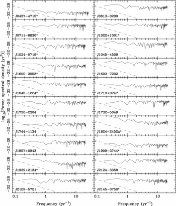
It is important to note that, for the best pulsars, e.g., PSRs J0437−4715, J1713+0747, J1857+0943, and J1909−3744, the observed power level at the lowest frequency (~0.17 yr−1) is already less than the power expected from a GW background with A
g = 10−15. However, there are some important caveats here. The GW background line is the average for an infinite number of universes. Any given realisation (e.g., our own Universe) may have a higher or lower spectrum. In setting a limit on the actual GW background, it is standard practice (e.g., Jenet et al. Reference Jenet2006) to take a value for which 95% of the realisations have a detection statistic that is greater than the statistic for the observed spectrum. Also, a comparison of the GW prediction with the measured spectra assumes that the Cholesky method compensates for the effects of fitting for ν and
$\dot{\nu }$
on the post-fit residuals and their spectrum. The accuracy of this compensation depends on the accuracy of the estimation of the red-noise spectral model and this is difficult when the red noise and white noise are of comparable amplitude. Despite these caveats, we can safely conclude that the low-frequency noise level seen in our best pulsars is already close to the average level expected for an A
g = 10−15 stochastic background.
Conversely, it is clear that the red noise in the ‘worst’ of our pulsars cannot result from the GW background. If these signals were from a GW background, they should be present in the timing residuals of all pulsars and they are not. In fact, these red signals cannot result from any ‘global’ process such as timescale or solar-system ephemeris errors which affect all pulsars. This is true even if there are geometric factors that depend on the pulsar and/or source position, since it is very unlikely that our best pulsars would all happen to be located near the nulls of the geometric pattern. The most likely sources of pulsar-specific red noise are intrinsic timing irregularities and uncorrected interstellar variations.
These results lead to a key question for PTA projects: to what extent will achievement of PTA goals be affected by intrinsic low-frequency pulsar period noise as data spans increase? Intrinsic fluctuations are of course uncorrelated between different pulsars and so, with a big enough pulsar sample, they will not preclude the reaching of PTA objectives which inherently depend on the detection of correlated signals. However, there is no doubt that they make the task much more difficult, especially if the intrinsic noise is of greater amplitude than the target signal.
The degree to which extension of data spans helps GW detection efforts depends critically on the spectral slope of the intrinsic red noise. As Table 8 and Figure 11 show, about half of the PPTA pulsars have detectable red timing noise. An estimation of the spectral properties of the red noise is difficult as, with a couple of notable exceptions, viz., PSRs J1824−2452A and J1939+2134, the red signal is only marginally above the white-noise level even at the lowest observed frequencies. Nevertheless, in order to make a first estimate of the spectral properties, we fitted a power law plus a constant (white) spectral model to the spectra shown in Figure 11. Only four pulsars (J1024−0719, J1643−1224, J1824−2452A, and J1939+2134) had power-law spectral indices greater than 2.5 and for only one of these (J1024−0719) was the spectral index comparable with that of the expected GW spectrum. We emphasise that these estimates have considerable uncertainty, but it is clear that, for the majority of the PPTA MSPs, any red timing noise detected so far has a spectrum that is much flatter than the expected GW spectrum. We cannot preclude the presence of a currently invisible red (non-GW) signal with a steep spectrum. However, with that proviso and given current models for the origin of the GW background, we can assert that within the next decade a GW signal should be dominating the residuals of several of our pulsars and hence that a significant detection of that GW signal can be expected.
4.6 The Extended PPTA Data Sets
The most important of the PTA objectives described in Section 1 are for detection of phenomena that generate low-frequency fluctuations in residual time series, i.e., the spectra of the expected signals are very red. Consequently, it is highly advantageous to utilise data sets with long spans when searching for these phenomena; this is discussed more quantitatively in Section 5 for the case of GW detection. The PPTA data sets for the 20 observed pulsars have data spans of approximately six years. However Parkes timing data were obtained for most of these pulsars for up to 11 years prior to the start of the PPTA project (Verbiest et al. Reference Verbiest2008, Reference Verbiest2009). In Appendix A, we present a reanalysis of these data sets that enables them to be smoothly joined to the best single-band PPTA data sets, giving data spans of up to 17.1 years.
5 FUTURE PROSPECTS
Figure 11 shows that the spectral index for the expected stochastic GW background is generally steeper than the spectral index of other red processes that currently affect pulsar timing residuals. Furthermore, most of these red processes are different for different pulsars, whereas the variations due to the GW background (and time-standard and ephemeris errors) are correlated. We can therefore be confident that, given sufficiently long data spans and a large enough sample of pulsars, PTA observations will reveal a GW background unless current predictions of its strength at nanohertz frequencies are incorrect.
Figure 12 shows the dependence of PTA sensitivity on the amplitude A g (Equation 1) of a stochastic GW background as a function of total data span T obs and number of pulsars in the PTA, N psr. These curves were obtained using Equation (A12) of Verbiest et al. (Reference Verbiest2009)Footnote 16 simulating an ideal PTA with N psr pulsars distributed randomly on the sky, assuming weekly ToA sampling, 100-ns rms uncorrelated timing residuals, and no ‘red’ noise contributions from sources other than the GW signal.
Sensitivity of a PTA to a stochastic background of GWs as a function of total data span T obs, number of pulsars N in the PTA, and assuming 100-ns rms timing residuals. Black lines are for N psr = 20 and T obs of 5 yr (unmarked), 10 yr (×), and 20 yr (○), respectively, red lines are similar for N psr = 50 and blue lines for N psr = 200.

The lowest black line is the PPTA ‘reference’ case discussed by Jenet et al. (Reference Jenet, Hobbs, Lee and Manchester2005). Doubling the observing time decreases the GW amplitude required for detection at a given significance level by a factor of approximately 4.5 ~ 213/6 (cf., Equation (3), remembering that the significance is in terms of amplitude rather than power). The effect of doubling observing time on significance at a given amplitude greatly depends on the level of the GW amplitude; generally, it is smaller for larger amplitudes because the GWs passing over the pulsars contribute an uncorrelated noise term, thereby reducing the significance. Increasing the number of pulsars in the PTA improves the significance at a given GW amplitude by approximately [N psr(N psr−1)]1/2 ~ N psr. Increasing the white-noise rms amplitude by a factor of five, to 500 ns, has almost exactly the same effect as halving the data span, i.e., 10 years with rms residual of 500 ns gives essentially the same sensitivity curve as five years with 100-ns rms residual. Given the sensitivity, we can achieve with current instruments, the 10-year–500-ns scenario is more realistic for the PPTA to achieve the necessary detection sensitivity.
Improving rms timing residuals will also help, but this is difficult with present telescope facilities. In the Northern Hemisphere, there are a number of radio telescopes with collecting area larger than that of the Parkes telescope which should give better results given similar instrumentation and similar observing cadence. For Parkes, a more sensitive broadband receiver is currently under development and this will give improved results.
However, as Figure 12 makes it clear, the greatest benefit is obtained by increasing the number of pulsars in the PTA. Ongoing searches (e.g., Keith et al. Reference Keith2012a) have already found MSPs which are suitable for PTAs and the best of these have already been included in existing PTAs. In time, these will contribute fully to PTA sensitivity. This approximately linear increase in PTA sensitivity with N psr is the strongest motivation to combine the results from the three existing (and possible future) PTA projects. The EPTA, NANOGrav, and the PPTA are collaborating to form the International Pulsar Timing Array (IPTA) (Hobbs et al. Reference Hobbs2010b). Although there is considerable overlap between the samples of the three main existing PTA projects, Hobbs et al. (Reference Hobbs2010b) list 37 pulsars that are regularly observed by at least one PTA. Of course, the data quality varies considerably across this sample, but there is no doubt that an IPTA data set will give superior results compared with the data set of any one participating PTA. Even at the pessimistic end of current predictions (e.g., Sesana et al. Reference Sesana, Vecchio and Colacino2008), IPTA data sets with spans of 10 years or more should give a significant detection of the GW background from binary black holes in distant galaxies. Failure to detect the GW background with these data sets will imply that current models for this background are fundamentally flawed. This would have important implications for current theories of black hole formation and evolution in galaxies and for theories of galaxy growth through mergers.
Even if a detection of GWs is achieved with IPTA data sets, it is clear that detailed study of the properties of nanohertz GWs and their sources will have to wait until the SKA (see, e.g., Cordes et al. Reference Cordes, Kramer, Lazio, Stappers, Backer and Johnston2004) is operational. The enormous increase in sensitivity provided by the SKA will allow detection and subsequent frequent timing observations of a large sample of MSPs. Ultimately, a sample of 200 PTA-quality MSPs should be possible, although it will take time to build up a significant data span. Once that is done, Figure 12 shows that high-significance detections will be possible even if the GW background is relatively weak, enabling accurate measurement of properties such as spectral index and possible origin of the background (e.g., van Haasteren et al. Reference van Haasteren2011) and investigation of non-GR effects in the received signals (e.g., Lee et al. Reference Lee, Jenet and Price2008).
Although Figure 12 is computed for the case of detection of a stochastic GW background, similar considerations apply to other PTA objectives. Improved data sets should enable the detection and study of individual GW sources, for example, bright black hole binaries (Sesana et al. Reference Sesana, Vecchio and Volonteri2009) or burst signals from cosmic strings (Damour & Vilenkin Reference Damour and Vilenkin2005; Sanidas et al. Reference Sanidas, Battye and Stappers2012). Source locations with arcminute precision or better should be measurable and other source properties can be studied in detail (Lee et al. Reference Lee, Wex, Kramer, Stappers, Bassa, Janssen, Karuppusamy and Smits2011). Extended data sets give improved pulsar-based timescales (Hobbs et al. Reference Hobbs2012), enable improved determinations of the masses of solar-system planets, and possibly even allow the detection of currently unknown solar-system objects such as TNOs. The future prospects of PTA research are indeed exciting.
ACKNOWLEDGMENTS
The PPTA project was initiated with support from RNM’s Australian Research Council (ARC) Federation Fellowship (FF0348478) and from the CSIRO under this Fellowship program. It has also received support from ARC Discovery Project grant DP0985272. GH is the recipient of an ARC QEII Fellowship (DP0878388) and VR is a recipient of a John Stocker Postgraduate Scholarship from the Science and Industry Endowment Fund. Part of this research was carried out at the Jet Propulsion Laboratory, California Institute of Technology, under a contract with the National Aeronautics and Space Administration. We acknowledge contributions to the project from L. Kedziora-Chudczer, K. J. Lee, A. N. Lommen, D. Smith, and Ding Chen. The Parkes telescope is part of the Australia Telescope which is funded by the Commonwealth Government for operation as a National Facility managed by CSIRO.
APPENDIX A. EXTENSION OF THE PPTA DATA SETS
Many of the PPTA pulsars had been observed at Parkes for some years prior to the commencement of the PPTA project (e.g., Toscano et al. Reference Toscano, Sandhu, Bailes, Manchester, Britton, Kulkarni, Anderson and Stappers1999; Hotan et al. Reference Hotan, Bailes and Ord2006). Long data spans are very beneficial to many pulsar timing studies and so it is useful to combine these earlier data with the PPTA observations. Here, we describe the ‘extended PPTA’ data sets that add earlier observations as described by Verbiest et al. (Reference Verbiest2008, Reference Verbiest2009) to the PPTA data sets.
Verbiest et al. (Reference Verbiest2008) analysed Parkes observations of PSR J0437−4715 obtained over a 10-year period from 1996 to 2006 using two different receivers (H-OH and multibeam centre beam) operating in the 20-cm band and with four different backend systems operating at different times. With these data, they obtained a precise distance for the pulsar, both with a direct measurement of the annual parallax and by measuring the apparent orbital period derivative resulting from the transverse motion of the system. The backend systems used were the fast pulsar timing machine (FPTM) (Sandhu et al. Reference Sandhu, Bailes, Manchester, Navarro, Kulkarni and Anderson1997) in 1996–1997, the S2 VLBI recorder (van Straten Reference van Straten2003) in 1997–1998, the Caltech–Parkes–Swinburne recorder CPSR (van Straten Reference van Straten2003) for 1998–2002, and CPSR2 for 2002–2006.
Similarly, Verbiest et al. (Reference Verbiest2009) presented 20-cm data for all 20 PPTA pulsars with data spans ranging from 3.9 years to 14.2 years recorded between 1994 and 2008. The FPTM was used from 1992 to 2001, a 512-channel analogue filterbank (D’Amico et al. Reference D’Amico, Lyne, Manchester, Possenti and Camilo2001) in 2002 and 2003 and CPSR2 from 2002 November to 2008. For three pulsars, PSRs J1045−4509, J1909−3744, and J1939+2134, data from the 50-cm receiver was used to model the DM variations after this receiver became available in 2003 November.
These data were analysed by Verbiest et al. (Reference Verbiest2008, Reference Verbiest2009) using Tempo2 and fitting for the pulsar astrometric, pulse frequency, and binary parameters (if appropriate) simultaneously with arbitrary offsets between the different instruments. As Yardley et al. (Reference Yardley2011) have shown, fitting for offsets (or jumps) subtracted most of the low-frequency power from the post-fit residuals. We have therefore reanalysed the Verbiest et al. (Reference Verbiest2008, Reference Verbiest2009) data sets to separately determine and fix as many of the offsets as possible. Where overlapping or near-overlapping (gap ≲ 150 d) data from two different instruments were available, the offsets were measured from short data spans (typically a few months) fitting for just ν and the offset with all other parameters held at the values from a fit to the entire data span for that pulsar. Offsets determined in this way were held fixed in subsequent analyses. For a few pulsars, data gaps between some pairs of instruments were too large for this procedure to give reliable results and arbitrary jumps were retained.
The Verbiest et al. (Reference Verbiest2008, Reference Verbiest2009) data sets were then combined with the three-band PPTA data sets described in the main text to form extended PPTA data sets with data spans of up to 17.1 years. These extended data sets were then analysed using Tempo2 with the Cholesky decomposition (Coles et al. Reference Coles, Hobbs, Champion, Manchester and Verbiest2011) to properly handle the red-noise component. The DM and DM offsets determined as described in Section 4.3 for the PPTA data spans were included and held fixed. Since most of the Verbiest et al. (Reference Verbiest2008, Reference Verbiest2009) observations were at frequencies in or close to the 20-cm band, it was generally impossible to obtain DM variations from these data that were sufficiently precise to enable correction for variable dispersion delays. The exception is PSR J1939+2134, where dual-band FPTM observations (band centres about 1,420 and 1,650 MHz) enabled a DM offset at MJD 50350 (1996 September) to be measured. This was held fixed in the subsequent Cholesky fit along with the other DM offsets.
For all pulsars, parameters for which significant values could be obtained were included in the fit. Finally, the remaining instrumental offsets were included. The use of the Cholesky method ensures that these offsets (along with the other parameters) and their uncertainties are reliably determined despite the presence of the red noise. The first seven columns of Table 9 give the data spans in MJD and years, the total number of ToAs (all bands), number of pulsar parameters fitted (N p), the number of fixed instrumental offsets or jumps (N j0), and the number of instrumental offsets included in the final fit (N j1). The fixed instrumental jumps include three interband jumps; the ‘best’ band is designated as reference and the other three bands (including both 40 and 50 cm) are referred to it. Fitted jumps were needed for only seven pulsars and for all of these except PSR J0437−4715, the number required was three or fewer. PSR J0437−4715 required more offsets because more instruments were used for observations of this pulsar and the high precision of the ToAs revealed a larger number of significant offsets.
The extended PPTA data sets.

To form a ‘best’ extended data set, the Verbiest et al. (Reference Verbiest2008, Reference Verbiest2009) data sets were combined with the best PPTA data set described in Section 4.4 and Table 7. Parameter files were created by copying the pulsar parameters and jumps and DM corrections for the extended three-band fit described above and holding all parameters except ν and
$\dot{\nu }$
fixed. Columns 8–10 of Table 9 give the number of ToAs in the best single-band extended data set, and the post-fit rms timing residual and reduced χ2 for each pulsar. Note that Cholesky decomposition was not used in this fit. Figure 13 shows the post-fit residuals, clearly illustrating the better quality of the PPTA data sets compared with those obtained with the earlier systems. For several pulsars, e.g., PSRs J0437−4715 and J1024−0719, they also reveal red noise that was obvious in neither the six-year PPTA data sets (Figure 10) nor in the post-fit residuals presented by Verbiest et al. (Reference Verbiest2008, Reference Verbiest2009).
Post-fit timing residuals for the extended PPTA data sets. The vertical extent of each subplot is adjusted to fit the data and its value is given below the pulsar name. The dashed line marks zero residual.

To quantify these in the same way as for the PPTA data sets (Table 8),
$\ddot{\nu }$
was additionally fitted, giving the values in the last column of Table 9. In contrast to the PPTA data sets, where 10 of the 20 pulsars had
$\ddot{\nu }$
values significant at the 3σ level, all but three of the pulsars have significant
$\ddot{\nu }$
values for the extended data set. This is a simple illustration of the importance of long data spans for characterising red-noise processes. PSR J1024−0719 is a particularly striking example: for the PPTA data set, this had a
$\ddot{\nu }$
with a significance of 5σ, whereas for the extended data set the value is consistent but the significance has increased to 48σ. It is interesting to note that, based on the PPTA data set (Section 4.5), this pulsar appears to have a relatively steep red timing noise spectrum.
PSRs J1824−2452A and J1939+2134 stand out with positive and relatively large
$\ddot{\nu }$
values, but it is notable that 13 of the 17 significant
$\ddot{\nu }$
in Table 8 are also positive. A small glitch was observed for PSRs J1824−2452A in 2001 (Cognard & Backer Reference Cognard and Backer2004). It is well known that large positive values of
$\ddot{\nu }$
are observed after glitches in young pulsars (Lyne et al. Reference Lyne, Shemar and Graham-Smith2000; Yuan et al. Reference Yuan, Wang, Manchester and Liu2010). These are attributed to the dynamics of superfluid vortices in the interior of the neutron star as they re-establish equilibrium with the rigid crust following a glitch (e.g., Alpar et al. Reference Alpar, Chau, Cheng and Pines1993). This suggests the intriguing possibility that the observed positive
$\ddot{\nu }$
values are attributable to post-glitch recoveries, in all cases, except possibly for PSR J1824−2452A, from unseen earlier glitches. It is worth noting that the
$\ddot{\nu }$
values seen for the PPTA MSPs are about four orders of magnitude smaller than those seen in young pulsars.
Comparison of the observed rms timing residuals for the extended data sets with the ‘CP+MSP’ model of Shannon & Cordes (Reference Shannon and Cordes2010) gives similar results with those for the PPTA data sets discussed in Section 4.5. Compared with the PPTA data sets, the ζ values for most pulsars are a factor of 2–8 smaller, indicating the diminished relative contribution of the white noise with the longer data spans. For PSR J0437−4715, ζ ~ 0.15 showing that the model substantially overpredicts the amount of timing noise with this longer data span. For PSRs J1909−3744 and J1939+2134, ζ values are 1.18 and 0.49, respectively, similar to those for the shorter data spans; for PSR J1824−2452A there are no new data in the extended data set.
For several pulsars, most notably PSRs J0437−4715 and J1713+0713, there is significant red noise in the Verbiest et al. (Reference Verbiest2008, Reference Verbiest2009) data sets alone, which was not present in the results presented by Verbiest et al. (Reference Verbiest2008, Reference Verbiest2009). This is mostly attributable to the fixing of the instrumental offsets. However, it is likely that the inability to accurately model DM variations for most of the early data also contributes significantly to the observed residuals. For example, the deviations observed in the early data for PSR J1045−4509 are almost certainly due to uncorrected DM variations (cf., Keith et al. Reference Keith2012b). It is possible that observations from other observatories will help to determine pre-PPTA DM variations. However, it is generally difficult if not impossible to establish absolute ToAs for archival data with sufficient precision and so these data are likely to be of limited use in this respect. Only future carefully calibrated multiband observations will establish for sure if DM variations are a significant contributor to the observed red noise on decade-long timescales.


